MEASURING SPATIAL EFFECTS IN PARAMETRIC AND NONPARAMETRIC MODELLING OF REGIONAL GROWTH AND CONVERGENCE Giuseppe Arbia, Roberto Basile and Mirella Salvatore ____________________________________ Paper prepared for the UNU/WIDER Project Meeting on Spatial Inequality in Development Helsinki, 29 May 2003
Transcript
MEASURING SPATIAL EFFECTS IN PARAMETRIC AND
NONPARAMETRIC MODELLING OF REGIONAL GROWTH AND CONVERGENCE
Giuseppe Arbia, Roberto Basile and Mirella Salvatore
____________________________________ Paper prepared for the UNU/WIDER Project Meeting on
Spatial Inequality in Development Helsinki, 29 May 2003
2
Measuring Spatial Effects in Parametric and
Nonparametric Modelling of Regional Growth and
Convergence
by
Giuseppe Arbia*, Roberto Basile** and Mirella Salvatore*
ABSTRACT
Testing regional convergence hypothesis involves important data issues. In empirical circumstances the problem arises of finding the best data to test the theory and the best estimators for the associated modelling. In the literature usually little attention is given to the level of spatial aggregation used and to the treatment of the spatial dependence and spatial heterogeneity. In this paper, we present an empirical study of per capita income convergence in Italy based on a fine level of aggregation (the NUTS-3 EU regions represented by the 92 Italian provinces). Concerning the statistical methodology, we compare two different approaches to measure the effects of spatial heterogeneity and spatial dependence. Our results confirm the convergence club hypothesis and suggest that spillover and convergence clubs are spatially concentrated.
Keywords: Nonparametric analysis; Regional convergence; Regional spill-over; Stochastic kernels; Spatial dependence modelling; Spatial regimes. JEL: C13, O00, R11 * Department of Sciences, Faculty of Economics, University “G. D’Annunzio”, Viale Pindaro, 42, 65127 Pescara (Italy), [email protected]; [email protected]. **ISAE (Institute for Studies and Economic Analyses), P.zza Indipendenza, 4, 00191 Rome. Tel. +39-06-44482874, E-mail: [email protected].
3
1. Introduction
One of the most striking features of empirical economic data is that some
countries and regions within a country grow faster than others. Economic theory has
long been aware of this problem and various explanations have been provided in the
past (Solow, 1956; and Barro & Sala-i-Martin, 1995 for a review). A certain school of
thought reached an optimistic view of reality by predicting that a set of economies
(countries or regions) will tend to assume a common level of output per capita (that is
they will “converge”) in the presence of constant returns to scale and decreasing
productivity of capital. However, many empirical studies show contrasting, less
optimistic, results.
Apart from the evident interest in the subject at a World scale, regional
convergence studies have recently experienced an acceleration of interest due to the
issues raised in Europe by the unification process. Since large differentials in per capita
GDP across regions are regarded as an impediment to the completion of the economic
and monetary union, the narrowing of regional disparities is indeed regarded as a
fundamental objective for the European Union policy. Hence, the problem of testing
convergence among the member States of the Union and measuring its speed emerges
as a fundamental one in the view of policy evaluation.
Surprisingly enough, the literature on the empirical measurement of spatial
convergence has not moved at the same speed with the increased demand. Indeed, most
of the empirical work is still based on the computation of some basic statistical
measures in which the geographical characteristics of data play no role. For instance, in
their celebrated paper Barro and Sala-i-Martin (1992) base their models on parameters
like the variance of logarithm (to identify a σ-convergence) and the simple regression
coefficients (to identify a β-convergence) estimated using standard OLS procedures. In
general most empirical studies in this field base their conclusions on cross-sectional data
referred to geographical units almost systematically neglecting two remarkable features
of spatial data. First of all, spatial data represent aggregation of individuals within
arbitrary geographical borders that reflect political and historical situations. The choice
of the spatial aggregation level is therefore crucial because different partitions can lead
to different results in the modelling estimation phase (Arbia, 1988). Secondly, it is well
known that regional data cannot be regarded as independently generated because of the
4
presence of spatial similarities among neighbouring regions (Anselin, 1988; Anselin and
Bera, 1998). As a consequence, the standard estimation procedures employed in many
empirical studies can be invalid and lead to serious biases and inefficiencies in the
estimates of the convergence rate.
In this paper, we present an empirical study of the long-run convergence of per
capita income in Italy (1951-2000) based on a level of aggregation (the NUTS 3 EU
regions corresponding to the 92 Italian provinces) which is fine enough to allow for
spatial effects (like spatial regimes and regional spill-overs) to be properly modelled.
The empirical analysis is divided into parts. In the first one, we use “traditional”
techniques, i.e. σ- and β−convergence approaches. As far as the β−convergence analysis
is concerned, a non-parametric local regression model is firstly applied to identify non-
linearities (i.e. multiple regimes) in the relationship between growth rates and initial
conditions. Then, by using information on the presence of spatial regimes, we apply
cross section regressions accounting for spatial dependence. In the second empirical
part, we exploit the alternative kernel density approach (based on the concept of intra-
distribution dynamics) suggested by Quah (1997) and we investigate the role of spatial
dependence by applying a proper conditioning scheme.
The layout of the paper is the following. In Section 2, we present a review of spatial
econometric techniques that incorporate spatial dependence and spatial heterogeneity
within the contest of a β-convergence modelling. In Section 3, we report the results of
an empirical analysis based on the 92 Italian provinces (European NUTS-3 level) and
the per capita income recorded in the period ranging from 1951 to 2000 and we show
the different estimates of the convergence speed obtained by using different modelling
specifications for spatial effects. In Section 4, we discuss some possibility of including
spatial dependence in stochastic kernels estimation and provide empirical evidences
based on the same data set. Finally, in Section 5 we discuss the results obtained and
outline possible extensions of the present work.
2. Spatial dependence and spatial regimes in cross-section growth
behaviour
The most popular approaches in the quantitative measurement of convergence are
those based on the concepts of σ- and β-convergence (Durlauf and Quah, 1999 for a
5
review). Alternative methods are the intra-distribution dynamics approach (Quah, 1997;
Rey, 2000) and, more recently, the Lotka-Volterra predator-prey specification (Arbia
and Paelinck, 2002).
2.1 σ-convergence
The σ-convergence approach consists on computing the standard deviation of
regional per capita incomes and on analysing its long-term trend. If there is a decreasing
trend, then regions appear to converge to a common income level. Such an approach
suffers from the fact that the standard deviation is a measure insensible to spatial
permutations and, thus, it does not allow to discriminate between very different
geographical situations (Arbia, 2001).1 Furthermore, as argued by Rey and Montoury
(1998), σ-convergence analysis may “mask nontrivial geographical patterns that may
also fluctuate over time” (p. 7-8). Therefore, it is useful to analyse the geographical
dimensions of income distribution in addition to the dynamic behaviour of income
dispersion. This can be done, for instance, by looking at the pattern of spatial
autocorrelation based on the Moran’s I statistics (Cliff and Ord, 1973).
2.2 β-convergence
So far, the β-convergence approach has been considered as one of the most
convincing under the economic theory point of view. It also appears very appealing
under the policy making point of view, since it quantifies the important concept of the
speed of convergence. It moves from the neoclassical Solow-Swan exogenous growth
model (Solow, 1956; Swan, 1956), assuming exogenous saving rates and a production
function based on decreasing productivity of capital and constant returns to scale. On
this basis authors like Mankiw et al. (1992) and Barro and Sala-i-Martin (1992)
suggested the following statistical model
1 Consider two regions each dominating the extreme end of an income scale. Now let there be mobility along the income scale. For the sake of argument, say each ended up at the exact position formerly occupied by its counterpart. According to the concept of σ convergence, nothing has changed. In reality the poor has caught up with the rich while the rich has slide down to the position of the poor.
6
ititit
ikt
y
y,,
,
,ln εµ +=
+ (1)
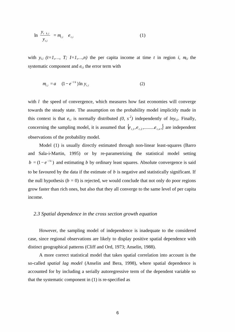
with yt,i (t=1,…, T; I=1,…,n) the per capita income at time t in region i, µt,i the
systematic component and εt,i the error term with
itk
it ye ,, ln)1( λαµ −−+= (2)
with λ the speed of convergence, which measures how fast economies will converge
towards the steady state. The assumption on the probability model implicitly made in
this context is that εt,i is normally distributed (0, σ2) independently of lnyt,i. Finally,
concerning the sampling model, it is assumed that { },,........., ,2,1, nttt εεε are independent
observations of the probability model.
Model (1) is usually directly estimated through non-linear least-squares (Barro
and Sala-i-Martin, 1995) or by re-parametrizing the statistical model setting
)1( ke λβ −−= and estimating β by ordinary least squares. Absolute convergence is said
to be favoured by the data if the estimate of β is negative and statistically significant. If
the null hypothesis (β = 0) is rejected, we would conclude that not only do poor regions
grow faster than rich ones, but also that they all converge to the same level of per capita
income.
2.3 Spatial dependence in the cross section growth equation
However, the sampling model of independence is inadequate to the considered
case, since regional observations are likely to display positive spatial dependence with
distinct geographical patterns (Cliff and Ord, 1973; Anselin, 1988).
A more correct statistical model that takes spatial correlation into account is the
so-called spatial lag model (Anselin and Bera, 1998), where spatial dependence is
accounted for by including a serially autoregressive term of the dependent variable so
that the systematic component in (1) is re-specified as
7
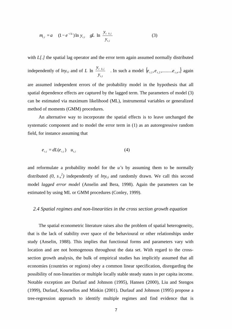
+−+= +−
it
iktit
kit y
yLye
,
,,, lnln)1( γαµ λ (3)
with L[.] the spatial lag operator and the error term again assumed normally distributed
independently of lnyt,i and of
+
it
ikt
y
yL
,
,ln . In such a model { },,........., ,2,1, nttt εεε again
are assumed independent errors of the probability model in the hypothesis that all
spatial dependence effects are captured by the lagged term. The parameters of model (3)
can be estimated via maximum likelihood (ML), instrumental variables or generalized
method of moments (GMM) procedures.
An alternative way to incorporate the spatial effects is to leave unchanged the
systematic component and to model the error term in (1) as an autoregressive random
field, for instance assuming that
ititit uL ,,, )( += εδε (4)
and reformulate a probability model for the u’s by assuming them to be normally
distributed (0, σu2) independently of lnyt,i and randomly drawn. We call this second
model lagged error model (Anselin and Bera, 1998). Again the parameters can be
estimated by using ML or GMM procedures (Conley, 1999).
2.4 Spatial regimes and non-linearities in the cross section growth equation
The spatial econometric literature raises also the problem of spatial heterogeneity,
that is the lack of stability over space of the behavioural or other relationships under
study (Anselin, 1988). This implies that functional forms and parameters vary with
location and are not homogenous throughout the data set. With regard to the cross-
section growth analysis, the bulk of empirical studies has implicitly assumed that all
economies (countries or regions) obey a common linear specification, disregarding the
possibility of non-linearities or multiple locally stable steady states in per capita income.
Notable exception are Durlauf and Johnson (1995), Hansen (2000), Liu and Stengos
(1999), Durlauf, Kourtellos and Minkin (2001). Durlauf and Johnson (1995) propose a
tree-regression approach to identify multiple regimes and find evidence that is
8
consistent with a multiple-regime data-generating process as opposed to the traditional
one-regime model. Hansen (2000) uses a Threshold Regression model to formally test
for the presence of a regime shift. Liu and Stengos (1999) employ a semi-parametric
approach to model the regression function and, as in Durlauf and Johnson and Hansen,
emphasize the role of initial output and schooling as variables with a potential to affect
growth in a non linear way through possible thresholds or otherwise. Durlauf,
Kourtellos and Minkin (2001)use a local polynomial growth regression to explicitly
allow for cross-country parameter heterogeneity.
The basic idea underlying the multiple regime analysis is that the level of per
capita GDP on which each economy converges depends on some initial conditions
(such as initial per capita GDP or initial level of schooling), so that, for example,
regions with an initial per capita GDP lower than a certain threshold level converge to
one steady state level while regions above the threshold converge to a different level. A
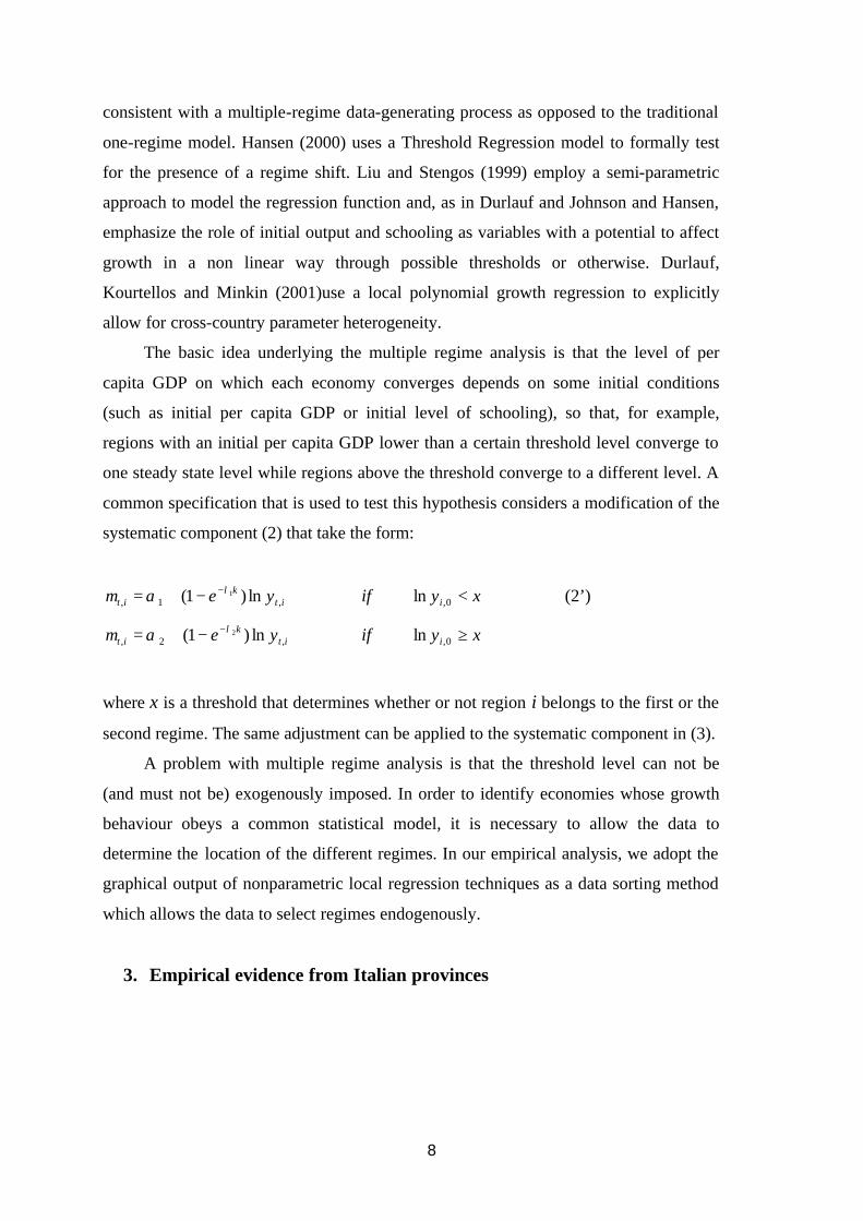
common specification that is used to test this hypothesis considers a modification of the
systematic component (2) that take the form:
itk
it ye ,1, ln)1( 1λαµ −−+= if xyi <0,ln (2’)
itk
it ye ,2, ln)1( 2λαµ −−+= if xyi ≥0,ln
where x is a threshold that determines whether or not region i belongs to the first or the
second regime. The same adjustment can be applied to the systematic component in (3).
A problem with multiple regime analysis is that the threshold level can not be
(and must not be) exogenously imposed. In order to identify economies whose growth
behaviour obeys a common statistical model, it is necessary to allow the data to
determine the location of the different regimes. In our empirical analysis, we adopt the
graphical output of nonparametric local regression techniques as a data sorting method
which allows the data to select regimes endogenously.
3. Empirical evidence from Italian provinces
9
The empirical study focuses on the case of Italian provinces, which correspond to
the European NUTS-3 level in the official UE classification.2 The analysis is based on a
newly compiled database on per capita GDP for the 92 provinces over the period 1951-
2000.3
We start with a σ-convergence analysis of per capita income in the 92 provinces
and the related spatial patterns over the period 1951-2000 (Section 3.1). In Section 3.2,
3.3 and 3.4 we will move to the β-convergence analysis by taking explicitly into
consideration the spatial heterogeneity and the spatial dependence patterns displayed by
data.
3.1 σ convergence and spatial autocorrelation
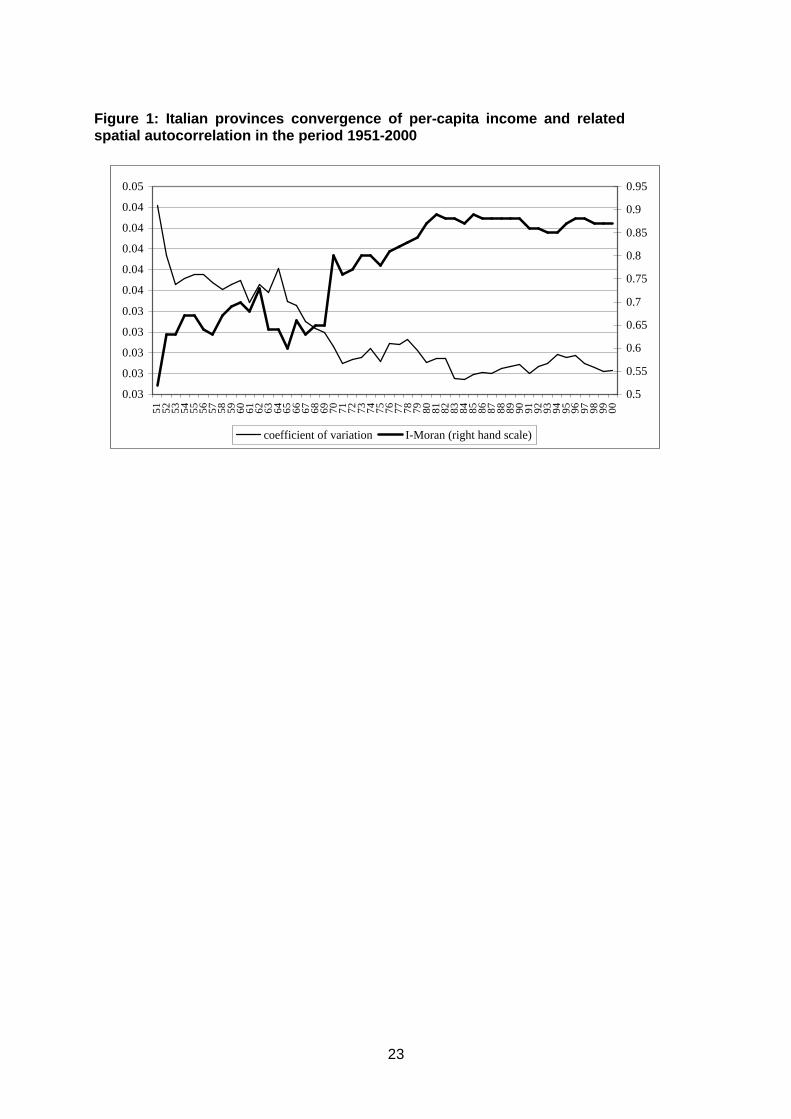
Figure 1 shows the dynamics of the provinces’ real per capita GDP dispersion,
measured in log terms, over the period 1951-2000, synthetically measured by its
coefficient of variation (the ratio between the standard deviation and the national
average). Regional inequalities diminished by more than one half over the entire period,
but the sharp trend towards convergence was confined to the period between 1951 and
1970. This is due partly to the significant effort to ‘exogenously’ implement economic
development in the South (through the Cassa del Mezzogiorno) and partly to the
‘endogenous’ development of the North-Eastern regions (through the emergence of
industrial districts). The following period was, instead, characterized by a substantial
invariance of the income inequalities.
Figure 1 also displays the pattern of spatial autocorrelation for the provincial
incomes over the same period of time, based on the Moran’s I statistics. There is very
strong evidence of spatial dependence as the I-Moran statistics are significant (at the
probability level 0.01) for each year. Differently from Rey and Montoury (1998) that
examined the case of the United States, however, convergence and spatial dependence
tend to move in the same direction (the simple correlation between Moran’s I statistics
2 The compilation of provincial data on value added has been based on estimates elaborated by the Istituto Guglielmo Tagliacarne, which involve the adoption of direct and indirect provincial indicators to disaggregate regional product within provinces. These estimates have been transformed at constant prices by using sectoral/regional value added deflators. The source of population data is ISTAT (National Institute of Statistics). 3 Italy is currently divided into 103 provinces, grouped into 20 regions. Over the period considered (1951-1999), however, the boundaries of some administrative provinces changed. Only the provinces that already existed in 1951 (92 units) have been considered for the empirical analysis.
10
and the coefficient of variation is –0.9). The minimum level of spatial dependence was
registered for the first year of the sample (1951), when the income dispersion was at its
maximum level. Then, I-Moran increased very strongly till the ‘70s, that is the period of
strong convergence. Finally, it remained stable and high over the ’90s.
Figure 1
Thus, after reaching a stable level of a-spatial inequality (measured by the
coefficient of variation) in 1970, it follows a period of strong polarization at constant
levels of inequality (for a distinction between a-spatial inequality and polarization, see
Arbia, 2000, 2001).
3.2 β convergence: basic results
We start from the OLS estimates of the unconditional model of β-convergence
and test for the presence of different possible sources of model misspecification (spatial
heteroskedasticity and spatial autocorrelation). The general objective of this analysis is
to assess whether the results of previous studies at provincial level (e.g. Fabiani and
Pellegrini, 1997; Cosci and Mattesini, 1995), carried out using the OLS method, were
actually biased for the presence of spatial effects.
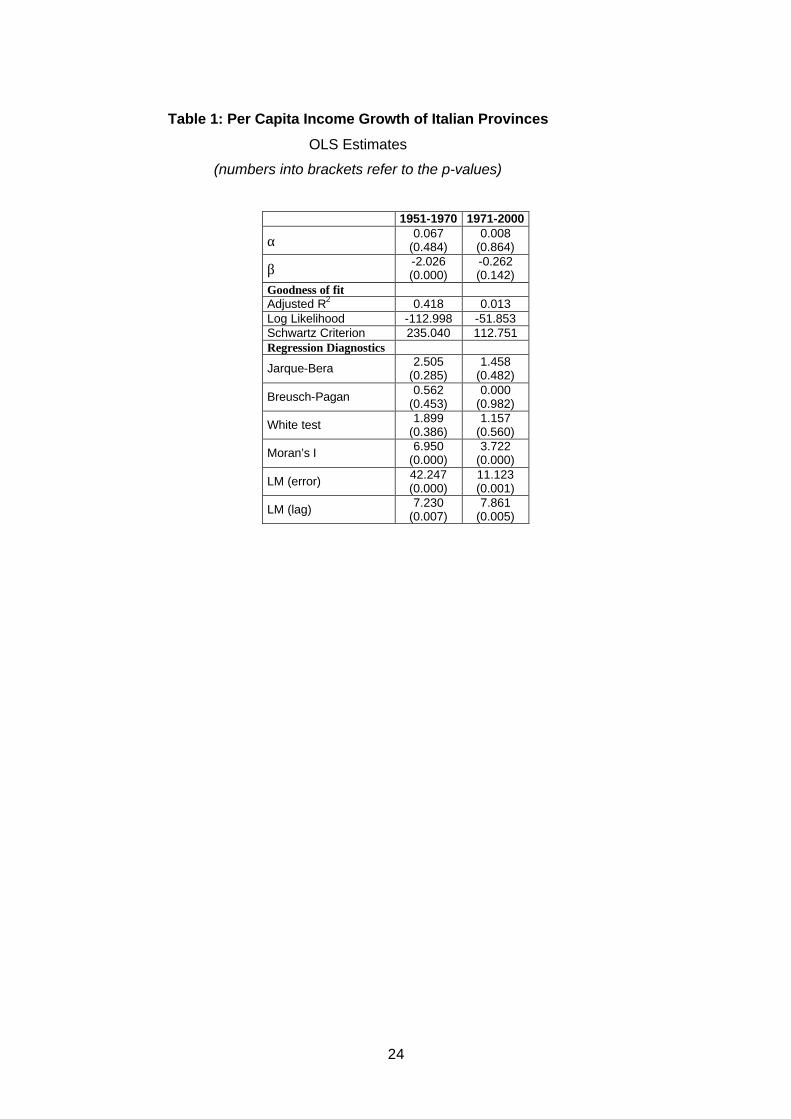
Table 1 displays the cross-sectional OLS estimates of absolute convergence for
the 92 Italian provinces. The dependent variable of the model is the growth rate of
province’s per capita income, while the predictor introduced in each model is the initial
level of per-capita income (expressed in natural logarithms). Both variables are scaled
to the national average. In order to consider the trend break identified in the σ
convergence analysis, we estimate models for the two periods 1951-1970 and 1971-
2000.
Table 1
Our results appear very much in line with the previous findings on the
development of Italian regions/provinces. The coefficient of initial per capita GDP is –
2.03 and significant at p<0.01 for the first period- confirming the presence of absolute
11
convergence over that period, while it is –0.26 and non-significant for the second period
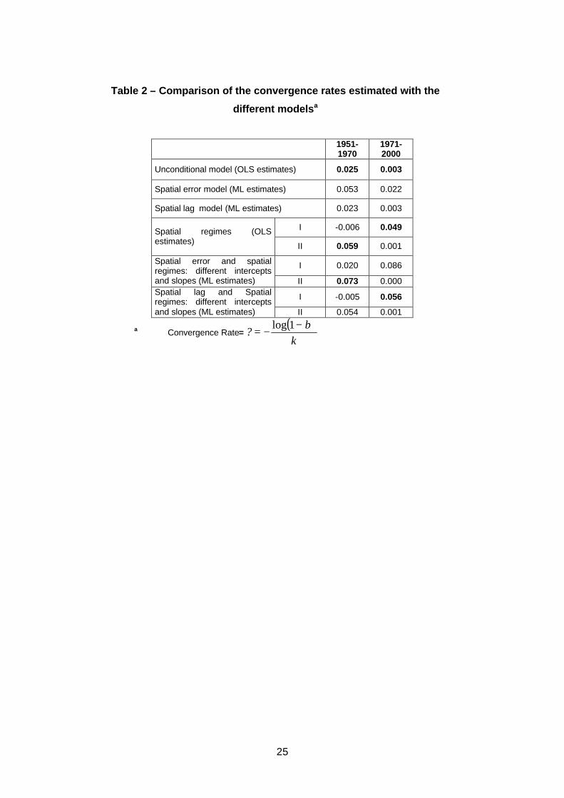
- suggesting lack of convergence.4 Similarly, the convergence rate was fairly high
(2.5%) during the first period and declined substantially (to 0.3%) during the period
1970-2000. The lack of β-convergence starting from the beginning of the '70s was also
suggested by Paci and Pigliaru (1995), Cellini and Scorcu (1995) and Fabiani and
Pellegrini (1997).
Table 2
Table 1 also reports some diagnostics to identify misspecifications in the OLS
cross-sectional model. Firstly, the Jarque-Bera normality test is always far from
significant. Consequently, we can safely interpret the results of the various
misspecification tests (heteroskedasticity and spatial dependence tests) that depend on
the normality assumption, such as the various Lagrange Multiplier tests.5 Since no
problems were revealed with respect to a lack of normality, the Breusch-Pagan statistic
is given. Its values are far from significant, indicating that there are no
heteroskedasticity problems. This is confirmed by the robust White statistics.
The last specification diagnostics refers to spatial dependence. Three different
tests for spatial dependence are included: a Moran’s I test and two Lagrange multiplier
(LM) tests. As reported in Anselin and Rey (1991), the first one is very powerful against
both forms of spatial dependence: the spatial lag and spatial error autocorrelation.
Unfortunately, it does not allow discriminating between these two forms of
misspecification. Both LM (error autocorrelation) and LM (spatial lag) have high values
and are strongly significant, indicating significant spatial dependence, with an edge
towards the spatial error.
The results described so far suggest that the original unconditional model, which
has been the workhorse of much previous research, suffers from a misspecification due
to omitted spatial dependence. Thus, we attempt alternative specifications. An
approach, adopted for the case of the United States by Rey and Montoury (1998),
4 σ and β convergence analyses thus give coherent results, suggesting that in our case Galton fallacy (Quah, 1993) does not represent a serious problem. 5 Heteroscedasticity tests have been carried out for the case of random coefficient variation (the squares of the explanatory variables were used in the specification of the error variance to test for additive heteroscedasticity).
12
consists of the application of spatial econometric tools directly to the unconditional
model.
An alternative approach, proposed in this paper, consists of firstly detect and
identifying the presence of spatial regimes, and then using maximum likelihood spatial
dependence models to control for the presence of spatial autocorrelation. This approach
is based on the assumption that the observed spatial autocorrelation might depend (at
least in part) on heterogeneity (multiple regimes), in the form of different intercepts
and/or slopes in the regression equation for subsets of the data.
3.3 Non-linearities in cross section growth behaviour
The main concern of this section is the identification of growth patterns (non-
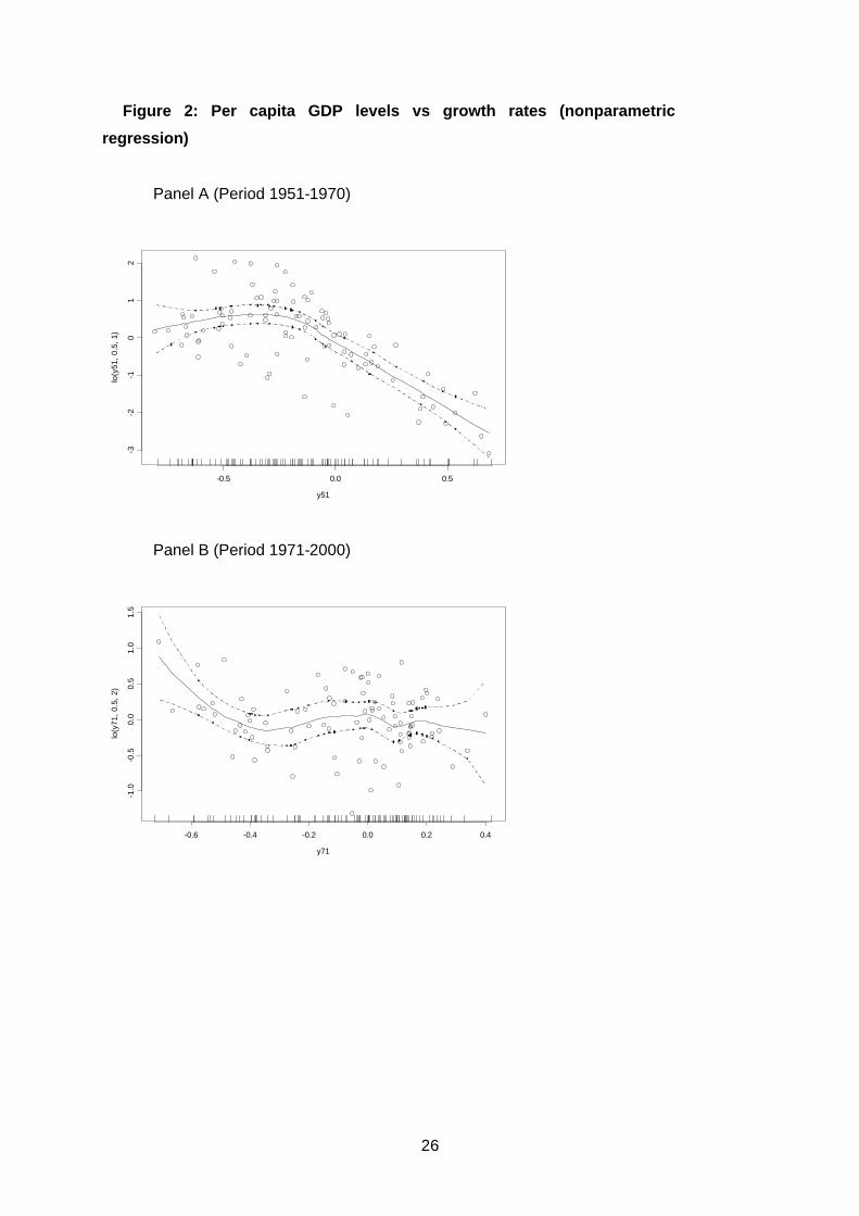
linearities) in the data. In figure 2 we plot the growth rate against initial per capita GDP
for the two periods 1951-70 and 1971-2000, and a nonparametric estimation of the
relationship between these two variables.6
The nonparametric regressions in figure 2 identify non-linear relationships between
the level of GDP and the growth rate. In particular, for the period 1951-70 (Panel A), at
low income levels (that is initial levels of relative log incomes lower than –0.26) growth
rates are high and slightly increasing (denoting a diverging process), while regions with
relative initial incomes higher than –0.26 follow a converging path. For the period
1971-2000, at low income levels growth rates are initially high and then decreasing up
to a minimum (corresponding to a relative log of GDP per capita of –0.34). After that
level, we cannot observe any relationship between the two variables. These results
suggest that the initial income coefficient in the miss-specified linear model inherits the
convergence exhibited among regions associated with a common steady state in the
correctly specified multiple regime process.
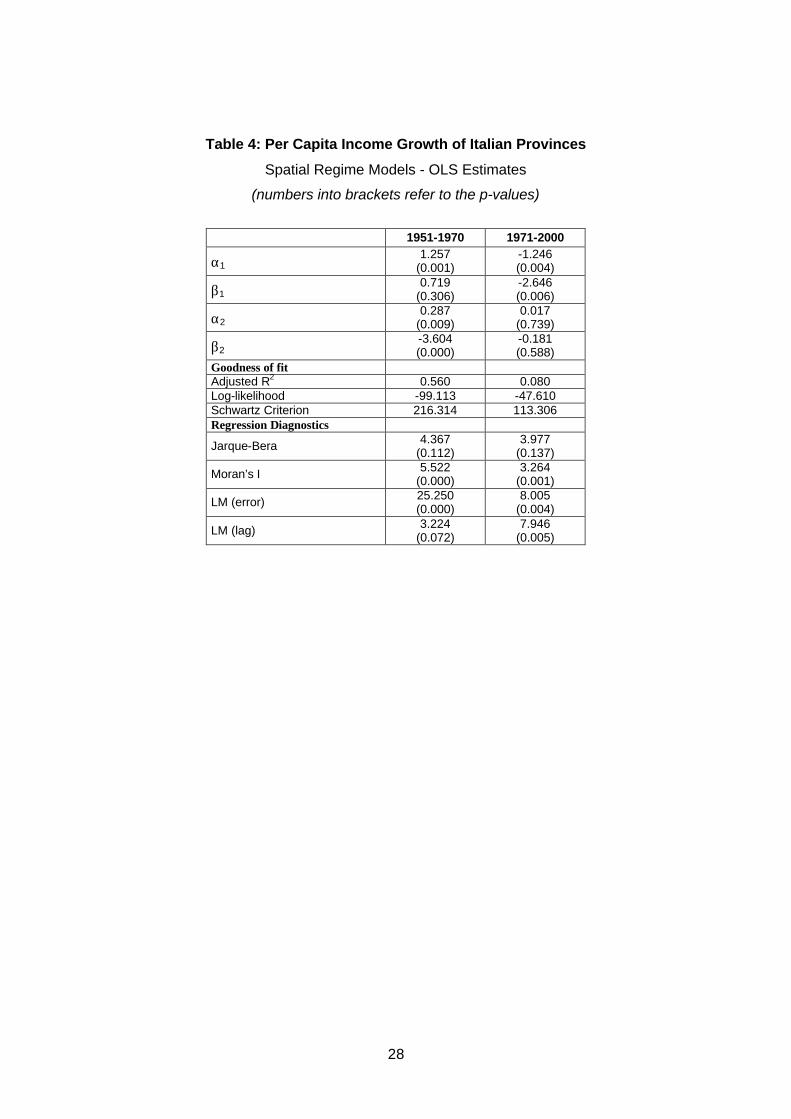
By using this information, we split the sample in two regimes for both periods (see
Table 3) and run OLS regression models with different intercepts and slopes (see Table
4).7 The results clearly show that the spatial regime specification is much more reliable
6 In particular, we ran a lowess (locally weighted scatterplot smoothing) regression, that is a local polynomial regression with tricube weight function and nearest-neighbour bandwidth selection (see Cleveland, 1979; Cleveland and Devlin, 1988). For the first period the lowess has been specified as a local linear model with span = 0.5; for the second period a local quadratic model with span = 0.5 has been applied. 7 Table 3 shows that the low income spatial regime includes mainly Southern provinces (given in bold letters), i.e. the least developed provinces in Italy. However, within the low income regime we find over
13
than the one used in table 1: the two groups of provinces tend to converge to different
steady states. For the first period (characterised by strong convergence), we estimate a
negative slope only for the second regime (the convergence speed is 5.9%); for the
second period, the coefficient on the initial income is significantly negative only for the
first regime (the convergence speed is 4.9%).
Table 3
Table 4
However, the most remarkable feature is that, even controlling for spatial regime
effects, there is significant spatial dependence remaining in the cross-sectional OLS
models. Conversely, the Breusch-Pagan test for heteroscedasticity is not significant in
any of the sub-samples.
3.4 β convergence and spatial dependence
Since the problem of spatial autocorrelation among the residuals is not removed
with the spatial regime specification, in the remainder of the paper we will restrict
attention to the spatial dependence modelling and will leave out of consideration the
problem of spatial heterogeneity.
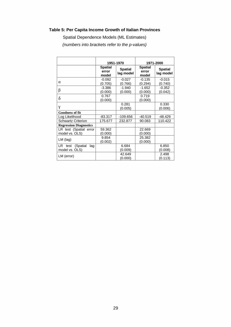
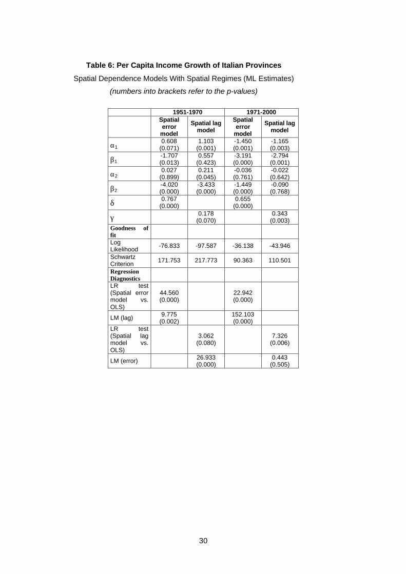
Tables 5 and 6 display the results of maximum likelihood estimates of spatial
error and spatial lag models for the two periods, respectively under the hypothesis of
unique and double regime.8 The parameters associated with the spatial error and the
spatial lag terms are always highly significant. This confirms the pronounced pattern of
spatial clustering for growth rates found in Section 3.1 by looking at the Moran’s I
statistics.
Table 5
the period 1951-1970 even some provinces belonging to central (Lazio, Umbria, Marche, Toscana) and North-Eastern (Friuli Venezia Giulia, Veneto) regions. On the other hand, some large southern provinces such as Napoli, Sassari, Palermo and Cagliari are included in the second regime. 8 An OLS cross-regressive model, which includes a spatial lag of the initial per capita income level, has been also tested for each period and for different specifications. The coefficient of this variable, however, was never found to be significant. In fact the diagnostics indicate that there is significant spatial dependence remaining in the cross-regressive model.
14
Table 6
Let us focus our attention on table 6 (spatial regimes). The fit of the spatial error
model (based on the values of Schwartz Criterion) is always higher than that of both
OLS and maximum likelihood spatial lag models. The spatial lag model outperforms the
OLS model only for the second period. Furthermore, the spatial diagnostics (LM and
LR tests) suggests that for the second period the spatial lag model is more reliable than
the spatial error model. As a consequence, the spatial error model with spatial regimes
must be regarded as the most appropriate specification for the first period; while the
spatial lag model with spatial regimes must be regarded as the most appropriate
specification for the second period. Compared to the OLS estimates, the initial per
capita income coefficients and the implied convergence rates did largely remained the
same for the second sub-period. Conversely, they increased for the first period (the one
of fast convergence).
In conclusion, the results reported in Tables from 1 to 6 provide strong evidence
of spatial effects in the unconditional convergence model widely applied in the
literature. These effects have some important implications in terms of the estimated
convergence speed. In particular, our results clearly suggest that, in the presence of a
strong positive spatial autocorrelation both in the per capita income levels and in the
growth rates, the OLS rate of convergence is strongly under-estimated and this in turn is
due to the fact that regional spill-over effects (knowledge is diffused over time through
cross region interaction) allow regions to grow faster than one would expect. Indeed, in
the presence of significant spatial error dependence, the random shocks to a specific
province are propagated throughout the country. The introduction of a positive shock to
the error for a specific province has obviously the largest relative impact (in terms of
growth rate) on this province. However, there is also a spatial propagation of this shock
to the other provinces. The magnitude of the shock spill-over dampens as the focus
moves away from the immediate neighbouring provinces (see also Rey and Montoury,
1998).
However, the coexistence of spatial dependence and spatial regimes9 implies that
there is a stumbling block to the knowledge diffusion: the formation of economies in
9 Controlling for spatial dependence in the b convergence approach does not eliminate the evidence of spatial regimes.
15
clusters according to interaction means that knowledge does not spill outside the cluster,
hence generating club convergence.
4. Intra-distribution dynamics and spatial effects
4.1 Stochastic kernel estimates
The spatial econometric approach used so far represents a very important tool to
control for the effects of spatial dependence and spatial heterogeneity. However, the β-
convergence approach has been strongly criticised on the ground that it suppresses the
very cross-section income dynamics one wishes to investigate. Generally speaking, a
negative association between growth rates and initial conditions can be consistent with a
rising, a declining and a stationary cross-section income dispersion. A method that
cannot differentiate between convergence, divergence or stationarity loses its validity on
testing ground. This failure is essentially a simple intuition of what is termed Galton’s
fallacy (Quah, 1993). The limits of the σ-convergence approach have been already
discussed in section 2.1.
Because of the limits of the σ- and β-convergence approaches, the last generation
of empirical growth studies has departed from the standard techniques of econometric
analysis, adopting an approach aimed at estimating the whole income dynamics rather
than just fitting the first two moments and thus revealing the evolution of income
distribution. In particular, according to Quah (1993, 1996a-b, 1997) the convergence
study must be based on the examination of shape and dynamics of the distribution.
For the evaluation of the first of the two aspects, that is the shape of the
distribution, it is possible to use nonparametric techniques of estimation of the
univariate density function. The advantage consists on less rigidity of the starting
hypotheses, so that, as Silverman (1985) said, “the data speak themselves”.
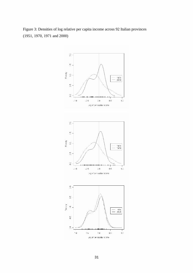
Figure 3 shows a sequence of kernel-smoothed densities of log-relative per capita
incomes across the 92 Italian provinces (i.e. the natural logarithm of the ratio between
the province’s income and the national average) taken at different points in time. The
16
kernel-smoothed estimates are obtained using a Gaussian Kernel with normal optimal
bandwidths chosen according to the mean squared error criteria.10
Figure 3
To better understand this figure, note that -0.5 on the horizontal axis corresponds
to half of the national average income, 0.0 indicates the national average and so on. The
height of the curve over any point gives the probability for any province to have that
relative rate. Thus, the area under the curve between -1.0 and 0.0 gives the total
likelihood for a province to have a relative per capita income equal to or lower than the
national average. In 1951, the income distribution appears very asymmetric (a positive
skewness is clearly shown): there are few relatively rich provinces and a lot of relatively
poor provinces. In 1970 a nascent twin-peakdness is being to be visible. In 2000, the
first peak appears more pronounced: there is a clustering together of the very rich and a
clustering together of the very poor. These results confirm the shape dynamics
underlying the hypothesis of “convergence clubs”.
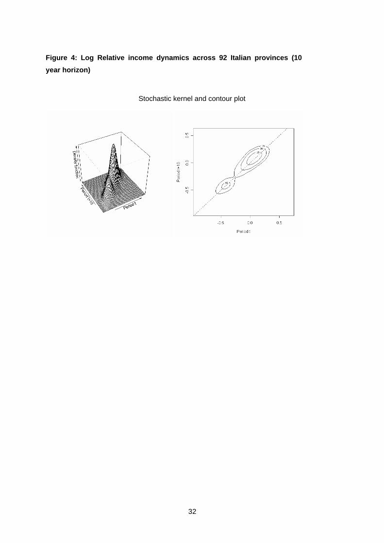
Let’s now turn to the mobility dynamics. A way to quantify the intra-distribution
dynamics is the bivariate kernel which estimates the joint density of the income
distribution at time t and t+10 (Figure 4). From any point on the axis marked Period t
extending parallel to the axis marked Period t+10 the stochastic kernel is a probability
density function. Roughly speaking, this probability density describes transitions over
10 years from a given income value in period t. Such a representation is equivalent to a
transition probability matrix with a continuum of rows and columns. It describes how
the cross-sectional distribution at time t evolves into that at t+10. Figure 4 confirms the
idea, suggested by the parametric analysis, that over the fifty years considered the
regional growth pattern in Italy has followed a polarisation process rather than a global
convergence path. The probability density mass is concentrated along the 45-degree
diagonal: elements in the distribution remain where they began. Moreover, a twin-peaks
property again manifests (contour plot makes this clearer). This is a confirmation that
10 The kernel estimator is a smoothed version of the histogram used to estimate a probability density function f of a random variable X (e.g. income). The estimator can be expressed as
( ) ∑=
−=
n
i
i
hXx
Knh
xf1
1 , where n is the number of finite observations in x; h is the smoothing
parameter called the bandwidth; and K is the kernel function of the variable x which can adopt various functions.
17
there exists clustering of economies into clubs at the neighbourhood of their initial
income groups.
Figure 4
4.2 Spatial conditioning
The emerging twin-peaks picture in Figure 4 is an instance of what Quah (1997)
calls “unconditional dynamics”. This author also proposes a method to “explain”
distribution dynamics, which is very different “from discovering a particular coefficient
to be significant in a regression of a dependent variable on some right-hand side
variables” (p. 44), as we performed in the previous section. This method is called
“conditioning”: it is based on “an empirical computation that helps us understand the
law of motion in an entire distribution” (p.44).
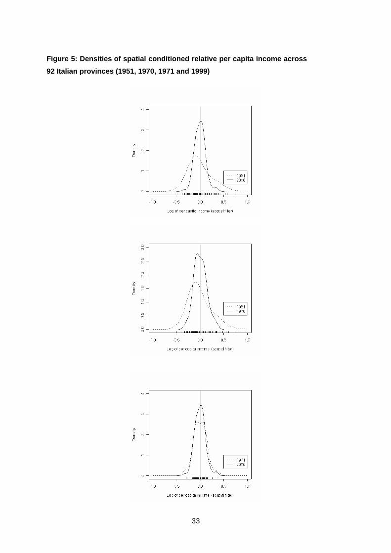
A conditioning schemes is articulated in two steps. Firstly, a spatially filtered
variable of each province per capita income is constructed.11 The filtered variable can be
interpreted as that part of income of each province which is not explained by the
spillover effects from the contiguous provinces. Then, with nonparametric analyses the
actual and the conditioned distributions are compared. The idea is that if inter-regional
spill-overs play a key role in the regional growth process, the spatial filtering removes
the twin-peaks features observed in the unconditional distribution of income.
Conversely, if the spatial contiguity is not influent, the distribution of the transformed
variable maintains its original characteristics: the polarisation can not be explained in
terms of spatially concentrated spill-overs.
The snapshot densities for the filtered variables displayed in Figure 5 no longer
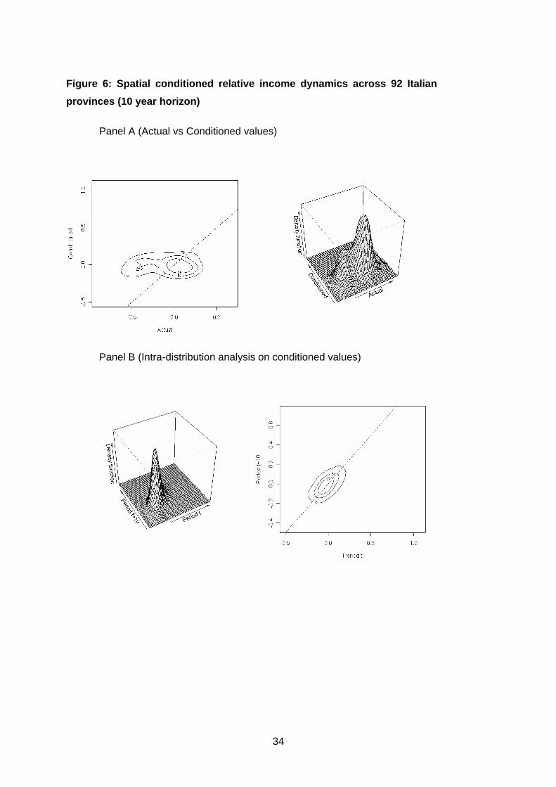
show emerging twin-peaks features. The relation between the actual and the conditioned
distributions is represented in Figure 6 (Panel A). Differently from Figure 4, we can
observe a counter-clockwise shift in mass to parallel the Original axis, as well as a
dissolving of twin-peaks. Finally, Figure 6 (Panel B) shows how the cross-sectional
distribution of the filtered income at time t evolves into that at time t+10. The evidence
11 The filtered variable is the ratio of per capita income to weighted average neighbourhood income:
∑=
jjj
ii y
yy
ϖ~ .
18
suggests that conditioning each province’s observation on the behaviour of its
neighbours, the income distribution collapses over time to a degenerate point limit: most
of the mass in the graph is concentrated around the national average value (0.0) of the
period t+10 axis. There is no more evidence of polarisation. Thus, one might say that
the polarisation earlier identified in the unconditional distribution-dynamics of cross-
province incomes is “well-explained” by physical geography. Not only are rich
provinces located close to other rich ones, such tendencies have magnified through
time.
To sum up, the unconditional dynamics of Italian province income data strongly
confirm the idea of polarisation (the convergence club hypothesis): poor provinces are
not catching up with rich ones; rather, there is a clustering together of the very rich, a
clustering together of the very poor and a vanishing of the middle class. Moreover,
spatial factors account for a large part of the distribution of incomes across provinces:
the spatial filtering removes the features of the unconditional dynamics. This confirms
that spillover and convergence clubs are spatially concentrated: most interaction and
exchange occur within groups of provinces physically close to one another (rich
provinces are typically close to – interact more with – other rich ones; similarly poor
economies are typically close to other poor ones). Without spillover effects, the
probability for a province to migrate from one to another an income class and to
converge towards an average value increases.
5. Concluding remarks
In the present paper we have examined the importance of spatial dependence and
spatial heterogeneity amongst data in estimating the convergence process of regional
per capita incomes, exploring both the β-convergence and stochastic kernel approaches.
Concerning the β-convergence approach, we have shown that, by examining the time
evolution of per capita incomes of the 92 Italian provinces (European NUTS-3 Regions)
in the period 1951-2000, neglecting the spatial nature of data leads both to a
misspecification of the growth model and to severe underestimation of convergence
rates. Firstly, the evidence of two spatial regimes in both periods suggests that
convergence occurred only among sub-groups of regions. Precisely, in the first period
(1951-70) only “relatively high income” regions follow a convergence path; in the
19
second period (1971-2000) only “relatively low income” regions show convergence.
Secondly, in the period examined, income levels and growth rates are characterised by a
strong spatial correlation, thus showing the presence of strong regional interdependence
and spill-overs. As a consequence, a region experiencing growth propagates positive
effects onto the neighbouring regions thus producing an acceleration of the convergence
process. By taking this element into consideration the rate of convergence calculated by
means of OLS results appear strongly underestimated. In the period 1951-70, the
standard OLS analysis suggests a speed of convergence among “relatively high income”
regions of 5.9%, whereas our spatially corrected models suggest a value of 7.3%. In the
second sub-period (1971-2000) the speed of convergence among “relatively low
income” regions is 4.9%, if estimated with the OLS, and rises up to 5.6% in the proper
spatial modelling specification.
Moving on to a kernel density approach, we have considered the shape dynamics
and mobility analysis associated with our data set and shown that inter-regional spill-
over play a crucial role in the analysis of growth processes and convergence. In fact the
twin-peak feature which is displayed by the data (consistent with other authors’
findings) is removed by a procedure of spatial filtering. In this way our study, while
confirming a convergence club hypothesis for Italy 1951-2000, shows that these clubs
are spatially concentrated and this effect reduces the probability of converging by
migrating from one income class to the other.
The present results are of paramount importance in terms of policy evaluation and
suggest that spatial effects captured by the models presented here are important
elements to be considered in targeting resources.
The analysis reported here is preliminary in many respects. First of all, the
convergence analysis carried out here uses data in the per capita income. Yet growth
theories make predictions about labour productivity not income! Growth models
concentrate on aggregate production function and assume full employment. Thus, they
make no predictions about unemployment and labour force participation. As it was
suggested elsewhere (e.g. Boldrin and Canova, 2001) this makes all the difference in the
empirical analysis. Indeed, the observed inequalities at the provincial level can be due to
the combination of three factors namely: i) differences in labour productivity, ii)
differences in employment rates, and iii) interactions between productivity and
employment rates. In a future paper, we will address this aspect by looking at a recently
20
compiled database on labour productivity and employment rates for the 95 Italian
provinces.
Secondly, in the present paper we have not considered the effect of explanatory
variables other than the initial income level. Future research effort should move towards
the testing for the presence of conditional convergence by introducing into
consideration conditioning variables like human capital and infrastructure in the
presence of spatial dependence.
Finally, the non parametric approach initially considered here can be extended in
order to include other conditional factors different from the simple spatial contiguity.
Furthermore the provisional hypotheses set out in this paper could be validated using
different empirical data.
References Anselin L. (1988), Spatial econometrics, Kluwer Academic Publishers, Dordrecht.
Anselin L. and A.K. Bera (1998), Spatial dependence in linear regression models with an introduction to spatial econometrics, in Hullah A. and D.E.A. Gelis (eds.) Handbook of Applied Economic Statistic, Marcel Deker, New Jork, pp. 237-290.
Anselin L. and S.J. Rey (1991), Properties of test for spatial dependence, Geographical Analysis, 23, 2, pp. 112-131.
Arbia G. (1988), Spatial data configuration in statistical analysis of regional economic and related problems, Kluwer Academic Publisher, Dordrecht.
Arbia G. (2000), Two critiques to the statistical measures of spatial concentration and regional convergence, International Advances in Economic Research, 6, 3, August.
Arbia G. (2001), The role of spatial effects in the empirical analysis of regional concentration, Journal of Geographical systems, 3, pp. 271-281.
Arbia G. and J.H.P. Paelinck (2002), Which way to equality? A continuous time modelling of regional convergence, Paper presented at the European Regional Science Association, August 27 - 31 2002 Dortmund (Germany).
Barro R.J. and X. Sala-i-Martin (1992), Convergence, Journal of Political Economy, 100, pp. 223-251.
Barro R.J. and X. Sala-i-Martin (1995), Economic Growth, McGraw Hill, New York.
Boldrin M. and F. Canova (2001), Europe’s Regions: Income Disparities and Regional Policies, Economic Policy, 32, pp. 207-53.
Cellini R. and A. Scorcu (1995), How Many Italies?, Università di Cagliari, mimeo.
Cliff A.D. and J. K. Ord (1973), Spatial autocorrelation, Pion, London. Cleveland W.S. (1979), Robust Locally-Weighted Regression and Scatterplot
Smoothing”, Journal of the American Statistical Association, n.74.
21
Cleveland W.S. and S.J. Devlin (1988), Locally-Weighted Regression: an Approach to Regression Analysis by Local Fitting, Journal of the American Statistical Association, n.83.
Conley T. (1999), GMM estimation with cross sectional dependence, Journal of Econometrics, 92, 1, pp. 1-45.
Cosci S. and F. Mattesini (1995), Convergenza e crescita in Italia: un’analisi su dati provinciali, Rivista di Politica Economica, 85, 4, pp. 35-68.
Durlauf S.N., A. Kourtellos and A. Minkin (2001), The Local Solow Growth Model, European Economic Review, n. 45.
Durlauf S.N. and D.T. Quah (1999), The New Empirics of Economic Growth, in J.B. Taylor e M. Woodford (eds.), Handbook of Macroeconomics, vol. IA, Cap. 4, North-Holland, Amsterdam.
Durlauf S.N. and P. Johnson (1995), Multiple Regimes and Cross-Country Growth Behavior, Journal of Applied Econometrics, n. 10.
Fabiani S. and G. Pellegrini (1997), Education, Infrastructure, Geography and Growth: an Empirical Analysis of the Development of Italian Provinces, Temi di discussione, Bank of Italy, Rome.
Hansen B. (1996), Sample Splitting and Threshold Estimation, mimeo.
Liu Z. and T. Stengos (1999), Non-Linearities in Cross-Country Growth Regressions: a Semiparametric Approach, Journal of Applied Econometrics, n. 14.
Mankiw N. G., Romer D. and D.N. Weil (1992), A contribution to the empirics of economic growth, Quarterly Journal of economics, May, pp. 407-437.
Paci R. and F. Pigliaru (1995), Differenziali di crescita tra le regioni italiane: un’analisi cross-section, Rivista di Politica Economica, 85, 10, pp. 3-34.
Quah D. (1993), Galton’s Fallacy and Test of the Convergence Hypothesis, The Scandinavian Journal of Economics, n. 4.
Quah D. (1996a), Regional convergence clusters across Europe, European Economic Review, 40, pp. 951-958.
Quah D. (1996b), Empirics for economic growth and convergence, European Economic Review, 40, 6, pp. 1353-7.
Quah D. (1997), Empirics for growth and distribution: stratification, polarization, and convergence clubs, Journal of Economic Growth, 2, pp. 27-59.
Rey S.J. (2000), Spatial empirics for economic growth and convergence, Working Papers of San Diego State University.
Rey S.J. and B.D. Montouri (1998), US regional income convergence: a spatial econometric perspective, Regional Studies, 33, 2, pp. 143-156.
Silverman, B.W. (1985), Some aspects of the spline smoothing approach to nonparametric regression curve fitting. Journal of Royal Statistical Society, Ser. B 47, pp. 1–52.
Solow R.M. (1956), A contribution to the theory of economic growth, Quarterly journal of economics, LXX, pp. 65-94.
Swan T.W. (1956), Economic growth and capital accumulation, Economic Record, 32, November, pp. 334-361.
Acknowledgements
22
We wish to thank the participants at the 17th Annual Congress of the European
Economic Association (EEA) Venice, August 22nd - 24th, 2002, for the useful comments
on a previous version of the paper. We wish also to thank Massimo Guagnini for kindly
providing the data used in the paper.
23
Figure 1: Italian provinces convergence of per-capita income and related spatial autocorrelation in the period 1951-2000
Table 4: Per Capita Income Growth of Italian Provinces
Spatial Regime Models - OLS Estimates
(numbers into brackets refer to the p-values)
1951-1970 1971-2000
α1 1.257
(0.001) -1.246 (0.004)
β1 0.719
(0.306) -2.646 (0.006)
α2 0.287
(0.009) 0.017
(0.739)
β2 -3.604 (0.000)
-0.181 (0.588)
Goodness of fit Adjusted R2 0.560 0.080 Log-likelihood -99.113 -47.610 Schwartz Criterion 216.314 113.306 Regression Diagnostics
Jarque-Bera 4.367 (0.112)
3.977 (0.137)
Moran’s I 5.522 (0.000)
3.264 (0.001)
LM (error) 25.250 (0.000)
8.005 (0.004)
LM (lag) 3.224 (0.072)
7.946 (0.005)
29
Table 5: Per Capita Income Growth of Italian Provinces
Spatial Dependence Models (ML Estimates)
(numbers into brackets refer to the p-values)
1951-1970
1971-2000
Spatial error
model
Spatial lag model
Spatial error
model
Spatial lag model
α -0.092 (0.705)
-0.027 (0.766)
-0.135 (0.294)
-0.015 (0.740)
β -3.386 (0.000)
-1.940 (0.000)
-1.652 (0.000)
-0.352 (0.042)
δ 0.767 (0.000) 0.719
(0.000)
γ 0.281 (0.005) 0.330
(0.006) Goodness of fit Log Likelihood -83.317 -109.656 -40.519 -48.429 Schwartz Criterion 175.677 232.877 90.083 110.422 Regression Diagnostics LR test (Spatial error model vs. OLS)
59.362 (0.000) 22.669
(0.000)
LM (lag) 9.854 (0.002) 25.382
(0.000)
LR test (Spatial lag model vs. OLS) 6.684
(0.009) 6.850 (0.008)
LM (error) 42.649 (0.000) 2.498
(0.113)
30
Table 6: Per Capita Income Growth of Italian Provinces
Spatial Dependence Models With Spatial Regimes (ML Estimates)
(numbers into brackets refer to the p-values)
1951-1970 1971-2000
Spatial error
model
Spatial lag model
Spatial error
model
Spatial lag model
α1 0.608
(0.071) 1.103
(0.001) -1.450 (0.001)
-1.165 (0.003)
β1 -1.707 (0.013)
0.557 (0.423)
-3.191 (0.000)
-2.794 (0.001)
α2 0.027
(0.899) 0.211
(0.045) -0.036 (0.761)
-0.022 (0.642)
β2 -4.020 (0.000)
-3.433 (0.000)
-1.449 (0.000)
-0.090 (0.768)
δ 0.767 (0.000) 0.655
(0.000)
γ 0.178 (0.070) 0.343
(0.003) Goodness of fit
Log Likelihood -76.833 -97.587 -36.138 -43.946
Schwartz Criterion 171.753 217.773 90.363 110.501
Regression Diagnostics
LR test (Spatial error model vs. OLS)
44.560 (0.000) 22.942
(0.000)
LM (lag) 9.775 (0.002) 152.103
(0.000)
LR test (Spatial lag model vs. OLS)
3.062 (0.080) 7.326
(0.006)
LM (error) 26.933 (0.000) 0.443
(0.505)
31
Figure 3: Densities of log relative per capita income across 92 Italian provinces
(1951, 1970, 1971 and 2000)
32
Figure 4: Log Relative income dynamics across 92 Italian provinces (10
year horizon)
Stochastic kernel and contour plot
33
Figure 5: Densities of spatial conditioned relative per capita income across
92 Italian provinces (1951, 1970, 1971 and 1999)
34
Figure 6: Spatial conditioned relative income dynamics across 92 Italian
provinces (10 year horizon)
Panel A (Actual vs Conditioned values)
Panel B (Intra-distribution analysis on conditioned values)