United States Policy, Planning EPA-230-10-89-069 Environmental Protection and Evaluation October 1989 Agency (2127) Measuring the Benefits of Water Quality Improvements Using Recreation Demand Models: Part I
Transcript
United States Policy, Planning EPA-230-10-89-069Environmental Protection and Evaluation October 1989Agency (2127)
Measuring the Benefits ofWater Quality ImprovementsUsing Recreation Demand Models: Part I
MEASURING THE BENEFITS
OF WATER QUALITY IMPROVEMENTS
USING RECREATION DEMAND MODELS
Volume II
of
BENEFIT ANALYSIS USING
INDIRECT OR IMPUTED MARKET METHODS
Prepared and Edited by
Nancy E. B o c k s t a e l University of Maryland
W. Michael HanemannUniversity of California
Ivar E. Strand, Jr.University of Maryland
Principal Investigators
Kenneth E. McConnell and Nancy E. BockstaelAgricultural and Resource Economics
University bf Maryland
EPA Contract No. CR-811043-O1-O
Project Officer
Dr. Alan CarlinOffice of Policy Analysis
Office of Policy and Resource ManagementU. S. Environmental Protection Agency
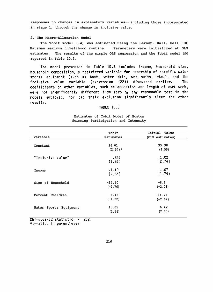
Washington, D.C. 20460
The information in this document has been funded wholly or inpart by the United States Environmental Protection Agencyunder Cooperative Agreement No. 811043-01-0. It has beensubjected to the Agency’s peer and administrative review, andhas been approved for publication as an EPA document. Mentionof trade names or commercial products does not constituteendorsement or recommendation for use.
ACKNOWLEDGEMENTS
Kenneth E. McConnell, Terrence P. Smith, and Catherine L. Kling weremajor contributors to this volume, providing both original contributions andbeneficial comments. The authors have also benefited from comments of EPAstaff members, including Peter Caulkins and George Parsons, and fromreviewers Edward Morey and Clifford Russell. Technical assistance wasprovided by Jeffrey Cunningham and Chester Hall. Additionally, both creditand appreciation are due Alan Carlin, our project officer in the BenefitsStaff of EPA. Throughout the research, Diane Walbesser supplied invaluablesecretarial and technical assistance. Finally, Linda Griffin of ADEAWordprocessing and Patricia Sinclair of the University of Maryland deservespecial thanks for undertaking the arduous task of typing this manuscript.
All opinions and remaining errors are the sole responsibility of theeditors. This effort was funded by US EPA Cooperative Agreement number CR-811043-01-0.
FOREWARD
This is the second of two volumes constituting the final report forbudget period I of Cooperative Agreement #811043-01-0, which was initiatedand supported by the Benefits Staff in the Office of Policy Analysis at theU.S. Environmental Protection Agency (EPA). The two volumes, whi1e encom-passed under the same cooperative agreement, are distinct in nature. Thetopic of Volume 11 is the use of recreational demand models in estimatingthe benefits of water quality improvements.
The research reported here is the result of interaction among theprincipal investigators of the project, the editors of the volume,individual contributors at the University of Maryland, and outsidereviewers. In addition to the team of editors, Kenneth E. McConnell,Terrence P. Smith, and Catherine L. Kling were major contributors, providingboth original research and invaluable review.
The editors benefited considerably from comments by outside reviewers,Edward Morey of University of Colorado and Clifford Russell, now ofVanderbilt University. Important contributions were also made by EPA staffincluding Alan Carlin, Peter Caulkins, George Parsons and Walter Milon. Itwould be impossible to cite all the individuals who had an influence on theideas presented here, but two of these must be mentioned, V. Kerry Smith ofVanderbilt University and Richard Bishop of the University of Wisconsin.
Progress made in this volume toward the resolution of the problems anddilemmas which plague the assessment of environmental quality improvementsmust be attributed to a wide range of sources. In large part the workreflects the cumulative efforts of a decade or two of researchers in thisarea. And, it is itself merely a transitionary stage in the development andsynthesis of the answers to those problems. More progress has already beenmade on many of these issues - both by the authors and by other economistsworking in the field. This new work will be reflected in future cooperativeagreement
Also,analysisdesignedTriangle
reports.
included in the next budget period’s report will be discussion andof survey data collected during budget period I. The survey,by Strand, McConnell and Bockstael in conjunction with ResearchInstitute (RTI), was administered by RTI. It includes a telephone
survey of households in the Baltimore-Washington SMSA’s and a field surveyconducted during the summer of 1984 at public beaches on the Western shoreof the Chesapeake Bay. The survey provides data on swimming behavior whichis being analyzed using some of the developments discussed in this volume.The survey instrument, the data, and the analysis will be presented in thenext cooperative agreement report.
EXECUTIVE SUMMARY
In an era of growing Federal accountability, those programs whichcannot substantiate returns commensurate with budgets are severely disadvan-taged. Expressions such as Executive Order 12291 require an. account of thebenefits of public interventions. Inability to provide, or inaccuracy inthe provision of, those estimates undermines the credibility of programs andmay cause their untimely demise.
The public provision of improvements in water quality is an activityendangered by the complexities involved in the accounting of benefits. Thelack of markets and observed prices in water-related recreational activityhas necessitated the use of surrogate prices in benefit assessment. More-over, a formal regime (i.e. The Principles and Standards for Water Quality)articulates the assessment procedure. Unfortunately, the regime still con-tains ambiguities, inconsistencies and slippage sufficient to raise poten-tial controversy over any estimate of benefits from water qualityimprovements.
The purpose of Volume 11 is to address some of those ambiguities andinconsistencies and, in so doing, provide a more comprehensive, credibleapproach to the valuation of benefits from water quality improvements.Substantial progress is made in improving valuation techniques by linkingthe fundamental concepts of the “travel cost” model with cutting-edgeadvances in the labor supply, welfare, and econometrics literature.
At the heart of the research is the study of individual recreationbehavior. As water quality improves, individual behavior changes,reflecting improvements in welfare. Misconceptions and inaccuracies may’arise if benefit evaluations are based on inappropriate aggregation ofindividual’s behavior. An analysis of the “zonal” (an aggregate) approachrepresents one contribution of Volume II. Alternatives to the zonalapproach are offered. The new approaches are based on advances in thestatistical analysis of limited dependent variables.
The realities of recreational choice encompass more dimensions thantraditional demand analysis. Time is critical - over 50% of respondents ina recent national survey replied that “not enough time” was the reason theydid not participate more often in their favorite recreation, while only 20%replied “not enough money.” Drawing on labor supply literature, an exten-sion of traditional demand analysis to include time constraints is developedin Volume XI. The extension, which is made operational, captures the truenature of recreational decisions which are affected as much by individuals’time constraints as their money constraints.
Statistical analysis is emphasized throughout the volume. One exampleis an examination of the properties of welfare estimates. Because typicalwelfare estimates are derived from numbers with random components, they haverandom components themselves. Thus it is important to study the statisticalproperties of typically used estimators for welfare measures. These proper-ties, such as biasedness, are shown to be undesirable in several instances.More credible estimators are provided. Another statistical issue, causes ofrandomness in estimates, is shown to influence the magnitude of welfareestimates. Ways in which information about the source of randomness can beused to improve accuracy are discussed.
Part II of Volume addresses problems specifically associated withintroducing aspects of water quality into the fundamental model developed inPart I. The desire to incorporate environmental characteristics (such aswater quality) has prompted the treatment of an additional dimension to therecreational model. Data collected for one recreational site do not, bytheir nature, exhibit variation in the quality characteristics of that site,preventing the researcher from deducing anything about how demand changeswith changes in quality characteristics. The only reliable means ofincorporating quality is to model the demand for an array of sites ofdiffering qualities. However, the need to develop models of multiple sitedecisions has been a blessing in disguise, for it has forced modelers torecognize that recreational decisions are frequently made among an array ofcompeting, quality-differentiated resources.
A major share of Part II of this volume is devoted to the discussion ofmodels which can incorporate quality characteristics in multiple site recre-ational demand decisions. While a theoretically consistent model can bedeveloped, it is not empirically feasible, and several second best modelsare presented. Criteria for evaluating these alternative models includestheir ability to capture the nature of recreational decisions and to respondto the research goal of valuing environmental quality changes.
vi
TABLE OF CONTENTS
Part I
ADVANCES IN THE USE OF RECREATIONAL DEMAND MODELS FOR BENEFIT VALUATION
Appendix 2.1 DERIVATION OF SOME UTILITY THEORETIC MEASURES FROM . . . . . . ...29TWO GOOD DEMAND SYSTEMS
Appendix 2.2 COMPUTER ALGORITHM FOR OBTAINING COMPENSATING AND . . . . . . . . ...33EQUIVALENT VARIATION MEASURES FROM ESTIMATEDMARSHALLIAN DEMAND FUNCTIONS
Chapter 3 AGGREGATION ISSUES: THE CHOICE AMONG ESTIMATION . . . . . . . . . ...35APPROACHES
A Review of Past Literature . . . . . . . 361. The Zonal Approach . . . . . . . . . ● . ● 362. The Individual Observation Approach . . . . . . . . . . . . . . . 4O
vii
TABLE OF CONTENTS (continued)
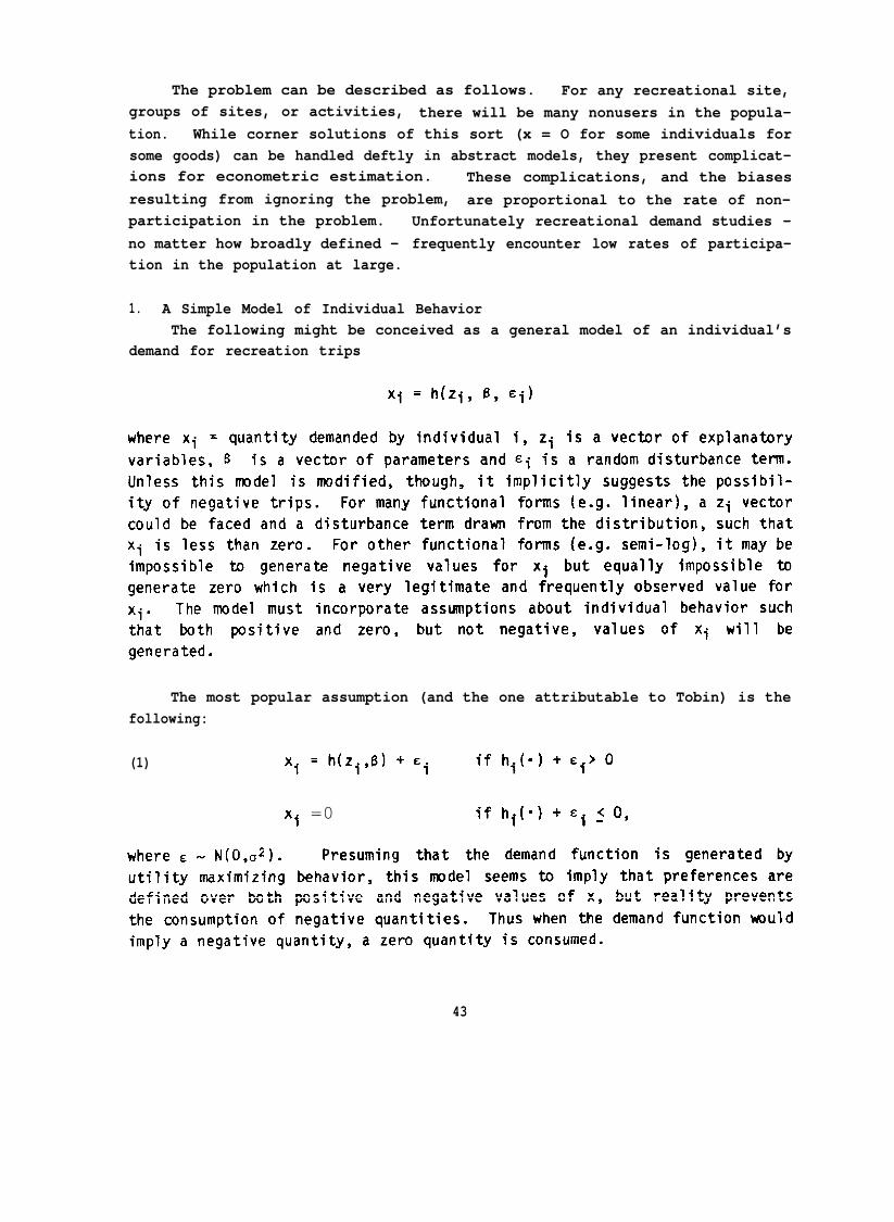
Models of Individual Behavior and Their Implications . . . . . ...42for Estimation1. A Simple Model of Individual Behavior . . . . . . . . . . . . . ...432. A Model of Behavior When Different Variables . . . . . ...46
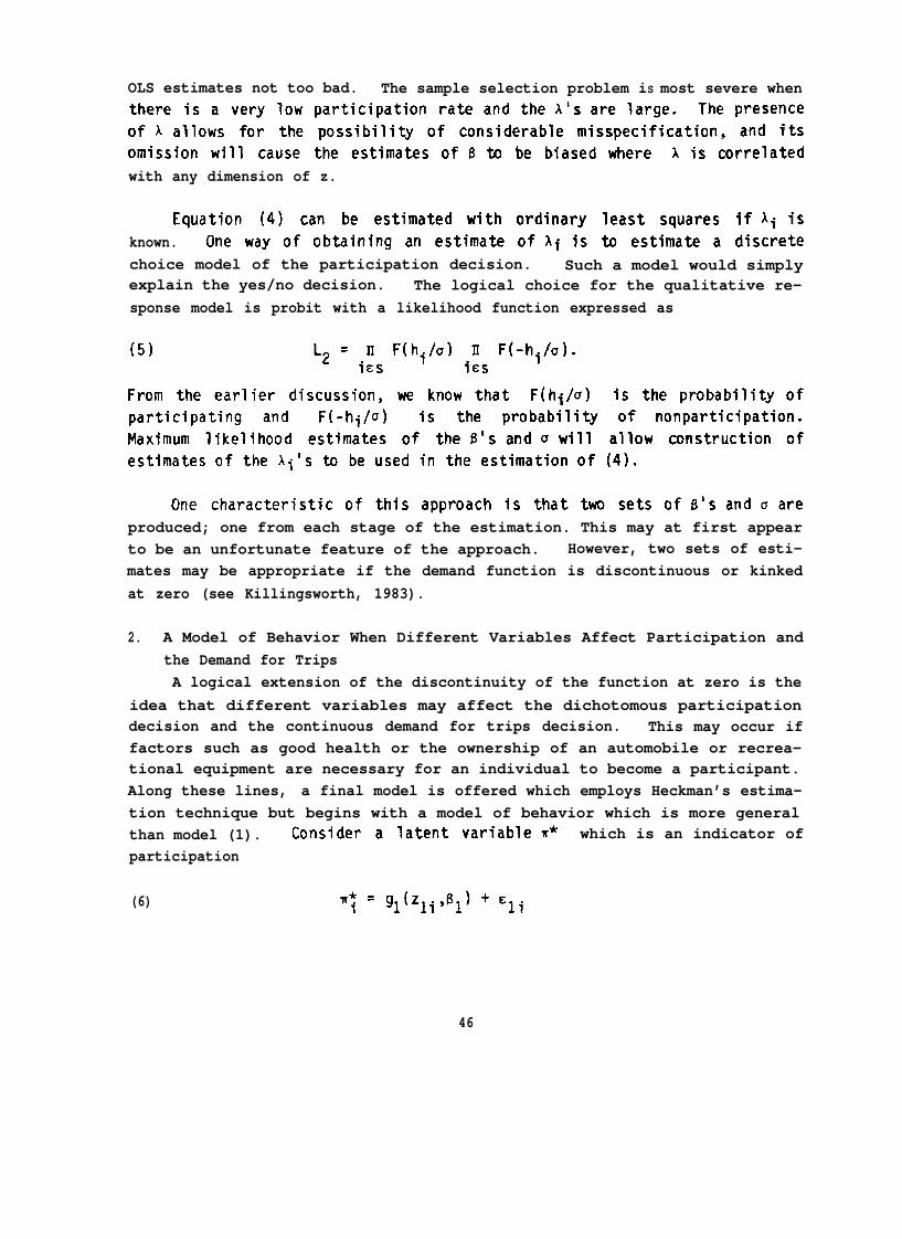
Affect Participation and the Demand for Trips3. Estimation When the Sample Includes Only . . . . . . . . . . ...47
Appendix 5.1 DERIVATION OF DIFFERENCES IN ESTIMATED CONSUMER . . . . . . . . . ...112SURPLUS USING THE SEMI-LOG DEMAND FUNCTION
viii
TABLE OF CONTENTS
Part II
MULTIPLE SITE DEMAND MODELS AND THE MEASUREMENT OF BENEFITS FROMWATER QUALITY IMPROVEMENTS
Chapter 6 RECREATION DEMAND MODELS AND THE BENEFITS FROM . . . . . . . . . . ...115IMPROVEMENTS IN WATER QUALITY
Valuing Quality Changes in Demand Models . . . . . . . . . . . . . . . . . ..ll6Extending the Single Site Model to Value Quality Changes...ll7Plan of Research for Part II . . . .119
Chapter 7 EVALUATING ENVIRONMENTAL QUALITY IN THE CONTEXT . . . . . . ... ..l20OF RECREATIONAL DEMAND MODELS: AN INTRODUCTIONTO MULTIPLE SITE MODELS
The Nature of Recreation Demand ● ● ● ● ● ● ● ● ● ● ● ● ● ● ● ● 121Introducing Quality into the Demand Function . . . . . . . . . . . . . ..l22The Specification of Demand Models for Systems of . . . . . . . . ..l26
Volumes I and II of this report are the result of one year’s researchconducted under EPA Cooperative Agreement CR-811043-O1-O. The particularmethods designated by EPA to be of primary interest in this cooperativeagreement are “imputed or indirect market methods,” i.e. methods which de-
pend on observed behavior in related markets rather than direct hypotheticalquestioning. Despite their similar themes, the two volumes are distinct inmany respects. Volume I addresses a specific technical issue (the identifi-cation problem) associated with the hedonic method of valuing goods. Thesecond volume discusses a wider range of technical issues associated withthe use of recreational demand models to value environmental qualitychanges. The primary purpose of the agreement has been to develop anddemonstrate improved methods for estimating the regional benefits fromenvironmental improvements.
Within this volume dedicated to recreation demand models, Part I isrestricted to a set of issues which arise in benefit valuation using theconventional single site recreational model. The topic of Part 11 is theapplication of recreation demand models for the specific task of measuringthe benefits associated with changes in the quality of the recreationalexperience. Attention is given, in particular, to water quality improve-ments. In this spirit, Part II explores a broad range of models based onindividual behavior which can be used to reveal valuations of environmentalimprovements. These models attempt to establish the relationship betweenuse activities (specifically recreation) and water quality and can be usedto devise welfare measures to assess benefits.
The emphasis this volume gives to recreation behavior is not mis-placed. A 1979 report by Freeman (1979b) to the Council of EnvironmentalQuality estimated that over fifty percent of the returns from air and waterquality improvements would accrue through recreational uses of the envi-ronment. When considering water quality improvements alone, the percentagewas even higher. One of the earliest studies attempting to quantify such
effects (Federal Watertionists would receivequality improvements insupported by the U.S.
Pollution Control, 1966) estimated that recrea-more than 95% of the benefits derived from waterthe Delaware estuary. These sentiments were furtherNational Commission on Water Quality (1975) which
maintained that water based recreators would be the major beneficiaries ofthe 1972 Federal Water Pollution Control Act.
Thus, the emphasis in these two volumes is on recreation, but the tasksare wide-ranging. The initial charge in the Cooperative Agreement was abroad one, including the development of improved methods, the demonstrationof new techniques, the collection of primary data and the assessment of theusefulness of the resulting benefit estimates. The emphasis in this firstyear of work has been where it must be, on the first items in this list, al-though progress has been make on each task.
Nonmarket Benefit Evaluation and the Development of Methods
Despite the near consensus which currently exists in market-orientedwelfare theory (i.e. welfare changes in private markets), economists are farfrom embracing a complete methodology for valuing public (often environ-mental), non-market goods. It hardly seems necessary to document thiscontention. One need only consider some of the many recent conferenceswhich have attempted to resolve difficulties and increase consensus on theseissues, (e.g. Southern Natural Resource Economics Committee, Stoll, Shulstadand Smathers, 1983; Cummings, Brookshire and Schulze, 1984; EPA Morkshop onthe State of the Art in Contingent Valuation, and AERE Workshop on Valuationof Environmental Amenities, 1985.) In essence “Nonmarket valuation has along way yet to go before all the problems will be solved and its acceptanceby economists will be unequivocal (SNREC, p.4).”
The valuation exercise has been viewed by many economists as an attemptto bring nonmarket goods into policy considerations on a comparable footingwith private marketed goods. However, to be accurate, some economists andmany non-economists have questioned the relevancy of the market analogy forpublic good valuation. Arguments by philosophers include reference to asocial ethic and contend that societies may have collective values indepen-dent of individual preferences. Not so well articulated are our ownconcerns about how people think about public goods and how they relatepublic goods to private expenditures. To what extent can a change in apublic good be translated into an effect on an individual such that an indi-vidual’s willingness to pay is a meaningful concept?
2
The existence of rival theories and the lack of consensus we see in thenon-market benefits literature is not unlike the early stages of the de-velopment of other fields of economics and of other sciences. In the earlystages of a science or a subfield of a science, Thomas Kuhn has argued thatcompetition exists among a number of distinct views all somewhat arbitraryin their formulation. Eventually a set of theories, Kuhn’s now familiar“paradigm,” emerges which provides focus to future work. The paradigm isthe set of fundamental concepts and theories which all additional work takesas given. The eventual acceptance of a paradigm allows, and in fact en-courages, research to become more focused, more refined, and moredetailed. This body of accepted thought provides the necessary structureand standards of judgement without which research becomes confusion. Kuhn’sessential point was that the science could only be advanced in the contextof the paradigm.
Whether we wish to view it as a pre-paradigm stage or a crisis in theneoclassical paradigm, the development of what has become “traditional”welfare economics (i.e. welfare measurement in private markets) provides acase in point. Welfare economics has a long history of controversy, begin-ning with loosely defined and imprecisely measured concepts of rent andconsumer surplus extending as far back as Ricardo and Dupuit. The estab-lishment of these concepts as foundations of a theory of economic welfarewas a long and uphill battle involving attacks by new welfare economists onthe old welfare economics and the development of the compensation princi-ple. For a very long period the state of welfare economics was one ofcrisis, with applied economists pursuing empirical studies which theoreti-cians condemned. Over time, and with theoretical developments by economistssuch as Willig, Hausman, Just et al., Hanemann, and others, a theoreticalfoundation for feasible empirical practices has emerged in the form of the“willingness to pay” paradigm.
With the recognition that public policies frequently produce benefitsand losses outside of markets comes a new controversy and an attempt tostretch the existing “willingness to pay” paradigm to cover new ground. Tomany established economists, the problem seems straightforward: thevaluation of nonmarket benefits through benefit-cost analysis, under idealprocedures for extracting value measures, is assumed to provide the sameanswer that the market mechanism would provide. The major difficulties liein defining those ideal procedures. Some question whether these measuresexist, or are meaningful, in the context in which we wish to use them - i.e.
can the willingness-to-pay paradigm really be stretched and modified toresolve the anomalies which public good valuation present?
This subfield of economics, the valuation of public goods, is in aperiod of crisis in its development, but it is not unlike periods of crisiswhich have arisen in other areas of economics or in the natural and physicalsciences. Kuhn describes these periods as marked by debates over legitimatemethods, over relevant experiments, and over standards by which results canbe judged - a description which fits closely the current activities in non-market valuation. In these periods of crisis, Kuhn argues,and unarticulated theories develop which eventually pointcovery.
many speculativethe way to dis-
The implication of Kuhn’s thesis is that more refined and preciseanalysis either establishes a closer match between theory and observation orprovides more evidence that such a match does not exist. The only way todetermine whether standard welfare economics can be stretched to resolve thepublic good valuation problem is to explore nonmarket valuation problems ina rigorous welfare theoretic framework. If the anomalies can not be re-solved, even with increasingly careful modelling and precise measurement,then the balance will tip In favor of seeking a new paradigm. But it isonly in the context of some carefully conceived theoretical structure thatprogress can be made. “Truth emerges more readily from error than fromconfusion (Kuhn, 1969).”
Making Benefit Measures More Defensible
An attempt to apply scientific methods to nonmarket benefit analysisimmediately raises problems. Our approaches provide estimates of welfarefor which we have no direct observations for comparison. The absence ofdirect observation on welfare changes directly only suggests that welfaremeasures should be defined on models of behavior which can be observed.
Starting, as they do, from models of economic behavior, one would thinkthat welfare measures derived from models of observable behavior in marketsrelated to environmental goods (e.g. recreational demand models) would be apopular approach. Certainly, the travel cost approach, a specific variantof more general models of economic behavior, has produced many benefit esti-mates in its long life. Yet this approach’s credibility has been challengedon two counts.
First, policy makers argue that many amenities of interest can not beassociated closely enough with a market or with observable behavior to allowfor the use of related market methods. This criticism has some very impor-tant implications. On the pragmatic side, it is useful to note recent re-sults in contingent valuation assessment. Contingent valuation, the prin-ciple alternative method, has been pronounced quite reliable as long as thegood to be valued is closely related to a market experience. What is moregermane to the argument here is that when valuation is unrelated to observ-able behavior, it is impossible to test the predictions of theories againstobservations - and as a consequence we can have no confidence in those pre-dictions. In fact, it is unclear that economic valuation has any meaning ina context where there exists no related observable economic behavior. Weare reminded of Kuhn’s warning “measurements undertaken without a paradigmseldom lead to any conclusions at all.”
The second criticism of market related valuation approaches is that thesame valuation problem can generate a vast array of radically differentbenefit estimates. How can one trust a method which appears capable ofgenerating a number of very different answers to the same question?
If we examine the literature or conduct experiments ourselves, we in-evitably encounter this embarrassing problem: benefit estimates seem verysensitive to specification, estimation method, aggregation, etc. It is thecontention of the current work, however, that valuation methods based on be-havioral models allow the potential for resolving inconsistencies, since theapparent arbitrary choices we make about specification, etc. are really im-plicit but testable hypotheses about individual behavior. By being moreprecise about the behavioral assumptions of our models, more defensiblebenefit estimates can be defined.
The philosophy inherent in our research agenda is that if benefitmeasures are to be taken seriously by policy makers they must be based ondefensible, realistic models of human behavior. Perfect measures can not bedefined and will always be inaccessible. But arbitrariness in estimatinghuman behavior can be reduced by careful model specification and estimation,so that we know ultimately what assumptions are implicit in the benefitestimates as well as the direction of possible biases in these estimates.
This philosophy requires that we first assess the state of benefitestimation using indirect market methods and then attempt to make im-provements in those areas which seem either the most confused or the most
5
vulnerable. A goal of the current research is to bring together the manyrecent advances in recreational demand estimation, specifically, and appliedwelfare economics, more generally, to further the development of defensiblemodels of measuring water quality improvements.
One comment needs to be made with regard to alternative benefitmeasurement techniques. The arguments in this Chapter are not intended tochampion the cause of recreational demand models over contingent valuationtechniques. The purpose of this as well as other studies should be to improve the credibility of techniques for valuing environmental amenities. Itis our opinion that the science will be advanced if contingent valuation andindirect market methods are considered as complements. To the extent thatthe two approaches can be made comparable, their conjunctive use can onlystrengthen benefit estimation. While many studies have compared estimatesderived from the two approaches (e.g. Knetsch and Davis 1966; Bishop andHeberlein 1979; Thayer 1981), few have tried to relate the approaches con-ceptually and none have attempted to ensure that the underlying assumptionsof the models are consistent. The two approaches applied to the same cir-cumstances can potentially be made comparable since they are both the reali-zation of individual’s preferences subject to constraints. Just as thereare assumptions about behavior implicit in the way in which we specify andestimate recreational demand models, there are similar if less conspicuousassumptions implicit in the way contingent valuation experiments are framedand the way benefit estimates are derived from the hypothetical answers.While a means for making the two approaches comparable is beyond the scopeof this year’s project, future efforts in this direction will be rewarding.
The Empirical Foundation of Recreation Demand Models: The TraditionalTravel Cost Model
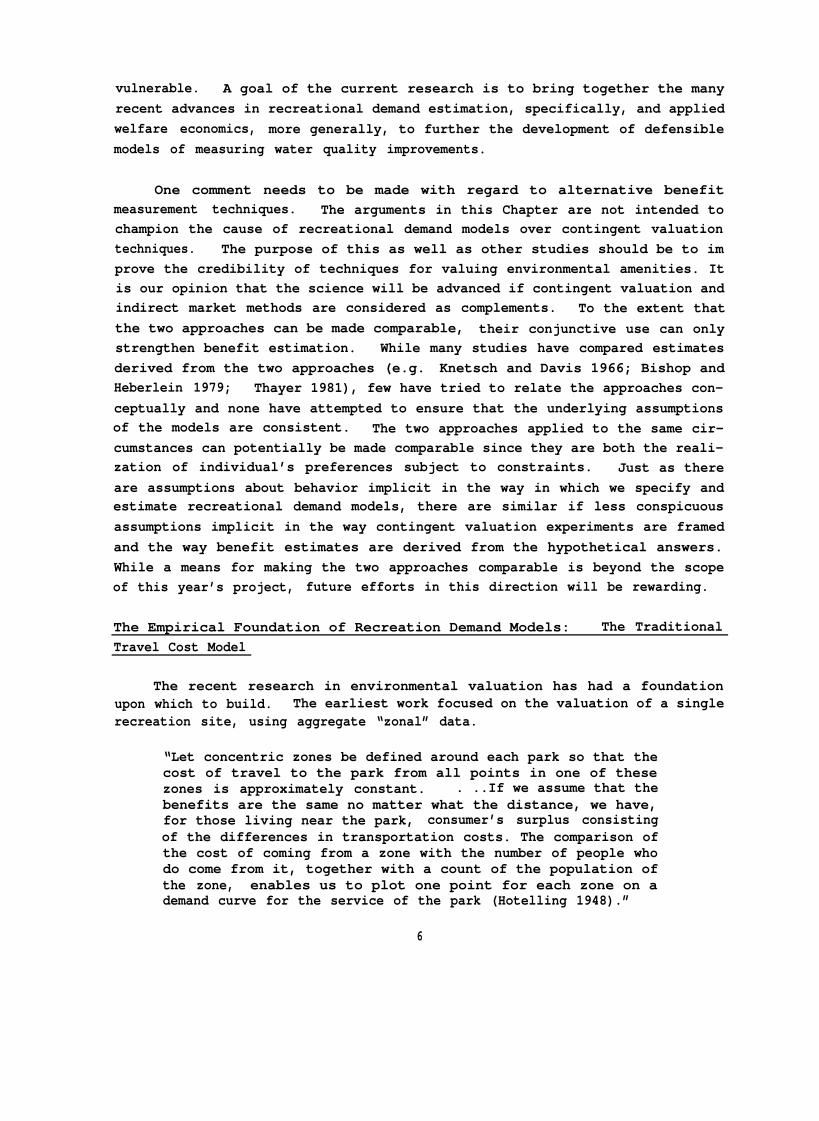
The recent research in environmental valuation has had a foundationupon which to build. The earliest work focused on the valuation of a singlerecreation site, using aggregate “zonal” data.
“Let concentric zones be defined around each park so that thecost of travel to the park from all points in one of thesezones is approximately constant. . ..If we assume that thebenefits are the same no matter what the distance, we have,for those living near the park, consumer’s surplus consistingof the differences in transportation costs. The comparison ofthe cost of coming from a zone with the number of people whodo come from it, together with a count of the population ofthe zone, enables us to plot one point for each zone on ademand curve for the service of the park (Hotelling 1948).”
6
In fact the development of methods of estimating the demand for recreationso closely paralleled the use of zonal models that the so-called travel costmethod is often considered synonymous with the use of zones.
The concept of this original travel cost model took advantage of thefact that unlike other goods, recreational sites are immobile and users mustincur specific costs to access a site. Thus, travel costs were proposed asa proxy for market price, with consumption of the recreational opportunityexpected to decline as distance from the site and travel costs rose.Clawson, in 1959, and Clawson and Knetsch, in 1966, developed the travelcost idea into an operational model by estimating demand for a recreationsite and measuring the total value or benefits of the site.
This basic model has been widely replicated and extended to account forvarious complexities of the recreation experience. The procedure is recom-mended for project benefit estimation in the 1979 revision of the WaterResources Council’s “Principles and Standards.” Thus a long evolutionaryprocess has established a precedent for the use of travel cost models invaluing aspects of recreation activities.
The essence of the traditional travel cost approach to valuing benefitsis shown in Figure 1.1. The sum of travel costs and entrance fees act as asurrogate for the price of the recreational trip. The demand curve of a“representative” individual is estimated by regressing trips per capita ineach zone against average travel cost per trip and other average charac-teristics of each zone. An aggregate demand curve is then formed by com-bining the representative demand curve with zonal characteristics of thepopulation. The shaded area between the aggregate demand curve and theactual entrance fee is viewed as a measure of the consumers’ surplus fromthe site.
Price(travel cost &entrance fee)
Recreation trips/time period
Figure 1.1: The Recreation Demand Curve
7
The fundamental problem with using the simple travel cost approach asshown above is that it is defensible only in certain rather restrictivecircumstances. Much of the research since 1970 has expanded the travel costmodel to a more general recreational demand model, making it more defensiblein a wider variety ofbenefit estimation, ahas been established.techniques is present
circumstances. In addition, because its role has beencloser correspondence to axioms of welfare economicsDevelopment of increasingly sophisticated estimation
throughout this period.
The Theoretical Foundation of Recreation Demand Models: The HouseholdProduction Approach
While the travel cost method has been applied to empirical problems fordecades, its connections with the theory of welfare economics have onlyrecently been articulated. With the increased acceptance of benefitmeasurement by the economics discipline in the 1970’s came the need to linktravel cost valuations to welfare theory. The travel cost method had restedmainly on the presumed analogy between travel costs and market prices. Inthe 1970’s more general models of individual behavior, such as the householdproduction function, established the link between travel cost and individualutility maximizing behavior giving greater credibility to existing empiricalpractices.
The household production framework is not an approach to estimation buta general model of individual decision making. Its antecedent can be foundin the economics literature on the allocation of household time among marketand nonmarket employment (Becker, 1965; Becker and Lewis, 1973).placability of the household production framework for recreationwas first noted by Deyak and Smith (1978) and later exploredCharbonneau and Hay, (1978).
The household production function takes a broader view ofconsumption than traditional market approaches. Commodities,
The ap-decisionsby Brown,
householdfor which
individuals possess preferences and from which they derive utility, may notbe directly purchasable in the marketplace. In fact some goods which can bepurchased may not yield utility directly but may need to be combined withother purchased goods and time to generate utility. Rarely are goods com-bined by the household rather than by firms unless they require substantialtime inputs. Thus, time is a critical feature of the model.
One can then view the household as a producer, purchasing inputs, sup-plying labor, and producing commodities which it then consumes. This makesfor a perfectly defensible utility theoretic decision model which can beexpressed as
(lb)
(lc)
(1d)
where z’s are commodities, x’s are market goods, and p their prices, tx istime spent producing commodities, tw is time spent working, w is the wagerate, Y is wage income, R is nonwage income, and T is total time endow-ment. Included in the above series of expressions is the usual utilityfunction (la), a budget constraint (lc), a production function for the z’s(lb), and a time constraint (1d). If one of the z’s represents recreationaltrips with inputs of time, transportation, lodging, equipment, etc., then wehave the makings of a recreational demand model.
Acationway inments.
major contribution of this framework is that it provides a justifi-for using the travel cost model in certain instances, as well as awhich to generalize the traditional model to incorporate other ele-While the household production framework provides a general and
flexible way of presenting the individual’s (household’s) decision problem,restrictions are required to make the model empirically tractable. Onedifficulty inherent in the general form is that the marginal cost of pro-ducing a zi is likely to be nonlinear. The implications of this forestimation and welfare evaluation are explored in Bockstael and McConnell(1981, 1983) and an application can be found in Strong (1983). If the pro-duction technology is Leontief and there is no joint production, however,the marginal cost of producing a z1 (e.g. a recreation trip) is constant andthus functionally analogous to a market price.principal input and ignoring the time dimension equates this model to thetraditional travel cost model. Travel costs no longer depend for theircredibility on being a “proxy” for market price. They are a legitimatecomponent of the marginal cost of producing a trip.
It is important to note that this model, as well as all of welfaretheory, is grounded in individual behavior. For this reason, and other morepractical ones, researchers have tended to move toward using individualobservations rather than zonal averages in more recent applications. Thezonal-individual observation controversy will receive greater attention inChapter 3.
The general model also offers a framework from which other aspects ofrecreational demand, such as the opportunity cost of time, can be introduced(Desvousges, Smith and McGivney, 1983). As far back as Clawson, research-er’s knew time costs were an important determinant of recreational demand.However, these costs have often been ignored or treated in an ad hocfashion. A treatment of time, which is theoretically consistent and empiri~cal tractable, is the subject of Chapter 4.
The Plan of Research for Part I
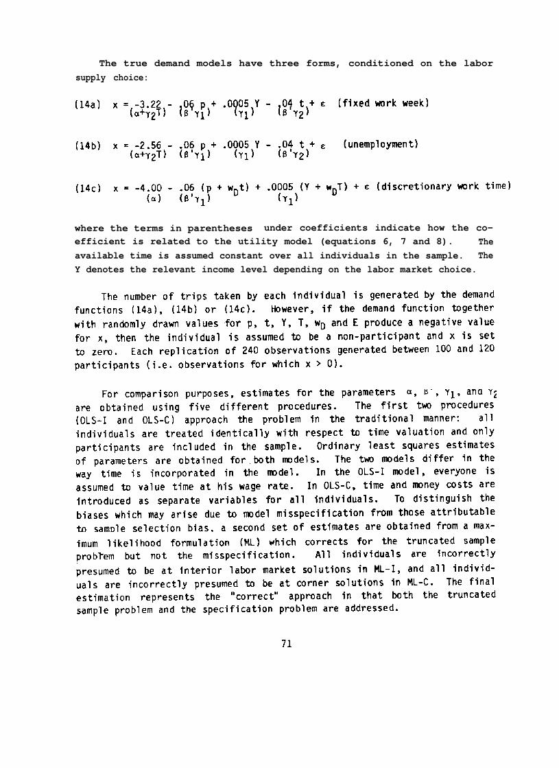
The conceptual problems which are addressed in Part I have been chosenbecause benefit estimates have turned out to be extremely sensitive to theirarbitrary treatment. In each case attempts have been made to show the sen-sitivity by citation to existing literature, by use of existing data sets,or by simulating behavioral experiments. Also we demonstrate, by usingexisting data or simulation results, the application of each improvementwhich we develop.
Two criteria are used in the development of improved techniques: theo-retical acceptability and empirical tractability. Improvements are proposedonly if they can be implemented with accessible econometric techniques andwith data which can reasonably be collected with manageable surveys.
Part I makes substantive contributions to the single site or activityrecreation demand model. Several issues - such as the treatment of time,specification and functional form, aggregation and benefit estimation - areexplored. This work forms the foundation for the multiple site modellingtechniques discussed in Part II.
10
CHAPTER 2
SPECIFICATION OF THE RECREATIONAL DEMAND MODEL:FUNCTIONAL FORM AND WELFARE EVALUATION
In the period of only a few years, a number of theoretical papersconcerning precision in welfare measurement and the relationship among wel-fare measures has emerged. Perhaps the most often cited of these is byWillig (1976), who has shown that the differences among ordinary consumersurplus, compensating variation, and equivalent variation are within boundswhich are determined by the income elasticity of demand and the ratio ofordinary surplus to total income. The issue of the accuracy of the approxi-mation has become less consequential since the work by Hanemann (1979,1980b, 1982d), by Hausman (1981), and by Vartia (1983). The first two haveshown how to recover exact welfare measures from some common functionalforms of demand functions. The latter has developed algorithms yieldingnumerical solutions which provide arbitrarily close approximations to truewelfare measures for functional forms which have no closed form solutions.The first part of this chapter provides a review of this literature on inte-grability and exact welfare measures.
The second part of the chapter addresses the choice of functionalform. While a particular functional form may be consistent with some under-lying preference function, it may not be a preference structure consistentwith actual behavior. That is, arbitrary choice of functional form mayimply too specific a preference structure and one which is inappropriate forthe sample of individuals.
The sensitivity of benefit estimates to functional form has frequentlybeen cited in the literature and may be far greater than differences betweenHicksian variation and ordinary surplus measures of benefits. This chaptersuggests one means of addressing the choice of functional form. We show howclose approximations to compensated welfare measures can be derived fromflexible forms of the demand function. Emphasis is given to the choice offunctional forms which are both consistent with utility theory and supportedby the data.
11
The Intergrability Problem and Demand Function Estimation
There are two general ways to develop utility theoretic measures ofconsumer benefits. The first employs an assumed utility function from whichdemand functions are derived through the appropriate constrained utilitymaximization process. The other begins with a demand specification andintegrates back to a utility function.
The preferable approach depends on whether the problem in questioninvolves a single good or a vector of related goods. In general, it isdesirable to begin with a demand function and integrate to derive welfaremeasures. As Hausman points out, the only observable information is thequantity-price data, data which can be used to fit demand curves not utilityfunctions. Good econometric practice would suggest we choose the bestfitting form of the demand function among theoretically acceptable candi-dates. The demand function approach is preferable because it allows theresearcher to include as choice criteria how closely the functional formcorresponds to observed behavior. For these reasons this approach will beused for single site models. Unfortunately, multiple good models posesevere integrability problems. As such we are forced in the latter half ofthis volume to employ the alternative approach of first choosing a prefer-ence structure and then deriving demand functions from that structure.
The conditions for integrating back to an indirect utility functionfrom demand functions are now well known. Integrability depends on solvingthe system of partial differential equations:
(1)
where m is income, p is the price vector, and xi and pi are the quantityThe solution is called the income
compensation function m(p,c), where c is the constant of integration. This
function is identical to our concept of the expenditure function, if c istaken as an index of utility.by inverting m(p,u) to obtain U=V(p,m). Hurwicztial differential equations of the type in (1)xi(.) are single valued, differentiable functsymmetry conditions hold:
ty function can be derived(1971) has shown that par-have solutions if a) theons and b) the Slutsky
If the problem of interest involves just one good, the convention is toassume that the prices of all other goods (those not of immediate interest)either are constant or move together so that these goods can be treated as aHicksian composite commodity with a single price. This price can be repre-sented by a price index, or set to one when price is unlikely to vary overthe sample. The problem is now reduced to the two good case: x and a com-posite commodity. Since a system of N partial differential equations canalways be replaced by a system of N - 1 such equations by normalizing onthe price of one good, the two good case requires the solution of only onedifferential equation. There is only one element to the Slutsky matrix now,so there is no question of symmetry, and any function which meets regularityconditions is mathematically integrable (although a closed form solution forthe expenditure function may not always exist).
Mathematical integrability does not necessarily imply economic inte-grability, i.e. that the implied utility function be quasi-concave.Economic integrability conditions require that a) the adding-up restrictionshold, i.e. p’x=m, and the functions are homogeneous of degree zero inprices and income and b) the Slutsky matrix is negative semi-definite, i.e.
Hanemann (1982d) has shown that for the two good case the adding-up propertyimplies the homogeneity property, so that for this case one need only checkthat the negative semi-definite condition holds. However, this lattercondition is nontrivial; its violation may cause anomolies to arise in thecalculation of welfare measures. Violation of negative semi-definitenessconditions implies upward sloping compensated demand functions and meaning-less welfare measures.
Exact Surplus Measures for Common Functional Forms
Closed form solutions to (1) are possible for several commonly usedfunctional forms. The procedure discussed above and outlined in theAppendix 2.1 to this chapter has been used to derive parametric bivariateutility models consistent with tractable ordinary demand functions. In whatfollows, the results of this procedure when applied to the linear, semi-log,and log-linear demand functions are presented (for reference see Hanemann,1979, 1980b, 1982b; Hausman 1981).
13
and
where U'and mo.i.e. the
Not
CV =
EV =
takes the value of the indirect utility function evaluated at p'The expressions for CV and EV as well as that for ordinary surplus,Marshallian consumer surplus, are also recorded in Table 2.1.
all estimated demand functions corresponding to the functionalforms in (2), (3) and (4) can be integrated back to well behaved (i.e.quasi-concave) utility functions. The negative semi-definiteness condition
14
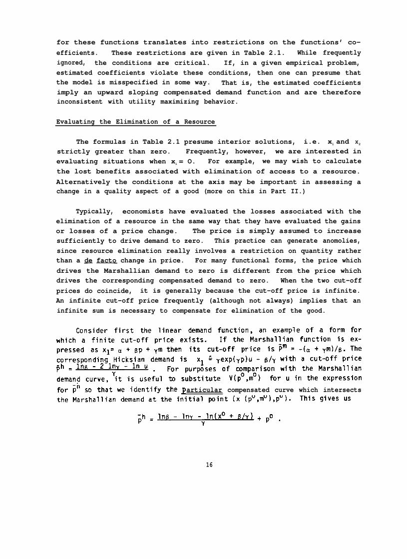
for these functions translates into restrictions on the functions’ co-efficients. These restrictions are given in Table 2.1. While frequentlyignored, the conditions are critical. If, in a given empirical problem,estimated coefficients violate these conditions, then one can presume thatthe model is misspecified in some way. That is, the estimated coefficientsimply an upward sloping compensated demand function and are thereforeinconsistent with utility maximizing behavior.
Evaluating the Elimination of a Resource
The formulas in Table 2.1 presume interior solutions, i.e. xl and X2
strictly greater than zero. Frequently, however, we are interested inevaluating situations when xl = O. For example, we may wish to calculatethe lost benefits associated with elimination of access to a resource.Alternatively the conditions at the axis may be important in assessing achange in a quality aspect of a good (more on this in Part II.)
Typically, economists have evaluated the losses associated with theelimination of a resource in the same way that they have evaluated the gainsor losses of a price change. The price is simply assumed to increasesufficiently to drive demand to zero. This practice can generate anomolies,since resource elimination really involves a restriction on quantity ratherthan a de facto change in price. For many functional forms, the price which— —drives the Marshallian demand to zero is different from the price whichdrives the corresponding compensated demand to zero. When the two cut-offprices do coincide, it is generally because the cut-off price is infinite.An infinite cut-off price frequently (although not always) implies that aninfinite sum is necessary to compensate for elimination of the good.
articular compensated curve which intersects
16
Because the bounds of integration for CV are not the same as for OS andEV, the usual relationship between the latter and former is destroyed andWillig’s bounds no longer hold. Whether or not the difference is ofpractical significance depends on the relative sizes of the parameters andcan only be determined empirically. Unfortunately the greater the differ-ence between ordinary surplus and compensating variation, the greater thedifference in the two CV measures.
17
To understand this phenomena, one needs to consider the concept ofessentiality. Marty equivalent definitions of essentiality exist but perhapsthe most intuitive and descriptive is the following:
is essential if, given an initial consumption
An equivalent definition is that there exists no finite sum which can com-These definitions are both equivalent to
the condition that for xl to be essential
and for xl to be nonessential
It should be noted that these definitions are in terms of the compensatednot the ordinary demand function. In fact, there is not a perfect corres-pondence between the limiting conditions for the compensated demands andthose for the ordinary demands. There exist preference structures whichimply ordinary demand functions which do converge but compensated functionswhich do not.
general CES form for thegenerates the following
functions:
18
19
Functional Form Comparison
While there are no previous studies where compensating variationmeasures are compared across functional form, there are some which documentthe potential differences in ordinary surplus estimates which arise whendifferent functional forms are estimated on the same data and others whichsimply address the issue of choice among functional form in recreational de-mand models. In a study of warm water fishing in Georgia, Ziemer, Musserand Hill (1980) assessed the importance of the functional form on the sizeof ordinary consumer surplus estimates. They chose to consider linear,semi-log and quadratic forms and found average surplus per trip estimates of$80, $26 and $20 respectively. The researchers estimated a BOX-COX trans-formation to discriminate among the three functional forms and determinedthat the semi-log was preferable.3
Two other papers of note identified the semi-log function as most ap-propriate. Both papers addressed functional form in the context of theheteroskedasticity issue (a more detailed discussion of these papers can befound in Chapter 3). Vaughan, Russell and Hazilla (1982) tested for appro-priate functional form and heteroskedasticity, simultaneously. They usedthe Lahiri-Egy estimator which is based on the Box-Cox transformation, butalso incorporates a test for nonconstant variance. They concluded thatboth the linear heteroskedastic and linear homoskedastic models were inap-propriate. The semi-log form which did not exhibit heteroskedasticity wasfound to be preferable. In a second paper Strong (1983a) compared the semi-log model with the linear model based on the mean squared error in predict-ing trips. She also found that the semi-log function performed better.
To try to establish more conclusively which functional form was moreappropriate, Smith chose to use a method suggested by Pearsan which discrim-inates between non-nested competing regression models. Smith found that inhis sample of wilderness recreators he was able to reject both the semi-logand the double-log functional forms based on this criteria. His conclusion
20
that the travel cost model may be inappropriate for wilderness recreationmodelling may be correct but is too extreme a conclusion to be supported bythis analysis. Even if the Desolation Wilderness area is representative ofother wilderness recreation problems, the alternatives tested in this studyare by no means exhaustive. The functional forms chosen are but three amonga vast array of choices. Additionally, Smith’s poor statistical resultscould well be a reflection of other specification problems inherent in hisconventionally designed zonal travel cost model. (See discussions inChapters 3 and 4.)
Estimating a Flexible Form and Calculating Exact Welfare Measures
Each of the above studies was concerned with calculating ordinarysurplus measures from commonly estimated functional forms using zonaldata. These studies either implicitly assumed or explicitly demonstratedthat consumer surplus estimates would differ depending on the choice offunctional form. Not surprisingly, compensating (or equivalent) variationmeasures derived from different functional forms may also exhibit vastdifferences.
In the previous literature, the focus seems to have been one ofidentifying a means of choosing which of the popular functional forms waspreferable. If it were possible to select one, then the exact welfareresults of the previous section could be directly applied. Many of thearticles appear to point to the semi-log as a desirable form, yet theevidence is far from conclusive and there is no reason to believe that thesame form would necessarily be appropriate for all situations.
It would be far preferable to consider a wider array of functionalforms than the three discussed above and to allow the data to choose amongthem. One way to access a slightly broader range of functional forms is toestimate a flexible form such as the BOX-COX transformation. However, Box-Cox forms do not in general integrate back to closed form expressions forthe expenditure or indirect utility functions. A solution to this problemcan be found in the recent work by Vartia (1983), among others, who demon-strates a means of obtaining extremely close approximations to compensatingvariation when exact measures are not possible. The procedure uses a thirdorder numerical integration technique to obtain an approximate solution tothe differential equation.
21
The Vartia algorithm,appealing proposition. Theclose in the neighborhoodcurves which occurs with aadjustment in consumption
and others like it, is based on an intuitivelyordinary and compensated demand curves are veryof their intersection. The difference in themovement away from that intersection reflects anin response to additional (compensations in)
rounding error will eventually take their toll.
As pointed out above, the difficult tasklation of the appropriate income compensation
into
the procedure is the calcu-accompany each price step.
thenois
half of one percent of the true measure. Thusto meet an acceptable tolerance criteria at low
In what follows, we will demonstrate howcan be used with the BOX-COX transformation.
the approximation would seemcomputing costs.
this approximation procedureThe approach is equally ap-
plicable to other forms (flexible or not) for a single equation or system ofequations. It should be noted, however, that the Vartia approximation doesnot circumvent either mathematical or economic integrability conditions.These conditions must hold for the results of the procedure to have mean-ing. The Vartia technique provides aand equivalent variation measures whenferential equation in (1) exists or can
An Illustration
To illustratecalculating welfaresportfishing data.
the application of this
close approximation to compensatingno closed form solution to the dif-easily be found.
method for choosing functional form andmeasures, the BOX-COX transformation was estimated for a set ofThe BOX-COX approach was chosen because of its wide familiarity
and ease of estimation. However, as noted above, the procedure for deriving welfaremeasures is equally applicable to other less restrictive functional forms.
All individuals in the group took at least one trip of greater than 24hours on a party/charter boat. This is a subset of a sample of 1383 sport-fishermen who responded to a mail questionnaire asking details of their 1983sportfishing activities in Southern California. A complete description ofthe data can be found in National Coalition for Marine Conservation (1985).
For purposes here, an individual’s demand for party/charter trips (x)is considered to be a function of costs of the trip (c), income (y) andcatch of target species (b).
Three models were estimated using the same data set. The first con-strained the functional form to be linear, the second employed a semi-logfunction and the third used the more flexible BOX-COX transformation on the
.A
where x is trips and z is the vector ofeters to be estimated included the usualBOX-COX parameter, y .
took the form:
variables. The param-
24
In Table 2.2, the results of this experiment are presented. The esti-mated coefficients from the linear and semi-log models have been used inconjunction with the expressions in Table 2.1 to calculate estimates ofordinary surplus, and compensating and equivalent variation. The compu-tation process is explained in Appendix 2.1. The Vartia algorithm has beenused to obtain “approximate” measures of compensating and equivalent varia-tion and ordinary surplus for the BOX-COX model. The algorithm is presentedin Appendix 2.2.
Some important points are worth noting. First, these welfare measuresseem large. It should be remembered that the sample included only those whotook longer thanindividuals. Inally, there arecoefficients mayerations will be
one day trips and are therefore likely to be rather wealthyfact, the mean income of this group is $58,000. Addition-reasons why welfare measures calculated from estimatedproduce overestimates of the true values. These consid-discussed in Chapter 5.
25
The important point for consideration here is that if one were arbi-trarily to choose between the linear and semi-log specification inestimating the demand function, widely divergent benefit estimates wouldemerge. In the case above there is only a 3 to 5% difference across welfaremeasures (CV, EV, 0S) for any one functional form, but a 16 to 19% differ-ence between the two most commonly used functional forms. The BOX-COXtransformation offers a means of choosing among a continuous range offunctional forms. In the example above, it seems to support the semi-logfunction. In other cases we have tried, where neither the linear nor thesemi-log results appear superior, the BOX-COX analysis often selects an isignificantly different from either zero or one. Then the Varita routine isnecessary to calculate compensating and equivalent variation approximations.
While definitional differences in welfare measures will be of greaterconcern in problems with larger income elasticities (Willig, 1976), boundson these differences are well developed, at least for simple models. Thepotential differences from functional form, however, may not be so wellappreciated.
Table 2.2
Welfare Estimates
Calculated from Different Functional Forms
(annual average estimates for a sample of Southern California sportfishermen)
Functional Form
CompensatingVariation
OrdinarySurplus
EquivalentVariation
8339
8042
7899
6999
6877
6763
Linear Box-Cox Semi-log
6950
6812
6779
26
FOOTNOTES TO CHAPTER 2
1 LaFrance and Hanemann (1985) describe the process of obtaining directutility functions from estimated demand functions for systems of demandequations.
2 There is some disagreement in the literature as to the precise form ofthe compensating and equivalent variation expression. All agree thatcompensating and equivalent variation must be of the same sign. How-ever, differences of opinion exist as to whether the variationalmeasures have the same or the opposite sign as the utility change.Here we adhere to the convention used by Just, Hueth and Schmitz (1982)which seems most closely aligned with the original description ofHicks. Compensating and equivalent variation are positive (negative)for price changes which generate increases (decreases) in utility.
Box Cox models are estimated by maximizing the maximum liklihood
4 The Lahiri-Egy estimation is an extension of the BOX-COX transfor-mation. It introduces an additional parameter which allows one to testfor the presence of heteroskedasticity jointly with functional form.The estimator assumes that the error in the model
28
APPENDIX 2.1
DERIVATION OF SOME UTILITY THEORETICDEMAND SYSTEMS
MEASURES FROM TWO GOOD
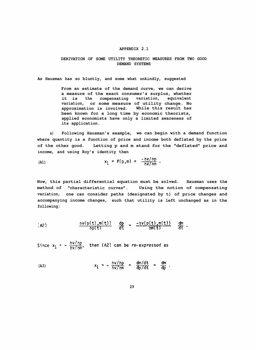
As Hausman has so bluntly, and some what unkindly, suggested
From an estimate of the demand curve, we can derivea measure of the exact consumer’s surplus, whetherit is the compensating variation, equivalentvariation, or some measure of utility change. Noapproximation is involved. While this result hasbeen known for a long time by economic theorists,applied economists have only a limited awareness ofits application.
a) Following Hausman’s example, we can begin with a demand functionwhere quantity is a function of price and income both deflated by the priceof the other good. Letting p and m stand for the “deflated” price andincome, and using Roy’s identity then
(A1)
Now, this partial differential equation must be solved. Hausman uses themethod of “characteristic curves”. Using the notion of compensatingvariation, one can consider paths (designated by t) of price changes andaccompanying income changes, such that utility is left unchanged as in thefollowing:
(A3)
29
This gives an ordinary differential equation which in many cases can besolved with fairly standard techniques. As Hausman shows, the solution tothe differential equation
The only confusion is in dealing with, c, the constant of integration.Clearly c will not be a function of any of the parameters in the demandfunction but it will certainly be a function of the utility level. In asense it doesn’t matter what function as long as it is increasing andmonotonic, since we have no way of measuring or interpreting absolute levelsof utility. As a consequence Hausman simply substitutes Uo for c which is
try to interpret In some circumstances
appear to be negative. There is no fundamental problem, however, as long as
b) Once the expenditure function is obtained from solving the differ-ential equations the indirect utility function is usually easy to obtain by
For some demand functions,it is easier to integrate back to the indirect utility function first, in
as a function of utility and price. The three examples below demonstratehow straightforward this can be when there are closed form expressions forboth indirect utility and expenditure functions:
(log-linear)
c) Once the expenditure function is derived, the Hicksian demandfunction together with compensating and equivalent variation measures are ofcourse quite accessible:
30
An example is presented for the linear demand, where
d)function,properties
which is of interest because it best portrays theof the preference function being assumed. The task is to convert
a utility function in (normalized price) and income into a utility functionSince we have two functions which relate the x’s
with p and m, i.e. the Marshallian demand function for xl and the budgetconstraint, it is conceptually possible to make the transformation. One
and then the substitution into the indirect utility function isstraightforward.
As an example, consider the linear case where
xl
m
then
By substitution
32
APPENDIX 2.2
COMPUTER ALGORITHM FOR OBTAINING COMPENSATING ANDEQUIVALENT VARIATION MEASURES FROM ESTIMATEO
-5, B2=6, THEN THE FOLLOWING SHOULD BE ENTERED* 10 X1(P1,INCOME)=2-5*P1+6*INCOME* A SYSTEM OF UP TO 20 EQUATIONS CAN BE ENTERED IN THIS WAY. THE FUNCTION* CALLS THROUGHOUT THE PROGRAM MUST BE MODIFIED TO REFLECT THE APPROPRIATE* ARGUMENT LIST FOR THE FUNCTIONS BEING USED. THE # OF EQUATIONS AND THE* # OF STEPS FOR THE PRICE PATH MUST BE SUPPLIED. AVOID A LARGE # OF STEPS+ (>500) AS ROUNDING ERRORS CAN BECOME SERIOUS.+ SAMPLE PROGRAM BELOW DEMONSTRATES TWO GOOD, ONE PRICE CHANGE CASE.* * * * * * * * * * * * * * * * * * * * * * * * * * * * * * * * * * * * * * * * * * * * * * * * * * * * * * * * * * * * * * * * * * * * * * * * * * * * * * +
EPS=0.000I**********ii********* PROBLEM SIZE *******************
WRITE (6,1)
* This algorithm was developed by Terrence P. Smith, Department ofAgricultural and Resource Economics, University of Maryland, CollegePark, Maryland.
33
1 FORMAT (’ ENTER THE # OF EQUATIONS IN THE SYSTEM’,/,AND THE # OF STEPS FOR THE PRICE PATH’)
READ (5,*) NEQ,NWRITE (6,2)
2 FORMAT (’ SPECIFY THE INITIAL AND FINAL VALUES FOR EACH’,/,* ‘ PRICE, IN ORDER. IF A PRICE DOESNT CHANGE, SPECIFY’,/,* ‘ SAME INITIAL AND FINAL PRICE.’)READ (5,*) ((P(I,1),P(I,N)),I=1NEQ)WRITE (6,3) ((I,P(I,1),P(I,N)),I=1NEQ)
3 FORMAT (’ INITIAL PRICE FINAL PRICE ‘,/,20(1H,I2,2F10.4,/))WRITE (6,4)
4 FORMAT (’ NOW ENTER THE INCONE LEVEL’)READ (5,*) YO
******************** CALCULATE THE PRICE STEPS AND PATHS ***********
DO 1000 I=1,NEQPSTEP(I)=(P(I,N)-P(I,1)/NDO 1000 J=2,N-1P(I,J)=P(I,J-1)+PSTEP(I)
1000 CONTINUE******************** CALCULATE THE INITIAL VALUES
2000 CONTINUE******************** ALGORITHM
* ETC.TERM(I)=((XT(I)+XC(I))/2)*PSTEP(I)
************
***********
4000 SUM=SUM+TERM(I)NEWY=SUM+YOSUM=OY=NEWYIF (ITIMES.EQ.500) STOP ‘ENDLESS LOOP - NOT CONVERGING’
DO 5000 I=I,NEQ5000 XC(I)=XT(I)
IF (DABS(NEWY-OLDY).GT.EPS) GO TO 500ITIMES=OYO=NEWY
5 FORMAT (IHO, ‘COMPENSATED DEMANDS’, 13X, ’COMPENSATED INCOME’)
6 FORMAT (1H ,5X,FIO.4,17X,F1O.4)STOPEND
34
CHAPTER 3
AGGREGATION ISSUES:THE CHOICE AMONG ESTIMATION APPROACHES*
Our ultimate use of the recreational demand model is to deriveaggregate welfare measures of the effects of environmental changes. How-ever, the means by which these aggregate measures should be devised dependsupon the level of aggregation of observations and the treatment of users andnonusers in the estimation stage. Thus , the appropriate aggregation ofwelfare measures depends very much on the initial decisions as to the typesof observations used and the general sampling strategy employed.
Problems of aggregation plague applications of macroeconomics. Thetheory is derived from postulates of individual behavior, yet data is oftenmore readily accessible in an aggregate form. In many types of micro-economic problems, market data is so much easier to obtain that rarely arecross sectional, panel data used. However, in recreational demand studies,where markets do not usually exist, survey techniques are necessary to gen-erate data. Even in such surveys, however, data are often collected inaggregated form (by zone of residence). To many, the travel cost method is,in fact, synonymous with the “zonal approach”, which employs visit rates perzone of origin as the dependent variable and values for explanatory vari-ables which represent averages for each zone.
In its current state, the travel cost approach to valuing nonmarketbenefits is the product of two legacies. One dates back to HaroldHotelling’s extraordinary suggestion for estimating recreational demand. Ithas become intimately linked to the zonal approach and dependent on theconcept of average behavior. The other legacy is the axioms of appliedwelfare economics which provide defensible means of developing benefit
* This Chapter is the work of Kenneth E. McConnell, Agricultural andResource Economics Development, U. of Maryland, and Catherine Kling,Economics, U. of Maryland.
35
measures based on individual behavior. The two comeissue which we broadly define as aggregation.
This chapter explores the relationship betweenapproach and a model based on individual behavior. Adiscussion is the treatment of both recreational parti
in conflict over this
the traditional zonalcentral theme in thiscipants and nonpartic-
ipants. The implications for estimation and benefit calculations arediscussed.
A Review of Past Literature
Before addressing the issues anew, it is useful to put in perspectivethe various discussions of aggregation problems found in the existing liter-ature. The term “aggregation” has been“national benefits” literature. Thesewidespread improvements in water qualitymental regulations. In this literature,estimating benefits over a vast numbergeographical regions, and recreational
applied in what we shall call thetypes of studies attempt to valuedue to changes in national environ-the “aggregation problem” involvesof widely divergent water bodies,users. Vaughan and Russell have
developed methods to evaluate comprehensive policy changes in this context(see, for example, Vaughan and Russell, 1981 and 1982; Russell and Vaughan,1982 ) ● Perfecting these methods for obtaining approximate “value per userday” figures is of considerable importance and is being pursued underanother EPA Cooperative Agreement.
The research reported here, however, is not designed to address theseissues. The aggregation issues in question in this study are those whicharise in all studies which attempt to use travel cost (or its more generalform - household production) models to evaluate benefits to all individualsaffected by an environmental change. The following brief review offers amenu of the problems which have been raised concerning aggregation withinthe context of the zonal and individual observation approaches to the travelcost method.
1. The Zonal ApproachTravel cost models that employ the zonal approach generally regress
visits per capita in each zone of residence on the travel cost from theassociated zone to the resource site and on other explanatory variables.The literature on these zonal models has addressed two types of problems.The appropriate size and definition of the zones and heteroskedasticityproblems in estimation.
36
Sutherlandaffected demanduse concentric
(1982b) questioned the degree to which the size of the zonesand benefit estimates and whether it was more appropriate tozones or population
for boating using ten and twentytwenty population centroids. Theestimates when concentric zonescentroids, suggesting that benefitmodel will be sensitive to the
centroids. He estimated demand curvesmile wide concentric zones as well asstudy revealed larger consumer surpluswere used as compared to populationestimates obtained from a travel costzone definition. However, Sutherland
lamented the absence of clear criteria for choosing either populationcentroids or concentric zones.
In a recent paper, Wetzstein and McNeely (1980) discussed a relatedissue of aggregating observations. They argued that if it is indeed neces-sary to use aggregate data (i.e. zonal rather than individual observations),it is more efficient to aggregate the observations by similar travel costsrather than by the more traditional method of similar travel distances todetermine zones. Aggregating the zones by travel cost would provide “a moreefficient estimate of the coefficient associated with cost and thus improvethe confidence in the value of the coefficient” (p. 798).
Wetzstein and McNeely estimated demand equations for ski areas underthe two alternative aggregation schemes. When the data were aggregated bycosts, both the distance and cost coefficients were significantly differentfrom zero. However when the data were aggregated by distance, only thedistance coefficient was significant. The paper suggests that estimatedcoefficients, and thus benefit estimates, may be highly sensitive to varia-tion in explanatory variables within zones.
The final issue that has arisen concerning thehas to do with the spatial limits of the travel cost(1980) pointed out that including zones far from thelikely violate some basic assumptions implicit in thethe distance between origin zone and site increases,
determination of zonesmodel . Smith and Koppsite being valued willtravel cost model. Asit is less likely that
the primary purpose of the trip is to visit the site in question. It isalso less likely that the amount of time spent on site and the form oftransportation will remain constant. Smith and Kopp proposed the use of astatistical test to determine which zones should be included in the modeland which should not. This test was developed by Brown, Durbin and Evans(1975) and is based on the fact that observations inconsistent with theassumptions of the travel cost model will produce nonrandom errors.
37
Smith and Kopp used 1972 United States Forest Service data on visitorsto the Ventana area to illustrate the impact that the spatial limits of thetravel cost model can have on benefit estimates. They had information onvisitors from 100 zones encompassing 38 states. Applications of the Brown,Durbin and Evans procedure suggested that a spatial limit to the model couldbe established at a distance of about 675 miles from the site. The esti-mated per trip consumer surplus lost if the area were destroyed was $14.80when all observations were included, but only $5.28 when the apparentspatial limits of the model were respected. Thus the definition of zonesand the limitation of the number of zones are important issues and can havea significant impact on the size of benefit measures.
Another issue that has arisen in applying the zonal travel cost modelconcerns possible heteroskedasticity in the error term. This issue has beenintegrally related to the assumed functional form of the demand equation.Bowes and Loomis (1980) were among the first to warn of the potentialheteroskedasticity problem which zonal data may create. When the definedzones encompass different size populations, the variance of the dependentvariable, average number of trips in each zone, will vary with zones. Ifthe variance of each individual’s visitation rate is the same, i.e.
mean visits per capita from zone j wI1l be
Nj is zone j’s population. This is a classic heterosskedasticity problem forwhich the correction procedures are well understood. One simply needs toweight all variables by the square root of the zone’s population.
To illustrate the potential importance of this correction, Bowes andLoomis estimated a linear demand equation for per capita trips down asection of the Colorado River in Utah. Using the unweighed OLS estimates,total benefits were calculated as $77,728. When weighted observations wereused to correct for the apparent heteroskedasticlty, only $24,073 inbenefits could be attributed to the users of the Westwater Canyon.
Another possible source of nonconstant variance is suggested byChristianson and Price (1982). They argue that the variance in individualvisitation rates is not likely to be constant across zones. Individualslocated at different distances from the site will exhibit different partici-pation rates and can be expected to have different individual variances.The source of heteroskedasticity is the unequal visit rates across zones. Ifboth types of heteroskedasticity exist, the authors suggest that the properweighting scheme would be
38
is mean visitation rate per capita in zone j. This pro-cedure causes the dependent variable to appear on the right hand side of theequation and thus would seem to generate further statistical problems.
In her response to Bowes and Loomis, Strong (1983b) made the case forthe use of a nonlinear function (specifically the semilog form) as an alter-native to the Bowes and Loomis correction for heteroskedasticity. Linearand semilog demand equations for steelhead fishing were estimated using datafrom zones around twenty-one rivers in Oregon, and a Goldfeld-Quandt testwas employed to test for the existence and size of heteroskedasticity. Thesemilog model did not require a heteroskedasticity correction, but thelinear model did. After correcting the linear model for heteroskedasticity(applying the appropriate weights), this model was compared to the semilogmodel by the mean squared error in predicting trips. The semilog form per-formed better than the corrected linear model in this test.
Vaughan, Russell and Hazilla (1982), in another comment on the Bowesand Loomis article, argued that an alternative to assuming a linear demandequation and heteroskedasticity is to test for both in the data rather thanimpose them as assumptions. To do this, they tested the Bowes and Loomisdata for appropriate functional form and heteroskedasticity simultaneouslyby applying the Lahiri-Egy estimator which utilizes a maximum likelihoodprocedure to estimate the appropriate functional form with a BOX-COX trans-formation under conditions of potential heteroskedasticity. As a result ofthis procedure, they were able to reject the linear homoskedastic and thelinear heteroskedastic models. The appropriate functional form for the dataappeared to be nonlinear and with a nonlinear form heteroskedasticity ap-peared not to be a concern. The benefit estimate obtained with a semilogfunctional form (and no heteroskedasticity correction, since none was war-ranted) was only $14,000 as compared to the Bowes and Loomis estimate ofalmost twice the size. Vaughan et al. concluded from their analysis thatthe heteroskedasticity issue can not be separated from the choice of appro-priate functional form and that it is likely that a non-linear specificationis superior to a linear one.
In their study of partyboat fishing in California, Huppert and Thomson(1984) suggested another cause of heteroskedasticity that can not be miti-gated with the semilog functional form. They argued that, in practice, thesampling scheme used to collect data for a travel cost model may give riseto heteroskedasticity. The semilog transformation suggested by Vaughan
39
et al . and Strong will not eliminatevisitors surveyed from each zone is the
In their view, heteroskedasticitydependent variable from sample data.
the problem, unless the number ofsame.
arises from the construction of theThe trips per capita variable is
= number of respondents sampled at thesite from zone j, n = total number of respondents sampled at the site, t =total number of trips made to the site in 1979, and pj = population inzone j. They argued that it is only nj, the number of sampled respondentsfrom zone j, that is random and that n can be thought of as a binomialvariate since it is equivalent to the number of “successes” in n drawings.The variance formula is then S2
that an angler sampled will be from zone j. The variance for tj is2s2 and thus varies with zone. On the basis of this variance
formula, Huppert and Thomson concluded that “variance due to sampling errordepends inversely upon both sample size and zonal population” (p. 8). Theauthors also showed that the use of the semilog transformation would noteliminate this heteroskedasticity.
The discussions of the zonal approach in the literature have focusedattention on practical or, perhaps more correctly, statistical problemswhich zonal aggregation may generate. By using zonal data, researchers aremore likely to encounter multicollinearity and heteroskedasticity problems.Additionally, they are likely to lose precision in estimates whenever zoneslack homogeneity and explanatory variables exhibit large variability withinzones.
2. The Individual Observations ApproachThe initial argument to use individual observations instead of zonal
averages in the travel cost model can be traced to Brown and Nawas (1973)who sought to combat multicollinearity difficulties arising from more aggre-gated data. They wished to include the opportunity cost of time in travelcost demand models but found that since zonal money and time costs werelikely to be highly correlated, multicollinearity became a serious problem.Brown and Nawas suggested using observations on individuals rather thangrouped or averaged data as a solution. The authors offered an illustrationon a data set consisting of 248 big game hunters in the northeast area ofOregon. In a model including money cost and distance (as a surrogate fortime), the coefficient on money costs was significantly different from zeroonly when the model was estimated on individual observations.
40
Some years later, Brown, Sorhus, Chou-Yang and Richards (1983) reversedthis position on the zonal versus individual observation question with thefollowing argument. “The problem with fitting a travel cost-based outdoorrecreational demand function to unadjusted individual observations is thatsuch a procedure does not properly account for cases in which a lower per-centage of the more distant population zones participates in the recrea-tional activity. In such cases, a biased estimate of the travel cost coef-ficient results” (p. 154). The fact that more individuals choose not toparticipate from more distant zones holds important information for the re-searcher, and if such information is ignored, bias is likely to result.Zonal data implicitly incorporates this information, in a way, by usingtrips per capita. Brown et al. suggested that one might use individualobservations without losing important participation data by transforming theleft hand side variable to individual visits per capita (i.e. the dependentvariable would be defined as visits by individual i in zone j/population inzone j).
While detailed discussion awaits the subsequent section of thischapter, the underlying problem here is one of truncated or censoredsamples. A few authors have attempted to deal with the problem of partici-pation rates (numbers of participants versus nonparticipants) using econo-metric techniques designed to handle this type of phenomenon. Wetzstein andZiemer (1982) illustrated Olsen’s method of correcting for the bias intro-duced by the use of a truncated sample with permit data for Dome Land andYosemite wilderness areas in 1972-1975. The Olsen method is a diagnostictool which can determine the relative importance of the bias associated withomitting non-participants from a sample. It also offers an approximatecorrection for this bias using OLS parameter estimates. The impact of thetruncation on the parameter values is determined by comparing the unadulter-ated OLS parameter estimates with the “Olsen” estimates.
The OLS and Olsen regression models were estimated for Yosemite andDome Land. The Olsen correction was found to have a smaller influence onthe Yosemite data than on the Dome Land data based on similarity of theOlsen estimates to the standard OLS estimates. This result is consistentwith the underlying theory, since more zero visitor days were observed fromDome Land than from Yosemite. The authors also compared the OLS to theOlsen estimates based on forecast performance through the use of root-mean-square-error, mean error, and mean absolute error determined from predictedand observed visits in 1975. Again, the Dome Land 0LSestimates fared lesswell than the Yosemite OLS estimates as compared to the Olsen estimates, and
41
the authors concluded that the severity of the bias is dependent on thenature of the data set.
Desvousges, Smith and McGivney (19831, recognizing the problem inherentin a sample which only included observations on the behavior of partici-pants, also employed Olsen’s method to evaluate the importance of the biasintroduced by the omission of nonparticipants. They found that for severalof their sites this truncation greatly biased their results. To compensatefor the bias in their final model, they chose to use two samples, one whichincluded all of the sites and one which omitted those sites that exhibitedlarge biases from the effects of nonparticipants.
Models of Individual Behavior and Their Implications for Estimation
The controversy in travel cost literature surrounding the use of zonalvs. individual data focuses principally on data oriented problems. Thezonal approach may be particularly susceptible to multicollinearity andheteroskedasticity. However, individual observations are expensive to col-lect and may be more vulnerable to severe errors in measurement. Discus-sions of substantive conceptual differences in the two approaches have beenless frequent and less well developed. Recent work leaves one with thevague impression that welfare measures may be more difficult to define inthe zonal approach but that, in some way, this approach better handles theproblem of nonparticipants.
It is useful at this point to sort out some of these issues. One ofthe difficult problems in calculating total welfare changes as William Brownhas pointed out, is accounting for the participation rate in the population.It turns out that this consideration plays an important role in the estima-tion stage as well as in the welfare calculations. Nonetheless, the properperspective is still to think of the problem in terms of the individual.Throughout this report we have argued that the assumptions implicit in theestimation of any recreational demand model must be consistent with logicalmodels of individual behavior. To model individual recreational demandadequately, one must allow an individual to choose not to participate. Thatis, a model of behavior must accommodate both positive and zero levels ofdemand. In what follows, a standard model of individual behavior whichallows for zero levels of demand is presented and its implications forestimation using individual observations are explored.
42
The problem can be described as follows. For any recreational site,groups of sites, or activities, there will be many nonusers in the popula-tion. While corner solutions of this sort (x = O for some individuals forsome goods) can be handled deftly in abstract models, they present complicat-ions for econometric estimation. These complications, and the biasesresulting from ignoring the problem, are proportional to the rate of non-participation in the problem. Unfortunately recreational demand studies -no matter how broadly defined - frequently encounter low rates of participa-tion in the population at large.
1. A Simple Model of Individual BehaviorThe following might be conceived as a general model of an individual’s
demand for recreation trips
The most popular assumption (and the one attributable to Tobin) is thefollowing:
(1)
=0
43
Assuming that model (1) generated the behavior which is observed, letus consider what happens when conventional methods of estimation are employ-ed. When individual observations are available, the customary practice issimply to estimate a demand function on data gathered from users. There aretwo problems with this approach. The first is that nothing is learnedeither about nonusers or about the factors which affect the decision to par-ticipate. There is, as a consequence, no way to predict changes in numbersof participants when parameters in the system change.
The second problem is that if nonparticipation is due to the underlyingdecision structure of the sort described in (l), then estimating demandfunctions from only users will generate biased coefficients. If behavior is
in the population are distributedassociated with the sample of users will not meet
Gauss-Markov assumptions. They will, by definition,
When only users are observed, the sample is said to be truncated. Whenthe entire population is sampled but the value of the dependent variable (inthis case, trips) is bounded (as in model (l)), the sample is said to becensored. Methods are well developed for consistent estimation of modelsfrom either type of sample (see G. S. Maddala, 1983, for a recent and exten-sive treatment), and some of these will be discussed below.
Both Wetzstein and Zeimer and Desvousges, Smith and McGivney recognizedthe presence of this problem in their recreational demand models. Thesestudies employed Olsen’s technique to make an approximate correction for thebias when only user data were available. It is useful, however, to exploreother econometric techniques for eradicating the problem, some of whichhandle more general models of nonparticipation. We shall see that consist-ent parameter estimates can be obtained whether the sample is composedsolely of users or drawn from the population as a whole. The latter type ofsample will generate more efficient estimates, however.
If behavior is described by model (l), then the standard Tobit can beused to estimate the parameters of the model. From (1), an individual i
and
44
This probability equals 1cumulative distribution function of the standard normal. The probability
To form the likelihood function for the sample, we need an expression
by
(2)
is the density function of the standard normal. Thus thelikelihood function for the sample is
(3)
where s is the set of individuals who participate.
There is a second procedure (attributable to Heckman) which uses a twostep method in addressing the non-participation problem. Considering thesame model, one can express the expected value of individual i’s trips,given that i is a user as
From the previous derivations, it can be seen that the second term is
The demand for recreational trips can then be rewritten as
(4) x.1
From this expression it is easy to see why OLS estimates of a modelsuch as (1) are unsatisfactory.probability that an individual participates at the site. If there is a very
45
OLS estimates not too bad. The sample selection problem iS most severe when
with any dimension of z.
known.choice model of the participation decision. Such a model would simplyexplain the yes/no decision. The logical choice for the qualitative re-sponse model is probit with a likelihood function expressed as
produced; one from each stage of the estimation. This may at first appearto be an unfortunate feature of the approach. However, two sets of esti-mates may be appropriate if the demand function is discontinuous or kinkedat zero (see Killingsworth, 1983).
2. A Model of Behavior When Different Variables Affect Participation andthe Demand for TripsA logical extension of the discontinuity of the function at zero is the
idea that different variables may affect the dichotomous participationdecision and the continuous demand for trips decision. This may occur iffactors such as good health or the ownership of an automobile or recrea-tional equipment are necessary for an individual to become a participant.Along these lines, a final model is offered which employs Heckman’s estima-tion technique but begins with a model of behavior which is more generalthan model (1). which is an indicator ofparticipation
(6)
46
(7)
The Heckman estimation technique is particularly suitable for thismodel . If information on nonusers as well as users is available, one canfirst estimate a probit model of the form
Note that this likelihood function is based only on the participation deci-sion and requires a sample of the entire population.
Using Heckman’s results,
so that
(9)
3. Estimation When the Sample Includes Only Participants - the TruncatedSampleThe above models are all well and good, but what happens when the
sample of observations includes only participants? This is a common occur-rence in specific recreational demand studies where the incidence of partic-ipation in the population at large is exceedingly low. In such cases,extremely large, and thus expensive, household sampling procedures would benecessary to produce sufficient observations on users. As a result,researchers sample on site and collect data only on participants.
47
While samples which include only participants preclude the use of someof the methods described above, it is still possible to obtain consistentalthough not particularly efficient estimates of the parameters of thedemand for trips equation. To do this, we must refer back to the model ofbehavior presented in equations (1).general model, such as those estimatedinformation about non-participants andsample. Model (1) however assumes thatindividuals participate and if so, howtrue it is straightforward to estimateparticipation.
It should be obvious that any morewith the Heckman technique, requirethus can not be used on a truncatedthe same function determines whethermuch they participate, If this isthe demand for trips conditional on
Referring back to equation (2), the probability that individual i’sconditioned on the fact that he participates is given
by
The appropriate likelihood function for the sample
●
is then simply
(10)
Because the added information about nonparticipants is missing, the esti-mates produced by this conditional maximumefficient. Nonetheless the method correctswithout requiring very expensive data collection.
Perhaps the greatest cost of a truncatedinformation about the participation choice which
likelihood will be lessfor truncated sample bias
sample is the paucity ofit offers. Although it is
technically feasible to use the coefficients generated by (10) to predictwhether an individual drawn randomly from the population would participatein the activity or not, such predictions are dangerous. They rely on con-siderable confidence both in the estimated coefficients and in the model ofbehavior postulated in (1). Thus if other variables which are all-or-nothing threshold sorts of factors (e.g. health, equipment, etc.) affectparticipation, we will never learn much about the participation decisionfrom a truncated sample.
Ultimately, the participation decision may be more or less important tocapture. If the sorts of policy changes being considered (access, environ-mental quality, entrance fees) are likely to alter participation rates, thenit is crucial for welfare evaluation that good predictions of participation
48
be possible. Fortunately, the situations in which other discrete conditionsaffect participation may be just the cases where policy changes (such asenvironmental quality changes) are less likely to affect the participation/nonparticipation choice.
One final caveat is in order here. Throughout this discussion, therehas been an implicit restriction on the form of the demand function. Whilewe have not required the demand function to be linear, we have assumederrors to be additive. Forms such as the semi-log do not have this proper-ty, and as we noted they have the additional problem of not admitting zerovalues for the dependent variable. As such the semi-log form is logicallyinconsistent with the notion of nonparticipation and the models of behaviorpresented above. More general functional forms, such as the BOX-COX trans-formation, do allow for nonparticipation.not always be additive. In these casesspirit but not in detail.
Implications for the Estimation of the Zonal
However, the error structure maythe above results will hold in
Approach
While researchers have recognized the advantages of using individualobservations to estimate recreational demand models, there has been somesuspicion that the zonal approach avoids the types of participation rateproblems encountered above. In truth, the zonal approach is plagued withsimilar and sometimes additional problems which become apparent when a modelof behavior such as (1) is postulated.
Assume that the simple model in expression (1) reflects the actualbehavior of individuals, but that only zonal data is available. The zonesin our discussion will be assumed to be distinct and well-defined, whetherdetermined by political boundaries such as counties or by distance from siteas originally conceived by Hotelling. Suppose that there are M such zones,
‘j of whom visit the site at least once.
and chosen number of trips, xij. The model in (1) is rewritten
(11)
49
This expression reflects the nature of the zonal dataslon (11) describes the individual’s decision process.
observed when expres-
50
n
Conclusions
In principle, models estimated on individual observations are prefer-able to those based on zonal aggregates. Inferences about parameters of thepreference function are more directly revealed and thus welfare measureseasier to define. Individual observations also provide more information andmay help avoid multicollinearity and heteroskedasticity problems aggravatedby the zonal approach. Perhaps the chief drawback to using individualobservations is that they are more likely to embody severe errors in meas-urement. Also it may be more difficult to extrapolate welfare measures forthe entire population from models based on individual data.
All of this abstracts from the overriding aggregation issue implicit inestimating recreation models - the treatment of nonparticipants. There issome indication in the literature that the zonal approach may be superior indealing with this problem. As we show in this chapter, this supposition isincorrect. In fact the participation issue arises in the estimation of both
individual and zonal based models. Both models will yield biased parameterestimates if the problem - one of truncated or censured samples - is ignor-ed. The key point is that individual data-based models which take thisproblem into account are well developed. Methods exist for estimating awide selection of models of individual behavior which allow for nonpartici-pation or which use truncated samples and are conditioned on participation.While more flexible models and more efficient estimates are possible whenboth users and nonusers are sampled, methods for obtaining consistent esti-mates exist for samples of users only. In contrast, zonal models actuallyconfound the problem of participation. It is never quite clear what suchmodels are estimating and how they can be adjusted to recover the parametersof interest to us.
In the next chapter, we provide an example of the application of someof the methods for taking account of the participation decision when indi-vidual data is available. This is pursued in conjunction with a developmentof the treatment of the value of time, so that a more complete model can bepresented.
52
CHAPTER 4
SPECIFICATION OF THE INDIVIDUAL’S DEMAND FUNCTION:THE TREATMENT OF TIME
Economists, especially those working in the area of recreational de-mand, have long recognized that time spent in consuming a commodity may, insome cases, be an important determinant of the demand for that commodity.It remains true, however, that even though the potential importance of timehas been discussed at some length in the literature it is only relativelyrecently, and in a fairly small set of papers, that the problem of explicit-ly incorporating time into the behavioral framework of the consumer hasbeen addressed.
This chapter provides a discussion of the ways in which researchershave traditionally incorporated time costs into recreational demand modelsand attempts to develop a more complete and general model. Improvements inboth specification and estimation of the model are achieved by integratingrecent labor supply and recreational demand literature. The new model ofindividual decision making is characterized by two constraints. Insightsinto the dual constraint model are offered.
The treatment of time is one of the thorniest issues in the estimationof recreational benefits. A number of approaches (e.g. Smith et al., 1983;McConnell and Strand, 1981; Cesario and Knetsch, 1970) to valuing time arecurrently in vogue, but no method is dominant and researchers often impro-vise as they see fit. Unfortunately, the benefit estimates associated withchanges in public recreation policy are extremely sensitive to these improv-isations. Cesario (1976), for example, found that annual benefits from parkvisits nearly doubled depending on whether time was valued at some functionof the wage rate or treated independently in a manner suggested in Cesarioand Knetsch (1970). More recently, Bishop and Heberlein (1980) presentedtravel cost estimates of hunting permit values which differed four-fold whentime was valued at one-half the median income and when time was omitted al-together from the model.
53
Recreational economists have understood the applicability of the clas-sical labor-leisure trade-off to this problem. In his 1975 article,McConnell was the first to discuss the one vs. two constraint model. Recog-nizing that time remaining for recreation may be traded off for work time orit may be fixed, he shows how the nature of the decision problem is affectedby the nature of the time constraint. This chapter begins within thiscontext and develops a general framework for incorporating time. Afterdiscussing the wide range of complex labor constraints which the model canhandle, we turn to making the model operational. The approach developedbelow not only incorporates a defensible method for treating the value oftime but also permits sample selection bias (Chapter 3) to be addressed andexact measures of welfare (Chapter 2) to be derived.
Time in Recreational Decisions
Despite the general acceptance that time plays an important role inrecreational decisions (e.g. Smith, et al., 1983), no universally acceptedmethod for incorporating time into recreational demand analysis has emergedand methods for “valuing” time in recreational demand models are numerous.While many methods have been developed from assumptions based on utilitymaximizing behavior, there is no consensus as to which is the “correct”method. In actual applications, researchers have often been forced to takea relatively ad hoc view of the problem by incorporating travel time in anarbitrary fashion as an adjustment in a demand function or, alternatively,by asking people what they would be willing to pay to reduce travel time.
Ad hoc econometric specifications or general willingness-to-payquestions are particularly problematic with respect to time valuation be-cause time is such a complex concept. Time, like money, is a scarceresource, for which there is a constraint. Anything which uses time as aninput consumes a resource for which there are utility-generating alterna-tives. While time is an input into virtually every consumption experience,some commodities take especially large amounts of time. These havefrequently been modeled in a household production framework to reflect theindividual’s need to combine input purchases with household time to“produce” a commodity for consumption. Because time is an essential inputinto the production of any commodity which we might call an “activity”, timeis frequently used as a measure of that activity as well. Thus, while timeis formally an input into the production of the commodity, it may also serveas the unit of measure of the output.
54
The complexity of time’s role in household decisions has implicationsfor both travel and on-site recreational time. Both represent uses of ascarce resource and thus have positive opportunity costs. However, on-sitetime, and sometimes travel time, are used as units of measure of the utilitygenerating activities themselves. Economists often measure the recreationalgood in terms of time, i.e. in hours or days spent at the site. Travel timemay also be a measure of a utility generating activity, if the travel isthrough scenic areas or if it involves other activities such as visitingwith traveling companions. Hence, direct questioning or poorly conceivedeconometric estimation may yield confusing results because the distinctionbetween time as a scarce resource and time as a measure of the utility gen-erating activity is not carefully made.
Both travel time and on-site time are uses of the scarce resource andmust both appear in a time constraint to be properly accounted for in themodel. The exclusion of either will bias results. But, does time belong inthe utility function? Viewed as a scarce resource, time by itself does notbelong in the utility function. What does enter the utility function is aproperly conceived measure (perhaps in units of time) of the quantity andquality of the recreational activity. This does not present major problemswhen the commodity is defined in terms of fixed units of on-site time andwhen travel does not in itself influence utility levels. When time per tripis a decision variable, an appropriate and tractable measure is not easilyconceived. This Chapter focuses solely on time as a scarce resource.
Time as a Component of Recreational Demand: A Review
The fact that time costs could influence the demand for recreation wasrecognized in the earliest travel cost literature (Clawson, 1959; Clawsonand Knetsch, 1966), although no attempt was made to explicitly model therole of time in consumer behavior. The problems which arise when time isleft out of the demand for recreation were first discussed by Clawson andKnetsch (1966). Cesario and Knetsch (1970) later argued that the estimationof a demand curve which ignored time costs would overstate the effect ofprice changes and thus understate the consumer surplus associated with aprice increase.
In practical application, both travel cost and travel time variableshave usually been calculated as functions of distance. As a result, includ-ing time as a separate variable in the demand function tended to lead tomulticollinearity. Brown and Nawas (1973) and Gum and Martin (1975)
55
attempted to deal with the multicollinearity issue by suggesting the use ofindividual trip observations rather than zonal averages. In contrast,Cesario and Knetsch (1976) proposed combining all time costs and travelcosts into one cost variable to eliminate the problem of multi-collinearity. These papers had a primarily empirical focus, with emphasisgiven to obtaining estimates. Demand functions were specified in anarbitrary way, with no particular utility theoretic underpinnings.
Johnson (1966) and McConnell (1975) were among the first to considerthe role of time in the context of the recreationalists’s utility maximi-zation problem (although others had considered it in other consumer decisionproblems). McConnell specified the problem in the framework of the clas-sical labor-leisure decision. The individual maximizes utility subject to aconstraint on income and time. The income constraint is defined such that
(la)
(lb) T =
so that the time cost is transformed into a money cost at the implicit wagerate.
McConnell (1975) also noted that if individuals were unable to choosethe number of hours worked, the direct substitution of (la) into (1b) is notpossible. tie suggested that in this case one should still value time interms of money before incorporating it in the demand function. This isconceptually possible, since at any given solution there would be an amountof money which the individual would be just willing to exchange for an extraunit of time so as to keep his utility level constant. Unfortunately, this
56
rate of trade-off between money and time, unlike the wage rate, is neitherobservable nor fixed. It is itself a product of the individual’s utilitymaximizing decision.
Much of the recent recreation demand literature follows the line ofreasoning which related the opportunity cost of time in some way to the wagerate. Of the many models of this sort, the one offered by McConnell andStrand (1981) is one of the most recent. (See also Cesario, 1976; Smith andKavanaugh, Nichols et al .,1978). Their work demonstrates a methodology fromwhich a factor of proportionality between the wagetime can be estimated within the traditional travel
More recently, Smith, Desvousges and McGivneyfy the traditional recreational demand model sostraints on individual use of time were imposed.
rate and the unit cost ofcost model.
(1983) attempted to modi-that more general con-They considered two time
constraints, one for work/non-recreational goods and another for recreation-al goods. The available recreation time could not be traded for worktime. The implications of their model suggest that when time and incomeconstraints cannot be reduced to one constraint, the marginal effect oftravel and on-site time on recreational demand is related to the wage rateonly through the income effect and in the most indirect manner. Unfortu-nately, their model “does not suggest an empirically feasible approach fortreating these time costs” (p. 264). For estimation, they confined them-selves to a modification of a traditional demand specification.
Researchers are thus left with considerable confusion about the role ofthe wage rate in specifying an individual’s value of time. But there is animportant body of economics literature, somewhat better developed, which hasattempted to deal with similar issues. Just as the early literature on thelabor-leisure decision provided initial insights into the modeling of timein recreational demand, more recent literature on labor supply behaviorprovides further refinement.
Time in the Labor Supply Literature: A Review
The first generation of labor supply models resembled the traditionalrecreational demand literature in a number of ways. These models treatedwork time as a continuous choice variable. A budget constraint such as thatdepicted in Figure 4.1 was assumed for each individual, suggesting thepotential for a continuous trade-off between money and leisure time at thewage rate, w. In this graph, E is non-wage income and T is total available
57
hours Participants in the labor force were assumed to be at points in theopen interval (BC) on the budget line, equating their marginal rates ofsubstitution between leisure and goods to the wage rate. Those who did notparticipate were found at the corner solution B.
Income
IIII
II
II
T-40 T Leisure time
Figure 4.1: The First Generation Budget Constraint
Other researchers argued that work time may not be a choice variable.Individuals might be “rationed” with respect to labor supply in a “take-it-or-leave-it” fashion; that is they may be forced to choose between a givennumber of work hours (say 40 hours/week) or none at all (Perlman, 1966;Mossin and Bronfenbrenner, 1967). In this context, there is no opportunityfor marginally adjusting work hours, and all individuals are found at one oftwo corner solutions (A or B in Figure 4.1).
While useful in characterizing the general nature of a time allocationproblem,first generation labor supply models were criticized on both theo-retical and econometric grounds. These concerns fostered a second generationof labor supply research which made improvements in modeling of constraintsand in estimating parameters as well as making models more consistent withutility maximizing assumptions (see Killingsworth, 1983, p. 130-1). Each of
these areas of development have implications for the recreation problem.
The second generation of labor supply literature (see for exampleAshenfelter, 1980; Ham, 1982; Burtless and Hausman, 1978) generalized thebudget line to reflect more realistic assumptions about employment oppor-tunities. As Killingsworth states in his survey, “...the budget line maynot be a straight line: Its slope may change (for example, the wage a moon-lighter gets when he moonlights may differ from the wage he gets at his‘first’ job), and it may also have ‘holes’ (for example, it may not be pos-sible to work between zero and four hours)”.
To appreciate this point, consider an example: an individual whose pri-hours per week within a total time constraint of T
hours per week.picted in Figure 4.2 as the slope of the implied line segment between A andB. This individual can earn more wage income only by moonlighting at a jobwith a lower wage rate (depictedc). His relevant budget line ispreference for goods and leisure,may work a fixed work week at A;the segment AC. Consideration of
by the slope of the segment between A andsegment AC and point B. Depending on hishe may choose not to work and be at B; heor he may take a second job and be alongmore realistic employment constraints such
as these have implications for model specification. Only those individualswho choose to work jobs with flexible work hours (e.g. self employed profes-sionals, and individuals working second jobs or part-time jobs) can adjusttheir marginal rates of substitution of goods for leisure to the wage rate.All others can be found at corner solutions where no such equi-marginal con-ditions hold.
Income
Figure 4.2: Second Generation Budget Constraints
Two other aspects of the second generation labor supply models arenoteworthy. The first generation studies estimated functions which werespecified in a relatively ad hoc manner. By contrast, second generationmodels have tended to be utility-theoretic. This has been accomplished byderiving specific labor supply functions from direct or indirect utility
59
functions (Heckman, Killingsworth, and MacCurdy, 1981; Burtless and Hausman,1978; Wales and Woodland, 1976, 1977). Such utility-theoretic models haveparticular appeal for recreational benefit estimation because they allowestimation of exact welfare measures. Additionally, first generation re-search was concerned either with the discrete work/non-work decision or withthe continuous hours-of-work decision. Second generation empirical studiesrecognized the potential bias and inefficiency of estimating the two prob-lems independently and employed estimation techniques to correct for this.
A Proposed Recreational Demand Model
It is clear that the nature of an individual’s labor supply decisiondetermines whether his wage rate will yield information about the marginalvalue of his time. In the recreational literature, researchers have conven-tionally viewed only two polar cases: either individuals are assumed toface perfect substitutability between work and leisure time or work time isassumed fixed. The choice between these two cases is less than appealing.Few people can be considered to have absolutely fixed work time, since part-time secondary jobs are always possible. On the other hand, only some pro-fessions allow free choice of work hours at a constant wage rate. Addition-ally no sample of individuals is likely to be homogeneous with respect tothese labor market alternatives. A workable recreation demand model mustreflect the implications which labor decisions have on time valuation andallow these decisions to vary over individuals.
The individual’s constrained utility maximizing problem can berepresented as
subject to
60
problem becomes
(3)
subject to
and
In order to characterize an individual’s solution to the problem posedin (3), it is necessary to know the nature of the labor market con-straints. For any individual, it is possible that an interior solution isachieved, such as along line segment AC in Figure 4.2. The individual canadjust work time such that his marginal rate of substitution between leisureand goods equals his effective (marginal) wage rate. As Killingsworthpoints out, this is most likely to be true for individuals who work overtimeor secondary jobs, but may also be true for those with part-time jobs andthose (e.g. the self-employed) with discretion over their work time. Anindividual may, alternatively, be at a corner solution such as point A or Bin Figure 4.2. Point B is associated with unemployment, while an individual
work more hours only at a difficultrelationship between the wage rate thetime.
Strictly speaking, the problem in
wage. In neither case is there aindividual faces and his valuation of
(3) requires the simultaneous choiceof the x’s and the individual’s position in the labor market (i.e. interioror corner solution). It is, however, beyond the scope of most recreationdemand studies to model the entire labor decision. Labor market decisionsmay well be affected by individuals’ recreational preferences and the typeof recreational opportunities available to them. However, the sort of dayto day and seasonal recreational choices about which data is collected andmodels developed can reasonably be treated as short run decisions con-ditioned on longer run labor choices. Since there are high costs tochanging jobs, adjustments in labor market situations are not made contin-ually. Thus, recreational choices are considered to be conditioned on thetype of employment which the individual has chosen. Of course if the indi-vidual chooses an employment situation with flexible work hours, then timespent working treated as endogenous to the model.
The problem as posed in (3) is restated and the first-order conditionsprovided, given alternative solutions to the labor supply problem. Forindividuals at corner solutions (such as B or A in Figure 4.2), the problembecomes
(4)
First order conditions are
(4a) = o,
62
Note that since work time cannot be adjusted marginally, the two constraintsare not collapsible. Solving (4a) for the demand for xi yields a demandfunction of the general form
to are the vectors of money and time costs of all other goodsrandom element in the model. (The properties of this demanddetailed in the Appendix to this Chapter.)
interior solution in the labor market, however, at least somework time is discretionary and time can be traded for money atThus, the time constraint in problem (3) can be substituted
into the income constraint, yielding the one constraint
The maximizationlabor supply decision
problem conditioned on an interior solution to theis
63
Consideration of demand functions (4b) and (5b) suggests that the datarequirements of estimation are not overly burdensome. In addition to theusual questions about income, and the time and money costs of the recre-ational activity, one need only ask a) the individual’s total work time andb) whether or not he has discretion over any part of his work time. If hedoes, his discretionary wage must be elicited.
Considerations for Estimating Recreational Benefits
In order to estimate recreational demand functions and thus derivebenefit estimates, it is necessary to define a specific form for the demandequation and to postulate an error structure.
This task is complicated by the fact that the individual’s decisionproblem, as formulated in this Chapter, is not the classical one. Theproblem is now the maximization of utility subject to both an income and atime constraint. The comparative statics and general duality results ofutility maximization in the context of two constraints are developed in theAppendix to this Chapter. There, it is demonstrated rigorously that maxi-mization under two linear constraints yields a demand function withproperties analogous to the one constraint case. The demand function isstill homogeneous of degree zero, but in a larger list of arguments - moneyprices, time prices, income and time endowments. It also satisfies usualaggregation conditions. In addition, two duals are shown to exist - onewhich minimizes money costs subject to utility and time constraints and theother which minimizes time costs subject to utility and incomeconstraints. Associated with each dual is an expenditure function and acompensated demand. Both income and time compensated demands are own pricedownward sloping and possess symmetric, negative semidefinite substitutionmatrices.
64
Despite the analogies which exist between the one and two constraintmodels, integrating a demand function back to an indirect utility functionis not straightforward in the two constraint case. In addition, it is notaltogether obvious how the Vartia numerical approximation techniques de-scribed in Chapter 2 can be applied when the demand function derives fromutility maximization subject to two constraints. Consequently it is usefulto begin with a direct utility function and solve for recreational demandfunctions by maximizing utility subject to the appropriate constraint set.The form of the demand functions and the indirect utility function willdepend on which constraint set is relevant. Rather than deal with thegeneral model, a specific case is shown here.
The utility function chosen for illustration is
65
(7)
for individuals at corner solutions in the labor market, and
(8)
for individuals at interior solutions in the labor market.
Despite the somewhat restrictive properties of the utility function in(6), its maximization subject to the two constraints allows us to makeoperational a demonstration of the suggested approach. It is interesting tonote that equations (7) and (8), being linear in the respective variables,could easily have been specified as ad hoc demand functions, without ref-erence to utility theory. This would not have altered the implicit re-strictions on preferences implied - no one would have understood theirimplications. Additionally, one would have no way of properly interpretingthe parameters or of calculating estimates of compensating and equivalentvariation.
Since the two constraint problem possesses two duals and thus two ex-penditure functions,compensating variation can be measured in terms ofeither of two standards - time or money or a combination of both. The
66
anomalies whichStrand, 1985).which drives thepresented. Forgiven by
(9a)
for the interior
this can cause are discussed elsewhere (see Bockstael andHere compensating variation measures of the price changedemand for x to zero in terms of both time and money arethe interior solution, the money compensating variation is
The time compensating variation for individuals at interior solutions is
(9b)
Compensating variation for the two constraint case can be specified by firstsubstituting demand functions into (7) to obtain the indirect utility
and inverting to obtain the money expenditure function
(lOa)
The time expenditure function for this group equals
and the associated time compensating variation equals
67
Estimating the Model: The Likelihood Function
evaluated for individual j (eq. 4b or 5b).
Referring back to the deviation of the likelihood function presented inequation 3 of Chapter 3, if the sample of persons is divided so that thefirst m individuals recreate and the last n - m do not, then the likelihoodfunction for this sample is
(11)
This general form of the likelihood function will be true for each labor-market group. However, account must be given to the difference in thedemand functions for each group. Thus, for our entire sample of personswith interior and corner solutions in the labor market, the likelihoodfunction is
where the subscripts c and I refer to numbers of individuals with corner andinterior solutions respectively.
68
Should only observations on participants exist, one can still avoidsample selection bias by employing a form of the conditional likelihoodfunction as presented in equation (10) of Chapter 3. The conditional proba-bility of an individual j taking xj visits given that xj is positive isgiven by
An Illustration
The purpose of this section is to demonstrate the application of theproposed approach for estimating recreational demand functions and forcalculating recreational losses associated with elimination of therecreational site. In a Monte Carlo exercise, comparison of this model withthose generated by traditional approaches is made. The exercise gives anexample of how the traditional approaches can produce biased parameterestimates and inaccurate benefit measures. For an application to actualsurvey data see Bockstael, Strand, and Hanemann (1985).
Total recreational time is taken to be the sum of travel and on-sitetime. While it is assumed on-site time is exogenous, fixed at six hours pertrip for all individuals, it is still necessary to include this fixed amountsince in the collapsible time model it will be valued differently by indi-viduals with different time values.
69
Table 4.1
Mean Estimates, Biases, Standard Deviationsand Mean Square Errors of Estimated Parameters
(10 replications of 240 random drawings)
MODEL
OLS-I
3.66-104.68
.38● ..
3.88
7.6615.80-.12
● ✎ ✎
-1.12
1.2644• 66
.06
.,,
.21
60.262244.00
.02● ..
1.30
OLS-C
5.04-196.03
.222.053.78
9.04-75.55
-.281.72
-1.22
3.57110.76
.062.051.77
94• 4717975.00
.087.164.62
ML*
-4.72-113.65
.52
.434.65
-.726.83.02.10
-.35
2.0130.87
.05
.74
.33
4.56999.00
.00 .56.23
one one-
thousandth of the values shown in the table.
70
The true demand models have three forms, conditioned on the laborsupply choice:
where the terms in parentheses under coefficients indicate how the co-efficient is related to the utility model (equations 6, 7 and 8). Theavailable time is assumed constant over all individuals in the sample. TheY denotes the relevant income level depending on the labor market choice.
CML* uses exactly the same data set as OLS-1, OLS-C, ML-I and ML-C;that is, only participants are included in the sample. Similar to ML-I andML-C, the CML* approach corrects for the truncation problem by maximizing aconditional likelihood function, conditioned on participation (see eq. 13).Unlike ML-I and ML-C, this approach also conditions the recreational demandfunction on the labor market decision. Finally ML* is estimated by maximiz-ing the likelihood function in (12). The difference-between CML* and ML* isthat the ML* approach includes nonparticipants. This is the preferred -
approach when possible, but information on nonparticipants is often notavailable. It should be noted that ML*, by definition, is based on aslightly different sample since it includes nonparticipants. To facilitatesome manner of comparison, the sample sizes upon which the parameter esti-mates are based are kept the same even though some of the observationsdiffer across approaches.
In Table 4.1, statistics on the parameter estimates from the experimentare presented.erate the data, are recorded in the first row. These are followed by theaverage parameter estimates for each technique.estimated value of a parameter on the ith repetition). The parameter esti-mates are averaged over the ten replications; consequently, these numbersrepresent the sample means of the estimators for each parameter and each ap-proach. The second part of the table presents the estimated biases for eachparameter and each approach. These are the differences between the "true”parameters
IFinally, mean-square errors are provided for purposes of comparison wheremean-square error is defined as bias2 + variance). A comparison of meansquare errors shows the ML* approach to be superior to all others with re-spect to all parameters including the standard deviation of the disturbanceterm. On the basis of mean square errors, the CML* approach would appear tobe second best.mean square errors (although the biases are larger), but the mean square
presume everyone is at a corner solution (OLS-C and ML-C) produce largeOLS-C is the
poorest performing approach uniformly. This is the approach which ignoresthe truncated sample problem and includes time and money costs separately inthe regression. It is important to note here that no correlation betweenthese costs was introduced when generating the data. The correlationbetween money and time prices which is usually found in travel cost datawould likely increase the variance in these estimates.
In Table 4.2 are the results of compensating variation calculations.For each individual, six estimated compensating variations were calculatedusing the estimated parameters from each of the six estimation approaches.For comparison purposes the ML* parameter estimates are applied to exactlythe same sample of individuals as the other parameter estimates. This isactually to the disadvantage of the ML* approach because the parameters forthis approach were estimated from a slightly different sample.
In comparing the average CV’s calculated from the estimated parameters,it is clear that the OLS estimates are by far the worst. These estimatesare between two and three times as great as the “true” average CV. Theresults are consistent with the a priori reasoning that ignoring thetruncated sample problem will bias welfare measures upward.
Interestingly, the ML estimates which take account of the truncationproblem but which do not incorporate the individual’s labor market decisionsboth appear to be biased downward. Also of interest is the fact that, atleast in this example, if one misspecifies the demand by ignoring the labormarket decision, it does not seem to matter very much which of the two con-structs (corner or interior solution) is applied to the sample.
73
Model
True
OLS-I
OLS-C
ML-I
ML-C
CML*
ML*
The
Table 4.2
Mean Estimates, Biases, and Standard Deviations
of Compensating Variation Estimates
AverageCompensating
Variation
$428.85
1169.00
972.31
311.03
306.26
557.13
495.75
Average DeviationFrom True CV
● ●
740.13
543.46
,
-122.59
124.28
66.91
Standard Deviation Standard Deviationaround Col. 1 around CV*
624.57 ● ●
2225.64 1137.37
1487.73 892.57
453.12 275.60
441.39 277.86
938.60 280.18
716.80 206.36
ML* approach produces a CV estimate which, while larger than thetrue average CV, is by far the best. The CML* estimate is larger, but stillis within 25% of the “true” value. It is of importance that both preferableapproaches yield estimates larger than the “true” average compensating vari-ation. In the next chapter the reasons why an upward bias may be expectedare explored.
It would be helpful at this point to present measures of the varianceof these compensating variation estimates. However useful measures of vari-ability are difficult to define in this case. When examining parameterestimates from each approach, sample variances of the estimates werecalculated. However in the case of the estimated compensating variation,sample variances might be misleading. In the parameter case the true param-eters were fixed; increasing variation in estimates of these parameters wasobviously undesirable. However the true values of compensating variation;
74
From Table 4.2 one can see that the 0LS estimates are once again quitedismal. The standard deviations around their own means are between two andfour times as great as the variation in the “true” compensating variationsin the sample. In contrast, the variation in ML* is only slightly greater
Both ML-I and ML-C produce estimates withsmaller variances than the actual variance in the sample. This is no doubtrelated to the fact that these estimators under-predict CV. Thus the samepercentage variation around the mean will translate into a smaller standarddeviation.
The second half of the table lists the standard deviations around thetrue values of CV. Note that the ML* approach is still superior to allothers. The poor performance of the OLS models is once again apparent.
Observations
At this point it is useful to summarize the key aspects of this chapterand elaborate on some points not fully developed in the text. Perhaps themajor contribution of the chapter is the integration of the labor supply andrecreational demand literature. In so doing an attempt was made to providea coherent and general approach to the treatment of time in the context ofrecreational demand models used to value natural resources and environmentalimprovements.
The essential property of the generalized demand model incorporatingtime is that it is derived from a utility maximization problem with twoconstraints. The details of the two constraint problem are explored in the
75
Appendix to this chapter. The presence of two constraints causes theoreti-cal difficulties in moving from a demand function to a utility function toobtain exact welfare measures, and as such the results of Chapter 2 can notbe applied directly. While models from Chapter 2 could be modified to serveour limited purposes here, an examination of the Vartia approximation methodin the presence of two constraints would likely allow greater generality inthe demand function, yet preserve the ability to obtain Hicksian measures.
The two constraint case also has interesting implications for welfaremeasurement. The utility maximization problem now admits of two duals, i.e.two expenditure functions and two compensated demand functions. Thisimplies that the welfare effects of a policy change can now be measured ineither (or a combination) of two standards - money or time. The impli-cations of this dual standard are investigated elsewhere (see Bockstael andStrand, 1985).
The illustration in this chapter focuses on the traditional money com-pensating variation measures and explores the biases which can arise in theestimates of preference parameters and compensating variation by using amisspecified demand function. While Monte Carlo type examples are nevercompletely conclusive, the experiments suggest wide disparities in CV esti-mates when different estimation approaches are used. Compared to thecorrectly specified approaches which also account for the truncated sampleproblem (the ML* and CML* approaches), the conventional OLS approaches pro-duce upwardly biased estimates of CV with large variances around their ownmean and around the true CV values. Maximum likelihood estimates whichaccount for truncation but not misspecification of the time-price variableappear to be downwardly biased. The ML* estimate is much preferred withrelatively small variance and deviations from the true value of CV.
Both ML* and CML*, although calculated from presumably consistent pa-rameter estimates, produce CV estimates which on average exceed the trueCV’s. In the next chapter it is demonstrated why compensating variations,even when calculated from unbiased parameters, may themselves be upwardlybiased
76
FOOTNOTES TO CHAPTER 4
1 In fact, the wage rate may not even serve as an upper or lower bound onthe individual’s marginal valuation of time when labor time is institu-tionally restricted. That is, an individual who chooses to be unem-ployed may simply value his marginal leisure hour more than the wagerate, or he may value it less but not be better off accepting a jobrequiring 40 hours of work per week. If restricted to an all-or-nothing decision, 40 hours may be less desirable than O. An individualat a point such as A, however, may value the marginal leisure hour at
Alternatively he may
for additional hours by working a secondary job.
77
APPENDIX 4.1
A COMPARATIVE STATICS ANALYSIS OF THE TWO CONSTRAINT CASE*
The subject of this Appendix is the consumer choice problem with twoconstraints. As we saw in Chapter 4, labor market restrictions and labor-leisure preferences cause individuals to be either at interior or cornersolutions in the labor market. Classic comparative statics and welfareevaluation is directly applicable to interior solutions as the time andincome constraints collapse into one. However the comparative statics andduality results associated with the corner solution case (i.e. utility maxi-mization subject to time and income constraints) have received littleattention. 1
.
The first treatment of the problem was by A. C. DeSerpa (1971).Suzanne Holt’s (1984) paper is the only other which explicitly deals withcomparative statics of the time and income constraint. Both Holt’s approachand that of DeSerpa’s involves inversion of the Hessian, a tedious and dif-ficult task for problems with large dimensionality. The Slutsky equationderived from this approach includes cofactors of the Hessian and, as such,is a complex function of the decision variables in the system. In whatfollows, a more modern approach is employed based on the saddle point theo-rem, as proposed by Akira Takayama (1977). Making use of the envelopetheorem, this approach is simple to apply and far more revealing. From itcan be derived Slutsky equations containing elements with clear economicinterpretations.
This Appendix goes beyond the previous work by examining duality re-sults and demand function properties in the context of the two con-straints. Several new time analogs to the well known results in traditionaldemand theory are presented. Specifically, we derive a time analog to Roy’sIdentity and two generalized Slutsky equations. These Slutsky equations
* This appendix is the work of Terrence P. Smith, Agricultural and ResourceEconomics Department, University of Maryland.
78
which describe the effect of a change in a money price are similar to thetraditional Slutsky equation but contain additional income (time) effectterms which describe how demand responds indirectly to income (time) changesthrough the trade-off between time and money in producing utility.
Utility Maximization with Two Linear Constraints
(A1)
As has been explained in the body of this chapter, the problem in (1)can take two forms. If work time is an endogenous variable, i.e. a decisionvariable of the individual who can freely, then the twoconstraints in the problem collapse to one:
In this case the problem is structurally similar to any other one constraintproblem. If, as will be assumed in this appendix, work time is institu-tionally constrained,separate constraints remain. The problem then can be rewritten
79
Since the objective function is differentiable and concave in x, theconstraints differentiable and linear in x and b, where b=(p,t,Y,T), theconstraint qualification and curvature conditions are met. This impliesthat, if a solution exists, then the quasi-saddle point (QSP) conditions ofTakayama (1973) will be both necessary and sufficient. Also, note that,given the assumption of the existence of slack variables, savings anduncommitted leisure time, the constraints are effective, and if a solutionexists it will be an interior one. Collectively, these conditions allow theapplication of the envelope theorem to our problem.
If a solution to (2) exists,we may substitute these solutions into the original Lagrangian to obtain
Now U(x(b)) may be written as V(p,t,Y,T) and interpreted in the usual way asthe indirect utility function. Note that, in addition to the traditionalparameters affecting indirect utility (prices, p, and income, Y), the timeprices, t, and time endowment, T, are also relevant parameters. Applyingthe envelope theorem to the above we obtain
80
Combining (4a) and (4c) gives ROY’S Identity, viz.,
(A5)
Likewise, combining (4b) and (4d) gives analogous identity, viz.,
(A6)
Note that (6) gives an
(A8)
which by (4a) and (4b) implies
(A9)
●
so that the indirect utility function V(p,t,Y,T) is homogeneous of degree Oin money and time prices, income, and time.
The Two Duals and the Two Slutsky Equations
In this section the dual of the utility maximization problem isexplored. Since there are two constraints, there are two duals to theproblem. The first is (money) cost minimization subject to constraints on
81
time and utility; the second is time cost minimization subject to con-straints on income and utility. This exploration yields two expenditurefunctions, an income compensated function and a time compensated function.The existence of two expenditure functions allows one to compute welfarechanges either in the traditionalalternatively, as time compensation
In addition, these expendituretheorem to reveal two generalizeddescribes how Marshallian demand responds to money price changes and thesecond how the ordinary demand changes with a change in time prices. Themanner of proof is in the style of the “instant Slutsky equation” as firstintroduced by Cook (1972).
way as income compensation measures or,measures.
functions are combined with the envelopeSlutsky equations. The first of these
The duals to the utility maximization problem (2) are
Notice that (10) and (11) can be cast in the notation of our originalmaximization problem, where the objective functions, px and tx, are linearand hence concave in x and p or t, and the constraint functions are quasi-concave since the first constraint is linear (either T - tx = O or Y - px =O) and the second, concave. It follows then, as in our earlier analysis ofthe primal problem, that if a solution exists, the QSP conditions will beboth necessary and sufficient. Furthermore, maintaining the existence ofthe slack variables,the reference levelare effective, thatenvelope theorem may
Consider, then,
savings and freely disposable time, and requiring thatof utility be maintained ensures that the constraintswe have an interior solution, and hence, that the
be applied.
the two Lagrangians,
(A12a)and
(A12b)
82
Solutions to these minimization problems, if they exist, are given by,
The first of these is the “usual” Hicksian income compensated demand, while(13b) is an analogous time compensated Hicksian demand. Of course, bothdepend (in general) on all money (p) and time (t) prices.
Solutions (13a) and (13b), when substituted back into the objectivefunctions, imply the existence of two expenditure functions. The first ofthese,
(A14a )
is the well known classical expenditure function with the exception that thetime prices, t, and the time endowment, T, appear as arguments.
The second,
(A14b)
83
(A15a)
and
(A15b)
That is, the aggregation conditions hold. Finally, note that by theenvelope theorem
(Shepard’s Lemma).
The above serves to formalize the equivalence of several of the wellknown properties of Hicksian demands in the classical and two constraintsystems. The Slutsky relations that follow from the present problem are nowderived. Although our results show structural similarity to the classicalequations, our derivation results in two Slutsky equations, each of which
Consider the solution to the primal problem posed in the precedingsection. This solution is the set of Marshallian demands which may bewritten,
84
and Hicksianto the classical version with
(A22b)
This version makes clear the substitution between income and time in the twoconstraint model.
A Summary of Results
The “usual” properties of classical demand functions still hold whenone solves the two constraint problem. The demand functions that solve ourmaximization problem are homogeneous of degree O in money and time prices,income and time, and satisfy the aggregation and integrability conditions.The compensated demands, be they income or time compensated, are own price(money or time) downward sloping. The “substitution” matrix is negativesemidefinite, where the substitution matrix must be interpreted as the ma-trix which describes a response to a money (time) price change holdingutility and the time (income) endowment constant. Finally, we can partitionthe ordinary demand response to a change in money (time) price as made up oftwo effects, a utility held constant effect, i.e. a movement along an indif-ference surface, and an income (time) effect, remembering the complication,however, that this income (time) effect is made up of a “pure” income (time)effect and an indirect effect of time (income) converted to money (time)terms.
These new demand functions contain additional arguments relative to the“classic” demand function. That is, the ordinary demands are functions ofnot only money prices and income, but also of time prices and of the timeendowment. Likewise, the money and time expenditure functions depend notonly on money prices and utility, but also upon time prices, and the time
86
endowment (for the money expenditure function) or income endowment (for thetime expenditure function). Therefore, welfare analysis may be done in astraightforward way using these expenditure functions provided we accountnot only for money and income changes but also for time price and time en-dowment changes.
One final result is of particular interest. The Slutsky equations(22a) and (22b) indicate a two term income effect for the money priceversion and a two term time effect for the time price equation. Restatingthe Slutsky equation for our own money price change,
Whether a goodobvious. One couldseems, that this isgoods along with thefixed.
is time normal or time inferior is not altogetherdevelop examples which would suggest either case. Itlikely to be an important question for recreationalquestion of whether or not an individual’s work time is
87
FOOTNOTES TO APPENDIX 4.1
1 The solution to, and sensitivity analysis of, a more general problem,i.e. maximization of an objective function subject to multiple, possiblynonlinear, constraints has appeared in the mathematical economics liter-ature.
2 The similarity can also be seen in the approach of DeSerpa and Holt.Unfortunately, that approach, which relies on the inverted Hessian,tends to obscure the detail of the time and income effects.
88
CHAPTER 5
THE CALCULATION OF CONSUMER BENEFITS
Until this point, emphasis has been placed on obtaining unbiased andconsistent parameter estimates of the structural model of behavior. Devel-opments have been made in the creation of models consistent with utilitytheory, in introducing realistic time constraints on recreational behavior,and in establishing appropriate estimation techniques. These efforts haveall been directed to obtaining the relevant parameters of recreational pre-ference functions. It has implicitly been presumed that consistentpreference parameter estimates together with correct formulas for ordinarysurplus and Hicksian variation measures will automatically produceunambiguous, consistent estimates of these welfare measures. In thischapter two aspects of the calculation of welfare measures from estimatedpreference parameters are examined.
Despite the scores of articles containing surplus estimates, only a few(e.g. Gum and Martin, 1975) have devoted even modest attention to theprocedure for calculating benefits from estimated equations. Most studiespresumably follow the process outlined by Gum and Martin, although Menz andHilton (1983) indicate other ways of calculating benefits from a zonalapproach. This “procedure” for calculating welfare efforts from estimatedcoefficients is the first aspect of consideration. The second is theexplicit recognition of the fact that benefit estimates are computed fromcoefficients with a random component and therefore possess statisticalproperties in their own right. To our knowledge, no one in the recreationaldemand literature has been concerned with this.
The beginning of this chapter considers the common sources of re-gression error and the statistical properties of benefit estimates whicharise because of that error. Three common sources are considered: omissionof some explanatory variables, errors in measuring the dependent variable,and randomness of consumer behavior. For each, the procedures one wouldemploy to obtain estimates of ordinary consumer surplus and examine thestatistical properties of estimates derived following these procedures are
89
outlined. Similar results would be true of CV and EV measures, but thederivations are considerably more difficult. The two familiar functionalforms referred to frequently in the last few chapters, the linear and thesemi-log specification, are used for illustration.
The general results are at first alarming. The expected value ofconsumer surplus seems to depend on the source of the error. Error from thecommon assumption of omitted variables leads to higher expected benefitsthan that from other error sources. Secondly, benefit estimates calculatedin the conventional way are generally upwardly biased when they are based onsmall samples. The expected value of consumer surplus based on maximumlikelihood estimates exceeds the true surplus values. All is not lost,however. The benefit estimates are, at least, consistent. Perhaps ofgreater importance, minimum expected loss (MELO) consumer surplus estimatorswith superior small sample properties are available.
The mathematical derivations are specific to the unbiased, maximumlikelihood estimators and ordinary surplus calculations. Nonetheless, thespecific results of this chapter ’are supported by more general theorems, andthe message remains relevant whenever the welfare measures of interest arenonlinear functions of estimated parameters.
Sources of Error in the Recreation Demand Model
Discussions of the sources of error in recreation demand analysis arecommon in the existing literature. The most traditional line of thought(e.g. Gum and Martin, 1975) considers the error component in predicting theindividual’s recreation behavior to arise from unmeasured socio-economicfactors. Others (e.g. Hanemann, 1983a) attribute at least some of this errorto fundamental randomness in human behavior. Applied statisticians (e.g.Hiett and Worrall, 1977) on the other hand, suggest that recall of annualnumber of recreational trips (i.e. the quantity demanded) is subject tosubstantial error. Still others (e.g. Brown et al., 1983) have argued thatrecall of explanatory variables, such as travel expenses, contains error.
The several explanations for the stochastic term in econometric modelswhich have been proffered by econometricians are made explicit below:
(1) Omitted variables: factors which influence recreational demand havenot been introduced and, thus, error-free explanation of recreationdemand is not possible.
90
(2) Human indeterminacy: behavior, even with all explanatory variablesincluded and measured perfectly, cannot be predicted because of in-herent randomness in preferences;
(3) Measurement error I: exact measurement of the dependent variable isnot possible; and
(4) Measurement error II: exact measurement of the independent variable isnot possible.
Each explanation has a particular relevance for welfare analysis. Yetonly the first three sources of error conform to the Gauss-Markov assump-tions, and then only if the omitted variables are assumed to be uncorrelatedwith included variables. Thus, the same estimation procedure (e.g. ordinaryleast-squares analysis) will be appropriate if the error is associated with(1) through (3) but not with (4). The fourth explanation violates the as-
sumed independence between the error and explanatory variables. When suchviolations are expected, estimation techniques such as instrumental vari-ables are frequently employed. However, these methods will generatedifferent coefficient estimates from the other three. As such, meaningfulcomparisons between cases (1) through (3) on the one hand and (4) are nearlyimpossible to make. Discussion is thus restricted to consideration of (1)through (3) and throughout most of the chapter the error is assumed indepen-dent of included variables.
Two functional forms of individual demand are postulated here, each ofwhich is consistent with utility maximizing behavior (see Hanemann, 1982d):
and
91
have been used somewhat interchangeably in practice, without too muchthought. Does the method make a difference in consumer surplus calcula-tions? If so, what explanations of the error source are consistent witheach usage?
92
(3b)
for a semi-log demand curve.
2. Random Preferences and Errors in MeasurementTwo other
sidered: a) thevariable (trips)used extensivelylatter has been
explanations for error in regression analysis are con-individual’s preferences vary randomly and b) the dependentis measured inaccurately. The first explanation has beenin the literature (see, for example, Hausman 1981) and thestudied by professional sample-gathering firms (e.g. Hiett
and Morrall, 1977).
93
(4b)
Graphical Comparison of Surplus Computation and an Empirical Demonstration
this model as beingmarket and thereforeermen are assumed tooffs between leisure
unaffected by institutional constraints in the laborat the margin in labor-leisure decisions. Thus, fish-choose the hours they work and to make marginal trade-and labor time.
95
1
I
1I
‘i Trips
Figure 5.1
Two Different Procedures for Calculating Consumer Surplus
96
Calculating Expected Consumer Surplus
The graphical analysis and the empirical example demonstrate that con-sumer surplus calculations for an individual will differ depending on theerror assumption. The analysis also suggests that these differences inconsumer surplus calculations may not cancel out (as do the errors them-selves) when aggregated over the sample. In order to determine the generalconditions under which these differences in surplus arise it is necessary toconsider expressions for expected consumer surplus (conditioned on explana-tory variables),average over the
Once again
97
Jensen’s inequality (Mood, Graybill and Bees, 1963) states
is expected therefore that if the consumer surplus operatorfunction then the omitted variable assumption will lead tosurplus at least as great as the measurement error assumption.
This is borne out by the derivation ofcase for the omitted variables explanation
(8a)
that if q is
is a convexan estimated
expected surplus in the linear
and for the errors in measurement explanation
(8b)
The difference in the two expressions, 2
of the true error and decreases with price responsiveness.
For any consumer surplus function which is convex in x, the above dis-cussion demonstrates that there will be a difference in calculated consumersurplus depending on the implicit assumption about the source of theerror. One commonly used functional form for demand, the semi-log, gener-ates a consumer surplus function which is linear in x. However, the semi-log has problems of its own, because the conditional expectation on x (thedependent variable) is now a convex function of the error. Unlike thelinear case, the conditional mean of x for the semi-log function is not thesystematic portion of the demand function. That is
(9b)
98
Econometricians have suggested adjusting the constant term so that theexpected value of predicted x’s will be equal to the observed x’s; that is,
tO have mean xi. Thisadjustment would involve defining a new constant
There is a subtle inconsistency in the logic of the above adjustmenthowever.
measurement explanation suggests no particular credence should be given theobserved values of x. In fact, the semi-log specification implicitly as-sumes the errors in measurement of x are skewed. It may be this property ofthe semi-log which explains its frequent success at fitting recreationaldata. Surely errors in recall of xi will be larger with larger X’S.
Consumer Surplus from Estimated Parameters
Seldom is the researcher blessed with knowledge of the true parametersof the demand function. Indeed, one is fortunate if the statistical analy-sis produces unbiased estimators of these parameters. Even if theestimators are unbiased, any set of parameter estimates will embody theinherent randomness of the sample and the parameter estimates will them-selves be random variables.
In the previous section, the conditions under which the expected valueof consumer surplus would differ with error source were explored. Thisanalysis presumed known demand parameters. In the following, the analysisis generalized to the case when surplus is calculated from estimates of thetrue parameters.
99
omitted variables, are given by
(lOa)
for the linear case and
(lOb)
for the semi-log. If one believesference explanation, the individual
the errors in measurement or random pre-estimates analogous to (4a) and (4b) are
difference arises for the individual
(12)
For any specific individual,age for the sample can be.estimates over the sample and
100
A A
(13)
because by definition of theany sample of data and linear model, the method for calculating consumersurplus which implicitly assumes omitted variables will produce a largerestimate of average consumer surplus than will the method which implicitlyassumes all error is due to errors in measurement. The difference will beequal to
where s2 = variance of the residual and k is the number of parameters in theequation.
Taking these results a bit further, it is useful to examine the proper-ties of (13). Equation (13) is the expression for the difference betweenthe two calculations of consumer surplus for a given sample. Its size willvary, of course, for different samples, since it is itself a random vari-able. The expression for the expected value of the difference suggestssomething about the problems in which this difference will likely be large.
Equation (13), which is the expected value of a ratio of random vari-ables, does not have an exact representation. However, an approximation
3 Applying the approximation to this caseformula for such problems exists.gives the following:
If the model is correctly specified so that the coefficients are unbiasedestimates of the true parameters, then (14) can be expressed as
101
(15)
the expected value of a ratio of two random variables is not the ratio ofthe expected values, but must be weighted by the population analog to thesample statistic
Returning briefly to the semi-log function, a comparison of expressions(lOb) and (11b) depend on whether an adjustment in the constant term of theexpression is employed. The econometric procedure of adjusting the constant
value of the difference in consumer surplus estimates would disappear, since
semi-log specification may represent reality better and may be one reasonwhy the semi-log often appears to provide a better fit. Thus for theindividual
102
Calculating the expected consumer surplus under the errors in measurementassumption yields
where the derivations can be found in the Appendix to this Chapter.
103
Properties of the Consumer Surplus Estimator
.
That is
(18)
Likewise in each case - linear or semi-log, omitted variables or
upward
errorsIn each
Note that the bias decreases with the price slope and increases withthe variance of the estimated price coefficient. The latter suggests thatthe bias will increase with a) increasing variance of u, b) decreasing dis-persion in price across the sample, and c) increasing correlation betweenprice and other explanatory variables in the equation. All of these bodeill for the travel cost method which depends on cross section data, fre-quently explaining only a small portion of the variation in trips, and isoften plagued by multicollinearity problems particularly with respect to thetreatment of the value of time.
As sample size in-in price. In the
the biasedness and
105
expected value of the parameterfunction will not possess finitefunction, has infinite risk.
However, the consumer surplus
● Additionally, the estimator of themoments and, when using a quadratic loss
estimators are consistent. Mood, Graybill
Consistency is certainly a desirable propertyis a large sample property. That is, it is not ofthe estimates of interest are usually generated in
for an estimator, but itgreat practical value ifthe context of relatively
(21)
which isp. 185).inverse of
the ML estimatorInterestingly, thethe multiplicative
(22)
Consumer surplus for the semi-log function assuming omitted variablesis also the reciprocal of a parameter. Consequently a similar MELO esti-mator can be derived:
A similar procedure can be used to adjust errors in measurement formulas.
Conclusion
A potentially dramatic difference in benefit estimates can arise fromalternative yet commonplace assumptions about the source of error in rec-reational demand analysis. Theoretical derivation shows that for threetypical assumptions about the error - that it results from omittedvariables, from random preference, or from inaccurate measurement of trips -computed consumer surpluses will differ. The omitted variables assumption,the one commonly used in travel cost analysis, will likely lead to largervalues of consumer surplus than either the random preferences or measurementerror in the independent variable. The difference can be expected to in-crease with the variance of the error, the variance of the estimated pricecoefficient, and price inelasticity of demand.
107
To give greater insight into how large these differences might be inpractice, estimates of consumer surplus from a sample of sportfishermen arederived. The sample yielded relatively high t-statistics on independent
rather large variance of the error. These characteristics are fairly typi-cal of cross-sectional data. The results show a substantially higher value(78%) for the omitted variable error assumption than for the measurementerror/random preference explanation.
This is only half the problem, however. Surpluses computed asfunctions of regression parameters will likely be upwardly biased, even whenthese parameter estimates are themselves unbiased. When surplus estimatesare non-linear in the parameters, their expected value is larger than thesurplus when the true parameters are used. The degree of biasedness ispositively related to the variance in the price parameter and the inelas-ticity of demand.
Large samples do, however, provide consistent measures for surplus.Thus, there are pay-offs from having large samples and confidence in param-eter estimates. ML estimators of consumer surplus will have poor smallsample properties (Zellner, 1978; and Zellner and Park, 1979). However,Zellner offers us MELO (minimum expected loss) estimators with far betterproperties. Since recreational surveys are costly, these MELO estimatorsare a valuable alternative to increased sample sizes.
What implications do the results of this chapter have for theresearcher active in measuring benefits? There are a lot of forces at workto confound benefit estimates, and it is difficult to treat all of then? atonce. This chapter shows that the source of error will make a difference inconsumer surplus values.
If the researcher attributes all of the error to omitted variables
some of the error is due to measurement error, he may be substantially over-estimating consumer surplus. If the researcher employs the alternativepractice of calculating surplus behind the estimated regression line, thenhe will surely be underestimating surplus since omitted variables are alwaysa source of some error.
In the past, the source of error has been considered of little conse-quence. Yet, it is shown that improved estimates of consumer surplus canresult if one can a) reduce the variance of the error in the regression andb) provide information as to the source of the error. Survey designs whichreduce measurement error, for example, by limiting recall information, willbe helpful on both counts. Another approach is to collect more in the wayof potential explanatory variables. The marginal cost of additional infor-mation may be low, but its pay-off may be great if it reduces the variancein the error of the regression. Thus, even though precision in travel costcoefficients is not gained, there is a decrease in the potential error aris-ing from wrong assumptions concerning the error term.
A warning is offered against the usual practice of assuming all erroris associated with omitted variables. The practice can lead to upwardbiases in benefits when either random preferences or measurement error arepresent. At a minimum, the researcher should explicitly acknowledge thelikelihood of upwardly biased estimates. A bolder approach would be tooffer estimates of benefits under competing assumptions about the source oferror.
The second implication of the results is that the care and attentionspent by researchers in obtaining statistically valid estimates ofbehavioral parameters must carry over to the derivation of benefits. Esti-mates of consumers surplus have, by construction, random components.Knowledge of how the randomness affects estimated benefits may be as impor-tant to policy makers as knowledge of the statistical properties of theestimated behavioral parameters. At a minimum, researchers should assesswhether their consumer surplus estimates are likely to be badly biased.Since Zellner’s MELO estimators for the linear and semi-log (as well asother) functional forms are straightforward to calculate, MELO estimators ofconsumer surplus would be simple to provide.
109
FOOTNOTES TO CHAPTER 5
1 Since everything in this chapter is demonstrate in terms of the
which drives Marshallian demand to zero.case depends on the limiting properties of the function.
2 The following approximation is necessary to derive expected valuesthroughout the chapter:
The expected value of the ratio of two random variables does not havean exact equivalence.
Should the coefficients not be unbiased (that is, should the equationbe at least slightly misspecified), then expression (14) will still betrue but it will not simplify to (15). Given that the misspecificationis due in some way to the correlation between included and omittedvariables, it is not possible to determine a priori , whether theexistence of such correlation will increase or decrease the differencein surplus estimates.
Using matrix notation for efficiency and labelling the explanatoryvariable matrix, Z, the first term in (14) now becomes
where the second term above no longer disappears but reflects whatevercorrelation exists between included and omitted variables.
Finally,
The second term is positive, so correlation between Z and u will reduce the
As a consequence of the above three derivations, the presence ofcorrelation can not be determined a priori either to increase or decreasethe difference in the consumer surplus measures.
APPENDIX 5.1
DERIVATION OF DIFFERENCE IN ESTIMATED CONSUMER SURPLUSUSING THE SEMI-LOG DEMAND FUNCTION
following is the derivation for the expected value of the differ-consumer surplus estimates for the semi-log demand function. Whenvariables causes the error, the expected value of the individual’ssurplus estimate is
isthe
Then, usingyields
The expected value of the individual’s consumer surplus estimate whenerrors in measurement is the principal cause of the disturbance term is
112
-$ -$Applying the approximation formulagives
113
then
(A9)
114
PART II
MULTIPLE SITE DEMAND MODELS AND THE MEASUREMENTOF BENEFITS FROM WATER QUALITY IMPROVEMENTS
CHAPTER 6
RECREATIONAL DEMAND MODELS AND THE BENEFITS FROMIMPROVEMENTS IN WATER QUALITY
In the past ten years, an increasing Federal interest in evaluation ofbenefits from water quality improvements has evolved. Emphasis in ExecutiveOrder 12291 on the comparison between benefits and costs of Federal actionshas stimulated much of it. The initial research into benefit evaluationrevealed both theoretical and practical problems with applying conventionalmethods to environmental valuation. Because a large portion of the benefitsof water quality improvement are associated with recreational uses, much ofthe recent research has attempted to measure these benefits in the contextof recreation demand models.
In their 1982 paper, Vaughan, Russell and Gianessi suggest five linkagesthat must be captured quantitatively in order to estimate recreationalbenefits from a water quality improvement program:
a. the effect of the program on levels of pollutant discharges;
b. the natural system’s mechanism for transportation, dilution andtransformations of pollutants which produce changes in ambientenvironmental conditions;
c. the translation of the ambient changes into terms readily perceivedand acted upon by recreators;
d. the response pattern of recreators to changes in perceived ambientenvironmental quality, both by intensity and type of participation,and;
e. the valuation of recreationalists~ responses.
The work presented in the following section of this report focuses ontechniques for valuing site specific recreational experiences and is empiri-cally tractable for regional water quality management (linkages d. and e.above). There is no question, however, that the total value of broad natio-nal policies cannot feasibly be estimated using site specific models.However, emphasis on d. and e. is important on two counts. First, site
115
specific models obviously provide a means for valuing more regionally speci-fic water quality changes - a topic of considerable importance when anestuary is specified (e.g. the Chesapeake Bay) as an ecologically vulnerableand socially valuable water body worthy of particular attention. The seconduse of site specific models is to provide the basis for reliable and defens-ible value estimates needed in national studies.
Valuing Quality Changes in Demand Models
Appealing to Maler’s conditions (1974) of weak complementarily, Freeman(1979a) presented the now well-known theoretical justification for measuringbenefits of quality changes from demand functions. The weak complementarilyconditions discussed by Maler and others set out the requirements forvaluing a change in quality as the change in the area behind the (compen-sated) demand for a market good conditioned on quality. The difference inthese areas (as designated in Figure 6-1) for the market good was shown tobe a complete measure only if the change in quality had no effect on theindividual when the market good was not consumed. Many authors (e.g. Bouwesand Schneider, 1979; Norton, Smith and Strand, 1983) have used this justifi-cation in obtaining benefit estimates.
(tentran
Priceravel cce fee)
ost
new quaquality
lity))
Recreation trips
Figure 6.1: Benefits From Water Quality Changes
An extension of these arguments was offered in the context of thehousehold production function by Bockstael and McConnell, (1983). Theyshowed that the change in areas behind a derived demand function for aninput into the household production process could be used as a measure of
116
the benefits of a quality change if two conditions were met. The qualitymust be weakly complementary to a household produced commodity, and theinput (whose demand function was being used for benefit measurement) must beessential to the production of that commodity. The simple travel cost modeloffers a special case of their model. Consider travel as an input (with aprice or constant marginal cost) into the production of recreationalexperiences at site A. One wishes to value a change in the quality of thatsite. Then the area between the travel cost demand function conditioned onthe two levels of quality will be a reasonable measure, if travel is anessential input into the recreational experience and if no utility is gainedfrom an improvement in quality at site A when the individual does notrecreate at site A.
At least two studies have attempted another approach to measuring thevalue of quality improvements in the context of a single site Hotelling-Clawson-Knetsch model, without explicitly incorporating quality. Both thepaper by Davidson, Adams and Seneca (1966) and that of Sutherland (1982)postulate hypothetical water quality changes which would open a previouslyclosed site. Thus, the entire recreational value of the site is attributedto water quality improvements in their studies.
Extending the Single Site Model to Value Quality Changes—
The most important extension of the traditional recreational demandmodel has been to incorporate quality, thus facilitating the valuation ofwater quality changes as described above. Early applications of the travelcost model limited the set of explanatory demand variables to travel costsand income, with site quality omitted. Clawson recognized the importance ofthe site’s quality in his 1959 study but did not incorporate it in hisanalysis because the single site, cross-sectional model precluded observa-tion of any variation in the level of quality.
Persistent researchers nonetheless found ways to take account of qualityaspects of the recreational trip in recreation demand models. One of thefirst was Stevens (1966) who used two methods to introduce quality intosportfishing demand at Yaquino Bay, Oregon. First, he examined aggregatedata on salmon trips as influenced by average success rate of anglers.Short and long run elasticities were derived for success rate changes. Healso used a mail survey and hypothetical questions about success rate changeto estimate individual response.
The Stevens paper is one example of a class of approaches which incor-porates quality into the model by some extension of the single site model.One such extension involves deducing the relationship between recreation andwater quality by comparing use levels across a number of sites which wereassumed to differ in quality only. The response to quality change was then
117
imputed to an individual site of interest. Pooling data over a number ofsites provided a means of capturing quality changes but remaining within theconstruct of a single equation model. The advantage of such an approach isthat it is comparatively easy to estimate. The disadvantage lies in theimplicit assumptions in the model which are extremely strong.
An example is the study of salmon and steel head trout fishing by Brown,Singh, and Castle (1965). They treated the sportfishing activity acrossOregon as though it were all occuring at a single site and examined how thevariation in catch rate (a quality change resulting from different fishruns) influenced the zonal trips per capita. In general, they found thatthere was a positive influence of catch rate on trips per capita. Anothervariation can be found in Reiling, Gibbs and Stoevener (1973) who alsopooled data across sites, ignoring the possible substitution among sites andvariation in other factors at sites.
Burt and Brewer (1971) and Cicchetti, Fisher, and Smith (1976) pioneereda generalization of the Hotelling-Clawson-Knetsch model to a multi-equationsystem. However they could not include quality variables explicitly intheir models. In these studies, systems of demand equations were estimatedwith the prices of substitute sites entering all equations. Quality differ-ences were not explicitly incorporated but were assumed intrinsic to thesite. Differences in site demands over and above the effect of price wereattributed to the inherent differences in the quality of the sites. Whilethis approach represents a valuable extension to the more naive models whichignore substitutes, it does not provide a means for valuing changes inquality since quality is not introduced explicitly.
Desvousges, Smith and McGivney’s varying parameters model offered ameans of explicitly incorporating the effect of quality in demand systems.After estimating a series of demand curves for single sites, they regressedthe intercept and coefficients of the travel cost on quality aspects of thesites. Vaughan and Russell followed a similar route in their method ofvaluing fishing days.
The most recent approach to the problem of multiple, quality-differen-tiated demand is the use of the discrete choice or share models, in conjunc-tion with the travel cost model. Whereas the early efforts treated therecreational decision as containing a single site with varying quality or ashaving many sites with one implicit quality difference, the recent litera-ture explicitly models the choice among multiple, quality-differentiatedsites. Multiple site models which incorporate quality directly werepioneered by Binkley and Hanemann (1978) and by Hanemann (1978). Theyspecified a more elaborate model which included the estimation of a) totalnumber of visits made to all sites, b) number of sites visited and c) theallocation of visits among chosen sites. This modelling effort required
more sophisticated estimation tools than ordinary least squares and was thefirst to use discrete choice models for explaining recreational behavior.Of the studies which have since used discrete choice models, the work byMorey, (1981, 1984), Feenberg and Mills (1980), Caulkins (1982), Bouwes andBishop (1982) and Rowe, Morey, and Shaw (1985) are good examples.
The appeal of these multiple site models is three-fold. As arguedabove, examination of multiple sites is critical to obtaining water qualityvariation sufficient to induce behavior change. Additionally, multiplesites may be of consequence because water quality changes resulting from EPAregulations may be wide-ranging (Vaughan and Russell, 1982). Ignoring themobliterates substitution possibilities and, some have argued, leads to anoverstatement of the benefits associated with improving the quality of asite (Caulkins, Bishop, and Bouwes, 1982). Finally descrete choice andshare models provide more or less satisfactory ways of handling the cornersolution problem characteristic of multiple-alternative decisions. In most
observed situations, individuals do not choose to take trips to all possible(quality-differentiated) sites. Thus they are at corner solutions withregard to the demand for trips to several sites. In Chapters 3 and 4,proper treatment of corner solutions was shown to matter critically inwelfare estimation. The problem takes on added dimensions and importance inthe context of multiple site models.
Plan of Part II Volume II
The purpose of the remaining portion of this volume is to explore theways in which economists have modified the travel-cost type recreationdemand models investigated in Part I to accommodate the assessment of qualitychanges. In practice, individuals' responses to changes in water qualitycan not be deduced unless choices among different levels of quality can beobserved. The development of models of choices among multiple alternativesis an important contribution because it provides one means of capturingresponses to changes in quality. Even when quality is not an issue,multiple site models provide a more realistic specification of the recrea-tionalist’s choice, because the valuation of one site will depend on theexistence of alternative, substitute sites. A model which ignores viablealternatives will be misspecified. Chapter 7 investigates the properties ofsystems of demands for resources of differing qualities and how qualityvariables can be introduced into such systems. Subsequent Chapters developa utility theoretic model of the multiple alternative decision (Chapter 8)and provide a detailed examination of the models present in the literaturewhich purport to value environmental quality changes (Chapter 9). Improve-ments in these models are developed and an example is supplied in Chapter10. This example demonstrates the application of an empirically feasiblemultiple site model to actual data and shows how improvements in waterquality can be valued in this context.
119
CHAPTER 7
EVALUATING ENVIRONMENTAL QUALITY IN THE CONTEXT OF RECREATIONDEMAND MODELS: AN INTRODUCTION TO MULTIPLE SITE MODELS
Up to this point the report has addressed issues related to the esti-mation of demand equations for a single recreation activity. These singleactivity models are the foundation of the traditional “travel cost” modeland are quite appropriate for valuing individual resources with no closesubstitutes. More and more, economists have been interested in modellingthe demand for systems of recreation activities, sites or resources. Re-sources of interest are not always unique, individual sites. Sometimes weare interested in modelling the demand for activities which can be carriedout at a host of competing sites - fishing sites along a river or across asystem of rivers, beaches on an estuary or along a region’s coastline, parkswithin a regional system, etc.
The modelling of demand for systems of activities or sites takes onadded relevance when an environmental quality characteristic is in ques-tion. If we wish to value improvements in fish catch along those rivers,water quality at the beaches or visibility of scenic vistas in the parks, weneed a mechanism for incorporating quality into our recreational demandmodels. We also need a means of observing quality variation within our dataset, for without observations on behavior in the face of varying quality,there is no hope of estimating the value of improvements in quality. Giventhe fact that site specific recreation demand data is not systematicallycollected from year to year, it is unlikely that time series data capturingvariation in environmental quality will be available. The cross-sectiondata typically used for single site models will exhibit variation in vari-ables such as costs and income over the sample but not in the quality char-acteristics of the site, unless data on individuals’ perceptions of qualityare used instead of objective measures. While perceptions may be the rele-vant variable for stimulating behavior, we would hope that perceptions areclosely aligned with fact. Introducing varying perceptions of a constantobjective quality characteristic to reflect individuals’ responses to chang-ing objective quality characteristics begs the important questions and in-troduces an additional vector of random error. When employing cross-section
120
data, the only reliable means of incorporating quality is to model the de-mand for an array of sites of differing qualities. Because of this featureand the observation that recreation behavior is often defined over an arrayof discrete alternatives - be they differing activities or different sitesat which to enjoy the same activity, environmental economists have turned tomultiple site models of recreation demand.
In what follows we will explore the nature of recreation demand andwhat features of it make modelling so difficult. We will proceed by discus-sing theoretical issues related to the two aspects which make multiple sitemodelling different from what we have discussed to date. Multiple sitemodels involve the treatment of demand for more than one good and requirethat quality characteristics be incorporated into demand estimation.
Chapter 8 presents a consistent theoretical treatment of the problemwhich serves as a foundation for a theoretically desirable, although practi-cally difficult, estimation model. The theoretical treatment also providesa basis for discussing the alternative multiple site modelling approacheswhich can be found in the literature. This literature is critically re-viewed in Chapter 9.
The Nature of Recreation Demand
At this point, it is important to develop more fully what we mean bythe nature of recreational decisions and what makes recreational demand sodifficult to model. The traditional zonal travel cost motivation for recre-ational demand is built on the frequency of visits to a resource site fromdifferent zones of origin. Behind this visitation pattern are individuals’decisions and, as we have argued throughout this report, it is the indi-vidual’s behavior which is critical to welfare evaluation. As Chapter 3makes clear, it is extremely important to model the individual’s decision toparticipate or not as well as his frequency of participation.
For many recreation problems the simple travel cost model is inappro-priate for another reason. There is not just one site and thus one travelcost which enters the decision to participate in the activity. Insteadthere are often many alternative sites which offer equivalent or similarexperiences. If the sites are identical and travel costs approximately thesame, it is costless to aggregate the problem into a single demand for theactivity. If not, aggregation may be inappropriate and even infeasible.
121
Sites are rarely identical nor equi-distant from an individual’s resi-dence, but this fact can actually help researchers trying to value envi-ronmental quality characteristics. As noted earlier, the valuation of en-vironmental improvements through demand modelling requires the observationof variations in environmental quality. If sites encompass different envi-ronmental quality levels and are subject to different costs of access, thenobservations on use may reveal individuals trade-offs between environmentalquality and money. This requires a defensible model of individual choice inthe context of a finite number of discrete, quality differentiated goods.
Introducing Quality Into The Demand Function
Welfare economics has historically been applied to the evaluation ofprice and income changes. In contrast, environmental and natural resourceeconomists are most interested in using the results of welfare economics toevaluate exogenous changes in the quality characteristics of a commodity orto assess the value associated with the existence of a resource. The latteris the relevant concept when a new facility is proposed or when access to anexisting resource is considered for elimination. The former includes attri-butes of resource related activities and commodities, such as fish catch,visibility, congestion and water quality.
In this section we address the evaluation of quality changes in thecontext of recreational demand models. While definitions of quality relatedwelfare changes analogous to Hicksian measures of price-evoked welfare ef-fects are easily drawn, problems arise in moving from the abstract to theoperational level. Once again we face the dilemma of choosing a functionalform for estimation among a number of seemingly arbitrary choices, each withits own implications and behavior.
Before examining these implications, let us briefly consider our ulti-mate end. We wish to evaluate the benefits to an individual of a change inthe level of an exogenous quality characteristic, denoted b. (Often b willbe a vector, but here we treat it as a scalar.) Ignoring for the moment any
on b, we presume that utility isthat utility is a function of the(x), its quality (b), and the
v(p,b,y) as the indirect utilitythe measures of the value of ato the Hicksian compensating and
equivalent variation measures,
122
(1)
and
(2)
o
Written in terms of the expenditure function
(3)
These definitions are quite intuitive. However, it should be notedthat as they stand, in general form, they imply nothing particular abouteither the ordinary or the compensated demand functions. In fact it isprecisely these relationships which will be of interest to us in thissection. As we have already noted, it is the demand function which we typi-cally estimate since it is based on observable behavior. Yet it is thepreference function about which we often have a priori hypotheses. Where dowe start in incorporating quality - at the demand function or utility func-tion level? What do properties of one imply about the form of the other?
Once again we are faced with the dilemma of choosing between specifyingthe form of demand or the form of preferences. We could begin by buildingquality in the ordinary demand function directly and immediately discerningthe behavioral implications for consumer choices. Alternatively, we couldincorporate the characteristic into the utility function to discern theimplications for consumer preferences. Unfortunately, if we start at thedemand function level with what would appear to be a desirable property, theimplications for preferences are not always appealing.
123
The implication of this form is that an increase in quality shifts thegraph of this demand curve in price-quantity space outward, in a parallelmanner. Demand increases by the same quantity regardless of price or theindividual’s income. A second implication is that even though quality is
124
One final issue should be addressed before concluding this section -the role of the structural property of consumer preferences known as “weakcomplementarity”. This concept, as introduced by Maler (1974), imposes thefollowing condition on our utility function:
Maler employed this property to derive a relation between compensating andequivalent variation measures and areas under compensated demand functions,
(7)
the area in (7) measures compensatingvariation exactly.
Regardless of whether areas under compensated demand functions areexact measures, the property (6) has an important implication (which may ormay not be appealing) as an axiom of consumer behavior. It implies that theconsumer does not care about a change in a good’s quality when he is notconsuming the good. Both the scaling and the cross-product repackagingtransformations discussed in the appendix possess this property, while thetwo “translative” transformations presented there do not.
Maler’s analysis was based on the implicit assumption of a “smooth”
this smoothness assumption is dropped, the link between weak complementarilyand the equivalence of welfare measures with areas under compensated demandfunctions changes. Suppose that, instead of
one writes
125
Then (9), unlike (8), satisfies weak complementarily. The only differencebetween (8) and (9) occurs at the boundary of the non-negative orthant,where x = O; in the interior, where x > 0 the two indifference mapscoincide.cations of the two functions are identical.
Infunctionfact, bethe weak
short, by means of the simple device used in (9), any demandwhich on its face appears to violate weak complementarity can, inreconciled with this property. Of course, the reasonableness ofcomplementarily assumption is an empirical question and could pre-
sumably be tested using data which included cases where x was not consumedat all. However if one only has data for cases where a positive quantity ofx is consumed, as is often the case, then it is impossible in practice todetermine whether weak complementarily holds: one cannot discriminate be-tween (8) and (9) as the true preference structure. For this type of dataset, weak complementarily is a costless assumption.
The Specification of Demand Models for Systems of Alternatives
Arguments for using multiple site demand models have been stated inFreeman (1979a) and empirically addressed by Caulkins, Bishop and Bouwes(1982). The treatment of quality improvements in the single site contextdoes not take into consideration all of the substitute or complementaryeffects among sites. For example, if sites were actually substitutes and anumber of single site models were used to assess benefits from a regionalwater quality improvement, benefit estimates would likely be biased becausesubstitution possibilities among sites would not be completely considered.To avoid upwardly or downwardly biasing estimates, more comprehensive sys-tems of demand must be developed. When one moves to the more completesystem, however, there are unique theoretical issues which arise in additionto the practical problem of how to make the model empirically tractable.
A principal theoretical issue is the question of how one goes aboutgenerating specifications for entire demand systems. Once again, the sametwo alternatives exist. One approach consists of specifying a direct or in-direct utility function explicitly and then deriving the ordinary demandfunctions either by maximizing the direct utility function or by applyingRoy’s Identity to the indirect utility function. The second approach con-sists of specifying the ordinary demand functions directly. Here, however,there is an important distinction between what is possible when dealing witha demand equation for a single good and demand systems for multiple goods.
126
Suppose that we wish to estimate the demand for a single good, x, andwe are willing to treat all other goods as a Hicksian composite commodity,z, Recognizing the homo-geneity of demand functions in prices and income, we write the demandfunction of interest as:
(lo)
where it is understood that the implied demand function for z is
(11)
increasing direct utility function or some quasiconvex indirect utilityOr we could simply
write down an arbitrary formula for the function h(*). But, if we do thelatter, we must ensure that our function satisfies the integrability con-ditions:
(12)
(13)
Now in the two good case, (12) is adifficult to satisfy. By contrast,always satisfied. As long as it isany bivariate function automatically satisfies (13) (for a demonstration,see Katzner, 1970, p. 68).
(14)
(15)
127
Fisher andif one hadpriate tohypothesis
Smith (1976, fn. 12) address the very question and conclude that,data on only a subset of consumption activities, it is not appro-employ a system of demand equations that is consistent with theof utility maximization.
The Cicchetti, Fisher and Smith conclusion does not always seem to bean acceptable one. 1 It is true that if one wishes to employ the fitteddemand system merely for the empirical prediction of demand responses tochanges in prices, a system of demand functions that violates homogeneity orthe integrability conditions may be satisfactory. But if, as is often thecase, one intends to derive welfare evaluations from the fitted demandequations (e.g. estimates of the value of a particular site or the benefitsfrom some quality enhancement program), it is difficult to justify the useof demand functions which violate the postulates that are the foundation ofwelfare analysis. Moreover, the conclusion reached by Cicchetti et al.seems undulyimperfectly,with utility
Let us
pessimistic since several strategies exist for handling, albeitdata on a subset of commodities in a manner more consistenttheory.
begin by considering the general problem: The utility function
128
(15b)
(15c)
as a “complete” demand system.known as an “incomplete” demand
Suppose for a moment thatthe incomplete demand system
been taken as thetogether are known
However, we only care about (15a) which issystem. What can be done with this?
we had estimates of all the coefficients in(15a) 4 Suppose, too, that these
functions satisfy the local integrability conditions for incompletesystems which, involve the symmetry of the Slutsky terms with respect
demanddemandto the
and the negative definiteness (not semi-definiteness) of the Slutsky matrix,
129
(17)
130
x’s. Insome sort
131
Hanemann (1983b) showedwelfare measures, but they at least provide bounds on them:
The empirical adequacy of these bounds, however, remains an open question.
Introducing Quality Into Multiple Site Demand Models
At this point, the next logical step is to combine what we have learnedfrom the discussion of quality and the discussion of modelling systems ofdemands. There is an abundance of empirical evidence that individuals whoparticipate in water based recreation visit more than one site and those whodo not, generally have more than one effective alternative from which tochoose. Moreover, in most regions there is some variation in the quality ofrecreation experience afforded by different sites, and casual evidence sug-gests that recreationists care about at least some dimensions of sitequality and trade off price and quality in making their recreation de-cisions. There is, therefore, a strong case for introducing site qualityinto multiple site models of recreation behavior.
132
One implication should immediately be noted: the demand for any site de-pends in principle not only on its own quality characteristics but also onthose of all other sites. This may cause some problems where one employssubjective rather than objective measures of site quality and when individ-uals do not visit all available sites, because it is often difficult inpractice to elicit subjective ratings of site quality for sites that peopledo not visit (Hanemann, 1984b; Hanemann, 1978, Ch 6; Caulkins, 1982).
The unfortunate implication of scaling mentioned earlier carries over to(20a, b). That is if the demand for a site is price inelastic, an increasein quality reduces its demand. With the cross product repackaging transfor-mation, the utility function is
and the demand functions are
133
However it is generated, a utility function incorporating quality char-
to be too much of a good thing. This is because, even after quality differ-ences have been accounted for, it treats each of the goods as differentcommodities. Even if all the sites have exactly the same characteristics,the generaldemand functions, which may be implausible. This can be remedied, for ex-ample, by specializing (20a) or (21a) to
(22)
(23)
In these formulations, if all sites have exactly the same characteristics,they will have exactly the same demands. If they have different character-istics, they will have different demands. However, (22) and (23) implythat, allowing for quality differences, the sites are all perfect substi-tutes and an individual would generally visit only one site, the selectionof this site involving a trade off between price and quality. 4 A less ex-treme approach would be to assume that recreation sites can be grouped intoseveral classes, each class representing a different type of recreationexperience (freshwater versus saltwater sites, isolated versus heavily urbansites, etc.) and, therefore, having a different demand function.
The above discussion raises an issue which will hold a prominent placein subsequent discussions. The models in (22) and (23) illustrate how “cor-ner solutions” in which an individual has zero consumption of some goods
ing) can arise from purely theoretical considerations. Corner solutionsare, however, more than a theoretical phenomenon. In practice, whenever oneworks with data on individuals’ consumption behavior and a fairly disaggre-gate commodity classification, he is likely to observe instances of cornersolutions. In the recreation context, although individuals may visitseveral sites over the course of the recreation season, it is unusual tofind that they visit all possible sites.
The ramifications of corner solutions, both statistical and utility-theoretic, have only recently begun to receive attention. From a statisti-cal point of view, perhaps the most important implication is that there is a
= O which needs to be incorporated into the esti-mation procedure, as in Tobit models. From the point of view of economic
134
model formulation, an implication is that the ordinary demand functions mustsatisfy an additional restriction besides homogeneity, summability, and thesymmetry and negative-semidefiniteness of the Slutsky matrix, namely thatthey assume only non-negative values; thus a function like
cannot in fact be a valid formula for an ordinary demand system without somefurther modification because its range extends to the negative orthant.
There is a more subtle problem in dealing with corner solutions in amanner consistent with the hypothesis of utility maximization. Supposethat, at the current prices and income, an individual is consuming some pos-itive amounts of goods 3 through N but nothing of goods 1 and 2. Then,
.
vidual visits every site) do the demand functions depend on the full set of
135
FOOTNOTES TO CHAPTER 7
1. We are assuming a demand system which applies toindividual consumers. The question of modellingfunctions for recreation sites is considerably morenot be addressed here.
2. This should not be construed as an assault on the
the behavior ofaggregate demandcomplex and will
use of Willig’s
136
APPENDIX 7.1
SOME TRANSFORMATION MODELS FOR INCLUDING QUALITY IN DEMAND FUNCTIONS
(A1)
(A2)
(A3)
137
of demand.a change init is very
is known as
138
In this context,transformation to thesimple linear demandwhere the translation
When the translation transformation is applied to the numeraire, theare generated:
demand, the in-crease being proportional to the income responsiveness of demand. Note thatthe last two transformations have the property that C = E. However, (A12)has the additional implication that the compensated demand function for x isindependent of quality. As German (1976) pointed out, the scaling andtranslation transformations can be combined to generate more complextransformations in which the sign ofmagnitudes of both price and income elasticities.
139
CHAPTER 8
THE PROPERTIES OF THE MULTIPLE SITE RECREATION DECISION
The previous chapter highlighted the two characteristics of recreationdemand which have been recognized as the most critical and most difficultaspects to model. The first aspect is the discrete/continuous nature of therecreational choice. The discrete components involve the choice of whetheror not to participate and at which of a finite number of discrete sites torecreate. The continuous choice involves frequency of use - both in totaland at each chosen site. The second characteristic of the recreation demandproblem is quality. The finite set of discrete sites are often qualitydifferentiated. Additionally, it is often the value of a change in thequality of a site or set of sites which is of interest to the researcher.
It is an empirical fact that individuals who participate in water basedrecreation often have a choice among sites - and often choose to visit morethan one site in a season. Even those who visit only one site rarely visittheir cheapest site, but instead trade-off price for site quality. Unfortu-nately, conventional neoclassical behavioral models do not take account ofquality or of discrete/continuous decisions. The standard calculus is inef-fectual in the face of the corner solutions which arise in discrete choiceproblems. These corner solutions are often of a special sort. Not only arezeros encountered in the data set when individuals do not participate in theactivity but, for any individual, there-are zero visits made to a number ofthe alternative sites. While individuals rarely visit only one site, theyare almost never observed visiting all available sites. In this chapter wepresent a consistent, utility theoretic model of multiple site recreationdemand incorporating site quality and allowing for the discrete/continuousnature of the decision problem. We draw on material from Chapter 7 as wellas the literature on discrete choice models and quality differentiatedgoods. It should be noted that this type of decision can be found in manyeconomic problems. Progress made here will be useful, not only for recre-ational demand modelling, but also for the study of transportation demand,local public goods, the demand for quality differentiated (branded orgraded) consumer goods, etc.
140
To give greater insight into how large these differences might be inpractice, estimates of consumer surplus from a sample of sportfishermen arederived. The sample yielded relatively high t-statistics on independent
rather large variance of the error. These characteristics are fairly typi-cal of cross-sectional data. The results show a substantially higher value(78%) for the omitted variable error assumption than for the measurementerror/random preference explanation.
This is only half the problem, however. Surpluses computed asfunctions of regression parameters will likely be upwardly biased, even whenthese parameter estimates are themselves unbiased. When surplus estimatesare non-linear in the parameters, their expected value is larger than thesurplus when the true parameters are used. The degree of biasedness ispositively related to the variance in the price parameter and the inelas-ticity of demand.
Large samples do, however, provide consistent measures for surplus.Thus, there are pay-offs from having large samples and confidence in param-eter estimates. ML estimators of consumer surplus will have poor smallsample properties (Zellner, 1978; and Zellner and Park, 1979). However,Zellner offers us MELO (minimum expected loss) estimators with far betterproperties. Since recreational surveys are costly, these MELO estimatorsare a valuable alternative to increased sample sizes.
What implications do the results of this chapter have for theresearcher active in measuring benefits? There are a lot of forces at workto confound benefit estimates, and it is difficult to treat all of them atonce. This chapter shows that the source of error will make a difference inconsumer surplus values.
If the researcher attributes all of the error to omitted variables
some of the error is due to measurement error, he may be substantially over-estimating consumer surplus. If the researcher employs the alternativepractice of calculating surplus behind the estimated regression line, thenhe will surely be underestimating surplus since omitted variables are alwaysa source of some error.
In the past, the source of error has been considered of little conse-quence. Yet, it is shown that improved estimates of consumer surplus canresult if one can a) reduce the variance of the error in the regression andb) provide information as to the source of the error. Survey designs whichreduce measurement error, for example, by limiting recall information, willbe helpful on both counts. Another approach is to collect more in the wayof potential explanatory variables. The marginal cost of additional infor-mation may be low, but its pay-off may be great if it reduces the variancein the error of the regression. Thus, even though precision in travel costcoefficients is not gained, there is a decrease in the potential error aris-ing from wrong assumptions concerning the error term.
A warning is offered against the usual practice of assuming all erroris associated with omitted variables. The practice can lead to upwardbiases in benefits when either random preferences or measurement error arepresent. At a minimum, the researcher should explicitly acknowledge thelikelihood of upwardly biased estimates. A bolder approach would be tooffer estimates of benefits under competing assumptions about the source oferror.
The second implication of the results is that the care and attentionspent by researchers in obtaining statistically valid estimates ofbehavioral parameters must carry over to the derivation of benefits. Esti-mates of consumers surplus have, by construction, random components.Knowledge of how the randomness affects estimated benefits may be as impor-tant to policy makers as knowledge of the statistical properties of theestimated behavioral parameters. At a minimum, researchers should assesswhether their consumer surplus estimates are likely to be badly biased.Since Zellner’s MELO estimators for the linear and semi-log (as well asother) functional forms are straightforward to calculate, MELO estimators ofconsumer surplus would be simple to provide.
109
FOOTNOTES TO CHAPTER 5
1 Since everything in this chapter is demonstrate in terms of the
which drives Marshallian demand to zero.case depends on the limiting properties of the function.
2 The following approximation is necessary to derive expected valuesthroughout the chapter:
The expected value of the ratio of two random variables does not havean exact equivalence.
Should the coefficients not be unbiased (that is, should the equationbe at least slightly misspecified), then expression (14) will still betrue but it will not simplify to (15). Given that the misspecificationis due in some way to the correlation between included and omittedvariables, it is not possible to determine a priori , whether theexistence of such correlation will increase or decrease the differencein surplus estimates.
Using matrix notation for efficiency and labelling the explanatoryvariable matrix, Z, the first term in (14) now becomes
where the second term above no longer disappears but reflects whatevercorrelation exists between included and omitted variables.
Finally,
The second term is positive, so correlation between Z and u will reduce the
As a consequence of the above three derivations, the presence ofcorrelation can not be determined a priori either to increase or decreasethe difference in the consumer surplus measures.
Theoretical Models of Corner Solution Decisions -The Extreme Corner Solution
in order to illuminate some of the problems which arise when one at-tempts to model corner phenomena in a manner fully consistent with utilitytheory, it is convenient to begin by describing how one models a specialtype of corner solution which we shall call an "extreme” corner solution.An extreme corner solution problem is one in which the individual chooses toconsume only one of a set of discrete alternatives. All other alternativeshave zero levels of consumption. The utility maximization problem thatconcerns us in this section is:
For simplicity we treat z as a scalar and set its price, q, equal tounity. We are now principally concerned with the non-negativity constraintsin (1) and the circumstances in which they are binding. Extreme cornersolutions arise when something in the structure of (1) forces a corner so-lution in which all but one of the xi’s is zero - i.e. the consumer buysonly one of the quality-differentiated goods. This can occur either becausethe utility functionperfect substitutes or because there is a set of additional constraints in(1) of the form
That is, for some logical or institutional reason, the xi’s are mutually ex-clusive in consumption.
By contrast, a “general” corner solution arises when some, but not nec-of the xi’s are zero at the optimum. For most recreation
choices one finds evidence oftion. However, the analysisforward and will set the stage
Suppose, for the moment,
a general rather than an extreme corner solu-of extreme corner solutions is more straight-for more general models.
that the consumer has decided to consume onlygood i (visit site i). Invoking the assumption of weak complementarily, hisutility, conditional on this decision, is
141
Given hisnumber ofcision ison the cho
(2)
selection of this site, he still must make a decision as to thetimes he should visit it over the recreation season. This de-made by maximizing the conditional utility function (conditioned
142
Second, the unconditional demand functions (5) embody an implicitswitching regression model (i.e. a generalization of Tobit’s model), sincethey can be expressed equivalently in the form (using the case of N = 2 forsimplicity):
143
Thus, the random utility extreme corner solution demand model can be esti-mated by any of the statistical techniques developed for use with switchingregression models while taking advantage of the additional restrictionsinherent in the random utility formulation.
The third point is a caveat: the practical application of these modelsrests on the ability to devise specific functional forms for the conditionalindirect utility functions and the joint densityably tractable formulas for the discrete choice probabilities and theconditional demand functions. Hanemann (1984a) presents a variety of demandfunctions suitable for extreme corner solutions which offer considerableflexibility in modelling price, income, and quality elasticities. Severalof these models are applied to the Boston recreation data set in Hanemann(1983a) for the subset of households (approximately one quarter of thesample) who visited only one site over the summer and, therefore, displayedevidence of an extreme corner solution in their behavior. The remaininghouseholds visited either no sites - which can also be handled within theframework of an extreme corner solution model - or more than one site.However, none of the latter visited every site and, therefore, a generalcorner solution is required to model their behavior.
Theoretical Models of Corner Solution Decisions - The General CornerSolution Problem
The generalized corner solution differs from the extreme corner solu-tion in that more than one alternative (site) is chosen and has a nonzerolevel of demand. One approach to characterizing general corner solutions isa straightforward generalization of that adopted above for extreme cornersolutions. Instead of modelling the discrete choice decision as to whichsite to visit, alternative discrete choices can be viewed as combinations ofsites. For example, suppose that the consumer decides to visit sites 2 and
Conditional on this discrete choice, hisutility is
144
for these sites and conditional indirect utility functions. Note that thesefunctions, also, satisfy Roy’s identity.
Let us consider the theoretical properties of this model of behavior.First, recall the utility maximization problem in (1)
The Kuhn-Tucker conditions are thus nicely behaved. However a problem
allowed to take on
Additionally,lems which involve
negative values.
we can imagine a series of “partially constrained” prob-equality constraints, of the form
145
zero. The solution
identical to the unconstrainedx’s is taken, a priori, to be
This fact that, at corner solutions, the demands for the goods which
(13)
qualities of thoseone takes the non-demand function is
etc.
146
It is interesting to observe that if we know the unconstrained indirect
etc.
147
(15)
Estimating General Corner Solution Models
In nonmarket benefit analysis we use data on observed behavior to esti-mate models of behavior which can be linked, theoretically, topreferences. Information on preferences gives information on welfare gainsand losses associated with changes in the consumer’s economic environment.
In the first part of this report, we saw how observed behavior could belinked to welfare measures through estimated behavioral functions. Thespirit of the task is the same here. Knowing what we do about the nature ofdemand in this decision making setting, we need to estimate behavioral re-lationships which we can subsequently relate to preferences (and thuswelfare measures). Unfortunately, estimation is much more difficult whendemand functions are discontinuous and when the relevant piece of the demandfunction is conditional on discrete choices.
148
There are actually three possible routes one could take in using ob-served behavior to estimate parameters necessary to provide informationabout preferences. The first is to estimate the analog to the extremecorner solution problem, as discussed at the beginning of the last section,where each “discrete alternative” is a unique combination of nonzero qualitydifferentiated goods. The problem with this approach is
natives. In recreational examples where the number of30, the problem soon becomes astronomical.
that if there are Nor discrete alter-sites can be 20 or
(17)
149
Note that if instead the consumerand z = y, the probability of this
If he purchases some quantity ofthat Q = N and
purchased none of the goods, so that Q = Oevent would be
every good (i.e. an interior solution) so
the probability would be
(19)
Given an entirethe likelihoodstatements eachamples of thismodels are presented in Appendix 8.2.
Two general points emerge from this analysis which are worth emphasi-zing. First, the probability expressions such as (17) generally require the
multiple integral whose dimensionality corresponds to one less than thenumber of commodities not consumed. In the recreation case, where thenumber of sites (N) may equal perhaps 20, but the number of sites visited byan average individual (Q) will be 2 or 3, the evaluation of these integrals,while not impossible, is cumbersome.
The dimensionality problem (N-Q) is fundamental in that it is rooted inthe logic of the utility maximization problem. However this way of treatingthe problem represents an improvement over the first approach. The discretechoices implied by the analog of (5) for general corner solutions involve,in principle, Nup to a (2 -1) dimensional cumulative distribution function.
A third estimation alternative is to attempt to estimate the partiallyconstrained demand function. Consider the probability statements for theobserved consumption outcomes. If we observe an individual consuming
the probability of this event is
150
(20)
Similarly, if we observe an individual consuming nothing of good 1 but posi-tive quantities, of every other good, the probability of this event is
In general
(22)
The expressions in (22) are the probability statements associated withthe indirect Kuhn-Tucker conditions and are logically equivalent to thosebased on the direct Kuhn-Tucker conditions, such as (17). Unfortunately,they are susceptible to the same problem of dimensionality since (22), like(17), requires in principle the evaluation of an (N-Q) dimensional cumula-tive distribution function. However, the probability statements derivedfrom the indirect Kuhn-Tucker conditions may still prove advantageous. Forexample, there are cases when a given indirect utility function does nothave associated with it a closed-form representation of the direct utilityfunction. Thus, probability statements such as (17) cannot be employed,whereas those such as (22) are still available.
151
There is a second consideration in the choice among estimation tech-niques but one which has implications for prediction as well. There tendsto be a basic trade-off between achieving simplicity in the (direct) Kuhn-Tucker conditions and in the demand functions. For example, if the Kuhn-Tucker conditions involve a simple random variable, the demand functionswill typically involve ratios of random variables. (See Appendix 8.2) foran example). If a simple distribution for the random variables exists, thena simple distribution for their ratios will not, and vice versa. Thus thelikelihood function for (17) may be easy to form, while the associated like-lihood function for (22) will not be.
By choosing a utility function and error distribution that provides arelatively simple assessment of (17), we do not escape the need for evaluat-ing the demand functions. If we wish to consider a hypothetical change inthe individuals’ environment, (prices, qualities, etc), then we must predictwhat his new decisions will be under the hypothetical circumstances.Prediction requires the calculation of expected demand and thus involves theassessment of probability statements as well.
Whatever the approach to estimation,N discrete choices whenimplicit in the 2
probability distributions of the demands
we cannot escape the combinationswe come to construct the marginalfor individual sites, which would
This chapter presents the corner solution analog to the standardutility theoretic model of consumption. The introduction of corner solu-tions is shown to complicate the characterization of demand functions and
152
indirect utility functions, which become discontinuous as the individualswitches among different consumption patterns.
In the last section of this chapter, the implications of thesediscontinuous demand functions are drawn out. Three methods of estimationare outlined conceptually, but each suffers from severe dimensionality prob-lems. Against this backdrop, the next chapter presents an overview ofexisting modelling techniques, each falling short of capturing the completedecision problem but each empirically quite feasible.
153
APPENDIX 8.1
PROPERTIES OF THE UNCONSTRAINED AND PARTIALLY CONSTRAINED PROBLEM
154
(A5)
all of the pricesand indirect util-
155
The purpose of the theorems is to establish various relations between thesolution to the unconstrained or partially constrained problems.
where it is understood that the index i is a member of A.
156
157
APPENDIX 8.2
ESTIMATION OF GENERAL CORNER SOLUTIONS USING KUHN-TUCKER CONDITIONS
The Kuhn-Tucker approach to the estimation of general corner solutionswas independently proposed by Hanemann (1978) and Wales and Woodland(1978). Two specific examples, both based on the Linear Expenditure Systemutility model, are
(Al)
(A2)
where
(A3)
Then, in the case of the utility model (A1), the probability statement (17)becomes
(A4)
158
It is interesting to note that while the probability statement is quitesimple, the demand function associated with this example has the form
159
160
CHAPTER 9
A REVIEW AND DEVELOPMENT OF MULTIPLE SITE MODELING TECHNIQUES
In previous chapters we have described the nature of the recreationdecision and called it a general corner solution problem. The last chapterset up a careful theoretical model of that problem - an extension of neo-classical constrained utility maximization. The latter assumes interiorsolutions and must be extended to incorporate the possibility of multiplecorner solutions. One could attempt to estimate relevant parameters of thesystem by introducing stochastic elements into the theoretical model ofChapter 8, just as parameters are estimated by introducing stochasticelements into neoclassical demand functions. However, as we alluded to inChapter 8, the direct estimation of the general corner solution model isextremely difficult involving the evaluation of a large number ofintegrals. While estimation by this approach is not impossible, it iscostly and cumbersome. Since there already exist several ad hoc but lesscostly approaches to estimating demands in a multiple site framework, it isworth examining these approaches to see what characteristics of the generalcorner solution model are assumed away and how damaging these assumptionsare.
In this chapter an indepth review of several alternative approaches arepresented. The alternative models can be categorized in a number of ways.One way to subdivide the list is according to principle purpose. Some ofthe models were developed primarily to explain the allocation of visitsamong alternative sites. Others may explain allocation but are particularlyapplicable to the valuation of an additional site. Finally, many approacheswere designed with the specific goal of valuing characteristics (princi-pally, environmental) of sites.
A second way of subdividing the approaches is according to structure.The existing approaches can, by and large, be grouped into what might becalled “demand models” and “share models”. The former explain the number oftrips taken to each site while the latter take as the dependent variable theproportion of trips taken to each site. As we shall see, there is somecorrespondence between the subdivisions based on purpose and that based on
161
structure.
Demand Systems in a Multiple Site Framework
Under this heading are included a number of related but distinctapproaches including gravity models and multiple good analogs to the singlesite travel cost model. Also included is another extension of the singlesite travel cost model - the hedonic travel cost approach.
In subsequent papers, such as Wennegren and Nielsen’s (1970), thegravity model was extended so that the zonal trips equation for site iincluded factors reflecting “competing opportunities” provided by othersites. In this example, trips were a function of price (p) and sitecapacity (b) and the trips to site i were assumed proportional to the
(1)
Gravity models have subsequently been employed in a few cases forbenefit measurement. Two particularly sophisticated examples are thestudies by Cesario and Knetsch (1976) and Sutherland (1982a). In Cesarioand Knetsch, the zonal trips system is
162
is necessary tosuppressed. Letto consumer t of(e.g. age, sex).
(equation (28)),
(3)
163
increasing over a (usually small) part of its domain, and decreasing overthe remainder. The first two components of Sutherland’s model are a tripproduction equation (i.e. a participation intensity equation)
(4)
and a site attractiveness model (i.e. an aggregate demand function for eachsite)
(7)
164
from which the Marshallian triangle is approximated.
By contrast with (3), the model (4) - (7) appears to be overfitting ademand system. Moreover, as with (1) and (2), the demand model does notappear to be desirable from a utility maximization standpoint, nor does itmake any particular allowance for the appearance of corner solutions whichcertainly abound in the data set.
Sutherland’s paper inadvertently exposed what is perhaps the mostdisturbing aspect of the gravity models. They are simply statisticalallocation models based on no particular arguments about economicbehavior. Consequently, when Sutherland used a gravity model to “allocatetrips from zones to sites,” he did not have a model of the requisiteeconomic behavior to estimate benefits. He then was forced to re-estimate arelationship between trips and cost to capture the economic behaviorimplicit in a demand function. It is difficult to understand why one wouldwish to estimate a gravity model for benefit function and (b) if one believesthat decisions are driven by economic considerations.
2. Systems of Demand EquationsBurt and Brewer (1971) were perhaps the first explicitly to specify
multi-site demand models. Their motivation for going beyond the single sitemodel was that they were interested in measuring the value of introducing anew recreational site. For such a potential value to be measurable, oneneeds to admit the existence of at least one other similar site. Once theexistence of at least one alternative site is recognized, it seemsappropriate to estimate the system of demands for all existingalternatives. Thus in deducing theset off to estimate how patterns ofwith its addition.
The Burt and Brewer model was asite travel cost model to a system of
165
assumed to show up in the estimated coefficients of the different demandfunctions. Unlike so many studies of this time, the authors used householdrather than zonal data in their application - a study of water basedrecreation in Missouri.
In each case the benefits from the introduction of the new site wereassessed by considering the benefits of a price change for the existing sitemost similar to the proposed site. Thus, gains from the new site accruedsimply from reduced travel costs for some users. Hof and King (1982) askedthe very pertinent question - Why do we need to estimate the system ofdemands in these cases? Why not just estimate the demand for the similarsite (as a function of all prices) and evaluate the benefits in thatmarket? In the context of the Burt and Brewer and the Cicchetti, Fisher andSmith papers, their arguments are cogent. If there is only one pricechange, its effect can be measured in one market (Just, Hueth, and Schmitz,1982). Even if one expects seemingly unrelated regression problems,ordinary least squares will achieve the same results as generalized leastsquares when all equations include the same variables.
Hof and King further argued that Willig’s results provide bounds oncompensating variation as functions of Marshallian consumer surplus. Thus,it is not necessary to estimate the entire demand system so as to imposecross-price symmetry and ensure path independence. In retrospect, thisprocedure of imposing symmetry (followed by both the Burt and Brewer and theCicchetti, Fisher and Smith papers) seems inappropriate, since there is noreason for the Marshallian demands to exhibit such characteristics.Additionally this path independence property is not worth worrying aboutsince the particular functional forms chosen for the system of demand
166
functions in these papers do not meet integrability conditions (LaFrance andHanemann, 1984). In any event, if we are interested in the effect of asingle price change, there would seem no especially compelling reason toestimate an entire system of demands if they are to take the form suggestedby Burt and Brewer or Cicchetti, Fisher and Smith.
All of the models mentioned so far included multiple sites to captureallocation of trips among substitute alternatives. Some of the gravitymodels attempted to capture the effect of site characteristics on thisallocation, but were not concerned with the valuation of characteristics.
site heterogeneity. This was in part due to the purpose of the models andin part due to their structure. In estimating a demand system for m siteswith n individuals or zones, an econometric modelling problem wasencountered. While we have n observations on income and n observations onthe price of each site (i.e. n x m travel costs), there is usually only oneobservation on the quality of each site (m total observations on quality).A site’s quality characteristics do not vary over individuals (unless theirperceptions are measured). Consequently site characteristics can not ingeneral be introduced into demand systems such as (8). This does not implythat sites are considered perfect substitutes. What it does imply is thatthe differences in sites are not explicitly taken into account. As a resultwe can not predict the changes in visits to a site nor estimate the changein the value of a site, resulting from a change in a quality characteristic.
3. Varying Parameters ModelsWhile site characteristics cannot be incorporated as separate variables
in a system of demand equations, they can be incorporated by means of avarying parameters model (Freeman, 1979; Vaughan and Russell, 1982; Smith,Desvousges and McGivney, 1983; and Smith and Desvousges, 1985). The varyingparameter model was first used in recreational modelling by Vaughan andRussell (1982) to determine the average value of a freshwater fishing day atfee-fishing sites. To accomplish this, they estimated a system of demandequations where the number of visits was specified only as a function of ownprice and income. Next, the 3 x N parameter values from these demandequations (constant, price coefficient and income coefficient for N sites)were regressed against the two observed characteristics of each site. Bysubstitution Vaughan and Russell argued that estimation of the two stagemodel was equivalent to estimating one equation with observations pooledover sites. This equation is a function, though, of price, income, qualitycharacteristics and cross product terms.
167
Smith, Desvousges and McGivney (1983) provided a theoretical basis forthe varying parameters model based on a household production framework.They estimated the two steps separately using ordinary least squares for thefirst state demand functions specified as semi-long and weighted leastsquares for the second stage. In order to apply the two step procedure, itis necessary to have information on a fairly large number of sites, sincethe number of observations at the second stage equals the number of sites.
Smith et.al. estimated this model with information from participants sothat the number of visits was always greater than zero. They noted thatthis truncation may bias the OLS estimates and employed Olsen’s method ofmoments approximation to evaluate the importance of the bias introduced bythe truncation. Based on these results, some of the demand equations fromthe analysis were excluded.
In a later paper, Smith and Desvousges (1985) proposed an alternativemodel for the first stage demand estimations. They employed a maximumlikelihood estimator that explicitly reflects the truncation of the datafrom below. An additional truncation problem was present in their data.Any visits of six or more were lumped into one category censoring the upperbound at six visits. They found that the maximum likelihood parameterestimates were much different from the OLS estimates and that the resultingbenefit estimates for most sites were three to thirty-three percent smallerwith the maximum likelihood estimates. Ordinary consumer surplus measureswere derived for changes in quality by determining the affect of a qualitychange on the predicted coefficients in the system.
4. Hedonic Travel CostThe hedonic travel cost approach has as its sole focus the valuation of
site characteristics. This approach to modelling (Brown and Mendelsohn,1984; Mendelsohn, 1984) attempts to reveal shadow values for characteristicsby estimating individuals’ demand for the characteristics. This approachconsists of two separate procedures. The first step entails regressingindividuals’ total costs of visiting a site on the characteristics of thesite. If an individual visits more than one site, he is represented by morethan one observation in the data set. That is, each observation is anindividual/site-visited combination. It should be noted that since thecosts of visiting any given site and the characteristics of the site areidentical for all individuals visiting the site from the same origin,variation in the data must come from variation in the sites visited by thoseindividuals from the same origin. With S origins, there will be S separate
168
regressions, each presumably representing the cost function to individualsfrom that origin for obtaining more of the characteristics.
Brown and Mendelsohn estimated a simple linear regression for the costfunction but a later piece by Mendelsohn employed a nonlinear BOX-COXtransformation. The distinction is important since the partial derivativesof cost with respect to characteristics are then interpreted as the hedonicprices of the characteristics. The hedonic prices are used as prices in asecond stage where the demand for characteristics is estimated. In thelinear cost function case, hedonic prices are constant and do not vary overindividuals from the same origin.however, hedonic price gradientsresults. Hedonic prices will vary
Marginal value functions
When a nonlinear function is estimated,must be constructed from the first stagewith characteristics levels.
for quality characteristics are thenestimating by regressing these derived hedonic prices for individuals fromeach origin to each site on the level of the quality characteristics at therelevant site and individual related variables. Brown and Mendelsohn alsoincluded an instrumental variable for the number of trips the individual
Trips were initially regressed on the other individual-specificvariables as well as dummy variables for origins. Then the predicted valueswere included in the marginal value functions for each characteristic.
Mendelsohn (1984) altered the second stage as well by estimatingcharacteristic demand functions (i.e. quantity rather than hedonic price asthe dependent variable). This procedure requires estimating instrumentalvariables for characteristic prices (in addition to visits) before includingthese prices in the characteristics demand function.
There are several apparent problems with this approach which may be ofconsequence in only some applications. The first is the absence of a goodtheoretical underpinning, leaving one confused as to what one isestimating. If we think about the nature of the problem, it differssubstantially from the type of problem in which hedonic valuation isgenerally employed (i.e. in housing and labor markets). It is chance andnot markets which provide the array of sites and their qualities in hedonictravel cost applications. Thus, it is unreasonable to expect costs ofaccessing all possible sites for all individuals to be an increasingfunction of even one characteristic. However the hedonic travel costapproach includes observations on costs and site characteristics only forthose sites which are actually visited by individuals in the regressionsubsample. It is, of course, a logical result of constrained utility
169
maximization that an individual will only incur greater costs to visit amore distant site if the benefits derived from the visit exceed those from acloser site. Nonetheless, it does not seem to follow that costs will be asingle-valued, increasing function of each element of a vector of sitecharacteristics.
The conceptual validity of the hedonic travel cost approach depends ontwo contentions which remain contestable and unproven. The first contentionworthy of debate is whether the derivatives of the first stage regressionlegitimately reflect prices - the prices an individual perceives himself tohave to pay to increase the level of the characteristics. If more than onecharacteristic is included in the function, or if important characteristicsare omitted - and especially if sites are not continuous, it becomes quitepossible for costs to be declining in at least one characteristic, thusproducing a negative “hedonic price.” This result repeatedly occurs inapplications. Negative “prices” are produced in the first stage of theestimation. ( see Brown and Mendelsohn, 1984; Mendelsohn, 1984; Bockstael,Hanemann and Kling, 1985). What do we do with these nonsensical prices?
Presuming for a moment that orderly prices for individualcharacteristics exist, the second debatable contention is that true demandfunctions for the characteristics can be statistically identified. Thisidentification issue has been debated extensively in the context of thehedonic property value technique for valuing amenities, but many of the samepoints of controversy arise here. For a sampling of the arguments, seeBrown and Rosen
The outputdemand functionderived from a
(1982), Mendelsohn (1983), and McConnell (1984).
of the final stage of the hedonic travel cost approach is afor each characteristic. The demand function, although notutility maximizing framework, is interpreted to reflect the
marginal willingness to pay per recreation day for an increase in thequality of the characteristic. There is an apparent inconsistency in theinterpretation as we consider hypothetical movements away from the observedpoint. The demand functions are associated with characteristics and notsites and thus it does not seem possible to assess the value of a sitespecific change in quality (such as would be brought about by a regulation,etc.). A second concern is that there exists no logical relationshipbetween characteristic demand functions and prices on the one hand and userates of sites on the other. If we adopt a conventional measure of welfareassociatedframework,it in some
with a change in a quality characteristic in the demanddoes that reflect the value of the quality change per trip, or issense independent of the number of trips? These functions do not
170
capture any information about how individuals’ behavior (participation andsite choice) would change with a change in quality. Without this latterinformation, it would not seem possible to assess the value of a change.
The term “share models” denotes those models which attempt to explainthe percentage of total demand allocated among discrete alternatives. Inthe context of this study, share models explain the allocation of totalrecreational visits among sites of different qualities and with differentcosts of access.
(9)
172
(12)
and hence is also normally distributed. It should be evident that itmatters greatly whether we estimate the partial demand system or the sharesystem in this case because the xi’s are multivariate normal, but the
extremely complex and does not possess a closed form expression.Conversely, suppose we assume that the shares are multivariate normal.While this paves the way for direct estimation of the share equations, itrules out estimation of the partial demand system because there is no closed
173
174
When applying this approach one must still choose a utility function togenerate the share equations, and herein lies a third difficulty. From apractical standpoint, it is difficult to identify a utility function whichhas both desirable economic and statistical properties.
175
When applying the model to recreation data, Morey uses two differentutility functions in trying to overcome this problem. In Morey (1981) heuses a CES subfunction
(17)
Because of the homotheticity property, the above utility model impliesthat all commodities have a unitary income elasticity of demand, which isimplausible in the recreation context. Recognizing this, Morey (1984)employs instead the following version of Pollak and Wales’ (1978) QuadraticExpenditure System indirect utility function
176
event, construction of shareconceptually straightforward,
is that the demand function in(19) is based on the presumption of an interior solution but can in fact
In contrast, the CES functionpresented earlier presumes interior solutions and completely precludes zero
Neither set ofcharacteristics is desirable. Recreational demand for sites is of coursenon-negative but most multiple site demand problems include zero levels ofdemand; corner solutions are frequently observed.
Regardless of whether they can be applied to data containing zeroshares, none of the statistical models presented thus far is compatible withthe economic phenomenon of corner solutions. In fact, irrespective of theform of the utility function chosen, the multinominal density is notnecessarily a desirable tool for analyzing such data. This is true eventhough the multinominal density attaches a non-zero probability to the event
be applied in practice to consumption data
same way that when one tosses a fair coin several times it is possiblethrough sampllng variation to obtain a run of heads and no tails.
the expected consumption of any particular good is very small, but this isnot a satisfactory solution to the problem of corner phenomena from aneconomic point of view. Assuming that there are corner solutions forreasons other than sampling variation, economic theory requires that
177
utility model (16) precludes corner solutions since it impliesessential;The CES model seems unsuited to recreation behavior; it
is hard to believe that individual recreation sites are all essential goods.
3. Discrete Choice ModelsAn alternative approach is to retain the multinominal model but
not as shares per se but as choiceprobabilities arising from some structural economic model which at leastimplicity incorporates the possibility of corner solutions. Variations ofthis approach can be found in Hanemann (1978), Binkley and Hanemann (1978),Caulkins (1982), Feenberg and Mills (1980), and Morey and Rowe (1985).Recalling the expression for the multinominal distribution in (13)
we now employ a different interpretation. Rather than treat the allocationof total demand, we are now concerned with the decision of what site to
indexes his choice occasions, and j
longer a share but instead the probability of choosing alternative i on a
178
given choice occasion.
This different way of employing the multinominal distribution implies adifferent underlying economic model. In the previous approach the consumeris assumed to select his entire portfolio of goods in an interdependentfashion - i.e. all at one time, as is implied by conventional utilitymodels. However, implicit in (20) is the assumption that the individualmakes a separate choice of which good to buy on each choice occasion. Inthe context of the recreational problem, he makes a separate choice of whichsite to visit each time he engages in the recreational activity.
179
(21)
This maximization problem can be decomposed into x separate problems,that is, a separate decision problem for each choice occasion of the form
(23)
consumer selects the site which yields the highest utility, the solution to(22) can be expressed in terms of these conditional indirect utilityfunctions as
(24)
For estimation purposes, it is necessary to introduce a stochasticelement into this demand model. In the context of discrete choices, such asarise here, this is commonly done by introducing a random element directlyinto the utility function producing what is known as a random utilitymaximization (RUM) model. The idea is that, although the consumer’s utility
180
(25)
(26)
then the logit model of discrete choices is generated
181
182
(31)
subject to
which can be decomposed into R separate problems of the form
while the probability that he visits site i, conditional on deciding toparticipate, is given by
(34)
This type of problem is encountered frequently in economics and can behandled in a straightforward manner with conventional discrete choicemodels.
183
participation decision (which ultimately determines how many trips are madeover the season) and the site choice are interdependent and are madesimultaneously by the individual.
From an econometric view, one can estimate the participation and sitechoice decisions simultaneously or, with some loss of efficiency, separatelyusing a GEV model. Again, suppose that
(35)
Note that this looks like the simple extreme value model in (28) except for
The probability of participation in recreation on any day is then
(39)
184
Given an estimate of I from the analysis of site choices, the analysis of
They proceeded to estimate two alternative regression models of the form
but neither of these is consistent with the total recreation demand modelwhich would result from their model.
The above two studies have one characteristic in common, the totalnumber of trips taken in a season (i.e. the macro-allocation decision) is
185
determined indirectly by adding up the number of independent occasions uponwhich the individual chooses to participate in recreation. Treating themacro decision as the sum of totally uncoordinated micro decisions is notespecially appealing. Without attempting to estimate the corner solutionsmodel of the previous chapter however, there appears to be no consistent wayto link independent discrete choice decisions and a macro decision for totaltrips with a common underlying utility maximization framework.
It is possible to construct a model which, while not rigorously derivedfrom a single utility maximization problem, nonetheless captures the natureof both the micro and macro allocation. This approach is10. A similar approach was used by Hanemann (1978).
Let us employ a discrete choice model such as thoseor (37) for the site choice decision, but then let
adopted in Chapter
presented in (28)us specify total
The expected number of visits to all sites over the season may be castin the form
(43}
186
A comparison of this approach with the Feenberg and Mills or Caulkinset al. models exposes an important difference. In this model theprobability that an individual is not a recreationalist, i.e. he does notparticipate at all in the recreational activity j is estimated directly.Drawing on the discussion of Chapter 3, either Tobit or Heckman procedurescan be used to estimate this equation. This latter procedure isparticularly appropriate if factors such as old age, ill health orpreferences for other activities cause an individual never to recreate. Inthe previous approach where total visits are determined by the summation ofindependent decisions on sequential choice occasions, nonparticipantshappen, in a sense, by accident. They are predicted to be those individualswho happen to have a string of zero predicted responses to a sequence of Nindependent micro decisions. Modelling the macro allocation separatelywould appear to be a more realistic and useful description of individualbehavior.
Welfare Measurement Given The Nature of Recreation Decisions
One can certainly argue with features of all of the models outlinedabove. Here we will be concerned with only one criteria, albeit anextremely important one, for assessing alternative models. The criteria ishow adequately each model captures the appropriate benefits which accruefrom art environmental change, given the nature of recreational decisions ina multiple site framework.
It is important at this point to reiterate and to develop more fullywhat we mean by the nature of recreational decisions. Suppose we areinterested in valuing an improvement in water quality, and we attempt to dothis by looking at recreational behavior over an array of recreational siteswith different water quality in the region of interest. Any sample of therelevant population will turn up a fair number of individuals who do notparticipate in water recreation at these sites at all. Of those who doparticipate in the activity, it will be unusual to find anyone who visitsall sites. It will also be unusual if the entire data set consists ofindividuals each of whom visit only one site. Additionally, we areinterested in how many trips an individual takes to each site. Thus weobserve either that an individual did not participate in the activity at allor that he participated but took no trips to several sites and a positivenumber of trips to some subset of sites.
Recreational behavior is complicated to model because of this mix of
187
continuous and discrete decisions and because decisions result invariably incorner solutions. Nonparticipants are, of course, at a corner solution withrespect to the total trips decision. Participants are also at cornersolutions since they take zero trips to at least some sites (i.e. there arezero levels of these commodities). One of the drawbacks of the straight-forward demand systems modelling of Burt and Brewer and Cicchetti, Fisherand Smith is that the models are predicated on the assumption of interiorsolutions to the utility maximization process. Once we admit to cornersolutions, the nature of demand systems changes.
This criticism is in some ways applicable to the share models aswell. The share models treat the total number of trips as fixed.Additionally most of these models implicitly presume a nonzero share(however small ) for all sites. The share models can be transformed intodemand systems and estimated in that form, providing predictions of totalnumber of trips. However such models suffer from the same problem as theBurt and Brewer type models in that they presume interior solutions. Manyof the discrete choice approaches get around the problem by estimatingdecisions per choice occasion. This ignores interdependence across tripdecisions and provides estimates of total trips demanded only in an indirectand unsatisfactory way. The final discrete choice model suggested aboveattempts to mitigate the second of these criticisms, but does so in a waywhich is not completely consistent with a utility maximization framework.
Given the complexities of the decision making process, a pertinentquestion at this point is: How important is it to model behavior, if we areinterested simply in valuing changes in characteristics (e.g. environmentalimprovements)? The answer to this question is critical. The costs ofobtaining good models of behavior in this context are high and we need toknow whether they are worth it.
One can debate the importance of wholly consistent, utility theoreticmodels. What is much more certain is the importance of estimatingeffectively the complex dimensions of recreational demand. There are tworeasons for this. Estimation can be biased if account is not taken ofcorner solutions (see for example the literature on truncated and censoredsamples). More important for our purposes here, welfare measurement in thiscontext depends on the behavioral adjustments of individuals.
Consider once again the water quality example. Suppose there are Nsites and water quality is improved at one of these sites, j. It is truethat those who visit site j will benefit. How much they benefit will be
188
Now suppose more than one site’s quality is improved, a more likelyresult of regional implementation of an environmental regulation. Then,depending on the pattern of improvements, all sorts of re-orderings may takeplace. Some sites may be improved but may generate no user net benfitsbecause they actually lose visits to other more improved sites. Clearly thewelfare gains to an individual at any one site are conditioned on hisdecision to visit the site and must be adjusted by the probability of thatsite being visited. Models which do not take into account changes inbehavior can not accurately measure benefits.
Concepts of Welfare Evaluation in a Stochastic Setting
In this section we discuss some issues arising when the estimatedmultiple site demand models are used to derive money measures of the effecton an individual’s welfare of a change in the prices or qualities of theavailable recreation sites. We assume that the demand functions arecompatible with the hypothesis of utility maximization, so that theunderlying indirect utility function can be recovered from them, and we areconcerned with exact welfare measures rather than Marshallianapproximations.
(44)
189
Defined in this way, C and E measure not only the direction of the change inwelfare, i.e,
sign(C) = sign(E) =
but also the magnitude of the change. The link between the C and E measuresfor pure quality changes and the conventional compensating and equivalentvariations for pure price changes is explored in Hanemann (1980a), where itis shown that standard results on the sign of (C-E) and the relation betweenC or E and the usual Marshallian measure of consumer’s surplus carry overfrom price to quality changes in some cases.
The task of performing welfare evaluations is more complex when oneworks in a random utility setting. The theory of welfare measurement inthis context has been developed by Hanemann (1982c), and revised andextended in Hanemann (1984c). We will provide a sketch of this theory here,leaving thepresentation.but these can(28) and (30),
reader to refer to these papers for a more detailedBoth deal with extreme, rather than general, corner solutionsinvolve either purely discrete choices as in the logit modelsor mixed discrete continuous choices.
(45)
190
(46)
In terms of this function, the measure of compensating variation is thequantity C’ defined by
This measure has been employed by Hanemann (1978, 1982c, 1983a), McFadden(1981), and Small and Rosen (1982). The formulas needed to calculate V( )for some common logit and probit additive-error random utility models aresummarized in Hanemann (1982c). For example, in the GEV logit model (30),
which is simply the inclusive value index (apart from Euler’s constant,0.57722. . . ). This formula will be used in the empirical application in thenext chapter.
Another possible welfare measure is
191
(49)
i.e. the mean of the individual’s true (but random) compensation. Thedistinction between C+ and C' is subtle, but important. C+ is the observedexpectation of the maximum amount of money that the individual could payafter the change and still be as well off as he was before it. By contrast,C' is the maximum amount of money that the individual could pay after thechange and still be as well off, in terms of the observer’s expectation ofhis utility, as he was before it.
A third possible welfare measure is derived as follows. One might wantto know the amount of money such that the individual is just at the point ofindifference between paying the money and securing the change or payingnothing and foregoing the change. For the observer, this could be taken asthe quantity C* such that
i.e. there is a 50:50 chance that the individual would be willing to pay C*for the change. It can be shown that, while C+ is the mean of thedistribution of the true compensation C, C* is the median of thisdistribution.
The procedures for calculating C+ and C* are described in Hanemann(1984 c). Here we wish to emphasize that the three welfare measures, C', C+
and C*, are in principle different, and the choice between them requires avalue judgment on the part of the analyst. However, there are somecircumstances in which some or all of them coincide. For example, inadditive-error GEV models (which includes the standard logit model as aspecial case) Hanemann (1984c) proves that C' = C*. Similarly, in caseswhere the conditional indirect utility functions have the special form
192
If a) there are income effects or b) there are no income effects butthe conditional indirect utility functions do not involve additive GEVvariates, the difference between C+ and C* can be substantial because thedistribution of C, the true but random compensation, tends to be rather
end (Hanemann, 1984). Thus its mean, C+, may substantially exceed itsmedian, C*.
(53)
(54)
then C wouldbe sure in
indeed be the approprite welfare measure. But,the random utility context: there are only
193
In the next chapter, an application is presented usingdiscrete choice models outlined earlier in this chapter. Whilethis approach allows many of the crucial aspects of welfarediscussed here to be captured.
one of thenot perfect,measurement
194
FOOTNOTES TO CHAPTER 9
2. This simplication is not crucial; it is omitted, for example in randomcoefficients versions of the discrete choice model on the lines ofHausman and Wise (1978).
195
CHAPTER 10
ESTIMATION OF A MULTIPLE SITE MODEL
The estimation of a multiple site model and the calculation of benefitsfrom a hypothetical improvement in water quality at different sites are thesubjects of this Chapter. The purpose of the estimation is to makeoperational previous modelling discussions rather than to test specifichypotheses about swimming behavior in Boston. In what follows wedemonstrate the application of the two-part discrete/continuous choice modelpresented in Chapter 9. In making any approach operational, thedifficulties of measuring and incorporating information about environmentalquality becomes immediately apparent. The first part of this Chapter isdedicated to their discussion. While no definitive statement is made as tothe “proper” set of water quality measures, results add to the optimism thatwelfare changes can be observed from physical measures of water quality. Itis hoped that subsequent research will provide a more substantive guide tothis perplexing problem.
Measurement of Water Quality Change
Up to this point, water quality has been blithely treated as an easilymeasured and universally accepted vector, b. Confronted with having toestimate the effect of water quality changes on individual behavior, theproblem must now be addressed of measuring a water quality vector consistentwith the objective of assessing welfare changes from improved water quality.
Objective Measures and PerceptionsBy far, the most frequently used measures of water quality in the
natural science literature are scientifically measurable concentrations ofelements or organisms in the water. Because the techniques of measurementare consistent in many attributes, they are referred to as objectivemeasures. They are frequently combined into indices which are intended to,reveal general levels of contamination of the water.
Yu and Fogel (1978) note that there are more than 100 water qualityindices in use throughout the United States. An example is the index
196
developed by St-Louis and Legendre (1982) for seven lake beaches inQuebec. This index was based on monitoring data from ten years using threegroups of bacteria (total coliforms, fecal coliforms, and streptococci).
Often, the index is used in conjunction with epidemiological data todetermine empirically the biological effects of water quality on humanhealth. Hendry and Toth (1982) used total coliform data and swimmer healthdata to determine effects of land use on the bacteriological water qualityin an Ontario lake. The frequency of ear infections in the population ofswimmers was significantly associated with the amount of swimming in thelake. Another example is in Cabelli et al. (1983), a three yearepidemiological study of beaches in New York, Louisiana, andMassachusetts. Telephone interviews of weekend swimmers eight-to-ten daysafter their swimming inquired as to possible gastrointestinal illness. Theauthors concluded that swimming in polluted water does increase risk ofacute gastroenteritis, and that the risk occurs even at beaches that are farcleaner than the existing recommended guideline (1000 total coliforms/100ml). The research also provided evidence that some organisms such asenterococci bacteria are good indicators of health hazards, and others, suchas fecal coliform, are not.
In contrast to these pursuits of physical and biological scientists,the 1970’s saw the arrival of social scientists and psychologists in thewater quality field and a new emphasis on behavioral changes limited towater quality perceptions. In the period that followed, a number ofstrategies were pursued to elicit individuals’ perceptions of water quality.
Barker (1971) determined what criteria Toronto lake users and lakesideresidents used to identify water pollution. Around fifty percent of usersand residents stated that the appearance of water indicated pollution; aboutone in seven cited odor. Nearly twenty five percent of both groupsresponded that they could not identify polluted water, and the remainderrelied on posted signs or the publication of test results to assess thequality of water. David (1971) asked Wisconsin households to describepolluted water. Algae, murky water and debris were most frequently cited.Both Barker and David, thus found that visual characteristics were the mostlikely to be cited as indicating water pollution.
Ditton and Goodale (1973) compared differences in perceptions amongthree groups of Wisconsin recreators - swimmers, fishermen and boaters.Respondents generally tended to characterize Green Bay in terms appropriateto that part of the Bay where they lived. Moreover forty seven percent
197
indicated “unpleasant smell”, and fifteen percent chose “too many weeds” asGreen Bay’s most bothersome physical characteristic. “Wind”, “waves” and“water temperature” were selected by between four and seven percent ofrespondents. Green Bay’s most bothersome water quality characteristic was
“
determined to be “dead fish”, followed by “bacteria”, “foam”,and “chemicals”.
Ditton and Goodale also distinguished perception on theuse. For example, users were most likely to cite “cold water”,“cloudiness” than nonusers, and nonusers were most likely to
“cloudiness”
basis of Bay“winds”, andcite factors
such as “foam”, “chemicals”, and “bacteria”. User perceptions differedsomewhat among subgroups. Swimmers were more likely to describe the Bay as“dirty” and to be bothered by “cold water” and “junk on the bottom”.Boaters were more frequently bothered by “winds” and “weeds”. The responsesof fishermen were generally between those of swimmers and boaters. However,no differences were found among groups with respect to the most bothersomewater quality characteristic.
Kooyoomjian and Clesceri (1974) also compared perceptions across usersincluding fishermen, residents, and recreationists (swimmers, boaters, andsightseers). In general, the users of low quality lakes appeared to havemore intense complaints than did users of high quality lakes, and the waterquality problems of the smaller lakes were more intense than the largerlakes. Similar to the Ditton and Goodale study, different problems botheredparticular user groups more than others. The fishermen as a group objectedto surface effects (roughness, oil films) and crowding effects (too manyboats and waterskiers). The residents as a group objected to shorelineproblems, odors, color, and taste. The recreationists objected to watercontact factors, such as cold water temperature and bottom conditions.
Given that visual cues are apparently of particular importance, onefinal study which relies exclusively upon visual pollution stimuli is worthdiscussion. Dinius (1981) designed and used what he called a VisualPerception Test (VPT) to examine water quality perceptions. He found thatincreased water discoloration was perceived as indicating increasedpollution. The water quality of increasingly littered sites was also judgedmore negatively, even when the water itself had not actually been altered.In general then, litter and water discoloration were found to interact inproducing perceptions of undesirable water quality.
2. The Correlation between Perceptions and Objective MeasuresThere is a potential dilemma inherent in the results of the afore-
198
mentioned studies: water quality policy is directed toward changingobjective measures whereas benefits from the policy are argued to arise fromchanges in perceptions. If there is an inconsistency between objectivemeasures and perceptions, then there is a major obstacle to valuing thebenefits from “improved” water quality. It is possible that improvements inwater quality by objective standards may not be perceived by individuals.Individuals not perceiving the improvement will not alter their behavior,and economists using indirect market methods (which depend upon behavior) tomeasure the benefits will not detect any change. For example, if bacteriacounts at beaches are lowered and there is less illness but nobody ascribesit to the beaches, measuring benefits by looking at changes in beach usewill be fruitless.
It is therefore critical to establish a link between water qualityperceptions and objective measures. If it happened that objective measureswere highly correlated with the sorts of stimuli that people perceive andprovoke behavior change, then the core of the problem would be eliminated.If not, then perhaps alternative methods of benefit analysis should bepursued.
There exists a literature, albeit inconclusive, on the relationshipbetween perceptions of water quality and objective measures. Bouwes (1983),for example, conducted a state-wide telephone survey in Wisconsin in whichrespondents were asked to give water quality ratings on specific lakes. The“ratings” ran from O (good) to 23 (bad). Objective ratings, Utformark’sLake Condition Index (LCI), were regressed on the subjective ratings. A lowcorrespondence was found. It is not completely clear why an index is usedin this study since it arbitrarily forces subjective weights on individualobjective measures.
Binkley and Hanemann (1978) consider individual objective measures aswell as less complicated yet more specific subjective ratings. Twelve waterquality characteristics and five subjective variables were used. They alsosought information on the characteristics which people perceived importantto good water quality. Respondents reported clarity and absence of floatingdebris as the most important characteristics. The correlation betweenperceived and objective water quality measures was statistically significantalthough not much of the variance in individual perceptions was explained.Other studies (e.g. Dornbusch (1975); Bouwes and Schneider (1979)) haveprovided greater correlation, but it seems appropriate to conclude that thelink between perceptions and objective measure of water quality remains inquestion.
199
In scrutinizing the existing attempts to establish a relationshipbetween perceived and objective measures of water quality, it is clear thatthese studies have suffered from less than perfect design and less than highquality data. For example, the Bouwes (1983) and Bouwes and Schneider(1979 ) studies are based on a small sample size and also employ ratherarbitrary indexing. This indexing may obscure any correspondence whichactually exists. Also the subjective measure is a peculiar ranking of O to23 ( from good to bad). This is not a scale to which people would easilyadapt. Additionally, adding responses to such a ranking across people issuspect.
In most studies it is presumed that individuals have accurateperceptions of the water quality at sites which they use. As a consequenceonly users’ perceptions are regressed on objective measures. There is asample selection bias inherent in this procedure. If water quality doesindeed affect recreational decisions and if tastes for and/or perceptions ofwater quality vary over the population, then we will be collecting a biasedsample when we interview users or interview on site. At the extreme, oneshould be able to predict the answer to the following question asked of Mr.Z found visiting Beach A: “Do you find the water quality here accep-table?” Of course he does or he would not have come.
Perhaps the most critical flaw in past studies lies in the measurementof perceptions. It is difficult to draw a correspondence between objectivemeasures and perceptions if we cannot precisely define perception.Questions which have been devised toended and qualitative. Because ofquantitative analysis of this sort may
There is one redeeming factor in
elicit perceptions tend to be open-the “fuzzy” nature of perceptions,be doomed to failure.
all of this confusion. As long as wecan be convinced that a relationship does exist between perceptions andobjective measures, it is not necessary to know this relationship to measurebenefits from policies based on objective measures. Suppose we haveinformation which shows a policy change measured in objective termsinfluences behavior. For purposes of benefit analysis, it is not necessaryto know the structure of linkage between objective and subjectivemeasures. It is sufficient to know the reduced form effect.
3. Quality in the Proposed ModelMaybe a better rationale for being optimistic about individual response
to objective (or subjective) water quality measures is that they tend to bestatistically significant factors in determining demand for water-based
200
recreation. Hanemann (1978), for example, found that objective qualitymeasures (such as color, turbidity and fecal coliform) do affect thedecision as to which beach to attend even though they do not appear toaffect how often one visits beaches. Caulkins, Bishop and Bouwes (1982)also found objective measures of quality cause individuals to chooseparticular beaches and also affect the frequency of recreation trips. Thepreviously discussed Lake Classification Index (LCI) was used to measurewater quality in this study. Finally, Russell and Vaughan (1982) have hadsubstantial success in using catch or bag rates in determining the demandfor sportfishing. This represents a different, but conceptually similar,way of capturing quality through objective measures.
We are, thus, somewhat comforted in knowing that objective measures ofquality have been used successfully in recreational demand models. While wedo not yet know as much as we would like about the perceptions issue, thisdoes not prevent us from proceeding. In the application to follow,objective measures of water quality are employed.
Specification of the Discrete/Continuous Choice Model of Recreational Demand
In this section the discrete/continuous choice model outlined inChapter 9 is applied to recreational swimming data from the Boston area.While the current study supported collection of new recreational data forthe Chesapeake, analysis of this data could not be accomplished in time forthis report and will be published in a subsequent volume. The estimationpresented here has two components. The first is the macro-decision: doesan individual participate in the activity of interest (swimming at beachesin the Boston-Cape Cod area), and if so how many trips does he take in aseason? The second component is a site allocation decision: on each choiceoccasion, which site does he visit? This latter is structurally equivalentto a share decision: what proportion of the total visits are made to eachsite? Because the micro decision generates information necessary forestimation of the macro-decision, we deal with the micro-decision first.
201
unmeasurable, variation in tasteshousehold has a level of error whitime.extreme value distribution (Weibull),
and omitted variables. Thus, eachch, in a sense, remains with it overand identically distributed with type Ithen it is well known that
choosing any pair of alternatives remains constant no matter what happens inthe remainder of the choice set. Thus, this model allows for no specificpattern of correlation among the errors associated with the alternatives; itdenies - and in fact is violated by - any particular similarities withingroups of alternatives.
McFadden (1978) has shown that a more general nested logit model,specifically incorporating varying correlations among the errors associated
202
with the alternatives, can also be derived from a stochastic utilitymaximization framework.distribution then a pattern of correlation among the choices can beallowed. The GEV (generalized extreme value) model is presented in equation(30) Chapter 9, but its derivation can be found in McFadden (1978) andMaddala (1983). For our purposes we merely state the results. McFaddendefines a probabilistic choice model
(7)
where
203
(9)
o
To make the estimation process explicit, let us consider the following
the probabilities can be rewritten as
(12)
204
and
(13)
It should be noted here that two step estimation i.e. the estimation of(12) and (13) Independently is not necessarily efficient. Amemiya (1973)explores this property of the model and presents a correction factor.However, even Ameniya suggests that the cost in computational complexity isprobably not worth the gains. We consider McFadden’s estimation methodadequate and use it to estimate a GEV model in the next section.
2. The Macro Allocation Decision - Participation and Number of TripsThis part of the model is a single activity model. As such, at least
some of the concerns in Part I of this Volume are applicable. Of particularimportance is Chapter 4 which discusses the treatment of participants andnonparticipants. Here we have the sort of problem which commanded ourattention in the Chapter. HOW do we estimate a demand curve for an activityfor which a substantial portion of the population chooses zero visits?Because we have data on nonparticipants as well as participants, either oftwo methods can be employed, the Tobit model or the Heckman model. They areboth plausible explanations of behavior and reasonably easy to apply.
The Tobit model presumes that individual’s decisions can be describedas
(14)
205
(15)
where s is the set of
In contrast, the
(16)
which is in some sense more general. Here different factors can affect theparticipation decision and the demand for trips decision. Even if the samevariables are believed to affect both decisions, they may enter withdifferent coefficients.
The model in (16) can be handled by first estimating a probit whoselikelihood function is
(17)
and then estimating an OLS equation of the form
(18)
206
It should be noted that if we had data only on participants, theHeckman-type model could not be used. However, the Tobit can be usedbecause the likelihood function in (15) can be modified to reflect the factthat the probability of drawing a particular observation is conditioned onparticipation (see Chapter 3 for a discussion).
The Data and Model Estimation
1. Micro-Allocation ModelIn this section the data set is described and the specific models to be
estimated are defined. The data set is one collected in the Boston areasome ten years ago. There are advantages to using this Boston data in ourillustration of modelling technique. It has been analyzed by three otherresearch efforts (Binkley and Hanemann, 1978; Hanemann, 1978; Feenberg andMills, 1980). Its repeated use is a testimony to its quality. The data setcontains information on both participants and nonparticipants, as it isbased on random household interviews in the Boston SMSA. For eachparticipant, a complete season’s beach use pattern is reported, includingthe number of trips to each beach in the Boston area. Observations aredefined by households although socio-economi c information about therespondent is collected. This, of course, begs the question of theindividual’s role in a household’s decision process. Although the topic isworthy of study, no attempt is made to address it at this time. Throughout,the terms household and individual are used interchangeably, abstractingfrom complex and potentially important distinctions.
The data set has strengths but also a number of shortcomings. For onething, there is no useable data to capture the value of time. Consequentlythe concepts introduced in Chapter 4 can not be applied. Additionally,there are a large number of sites - 30 for which we have objective measuresof water quality and which account for about 70% of household visits. It isunlikely that all of these sites are known to all households in the survey,but there is no way of determining what each household’s actual choice setis. Finally there is no recorded data on quality perceptions for any butthe beaches most frequently visited by the household. Thus we do not knowhow the individual perceives beaches which he does not visit but with whichhe might be familiar. Difficulties encountered applying multiple sitemodels to the Boston data set provided guidance in designing the Chesapeakeswimming survey.
The GEV model developed in the last section is particularly appropriate
207
The determinants of most interest in choosing among sites are (a) thesite characteristics which vary over alternatives and (b) the costs ofgaining access to the sites. Costs were constructed as the sum of traveland entrance costs, where travel costs were simply estimated at a fixed rateof 7 cents per mile (1974 data). Mileage was determined from an adjustmentof straight line distances.
Twelve objective measures of quality were available for each site:oil, turbidity, color, pH, alkalinity, phosphorus, nitrogen, ammonia, COD,fecal coliform, total coliform and temperature. While these measures arenot necessarily the best measures of water quality, they are preferred tothe quality measures provided in more recent analysis of this data becausethey were collected in the relevant year and because they provideinformation on more than one dimension of quality. Consistent withHanemann’s results, correlation among groups of water quality variables wasfound. Consequently, not all parameters could be included in the model.The patterns of correlation helped in choosing quality variables forinclusion. Also, in light of the discussions earlier in this Chapter, thoseobjective measures which are most likely to be either directly observable orhighly publicized were selected. The quality variables chosen for thismodel included oil, turbidity, fecal coliform, chemical oxygen demand andtemperature.
Three other variables were identified as potentially valuable in thesite choice model, each of which is a restricted variable of sorts. Thevariable “Noise” was set to one for all beaches which were in particularly
208
noisy, congested areas close to freeways (zero otherwise). The variable“Ethnic” was set to one if the beach was especially popular with aparticular ethnic group and the individual was not of that group (zerootherwise). Several beaches were so designated in the study. Finally,“Auto” was set to one if a beach was not accessible by public transportationand the household did not own a car.
Because of the nature of the logit model, variables which are presentin the indirect utility function but do not change across alternatives (i.e.individual specific) tend to cancel out upon estimation - that is, theircoefficients cannot be recovered. This is true unless it is argued that analternative specific variable has a different effect depending on the valueof a socioeconomic variable, in which case the two variables could beentered interactively.
Income is a special individual specific variable because we know fromutility theory (see discussion in previous chapter) that income and pricemust enter the indirect utility function in the form Y-p. Thus if Y-pi
enters linearly into Vi, income will cancel out upon estimation (because the
will be income’s implicit coefficient as well. This will be important incalculating benefits.
The models estimated in the first stage of the GEV estimation are
(19)
and
(20)
Estimation of the second stage of the model requires the calculation of
209
inclusive values from each of the first stage estimations, where theinclusive price is as defined in (11). This “inclusive value” captures theinformation about each group of sites in Stage I. Thus if water qualitywere to change at some sites, the inclusive values would change.Additionally we postulate that other variables besides the inclusive valuemay enter at this stage - variables which affect the salt-fresh waterdecision but do not vary over alternatives within each group. Also, sincethe fresh-salt water decision is dichotomous, it is straightforward to enterindividual specific variables which are believed to affect salt water andfresh water decisions differently. Besides a constant term and theinclusive price, the size of the household, the proportion of children andwhether or not the household has access to a swimming pool are included.
2. Macro-Allocation ModelSeveral variables were selected to help explain the macro-allocation
decision of Boston households. With some prior testing and consideration ofHanemann’s results, it was determined that the following householdcharacteristics were most likely to affect this decision:
incomesize and composition of householdeducationlength of work week of household headownership of water sports equipment.
Additionally, variables must be included which reflect the cost andquality of the swimming activities available. Herein lies one of the majordifficulties with this “second best,” two part approach. How does onechoose appropriate variables for the cost and quality of swimmingexcursions, if those trips are, or can be, taken to different sites withdifferent costs and quality characteristics? Ideally the decision of howmuch and where to go should be model led simultaneously (see Chapter 8).However, “second best” models are unable to handle these problems
210
simultaneously and require some approximations.
Indeed, we wished to include variables which reflected the quality andcosts of the best alternatives for each individual, not necessarily thecharacteristics of the closest site or the average characteristics oversites. The inclusive value concept has an appealing interpretation since itrepresents, in a sense, the value of different alternatives weighted bytheir probabilities of being chosen. Defining an inclusive value from bothstages of the GEV estimation gave us
(22)
in our macro allocation model is intuitively appealingbut not perfectly correct. after all, is defined on choice occasionsand the macro allocation decision is an annual or seasonal decision. Infact, as discussed in Chapter 9, there is no obvious way to make this model,or any of the related models, perfectly consistent between micro and macrodecisions as well as economically plausible. However, since sufficientinformation is not available to determine how an individual’s choiceoccasions might change over the season, there is only one such inclusiveprice for each individual in the data set. As such it may offer a good,albeit ad hoc, reflection of the value of the swimming alternativesavailable to the individual. It is, however, not consistent with a McFaddentype utility theoretic model, and as such, its coefficient is nottheoretically bounded by zero and one.
211
Results of the Estimation
1. Micro-Allocation ModelTable 10.1 presents the estimated coefficients and test statistics for
the first stage of the GEV model and Table 10.2 presents the second stageresults. Goodness of fit measures for logit models are not especiallydecisive. For each model we present Chi-square statistics based onlikelihood ratio tests. In each case the statistic is significant at the 1%level of significance.
Another “goodness of fit“ test is the “proportion predictedcorrectly”. This is a misleading statistic because it counts an observation“correctly predicted” only if the alternative with the largest predictedprobability is identical to the alternative chosen. This statistic gives nocredit to being close as is implicit in the R2 of multiple regressionanalysis. As such, it can make a good model look poor. In other cases,when the actual choices are skewed towards one alternative, it suggests moreexplanatory power than the model possesses. Finally when using the logit topredict shares, the statistic is not accommodating at all. Supposeindividual i picks alternative j six times and alternative k four times inthe sample. Then predicted probabilities of .6 and .4 will be quiteaccurate, yet the “proportion predicted correctly” statistic would count 6correct predictions and 4 incorrect predictions. When the individual tendsto select only one or two of the possible alternatives, this statistic is abetter indicator. It is presented here for what it is worth. Note that thepercent predicted correctly by the model is extremely high for the freshwater choice (72.5% for 8 freshwater sites) and the second stage choice(87.8% for the salt versus freshwater choice), but much poorer for thechoice among the 22 saltwater beaches (26.3%). Although this certainlybeats the probability of correct prediction from a model with no information(this probability would be 1/22 or 4.5%).
In the first stage of the GEV, the estimated coefficients all aresignificant at the 5% significance level and of the expected sign (with thepossible exception of temperature and turbidity in the fresh waterequation). The explanatory variables include five quality variables (exceptfor temperature, each designates levels of undesirable chemicals orbacteria), three restricted variables (each defined so that when it takesthe value 1 it reflects a nuisance of some sort), and travel cost. Theresults are encouraging because they bear out expectations. Ceteris
paribus individuals visit closer beaches, avoid noisy areas and are
212
discouraged by beaches heavily populated by ethnic groups different fromtheir own. Additionally, individuals who do not own cars are less likely tovisit beaches not serviced by public transportation.
TABLE 10.1:
First Stage GEV Model Estimates of Choice Among Freshwaterand Saltwater Beaches
Boston - Cape Cod, 1975
Saltwater FreshwaterBeach Estimate Estimate
Characteristic (t-ratio) (t-ratio)
Oil -.036 -.100(-2.62)
Fecal Coliform
Temperature
-.049(-4.12)
-.056(-5.32)
-.486(-5.47)
-.281(-3.58)
COD -.022 -.169(-17.67) (-14.31)
Turbidity -.047(-8.48)
.273
Noise -.109 -.938(-9.90) (-8.47)
Public Transportation -1.103 -1.275(-12.91) (-4.07)
Llkelihood -10850Precent rightChi-squared with9 degrees of freedom 4084.2 1804.7
213
TABLE 10.2
Boston - Cape Cod, 1975
Likelihood = -1780.
Percent Right = 87.8
These logical results lend credence to the water quality coefficientestimates, results about which we have less a priori information. The waterquality variables were chosen to reflect easily perceived or highlypublicized quality factors. Except for turbidity in the fresh waterequation, the results seem to suggest individuals are responsive to thesefactors. In retrospect, the separation of the fresh and salt waterdecisions may have been appropriate because a certain level of turbidity,oil, etc. may be interpreted differently on a fresh water lake than at asalt water beach. (The levels of many of these variables tend to be quitedifferent at salt versus fresh water sites).
While we may expect a different response at salt water beaches versusfresh water beaches, this can not directly be deduced from the coefficientsreported in Table 10.1. Estimated coefficients of discrete choice modelsare notoriously difficult to interpret. If the model is
From the first stage results can be calculated the “inclusive” valuesto be introduced in stage two. The expression for the inclusive values ispresented in equation (11). For each individual, the inclusive valuetogether with household size, percent children, and swimming pool access areused to explain the decision (on any one choice occasion) as to whether tovisit a salt water or freshwater beach. The results are presented in Table10.2 and can be interpreted as follows. Because of the way in which theconstant term, household size, percent children, and swimming pool areentered into the estimation, their coefficients reflect the log of the odds
salt water site over a fresh water site. Thuslarger families tend to go to lakes but families with a larger portion ofchildren tend to go to salt water beaches. Those who have access to aswimming pool are more likely to visit salt water beaches than freshwaterlakes.
215
responses to changes in explanatory variables-- including those incorporatedin stage 1, through the change in inclusive value.
2. The Macro-Allocation ModelThe Tobit model (14) was estimated using the Berndt, Hall, Hall and
Hausman maximum likelihood routine. Parameters were initialized at OLSestimates. The results of the simple OLS regression and the Tobit model arereported in Table 10.3.
Estimates of Tobit Model of BostonSwimming Participation and Intensity
The estimated coefficients for all variables except income arestatistically significant from zero at the 2.5 percent level (for a one tailtest). The coefficient on income is negative but not significantlydifferent from zero even at the 20 percent significance level (in a two tailtest), suggesting the absence of an income effect. It is, however, possiblethat the negative effect on participation of household size and number ofchildren may in part be reflecting the fact that large families tend to bepoorer, inner city families. However, re-specification of the model doesnot shed further light on this speculation. The “inclusive value” variable,included to reflect the value of recreational opportunities, is significantand positive as expected. This variable, derived as it is from quality andcost aspects of alternative sites, facilitates the prediction of changes inmacro-allocation decisions arising from policy changes.
Benefit Measurement in the Context of the Multiple Site Model
The multi-layered model described and estimated above can be used in aninteresting and revealing manner, both to predict behavioral responses towater quality changes and to value these changes in terms of compensatingvariation measures. It is possible, for example, to introduce ahypothetical change in one or more quality variables at some or all of thesites and then to predict changes in beach use in response to this qualitychange.
The model estimated in the previous sections allows us to capture threetypes of changes in beach use. The discrete-continuous macro-allocationmodel (estimated as a Tobit earlier in this chapter) permits the predictionof two aspects of the beach use decision: whether or not to participateand, if so, how many trips to take. Both aspects of the decision arefunctions of site qualities included in the participation function.
Finally, quality improvements, particularly if they have differentialeffects on sites, may cause individuals to reallocate trips among sites.The estimated parameters of the GEV models are combined with site qualities,individuals’ costs and other variables to predict each household’sprobability of visiting each site. A predicted probability can beinterpretted as a predicted share of the household’s total trips. Thus achange in the quality at one or more sites can change a) whether or not a
217
household participates in the recreational activity, b) the total number oftrips taken, and c) the allocation of trips among sites.
The ultimate purpose of the modelling effort however is to estimate thebenefits associated with improvements in water quality. Formulas forderiving welfare measures in the context of discrete choice models of randomutility maximization have been developed by Hanemann (1982c, 1984c) and areoutlined at the end of Chapter 9. It is generally the compensating and/orequivalent variation of the quality change which is taken as a usefulmeasure of benefits. Selecting, for demonstration purposes, thecompensating variation (C), this measure can be defined by the followingexpression:
where again v is the indirect utility function, p and b are vectors of siteprices and qualities, and y is income.
In Chapter 9, the complications which arise in attempting to definethis measure in a stochastic discrete choice setting were discussed. Thecompensating variation is now defined by
In our problem
218
where
Then the expected value of the indirect utility function equals
(26)
where k is a constant.
Now consider a change in quality from The C' measure defined
above is given by
219
simultaneously. The benefits associated with this sort of changebeaches is compared to the same sort of pollutant reductions
220
for allif they
affecteddowntownbenefits
only beaches in Boston harbor. Reductions in pollutants atBoston beaches (8 of the 30 sites) generate more than half thereported when all sites are uniformly improved.
10% reduction 30% reductionat all sites at all sites
per choice per per choice peroccasion season occasion season
TABLE 10.5Average Compensating Variation Estimates of Water Quality Improvements
for Boston City Beaches and All Boston Area Beaches
●30% reduction 30% reduction atat all sites downtown Boston Beaches
per choice per per choice peroccasion season occasion season
These examples are offered to demonstrate the sorts of questions whichcan be answered with a model such as the one estimated in this chapter. Themodel is admittedly a “second best” model. Approximations are adopted tomake operational a theoretically consistent and behaviorally-plausiblemodel . This approach requires statistical procedures which are easilyobtainable but nonetheless the approach provides a complete description ofthe individual’s decision framework. The treatment of the micro- and macro-allocation decisions, while only an approximation to a completely consistentunderlying utility framework, is a reasonable description of behavior.
221
CHAPTER 11
CONCLUSIONS
Theoretical acceptability and empirical tractability are the criteriamost emphasized in this study. These are also the standards which may ulti-mately decide its worth. Without theoretical consistency, the workpresented here will likely not stand the test of time. Without empiricaltractability, the developments will remain largely academic, having littleimpact on benefit estimation.
The two standards set out here are often in conflict; theoretical de-scriptions of complex behavior may require complex empiricism. While mostof the developments are quite operational, some of the results are noteasily implemented at present. However, as our technical knowledge con-tinues to advance, we may soon accomplish easily what now appears to bedifficult. Moreover by developing more rigorous methods, the less demanding“short-cuts” can be tested to determine if they provide acceptable approxi-mations.
Proper specifications and estimation would not be critical if benefitestimates were not sensitive to these considerations. Yet this and otherresearch before it have revealed how sensitive benefit estimates are tospecification and estimation approaches.
Whatever approach is taken to obtain welfare evaluations for policymakers, it must be undertaken with utmost care. Just as with contingentvaluation studies, the worth of benefit measures generated by a recreationaldemand study is linked to the quality of the design of the study. In thisVolume, a number of ways are offered in which anomalies in recreationaldemand analysis can be resolved and the quality of benefit estimatesenhanced.
222
The Traditional Single Site/Activity Model
Part I of this Volume is devoted to the conventional recreational demandmodel for a single site or recreational activity. This is important becauseit is one of the most frequently used models and because often it is anessential component of more complex approaches such as that estimated inChapter 10.
An analysis of existing literature suggests several weak linkages be-tween the traditional “travel cost” model and economic theory. At the riskof making too universal a statement and thus appearing to ignore a fewstudies which have addressed these issues, the following weaknesses areapparent:
1) the lack of attention to individual behavior and utility maximi-zation as foundations of welfare analysis;
2) the inability of behavioral models to allow for corner solutionswith respectsites;
3) the neglectestimates in
to
ofthe
participation, valuation of time and visitation of
theoretical and statistical properties of welfarecontext of the travel cost model.
The belief that models of individual behavior and the tenets of welfareanalysis are the foundations for good benefit analysis can not be over-stated. Without credible models of behavior, we are left making leaps offaith in accepting benefit estimates. With a foundationbehavior, empirical tests of behavioral hypotheses can bebased on those results, inferences about welfare changes fromimprovements are possible. Models of individual behavior andwelfare provide the soundest structure for assessing benefits.
of individualachieved and,water qualitythe theory of
Within this context, several specific accomplishments of Part I areoffered:
o Compilations of closed-form solutions for compensating and equiva-lent variation for some specific functional forms;
o Presentation of numerical algorithms for compensating and equivalentvariation for flexible demand functions;
223
o A behavioral model which describes both the decision to participatein a recreation activity as well as how much to participate;
o An explanation of contradictions between the zonal travel cost modeland a general model of individual behavior;
o An operational model of behavior in the presence of realistic con-straints on income and leisure time, including the case in which thetime constraint can not be collapsed into the budget constraint;
o Empirical evidence that traditional approaches to handling the valueof time cause benefits to be understated
o Theoretical proof that different assumptions about the source ofregression error lead to different benefit estimates;
o Theoretical proof that the small-sample property of unbiasedness isviolated for most consumer surplus estimates - benefits computedfrom estimated linear and semi-log demand functions are biased up-ward;
0 Procedures to correct the biasedness in benefit estimates based onsmall samples.
All of the shortcomings of the implicit market approach are far fromresolved, but a large portion of the disbelief in the sound theoreticalfoundations of these procedures can be suspended. The theoretical founda-tion provides a structure in which hypotheses can be formed and tested.
Water Quality and the Multiple Site Model
The connection between water quality valuation and multiple sitemodelling arises from both a practical and a substantive source. As earlymodellers discovered, the variation in quality at a single site is often
224
insufficient to determine individuals’ responsiveness to quality changes.Multiple site models offer the potential for observing large qualityvariation. Perhaps more important, however, is the realization that mostenvironmental problems and surely water quality problems, affect regions -not single sites. Individuals choose to use sites based on the availabilityand quality of other alternatives. Approaches which hope to capture valuesthrough observations on behavior must accurately capture the choice environ-ment of the individual.
Here again, review of the existing literature indicates several majorproblems in use of implicit market approaches. These include:
o a potential inconsistency between the quality variables to whichrecreators respond and the quality variables that policy-makers cancontrol;
o a lack of general utility theoretic model of multiple site behavioragainst which the existing models can be assessed;
o a host of models which have, in one form or another, implausibleassumptions about human behavior.
Part II is directed toward analyzing these problems.
Because both multiple site modelling and the modelling of quality anddemand are relatively newer, less developed and more complex topics thansingle site modelling, our developments in Part II are of a different naturethan those in Part I. In Part I incremental theoretical contributions aremade to an already well-established estimation approach. There, the intent
225
A few researchers have already ventured into the realm of multiple sitemodelling. Until now, the inherent differences in these approaches have notbeen analyzed. While different approaches produce different benefitmeasures, the models’ characteristics have not been traced to differences inunderlying assumptions. In Chapters 8 and 9, the nature of multiple sitemodels is explored both from a statistical and an economic behavior view-point and bring to light the assumptions about behavior which are implicitin different modelling methods. Also presented is a general utilitytheoretic model, which is not yet operational.
One aspect of the nature of individuals’ decisions turns out to havesevere implications for modelling. Almost universally, individuals haveaccess to a number of sites and visit more than one, but less than all,accessible sites. This “generalized corner solution” problem is not anacademic construct but a reflection of the nature of people’s behavior. Fewresearchers have recognized the importance of capturing this general cornersolution-type behavior. Those who have, have attempted to do so in a purelystatistically manner, by using statistical distributions with probabilitymasses at zero. This is not satisfactory from an economist’s point of viewsince the fundamental nature of demand is being ignored. Important changesin demand structures occur at corners, i.e. an individual’s demand for sitei no longer is sensitive to marginal price or quality changes for site j ifj is not visited. This phenomena arises in a number of other economic set-tings and complicates demand analysis.
In Chapter 10, some of the most restrictive requirements of the multiplesite model are relaxed and a plausible model of behavior which is relativelyeasy to estimate is presented. Estimation of the model using a Bostonswimming data set provides an illustration of how the model can be used topredict changes in behavior. Benefit estimates are derived for a variety ofhypothetical water quality improvements.
226
The Future
The emphasis on careful specification and theoretical consistency isreally a disguised emphasis on behavior. The intent of this Volume’s de-velopments is to improve the modelling of the individual’s decision processso that it can better approximate the structure of behavior. It is afterall the basic tenet of indirect market methods that valuation can berevealed through behavior. To the extent that this is true, indirect marketmethods have a distinct advantage because the predictions of these modelscart be tested against actual behavior. Thus we have a context in which ourhypotheses can be tested.
The results to date are promising. The conceptual developments havebeen tested on a Boston data set which was collected without the additionalconceptual guidance provided by the work in the Volume. Even with the limi-tations of this data, however, welfare gains from objective water qualitymeasures can be observed. Subsequent analysis with the Boston data and withdata on the Chesapeake Bay (collected in the course of this study) will, wehope, provide the empirical payoff from the development of our models ofindividuals’ behavior.
227
RECREATIONAL DEMAND BIBLIOGRAPHY
Abbott, M., and Ashenfelter, O. 1976. “Labour Supply, Commodity Demand andthe Allocation of Time”. Review of Economic Studies 43:3:389-411.
Adams, R. L., R. C. Lewis and B. H. Drake. 1973. Outdoor Recreation, AnEconomic Analysis Bureau of Outdoor Recreation, U. S. Department of theInterior. Washington, D. C.
Aitcheson, J. and S. N. Chen. 1980. “Logistic - Normal Distributions: SomeProperties and Uses”. Biometrics 67:2:261-272.
Aitcheson, J. 1982. “The Statistical Analysis of Compositional Data”.Journal of the Royal Statistical Society, Series B. 44:2:139-177.
Allen, P. Geoffrey, Thomas H. Stevens, and Scott A. Barrett. 1981. “TheEffects of Variable Omission in the Travel Cost Technique.” Land Eco-nomics 57:2(May):173-80.
Amemiya, T. 1973, "Regression Analysis When the Variance of the DependentVariable is Proportional to the Square of Its Expectation”, Journal ofthe American Statistical Association 68:928-934.
Anderson, F. J., and N. C. Bonser. 1974. “Allocations, Congestion and theValuation of Recreational Resources.” Land Economics 50:51-57.
Arrow, K. J., and A. C. Fisher. 1974. “Environmental Preservation, Un-certainty and Irreversibility.” Quarterly Journal of Economics88(May):313-19.
Ashenfelter, O., and J. Ham 1979. “Education, Unemployment and Earnings.”Journal of Political Economy 89:S99-166.
Ashenfelter, O. 1980. “Discrete Choice in Labor Supply: The Determinantsof Participation in the Seattle-Denver Income MaintenanceExperiments”. Industrial Relations Section, Princeton University.Working Paper No. 136.
228
Barker, M. L. 1971. “Beach Pollution in the Toronto Region.” In Percep-tions and Attitudes in Resource Management. W. Sewell and I. Burton(eds. ). Ottawa. 37-47.
Barten, A. 1969. “Maximum Likelihood Estimation of a Complete System ofDemand Equations.” European Economic Review: 1:7-73.
Batie, S. S., R. B. Jensen, and L. G. Hogue. 1976. “A LancasterianApproach for Specifying Derived Demands for Recreational Activities.”Southern Journal of Agricultural Economics 8:101-7.
Beardsley, Wendell. 1971. “Bias and Non-Comparability in Recreation Evalu-ation Models.” Land Economics 47:2(May):175-180.
Becker, G. S. 1965. “A Theory of the Allocation of Time." EconomicJournal 75(Sept):493-517.
Becker, G. S., and H. G. Lewis. 1973. “On the Interaction Between theQuantity and Quality of Children”. Journal of Political Economics81:5279-5288.
Bell, Frederick, W. and E. Ray Canterbury. 1976. Benefits from Water Pol-lution Abatement. A report to the National Commission on Water Quality(Tallahassee, Florida State University). Available from NTIS as PB 252172-01; 217 pps.
Binkley, Clark S., and W. Michael Hanemann. 1978. The Recreation Benefitsof Water Quality Improvement: Analysis of Day Trips in an Urban Sett-ing. Washington, D. C.: Environmental Protection Agency. EPA-600/5-78-010.
Bishop, John and Charles Cicchetti. 1975. “Some Institutional and Concep-tual Thoughts on the Measurement of Indirect and Intangible Benefitsand Costs.” In Henry M. Peskin and Eugene P. Seskin, (eds.) Cost-Benefit Analysis and Water Pollution Policy Washington, D. C.: TheUrban Institute.
Bishop, R. C., and T. A. Heberlein. 1979. “Measuring Values of ExtramarketGoods: Are Indirect Measures Biased?” American Journal of Agri-cultural Economics 6:926-30.
229
Bishop, R. C., and T. A. Heberlein. 1980. “Simulated Markets, HypotheticalMarkets and Travel Cost Analysis: Alternative Methods of EstimatingOutdoor Recreation Demand.” Working Paper #187, 45 pps.
Bishop, R. C., and K. Samples. 1985. “Estimating the Value of Variations in Anglers’ Success Rates: An Application of the Multiple-Site TravelCost Method.” Marine Resource Economics 2:1:55-74.
Bockstael, N. E., and K. E. McConnell. 1980. “Calculating Equivalent andCompensating Variation for Natural Resource Environments.” LandEconomics 56:l(Feb):56-63.
Bockstael, N. E., and K. E. McConnell. 1981. “Theory and Estimation of theHousehold Production Function for Wildlife Recreation.” Journal ofEnvironmental Economics and Management 8:199-214.
Bockstael, N. E., and K. E. McConnell. 1983. “Welfare Measurement in theHousehold Production Framework.” American Economic Review 73:806-814.
Bockstael, N. E., and I. E. Strand. 1985. “Distribution Issues and Non-market Benefit Measurement.” Western Journal of Agricultural Economicsforthcoming.
Bockstael, N. E., and I. E. Strand. 1986. “The Effect of Common Sources ofRegression Error on Benefit Estimates”. University of Maryland. Manu-script.
Bockstael, N. E., I. E. Strand, and W. M. Hanemann. 1985. “Time and theRecreational Demand Model.” Department of Agricultural and ResourceEconomics, University of Maryland, College Park. Manuscript.
Bouwes, N. W. 1983. An Economic Analysis of Lake Rehabilitation/Stabilization Projects: Mirron/Shadow Lakes and White Clay Lake. ERSStaff Report No. AGES830620.
Bouwes, N. W., and R. Schneider.of Water Quality Change.”61:535-539.
1979. “Procedures in Estimating BenefitsAmerican Journal of Agricultural Economics
Bowes, M. David, and J. B. Loomis. 1980. “A Note on the Use of Travel CostModels with Unequal Zonal Populations.” Land Economics 56:4:465-470.
230
Brown, G. M. and R. Mendelsohn. 1984. “The Hedonic Travel Cost Method.”Review of Economics and Statistics 66:427-33.
Brown, R. J., J. Durbin and J. M. Evans. 1975. “Techniques for Testing theConstancy of Regression Relationships Over Time.” Journal of the RoyalStatistical Society 37(2):149-63.
Brown, M. G., and F. Nawas. 1973. “Impact of Aggregation on the Estimationof Outdoor Recreation Demand Functions.” American Journal of Agri-cultural Economics 55:246-249.
Brown, W. G., Ajner Singh and Emery N. Castle. 1965. “Net Economic Value“of the Oregon Salmon-Steelhead Sport Fishery.” Journal of WildlifeManagement 29:266.
Brown, W. G., C. Sorhus, B. Chou-Yang, S. Richards. 1983. “Using Individ-ual Observations to Estimate Recreation Demand Functions.” AmericanJournal of Agricultural Economics 65:154-157.
Brown, W. G., C. N. Sorhus, and D. A. Meyer. 1982. “Estimation Of OregonSport-Caught Salmon and Steelhead Values Via the Travel Cost Method.”Memeo, ASSA Meetings, 25 pps.
Bruvold, W. H. 1975. “Human Perception and Evaluation of Water Quality.”CRC Critical Reviews in Environmental Control. 5:153-231.
Burt, O. R., and D. Brewer. 1971. “Estimation of Net Social Benefits fromOutdoor Recreation.” Econometrics 39:5:813-827.
Burtless, G., and J. A. Hausman 1978. “The Effect of Taxation on LaborSupply: Evaluating the Gary Indiana Negative Income Tax Experiment.”Journal of Political Economy 86:1103-30.
“
Cabelli, V. J., A. P. Dufour, L. JMarine Recreational Water QualConcepts and Risk Analysis.”Federation 55:1306-1314.
● McCabe, and M. A. Levin,. 1983. “Aity Criterion Consistent with IndicatorJournal of the Water Pollution Control
231
Carson, R. T., and R. C. Mitchell. 1983. “A Re-estimation of Bishop andHeberlein’s Simulated Market - Hypothetical Markets - Travel Cost UnderAlternative Assumptions.” Resources for the Future, Manuscript.
Caulkins, P. P. 1982. An Empirical Study of the Recreational BenefitsGenerated by Water Quality Improvement. Unpublished doctoral disser-tation. University of Wisconsin-Madison. 235 pps.
Caulkins, P. P., R. C. Bishop and N. W. Bouwes, Sr. 1984. “The Travel CostModel for Lake Recreation: A Comparison of Two Methods of Incorporat-ing Site Quality and Substitution Effects.” Environmental ProtectionAgency.
Cesario, F. J. 1973. “A Generalized Trip Distribution Model.” Journal ofRegional Science 13:233-247.
Cesario, F. J. 1976. “Value of Time in Recreation Benefit Studies.” LandEconomics 52(Feb):32-41.
Cesario, F. J. 1980. “Congestion and Valuation of Recreation Benefits.”Land Economics 56:329-38.
Cesario, F. J., and Jack L. Knetsch. 1976. “A Recreation Site Demand andBenefit Estimation Model.” Regional Studies 10:97-104.
Cheung, H. K. 1972. “A Day-Use Park Visitation Model.” Journal of LeisureResearch 4:139-156.
Christensen, J. B., and C. Price. 1982. “A Note on the Use of Travel-CostModels with Unequal Zonal Populations: Comment.” Land Economics58:395-99.
232
Smith. 1973 ● “Economic ModelsOperations Research 21:5(Sept-
Smith. 1976. “An EconometricEvaluation of a Generalized Consumer Surplus Measure: The Mineral KingControversy.” Econometrics 44:6:1259-1276.
Cicchetti, C. J., and A. Myrick Freeman, III. 1971. “Option Demand and theConsumer Surplus: Further Comment.” Quarterly Journal of Economics85: (Aug):528-39.
Cicchetti, C. J., Joseph J. Seneca, and Paul Davidson. 1969. The Demandand Supply of Outdoor Recreation. New Brunswick, New Jersey: Bureauof Economic Research, Rutgers University.
Cicchetti, C. J., and V. K. Smith. 1973. “Congestion, Quality Deteri-oration and Optimal Use: Wilderness Recreation in the Spanish PeaksPrimitive Area.” Social Science Research 2:15-30.
Cicchetti, C. J., and V. K. Smith. 1976. “The Measurement of IndividualCongestion Costs: An Economic Application to Wilderness Recreation.”In Theory & Measurement of Economic Externalities. Lin and A. Y.Steven (eds.), Academic Press: N. Y. 183-203.
Cicchetti, C. J., and V. K. Smith. 1976. The Costs of Congestion.Cambridge, Massachusetts: Ballinger Publishing Co.
Cicchetti, C. J., V. K. Smith, J. L. Knetsch, and R. A. Patten. 1972.“Recreation Benefit Estimation and Forecasting: Implications of theIdentification Problem.” Water Resources Research 8:4(Aug):840-850.
Clawson, M. 1959. Methods of Measuring the Demand for and Value of OutdoorRecreation. Washington, D. C. Resources for the Future Reprint 10.
Clawson, M., and J. L. Knetsch. 1966. Economics of Outdoor Recreation.Washington, D. C.: Resources for the Future, Inc.
Common, M. S. 1973. “A Note on the Use of the Clawson Method for the Evalu-ation of Recreation Site Benefits.” Regional Studies 7:401-406.
233
Cummings, R. G., D. S. Brookshire, and W. D. Schulze. 1984. Valuing Envi-ronmental Goods: A State of the Arts Assessment of the ContingentValuation Method. Draft report presented to the EnvironmentalProtection Agency.
Darling, A. H. 1973. “Measuring Benefits Generated by Urban Water Parks.”Land Economics 49:22-24.
David, Elizabeth L. 1971, “Public Perceptions of Water Quality.” WaterResources Research 7:3(June):453-457.
Davidson, P., F. G. Adams, and J. Seneca. 1966. “The Social Value of WaterRecreational Facilities Resulting from an Improvement in WaterQuality: The Delaware Estuary.” In A. V. Kneese and S. C. Smith(eds.), Water Research Baltimore: John Hopkins Press.
Davis, Robert K. 1963. “Recreation Planning as an Economic Problem.”Natural Resources Journal 3:2(Oct):239-49.
DeSerpa, A. C. 1971. “A Theory of the Economics of Time.” EconomicJournal 81:828-846.
Desvousges, W. H., V. K. Smith and M. P. McGivney. 1983. “A Comparison ofAlternative Approaches for Estimation of Recreation and RelatedBenefits of Water Quality Improvements.” Washington, D. C.: Environ-mental Protection Agency, Office of Policy Analysis.
Deyak, Timothy A., and V. Kerry Smith. 1978. “Congestion and Participationin Outdoor Recreation: A Household Production Approach.” Journal ofEnvironmental Economics and Management 5(Mar) 63-80.
Dinius, S. H. 1981. “Public Perceptions in Water Quality Evaluation.”Water Resources Bulletin 17:116-121.
Ditton, B., and T. L. Goodale. 1973. “Water Quality Perceptions and theRecreational Users of Green Bay.” Water Resources Research 9:3:569-79.
234
Dornbusch, D. M. 1975. The Impact of Water Quality Improvements on Resi-dential Property Prices. Prepared for the National Commission on WaterQuality. NTIS, pbs 248-805.
Domencich, T. A. and D. McFadden, 1975. Urban Travel Demand: A BehavioralAnalysis”. North-Holland, Amsterdam.
Dworkin, J. M. and K. D. Pijawka. 1982. “Public Concern for Air Quality:Explaining Change in Toronto, Canada, 1967-1978.” InternationalJournal of Environmental Studies 10:728-744.
Dwyer, J. F., and Michael D. Bowes. 1978. “Concepts of Value for MarineRecreational Fishing.” American Journal of Agricultural Economics60:1008-12.
Dwyer, J. F., J. R. Kelly, and M. D. Bowes. 1977. Improved Procedures forValuation of the Contribution of Recreation to National Economic Devel-
Edwards, J. A., K. C. Gibbs, L. J. Guedry, and H. H. Stoevner. 1976. TheDemand for Non-Unique Outdoor Recreational Services: MethodologicalIssues. Oregon State University Agricultural Experiment Station Tech-nical Bulletin No. 133 (May).
Environmental Research Group. 1972. A Guide to the Data Collecting andProcessing System Economic Evaluation of Wildlife and Wildlife OrientedResources in the Southeastern U. S. Southern Georgia State University,Atlanta.
Federal Water Pollution Control. 1966. Delaware Estuary ComprehensiveStudy: Preliminary Report and Findings. Philadelphia; Department ofInterior.
Feenberg, Daniel, and Edwin S. Mills, 1980. Measuring the Benefits of WaterPollution Abatement. New York: Academic Press.
235
Balt.: Johns Hopkins Press.
Fisher, Ann, and Robert Raucher. 1982. “Comparisonof Evaluating the Intrinsic Benefits of Improvedpresented at the American Economics AssociationYork, New York.
of Alternative MethodsWater Quality.” PaperAnnual Meeting. New
Quality Change in theFisher, Franklin and Carl Shell. 1971 ● “Taste andPure Theory of the True Cost of Living Index.” In Griliches (ed),Price Indexes and Quality Change. Harvard University Press.
Freund, R. J. and R. R. Wilson. 1974. “An Example of a Gravity Model toEstimate Recreation Travel.” Journal of Leisure Research 6:241-256.
Gillespie, G. A. and D. Brewer. 1968. “Effects of Nonprice Variables UponParticipation in Water-Oriented Outdoor Recreation.” American Journalof Agricultural Economics 50:82-90.
Gillespie, G. A. and D. Brewer. 1969. An Econometric Model for PredictingWinter-Oriented Outdoor Recreation Demand. USDA Bulletin No. ERS-402. Washington, D. C.: U.S. Government Printing Office (March).
236
German, W. M. 1976. “Tricks withAnalysis. M. Artis and R.Cambridge.
Grieg, P. J. 1983. “Recreation
Utility Functions.” In Essays in EconomicNobay (eds.), Cambridge University Press,
Evaluation Using a Characteristics Theoryof Consumer Behavior.” American Journal of Agricultural Economics65(Feb.):90-97.
Grubb, Herbert W., and James T. Goodwin. 1968. Economic Evaluation ofWater Oriented Recreation in the Preliminary Texas Water Plan. Austin,Texas Water Develop. Board Ref. No. 84.
Gum, R. L., and W. E. Martin. 1975. “Problems and Solutions in Estimatingthe Demand for and Value of Rural Outdoor Recreation.” AmericanJournal of Agricultural Economics 57:558-566.
Ham, J. C. 1982. “Estimation of a Labour Supply Model with Censoring Dueto Unemployment and Underemployment.” Review of Economic Studies49:333-54.
Hanemann, W. Michael 1978. “A Methodological and Empirical Study of theRecreation Benefits from Water Quality Improvement,” Ph.D. disser-tation, Department of Economics, Harvard University.
Hanemann, W. Michael. 1979. “Consumer’s Surplus Without Apology: AnotherComment.” University of California, Berkeley.
Hanemann, W. Michael 1980a. “Quality Changes, Consumer’s Surplus, and He-donic Price Indices.” University of California, Berkeley, CA. Eco-nomics Working Paper No. 116, (November).
Hanemann, W. Michael. 1980b. “Measuring the Worth of Natural ResourceFacilities: Comment.” Land Economics 56(Nov)4:482-486.
Hanemann, W. Michael 1982a. “Quality and Demand Analysis”. In NewDirections in Econometric Modelling and Forecasting in U.S. Agricul-
237
Hanemann, W. Michael 1982c. “Applied Welfare Analysis w/Qualitative Re-sponse Models.” University of California, Berkeley. California Agri-cultural Experiment Station Working Paper No. 241.
Hanemann, W. Michael 1983a. “Econometric Models of the Demand for Quality-Differentiated Goods.” University of California, Berkeley: Draft,26 pps.
Hanemann, W. Michael 1983b. “Marginal Welfare Measures for Discrete ChoiceModels.” Economic Letters 13:129-136.
Hanemann, W. Michael 1983c. “Information and the Concept of OptionValue.: University of California, Berkeley: California AgriculturalExperiment Station Working Paper No. 228.
Hanemann, W. Michael. 1984a. “Discrete-Continuous Models of Consumer De-mand.” Econometrics 52(May):541-561.
Hanemann, W. Michael. 1984b. “Entropy as a Measure of Consensus in theEvaluation of Recreational Site Quality”. Journal of EnvironmentalManagement 18:3:241-252.
Hanemann, W. Michael. 1984c. “Welfare Analysis with Discrete ChoiceModels.” University of California, Berkeley, Working Paper #173.
Hanemann, W. Michael, 1984d. “Corner Solutions and Duality in ConsumerTheory.” University of California, Berkeley, Manuscript.
Hanemann, W. Michael. 1984e. “Welfare Evaluation in Contingent ValuationExperiments with Discrete Responses.” American Journal of AgriculturalEconomics 66:332-341.
238
Haveman, Robert H. and Burton A. Weisbrod. 1975. “The Concept of Benefitsin Cost-Benefit Analysis: With Emphasis on Water Pollution Activi-ties.” In Henry M. Peskin and Eugene P. Seskin (eds.), Cost-BenefitAnalysis and Water Pollution Policy. Washington, D. C. The UrbanInstitute.
Barrington, W. 1981. “The Distribution of Recreation Benefits fromImproved Water Quality: A Microsimulation.” Unpublished report to theNational Science Foundation, Resources for the Future.
Haspel, Abraham, E., and F. Reed Johnson. 1982. “Multiple Destination TripBias in Recreation Benefit Estimation.” Land Economics 58(Aug):364-72.
Hausman, J. A. 1981. “Exact Consumer’s Surplus and Deadweight Loss.”American Economic Review 71:4:662-676.
Hausman, J. A. and D. A. Wise. 1978. “A Conditional Probit Model for Quali-tative Choice: Discrete Decisions Recognizing Interdependence andHeterogeneous Preferences.” Econometrics 46:403-426.
Hay, Michael J., and Kenneth E. McConnell. 1979. “An Analysis of Partici-pation in Nonconsumptive Wildlife Recreation.” Land Economics55:11:460-471.
Heckman, J. J. 1976. “The Common Structure of Statistical Models of Trun-cation, Sample Selection and Limited Dependent Variables.” Annals ofSocial and Economic Measurement 5:475-492.
Heckman, J. J., M. R. Killingsworth, and T. E. McCurdy. 1981. “EmpiricalEvidence on Static Labour Supply Models: A Survey of Recent Develop-ments,” In Hornstein, Grice, and Webb. (eds.) 75-122.
Heintz, H. T. Jr., A. Hershaft and G. C. Horak. 1976. “National Damages ofAir and Water Pollution.” A Report to the U.S. Environmental Pro-tection Agency.
Hendry, G. S. and A.iological Water16:105-112.
Rockville, Md., Environmental Control, Inc.
Toth. 1982. “Some Effects of Land Use on Bacter-Quality in a Recreational Lake.” Water Research
239
Hiett, R. L. and J. Worrall. 1977. “Marine Recreational Fishermen’sAbility to Estimate Catch and to Recall Catch and Effort over Time.”Human Sciences Incorporated, McLean, Va.
Hof, J. G., and D. A. King. 1982. “On the Necessity of Simultaneous Recre-ation Demand Equation Estimation.” Land Economics 58:547-52.
Hof, J. G., and D. A. King. 1983. “On the Necessity of Simultaneous Recre-ation Demand Equation Estimation: Reply.” Land Economics 59:4:459.
Hof, J. G., and J. B. Loomis. 1983. “A Recreation Optimization Model Basedon the Travel Cost Method.” Western Journal of Agricultural Economics8:1:76-85.
HoIt, Suzanne 1983. “Estimating the Value of Travel Time.” Santa Cruz:Univ. of California. Manuscript, 9 pps.
HoIt, Suzanne. 1984. “The Shadow Price of Time Revealed.” University ofCalifornia, Santa Cruz, Manuscript 25 pp.
Hotelling, H. 1938. “The General Welfare in Relation to Problems ofTaxation and of Railway and Utility Rates.” Econometrics 6:242-69.
Hotelling, H. 1948. Letter to the National Park Services in “Economics ofOutdoor Recreation” - The Prewitt Report.
Houthakker, H. 1951-1952. “Compensated Changes in Quantities and QualitiesConsumed.” Review of Economic Studies 19:155-164.
Hueth, D. 1984. “The Measurement of Recreation Quality Change in a House-hold Production Framework: Theory and Application.” Paper presentedto the 1984 Annual Meeting, Cornell, N. Y. August 5-8, 1984.
Huppert, D. D. 1983. “NMFS Guidelines on Economic Valuation of MarineRecreational Fisheries.” Washington, D. C. NOAA Tech. Memo. NMFS ,SWF6-32.
Huppert, D. D. and Cynthia J. Thomson. 1984. “Demand Analysis of PartyboatAngling in California Using the Travel Cost Method.” Southwest Fish-eries Center Administrative Report, NOAA (February).
240
Hurwicz, LandFunctions.”Richter and
Johnson, B. M.nomic Journal 4:135-145.
Johnson, G. 1983. “Measuring the Cost of Time in Recreation DemandAnalysis: Comment.” American Journal of Agricultural Economics65:169-71.
Just, Richard, Darrell Hueth and Andrew Schnity. 1982. Applied WelfareEconomics and Public Policy. Prentice Hall, Englewood Cliffs, N. J.
Kalter, R. J. 1971, The Economics of Water Based Outdoor Recreation.Alexandria, Va.: Institute for Water Resources, Army Corps ofEngineers.
Kalter, R. J. and L. Gosse. 1970. “Recreation Demand Functions and theIdentification Problem.” Journal of Leisure Research 2:43-53.
Katzner, D. 1970. Static Demand Theory. MacMillan, New York.
Killingsworth, Mark R. 1983. Labor Supply. Cambridge Surveys of EconomicLiterature, Cambridge University Press.
Knetsch, J. L. 1963. “Outdoor Recreation Demands and Benefits.” Land Eco-nomics 39:387-96.
Knetsch, J. L. 1964. “Economics of Including Recreation as a Purpose ofEastern Water Projects.” Journal of Farm Economics 46:5(Dec):l148-1157.
Knetsch, J. L. 1977 ● “Displaced Facilities and Benefit Calculations.”Land Economics 43:123-29.
Knetsch, J. L., Richard E. Brown and William J. Hansen. 1976. “EstimatingExpected Use and Value of Recreation Sites.” Planning for TourismDevelopment: Quantitative Approaches. C. Gearing, W. Swart, and T. Var(eds.). New York: Praeger Publishers.
241
Knetsch, J. L., and Robert K. Davis. 1966. “Comparison of Methods forRecreation Evaluation.” In A. V. Kneese and S. C. Smith (eds.), WaterResearch. Baltimore: Johns Hopkins.
Kooyoomjian, K. J. and N. L. Clesceri. 1974. “Perceptions of Water Qualityby Select Respondent Groupings in Inland Water-Based Recreational En-vironments.” Water Resources Bulletin 10:728-744.
Krutilla, J. V. 1967. “Conservation Reconsidered.” American EconomicReview 57(Sept):777-86.
Krutilla, J. V., and Cicchetti, C. J. 1972. “Evaluating Benefits of Envi-ronmental Resources with Special Application to the Hells Canyon.”Natural Resources Journal 12 (Jan):l-29.
Krutilla, J. V., and A. C. Fisher. 1975. The Economics of Natural Environ-ments. Baltimore: John Hopkins Press for Resources for the Future,Inc.
Krutilla, J. V., and Jack L. Knetsch. 1970. “Outdoor Recreation Econom-ics.” Annals of the American Academy of Political and Social Sciences389:63-70.
Kuhn, Thomas S. 1969. Structure of Scientific Revolutions. University ofChicago Press.
LaFrance, Jeffrey and W. M. Hanemann. 1985. “The Integration of SomeCommon Demand Systems.” Economics Dept., Bozeman, Montana, Manuscript.
Lancaster, K. 1966. “A New Approach to Consumer Theory.” Journal of Po-litical Economy 74:2:132-157.
Lancaster, K. J. 1971. Consumer Demand: A New Approach. ColumbiaUniversity Press, New York.
Lee, Lung-Fei and Mark M. Pitt. 1983. “Specification and Estimation ofDemand Systems with Limited Dependent Variable.” Discussion Paper#189, Center for Economic Research, University of Minnesota.
Levin, Henry. M. 1966. “Estimating the Municipal Demand for Public Recre-ational Land.” Washington, D. C.: Economic Studies Division, TheBrookings Institute.
242
Long, W. H. 1968. “A Sample Design for Investigating the Effects of StreamPollution on Water-Based Recreational Expenditures.” Water ResourcesBulletin 4:3(Sep):19-26.
Longford, W. A., and D. J. Cocheba. 1978. “The Wildlife ValuationProblem: A Critical Review of Economic Approaches.” Canadian WildlifeService OCC. Paper #37, 37 pps.
Lucas, Robert C. 1963. “Bias in Estimating Recreationists’ Length of Stayfrom Sample Interviews.” Journal of Forestry 61(Dec):912-14.
Maddala, F. S. 1983. Limited-dependent and Qualitative Variables in Econo-metrics. New York. Cambridge University Press.
Majid, I., J. A. Sinden, and A. Randall. 1983. “Benefit Evaluation of In-crements to Existing Systems of Public Facilities.” Land Economics59:4:377-392.
Maler, Karl G. 1971 ● “A Method of Estimating Social Benefits from Pollu-tion Control.” Swedish Journal of Economics 73:1:121-133.
Maler, Karl G. 1974. Environmental Economics: A Theoretical Inquiry.Baltimore: John Hopkins Press for Resources for the Future, Inc.
Maler, Karl G. and Ronald Wyzga. 1976. Economic Measurement of Enviro-nmental Damage. Paris, Organization for Economic Co-operation andDevelopment.
Malm, W., K. Kelley, J. Molenar, and T. Daniel. 1981. “Human Perception ofVisual Air Quality (Uniform Haze).” Atmospheric Environment 15:1875-1900.
McConnell, K. E. 1975. “Some Problems in Estimating the Demand for OutdoorRecreation.” American Journal of Agricultural Economics 57(May):330-39.
McConnell, K. E. 1977. “Congestion and Willingness to Pay: A Study ofBeach Use.” Land Economics 53:2:185-95.
243
McConnell, K. E. 1979 ● “Values of Marine Recreational Fishing: Measurementand Impact of Measurement.” American Journal of AgriculturalEconomics 61:5:921-923.
McConnell, K. E. 1980. “Valuing Congested Recreation Sites.” Journal ofEnvironmental Economics and Management 7(Dec):389-394.
McConnell, K. E. 1980. “Valuing Congested Recreation Sites Comment.”Journal of Environmental Economics and Management 7(Dec):389-394.
McConnell, K. E. (ed.) 1984. Identification of Preferences in HedonicModels. Draft report presented to the Environmental Protection Agencyunder Cooperative Agreement CR-811043-O1-O, Vol. I.
McConnell, K. E., and V. A. Duff. 1976. “Estimation of Net Benefits ofRecreation under Conditions of Excess Demand.” Journal ofEnvironmental Economics and Management 2:224-230.
McConnell, K. E., and I. E. Strand. 1981. “Measuring the Cost of Time inRecreation Demand Analysis: An Application to Sport Fishing.”American Journal of Agricultural Economics 63(Feb):153-56.
McConnell, K. E. and I. E. Strand 1983. “Measuring the Cost of Time inRecreation Demand Analysis. Reply.” American Journal of Agricultural—.
McConnell, K. E., and J. G. Sutinen.gested Recreation Sites.” InV. K. Smith (ed), Vol 3.
1983. “A Conceptual Analysis of Con-Advances in Applied Micro-economics.
McFadden, D. 1973. “Conditional Logit Analysis of Qualitative ChoiceBehavior.” In Frontiers in Econometrics. P. Zarembka (ed.), AcademicPress, New York.
McFadden, D. 1976. “Quantal choice analysis: A survey.” Annals ofEconomic and Social Measurement 5:363-390.
McFadden D. 1978. “Modelling the Choice of Residential Location”. InSpatial Interaction Theory and Planning Models. Anders Karlquist, LarsLundqvist, Folke Snickars, and Jorgen W. Weibull (eds.), North-HollandPublishing Company, New York.
244
McFadden, D. 1981. “Econometric Models of Probabilistic Choice,” InStructural Analysis of Discrete Data. C. F. Manski and D. McFadden(eds.), MIT Press, Cambridge, Mass.
McGaw, R. L., and D. W. Gillen. 1983. “Economic Value of Salmon Angling:
Washington, Seattle.
Mendelsohn, Robert. 1984. “Estimating the Structural Equations of ImplicitMarkets Household Production Function,” Review of Economic and Statis-tics 66:673-677.
Menz, F. C. 1981. “An Economic Evaluation of the St. Lawrence River-Eastern Lake Ontario Bass Fishery.” Report prepared for New York SeaGrant Institute (June).
Menz, F. C. and D. P. Wilton. 1983. “Alternative Ways to MeasureRecreation Value by the Travel Cost Method.” American Journal of Agri-cultural Economics 65:332-336.
Merewitz, Leonard. 1966. “Recreational Benefits of Water Resource Develop-ment.” Water Resources Research 2:625-40.
Miller, Jon R., and Frederic C. Menz. 1979. “Some Economic Considerationsfor Wildlife Preservation.” Southern Economic Journal 45(Jan):718-29.
Mood, A., F. Graybill and D. Bees. 1963. Introduction to the Theory ofStatistics. McGraw-Hill Book Co., New York.
Activities: A Characteristics Approach.” Journal of EnvironmentalEconomics and Management 8:345-371.
Morey, E. R. 1984a. “The Choice of Ski Areas: Estimation of a GeneralizedCES Preference Ordering with Characteristics, Quadratic ExpenditureFunctions and Non-additivity.” Review of Economics and Statistics66:584-90.
245
Morey, E. R. 1984b. “Characteristics, Consumer Surplus and NewActivities: A Proposed Ski Area.” Paper presented at the AmericanEconomics Association Meetings, Dallas, Texas.
Morey E. R. and Robert Rowe. 1985. “The Logit Model and Exact Consumer’sSurplus Measures: Valuing Marine Recreational Fishing.” Paper pre-sented at AERE Workshop in Recreational Demand Modeling.
Mossin, J., and M. Bronfenbrenner. 1967. “The Shorter Work Week and LaborSupply.” Southern Economic Journal 33:322-31.
Staff Re-
National Economic Research Associates (NERA). 1974. “Estimates of theValue of Changes in Aquatic Life Resulting from Reductions in ThermalEffluent.” Attachment V to Edison Electric Institute Ad Hoc WaterQuality Group and Utility Water Act Group, Comments on EPA’s Proposed304 Guidelines and 306 Standards of Performance for Stem Electric PowerPlants. Report submitted to U. S. EPA, Washington, D. C.
National Park Service, Land and Recreation Planning Division. 1949. TheEconomics of Public Recreation. Washington, D. C.
National Academy of Sciences. 1975. Assessing Demand for OutdoorRecreation. Washington, D. C.
Norton, V. J., T. P. Smith, and I. E. Strand. 1983. Stripers: The Econom-ic Value of the Atlantic Coast Commercial and Recreational Striped BassFisheries. Maryland Sea Grant Publication # UM-SG-TS-83-12.
246
Perlman, R. i966 . “Observations on Overtime and Moonlighting.” SouthernEconomic Journal 33: 237-44.
Peterson, G. L. and E. S. Neumann. 1969. “Modeling and Predicting HumanResponse to the Visual Recreational Environment.” Journal of LeisureResearch 1:219-237.
Pollak, R. A. 1971. “Conditional Demand Functions and the Implications ofSeparable Utility.” Southern Economic Journal 37:423-33.
Pollak, R. A., and M. L. Wachter. 1975. “The Relevance of the HouseholdProduction Function and Its Implications for Allocation of Time.”Journal of Political Economics 83:2:255-277.
Pollak, R. A. and T. J. Wales. 1969. “Estimation of the Linear ExpenditureSystem.” Econometrica 37:611-628.
Pollack, R. A., and T. J. Wales. 1978. “Estimation of Complete DemandSystems from Budget Data: The Linear and Quadratic ExpenditureSystems.” American Economic Review 68:348-359.
Pollack, R. A., and T. J. Wales. 1980. “Comparison of the Quadratic Expen-diture System and Translog Demand Systems with AlternativeSpecifications of Demographic Effects.” Econometrics 48:595-612.
Porter, Richard C. 1982. “The New Approach to Wilderness PreservationThrough Benefit Cost Analysis.” Journal of Environmental Economics andManagement 9:59-80.
Randall, Alan, and John R. Stoll. 1980. “Consumer’s Surplus in CommoditySpace,” American Economic Review 70(June):449-55.
Ravenscraft, David J., and John F. Dwyer. 1978. “Reflecting Site Attrac-tiveness in Travel Cost-Based Models for Recreation BenefitEstimation.” Forestry Research Report 78-6, Department of Forestry,University of Illinois at Urbana-Champaign, Urbana, Illinois, July.
Reiling, S. D., K. C. Gibbs, and H. H. Stoevner. 1973 ● Economic Benefitsfrom an Improvement in Water Quality. Washington, D. C., U. S. Envi-ronmental Protection Agency.
247
248
Russell, Clifford S. and Williams A. Vaughn, 1982. "TheNationalRecreational Fishing Benefits of Water Pollution Control."Journal of Environmental Economics and Management 9:328-354.
Saarinen, T. F. 1979. "Commentary-Critique of Bunting-Guelke Paper."Annals of the Association of American Geographers 69:464-468.
St-Louis, N. and P. Legendre. 1982. "A Water Quality Index for LakeBeaches." Water Research 16:945-948.
Samuelson, P. A. 1950. "The Problem of Intergrability in Utility Theory."Economica 17:335-385.
Seckler, D. W. 1966. "On the Uses and Abuses of Economic Science inEvaluating Public Outdoor Recreation." Land Economics 42:485-94.
Seckler, D. W. 1968. "Analytical Issues in Demand Analysis for OutdoorRecreation: Comment." American Journal of Agricultural Economics50:147-51.
Sellar, C., J. P. Chavas and J. R. Stoll. 1983. "Specification of theLogit Model: The Case of Valuation of Non-Market Goods." NationalResource Working Paper Services, Department of AgriculturalEconomics, Texas A & M University.
Sellar, C., J.R. Stoll, and Jean-Paul Chavas. 1983. "Validation ofEmpirical Measuring of Welfare Change: A Comparison of NonmarketTechniques." Department of Agricultural Economics, Texas A & MUniversity, Resources Group Working Paper.
Seneca, J. 1969. "Water Recreation, Demand and Supply." Water ResourcesResearch 5:1177-1185.
Shechter, M., and R. C. Lucas. 1978. Simulation of Recreation Usefor Parkand Wilderness Management. Johns Hopkins University Press, Baltimore.
Sinden, J. A. 1974. "A Utility Approach to the Valuation of Recreationaland Aesthetic Experiences." American Journal of AgriculturalEconomics 56:61-72.
249
Small, K. A., and H. S. Rosen. 1981. "Applied Welfare Economics withDiscrete Choice Models." Econometrica 49:105-130.
Smith, Terrence P. 1983. "An Application of a Numerical Algorithm toMeasure Welfare Change." University of Maryland, College Park,manuscript.
Smith, Terrence P. 1983. "Incorporating Time into the UtilityMaximization Problem."
Smith, V. K. 1975a. "The Estimation and Use of Models of the Demand forOutdoor Recreation." In Assessing the Demand for Outdoor Recreation.Washington, D.C.: National Academy of Sciences.
Smith, V. K. 1975b. "Travel Cost Demand Models for Wilderness Recreation:A Problem of Non-Nested Hypotheses." Land Economics 51:2:103-111.
Smith, V. K. 1981. "Congestion, Travel Cost, Recreational Demand Modelsand Benefit Evaluation." Journal of Environmental Economics andManagement 8:92-96.
Smith, V. K. 1981. "Introduction to Advances in Applied Microeconomicsand Some Perspectives." In Advances in Applied Microeconomics, V.K.Smith (ed.), Jai Press, 1:1-11.
Smith, V. K. 1983. "Option Value: A Conceptual Overview." SouthernEconomic Journal 49(Jan):654-68.
Smith, V. K., and W. H. Desvousges. 1983. "The Valuation of RiskReductions Associated with Hazardous Waste Regulations." Draft, 54pps.
Smith, V. K., and W. H. Desvousges. 1985. "The Generalized Travel CostModel and Water Quality Benefits: A Reconsideration." SouthernEconomics Journal. 51:371-81.
Smith, V. K., W. H. Desvousges, and Matthew P. McGivney. 1983. "TheOpportunity Cost of Travel Time in Recreation Demand Models" LandEconomics 59:3:259-78.
250
Smith, V. K., and R. J. Kopp. 1980. "The Spatial Limits of the TravelCost Recreational Demand Model." Land Economics 56:1: 64-72.
Smith, V. K., and J. V. Krutilla. 1982. "Toward Formulating the Role ofNatural Resources in Economic Models." In V. K. Smith and J. V.Krutilla (eds.), Explorations in Natural ResourceEconomics.Baltimore: John Hopkins, pp. 1-43.
Smith, V. K., and V. G. Munley. 1978. "The Relative Performance ofVarious Estimators of Recreation Participation Equations." Journalof Leisure Research 10:165-176.
Smith, V. K., and D. Waldman. 1982. "A Comparison of Ordered Logit andOrdered Probit: Some Monte Carlo Experiment Results." Department ofEconomics, University of North Carolina at Chapel Hill, Chapel Hill,North Carolina, manuscript.
Smith, R. J. and N. J. Kavanaugh. 1969. "The Measurement of Benefits ofTrout Fishing: Preliminary Results of a Study at Grafham Water, GreatOuse Water Authority, Huntingdonshire." Journal of Leisure Research1:4(Aug):316-332.
Steiner, Peter O. 1968. "Comment on 'The Value of Travel Time'," in SamuelB. Chase (ed), Problems in Public Expenditure Analysis. Washington,D. C. Brookings Institution.
Stevens, Joe B. 1986. "Recreation Benefits from Water Pollution Control."Water Resources Research 2:2:167-182.
Stoevener, H. H., and W. G. Brown. 1967. "Analytical Issues in DemandAnalysis for Outdoor Recreation." Journal of Farm Economics 49:1295-1304.
Stoevener, H. H., and W. G. Brown. 1968. "Analytical Issues in DemandAnalysis for Outdoor Recreation." American Journal of AgriculturalEconomics 50:151-3.
Stoll, J. R. 1983. "Recreational Activities and Nonmarket Valuation: TheConceptualization Issues." Southern Journal of Agricultural Economics15:2:119-25.
251
Stoll, J. R., R. N. Shulstad, and W. M. Smathers, Jr. 1983. NonmarketValuation: Current Status, Future Directions. Proceedings of aRegional Workshop, Southern Natural Resources Economics Committee.
Strong, E. J. 1983a. "A Note on the Functional Form of Travel Cost Modelswith Zones of Unequal Population." Land Economics 59:342-49.
Strong, E. J. 1983b. "Measuring Benefits of Outdoor Recreation Services:An Application of the Household Production Function Approach to theOregon Steelhead Sport Fishery." Unpublished Master's Thesis, 155pps.
Sutherland, R. J. 1982a. "A Regional Approach to Estimating RecreationBenefits of Improved Water Quality." Journal of EnvironmentalEconomics and Management 9:229-247.
Sutherland, R. J. 1982b. "The Sensitivity of Travel Cost Estimates ofRecreation Demand to the Functional Form and Definition of OriginZones." Western Journal of Agricultural Economics 7:1:87-98.
Sutherland, R. J. 1982c. "Recreation Benefits and Displaced Facilities."Journal of Leisure Research 14:248-62.
Takayama, Akira. 1977. "Sensitivity Analysis in Economic Theory."Metroeconomica 29:9-37.
Thayer, Mark A. 1981. "Contingent Valuation Techniques for AssessingEnvironmental Impacts: Further Evidence." Journal of EnvironmentalEconomics and Management 8:27-44.
Theil, H. 1951-1952. "Qualities, Prices and Budget Enquiries." Review ofEconomic Studies 19:129-47.
Theil, H. 1971. Principles of Econometrics. John Wiley and Sons, Inc.
Trice, Andrew H., and Samuel E. Wood. 1958. "Measurement of RecreationBenefits." Land Economics 34:195-207.
252
U. S. Congress, Senate. 1964. "Evaluation Standards for Primary OutdoorRecreation Benefits." Supplement 1 to Senate Doc. 97, 87th Congress,2nd Session, Policies, Standards, and Procedures in the Formulation,Evaluation and review of Plans for Use and Development of Water andRelated Land Resources. Washington, D. C.
Vartia, Y. O. 1983. "Efficient Methods of Measuring Welfare Change andCompensated Income in Terms of Ordinary Demand Functions."Econometrica 51:1:79-98.
Vaughan, W. J., and C. S. Russell. 1982. "Valuing a Fishing Day: AnApplication of a Systematic Varying Parameter Model." Land Economics58:(Nov)4:450-463.
Vaughan, W. J., and C. S. Russell. 1982. "Fresh Water RecreationalFishing: The National Benefits of Water Pollution Control." Washington, D.C.: RFF, Inc.
Vaughan, W. J., E. S. Russell, L. P. Granessi and L. A. Nielsen. 1982. "Measuring and Predicting Water Quality in Recreation RelatedTerms." Journal of Environmental Economics and Management 15:363-380.
Vaughan, W. J., C. S. Russell and M. Hazilla. 1982. "A Note on theUse of Travel-Cost Models with Unequal Zonal Populations: Comment."Land Economics 58:400-07.
Wales, T. J. 1978. "Labour Supply and Commuting Time, An EmpiricalStudy." Journal of Econometrics 8:215-226.
Wales, T. J., and A. D. Woodland. 1976. "Estimation of Household UtilityFunctions and Labor Supply Response." International Economics Review17:2:397-410.
Wales, T. J. and A. D. Woodland. 1977. "Estimation of the Allocation ofTime for Work, Leisure and Housework." Econometrica 45:115-32.
Wales, T. J. and A. D. Woodland. 1978. " A Limited Dependent VariablesModel for a System of Share Equation, with an Application to MeatConsumption." Department of Economics, University of BritishColumbia, Vancouver.
253
Wales, T. J., and A. O. Woodland. 1983. "Estimation of Consumer DemandSystems with Binding Non-Negativity Constraints." Journal ofEconometrics 21:263-285.
Walsh, R. G. 1974. "Effects of Improved Research Methods on the Value ofRecreational Benefits." Paper presented at the National Symposium onthe Economics of Outdoor Recreation, New Orleans.
Walsh, R. G., and Lynde O. Gilliam. 1982. "Benefits of WildnernessExpansion with Excess Demand for Indian Peaks." Western Journal ofAgricultural Economics 7:(Jul)1:1-12.
Walsh, R. G., R. A. Gillman and J. B. Loomis. 1982. Wilderness ResourceEconomics: Recreation Use and Preservation Values. Report by theDepartment of Economics, Colorado State University, to the AmericanWilderness Alliance, Denver.
Walsh, R. G., D. G. Greenley, R. A. Young, J. R. McKean, and A. A. Prato,1978. Option Values, Preservation Values and Recreational Benefitsof Improved Water Quality: A Case Study of the South Platte RiverBasin, Colorado. EPA-600/5-78-001, U. S. Environmental ProtectionAgency, Office of Research and Development.
Walsh, R. G., John B. Loomis, and Richard S. Gilman. 1984. "ValuingOption, Existance and Bequest Demands for Wilderness." Land Economics60:1:14-29.
Walsh, R. G., Nicole P. Mill and Lynde O. Gilliam. 1983. "Congestion andWillingness to Pay for Expansion of Skiing Capacity." Land Economics59:2:195-210.
Ward, Frank A. 1981. "A Review of Problems and Solution in the Use of theTravel Cost Method for Valuing Recreation Resource." In OutdoorRecreation and the Public Interest. R. L. Gum and L. M. Arthur (ed.),Oregon Agr. Exp. Sta. Spec. Ref. 610.
Ward, Frank A. 1983. "On the Necessity of Simultaneous Recreation DemandEquation Estimation: Comment." Land Economics 59:4:455-58.
254
Ward, Frank A. 1983. "Measuring the Cost of Time in Recreation DemandAnalysis: Comment." American Journal of Agricultural Economics65:1:167-8.
Water Resources Council. 1973. "Principles and Standards for PlanningWater and Related Land Resources. Federal Register 38, No. 174.
Water Resources Council. 1979. "Procedures for Evaluation of NationalEconomic Development (NED) Benefits and Costs in Water ResourcePlanning (Level C). Federal Register 72950-72965.
Water Resources Council. 1980. "Proposed rules: Principles, Standards andProcedures for Planning Water and Related Land Resources." FederalRegister 45, No. 73.
Wennergren, E. B., Herbert H. Fullerton, John E. Keith, and Robert Meale.1975. "Economic Value of Water Oriented Recreation Quality." UtahWater Research Laboratory Study PRRAE 805-1. Logan, Utah, Utah StateUniversity.
Wennergren, E. B., and Darwin B. Neilsen. 1970. "Probability Estimates ofRecreation Demand." Journal of Leisure Research 2:112-122.
Wetzel, James N. 1977. "Estimating the Benefits of Recreation UnderConditions of Congestion." Journal of Environmental Economics andManagement 4:(Sept):239-46.
Wetzstein, M. E., and Richard D. Green. 1978. "Use of Principal ComponentAttractiveness Indexes in Recreation Demand." Western Journal ofAgricultural Economics 62:11-21.
Wetzstein, M. E., and J. G. McNeely. 1980. "Specification Errors andInference in Recreation Demand Models." American Journal ofAgricultural Economics 62:799-800.
Wetzstein, M. E., and Rod F. Ziemer, 1982. "An Application of A TruncatedRegression Model to Recreation Demand." Mimeo 15 pps. Presented atAmerican Agricultural Economics Association meetings.
Willig, R. D. 1976. "Consumer's Surplus Without Apology". AmericanEconomic Review 66:4:589-97.
255
Willig, R. D. 1978. "Incremental Consumer's Surplus and Hedonic PriceAdjustment." Journal of Economic Theory 17:227-253.
Wilman, Elizabeth A. 1980. "The Value of Time in Recreation BenefitStudies." Journal of Environmental Economics and Management 7:9:272-86.
Wilson, R. W., and F. W. Bell. 1978. "A Method of Measuring the Value ofImprovements in Water Quality for Recreational Fishing." Proceedingsof Business and Economic Statistics Section of ASA.
Wilson, R. R. 1970. "Consumer Behavior Models: Time Allocation, ConsumerAssembly, and Outdoor Recreation." An Economic Study of the Demandfor Outdoor Recreation. Coop. Reg., Res. Tech. Comm. Rep No. 2. Reno,Nev., pp. 16-18.
Wilson, R. R. 1971. "Demand Theory Time Allocation and OutdoorRecreation." Southern Journal of Agricultural Economics 3:103.
Woodland, Alan D. 1979. "Stochastic Specification and the Estimation ofShare Equations." Journal of Econometrics 10:361-383.
Yu, J. K. and M. M. Fogel. 1978. "The Development of a Combined WaterQuality Index." Water Resources Bulletin 14:1239-1250.
Zellner, Arnold. 1978. "Estimation of Functions of Population Means andRegression Coefficients including Structural Coefficients: A MinimumExpected Loss (MELO) Approach." Journal of Econometrics 8:127-158.
Zellner, Arnold and Soo-Bin Park. 1979. "Minimum Expected Loss (MELO)Estimators for Functions of Parameters and Structural Coefficientsof Econometric Models." Journal of the American StatisticalAssociation 74:365:185-193.
Ziemer, R. F., and W. N. Musser. 1979. "Population Specific RecreationDemand Models and the Consequences of Pooling Sample Data." WesternJournal of Agricultural Economics 4:121-128.
256
Ziemer, R. F., W. N. Musser and R. C. Mill. 1980. "Recreation Demand Equations:Functional Form and Consumer Surplus." American Journal of AgriculturalEconomics 62:136-141.