1 Measuring the Discrimination Quality of Suites of Scorecards: ROCs Ginis, Bounds and Segmentation Lyn C Thomas Quantitative Financial Risk Management Centre, University of Southampton UK CSCC X , Edinburgh August 2007
Transcript
11
Measuring the Discrimination Quality of Suites of Scorecards:
ROCs Ginis, Bounds and Segmentation
Lyn C Thomas Quantitative Financial Risk Management Centre,
University of Southampton UKCSCC X , Edinburgh
August 2007
22
Outline• How to measure scorecards
– Measures of discrimination• Divergence – expectations of woe functions• Kolmogorv Smirnov- difference in distribution function• ROC curves- comparison of distribution function/business measures• Gini coefficient/D concordance statistic -
– Simple bound for ROC Curve– Relationship between measures of discrimination
• Segmenting and measures of segmentation– Why segment and build different scorecards on each segment– How much of discrimination due to segmentation and how much
to scorecard?– Some examples from behavioural scorecards
33
Measuring scorecards in credit scoring• Three different aspects of a scorecards performance that one might want to measure• Discriminatory power ( only uses scorecard)
– How good is the system at separating the two classes of goods and bads • Divergence statistic • Mahalanobis distance• Somer’s D-concordance statistic • Kolmogorov –Smirnov statistic• ROC curve• Gini coefficient
• Calibration of probability forecast ( uses scorecard and population odds)– Not used much until Basel requirements and so few tests
• Chi-square ( Hosmer-Lemeshow ) test • Binomial and Normal tests
• Categorical prediction error( uses scorecard, population odds and cut-off score)– This requires the scorecard and the cut-off score so one can implement the
decisions and see how many erroneous classifications there areError rates2 by 2 tables and swap setsHypothesis tests
44
Divergence• Introduced by Kullbeck• Continuous version of Information Value• Let f(s|G) ( f(s|B)) be density functions of scores of goods, (G) ( bads
(B)) in a scorecard. Divergence is then defined by
• D ≥ 0 and D=0 ⇔ f(s|G)=f(s|B)• D→ ∞ ⇔ no overlap between scores of goods and bads• Really can only calculate the divergence by splitting
scores into bands. If i bands with
( ) ( )( | )( | ) ( | log ( | ) ( | ( )
( | )
f s GDivergence D f s G f s B ds f s G f s B w s ds
f s B
= = − = −∫ ∫
where w(s) is the weights of evidence at score.Like Expgoods dist(weights of evidence)-Expbad dist(weights of evidence)
( ) ( )/ / / ln / / ln
/i G i B
i G i B i G i Bi I i Ii B i G
g n g nInformation Value IV g n b n g n b n
b n bn∈ ∈
= = − = −
∑ ∑
and i G i Bi I i I
g n b n∈ ∈
= =∑ ∑
55
Mahalanobis Distance and relationship with Divergence
• If goods have total nG , mean µG and variance σG2
and bads have total nB mean µB and variance σB2
So assuming same variance G and B, variance is
• Mahalanobis distance is
DM = (µG- µB)/ σ
This is what discriminant analysis maximises
• If assume f(s|B) and f(s|G) are normalDivergence reduces to
• If σG = σB , then
D= DM2
Difference between goods and bads different
-0.5
0
0.5
1
1.5
0 2 4 6 8 10
score
pro
bab
ility
den
sity
bads goods
:
2 22 G G B B
G B
n n
n n
σ σσ +=+
( ) ( )22 22
2 2 2 2
1 1 1
2 2G B
G BG B G B
Dσ σ
µ µσ σ σ σ
− = + − +
66
F(s|B)
s: score
Probability Distribution function
F(s|G)
K-S distance
Kolmogorov –Smirnov statistic• Not a difference in expectations but a difference in the
distribution functions F(s|G) and F(s|B).( max difference)
max ( | ) ( | )s
KS F s G F s B= −
0
1
77
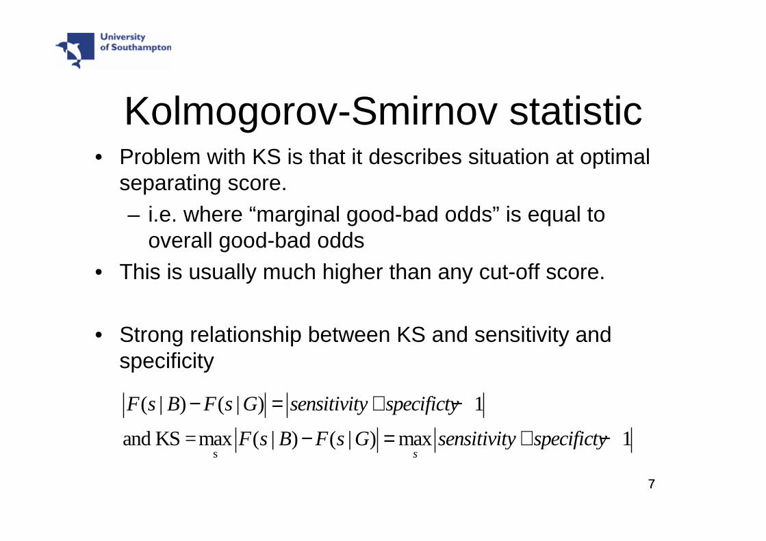
Kolmogorov-Smirnov statistic• Problem with KS is that it describes situation at optimal
separating score. – i.e. where “marginal good-bad odds” is equal to
overall good-bad odds • This is usually much higher than any cut-off score.
• Strong relationship between KS and sensitivity and specificity
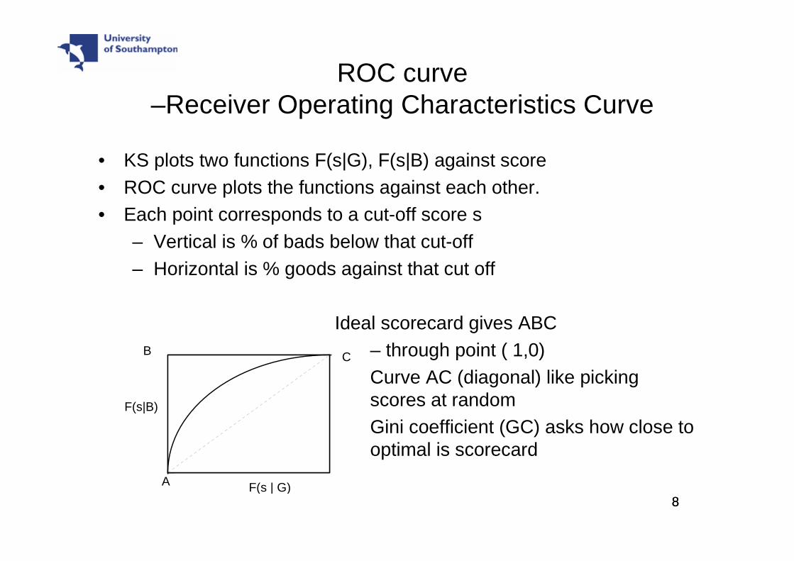
• KS plots two functions F(s|G), F(s|B) against score• ROC curve plots the functions against each other.• Each point corresponds to a cut-off score s
– Vertical is % of bads below that cut-off– Horizontal is % goods against that cut off
Ideal scorecard gives ABC– through point ( 1,0)Curve AC (diagonal) like picking scores at random Gini coefficient (GC) asks how close to optimal is scorecard
A
C
F(s | G)
F(s|B)
B
99
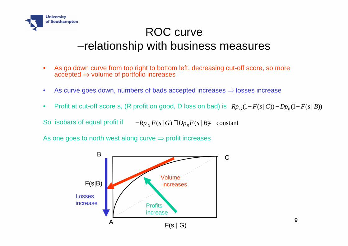
ROC curve –relationship with business measures
• As go down curve from top right to bottom left, decreasing cut-off score, so more accepted ⇒ volume of portfolio increases
• As curve goes down, numbers of bads accepted increases ⇒ losses increase
• Profit at cut-off score s, (R profit on good, D loss on bad) is
So isobars of equal profit if
As one goes to north west along curve ⇒ profit increases
(1 ( | )) (1 ( | ))G BRp F s G Dp F s B− − −
A
C
F(s | G)
F(s|B)
B
( | ) ( | ) constantG BRp F s G Dp F s B− + =
Volumeincreases
Lossesincrease Profits
increase
1010
Gini Coefficient
•Gini coefficient, GC, is 2x(ratio of area between curve and diagonal to area ABC)
•If GC =1 then perfect discrimination; GC =0 no discrimination.
•AUROC is area under the ROC curve so•GC= 2(AUROC -0.5)= 2AUROC -1
•K-S is greatest vertical distance from diagonal to curve.•
A
C
F(s | G)
F(s|B)
B
F(s|B)
F(s|G)
1111
Lift curve and Accuracy Ratio AR
• Lift curve looks similar to ROC curve ( originated in marketing) but subtle differences
• Plots F(s|B) % bads rejected against F(s) % rejected• Ideal scorecard gives ABC ( B is pB of population in)• Random scorecard given by diagonal AC• Curve depends on population odds• BUT Accuracy ratio, AR = 2( area curve above diagonal)/area ABC
• AR = GC ( even though different curves)
F(s)
F(s|B)
A
CB
1212
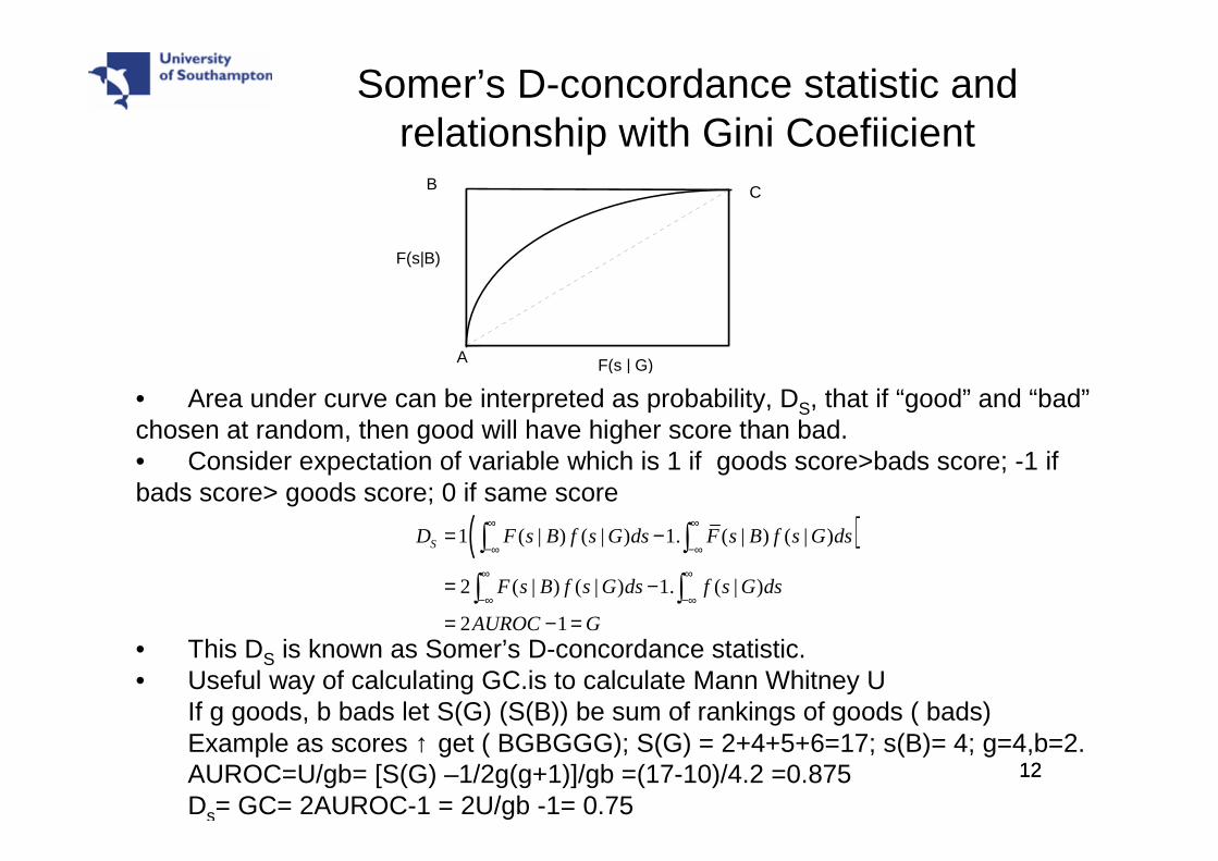
Somer’s D-concordance statistic and relationship with Gini Coefiicient
A
C
F(s | G)
F(s|B)
B
• Area under curve can be interpreted as probability, DS, that if “good” and “bad”chosen at random, then good will have higher score than bad. • Consider expectation of variable which is 1 if goods score>bads score; -1 if bads score> goods score; 0 if same score
• This DS is known as Somer’s D-concordance statistic. • Useful way of calculating GC.is to calculate Mann Whitney U
If g goods, b bads let S(G) (S(B)) be sum of rankings of goods ( bads) Example as scores ↑ get ( BGBGGG); S(G) = 2+4+5+6=17; s(B)= 4; g=4,b=2.AUROC=U/gb= [S(G) –1/2g(g+1)]/gb =(17-10)/4.2 =0.875 Ds= GC= 2AUROC-1 = 2U/gb -1= 0.75
( )1 ( | ) ( | ) 1. ( | ) ( | )
2 ( | ) ( | ) 1. ( | )
2 1
SD F s B f s G ds F s B f s G ds
F s B f s G ds f s G ds
AUROC G
∞ ∞
−∞ −∞
∞ ∞
−∞ −∞
= −
= −
= − =
∫ ∫
∫ ∫
1313
C
A
B
D
F
Very Simple bound on Gini and its powerful consequences
• Assume the scorecard has monotonically increasing marginal odds (reasonable)⇔ ROC curve is concave
• Area of AFE = (b-g)AG/2; • Area of FEC= (b-g).GD/2• Area of two triangles = (b-g)/2 < area from curve to diagonal =GC/2• GC> (b-g) for any point on the curve
(g,b)=(F(s|G,F(s|B)
E
G
C
1414
• GC > ( b-g)
• Take (g,b) to be at s which Maximises |F(s|B)-F(s|G)|, ⇔ GC > KS
• Good cards satisfy 50-10 rule ( pick up 50% of bads in first 10% of goods)
• 50-10 rule ⇒ G> .4
A
B
D
F
Very Simple bound on Gini and its powerful consequences
(g,b)=(F(s|G,F(s|B)
E
1515
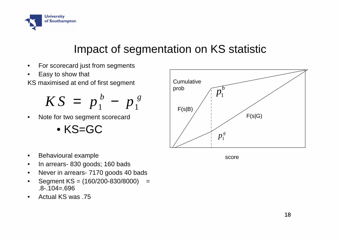
Segmentation and Discrimination• In reality a scoring system consists of not just one score
card but a suite of scorecards built on different segments of the population.
• Reasons for segmentation– System / data constraints – new account vs older accounts– Policy issues – want young people - different scorecard for <25’s– Significant interactions between variables and others
• Usually only calculate discrimination measure for each scorecard separately but should do it for whole system after scorecards have been calibrated on common scale
• How much of the discrimination is due to the scorecards and how much to the segmentation?
1616
Measuring power of segmentation in scorecards
• Measure segmentation power by taking the segments and choose scorecards which discriminates no better than random in each segment.
• Give borrower j in segment i a score of si +εuj where uj has uniform distribution on [0,1] and si+1 > si + ε
• Results for two segment case but expands to k segment case.• Assume segment 1 has g1 goods and b1 bads , score s1
and segment 2 has g2 goods and b2 bads, score s2 and assume
• Let
• Define
1 2
1 2
g g
b b<
1 1 1 2 2 2
b b g g1 2 1 21 2 1 2
1 2 1 2 1 2 1 2
t t1 21 2
1 2 1 2
; ;
; ; ;
;
n g b n g b
b b g gp p p pb b b b g g g g
n np pn n n n
= + = +
= = = =+ + + +
= =+ +
1717
Impact of segmentation on Gini coefficient• AEC is ROC curve for segmented/random Gini
• Example from behavioural scorecards – where can segment on whether ever in arrears or not
• In arrears- 830 goods; 160 bads• Never in arrears- 7170 goods 40 bads• Segment Gini = (160/200-830/8000) = .8-.104=.696• Actual Gini was .88
• Even if no segmentation,gives view of how much of Gini, this characteristic brings to scorecard.
– Is like using (approx) D-concordance to decide which variables to choose
• Explains why behavioural, scores have higher Ginis than application score
– In example suppose Gini for no arrears is like that for application score say GC; assume cannot distinguish good/bads in arrears , then provided arrears score is small enough so curve goes through E
For segmentation just by itself D = 4.273Actual D = 5.761 ( but done using equal variance approx)
( ) ( )22 22
2 2 2 2
2 21 2 1 2 2 1 1 2 2 1 1 2
1 2 1 2
1 1 1
2 2
( ) ( ) ( )
2
G B
G BG B G B
g g b b g b g b g g b b
b b g g
D
p p p p p p p p p p p p
p p p p
σ σµ µ
σ σ σ σ−
= + − +
+ − + −=
2121
Conclusions• There are connections between the different ways of measuring the
discrimination of scorecards• ROC curve is most fundamental of the measures ( does not depend
on population odds) includes KS and D-concordance• Very simple triangle bound give quick indication of GC• Shows GC>KS• Triangle bound is actual value if one only segments with random
scorecard in each segment• Allows one to recognise how much discrimination is built into
segmentation alone independent of scorecards then built• Even if no segmentation, gives importance of the variable
considered for segmentation in full population scorecard