Page 1
Georgia State UniversityScholarWorks @ Georgia State University
Marketing Dissertations Department of Marketing
7-31-2015
Measuring the Lifetime Value of a Customer in theConsumer Packaged Goods (CPG) industrySarang SunderGeorgia State University
Follow this and additional works at: http://scholarworks.gsu.edu/marketing_diss
This Dissertation is brought to you for free and open access by the Department of Marketing at ScholarWorks @ Georgia State University. It has beenaccepted for inclusion in Marketing Dissertations by an authorized administrator of ScholarWorks @ Georgia State University. For more information,please contact [email protected] .
Recommended CitationSunder, Sarang, "Measuring the Lifetime Value of a Customer in the Consumer Packaged Goods (CPG) industry." Dissertation,Georgia State University, 2015.http://scholarworks.gsu.edu/marketing_diss/30
Page 2
1
PERMISSION TO BORROW
In presenting this dissertation as a partial fulfillment of the requirements for an advanced degree
from Georgia State University, I agree that the Library of the University shall make it available
for inspection and circulation in accordance with its regulations governing materials of this type.
I agree that permission to quote from, to copy from, or publish this dissertation may be granted
by the author or, in his/her absence, the professor under whose direction it was written or, in his
absence, by the Dean of the Robinson College of Business. Such quoting, copying, or publishing
must be solely for the scholarly purposes and does not involve potential financial gain. It is
understood that any copying from or publication of this dissertation which involves potential
gain will not be allowed without written permission of the author.
SARANG SUNDER
Page 3
2
NOTICE TO BORROWERS
All dissertations deposited in the Georgia State University Library must be used only in
accordance with the stipulations prescribed by the author in the preceding statement.
The author of this dissertation is:
SARANG SUNDER
Georgia State University,
Tower Place 200, Suite 204,
3348 Peachtree Rd NE,
Atlanta, GA- 30326
The director of this dissertation is:
DR. V. KUMAR
DEPARTMENT OF MARKETING
Georgia State University,
Tower Place 200, Suite 204,
3348 Peachtree Rd NE,
Atlanta, GA- 30326
Page 4
3
MEASURING THE LIFETIME VALUE OF A CUSTOMER IN THE
CONSUMER PACKAGED GOODS (CPG) INDUSTRY
BY
SARANG SUNDER
A Dissertation Submitted in Partial Fulfillment of the Requirements for the Degree
Of
Doctor of Philosophy
In the Robinson College of Business
Of
Georgia State University
Page 5
4
GEORGIA STATE UNIVERSITY
ROBINSON COLLEGE OF BUSINESS
2015
Page 6
5
Copyright by
SARANG SUNDER
2015
Page 7
6
ACCEPTANCE
This dissertation was prepared under the direction of SARANG SUNDER’S Dissertation
Committee. It has been approved and accepted by all members of that committee, and it has
been accepted in partial fulfillment of the requirements for the degree of Doctoral of Philosophy
in Business Administration in the J. Mack Robinson College of Business of Georgia State
University.
RICHARD PHILLIPS, DEAN
DISSERTATION COMMITTEE
DR. V. KUMAR (CHAIR)
DR. YI ZHAO
DR. DENISH SHAH
DR. ROBERT P. LEONE
Page 8
7
ABSTRACT
MEASURING THE LIFETIME VALUE OF A CUSTOMER IN THE CONSUMER
PACKAGED GOODS (CPG) INDUSTRY
BY
SARANG SUNDER
JULY 8TH, 2015
Committee Chair: DR. V. KUMAR
Major Academic Unit: MARKETING
In this study, we propose a flexible framework to assess Customer Lifetime Value (CLV)
in the Consumer Packaged Goods (CPG) context. We address the substantive and modeling
challenges that arise in this setting, namely (a) multiple-discreteness, (b) brand-switching, and
(c) budget constrained consumption. Using a Bayesian estimation, we are also able to infer the
consumer’s latent budgetary constraint using only transaction information, thus enabling
managers to understand the customer’s budgetary constraint without having to survey or depend
on aggregate measures of budget constraints. Using the proposed framework, CPG
manufacturers can assess CLV at the focal brand-level as well as at the category-level, a
departure from CLV literature which has mostly been firm-centric. We implement the proposed
model on panel data in the carbonated beverages category and showcase the benefits of the
proposed model over simpler heuristics as well as conventional CLV approaches. Finally, we
conduct two policy simulations describing the role of the budget constraint on CLV as well as
the asymmetric effects of pricing in this setting and develop managerial insights in this context.
Keywords: Customer Relationship Management (CRM), Structural models, Bayesian
estimation, Consumer Packaged Goods (CPG), Multiple discreteness, Customer Lifetime Value
(CLV), Budget constraints
Page 9
8
ACKNOWLEDGEMENTS
I would not be where I am without the unwavering support of my family, committee
members, advisers, fellow PhD students and friends. I greatly appreciate their belief and
confidence in me. I would like to express my deepest gratitude to my advisor, Dr. V. Kumar
(VK) who has been instrumental in molding me as a researcher from the day I met him. I will be
forever grateful to VK for taking me under his wing, mentoring and believing in me through my
years as a PhD (and Masters) student. I will always look up to him for advice and a source for
inspiration as I build my career in this discipline. I thank my dissertation committee of Dr. Yi
Zhao, Dr. Robert Leone and Dr. Denish Shah who have advised and supported me over the years
both professionally and personally. I am also extremely grateful to my friends and fellow PhD
students at the Center for Excellence in Brand and Customer Management (CEBCM) many of
whom have been my sounding board for research ideas and have in general made my work days
more fun and enjoyable. Because of them and my professors, my doctoral experience at GSU has
been one I will always deeply cherish.
I am extremely thankful to my family who have stuck with me through my highs and lows.
I thank my parents, Sunder and Usha, for supporting me and remaining so confident in me no
matter the path that I choose. I thank my brother Shyam and my grandparents Appappa,
Bigamma and Samboo paati who, each in their own ways, have supported me and given me
encouragement throughout. I also owe a debt of gratitude to Ranjini and Kedar who have advised
me and have remained close confidants through the years. Finally, my journey as a PhD student
would have never been completed without the love, support and patience of my wife, Anu. She
has always been right beside me, proof reading my papers, being a soundboard for my ideas and
supporting me throughout. Her reassuring voice and calming presence has kept me going through
thick and thin. It is difficult to fail (no matter how challenging the task) when you have so many
people who truly believe in you.
Page 10
9
TABLE OF CONTENTS
INTRODUCTION ........................................................................................................................ 11 LITERATURE GAP ..................................................................................................................... 16
Customer Lifetime Value (CLV) modeling .................................................................... 16 Level of Aggregation ................................................................................................... 17 Competition in CLV modeling ..................................................................................... 18 Choice, Quantity, & Timing Modeling ........................................................................ 19
Models of multiple discreteness ...................................................................................... 21 DATA ........................................................................................................................................... 22
Model Free Analyses ....................................................................................................... 23 Multiple-discreteness check ............................................................................................ 25
METHODOLOGY ....................................................................................................................... 26 The Budget Constraint in the CPG context ..................................................................... 27 Consumer’s Utility Specification .................................................................................... 28 Heterogeneity .................................................................................................................. 32 Likelihood ....................................................................................................................... 32 Model Identification ........................................................................................................ 34 Estimation........................................................................................................................ 35 Variable Operationalization ............................................................................................ 36
State Dependence: ....................................................................................................... 36 Past purchase behavior ............................................................................................... 37
RESULTS ..................................................................................................................................... 39 Simulation Study ............................................................................................................. 39 Model Evaluation & Performance................................................................................... 39 Findings from Model Estimation .................................................................................... 41
Consumer’s Budget constraint. ................................................................................... 41 Inertia effects ............................................................................................................... 42 Brand-specific effects .................................................................................................. 42
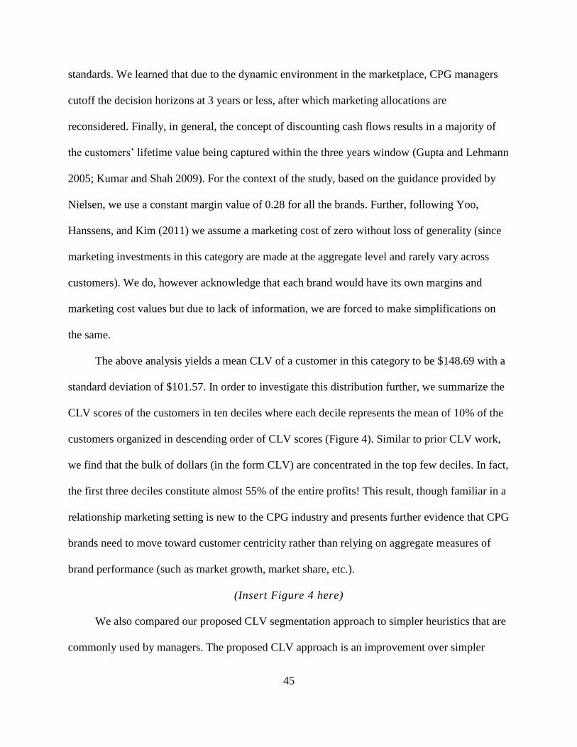
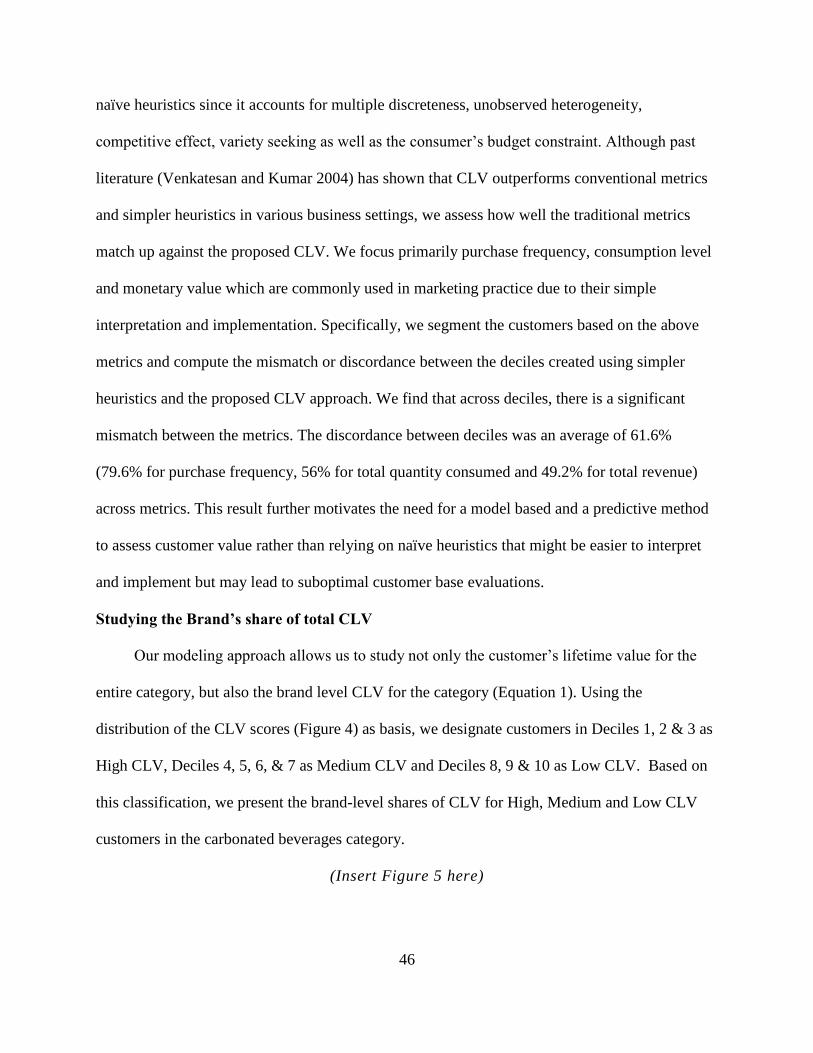
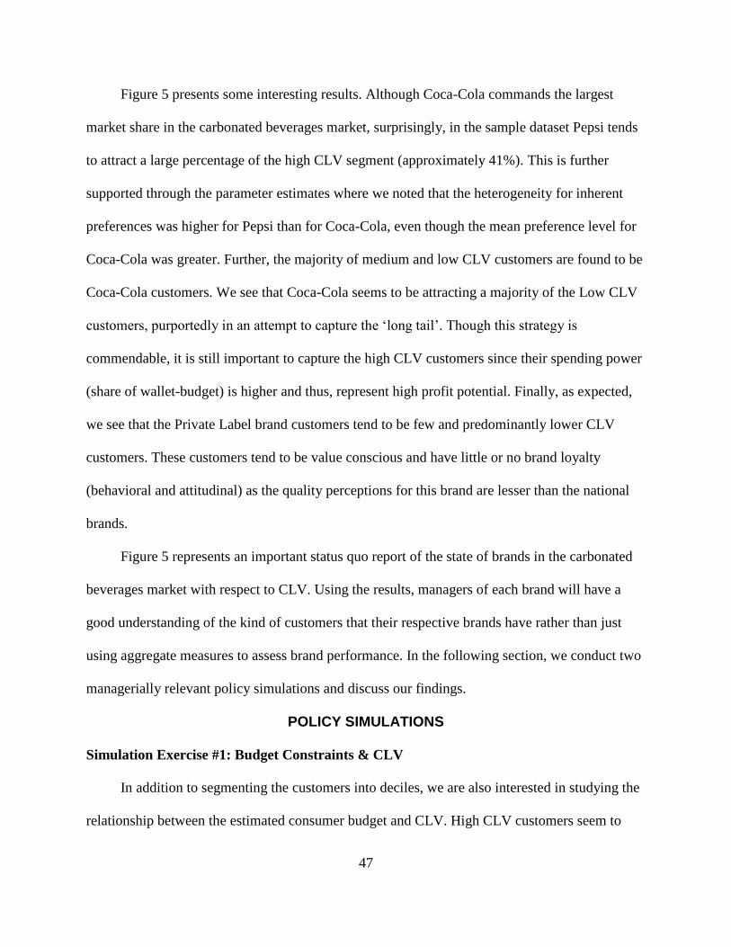
CLV IN THE CARBONATED BEVERAGES CATEGORY ..................................................... 44 CLV Measurement .......................................................................................................... 44 Studying the Brand’s share of total CLV ........................................................................ 46
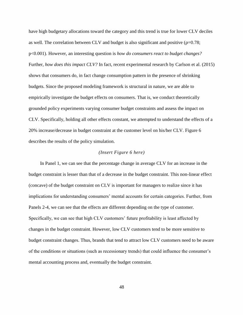
POLICY SIMULATIONS ............................................................................................................ 47 Simulation Exercise #1: Budget Constraints & CLV...................................................... 47 Simulation Exercise #2: Pricing & Consumption ........................................................... 49
DISCUSSION ............................................................................................................................... 51 IMPLEMENTING CLV IN THE CPG CONTEXT ..................................................................... 53
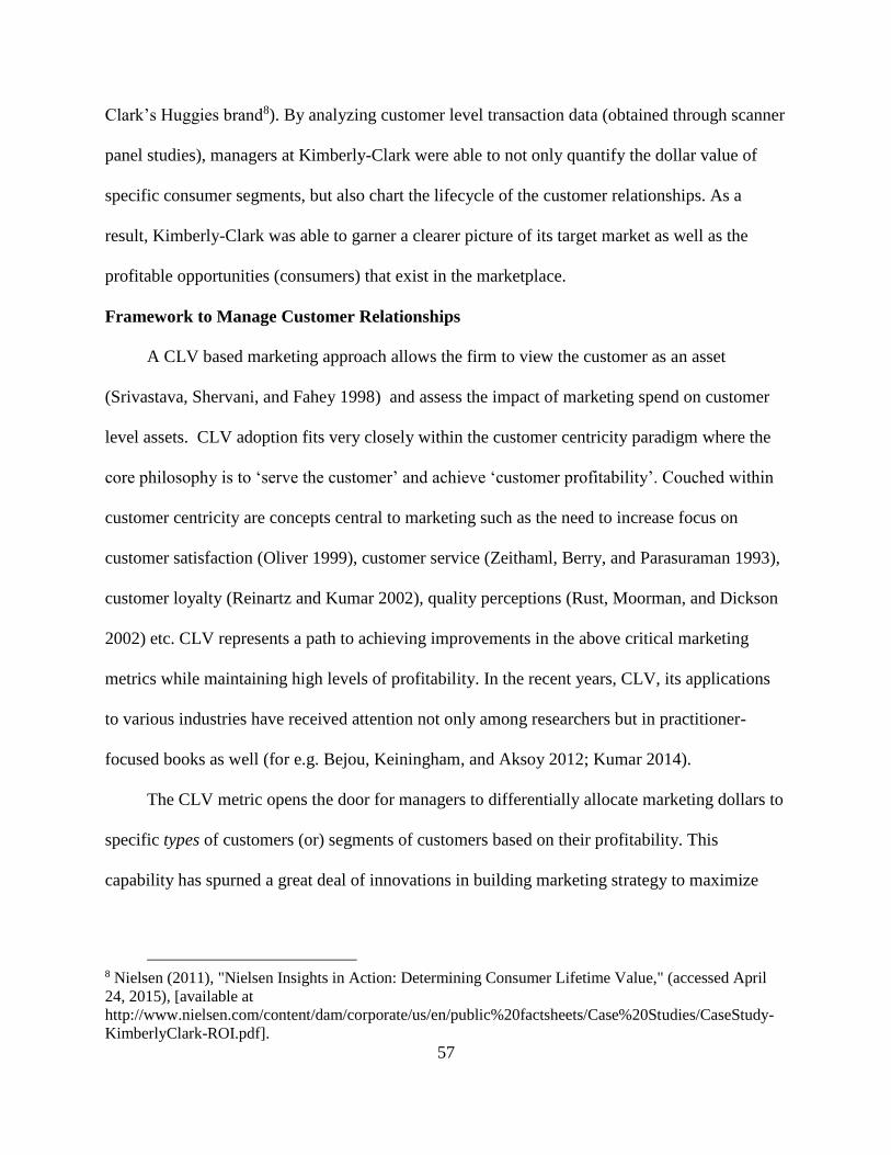
Embracing the Customer-centricity Paradigm ................................................................ 55 Framework to Manage Customer Relationships ............................................................. 57 Linking Marketing to Firm Value ................................................................................... 58
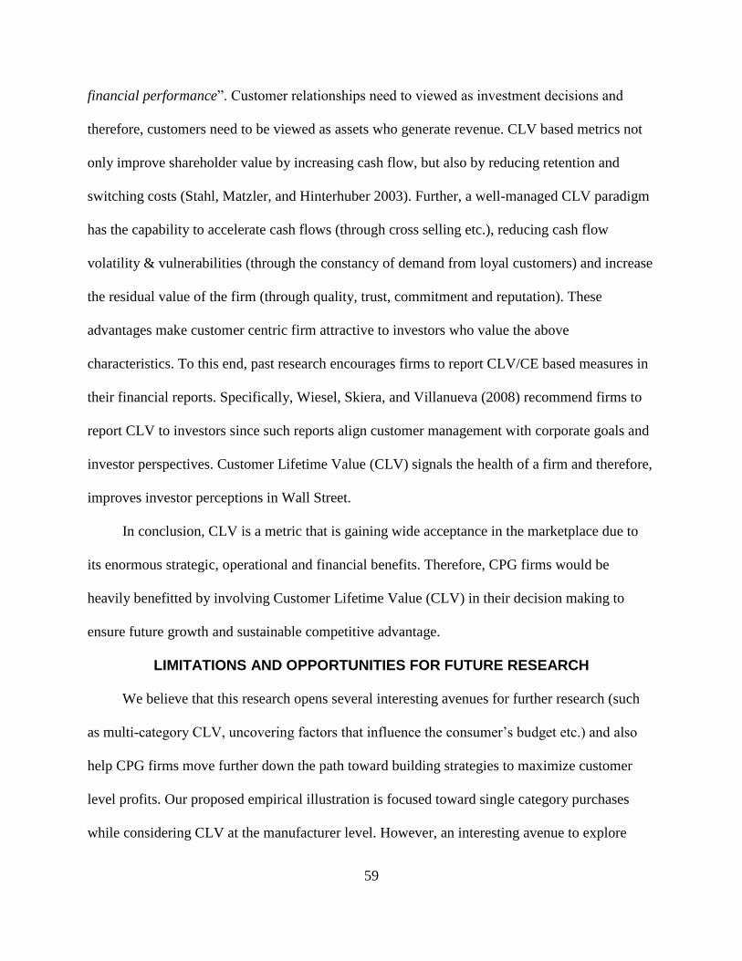
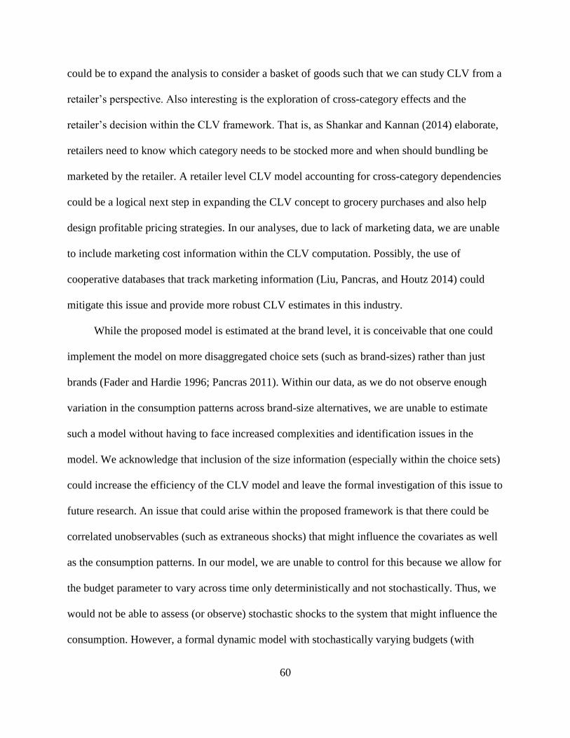
LIMITATIONS AND OPPORTUNITIES FOR FUTURE RESEARCH .................................... 59 REFERENCES ............................................................................................................................. 62 TABLES AND FIGURES ............................................................................................................ 69 APPENDIX A- MODEL IDENTIFICATION ............................................................................. 81 APPENDIX B- ESTIMATION ALGORITHM ........................................................................... 84
Step 1: Data Augmentation & Gibbs sampling ............................................................... 84
Page 11
10
Generate ψijt|αij, δi, yi, βj ........................................................................................... 84
Generate αij, ................................................................................................................ 85 Step 2: M-H Algorithm ................................................................................................... 85
APPENDIX C- THE GIBBS SAMPLER ..................................................................................... 87 Priors ............................................................................................................................... 87 Conditional Posteriors ..................................................................................................... 88
APPENDIX D- SIMULATION STUDY ..................................................................................... 91 APPENDIX E- BENCHMARK MODEL SPECIFICATION ...................................................... 93 APPENDIX F- RESULTS OF SIMULATION EXERCISE #2 ................................................... 94
LIST OF TABLES AND FIGURES
Table 1- Prior literature on CLV ................................................................................................... 69 Table 2- Incidence of Multiple discreteness in data ..................................................................... 70 Table 3- Variable Operationalization ............................................................................................ 71 Table 4- Summary Statistics of Relevant Variables ..................................................................... 72 Table 5- Model Performance ........................................................................................................ 73 Table 6- Budget and State Dependence Parameter Estimates ...................................................... 74 Table 7- Brand-Specific Parameter Estimates for Baseline Utility .............................................. 75 Table 8- Own- and Cross-effects of Price..................................................................................... 76 Table 9- Price effects across CLV segments (Coca-Cola) ............................................................ 76 Table 10- Simulation Study Results ............................................................................................. 91 Table 11- Impact of 10% change in Dr. Pepper Price .................................................................. 94 Table 12- Impact of 10% change in Pepsi Price ........................................................................... 94 Table 13- Impact of 10% change in Private Label Price .............................................................. 94
Figure 1- Time Trends in Key Variables ...................................................................................... 77 Figure 2- Histogram describing Customer-level Purchase Distribution ....................................... 78 Figure 3- Bayesian Estimation Strategy ....................................................................................... 79 Figure 4- Distribution of Category-level CLV ............................................................................. 79 Figure 5- Brand share of Category-level CLV ............................................................................. 80 Figure 6- Counterfactual #1: Impact of the Budget Constraint on CLV ...................................... 80
Page 12
11
INTRODUCTION
The customer-centricity paradigm has long been documented as being one of the most
important tenets of effective marketing in today’s dynamic environment. With the advent of
technology and Customer Relationship Management (CRM), there is an explosion of
disaggregate and granular customer data (transactional as well as survey) available to firms.
Research has proposed several methods and metrics to evaluate the customer such as Recency-
Frequency-Monetary value (RFM) (Cheng and Chen 2009), Share of Wallet, Past Customer
Value (PCV), etc. In the past decade, Customer Lifetime Value (CLV) has emerged as an
effective metric for CRM and a leading indicator of customer engagement with the firm (Kumar
2014). Customer Relationship Management (CRM) strategies developed from CLV modeling
has led to positive financial gains in Business-to-Business (B2B) as well as Business-to-
Consumer (B2C) settings (Kumar and Shah 2009; Villanueva and Hanssens 2007). Since the
CLV metric is heavily dependent on customer relationships and transaction data, it has mostly
been implemented in the relationship-marketing settings. However, the concepts of CLV and
customer-centric marketing are applicable in traditionally product-centric industries such as
consumer packaged goods (CPG) as well. In fact, the implementation of CLV in the consumer
packaged setting is one of the explicitly stated objectives of the Marketing Accountability
Standards Board (MASB)1.
However, traditional marketing (especially in the CPG context) has focused on reaching
out to consumers through mass marketing and delivering standardized products/services. While
this has worked in the past, it may no longer be sustainable in a dynamic and digitally connected
marketing environment. Although traditionally used aggregate metrics (such as market share,
1 http://www.themasb.org/projects/underway/
Page 13
12
sales volume, revenue etc.) which are commonly used in the CPG context to assess brand
performance convey important information about the product/brand and can be readily
calculated, they do not provide us with the complete picture. While aggregate metrics give
managers an indication of the health of the brand and serve as an ‘aggregate’ proxy for
performance, they do not provide any information regarding which customers grew and which
ones did not.
Further, flow based metrics (such as market share, brand sales etc.) are very sensitive to
extraneous shocks (Yoo, Hanssens, and Kim 2011) and ignore the heterogeneity present among
households. CLV presents stability based on consumer behavior which is long-term focused and
forward looking in nature. CPG firms are investing heavily in innovations in CRM that would
move them closer to a CLV-based approach to decision making. While there are several case
studies and white papers hinting at the need for customer centricity in CPG industry, to our
knowledge, there is no academic study providing a robust methodology to assess CLV in the
CPG industry. Through this research, we hope to provide the first step in applying customer
valuation and customer centric marketing in the CPG industry.
In order to assess CLV in the CPG industry, we need to build a model that accurately
captures consumer’s decision making in this setting. The implementation of a CLV-based
marketing paradigm in CPG firms is faced with several challenges such as (a) multiple
discreteness problem (where consumers make more than one brand in the same occasion), (b)
heavy brand switching and (c) budget constrained nature of CPG purchases. First, CPG
consumers2 do not always purchase a single brand in a given month. Due to the relatively lower
2 In this study, we use “consumer”, “customer” and “household” interchangeably. Our model is
implemented at the household level, but we note that the model is flexible to be estimated at the consumer
level if the data were available.
Page 14
13
(relative to relationship driven CLV contexts) costs of switching in the CPG industry (Carpenter
and Lehmann 1985), variety seeking consumers tend to try various brands within the same
shopping period, thus leading to multiple discreteness in CPG consumption which has been
documented in the literature (Allender et al. 2013; Dubé 2004; Richards, Gómez, and Pofahl
2012). This multi-brand purchase in the same given month leads to violations of typical discrete
choice models which are commonly used in conventional CLV models. This presents the first
challenge wherein, in order to accurately capture the consumption patterns, the CLV model
needs to account for multiple discreteness.
Second, given the low cost of switching, we need to explicitly account for brand switching
and competing brand effects in the CPG context. Previous research has highlighted the
importance of accounting for brand switching in CPG markets, especially in situations of low
product differentiation (van Oest 2005). A relatively small price promotion in one week could
induce customers to switch brands and consume another product (Bell, Chiang, and
Padmanabhan 1999; Sun, Neslin, and Srinivasan 2003). However, conventional CLV models
which rely on internal company data often ignore the role of competition and brand switching.
Extant CLV models that do account for brand switching rely heavily on survey data describing
either the customer’s actual switching (Rust, Lemon, and Zeithaml 2004) or Share of Wallet
information. (Kumar and Shah 2009). The collection of survey data, while viable in business
setting where relationships are clearly defined, becomes very challenging in the CPG context due
to scale and cost issues associated with appending panel data with survey information.
Third, existing evidence in consumer behavior as well as economics shows that households
keep track of category-specific budgets especially in the CPG setting (Antonides, Manon de
Groot, and Fred van Raaij 2011; Heath and Soll 1996; Stilley, Inman, and Wakefield 2010) and
Page 15
14
try to maintain category spending (focal product category + outside substitutes) within a target
maximum level, so as to have control over consumption or spending (Gilboa, Postlewaite, and
Schmeidler 2010). That is, consumers have unobserved limits on the amount of dollars that they
are willing to allocate toward a specific category, which includes the product category as well as
outside substitute goods. For example, a consumer could view water, juice and carbonated soda
as substitutes and allocate dollars toward this ‘mental’ category (focal product category as well
as substitutes outside the product category). The budget constraint would then be encompassing
all the dollars allocated toward this overall spending category. In the economics literature,
Hastings and Shapiro (2013) explore this phenomenon of mental category-specific budgets using
panel data from a US retailer and show that a category level budgeting predicts customer
behavior quite well. The idea of mental budgeting and mental accounting was first proposed by
Thaler (1985) as a theoretical model of consumer behavior and later used in marketing literature
(Cheema and Soman 2006; Heath and Soll 1996). Prelec and Loewenstein (1998) point out that
when consumers make purchases they often experience a pain of buying, which acts as a
counterbalance for the pleasure of consumption. Mental budgets act as a form of self-control to
ensure that they stay within the spending limits at the category level (and thus, at the grocery trip
level). However, inferring the consumer’s latent mental ceiling/budget has proven to be
challenging. Much of past research in the area of mental budgeting has relied on some form of
survey data (Du and Kamakura 2008; Stilley, Inman, and Wakefield 2010). Since collecting and
appending survey data in the CPG setting is very difficult, it becomes necessary to infer this
information using readily available transaction data. This issue is further underscored when
addressing CLV in the CPG setting since managers need to know not only what the CLV of the
customer is, but also the maximum budget allocations that could be made within the category.
Page 16
15
Knowledge of the limits of a customer’s spend (budget constraints) helps managers avoid
overspending on customers who have a low ceiling and underspending on customers who have a
high ceiling. Our main research objectives are highlighted below,
1. Getting a long-term customer centric view of the CPG customer: How to model the
consumer’s CLV in a CPG setting?
2. Explicitly account for multiple discreteness and heavy brand switching: How to leverage
scanner panel data in the CPG industry to explicitly consider brand switching and account for
the multiple discreteness issue when modeling CLV?
3. Understanding the budgetary constraint: How to infer the customer’s budget constraint at the
individual level? This information would allow managers to assess the budgetary ceilings
that households impose for specific categories.
4. Policy Simulations in CLV modeling: How can firms use a structural approach to assess CLV
in the CPG setting and eventually conduct relevant counterfactuals without having to conduct
expensive studies in the field?
We implement a structural model of multiple discrete purchases on scanner panel
transaction data spanning across three years. We showcase the predictive power of our approach
relative to conventional CLV modeling approaches and also highlight its advantages over
simpler heuristics (such as usage, market share etc.). Additionally, we compute individual CLV
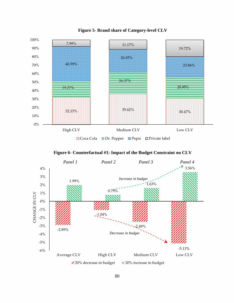
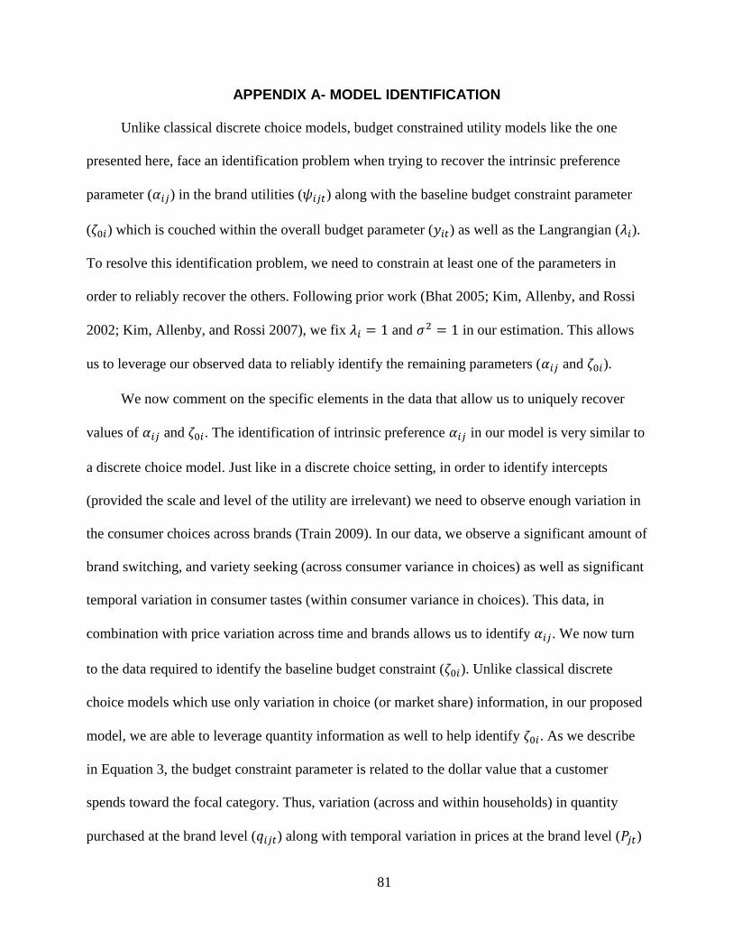
and segment the customers into high, medium and low CLV segments. At the segment level, we
provide insights into each CPG brand’s share of CLV and discuss the implications for each
brand. Finally, we conduct two policy simulations that are managerially relevant. First, we
simulate the effect of changes to the budget constraint on CLV. We find that, on average, a
reduction in the budget constraint leads to a greater effect in CLV than a gain in budget. We
Page 17
16
show that this effect is heterogeneous, that is, the magnitude of the effect is different depending
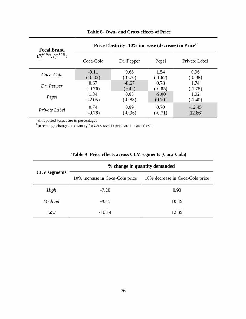
on CLV segment. Second, we study the own and cross effects of price on quantity consumed.
We find that the effects are non-symmetric for increases and decreases in price, indicating
nonlinear price elasticities. Further, as we highlight, this effect too is heterogeneous across CLV
segments.
The remainder of this article is organized in the following manner. In the next section, we
discuss the related marketing literature in the areas of CLV, and multiple discreteness modeling
and outline our contributions. Next, we provide a brief description of the data used in the
empirical application and present evidence of multiple discreteness in the data. Then, we develop
the structural model of multiple discreteness, discuss the operationalization of the budget
parameter, and derive the likelihood. Within this section, we also elaborate on the Bayesian
estimation procedure used to recover the parameters. Next, we elaborate on the findings from the
study and compare our model with conventional CLV models. In the subsequent section, we
compute the CLV, and conduct managerially relevant counterfactuals (or) policy simulations that
could aid CPG manufacturers in understanding CLV in the CPG setting. Finally, we highlight the
key academic and managerial implications of the proposed approach and conclude with
limitations and future research directions.
LITERATURE GAP
Customer Lifetime Value (CLV) modeling
CLV is an individual-level customer valuation metric that takes into account the total profit
contribution of a customer over his/her lifetime. It can be formally defined as the sum of the
cumulated cash flows- discounted using the weighted average cost of capital (WACC)- of a
customer over his/her entire lifetime (Kumar 2014). As is evident from the above definition,
Page 18
17
CLV measures the net worth of the customer. Since it is measured at the individual level,
companies that have computed CLV can now assess the distribution of their customer base
according to the potential value that they will achieve. The advantage of modeling the CLV from
a firm’s perspective is that the CLV metric gives the manager a view into the future profit
potential of the customer. Thus, by knowing the future profit potential of the customer, managers
can optimally allocate marketing dollars toward the right customers at the right time (Venkatesan
and Kumar 2004). Researchers have proposed several strategies (customer acquisition, retention
etc.) based on the CLV metric and have implemented these strategies in various industries such
as airlines, telecommunications, banking etc. It is to be noted that the past implementations of
CLV have been for industries with stronger customer relationships. Applying the CLV
framework to the CPG industry presents several practical challenges, the most important being
that the customer’s switching costs and brand loyalty are relatively lower. Since our focus is on
the CPG industry which is a B2C non-contractual setting, we will review the CLV literature that
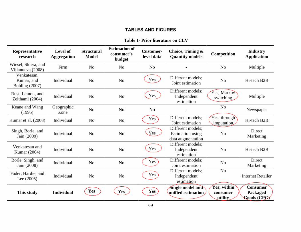
conforms to this setting. In Table 1, we outline the representative research in the CLV literature
and elaborate on the contributions of this study toward CLV modeling. There are mainly three
criteria that need to be addressed when reviewing the extant CLV literature, namely, (a) the level
of aggregation, (b) whether competition is included, (c) modeling approach and application. We
will discuss the following criteria in detail in the subsequent paragraphs.
(Insert Table 1 here)
Level of Aggregation: The level at which CLV/CE is computed depends on the kind of data that
is available to the researcher. As prior literature has stressed, the more disaggregate the data, the
more valuable the insights. Nevertheless, in certain situations, an aggregate view of CLV (either
at the territorial level or firm level) has proven to be quite beneficial to the firm. For example,
Page 19
18
Keane and Wang (1995) implement a lifetime value framework at the geographical level in a
newspaper setting and develop insights for the same. Several researchers have also used publicly
available data (such as company reports, third-party reports etc.) to evaluate the average CLV or
CE at the firm level. For example, Gupta, Lehmann, and Stuart (2004) propose a method to
estimate the average CLV of a customer for a firm using publicly available data while projecting
the revenue stream to an infinite horizon. This methodology was further improved and
substantiated by Wiesel, Skiera, and Villanueva (2008) by linking CE to shareholder value.
While firm-level estimation of CLV has immediate managerial advantages, it does not account
for the heterogeneity among the customers. Conducting a customer base analysis at the aggregate
level comes with its own risks. Specifically, ignoring heterogeneity in the CLV estimation can
lead to a consistent downward bias in elasticities and therefore under report the impact of
marketing on CLV (Fader and Hardie 2010). Given the richness of the data available to us and
the ‘structural’ evaluation of the model, we develop our modeling framework at the individual
customer level and therefore, explicitly account for heterogeneity in the customer base.
Competition in CLV modeling: Since consumers make choices relative to competing
brands/firms/offerings in the marketplace, it is important to evaluate the importance of
competition in CLV modeling especially in the CPG context. By failing to account for
competitive effects, CLV models could overestimate the impact of the firm’s own marketing
activities on CLV. Researchers have tried to mitigate this issue by including survey based
measures of the customer’s Share of Wallet (SOW) to control for competitive effects. However,
this approach has two shortfalls. First, it is difficult for the researcher to collect survey data for
the entire customer base and maintain the database for the entire transaction history of the
customer. Second, the SOW metric does not explicitly incorporate competition into the choice
Page 20
19
framework of the customer since it is used more as a control variable. Rust, Lemon, and
Zeithaml (2004) use a Markov switching matrix to account for the customer’s brand switching
tendencies. However, this method only considers the customer’s switching behavior but not
simultaneous purchasing behavior (purchasing from multiple brands at the same time). Further,
their approach relies heavily on the data gathered from large scale surveys of customers. This
may prove impractical in the CPG setting due to the cost structures associated with data
collection and inherent reporting biases within the survey data. The lack of consumption and
other marketing related data has proven to be very difficult to gather, especially in a CLV setting.
However, the rise of cooperative databases wherein data across multiple firms is pooled by third
party vendors has enabled researchers to have a clearer view of the customer. For example, Liu,
Pancras, and Houtz (2014) develop a framework for firms to manage customer acquisitions using
cooperative databases. Our approach to handling competition follows a similar perspective.
Leveraging data from third party vendors such as Nielsen/IRI, we directly including competition
within the consumer’s utility and implementing a unified CLV model on transaction data from
scanner panel data.
Choice, Quantity, & Timing Modeling: Previous research on CLV modeling has mostly relied on
separate specifications of choice, quantity and timing decision models to describe customer
decision making (Gupta et al. 2006; Kumar and Luo 2008). While these models have worked
well in situations where customer relationships are well defined, they may not be well suited for
the CPG context. A choice-then-quantity approach forces the researchers to make explicit
assumptions regarding the temporal ordering of decisions. In a CPG setting, this assumption may
not hold especially when consumers purchase more than one brand in the same purchase
occasion and switching costs are relatively low. Specification of separate choice, quantity and
Page 21
20
timing models could lead to parameter proliferation problems as well as the introduction of new
random utility error terms (for each decision model) into consumer preference (Chintagunta and
Nair 2011). Further, a reduced form approach of specifying joint models of multiple decisions
could suffer from the Lucas critique. This is true with dynamic models such as vector auto
regression models and other multivariate time series models which are commonly used in CLV
modeling. Thus, we propose a unified structural model which incorporates all of the above
consumer decisions within the same utility framework, thereby avoiding the parameter
proliferation problem while still modeling CLV.
In the CPG context, Yoo, Hanssens, and Kim (2011) merge a VAR based framework with
a stochastic model for customer behavior (BG/BB model from Fader, Hardie, and Shang (2010))
and provide valuable insights describing the evolution of customer equity in a CPG market. They
show that CE is much more stable and a better metric to use in the CPG market. This approach,
however, is applicable only for a one-brand-one-category setting and does not address the
multiple discreteness issue that is common in CPG purchases. For grocery product categories,
such as carbonated soft drinks, canned soup, pasta, cereals etc., households regularly purchase
assortments of brands (Allender et al. 2013; Dubé 2004; Kim, Allenby, and Rossi 2007;
Richards, Gómez, and Pofahl 2012) .This multiple discreteness issue violates the single-unit
purchase assumption of standard discrete choice models that past CLV models have been reliant
on. As we elaborate in the data section, handling the multiple discreteness issue is critical as
almost 40% of all transactions suffer from this problem in the carbonated soft drinks category.
Though the multiple discreteness issue has been studied in marketing literature in the past, it has
never been studied from a CLV perspective.
Page 22
21
Models of multiple discreteness
In the CPG setting, consumers tend to purchase assortments of products/brands in a
shopping trip, thus leading to the multiple discreteness problem. The multivariate Probit model
(Manchanda, Ansari, and Gupta 1999), which essentially treats the consumer choice decision as
a set of correlated binary choice models has been proposed to handle this issue without the use of
a structural modeling approach. While popular in marketing literature, this approach is
suboptimal when studying CLV since it does not make any conclusions regarding the quantity
decision, which is critical for CLV computation. Direct utility structural models which derive
demand from Karush-Kuhn-Tucker (KKT) conditions have been proposed as a viable alternative
to model multiple discreteness while taking advantage of the continuous nature of consumer
purchase. Variants of these models include those proposed by Kim, Allenby, and Rossi (2002),
Bhat (2008) as well as Satomura, Kim, and Allenby (2011) which rely on satiation to explain
multiple discreteness. An alternative approach in the economics literature was proposed by
Hendel (1999) who treats multiple discreteness as temporary variety seeking behavior. This
approach was later applied in marketing by Dubé (2004) to study demand in carbonated soft
drinks.
In the current study, we adopt a direct utility approach to structurally model multiple
discreteness while accounting for variety seeking behavior in the demand model. While falling
within the broader streams of multiple discreteness modeling and CLV, our work differs from
prior literature in the following ways. First, unlike previous literature (for e.g. Satomura, Kim,
and Allenby 2011) who have mostly used data from a controlled conjoint study (survey data), we
implement our model on a longitudinal transaction database in a CPG setting. Second, we allow
the budget parameter to deterministically vary with time (as a function of demographics, and
Page 23
22
seasonality effects) in our model so as to capture any time variations in the budget constraint
within the data. Finally, and most importantly, our main objective in this research is to apply a
multiple discrete modeling approach to predict the future profit stream of each customer (CLV)
across multiple brand purchases. In the next section, we describe the data in which the empirical
model was developed and implemented.
DATA
The empirical setting for the application of the proposed CLV model is the CPG industry.
Specifically, we used scanner panel data for carbonated beverages obtained from Nielsen/IRI in
our subsequent analyses. In the data, we observe monthly carbonated soft drink purchases at the
UPC level made by 40,098 consumers who were part of the Nielsen panel between the periods of
July 2007 and August 2010.
Next, we describe the criteria used in preparing the data in order to develop and estimate
the proposed model. First, a common challenge in modeling scanner panel data is to devise an
aggregation strategy such that a tractable set of choices/alternative are used for estimation
(Gordon, Goldfarb, and Li 2013). That is, too many alternatives in the data makes it
computationally cumbersome and also could lead to identification problems in the recovery of
parameters. We aggregated Universal Product Code (UPC) level data within the category into
manufacturer level brands. While it is possible to aggregate the data at the brand-size level
instead, we note that this leads to significant complications in our model as it requires the
estimation of several new parameters. Further, in our data there were a lot of customers who only
purchased a single size throughout the timeline of the data. Moreover, based on our
conversations with executives of one of the large CPG manufacturers in the dataset, we learned
that CLV at the brand level also carries significant value in this setting. We do, however note
Page 24
23
that our CLV model could accommodate more granular (brand-size) data provided there was
enough variation in consumption patterns. This yielded a dataset considering customer purchases
across four major brands (Coca Cola, Pepsi, Dr. Pepper and Private Labels) accounting for a
cumulative 89% of market share in the overall sample.
A second issue faced when building models using only customer-level scanner panel data
is that the researcher observes price only when the consumer makes a purchase of the focal
brand. In order to infer the missing price data for the other brands, we follow the heuristic
outlined by Gordon, Goldfarb, and Li (2013) and Erdem and Keane (1996). We imputed the
price information using purchases by other consumers in the same store type in the same month.
That is, when customer ‘i’ did not purchase brand ‘b’ at time ‘t’, we search the database for any
other customers ‘k’ (where k ≠ i) who purchased brand ‘b’ at time ‘t’ in a similar store type. We
then compute the average of the price across the ‘k’ to arrive at an imputed price which we use in
place of the missing information.
Model Free Analyses
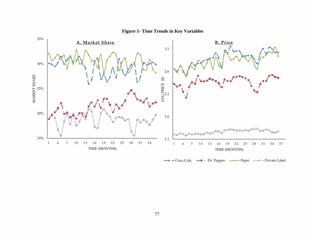
In the data, we observe temporal variations in brand purchases as well as prices. To
provide a deeper understanding of the data structure and patterns, we provide visual
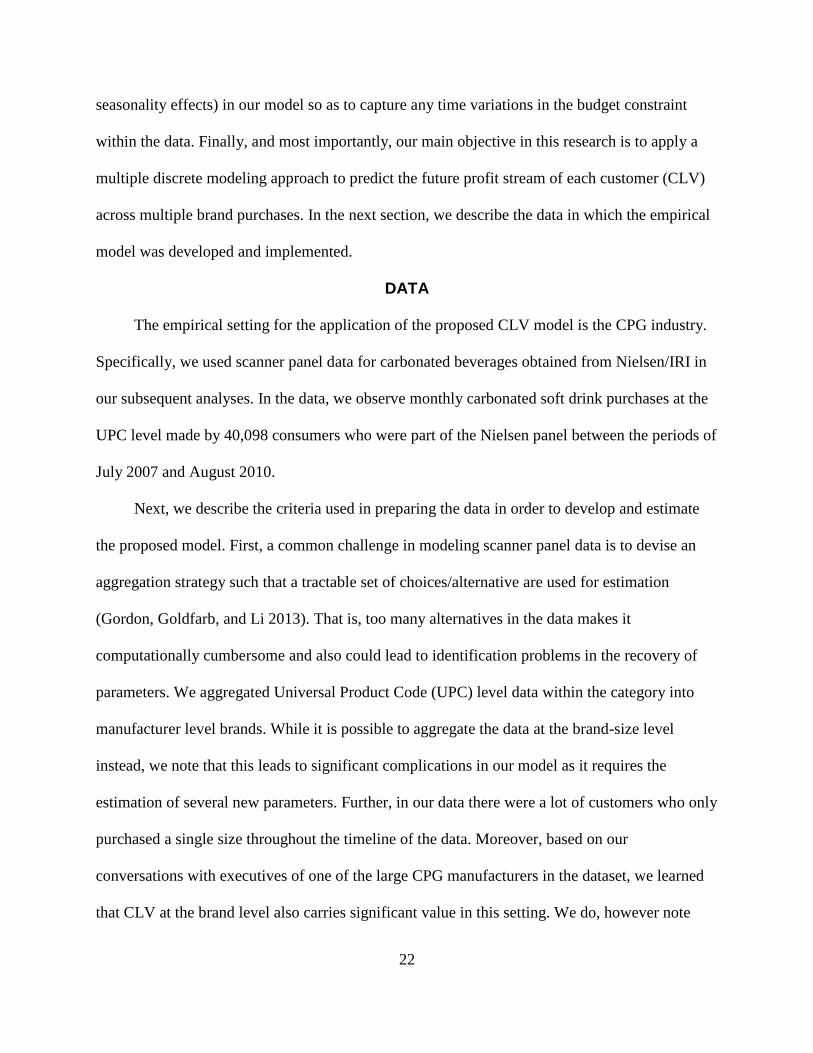
representations of key trends in the data. First, in Figure 1 (Panels A & B), we illustrate the time
trend in market share as well as price for the four major brands in the data. We can see that there
are two leaders in the market, Coca-Cola and Pepsi, who command an average of about 30%
market share. Visual inspection suggests that these two brands seem to be close competitors and
seem to steal market share from one another on a month to month basis. This is further supported
when we study the time trend of price data. On the other hand, we can see that Dr. Pepper’s
market share is increasing over time as is its price. The above trends indicate that there is
Page 25
24
significant competition between brands in this market and in addition to pricing, there are several
factors that could be influencing this.
(Insert Figure 1 here)
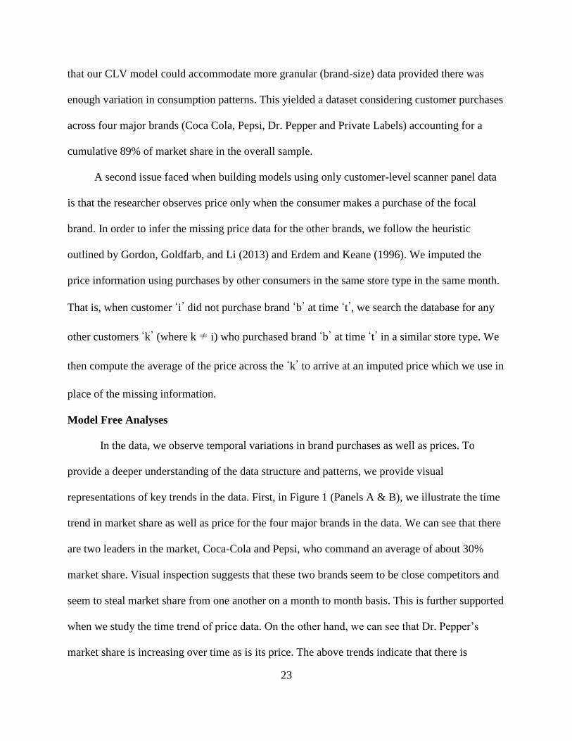
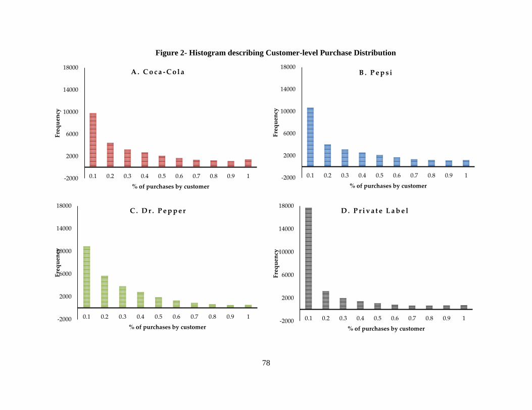
While aggregate metrics give managers an indication of the health of the brand and serve
as an ‘aggregate’ proxy for performance, they do not provide in-depth information regarding
which customers grew and which ones did not. Further, they do not address the inherent
heterogeneity among customer preferences to marketing. To illustrate this point, we compute
household level market share (the percentage of purchases of the focal brand relative to total
number of purchases). Figure 2 describes the distribution of household level market share across
the four major brands being considered. There are two key points to be noted in Figure 2. First,
there is a wide variation in customer purchases, suggesting that heterogeneity is indeed important
and needs to be considered.
(Insert Figure 2 here)
Second, the distribution of purchases across brands is also differences. A key question is
that when one brand decides to modify its price, how do the customers react? That is, given an
increase in price of Coca-Cola, the customer could (a) increase his purchase of another brand and
reduce his share of Coca-Cola purchases while still maintaining his overall consumption level, or
(b) continue to purchase Coca-Cola, but reduce the quantity consumed to remain within the
budget constraint. A model based approach (especially a structural model) is therefore, useful in
describing consumer decision making and reactions to observed changes in marketing. Overall,
the variations in the data help motivate the need to use a sophisticated modeling approach to
accurately address the above issues. In the following subsection, we further motivate the need for
Page 26
25
applying a multiple discreteness framework to the current context by providing evidence from
the data and literature.
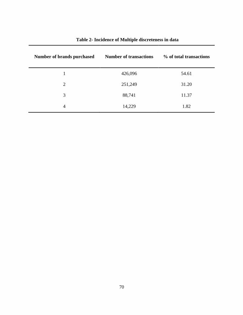
Multiple-discreteness check
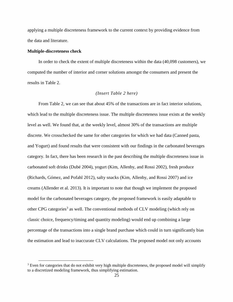
In order to check the extent of multiple discreteness within the data (40,098 customers), we
computed the number of interior and corner solutions amongst the consumers and present the
results in Table 2.
(Insert Table 2 here)
From Table 2, we can see that about 45% of the transactions are in fact interior solutions,
which lead to the multiple discreteness issue. The multiple discreteness issue exists at the weekly
level as well. We found that, at the weekly level, almost 30% of the transactions are multiple
discrete. We crosschecked the same for other categories for which we had data (Canned pasta,
and Yogurt) and found results that were consistent with our findings in the carbonated beverages
category. In fact, there has been research in the past describing the multiple discreteness issue in
carbonated soft drinks (Dubé 2004), yogurt (Kim, Allenby, and Rossi 2002), fresh produce
(Richards, Gómez, and Pofahl 2012), salty snacks (Kim, Allenby, and Rossi 2007) and ice
creams (Allender et al. 2013). It is important to note that though we implement the proposed
model for the carbonated beverages category, the proposed framework is easily adaptable to
other CPG categories3 as well. The conventional methods of CLV modeling (which rely on
classic choice, frequency/timing and quantity modeling) would end up combining a large
percentage of the transactions into a single brand purchase which could in turn significantly bias
the estimation and lead to inaccurate CLV calculations. The proposed model not only accounts
3 Even for categories that do not exhibit very high multiple discreteness, the proposed model will simplify
to a discretized modeling framework, thus simplifying estimation.
Page 27
26
for the above described multiple discreteness issue but also integrates the three main decisions
(choice, frequency/timing and quantity) within the same model.
METHODOLOGY
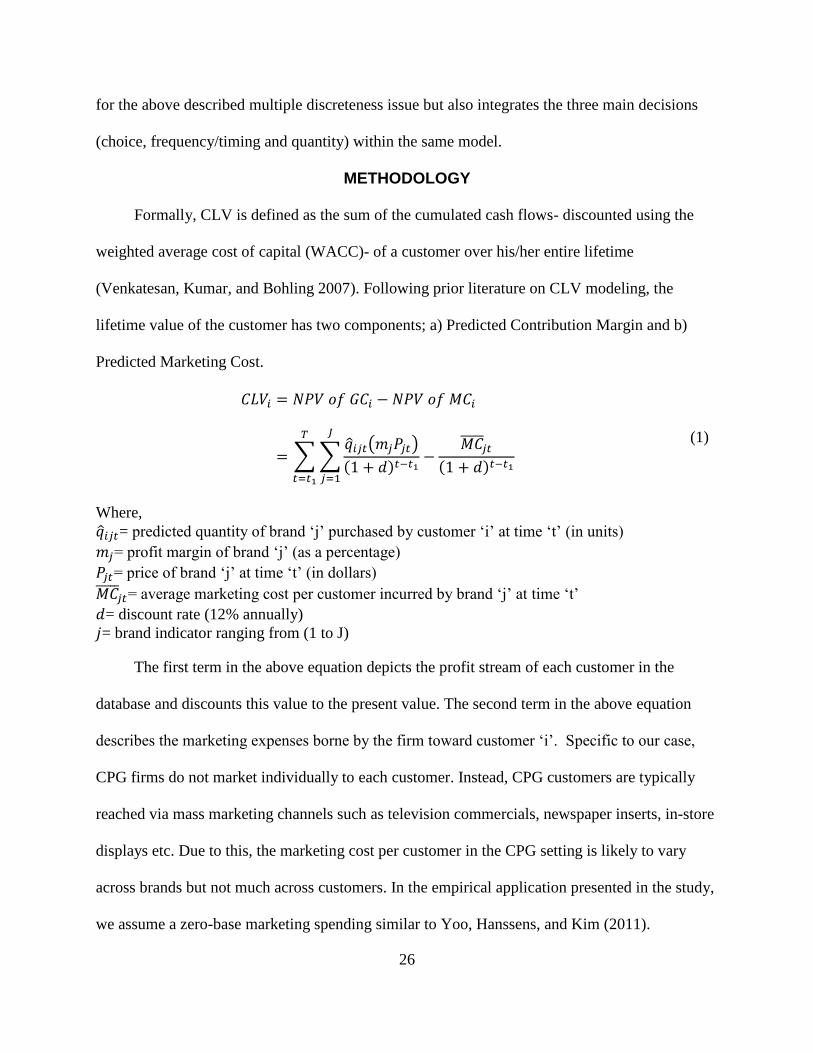
Formally, CLV is defined as the sum of the cumulated cash flows- discounted using the
weighted average cost of capital (WACC)- of a customer over his/her entire lifetime
(Venkatesan, Kumar, and Bohling 2007). Following prior literature on CLV modeling, the
lifetime value of the customer has two components; a) Predicted Contribution Margin and b)
Predicted Marketing Cost.
𝐶𝐿𝑉𝑖 = 𝑁𝑃𝑉 𝑜𝑓 𝐺𝐶𝑖 − 𝑁𝑃𝑉 𝑜𝑓 𝑀𝐶𝑖
= ∑ ∑�̂�𝑖𝑗𝑡(𝑚𝑗𝑃𝑗𝑡)
(1 + 𝑑)𝑡−𝑡1−
𝑀𝐶̅̅̅̅�̅�𝑡
(1 + 𝑑)𝑡−𝑡1
𝐽
𝑗=1
𝑇
𝑡=𝑡1
(1)
Where,
�̂�𝑖𝑗𝑡= predicted quantity of brand ‘j’ purchased by customer ‘i’ at time ‘t’ (in units)
𝑚𝑗= profit margin of brand ‘j’ (as a percentage)
𝑃𝑗𝑡= price of brand ‘j’ at time ‘t’ (in dollars)
𝑀𝐶̅̅̅̅�̅�𝑡= average marketing cost per customer incurred by brand ‘j’ at time ‘t’
𝑑= discount rate (12% annually)
𝑗= brand indicator ranging from (1 to J)
The first term in the above equation depicts the profit stream of each customer in the
database and discounts this value to the present value. The second term in the above equation
describes the marketing expenses borne by the firm toward customer ‘i’. Specific to our case,
CPG firms do not market individually to each customer. Instead, CPG customers are typically
reached via mass marketing channels such as television commercials, newspaper inserts, in-store
displays etc. Due to this, the marketing cost per customer in the CPG setting is likely to vary
across brands but not much across customers. In the empirical application presented in the study,
we assume a zero-base marketing spending similar to Yoo, Hanssens, and Kim (2011).
Page 28
27
Appending and re-estimating the framework along with marketing cost data will only improve
the CLV estimates, but not change our substantive conclusions. The model describing the
customer’s budget constrained utility maximization problem is presented below along with brief
discussions of each component.
In order to model the stochastic component (�̂�𝑖𝑗𝑡), we provide a structural approach
wherein the consumer maximizes his/her utility for each trip across a variety of brands. In order
to account for the multiple discreteness issue, we specify a direct utility model where consumers
are assumed to be utility maximizers subject to a budgetary constraint (or) monetary ceiling.
The Budget Constraint in the CPG context
In this subsection, we elaborate on the theoretical underpinnings of the budget constraint
construct, its boundaries and definition. Extant literature on mental accounting (Cheema and
Soman 2006; Thaler 1985) has shown that consumers impose restrictions on themselves to avoid
over spending and consumption. These restrictions are usually in the form of mental dollars that
consumers assign toward consumption and have been shown to exist in the grocery setting
(Milkman and Beshears 2009). In this study, we follow the view of Stilley, Inman, and
Wakefield (2010) who suggest that mental budgets for grocery trips are comprised of itemized
portions (or allocations at the brand/product level).
However, it is important to comment on the manner in which categorization could occur
within the consumer’s mindset. A valid criticism of imposing budget constraints at the category
level is that consumers do not always see substitutes within the category (as defined by the
brand/industry). Research in categorization (Antonides, Manon de Groot, and Fred van Raaij
2011; Ratneshwar, Pechmann, and Shocker 1996) has shown that consumers represent products
and substitutes differently. Thus, a model of consumer behavior (such as the one proposed in this
Page 29
28
study) that imposes a budget constraint at pre-defined category-level could be mis-specified
since it does not capture the substitution effects accurately. To overcome this difficulty, within
the model presented in this study (below), we specify the budget constraint (or) monetary ceiling
to be the maximum monies allocated by the consumer toward the focal category as well as
substitutes that may be considered outside the focal category. For example, the budget constraint
that we attempt to quantify in this study is the maximum dollars that the consumer allocates
toward the carbonated soft drinks category plus substitute product categories (such as water,
juice, etc.). We impose no restrictions on the manner in which these dollars are allocated across
substitutes. In the following section, we develop the consumer’s overall utility maximization
problem and describe the salient features of the model.
Consumer’s Utility Specification
The consumer’s overall utility (𝑈𝑖𝑡) can be expressed as a function of his/her utility from
consumption and category-level savings. The savings utility which tracks the overall spending
within the focal category as well as the budget constraint acts as a counterbalance to the
consumption utility (Prelec and Loewenstein 1998). Utility from consumption is derived from
purchase of specific brands from a subset of offerings. Typically, from a discrete modeling
approach, this is the utility derived when a consumer purchases a brand. In this context, due to
the multiple discreteness issue, the consumer is assumed to purchase a set of brands (as opposed
to one brand). The consumption utility (𝑈𝑖𝑡𝐶𝑜𝑛𝑠) is therefore a sum of utilities (∑ 𝑈𝑖𝑗𝑡
𝐽𝑗=1 ) that the
consumer gains from consuming/purchasing a set of brands. The second component of the
consumer’s overall utility is the utility from savings (𝑈𝑖𝑡𝑆𝑎𝑣).
The consumer’s category-level utility from savings is described as a function of his/her
category-level monetary savings from a shopping trip. We can specify the monetary savings as
Page 30
29
the difference between the consumer’s budgetary ceiling or mental account (𝑦𝑖𝑡) and the amount
of dollars spent toward the category at time ‘t’ (∑ 𝑃𝑗𝑡𝑞𝑖𝑗𝑡𝐽𝑗=1 ). The budget constraint (𝑦𝑖𝑡) is the
maximum allocation to goods in a mental category (focal product category + substitutes outside
the product category) and helps ensure that the overall utility is concave with positive, but
diminishing marginal returns.
𝑈𝑖𝑡 = 𝑈𝑖𝑡𝐶𝑜𝑛𝑠 + 𝑈𝑖𝑡
𝑆𝑎𝑣
= ∑𝑈𝑖𝑗𝑡
𝐽
𝑗=1
+ 𝑓 (𝑦𝑖𝑡 − ∑𝑃𝑗𝑡𝑞𝑖𝑗𝑡
𝐽
𝑗=1
)
(2)
Where,
𝑈𝑖𝑡= overall utility from consumption by consumer ‘i’ at time ‘t’
𝑈𝑖𝑗𝑡= brand-level utility for consumer ‘i’ at time ‘t’ for brand ‘j’
𝑦𝑖𝑡= Unobserved budget allocation within category by consumer ‘i’ at time ‘t’
𝑃𝑗𝑡= Price of brand ‘j’ at time ‘t’
𝑞𝑖𝑗𝑡= Quantity of brand ‘j’ consumed by consumer ‘i’ at time ‘t’
𝑈𝑖𝑗𝑡 from Equation 2 can be further decomposed into sub-utilities for each brand
(Equation 3). The “+1” in (1 + 𝑞𝑖𝑗𝑡) allows for the possibility of corner solutions in the model,
where 𝑞𝑖𝑗𝑡 can take zero values. This specification is important since there could be situations
wherein the consumer (who is extremely loyal to a specific brand) will never purchase any other
brand, thus leading to quantity demanded for other brands to be zero. Further, this formulation
works well for CLV modeling since it incorporates choice, quantity and frequency (or timing)
decisions within the same utility specification. Due to this, the current modeling approach avoids
problems of over specification and maintains model parsimony, while still addressing multiple
discreteness and the budget constrained nature of consumer decision making. Further, the
savings side of 𝑈𝑖𝑡 can be described log-linearly where 𝜆𝑖 (Equation 3) is introduced to convert
the monetary savings into utility. Similar to past work on multiple discreteness, we assume that
Page 31
30
monetary savings have positive demand and no corner solutions (i.e. 𝑦𝑖𝑡 − ∑ [𝑃𝑗𝑡𝑞𝑖𝑗𝑡]𝐽𝑗=1 > 0
and 𝑞𝑖𝑗𝑡 ≥ 0). The overall consumer utility at ‘t’ is now given by,
𝑈𝑖𝑡 = ∑[𝜓𝑖𝑗𝑡 𝑙𝑛(1 + 𝑞𝑖𝑗𝑡)]
𝐽
𝑗=1
+ 𝜆𝑖𝑙𝑛 (𝑦𝑖𝑡 − ∑[𝑃𝑗𝑡𝑞𝑖𝑗𝑡]
𝐽
𝑗=1
) (3)
The baseline utility (𝜓𝑖𝑗𝑡) in Equation 3 can now be written as a function of stochastic
(휀𝑖𝑗𝑡) and deterministic (𝜓𝑖𝑗𝑡∗ ) parts. In our subsequent implementation, we specify 𝜓𝑖𝑗𝑡
∗ to be a
function of brand-level, customer-level and state dependence covariates which we elaborate in
the estimation section.
𝜓𝑖𝑗𝑡 = 𝜓𝑖𝑗𝑡∗ + 휀𝑖𝑗𝑡 𝑎𝑛𝑑 휀𝑖𝑗𝑡~𝑁(0, 𝜎2) (4)
The utility specification in Equation 3 leads to the Karush-Kuhn-Tucker conditions of
constrained utility maximization wherein interior (𝑞𝑖𝑗𝑡 > 0) or corner solutions (𝑞𝑖𝑗𝑡 = 0) are
possible. We can derive the overall likelihood by connecting the error (휀𝑖𝑗𝑡) to the observed
demand (𝑞𝑖𝑗𝑡) in each of these conditions. When the consumer ‘i’ purchases brand ‘j’ at time ‘t’
yielding observed demand (𝑞𝑖𝑗𝑡) to be greater than zero (interior solution), the first order
condition for Equation 3 leads to a normal density function.
𝜕𝑈𝑖𝑡
𝜕𝑞𝑖𝑗𝑡=
𝜓𝑖𝑗𝑡
1 + 𝑞𝑖𝑗𝑡−
𝜆𝑖𝑃𝑗𝑡
𝑦𝑖𝑡 − ∑ [𝑃𝑗𝑡𝑞𝑖𝑗𝑡]𝐽𝑗=1
= 0; 𝑖𝑓 𝑞𝑖𝑗𝑡 > 0
⟹ 휀𝑖𝑗𝑡 =𝜆𝑖𝑃𝑖𝑗𝑡(1 + 𝑞𝑖𝑗𝑡)
𝑦𝑖𝑡 − ∑ [𝑃𝑗𝑡𝑞𝑖𝑗𝑡]𝐽𝑗=1
− 𝜓𝑖𝑗𝑡∗ ; 𝑖𝑓 𝑞𝑖𝑗𝑡 > 0
(5a)
On the other hand, when the consumer does not purchase brand ‘j’ at time ‘t’, thus yielding
observed demand (𝑞𝑖𝑗𝑡) to be equal to zero. This leads to a probability mass function and denotes
the corner solution.
Page 32
31
𝜕𝑈𝑖𝑡
𝜕𝑞𝑖𝑗𝑡=
𝜓𝑖𝑗𝑡
1 + 𝑞𝑖𝑗𝑡−
𝜆𝑖𝑃𝑗𝑡
𝑦𝑖𝑡 − ∑ [𝑃𝑗𝑡𝑞𝑖𝑗𝑡]𝐽𝑗=1
< 0; 𝑖𝑓 𝑞𝑖𝑗𝑡 = 0
⟹ 휀𝑖𝑗𝑡 <𝜆𝑖𝑃𝑖𝑗𝑡(1 + 𝑞𝑖𝑗𝑡)
𝑦𝑖𝑡 − ∑ [𝑃𝑗𝑡𝑞𝑖𝑗𝑡]𝐽𝑗=1
− 𝜓𝑖𝑗𝑡∗ ; 𝑖𝑓 𝑞𝑖𝑗𝑡 = 0
(5b)
We now link the baseline utility to covariates by specifying the deterministic portion (𝜓𝑖𝑗𝑡∗ )
to be a linear function of covariates that describe the customer’s purchase behavior (Equation 6).
In the current implementation, we include full heterogeneity in the intercept and the state
dependence parameters while including brand specific parameters for the other variables. We do,
however, note that the framework is flexible enough to incorporate heterogeneity in all the
parameters (provided there is enough variation in the data).
𝜓𝑖𝑗𝑡∗ = 𝛼𝑖𝑗 + 𝛿𝑖𝑆𝐷𝑖𝑗𝑡 + 𝛽𝑗𝑋𝑖𝑡 (6)
Where,
𝛼𝑖𝑗= brand (j) and customer (i) specific intercept term
𝛿𝑖= customer (i) specific state dependence parameter
𝑆𝐷𝑖𝑗𝑡=State dependence variable (measured currently as a dummy variable denoted as 1 if
customer bought brand ‘j’ at time ‘t-1’; 0 otherwise)
𝛽𝑗= brand (j) specific parameter
𝑋𝑖𝑡= customer (i) specific variables at time ‘t’
We can further decompose the budget constraint parameter (𝑦𝑖𝑡) to vary with time as a
function of factors that are both intrinsic as well as extraneous to the environment. In the current
operationalization (Equation 7), we decompose the budget constraint parameter to be a function
of the demographics (age) and seasonality effects (summer months).
𝑦𝑖𝑡 = 휁0𝑖 + 휁1𝐴𝑔𝑒𝑖𝑡 + 휁2𝐴𝑔𝑒𝑖𝑡2 + 휁3𝑆𝑒𝑎𝑠𝑡 (7)
Where,
휁0𝑖= baseline budget constraint parameter (estimated) for consumer ‘i’
𝐴𝑔𝑒𝑖𝑡= Age of consumer ‘i’ at time ‘t’
𝑆𝑒𝑎𝑠𝑡= dummy variable denoting 1 if month= May-August (summer months) and 0 otherwise
Page 33
32
We include the square term of Age in Equation 7 in order to test for any quadratic effects
of Age on the budgetary constraint for each customer. We also expect that the consumer’s budget
does not stay the same throughout the year. Especially for frequently purchased goods, the
consumer’s budgetary allocation changes depending on seasonal effects. To account for this, we
also include a seasonality dummy variable to capture the effects of summer on the consumer’s
budget allocation.
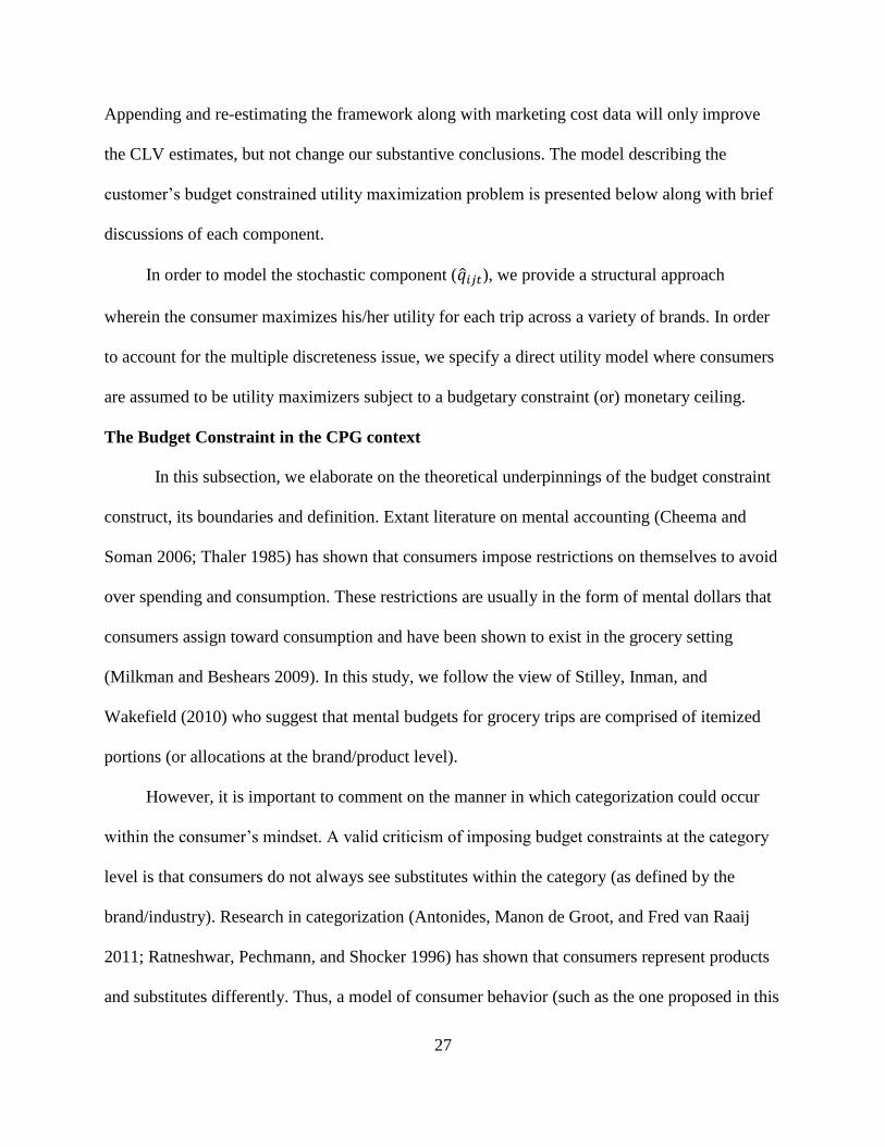
Heterogeneity
Consumers exhibit rich heterogeneity in the frequently purchased goods markets . We
incorporate heterogeneity in the consumer’s inherent brand preference parameter (𝛼𝑖𝑗), the state
dependence coefficient (𝛿𝑖) as well as the baseline budget parameter (𝑦𝑖). We assume that the
above coefficients follow a normal distribution with location parameters specified below,
𝛼𝑖𝑗 ~ 𝑁 (𝛼�̅� , 𝑉𝛼𝑗) ; 𝛿𝑖 ~ 𝑁(𝛿̅ , 𝑉𝛿) ; 휁0𝑖 ~ 𝑁(휁0̅ , 𝑉 0
) (8)
where (𝛼�̅� , 𝑉𝛼𝑗), (𝛿̅ , 𝑉𝛿), and (휁0̅ , 𝑉 0
) represent the population means and variances of the
distribution of 𝛼𝑖𝑗, 𝛿𝑖, and 휁0𝑖 respectively.
Likelihood
Using the assumption of normal errors, equations 5a and 5b can be combined to form the
overall likelihood which is a combination of density (for interior solution) and mass (for corner
solutions). We represent the parameter space as an array “𝛩𝑖” for expositional purposes such that
𝛩𝑖 = {𝛼𝑖𝑗 , 𝛿𝑖, 𝛽, 휁0𝑖 , 휁1−3} and write the likelihood for household ‘i’ as,
Page 34
33
𝐿𝑖(𝛩) = ∫ 𝐿0𝑖(𝛩𝑖)𝐼(𝑞𝑖𝑗𝑡>0) ∙ 𝐿1𝑖(𝛩𝑖)
(1−𝐼(𝑞𝑖𝑗𝑡>0))𝑓(𝛩𝑖)𝑑𝛩𝑖
∞
−∞
= ∫ ∏∏(𝜙(휀𝑖𝑗𝑡) ∙ |𝐽|𝑖𝑗𝑡→𝑞𝑖𝑗𝑡
)𝐼(𝑞𝑖𝑗𝑡>0)
𝐽
𝑗=0
𝑇
𝑡=1
∞
−∞
∙ Φ(휀𝑖𝑗𝑡)(1−𝐼(𝑞𝑖𝑗𝑡>0))
𝑓(𝛩𝑖)𝑑𝛩𝑖
(9)
Where,
𝐼(𝑞𝑖𝑗𝑡 > 0) = { 1 ; 𝑤ℎ𝑒𝑛 𝑞𝑖𝑗𝑡 > 0
0 ; 𝑒𝑙𝑠𝑒
𝜙(. )= pdf of the normal distribution
Φ(. )= truncated normal distribution
|𝐽|𝑖𝑗𝑡→𝑞𝑖𝑗𝑡
= Jacobian of the transformation from the random utility error (휀𝑖𝑗𝑡) to the likelihood
of observed data (𝑞𝑖𝑗𝑡)
𝑓(𝛩𝑖)= heterogeneity distribution of parameter space 𝛩𝑖 with location parameters �̅�, 𝑉𝛩
The Jacobian for our model is given by the first order derivative of the error term with
respect to 𝑞𝑖𝑗𝑡 as given below,
|𝐽|𝑖𝑗𝑡→𝑞𝑖𝑗𝑡
=𝜕휀𝑖𝑗𝑡
𝜕𝑞𝑖𝑗𝑡=
𝜆𝑖𝑃𝑗𝑡
𝑦𝑖𝑡 − ∑ 𝑃𝑗𝑡𝑞𝑖𝑗𝑡𝐽𝑗=1
+𝜆𝑖𝑃𝑗𝑡
2(1 + 𝑞𝑖𝑗𝑡)
(𝑦𝑖𝑡 − ∑ 𝑃𝑗𝑡𝑞𝑖𝑗𝑡𝐽𝑗=1 )
2 (10)
Let N be a collection of all ‘i’ households in the data. Then the overall likelihood for the
data can be given by,
𝐿(𝛩)𝑜𝑣𝑒𝑟𝑎𝑙𝑙 = ∏𝐿𝑖(𝛩)
𝑁
𝑖=1
(11)
Unlike prior work on multiple discreteness (Kim, Allenby, and Rossi 2002), we are
interested in estimating the consumer’s budget constraint in order to assess the ceiling of their
purchase within the category. Thus, we treat the budgetary constraint (𝑦𝑖𝑡) as a parameter and
infer it in the estimation. In the following section, we comment on the theoretical and empirical
identification issues faced when estimating the proposed model.
Page 35
34
Model Identification
Given the structure of our model, it is important to provide some intuition regarding the
identification of the model parameters. The overall utility model (Equation 3) consists of two
main components that need to be estimated in order to achieve our stated objectives, namely, (a)
the baseline utility 𝜓𝑖𝑗𝑡 through its associated hierarchical parameters (𝛼𝑖𝑗, 𝛿𝑖, & 𝛽𝑗) and (b) the
budget constraint 𝑦𝑖𝑡 through its associated hierarchical parameters (휁0𝑖, 휁1, 휁2, & 휁3). Recall that
according to Equation 7, 𝑦𝑖𝑡 is allowed to vary deterministically as a function of a baseline
budget constraint (휁0𝑖) along with exogenous covariates. An identification problem arises when
we attempt to simultaneously evaluate the intrinsic preference at the brand level 𝛼𝑖𝑗, the baseline
budget constraint 휁0𝑖, as well as the Lagrangian 𝜆𝑖. That is, it is possible that one could generate
the same observed data (𝑃𝑗𝑡, and 𝑞𝑖𝑗𝑡) using more than one unique combination of the parameters
(𝛼𝑖𝑗, 휁0𝑖, and 𝜆𝑖). Thus, given the data (which includes price and quantity information at the
customer-brand level), it is not possible to empirically identify all three parameters listed above
(Satomura, Kim, and Allenby 2011). Therefore, we need to fix at least one of these parameters in
order to identify the others jointly. As stated before, our main parameters of interest are the
baseline utilities as well as the budget constraint parameter. In order to uniquely identify 𝛼𝑖𝑗 and
휁0𝑖, we first fix 𝜆𝑖 = 1 and 𝜎2 = 1. The following approach to diagnose the identification
problem in budget constrained utility models has also been used in prior work on multiple
discreteness (see for e.g. Kim, Allenby, and Rossi 2002; Kim, Allenby, and Rossi 2007). We
provide more details on the specific elements in the data that allow us to reliably recover the
parameters as well as theoretical arguments on identification in Appendix A.
The budget constraint (𝑦𝑖𝑡) is modeled in the exponential form in order to constrain it to
positive values (since it is impossible to have negative budgets). Similar to Satomura, Kim, and
Page 36
35
Allenby (2011), we also impose logical ceilings on the budget parameter such that the estimated
value for customer ‘i’ does not exceed the observed maximum purchase value (in dollars) within
the data such that, 𝑦𝑖𝑡 ≥ 𝑚𝑎𝑥(∑ 𝑃𝑗𝑡𝑞𝑖𝑗𝑡𝑗∈𝐽 ).
Estimation
The proposed model was estimated using a hybrid Bayesian Markov chain Monte Carlo
(MCMC) algorithm. The use of Bayesian methods is needed since one of our objectives is to
infer the budget constraint (𝑦𝑖𝑡). The Bayesian approach allows us to create latent variables, use
data augmentation methods and estimate the parameters sequentially. The assumption of normal
errors allows us to break down the estimation process into more efficient Gibbs sampling (from
full conditionals) and Metropolis-Hastings (M-H) sampling methods.
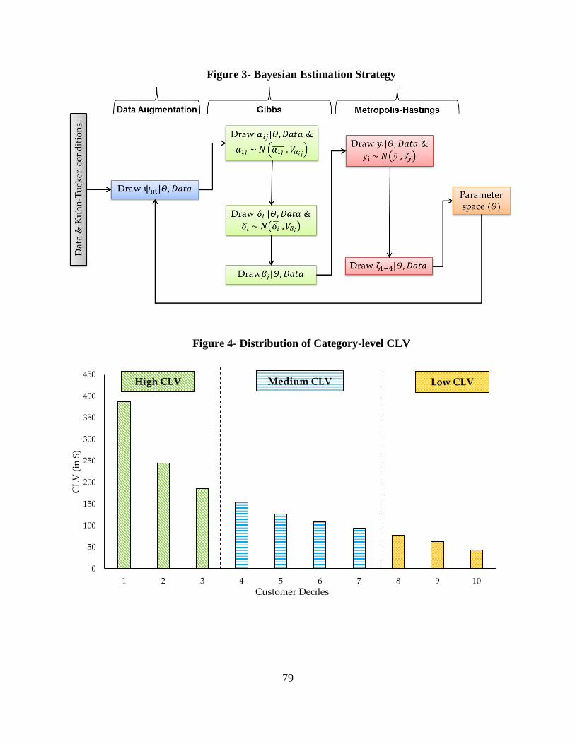
Our estimation process is outlined below (see Figure 3). We first begin by drawing 𝜓𝑖𝑗𝑡
based on whether 𝑞𝑖𝑗𝑡 is equal to or greater than zero. In the case when 𝑞𝑖𝑗𝑡 > 0 (interior
solution), we use the normal distribution to infer 𝜓𝑖𝑗𝑡 and when 𝑞𝑖𝑗𝑡 = 0 (corner solution), we
use the truncated normal distribution to infer 𝜓𝑖𝑗𝑡. Given 𝜓𝑖𝑗𝑡, we now treat the underlying
estimation of 𝛼𝑖𝑗, 𝛿𝑖, and 𝛽𝑗 similar to a multivariate regression with heterogeneous parameters
which can be estimated using Gibbs sampling. The remaining parameters (휁0𝑖, and 휁1-휁4) are
drawn using the M-H algorithm since we cannot derive the full conditional distributions for the
same. We specify the prior distribution on the hyperparameters (𝛼�̅� , 𝑉𝛼𝑗), (𝛿̅ , 𝑉𝛿), and (휁0̅ , 𝑉 0
)
to be non-informative and flat. The prior means were normally distributed and the prior
variances were inverse Wishart distributed. Our overall estimation algorithm is described in
more detail in the Appendix B.
(Insert Figure 3 here)
Page 37
36
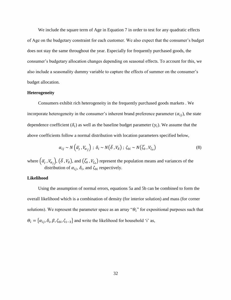
Variable Operationalization
As elucidated in Equation 6, we introduce brand and customer level covariates to explain
variance in the baseline utility equation. We elaborate on the variables used in this study below.
State Dependence: Following prior literature on state dependence in consumer choice , we
include a state dependence term (𝑆𝐷𝑖𝑗𝑡) to track the inertia in the consumer’s purchase pattern. In
the current implementation, we specify state dependence as a dummy variable similar to past
research investigating state dependence in choice modeling (Dubé, Hitsch, and Rossi 2010;
Seetharaman, Ainslie, and Chintagunta 1999). Specifically, if the consumer buys brand ‘j’ during
the previous shopping occasion (t-1), then the state dependence term for that brand is equal to 1.
𝑆𝐷𝑖𝑗𝑡 = 𝐼{𝑞𝑖𝑗𝑡−1 > 0} (12)
The specification in Equation 12 induces a first-order Markov process on choices.
Although this is the specification that is used commonly in empirical research (Dubé, Hitsch, and
Rossi 2010), we note that the above specification is flexible enough to include higher order state
dependence terms as well. It is also important to note that 𝑆𝐷𝑖𝑗𝑡 is brand specific and can take
multiple non-zero values for each purchase occasion, due to the multiple discreteness issue
(where the consumer could have purchased more than one brand at t-1). We refer to 𝛿𝑖 as the
state dependence coefficient that captures the effect of the state dependence term (𝑆𝐷𝑖𝑗𝑡). If 𝛿𝑖 >
0, the model implies that the purchase of a brand reinforces the household’s latent utility for that
brand. By accounting for brand and customer specific intercepts (𝛼𝑖𝑗), we capture the
household’s underlying preferences for brands and also explicitly separate them from the
household’s tendency to be state dependent (𝛿𝑖 > 0).
Page 38
37
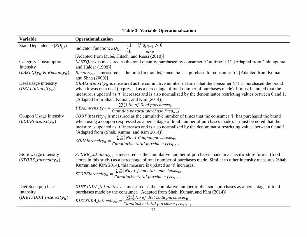
Past purchase behavior: In Equation 6, we also specify 𝑋𝑖𝑡 as a matrix of customer level
variables that could be the drivers of consumer purchase behavior. Table 3 shows the variables
used in this study, their operationalization and expected effects.
(Insert Table 3 here)
In order to capture the consumer’s consumption intensity within the category, we use total
quantity purchased at the previous purchase occasion (𝐿𝐴𝑆𝑇𝑄𝑡𝑦𝑖𝑡) and recency of last purchase
(𝑅𝑒𝑐𝑒𝑛𝑐𝑦𝑖𝑡). These variables are expected to explain the consumer’s category level consumption
patterns by accounting for the incidence of a past purchase as well as the depth of the previous
purchase. Prior research has shown that there exists a negative effect of recency of purchase on
CLV (Kumar and Shah 2009). Within the CPG context, recency will have a negative effect on
quantity purchased. That is, the longer the time since the last purchase, the less likely the
customer is to purchase within the category. For example, consumers who have not made a
category purchase (high values of 𝑅𝑒𝑐𝑒𝑛𝑐𝑦𝑖𝑡) are likely to have churned and thus derive much
lower utility from consuming the brand. In order to capture the effect of the depth of the previous
purchase, we include the lagged values of quantity purchased as a covariate (Chintagunta and
Haldar 1998; Jain and Vilcassim 1991). This variable will also account for observable
differences in consumption among households (such as heavy vs. light users) as well as control
for category consumption levels per household (Jain and Vilcassim 1991).
The general behavioral tendency of a customer to selectively purchase brands that are
offered as ‘deals’ is defined in this study as 𝐷𝐸𝐴𝐿𝑖𝑛𝑡𝑒𝑛𝑠𝑖𝑡𝑦𝑖𝑡. 𝐷𝐸𝐴𝐿𝑖𝑛𝑡𝑒𝑛𝑠𝑖𝑡𝑦𝑖𝑡 indexes the
consumer’s deal usage intensity or the extent to which the consumer purchases brands that are on
deals/features/displays within the store. The role of deals in the CPG setting is not only to
provide monetary savings to the customer but also be able to signal quality . Past research has
Page 39
38
shown that deal usage with regard to national brands (which command higher loyalty) is
associated with higher perceived savings (Ailawadi, Neslin, and Gedenk 2001) and would result
in higher derived utility. Thus, deal usage is expected to have a positive effect on the utility for
national brands. However, the above latent savings are not perceived for store brands (since they
do not command loyalty or high perceived quality). Thus, the high deal intensive consumers
would, in fact derive a lower utility for private labels leading to lower purchase quantities.
Similar to the deal intensity variable, we operationalize 𝐶𝑂𝑈𝑃𝑖𝑛𝑡𝑒𝑛𝑠𝑖𝑡𝑦𝑖𝑡 in order to
capture the coupon usage behavior of consumers. Consumers who are serial coupon users are
likely to purchase only the value of the coupon being offered rather than indulge in cross-buying
or up-buying within the category. Evidence of this behavior was shown in the retailing sector by
Shah, Kumar, and Kim (2014) who study the above phenomenon in the context of promotional
habit strength. Drawing parallels from this research, it is expected that consumers who
consistently use coupons are likely to purchase lesser quantities.
Since the data is from consumers who made purchases from either food or non-food (such
as drug stores) stores, we can study whether consumers who are especially loyal to a specific
kind of store are more/less likely to purchase within the category. Especially important is the fact
that high food store purchase intensity might lead to different effects for different brands
(Ailawadi, Pauwels, and Steenkamp 2008). For example, consumers who are heavy drug store
purchasers may not purchase private labels (possibly due to an availability issue). In this study,
we use 𝑆𝑇𝑂𝑅𝐸_𝑖𝑛𝑡𝑒𝑛𝑠𝑖𝑡𝑦𝑖𝑡 to study whether store format loyalty influences the overall quantity
purchased.
With ever increasing attention being cast on the health impact of foods (especially
carbonated sodas), consumers are moving toward ‘diet’ sodas as an alternative due to their lower
Page 40
39
sugar and calorie content. In fact, recent research by Ma, Ailawadi, and Grewal (2013) shows
that consumers diagnosed with diabetes change their consumption patterns to accommodate a
lower sugar and carbohydrate diet, which in our case translates to a shift from regular to diet
soda. Diet products, thus, are likely to be perceived with a higher utility due to their ‘health’
related advantages. Therefore, higher diet soda consumption in the past (measured as
𝐷𝐼𝐸𝑇𝑆𝑂𝐷𝐴_𝑖𝑛𝑡𝑒𝑛𝑠𝑖𝑡𝑦𝑖𝑡) is likely to lead to a higher consumption in the future. The summary
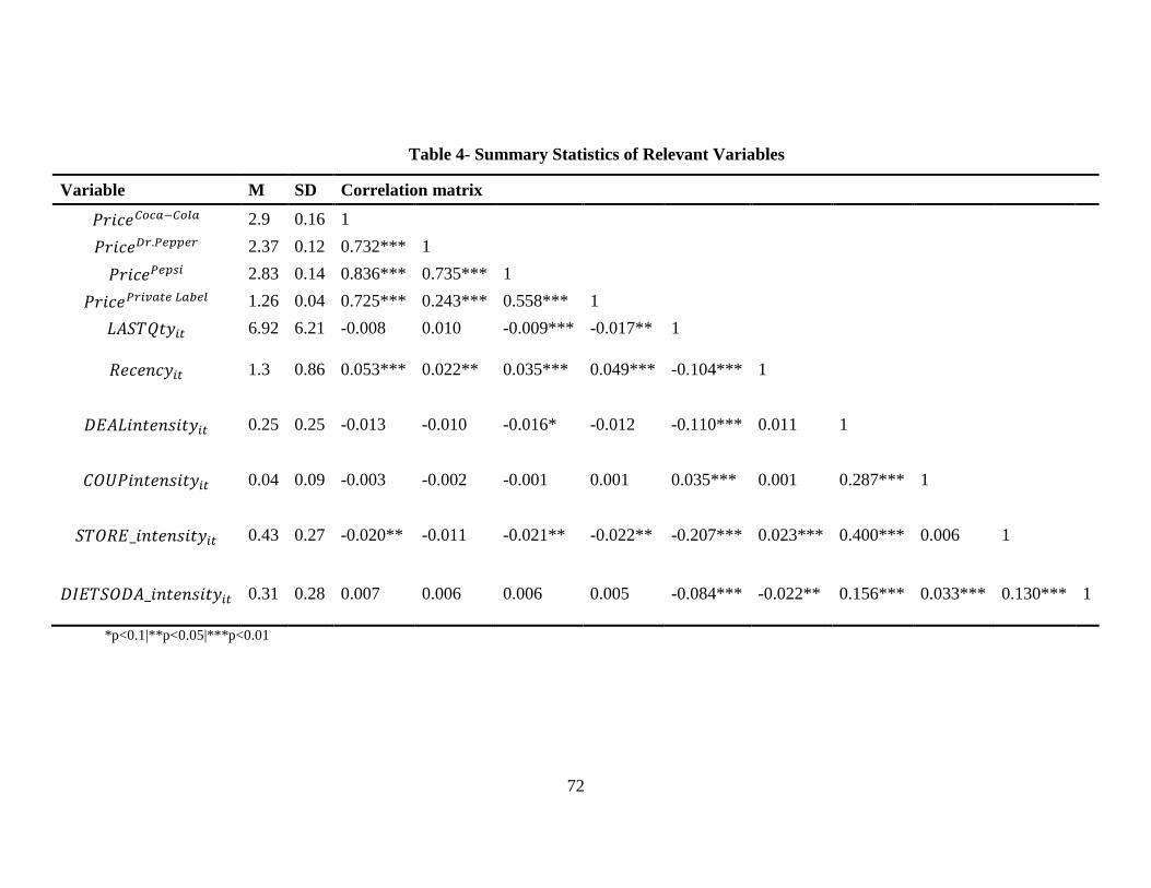
statistics of the data is provided in Table 4.
(Insert Table 4 here)
RESULTS
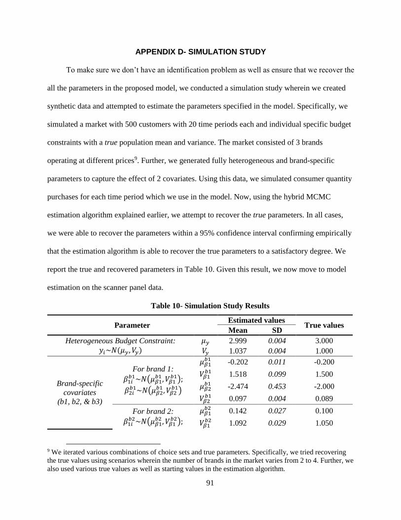
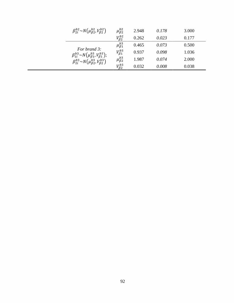
Simulation Study
In order to check the robustness of our model specification and estimation methodology,
we first conducted a simulation study to calibrate the performance of our model. Data was
generated according to the utility specified in Equation 4 assuming a three brand market. We
generated consumption data for 500 consumers each having an observation length of 20 time
periods. All the parameters were well recovered, having the true values within 95% credible
intervals, thus confirming that our estimation method can recover the true parameters and can be
implemented on real transaction data. Please refer to Appendix D for details on the simulation
exercise.
Model Evaluation & Performance
We estimate the proposed model on a randomly selected sample of 500 customers (total
number of transactions= 12,837) from the above described consumer scanner panel data for the
Page 41
40
carbonated beverages category4. We used 20,000 iterations of the Markov chain to generate
parameter estimates, with the first 10,000 discarded as burn-in. In order to assess the
performance of the model, we use the Mean Absolute Deviation (MAD) and Mean Absolute
Percentage Error (MAPE) to assess the predictive accuracy of our model. We rely on MAPE as a
preferred metric to gauge model fit because it is unit-free and easier to interpret. We gauge
model performance for in sample as well as out of sample fit.
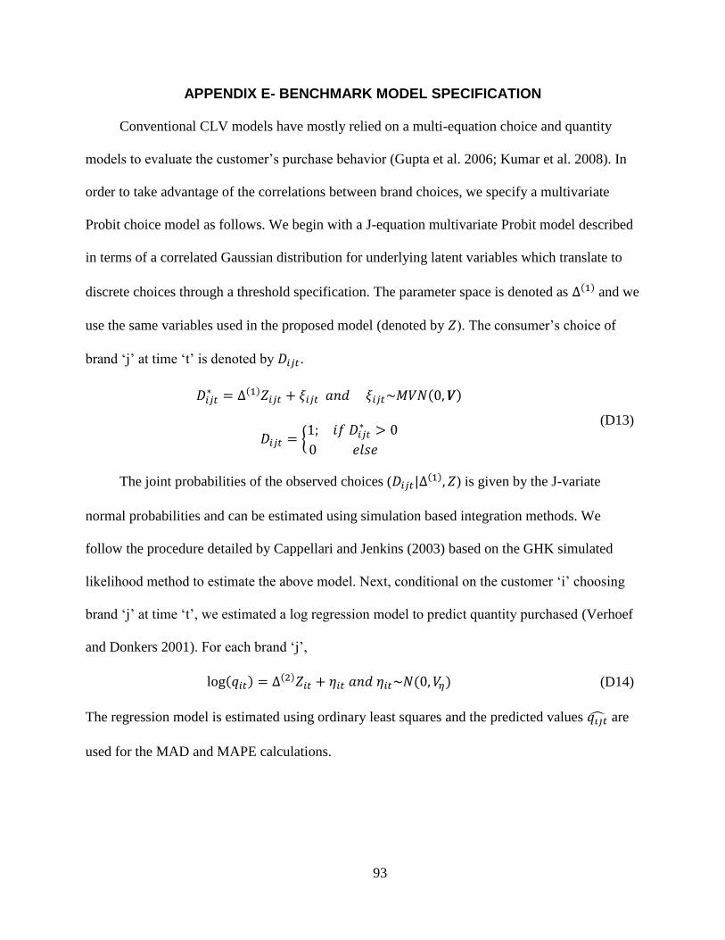
In this section, we compare our modeling approach to a more conventional choice and
quantity modeling approach that is typical for extant CLV models (Gupta et al. 2006).
Specifically, we estimated a multivariate probit choice model using the simulated maximum
likelihood approach to predict customer choice across various brands and subsequently used a
regression model to predict quantity (see Appendix E for model and estimation details). To
assess out of sample fit, we estimated the model using the first 30 months of data and used the
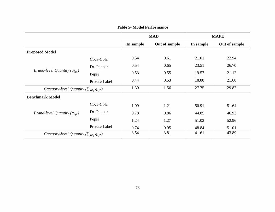
remaining 6 months as hold out. In Table 5, we report in sample and out of sample fit statistics
(MAD and MAPE) for each brand as well as overall category level quantity. As we can see, the
proposed model predicts brand-level quantity purchased (𝑞𝑖𝑗�̂�) quite well, yielding an average
MAPE across brands of 20.74% (in-sample) and 23.09% (out of sample). When considering the
total category quantity purchased, the model performance dips slightly to a MAPE of 27.75% (in
sample) and 29.87% (out of sample). This result is markedly better that the benchmark model
which has an average MAPE of 48.90% (in sample) and 50.64% (out of sample) when predicting
brand level quantities. At the category level, the MAPE is 41.61% (in sample) and 43.89% (out
of sample) which are both worse than the proposed model. The choice then quantity model
4 We repeated the analysis for 3 different samples of 500 customers and arrived at similar estimation
results.
Page 42
41
performs much worse in this case since it involves specifying multiple equations (each
associated with a random utility error) with several parameters. The proposed model is superior
to the conventional CLV modeling approaches as it exploits quantity information within the
choice framework and prevents parameter proliferation (Chintagunta and Nair 2011).
(Insert Table 5 here)
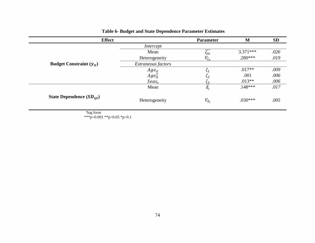
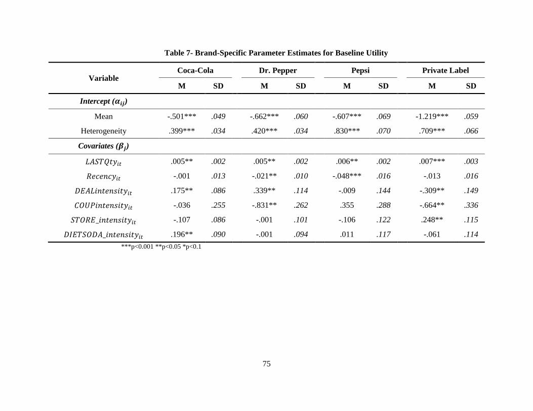
Findings from Model Estimation5
Consumer’s Budget constraint. One of the main modeling issues that we deal with in this study
is the explicit estimation of the consumer’s budget parameter using Bayesian methods. To our
knowledge, this is the first study to estimate the consumer’s budget using transaction data and
use this to calculate CLV. In Table 5, we report the parameter estimates for Equation 10. We find
that the average consumer baseline budget allocation for the carbonated beverages category is
exp(3.371) = $29.40 for a month. Consistent with Du and Kamakura (2008), we find that there is
significant heterogeneity in the budget parameter. This heterogeneity in the consumer’s budget is
important to consider especially in the CPG industry where each consumer/household can have
different thresholds and priorities when allocating a budget toward a particular category. As we
elaborate in the discussion section, CPG companies could potentially build customer profiles for
high budget customers and try to achieve a larger portion of their share of wallet. Further, we
find that the age of the head of the household has a positive effect on the budget. Specifically, as
the consumer ages, the budget allocation toward carbonated beverages also increases. Since the
squared term is not significant, we conclude that the effect is only linear and not quadratic. The
non-significance of the quadratic term could be due to the range of age that we observe in the
5 To establish external validity, we presented our findings to executives from one of the largest firms in
this industry who provided valuable qualitative insights corroborating the results.
Page 43
42
data. Future research could further explore the long-term effect of age on the consumer’s budget
constraint.
(Insert Table 6 here)
Inertia effects: Consistent with Seetharaman, Ainslie, and Chintagunta (1999), we find that there
exists inertia in the marketplace wherein consumers prefer to stick to their past experiences. This
result is consistent with theoretical explanations of routinized response behavior (Assael 1974)
especially in heavily advertised, convenience goods associated with limited informational search
and stronger brand attitudes. Furthermore, we also find that the inertia effect is heterogeneous in
that consumers vary in their levels of inertia (some consumers may be a little bit more variety
seeking that others). By profiling customers who are more/less variety seeking, firms can
identify consumer segments that may have a higher tendency to indulge in brand switching.
Brand-specific effects: Table 7 describes the brand specific parameter estimates for baseline
utility (𝜓𝑖𝑗𝑡). Looking at the heterogeneous intercept term (𝛼𝑖𝑗), we find that consumers are
heterogeneous in their intrinsic preference level for brands in the carbonated beverage category.
Looking at the means of the 𝛼𝑖𝑗 distributions (𝛼𝑖𝑗̅̅ ̅̅ ), we find that the highest preference level is for
Coca-Cola and the least for Private labels. This ordering follows the market share order in the
category where Coca-Cola has the largest market share and Private Labels have the least. As
described previously, heterogeneity (𝑉𝛼𝑖𝑗) is significantly large for this category, a result that was
also demonstrated by Dubé (2004) in the same category. Notably, the heterogeneity term is large
for Pepsi indicating a high variance in intrinsic preferences among Pepsi’s customer base.
(Insert Table 7 here)
Turning to the effect of the covariates, we find that 𝐿𝐴𝑆𝑇𝑄𝑡𝑦𝑖𝑡 positively affects the
consumer’s purchase behavior across all brands. That is, consumers who purchased large
Page 44
43
quantities in the past are likely to do the same in the current period. This result suggests that
consumers do not necessarily take inventory into account when making frequent purchases in the
carbonated beverages category. Further, specific to frequently purchased goods, heavy users
could be developing habits behavior of purchasing that lead to creation of behavioral loyalty.
This result is in line with Venkatesan, Kumar, and Bohling (2007) who also find a positive
relationship between past and current quantity purchase. We also find that the effect of
𝑅𝑒𝑐𝑒𝑛𝑐𝑦𝑖𝑡 is significant and negative for Pepsi and Dr.Pepper while insignificant for the other
brands (even though the sign of the coefficient is consistent). This indicates that consumers who
have not made a purchase in the category in a long time (high recency) have likely churned. The
model suggests that this variable is especially important for Pepsi and Dr.Pepper.
The results suggests that 𝐷𝐸𝐴𝐿𝑖𝑛𝑡𝑒𝑛𝑠𝑖𝑡𝑦𝑖𝑡 is positively associated with Coca-Cola and Dr.
Pepper, but negatively associated with Private Labels. This differential effect of deal usage and
brand preference is supported in the literature. Specifically, Ailawadi, Neslin, and Gedenk (2001)
show that consumers who do not focus on the ‘deal’ aspect of the purchase and therefore make
fewer purchases on deals tend to gravitate toward store brands. Further, consumers who tend to
be quality conscious and deal prone tend to avoid private label brands and gravitate toward
national brands. Turning to the effect of coupon usage behavior, consumers that are serial
coupon users are found to be selective in their purchases and hence, unlikely to exhibit high
purchase behavior. This could be because these consumers only purchase the quantity/value
indicated in the coupon. Similar coupon proneness behavior has been studied recently from a
habitual perspective by Shah, Kumar, and Kim (2014) in a retail setting. Finally, we find that
consumers who purchase frequently at food stores are likely to purchase Private Label brands.
Page 45
44
This could be a factor of the distribution intensity of Private Labels in these stores, thus
increasing product availability.
CLV IN THE CARBONATED BEVERAGES CATEGORY
CLV Measurement
The main objective of this research was to compute the CLV of a customer in the CPG
setting. Using the proposed model, we can now predict the quantity purchased for each brand in
the market (𝑞𝑖𝑗�̂�) using the parameter estimates into the future and substitute the predicted values
in Equation 1 to arrive at the CLV of a customer. First, we hold brand price (𝑃𝑗𝑡) at the mean and
the brand-specific covariates (except 𝐿𝐴𝑆𝑇𝑄𝑡𝑦𝑖𝑡 and 𝑅𝑒𝑐𝑒𝑛𝑐𝑦𝑖𝑡) at the last recorded value for
the CLV prediction, thus making the assumption that the consumer does not change his habits
during the prediction window. Second, for each future period in the prediction window, we
update the 𝐿𝐴𝑆𝑇𝑄𝑡𝑦𝑖𝑡, 𝑅𝑒𝑐𝑒𝑛𝑐𝑦𝑖𝑡 and 𝑆𝐷𝑖𝑗𝑡 variables based on the previous (predicted) values.
Next, using the above generated covariates along with the parameter estimates we generate the
overall utility function (Equation 3) and subsequently maximize this expression to obtain
purchase quantities for each brand. Sufficient logical constraints (𝑞𝑖𝑗�̂� > 0) are applied in the
constrained maximization routine which can be achieved using subroutines in the R software
(e.g. constrOptim, nlminb etc.). This process is repeated for the future time periods (36 months in
our context). We choose a CLV prediction time window of 36 months for the following reasons.
First, given the dynamic environment that CPG firms typically operate, a prediction window of
three years offers a good trade-off between predictive accuracy and horizon when computing
CLV. Second, the choice of a three year window also has roots in managerial decision making
horizons. Prior to computing CLV, we interviewed several executives in one of the firms in the
data to get an understanding of the decision horizons that were generally considered industry
Page 46
45
standards. We learned that due to the dynamic environment in the marketplace, CPG managers
cutoff the decision horizons at 3 years or less, after which marketing allocations are
reconsidered. Finally, in general, the concept of discounting cash flows results in a majority of
the customers’ lifetime value being captured within the three years window (Gupta and Lehmann
2005; Kumar and Shah 2009). For the context of the study, based on the guidance provided by
Nielsen, we use a constant margin value of 0.28 for all the brands. Further, following Yoo,
Hanssens, and Kim (2011) we assume a marketing cost of zero without loss of generality (since
marketing investments in this category are made at the aggregate level and rarely vary across
customers). We do, however acknowledge that each brand would have its own margins and
marketing cost values but due to lack of information, we are forced to make simplifications on
the same.
The above analysis yields a mean CLV of a customer in this category to be $148.69 with a
standard deviation of $101.57. In order to investigate this distribution further, we summarize the
CLV scores of the customers in ten deciles where each decile represents the mean of 10% of the
customers organized in descending order of CLV scores (Figure 4). Similar to prior CLV work,
we find that the bulk of dollars (in the form CLV) are concentrated in the top few deciles. In fact,
the first three deciles constitute almost 55% of the entire profits! This result, though familiar in a
relationship marketing setting is new to the CPG industry and presents further evidence that CPG
brands need to move toward customer centricity rather than relying on aggregate measures of
brand performance (such as market growth, market share, etc.).
(Insert Figure 4 here)
We also compared our proposed CLV segmentation approach to simpler heuristics that are
commonly used by managers. The proposed CLV approach is an improvement over simpler
Page 47
46
naïve heuristics since it accounts for multiple discreteness, unobserved heterogeneity,
competitive effect, variety seeking as well as the consumer’s budget constraint. Although past
literature (Venkatesan and Kumar 2004) has shown that CLV outperforms conventional metrics
and simpler heuristics in various business settings, we assess how well the traditional metrics
match up against the proposed CLV. We focus primarily purchase frequency, consumption level
and monetary value which are commonly used in marketing practice due to their simple
interpretation and implementation. Specifically, we segment the customers based on the above
metrics and compute the mismatch or discordance between the deciles created using simpler
heuristics and the proposed CLV approach. We find that across deciles, there is a significant
mismatch between the metrics. The discordance between deciles was an average of 61.6%
(79.6% for purchase frequency, 56% for total quantity consumed and 49.2% for total revenue)
across metrics. This result further motivates the need for a model based and a predictive method
to assess customer value rather than relying on naïve heuristics that might be easier to interpret
and implement but may lead to suboptimal customer base evaluations.
Studying the Brand’s share of total CLV
Our modeling approach allows us to study not only the customer’s lifetime value for the
entire category, but also the brand level CLV for the category (Equation 1). Using the
distribution of the CLV scores (Figure 4) as basis, we designate customers in Deciles 1, 2 & 3 as
High CLV, Deciles 4, 5, 6, & 7 as Medium CLV and Deciles 8, 9 & 10 as Low CLV. Based on
this classification, we present the brand-level shares of CLV for High, Medium and Low CLV
customers in the carbonated beverages category.
(Insert Figure 5 here)
Page 48
47
Figure 5 presents some interesting results. Although Coca-Cola commands the largest
market share in the carbonated beverages market, surprisingly, in the sample dataset Pepsi tends
to attract a large percentage of the high CLV segment (approximately 41%). This is further
supported through the parameter estimates where we noted that the heterogeneity for inherent
preferences was higher for Pepsi than for Coca-Cola, even though the mean preference level for
Coca-Cola was greater. Further, the majority of medium and low CLV customers are found to be
Coca-Cola customers. We see that Coca-Cola seems to be attracting a majority of the Low CLV
customers, purportedly in an attempt to capture the ‘long tail’. Though this strategy is
commendable, it is still important to capture the high CLV customers since their spending power
(share of wallet-budget) is higher and thus, represent high profit potential. Finally, as expected,
we see that the Private Label brand customers tend to be few and predominantly lower CLV
customers. These customers tend to be value conscious and have little or no brand loyalty
(behavioral and attitudinal) as the quality perceptions for this brand are lesser than the national
brands.
Figure 5 represents an important status quo report of the state of brands in the carbonated
beverages market with respect to CLV. Using the results, managers of each brand will have a
good understanding of the kind of customers that their respective brands have rather than just
using aggregate measures to assess brand performance. In the following section, we conduct two
managerially relevant policy simulations and discuss our findings.
POLICY SIMULATIONS
Simulation Exercise #1: Budget Constraints & CLV
In addition to segmenting the customers into deciles, we are also interested in studying the
relationship between the estimated consumer budget and CLV. High CLV customers seem to
Page 49
48
have high budgetary allocations toward the category and this trend is true for lower CLV deciles
as well. The correlation between CLV and budget is also significant and positive (ρ=0.78;
p<0.001). However, an interesting question is how do consumers react to budget changes?
Further, how does this impact CLV? In fact, recent experimental research by Carlson et al. (2015)
shows that consumers do, in fact change consumption pattern in the presence of shrinking
budgets. Since the proposed modeling framework is structural in nature, we are able to
empirically investigate the budget effects on consumers. That is, we conduct theoretically
grounded policy experiments varying consumer budget constraints and assess the impact on
CLV. Specifically, holding all other effects constant, we attempted to understand the effects of a
20% increase/decrease in budget constraint at the customer level on his/her CLV. Figure 6
describes the results of the policy simulation.
(Insert Figure 6 here)
In Panel 1, we can see that the percentage change in average CLV for an increase in the
budget constraint is lesser than that of a decrease in the budget constraint. This non-linear effect
(concave) of the budget constraint on CLV is important for managers to realize since it has
implications for understanding consumers’ mental accounts for certain categories. Further, from
Panels 2-4, we can see that the effects are different depending on the type of customer.
Specifically, we can see that high CLV customers’ future profitability is least affected by
changes in the budget constraint. However, low CLV customers tend to be more sensitive to
budget constraint changes. Thus, brands that tend to attract low CLV customers need to be aware
of the conditions or situations (such as recessionary trends) that could influence the consumer’s
mental accounting process and, eventually the budget constraint.
Page 50
49
Simulation Exercise #2: Pricing & Consumption
One of the key firm action variables that managers use to improve brand performance in
the CPG setting is price. Although we do not specifically estimate a price coefficient in the
model, we can easily assess own and cross price effects through policy simulations. Further, in
our model, the budget constraint parameter acts as a ceiling and helps us identify competition
between brands. That is, customers with large budgets are likely to be more price inelastic since
for price increases they are more likely to absorb the extra cost of consumption as long as their
budget slack is high. However, this may not be the case for customers who have a lower budget
constraint. In such a case, the limiting nature of the budget constraint forces customers to
reevaluate and adjust their consumption across brands in reaction to a price increase. Given this,
it is important for managers to assess which customers are more/less elastic and where the brand
switching will occur. If Coca-Cola increases its price, which customers are more likely to
purchase other brands and which brands are considered as close substitutes in this market?
Finally, do price increases and decreases lead to symmetric responses among consumers? We
attempt to answer these key questions through a policy simulation exercise where we simulate
consumer responses for variations in price.
We generate two scenarios, wherein the focal brand’s price increases by 10% and price
decreases by 10% while maintaining all other covariates and other brand prices constant. Using
the estimated parameters (𝛩) along with the new price information, we simulate the consumer’s
quantity purchases (𝑞𝑖𝑗�̂�). In Table 8 and Table 9, we report the findings from this policy
simulation.
(Insert Table 8 and Table 9 here)
Page 51
50
In Table 8, we report the effects of a 10% increase (decrease) in focal brand’s price on the
percentage change in average quantity demanded. First, we can see that the direction of the price
elasticity is negative for price increases and positive for decreases. However, the magnitude of
the effect across brands is not symmetric. The absolute value of the effect of a 10% decrease in
price is greater than the corresponding increase in price. This nonlinearity in price elasticity is
consistent across brands. Second, looking at the magnitude of the own effects (diagonals
elements in Table 8), we see that private labels exhibit the highest price elasticity with Coca-
Cola, Pepsi and Dr. Pepper following. Using this result, managers can assess how CPG
customers react to changes in price. Further, looking at the cross price effects, we find that
changes to Coca-Cola prices influence Pepsi and vice versa. This indicates that Pepsi and Coca-
Cola are closely competing with one another and price is a key differentiator. This result is
further substantiated in model free analyses (Figure 1).
While the above analyses gives us an understanding of the average effects of price on
brands, a key element of this study is the issue of heterogeneity. While aggregate data analysis
techniques commonly used by CPG brands can assess price elasticity at the aggregate level, it is
important to address heterogeneity in this construct. Specifically, do CLV segments react
differently to price changes? To illustrate this, we conduct a policy simulation wherein we varied
Coca-Cola’s price by 10% and assessed its corresponding effect on customers in high, medium
and low CLV segments (Table 9)6. We find that the high CLV segment (-7.28% for price
increase and 8.93% for price decrease) and the low CLV segments (-10.14% for price increase
and 12.39% for price decrease) are indeed very different in their responses to price changes.
High CLV customers are less sensitive to price than low CLV customers. This is likely because
6 The policy simulations for Dr. Pepper, Pepsi and Private Labels are presented in Appendix F.
Page 52
51
of the higher budget constraint for high CLV customers and the lower budget constraint for low
CLV customers. This result is important for CPG managers when assessing pricing changes as
they can now evaluate the heterogeneous effect of price on specific CLV segments.
DISCUSSION
CLV/CE gives the firm a long-term, forward looking, profitability oriented view of the
customer base. However, academic work to date has been relatively silent in applying CLV in
the CPG context. In this paper, we attempt to address this gap by proposing a structural approach
to measuring the CLV of a CPG customer while accounting for the nuances and challenges of
model building in the CPG context. We believe that this research addresses some important
issues in its attempt to bridge the gap between customer base evaluation (CLV metrics) and the
CPG context. One of the main objectives of the Marketing Accountability Standards Board
(MASB) is to enhance the role of marketing in the board room. While several industries (with a
large focus on relationship marketing) have adopted CLV and are able to enhance the role of
marketing in the boardroom, CPG firms tend to lag behind. By relying on short term value
metrics (such as market share, sales etc.), CPG managers find it difficult to establish a long-term
profitability focus for marketing strategy. We attempt to resolve this issue in this study by
proposing a structural approach to modeling the CLV of a CPG customer. We implement our
modeling framework on transaction data in the carbonated beverages industry and develop
insights for the same. Some findings and potential managerial implications of this research are
discussed below.
One of the unique aspects of this study is that, in addition to measuring CLV, we also
explicitly infer the consumer’s budget allocations (through a Bayesian approach) toward his/her
mental category and also draw associations between budgetary allocations and CLV. Given our
Page 53
52
model specification, we are able to measure not only overall CLV for the category, but also CLV
at the brand level. CPG managers can make use of this information to understand (a) where their
firm stands with regard to future customer profitability and (b) how to move up the profitability
ladder (to attract high CLV customers).
Specific to the carbonated beverages market, we outline customer behaviors that influence
purchase patterns. We find that there exists a significant level of inertia (positive state
dependence) among consumers of carbonated beverages. However, this effect is heterogeneous
such that consumers have varying levels of inertia in their purchase patterns. We also find that,
on the average, Coca-Cola is the most preferred brand while Private Labels are least preferred.
This is congruent with the market shares within the market. While as expected, this preference is
heterogeneous, we find that the heterogeneity parameter is largest for Pepsi. That is, even though
the average preference for Pepsi is not very high, there are some consumers who are extremely
loyal to the brand. This is evident in our CLV computation as well where we see that about 40%
of the CLV share of the High CLV segment within our random sample belongs to Pepsi. Further,
from our analysis, it is clear that Coca-Cola customers are not necessarily the most behaviorally
loyal. We identify specific past behavior variables that affect the future purchase pattern of the
customer and show that these effects are different for different brands. Specifically, we note that
depending on the focal brand (Coca-Cola, Pepsi, Dr. Pepper, or Private Labels) the drivers of
CLV are different. For example, customer deal usage intensity effect is positive for Coca-Cola
and Dr. Pepper, but negative for the Private Label. Such outcomes are very useful for managers
of CPG brands who can now allocate marketing spend accordingly. Additionally, we note that
the proposed framework is flexible enough to be estimated at the sub-brand (e.g. Diet Coke,
Page 54
53
Regular Coke etc.) and subcategory levels depending on the managerial need. This flexibility
adds to the practical applicability of the proposed framework.
Finally, since our model is structural in nature we are able to conduct theoretically
grounded policy simulations (what-if scenarios), a departure from reduced form modeling
approaches that are common in CLV literature. We conduct managerially relevant policy
simulations. Specifically, we show that the budget constraint and prices asymmetrically affect
consumers. A 20% increase in the budget constraint leads to an average of 1.99% increase in
CLV while the same percentage decrease in the budget constraint leads to a 2.89% decrease in
CLV. We show that this effect too, is heterogeneous. High CLV customers are less volatile (with
respect to changes to the budget constraint) in comparison to lower CLV customers. We see a
similar asymmetric result for price changes suggesting nonlinear price elasticity. Further, we
show that Coca-Cola and Pepsi (the market leaders) are in close competition with regard to price
while Dr. Pepper seems to be least elastic.
This research also has implications for retailers (such as Kroger, Target, etc.) and market
research companies (such as A.C. Nielsen) who collect longitudinal transaction data on
customers. Using the proposed CLV modeling approach, retailers can make product assortment
decisions based on long-term customer profitability as well as create leverage down the supply
chain. Further, since this model is flexible to account for multiple categories, CLV can also be
computed at the retailer level which has implications for marketing strategy at the retailer level
as well.
IMPLEMENTING CLV IN THE CPG CONTEXT
It is no secret that firms have started to treat customers differentially. While the world of
marketing is moving fast from a product centric to a customer centric paradigm, where the onus
Page 55
54
is to gain a 360-degree view of the customer the moment he/she walks into the store. Especially
with the growth of the Internet of Things7 concept, where appliances, products, brands and
consumers are interconnected closely (Atzori, Iera, and Morabito 2010), the need to customize
and individually market to consumers is paramount. In such a marketplace reality, Consumer
Packaged Goods (CPG) industries are mostly being left behind due to several reasons. Being
largely product centric in the past and mostly relying on flow based aggregate metrics of
performance, CPG firms need to move to a customer centric CLV based paradigm. However it is
important to comment on the key issues faced by CPG firms when attempting to assess CLV.
Specifically, managers need to establish vital mechanisms that enable the collection and
utilization of disaggregate data.
CPG manufacturers (such as Unilever, Proctor & Gamble, etc.) rarely have access to
individual customer transaction data over a long period of time. This is because the actual data
collection happens outside the control of the manufacturer. The data collection (at Point-Of-Sale
(POS) systems) happens at the retailer’s premises. Thus the ownership of the customer
transaction data resides with the retailer. The retailer may or may not want to this disaggregate
data since it also represents a competitive advantage to the retailer (due to store labels etc.). To
overcome this problem, manufacturers have two broad options, (a) Collaborate closely with the
retailer, or (b) purchase data from third party firms. The first option involves a deep
collaboration and negotiation with the retailer and possibly, entering into a contractual
relationship with the retailer. Some opportunities regarding this have been outlined in the supply
chain management literature (for e.g. Sari 2008). The second option for CPG manufacturers is to
7 Wasik, Bill (2013), "In the programmable world, all our objects will act as one," [available at
http://www.wired.com/2013/05/internet-of-things-2/].
Page 56
55
purchase scanner/panel data from syndicated sources such as A.C. Nielsen or IRI. This method
of purchasing secondary panel data is commonly used in marketing research as well as in
marketing practice. Several research papers in marketing have leveraged this data to develop
insights on the effect of marketing mix on customer behavior (for e.g. Guadagni and Little 1983;
Kamakura and Russell 1993). In the absence of advanced forms of retailer-manufacturer
collaboration (such as Vendor Managed Inventory (VMI) or Collaborative Planning, Forecasting
and Replenishment (CPFR) systems), our recommendation to manufacturers is to address the
data void using syndicated sources.
The adoption of CLV opens the door to proactive customer management and marketing
decisions. In following paragraphs, we outline a few key strategic implications of implementing
CLV in the CPG context.
Embracing the Customer-centricity Paradigm
CLV has been applied and its benefits have been showcased in several industries and
business settings. Some examples of CLV implementations in various industries include
insurance (Verhoef and Donkers 2001), catalog mailing (Petersen and Kumar 2015), B2B Hi-
tech (Kumar et al. 2008), airlines (Rust, Lemon, and Zeithaml 2004), internet retail (Fader,
Hardie, and Lee 2005), automobile (Yoo and Hanssens 2005), telecommunications (Kumar,
Petersen, and Leone 2013), financial services (Shah et al. 2012). A common theme among the
above implementations is that past implementations of CLV have been mostly on ‘relationship’
driven business settings. That is, the adoption of CLV and customer centric concepts have been
restricted to industries which have been heavily focused toward building customer relationships.
A glaring gap in the above is that the CPG industry is yet to adopt the customer centric concept.
Even today, most CPG managers rely on flow-based and product centric metrics to evaluate
Page 57
56
marketing effectiveness. While this has worked in the past, it is no longer sustainable. By relying
on flow based aggregate measures (such as sales, revenue, market share, etc.) CPG managers are
leaving the customer at the door! For example, when studying the effectiveness of a promotional
campaign, managers would likely state that there is a sales bump during the promotional period
thereby concluding that the promotional campaign has a positive effect on sales. But where is the
sales coming from? Which customers are really purchasing the product? Could it be that the
promotion only attracted deal prone unprofitable customers? Further, did the promotional
campaign help the firm cultivate behavioral loyalty (measured as CLV)? Answers to these
questions are not obvious using aggregate metrics.
Secondly, flow based metrics that are currently used in CPG industries are very sensitive to
extraneous shocks (such as small changes in macroeconomics). The volatility that arises due to
this makes marketing decision making error prone and inaccurate since managers are unable to
assess why a certain phenomenon occurs. Business performance in CPG markets is fast moving
and volatile, especially in the presence of heavy promotional spending, thereby leading to short
run myopic marketing decisions which are based on reaction rather than with strategic focus
(Hanssens and Dekimpe 2008; Yoo, Hanssens, and Kim 2011). In such environments, it is
difficult to assess whether a brand is doing well or not. CLV (or its aggregated counterpart,
Customer equity (CE)) presents stability based on consumer behavior which is long term focused
and forward looking in nature.
In a digitally connected world, where consumers engage with each other as well as the
brand in real time, the customer centric paradigm (especially in the CPG setting) is no longer a
competitive advantage but a necessity. CPG firms are investing heavily in innovations in CRM
that would move them closer to a CLV based approach to decision making (e.g. Kimberly-
Page 58
57
Clark’s Huggies brand8). By analyzing customer level transaction data (obtained through scanner
panel studies), managers at Kimberly-Clark were able to not only quantify the dollar value of
specific consumer segments, but also chart the lifecycle of the customer relationships. As a
result, Kimberly-Clark was able to garner a clearer picture of its target market as well as the
profitable opportunities (consumers) that exist in the marketplace.
Framework to Manage Customer Relationships
A CLV based marketing approach allows the firm to view the customer as an asset
(Srivastava, Shervani, and Fahey 1998) and assess the impact of marketing spend on customer
level assets. CLV adoption fits very closely within the customer centricity paradigm where the
core philosophy is to ‘serve the customer’ and achieve ‘customer profitability’. Couched within
customer centricity are concepts central to marketing such as the need to increase focus on
customer satisfaction (Oliver 1999), customer service (Zeithaml, Berry, and Parasuraman 1993),
customer loyalty (Reinartz and Kumar 2002), quality perceptions (Rust, Moorman, and Dickson
2002) etc. CLV represents a path to achieving improvements in the above critical marketing
metrics while maintaining high levels of profitability. In the recent years, CLV, its applications
to various industries have received attention not only among researchers but in practitioner-
focused books as well (for e.g. Bejou, Keiningham, and Aksoy 2012; Kumar 2014).
The CLV metric opens the door for managers to differentially allocate marketing dollars to
specific types of customers (or) segments of customers based on their profitability. This
capability has spurned a great deal of innovations in building marketing strategy to maximize
8 Nielsen (2011), "Nielsen Insights in Action: Determining Consumer Lifetime Value," (accessed April
24, 2015), [available at
http://www.nielsen.com/content/dam/corporate/us/en/public%20factsheets/Case%20Studies/CaseStudy-
KimberlyClark-ROI.pdf].
Page 59
58
profitability through CLV. By adopting CLV based marketing strategies, marketers can now not
only identify their most valuable customers, but also manage the entire customer relationship
from acquisition to retention. Some examples of the strategic implementations of include
managing acquisition and retention (Reinartz, Thomas, and Kumar 2005), customer
churn/defection (Neslin et al. 2006), product return behavior (Petersen and Kumar 2015) to name
a few. For a detailed review of the customer management strategies that could be implemented
through CLV, please refer to the ‘Wheel of Fortune’ strategies by Kumar (2009). Further, CLV
can be flexibly used for making resource allocation decisions in order to achieve financial
performance. Upon implementing a CLV based paradigm, firms have the capability to vary
marketing actions and spend in order to arrive at an optimal marketing mix. Venkatesan (2015)
guides managers in this direction by providing a five step process to optimal resource allocation
using CLV. Critically important to the success of the above is the adoption of CLV.
Linking Marketing to Firm Value
In today’s marketing world, it is not only important to show growth in marketing metrics
(such as quality perceptions, satisfaction levels etc.), but also in financial metrics. In fact, Welch
(2004) raises alarm that marketers are slowly losing ground in the boardroom since firms and
shareholders are demanding that marketing be linked with firm financials. Taking this challenge
head on, researchers have shown that CLV is one of the best paths to creating firm value.
Adopting a CLV or Customer Equity (CE) based metric has been shown to have extremely high
financial benefits (Bolton 2004; Gupta and Zeithaml 2006; Kumar and Shah 2009). In fact,
Gupta and Zeithaml (2006), in their review article on the link between customer metrics and firm
performance, make a generalization (based on several years of empirical research) that
“Marketing decisions based on observed customer metrics, such as CLV, improve a firm’s
Page 60
59
financial performance”. Customer relationships need to viewed as investment decisions and
therefore, customers need to be viewed as assets who generate revenue. CLV based metrics not
only improve shareholder value by increasing cash flow, but also by reducing retention and
switching costs (Stahl, Matzler, and Hinterhuber 2003). Further, a well-managed CLV paradigm
has the capability to accelerate cash flows (through cross selling etc.), reducing cash flow
volatility & vulnerabilities (through the constancy of demand from loyal customers) and increase
the residual value of the firm (through quality, trust, commitment and reputation). These
advantages make customer centric firm attractive to investors who value the above
characteristics. To this end, past research encourages firms to report CLV/CE based measures in
their financial reports. Specifically, Wiesel, Skiera, and Villanueva (2008) recommend firms to
report CLV to investors since such reports align customer management with corporate goals and
investor perspectives. Customer Lifetime Value (CLV) signals the health of a firm and therefore,
improves investor perceptions in Wall Street.
In conclusion, CLV is a metric that is gaining wide acceptance in the marketplace due to
its enormous strategic, operational and financial benefits. Therefore, CPG firms would be
heavily benefitted by involving Customer Lifetime Value (CLV) in their decision making to
ensure future growth and sustainable competitive advantage.
LIMITATIONS AND OPPORTUNITIES FOR FUTURE RESEARCH
We believe that this research opens several interesting avenues for further research (such
as multi-category CLV, uncovering factors that influence the consumer’s budget etc.) and also
help CPG firms move further down the path toward building strategies to maximize customer
level profits. Our proposed empirical illustration is focused toward single category purchases
while considering CLV at the manufacturer level. However, an interesting avenue to explore
Page 61
60
could be to expand the analysis to consider a basket of goods such that we can study CLV from a
retailer’s perspective. Also interesting is the exploration of cross-category effects and the
retailer’s decision within the CLV framework. That is, as Shankar and Kannan (2014) elaborate,
retailers need to know which category needs to be stocked more and when should bundling be
marketed by the retailer. A retailer level CLV model accounting for cross-category dependencies
could be a logical next step in expanding the CLV concept to grocery purchases and also help
design profitable pricing strategies. In our analyses, due to lack of marketing data, we are unable
to include marketing cost information within the CLV computation. Possibly, the use of
cooperative databases that track marketing information (Liu, Pancras, and Houtz 2014) could
mitigate this issue and provide more robust CLV estimates in this industry.
While the proposed model is estimated at the brand level, it is conceivable that one could
implement the model on more disaggregated choice sets (such as brand-sizes) rather than just
brands (Fader and Hardie 1996; Pancras 2011). Within our data, as we do not observe enough
variation in the consumption patterns across brand-size alternatives, we are unable to estimate
such a model without having to face increased complexities and identification issues in the
model. We acknowledge that inclusion of the size information (especially within the choice sets)
could increase the efficiency of the CLV model and leave the formal investigation of this issue to
future research. An issue that could arise within the proposed framework is that there could be
correlated unobservables (such as extraneous shocks) that might influence the covariates as well
as the consumption patterns. In our model, we are unable to control for this because we allow for
the budget parameter to vary across time only deterministically and not stochastically. Thus, we
would not be able to assess (or observe) stochastic shocks to the system that might influence the
consumption. However, a formal dynamic model with stochastically varying budgets (with
Page 62
61
serially correlated errors) would significantly complicate the estimation process and lead to
empirical identification issues due to the parameter proliferation problem. Future research could
specify a dynamic model of consumer budgeting behavior and incorporate this within the CLV
framework. As an extension, future research could also explicitly study the drivers of consumer
budgeting behavior in the CPG setting. Further, an extension of this research could include
complementarities across and within the category to increase efficiency of the estimation and
gather insights.
Page 63
62
REFERENCES
Ailawadi, Kusum L., Scott A. Neslin, and Karen Gedenk (2001), "Pursuing the Value-Conscious
Consumer: Store Brands Versus National Brand Promotions," Journal of Marketing, 65 (1),
71-89.
Ailawadi, Kusum L., Koen Pauwels, and Jan-Benedict E. M. Steenkamp (2008), "Private-Label
Use and Store Loyalty," Journal of Marketing, 72 (6), 19-30.
Albert, James H. and Siddhartha Chib (1993), "Bayesian Analysis of Binary and Polychotomous
Response Data," Journal of the American Statistical Association, 88 (422), 669-79.
Allenby, G. M. and Peter E. Rossi (1998), "Marketing models of consumer heterogeneity,"
Journal of econometrics, 89 (1-2), 57.
Allender, William J., Timothy J. Richards, Sungho Park, and Stephen F. Hamilton (2013),
"Demand for Variety Under Costly Consumer Search: A Multiple-Discrete/Continuous
Approach," Working Paper.
Antonides, Gerrit, I. Manon de Groot, and W. Fred van Raaij (2011), "Mental budgeting and the
management of household finance," Journal of Economic Psychology, 32 (4), 546-55.
Assael, Henry (1974), "Product classification and the theory of consumer behavior," Journal of
the Academy of Marketing Science, 2 (4), 539-52.
Atzori, Luigi, Antonio Iera, and Giacomo Morabito (2010), "The Internet of Things: A survey,"
Computer Networks, 54 (15), 2787-805.
Bejou, David, Timothy L. Keiningham, and Lerzan Aksoy (2012), Customer Lifetime Value:
Reshaping the Way We Manage to Maximize Profits. New York, NY: Routledge.
Bell, David R., Jeongwen Chiang, and V. Padmanabhan (1999), "The Decomposition of
Promotional Response: An Empirical Generalization," Marketing Science, 18 (4), 504-26.
Bhat, Chandra (2005), "A multiple discrete–continuous extreme value model: formulation and
application to discretionary time-use decisions," Transportation research. Part B:
methodological, 39 (8), 679-707.
Bolton, Ruth N. (2004), "Linking Marketing to Financial Performance and Firm Value," Journal
of Marketing, 68 (4), 73-75.
Borle, Sharad, Siddharth S. Singh, and Dipak C. Jain (2008), "Customer Lifetime Value
Measurement," Management Science, 54 (1), 100-12.
Cappellari, Lorenzo and Stephen P Jenkins (2003), "Multivariate probit regression using
simulated maximum likelihood," The Stata Journal, 3 (3), 278-94.
Page 64
63
Carlson, Kurt A., Jared Wolfe, Simon J. Blanchard, Joel C. Huber, and Dan Ariely (2015), "The
Budget Contraction Effect: How Contracting Budgets Lead to Less Varied Choice," Journal
of Marketing Research, 52 (3), 337-48.
Carpenter, Gregory S. and Donald R. Lehmann (1985), "A Model of Marketing Mix, Brand
Switching, and Competition," Journal of Marketing Research, 22 (3), 318-29.
Cheema, Amar and Dilip Soman (2006), "Malleable Mental Accounting: The Effect of
Flexibility on the Justification of Attractive Spending and Consumption Decisions," Journal
of Consumer Psychology, 16 (1), 33-44.
Cheng, Ching-Hsue and You-Shyang Chen (2009), "Classifying the segmentation of customer
value via RFM model and RS theory," Expert Systems with Applications, 36 (3, Part 1), 4176-
84.
Chib, Siddhartha (1992), "Bayes inference in the Tobit censored regression model," Journal of
Econometrics, 51 (1–2), 79-99.
Chintagunta, Pradeep K. and Sudeep Haldar (1998), "Investigating Purchase Timing Behavior in
Two Related Product Categories," Journal of Marketing Research, 35 (1), 43-53.
Chintagunta, Pradeep K. and Harikesh S. Nair (2011), "Structural Workshop Paper—Discrete-
Choice Models of Consumer Demand in Marketing," Marketing Science, 30 (6), 977-96.
Du, Rex Y. and Wagner A. Kamakura (2008), "Where Did All That Money Go? Understanding
How Consumers Allocate Their Consumption Budget," Journal of Marketing, 72 (6), 109-31.
Dubé, Jean-Pierre (2004), "Multiple Discreteness and Product Differentiation: Demand for
Carbonated Soft Drinks," Marketing Science, 23 (1), 66-81.
Dubé, Jean-Pierre, Günter J. Hitsch, and Peter E. Rossi (2010), "State dependence and alternative
explanations for consumer inertia," The RAND Journal of Economics, 41 (3), 417-45.
Erdem, Tülin and Michael P. Keane (1996), "Decision-Making under Uncertainty: Capturing
Dynamic Brand Choice Processes in Turbulent Consumer Goods Markets," Marketing
Science, 15 (1), 1-20.
Fader, Peter S, Bruce GS Hardie, and Ka Lok Lee (2005), "RFM and CLV: Using iso-value
curves for customer base analysis," Journal of Marketing Research, 415-30.
Fader, Peter S. and Bruce G. S. Hardie (1996), "Modeling Consumer Choice among SKUs,"
Journal of Marketing Research, 33 (4), 442-52.
Fader, Peter S., Bruce G. S. Hardie, and Jen Shang (2010), "Customer-Base Analysis in a
Discrete-Time Noncontractual Setting," Marketing Science, 29 (6), 1086-108.
Page 65
64
Gilboa, Itzhak, Andrew Postlewaite, and David Schmeidler (2010), "The Complexity of the
Consumer Problem and Mental Accounting," Working Paper.
Gordon, Brett R., Avi Goldfarb, and Yang Li (2013), "Does Price Elasticity Vary with Economic
Growth? A Cross-Category Analysis," Journal of Marketing Research, 50 (1), 4-23.
Guadagni, Peter M. and John D. C. Little (1983), "A Logit Model of Brand Choice Calibrated on
Scanner Data," Marketing Science, 2 (3), 203-38.
Gupta, Sunil, Dominique Hanssens, Bruce Hardie, Wiliam Kahn, V. Kumar, Nathaniel Lin,
Nalini Ravishanker, and S. Sriram (2006), "Modeling Customer Lifetime Value," Journal of
Service Research, 9 (2), 139-55.
Gupta, Sunil and Donald R. Lehmann (2005), Managing Customers as Investments: The
Strategic Value of Customers in the Long Run. Upper Saddle River, NJ 07458: Wharton
School Publishing.
Gupta, Sunil and Valarie Zeithaml (2006), "Customer Metrics and Their Impact on Financial
Performance," Marketing Science, 25 (6), 718-39.
Hanssens, Dominique and Marnik Dekimpe (2008), "Models for the Financial Performance
Effects of Marketing," in Handbook of Marketing Decision Models, Berend Wierenga, ed.
New York, NY: Springer Science+Business Media, LLC.
Hastings, Justine S. and Jesse M. Shapiro (2013), "Fungibility and Consumer Choice: Evidence
from Commodity Price Shocks*," Quarterly Journal of Economics, 128 (4), 1449-98.
Heath, Chip and Jack B. Soll (1996), "Mental Budgeting and Consumer Decisions," Journal of
Consumer Research, 23 (1), 40-52.
Jain, Dipak C. and Naufel J. Vilcassim (1991), "Investigating Household Purchase Timing
Decisions: A Conditional Hazard Function Approach," Marketing Science, 10 (1), 1.
Kamakura, Wagner A. and Gary J. Russell (1993), "Measuring brand value with scanner data,"
International Journal of Research in Marketing, 10 (1), 9-22.
Keane, Timothy J. and Paul Wang (1995), "Applications for the lifetime value model in modern
newspaper publishing," Journal of Direct Marketing, 9 (2), 59-66.
Kim, Jaehwan, Greg M. Allenby, and Peter E. Rossi (2002), "Modeling Consumer Demand for
Variety," Marketing Science, 21 (3), 229-50.
_____ (2007), "Product attributes and models of multiple discreteness," Journal of
Econometrics, 138 (1), 208-30.
Page 66
65
Kumar, V. (2009), Managing customers for profit: strategies to increase profits and build loyalty:
Wharton School Publishing, Upper Saddle River, NJ 07458.
_____ (2014), Profitable Customer Engagement: Concept, Metrics and Strategies. New Delhi,
India: SAGE Publications India Pvt Ltd.
Kumar, V. and Anita (Man) Luo (2008), "Integrating Purchase Timing, Choice and Quantity
Decisions Models: A Review of Model Specifications, Estimations and Applications," in
Review of Marketing Research, Naresh K. Malhotra, ed.: Emerald Group Publishing Limited.
Kumar, V., J. Andrew Petersen, and Robert P. Leone (2013), "Defining, Measuring, and
Managing Business Reference Value," Journal of Marketing, 77 (1), 68-86.
Kumar, V. and Denish Shah (2009), "Expanding the Role of Marketing: From Customer Equity
to Market Capitalization," Journal of Marketing, 73 (6), 119.
Kumar, V., Rajkumar Venkatesan, Tim Bohling, and Denise Beckmann (2008), "The Power of
CLV: Managing Customer Lifetime Value at IBM," Marketing Science, 27 (4), 585-99.
Liu, Hongju, Joseph Pancras, and Malcolm Houtz (2014), "Managing Customer Acquisition
Risk Using Co-Operative Databases," Working Paper.
Ma, Yu, Kusum L. Ailawadi, and Dhruv Grewal (2013), "Soda Versus Cereal and Sugar Versus
Fat: Drivers of Healthful Food Intake and the Impact of Diabetes Diagnosis," Journal of
Marketing, 77 (3), 101-20.
Manchanda, Puneet, Asim Ansari, and Sunil Gupta (1999), "The "Shopping Basket": A Model
for Multicategory Purchase Incidence Decisions," Marketing Science, 18 (2), 95-114.
McCulloch, Robert and Peter E. Rossi (1994), "An exact likelihood analysis of the multinomial
probit model," Journal of Econometrics, 64 (1–2), 207-40.
Milkman, Katherine L. and John Beshears (2009), "Mental accounting and small windfalls:
Evidence from an online grocer," Journal of Economic Behavior & Organization, 71 (2), 384-
94.
Neslin, Scott A., Sunil Gupta, Wagner Kamakura, Junxiang Lu, and Charlotte H. Mason (2006),
"Defection Detection: Measuring and Understanding the Predictive Accuracy of Customer
Churn Models," Journal of Marketing Research, 43 (2), 204-11.
Nielsen (2011), "Nielsen Insights in Action: Determining Consumer Lifetime Value," (accessed
April 24, 2015), [available at
http://www.nielsen.com/content/dam/corporate/us/en/public%20factsheets/Case%20Studies/C
aseStudy-KimberlyClark-ROI.pdf].
Page 67
66
Oliver, Richard L. (1999), "Whence Consumer Loyalty?," Journal of Marketing, 63 (Special
Issue), 33-44.
Pancras, Joseph (2011), "The nested consideration model: Investigating dynamic store
consideration sets and store competition," European Journal of Operational Research, 214
(2), 340-47.
Petersen, J. Andrew and V. Kumar (2015), "Perceived Risk, Product Returns, and Optimal
Resource Allocation: Evidence from a Field Experiment," Journal of Marketing Research, 52
(2), 268-85.
Prelec, Drazen and George Loewenstein (1998), "The Red and the Black: Mental Accounting of
Savings and Debt," Marketing Science, 17 (1), 4-28.
Ratneshwar, S., Cornelia Pechmann, and Allan D. Shocker (1996), "Goal-Derived Categories
and the Antecedents of Across-Category Consideration," Journal of Consumer Research, 23
(3), 240-50.
Reinartz, Werner and V. Kumar (2002), "The Mismanagement of Customer Loyalty," Harvard
Business Review, 80 (7), 86-94.
Reinartz, Werner, Jacquelyn S. Thomas, and V. Kumar (2005), "Balancing Acquisition and
Retention Resources to Maximize Customer Profitability," Journal of Marketing, 69
(January), 63-79.
Richards, Timothy J., Miguel I. Gómez, and Geoffrey Pofahl (2012), "A Multiple-
discrete/Continuous Model of Price Promotion," Journal of Retailing, 88 (2), 206-25.
Rossi, Peter E. and Greg M. Allenby (1993), "A Bayesian Approach to Estimating Household
Parameters," Journal of Marketing Research, 30 (2), 171-82.
Rossi, Peter E., Robert E. McCulloch, and G. M. Allenby (1995), "Hierarchical modeling of
consumer heterogeneity: an application to target marketing," in Case Studies in Bayesian
Statistics, C. Gatsonis and J. S Hodges and R. E Kass and N. D Singpurwala, eds.: Springer-
Verlag.
Rust, Roland T., Katherine N. Lemon, and Valarie A. Zeithaml (2004), "Return on Marketing:
Using Customer Equity to Focus Marketing Strategy," Journal of Marketing, 68 (1), 109-27.
Rust, Roland T., Christine Moorman, and Peter R. Dickson (2002), "Getting Return on Quality:
Revenue Expansion, Cost Reduction, or Both?," Journal of Marketing, 66 (4), 7-24.
Sari, Kazim (2008), "On the benefits of CPFR and VMI: A comparative simulation study,"
International Journal of Production Economics, 113 (2), 575-86.
Page 68
67
Satomura, Takuya, Jaehwan Kim, and Greg M. Allenby (2011), "Multiple-Constraint Choice
Models with Corner and Interior Solutions," Marketing Science, 30 (3), 481-90.
Seetharaman, P. B., Andrew Ainslie, and Pradeep K. Chintagunta (1999), "Investigating
Household State Dependence Effects across Categories," Journal of Marketing Research, 36
(4), 488-500.
Shah, Denish, V. Kumar, and Kihyun Hannah Kim (2014), "Managing Customer Profits: The
Power of Habits," Journal of Marketing Research, 141107120935000.
Shah, Denish, V. Kumar, Yingge Qu, and Sylia Chen (2012), "Unprofitable Cross-Buying:
Evidence from Consumer and Business Markets," Journal of Marketing, 76 (3), 78-95.
Shankar, Venkatesh and P. K. Kannan (2014), "An Across-Store Analysis of Intrinsic and
Extrinsic Cross-Category Effects," Customer Needs and Solutions, 1 (2), 143-53.
Singh, Siddharth S., Sharad Borle, and Dipak C. Jain (2009), "A generalized framework for
estimating customer lifetime value when customer lifetimes are not observed," Quantitative
Marketing and Economics, 7 (2), 181-205.
Srivastava, Rajendra K., Tasadduq A. Shervani, and Liam Fahey (1998), "Market-Based Assets
and Shareholder Value: A Framework for Analysis," The Journal of Marketing, 62 (1), 2-18.
Stahl, Heinz K., Kurt Matzler, and Hans H. Hinterhuber (2003), "Linking customer lifetime
value with shareholder value," Industrial Marketing Management, 32 (4), 267-79.
Stilley, Karen M., J. Jeffrey Inman, and Kirk L. Wakefield (2010), "Planning to Make
Unplanned Purchases? The Role of In‐Store Slack in Budget Deviation," Journal of
Consumer Research, 37 (2), 264-78.
Sun, Baohong, Scott A. Neslin, and Kannan Srinivasan (2003), "Measuring the Impact of
Promotions on Brand Switching When Consumers Are Forward Looking," Journal of
Marketing Research, 40 (4), 389-405.
Thaler, Richard (1985), "Mental Accounting and Consumer Choice," Marketing Science, 4 (3),
199-214.
Train, Kenneth (2009), Discrete Choice Methods with Simulation (Second ed.). New York, NY:
Cambridge University Press.
van Oest, Rutger (2005), "Which Brands Gain Share from Which Brands? Inference from Store-
Level Scanner Data," Quantitative Marketing and Economics, 3 (3), 281-304.
Venkatesan, Rajkumar (2015), "Customer-lifetime-value-based resource allocation," in
Handbook of Research on Customer Equity in Marketing, V. Kumar and Denish Shah, eds.
Massachusetts, USA: Edward Elgar Publishing, Inc.
Page 69
68
Venkatesan, Rajkumar and V. Kumar (2004), "A Customer Lifetime Value Framework for
Customer Selection and Resource Allocation Strategy," Journal of Marketing, 68 (4), 106-25.
Venkatesan, Rajkumar, V. Kumar, and Timothy Bohling (2007), "Optimal Customer
Relationship Management Using Bayesian Decision Theory: An Application for Customer
Selection," Journal of Marketing Research, 44 (4), 579-94.
Verhoef, Peter C. and Bas Donkers (2001), "Predicting customer potential value an application
in the insurance industry," Decision Support Systems, 32 (2), 189-99.
Villanueva, Julian and Dominique M Hanssens (2007), "Customer Equity: Measurement,
Management and Research Opportunities," Foundations and Trends in Marketing, 1 (1), 1-95.
Wasik, Bill (2013), "In the programmable world, all our objects will act as one," [available at
http://www.wired.com/2013/05/internet-of-things-2/].
Welch, Greg (2004), "CMO Tenure: Slowing Down the Revolving Door," (accessed April 23,
2015), [available at
http://content.spencerstuart.com/sswebsite/pdf/lib/CMO_brochureU1.pdf].
Wiesel, Thorsten, Bernd Skiera, and Julián Villanueva (2008), "Customer Equity: An Integral
Part of Financial Reporting," Journal of Marketing, 72 (2), 1-14.
Yoo, Shijin and Dominique M. Hanssens (2005), "Modeling the Sales and Customer Equity
Effects of the Marketing Mix," Working Paper.
Yoo, Shijin, Dominique M. Hanssens, and Ho Kim (2011), "Marketing and the Evolution of
Customer Equity of Frequently Purchased Brands " Working Paper.
Zeithaml, Valarie, Leonard Berry, and A. Parasuraman (1993), "The nature and determinants of
customer expectations of service," Journal of the Academy of Marketing Science, 21 (1), 1-12.
Page 70
69
TABLES AND FIGURES
Table 1- Prior literature on CLV
Representative
research
Level of
Aggregation
Structural
Model
Estimation of
consumer’s
budget
Customer-
level data
Choice, Timing &
Quantity models Competition
Industry
Application
Wiesel, Skiera, and
Villanueva (2008) Firm No No No - No Multiple
Venkatesan,
Kumar, and
Bohling (2007)
Individual No No Yes Different models;
Joint estimation No Hi-tech B2B
Rust, Lemon, and
Zeithaml (2004) Individual No No Yes
Different models;
Independent
estimation
Yes; Markov
switching Multiple
Keane and Wang
(1995)
Geographic
Zone No No No -
No Newspaper
Kumar et al. (2008) Individual No No Yes Different models;
Joint estimation
Yes; through
imputation Hi-tech B2B
Singh, Borle, and
Jain (2009) Individual No No Yes
Different models;
Estimation using
data augmentation
No Direct
Marketing
Venkatesan and
Kumar (2004) Individual No No Yes
Different models;
Independent
estimation
No Hi-tech B2B
Borle, Singh, and
Jain (2008) Individual No No Yes Different models;
Joint estimation No
Direct
Marketing
Fader, Hardie, and
Lee (2005) Individual No No Yes
Different models;
Independent
estimation
No
Internet Retailer
This study Individual Yes Yes Yes Single model and
unified estimation
Yes; within
consumer
utility
Consumer
Packaged
Goods (CPG)
Page 71
70
Table 2- Incidence of Multiple discreteness in data
Number of brands purchased Number of transactions % of total transactions
1 426,096 54.61
2 251,249 31.20
3 88,741 11.37
4 14,229 1.82
Page 72
71
Table 3- Variable Operationalization
Variable Operationalization
State Dependence (𝑆𝐷𝑖𝑗𝑡)
Indicator function: 𝑆𝐷𝑖𝑗𝑡 = {
1; 𝑖𝑓 𝑞𝑖𝑗𝑡−1 > 0
0; 𝑒𝑙𝑠𝑒
[Adapted from Dubé, Hitsch, and Rossi (2010)]
Category Consumption
Intensity
(𝐿𝐴𝑆𝑇𝑄𝑡𝑦𝑖𝑡 & 𝑅𝑒𝑐𝑒𝑛𝑐𝑦𝑖𝑡)
𝐿𝐴𝑆𝑇𝑄𝑡𝑦𝑖𝑡 is measured as the total quantity purchased by consumer ‘i’ at time ‘t-1’. [Adapted from Chintagunta
and Haldar (1998)]
𝑅𝑒𝑐𝑒𝑛𝑐𝑦𝑖𝑡 is measured as the time (in months) since the last purchase for consumer ‘i’. [Adapted from Kumar
and Shah (2009)]
Deal usage intensity
(𝐷𝐸𝐴𝐿𝑖𝑛𝑡𝑒𝑛𝑠𝑖𝑡𝑦𝑖𝑡)
𝐷𝐸𝐴𝐿𝑖𝑛𝑡𝑒𝑛𝑠𝑖𝑡𝑦𝑖𝑡 is measured as the cumulative number of times that the consumer ‘i’ has purchased the brand
when it was on a deal (expressed as a percentage of total number of purchases made). It must be noted that the
measure is updated as ‘t’ increases and is also normalized by the denominator restricting values between 0 and 1.
[Adapted from Shah, Kumar, and Kim (2014)]
𝐷𝐸𝐴𝐿𝑖𝑛𝑡𝑒𝑛𝑠𝑖𝑡𝑦𝑖𝑡 =∑ 𝑁𝑜 𝑜𝑓 𝐷𝑒𝑎𝑙 𝑝𝑢𝑟𝑐ℎ𝑎𝑠𝑒𝑠𝑖𝑠
𝑡−1𝑠=0
𝐶𝑢𝑚𝑢𝑙𝑎𝑡𝑖𝑣𝑒 𝑡𝑜𝑡𝑎𝑙 𝑝𝑢𝑟𝑐ℎ𝑎𝑠𝑒 𝑓𝑟𝑒𝑞𝑖𝑡−1
Coupon Usage intensity
(𝐶𝑂𝑈𝑃𝑖𝑛𝑡𝑒𝑛𝑠𝑖𝑡𝑦𝑖𝑡)
𝐶𝑂𝑈𝑃𝑖𝑛𝑡𝑒𝑠𝑖𝑡𝑦𝑖𝑡 is measured as the cumulative number of times that the consumer ‘i’ has purchased the brand
when using a coupon (expressed as a percentage of total number of purchases made). It must be noted that the
measure is updated as ‘t’ increases and is also normalized by the denominator restricting values between 0 and 1.
[Adapted from (Shah, Kumar, and Kim 2014)]
𝐶𝑂𝑈𝑃𝑖𝑛𝑡𝑒𝑛𝑠𝑖𝑡𝑦𝑖𝑡 =∑ 𝑁𝑜 𝑜𝑓 𝐶𝑜𝑢𝑝𝑜𝑛 𝑝𝑢𝑟𝑐ℎ𝑎𝑠𝑒𝑠𝑖𝑠
𝑡−1𝑠=0
𝐶𝑢𝑚𝑢𝑙𝑎𝑡𝑖𝑣𝑒 𝑡𝑜𝑡𝑎𝑙 𝑝𝑢𝑟𝑐ℎ𝑎𝑠𝑒 𝑓𝑟𝑒𝑞𝑖𝑡−1
Store Usage intensity
(𝑆𝑇𝑂𝑅𝐸_𝑖𝑛𝑡𝑒𝑛𝑠𝑖𝑡𝑦𝑖𝑡)
𝑆𝑇𝑂𝑅𝐸_𝑖𝑛𝑡𝑒𝑛𝑠𝑖𝑡𝑦𝑖𝑡 is measured as the cumulative number of purchases made in a specific store format (food
stores in this study) as a percentage of total number of purchases made. Similar to other intensity measures (Shah,
Kumar, and Kim 2014), this measure is updated as ‘t’ increases.
𝑆𝑇𝑂𝑅𝐸𝑖𝑛𝑡𝑒𝑛𝑠𝑖𝑡𝑦𝑖𝑡 =∑ 𝑁𝑜 𝑜𝑓 𝑓𝑜𝑜𝑑 𝑠𝑡𝑜𝑟𝑒 𝑝𝑢𝑟𝑐ℎ𝑎𝑠𝑒𝑠𝑖𝑠
𝑡−1𝑠=0
𝐶𝑢𝑚𝑢𝑙𝑎𝑡𝑖𝑣𝑒 𝑡𝑜𝑡𝑎𝑙 𝑝𝑢𝑟𝑐ℎ𝑎𝑠𝑒 𝑓𝑟𝑒𝑞𝑖𝑡−1
Diet Soda purchase
intensity
(𝐷𝐼𝐸𝑇𝑆𝑂𝐷𝐴_𝑖𝑛𝑡𝑒𝑛𝑠𝑖𝑡𝑦𝑖𝑡)
𝐷𝐼𝐸𝑇𝑆𝑂𝐷𝐴_𝑖𝑛𝑡𝑒𝑛𝑠𝑖𝑡𝑦𝑖𝑡 is measured as the cumulative number of diet soda purchases as a percentage of total
purchases made by the consumer. [Adapted from Shah, Kumar, and Kim (2014)]
𝐷𝐼𝐸𝑇𝑆𝑂𝐷𝐴_𝑖𝑛𝑡𝑒𝑛𝑠𝑖𝑡𝑦𝑖𝑡 =∑ 𝑁𝑜 𝑜𝑓 𝑑𝑖𝑒𝑡 𝑠𝑜𝑑𝑎 𝑝𝑢𝑟𝑐ℎ𝑎𝑠𝑒𝑠𝑖𝑠
𝑡−1𝑠=0
𝐶𝑢𝑚𝑢𝑙𝑎𝑡𝑖𝑣𝑒 𝑡𝑜𝑡𝑎𝑙 𝑝𝑢𝑟𝑐ℎ𝑎𝑠𝑒 𝑓𝑟𝑒𝑞𝑖𝑡−1
Page 73
72
Table 4- Summary Statistics of Relevant Variables
Variable M SD Correlation matrix
𝑃𝑟𝑖𝑐𝑒𝐶𝑜𝑐𝑎−𝐶𝑜𝑙𝑎 2.9 0.16 1
𝑃𝑟𝑖𝑐𝑒𝐷𝑟.𝑃𝑒𝑝𝑝𝑒𝑟 2.37 0.12 0.732*** 1
𝑃𝑟𝑖𝑐𝑒𝑃𝑒𝑝𝑠𝑖 2.83 0.14 0.836*** 0.735*** 1
𝑃𝑟𝑖𝑐𝑒𝑃𝑟𝑖𝑣𝑎𝑡𝑒 𝐿𝑎𝑏𝑒𝑙 1.26 0.04 0.725*** 0.243*** 0.558*** 1
𝐿𝐴𝑆𝑇𝑄𝑡𝑦𝑖𝑡 6.92 6.21 -0.008 0.010 -0.009*** -0.017** 1
𝑅𝑒𝑐𝑒𝑛𝑐𝑦𝑖𝑡 1.3 0.86 0.053*** 0.022** 0.035*** 0.049*** -0.104*** 1
𝐷𝐸𝐴𝐿𝑖𝑛𝑡𝑒𝑛𝑠𝑖𝑡𝑦𝑖𝑡 0.25 0.25 -0.013 -0.010 -0.016* -0.012 -0.110*** 0.011 1
𝐶𝑂𝑈𝑃𝑖𝑛𝑡𝑒𝑛𝑠𝑖𝑡𝑦𝑖𝑡 0.04 0.09 -0.003 -0.002 -0.001 0.001 0.035*** 0.001 0.287*** 1
𝑆𝑇𝑂𝑅𝐸_𝑖𝑛𝑡𝑒𝑛𝑠𝑖𝑡𝑦𝑖𝑡 0.43 0.27 -0.020** -0.011 -0.021** -0.022** -0.207*** 0.023*** 0.400*** 0.006 1
𝐷𝐼𝐸𝑇𝑆𝑂𝐷𝐴_𝑖𝑛𝑡𝑒𝑛𝑠𝑖𝑡𝑦𝑖𝑡 0.31 0.28 0.007 0.006 0.006 0.005 -0.084*** -0.022** 0.156*** 0.033*** 0.130*** 1
*p<0.1|**p<0.05|***p<0.01
Page 74
73
Table 5- Model Performance
MAD MAPE
In sample Out of sample In sample Out of sample
Proposed Model
Brand-level Quantity (𝑞𝑖𝑗𝑡)
Coca-Cola 0.54 0.61 21.01 22.94
Dr. Pepper 0.54 0.65 23.51 26.70
Pepsi 0.53 0.55 19.57 21.12
Private Label 0.44 0.53 18.88 21.60
Category-level Quantity (∑ 𝑞𝑖𝑗𝑡𝑗∈𝐽 ) 1.39 1.56 27.75 29.87
Benchmark Model
Brand-level Quantity (𝑞𝑖𝑗𝑡)
Coca-Cola 1.09 1.21 50.91 51.64
Dr. Pepper 0.78 0.86 44.85 46.93
Pepsi 1.24 1.27 51.02 52.96
Private Label 0.74 0.95 48.84 51.01
Category-level Quantity (∑ 𝑞𝑖𝑗𝑡𝑗∈𝐽 ) 3.54 3.81 41.61 43.89
Page 75
74
Table 6- Budget and State Dependence Parameter Estimates
Effect Parameter M SD
Budget Constraint (𝒚𝒊𝒕)
Intercept
Mean 휁0𝑖̅̅̅̅ 3.371*** .026
Heterogeneity 𝑉0 .280*** .019
Extraneous factors
𝐴𝑔𝑒𝑖𝑡 휁1 .017** .009
𝐴𝑔𝑒𝑖𝑡2 휁2 .001 .006
𝑆𝑒𝑎𝑠𝑡 휁3 .013** .006
State Dependence (𝑺𝑫𝒊𝒋𝒕)
Mean 𝛿�̅� .148*** .017
Heterogeneity 𝑉𝛿𝑖 .030*** .005
alog form
***p<0.001 **p<0.05 *p<0.1
Page 76
75
Table 7- Brand-Specific Parameter Estimates for Baseline Utility
Variable Coca-Cola Dr. Pepper Pepsi Private Label
M SD M SD M SD M SD
Intercept (𝜶𝒊𝒋)
Mean -.501*** .049 -.662*** .060 -.607*** .069 -1.219*** .059
Heterogeneity .399*** .034 .420*** .034 .830*** .070 .709*** .066
Covariates (𝜷𝒋)
𝐿𝐴𝑆𝑇𝑄𝑡𝑦𝑖𝑡 .005** .002 .005** .002 .006** .002 .007*** .003
𝑅𝑒𝑐𝑒𝑛𝑐𝑦𝑖𝑡 -.001 .013 -.021** .010 -.048*** .016 -.013 .016
𝐷𝐸𝐴𝐿𝑖𝑛𝑡𝑒𝑛𝑠𝑖𝑡𝑦𝑖𝑡 .175** .086 .339** .114 -.009 .144 -.309** .149
𝐶𝑂𝑈𝑃𝑖𝑛𝑡𝑒𝑛𝑠𝑖𝑡𝑦𝑖𝑡 -.036 .255 -.831** .262 .355 .288 -.664** .336
𝑆𝑇𝑂𝑅𝐸_𝑖𝑛𝑡𝑒𝑛𝑠𝑖𝑡𝑦𝑖𝑡 -.107 .086 -.001 .101 -.106 .122 .248** .115
𝐷𝐼𝐸𝑇𝑆𝑂𝐷𝐴_𝑖𝑛𝑡𝑒𝑛𝑠𝑖𝑡𝑦𝑖𝑡 .196** .090 -.001 .094 .011 .117 -.061 .114
***p<0.001 **p<0.05 *p<0.1
Page 77
76
Table 8- Own- and Cross-effects of Price
Focal Brand
(𝑃𝑗+10%, 𝑃𝑗
−10%)
Price Elasticity: 10% increase (decrease) in Priceab
Coca-Cola Dr. Pepper Pepsi Private Label
Coca-Cola -9.11
(10.02)
0.68
(-0.70)
1.54
(-1.67)
0.96
(-0.98)
Dr. Pepper 0.67
(-0.76)
-8.67
(9.42)
0.78
(-0.85)
1.74
(-1.78)
Pepsi 1.84
(-2.05)
0.83
(-0.88)
-9.00
(9.70)
1.02
(-1.40)
Private Label 0.74
(-0.78)
0.89
(-0.96)
0.70
(-0.71)
-12.45
(12.86)
aall reported values are in percentages bpercentage changes in quantity for decreases in price are in parentheses.
Table 9- Price effects across CLV segments (Coca-Cola)
CLV segments
% change in quantity demanded
10% increase in Coca-Cola price 10% decrease in Coca-Cola price
High -7.28 8.93
Medium -9.45 10.49
Low -10.14 12.39
Page 78
77
Figure 1- Time Trends in Key Variables
15%
20%
25%
30%
35%
1 4 7 1 0 1 3 1 6 1 9 2 2 2 5 2 8 3 1 3 4
MA
RK
ET
SH
AR
E
TIME (MONTHS)
A. Market Share
1.1
1.6
2.1
2.6
3.1
1 4 7 1 0 1 3 1 6 1 9 2 2 2 5 2 8 3 1 3 4 3 7
AV
G P
RIC
E
($)
TIME (MONTHS)
B. Price
Coca Cola Dr. Pepper Pepsi Private Label
Page 79
78
Figure 2- Histogram describing Customer-level Purchase Distribution
-2000
2000
6000
10000
14000
18000
0.1 0.2 0.3 0.4 0.5 0.6 0.7 0.8 0.9 1
Fre
qu
ency
% of purchases by customer
A . C o c a - C o l a
-2000
2000
6000
10000
14000
18000
0.1 0.2 0.3 0.4 0.5 0.6 0.7 0.8 0.9 1
Fre
qu
ency
% of purchases by customer
B . P e p s i
-2000
2000
6000
10000
14000
18000
0.1 0.2 0.3 0.4 0.5 0.6 0.7 0.8 0.9 1
Fre
qu
ency
% of purchases by customer
C . D r . P e p p e r
-2000
2000
6000
10000
14000
18000
0.1 0.2 0.3 0.4 0.5 0.6 0.7 0.8 0.9 1
Fre
qu
ency
% of purchases by customer
D . P r i v a t e L a b e l
Page 80
79
Figure 3- Bayesian Estimation Strategy
Figure 4- Distribution of Category-level CLV
0
50
100
150
200
250
300
350
400
450
1 2 3 4 5 6 7 8 9 10
CL
V (
in $
)
Customer Deciles
High CLV Medium CLV Low CLV
Page 81
80
Figure 5- Brand share of Category-level CLV
Figure 6- Counterfactual #1: Impact of the Budget Constraint on CLV
32.15% 35.62%30.47%
19.27%
26.37%
25.95%
40.59%
26.85%
23.86%
7.99% 11.17%19.72%
0%
10%
20%
30%
40%
50%
60%
70%
80%
90%
100%
High CLV Medium CLV Low CLV
Coca Cola Dr. Pepper Pepsi Private label
-2.89%
-1.04%
-2.49%
-5.13%
1.99%
0.79%
1.63%
3.56%
-6%
-5%
-4%
-3%
-2%
-1%
0%
1%
2%
3%
4%
Average CLV High CLV Medium CLV Low CLV
CH
AN
GE
IN
CL
V
20% decrease in budget 20% increase in budget
Increase in budget
Decrease in budget
Panel 1 Panel 2 Panel 3 Panel 4
Page 82
81
APPENDIX A- MODEL IDENTIFICATION
Unlike classical discrete choice models, budget constrained utility models like the one
presented here, face an identification problem when trying to recover the intrinsic preference
parameter (𝛼𝑖𝑗) in the brand utilities (𝜓𝑖𝑗𝑡) along with the baseline budget constraint parameter
(휁0𝑖) which is couched within the overall budget parameter (𝑦𝑖𝑡) as well as the Langrangian (𝜆𝑖).
To resolve this identification problem, we need to constrain at least one of the parameters in
order to reliably recover the others. Following prior work (Bhat 2005; Kim, Allenby, and Rossi
2002; Kim, Allenby, and Rossi 2007), we fix 𝜆𝑖 = 1 and 𝜎2 = 1 in our estimation. This allows
us to leverage our observed data to reliably identify the remaining parameters (𝛼𝑖𝑗 and 휁0𝑖).
We now comment on the specific elements in the data that allow us to uniquely recover
values of 𝛼𝑖𝑗 and 휁0𝑖. The identification of intrinsic preference 𝛼𝑖𝑗 in our model is very similar to
a discrete choice model. Just like in a discrete choice setting, in order to identify intercepts
(provided the scale and level of the utility are irrelevant) we need to observe enough variation in
the consumer choices across brands (Train 2009). In our data, we observe a significant amount of
brand switching, and variety seeking (across consumer variance in choices) as well as significant
temporal variation in consumer tastes (within consumer variance in choices). This data, in
combination with price variation across time and brands allows us to identify 𝛼𝑖𝑗. We now turn
to the data required to identify the baseline budget constraint (휁0𝑖). Unlike classical discrete
choice models which use only variation in choice (or market share) information, in our proposed
model, we are able to leverage quantity information as well to help identify 휁0𝑖. As we describe
in Equation 3, the budget constraint parameter is related to the dollar value that a customer
spends toward the focal category. Thus, variation (across and within households) in quantity
purchased at the brand level (𝑞𝑖𝑗𝑡) along with temporal variation in prices at the brand level (𝑃𝑗𝑡)
Page 83
82
create a significant amount of variation in total dollars spent (∑ 𝑃𝑗𝑡𝑞𝑖𝑗𝑡𝑗∈𝐽 ), thus allowing us to
identify the baseline budget parameter 휁0𝑖 reliably.
In addition, we justify the reliability of our estimation procedure by constructing
theoretical scenarios where potential identification issues might exist and argue how the data
allows us to uniquely identify the parameters 𝛼𝑖𝑗 and 휁0𝑖 (holding all other covariates constant).
Consider a consumer ‘i’ in two brand market at a time period ‘t’ where each brand is operating at
price points 𝑃𝐴 and 𝑃𝐵. Suppressing the ‘i’ and ‘t’ subscripts, we define the marginal utilities as a
vector of the baseline brand level utilities {𝜓𝐴, 𝜓𝐵}. Similarly, we define 𝑦 as the overall
category level budget constraint for the consumer. Given the available information, if the
consumer decides to purchase quantities of 𝑞𝐴 and 𝑞𝐵. The identification problem could
potentially arise when unique combinations of the overall utility (described by 𝛼𝑖𝑗) and 𝑦
(described by 휁0𝑖) could generate the same data. Specifically, there are two conditions, where the
overall utility vector {𝜓𝐴, 𝜓𝐵} and 𝑦 that could generate the same values of the observed data
(described by the vector 𝐷 = {𝑃𝐴, 𝑃𝐵, 𝑞𝐴, 𝑞𝐵}). The vector 𝐷 can be generated through situations
where consumer’s utility is high and budget constraint is low {Scenario 1: 𝜓𝐴ℎ𝑖𝑔ℎ
, 𝜓𝐵ℎ𝑖𝑔ℎ
, 𝑦𝑙𝑜𝑤} or
consumer’s utility is low and budget constraint is high {Scenario 2: 𝜓𝐴𝑙𝑜𝑤 , 𝜓𝐵
𝑙𝑜𝑤 , 𝑦ℎ𝑖𝑔ℎ}.
While in a static view these cases would generate the same observed data, we now show
how variations in price elicit consumer responses that would allow us to uniquely identify
{𝜓𝐴, 𝜓𝐵} and 𝑦. When 𝑃𝐴 increases, the consumer in scenario 1 will decrease consumption of
brand A (𝑞𝐴) and increase consumption of brand B (𝑞𝐵). This is because while the consumer
derives high utility from consumption (𝜓𝐴ℎ𝑖𝑔ℎ
, 𝜓𝐵ℎ𝑖𝑔ℎ
), she faces a heavy and restrictive budget
constraint (𝑦𝑙𝑜𝑤) that forces her to increase 𝑞𝐵. Thus, in scenario 1, there exists significant
dependencies between 𝑃𝐴 and 𝑞𝐵. When 𝑃𝐴 increases in scenario 2, the consumer will decrease
Page 84
83
consumption of brand A (𝑞𝐴) but is unlikely to change her consumption of brand B (𝑞𝐵). This is
because the consumer has a low overall utility for consumption (𝜓𝐴𝑙𝑜𝑤 , 𝜓𝐵
𝑙𝑜𝑤) to begin with and
also has a very high threshold for the budget constraint (𝑦ℎ𝑖𝑔ℎ), thus yielding a lower cross price
elasticity. Thus, in scenario 2, the dependency between 𝑃𝐴 and 𝑞𝐵 is very low if not insignificant.
Thus, using variation in pricing as well as quantity demanded at the brand level, we are able to
construct unique estimates for utility and the budget constraint.
In conclusion, the level of the budget constraint parameter can be viewed as an indicator of
competition. That is, when it is low, the consumer is more likely to switch across brands easily
and when it is high, switching behavior is lesser. In addition to the above theoretical arguments,
we also conducted a simulation study on synthetic data to make sure that we are able to recover
the true parameters for various combinations of 𝛶 and 𝑦 (true values) which would generate
different values of 𝐷. Our estimation procedure was able to recover the true values for all the
parameters within a confidence interval of 95%. Thus we can conclude that the identification of
the parameters is reliable from a theoretical as well as an empirical standpoint.
Page 85
84
APPENDIX B- ESTIMATION ALGORITHM
The estimation of the proposed model is done efficiently using a hybrid MCMC algorithm
where (a) the parameters (𝛼𝑖𝑗 , 𝛽𝑗 , 𝛿𝑖) and their respective hyperparameters are drawn using Gibbs
sampling since we can write the full conditionals, and (b) the parameters (휁0𝑖, and ζ1-ζ4) and the
respective hyperparameters are drawn using the Metropolis-Hastings (M-H) algorithm. Within
the hybrid algorithm, we cycle through Gibbs and M-H sampling until convergence is achieved.
As per the model specification, we have the following parameters that need to be estimated.
𝛼𝑖𝑗 ~ 𝑁 (𝛼�̅�, 𝑉𝛼𝑗) ; 𝛿𝑖 ~ 𝑁(𝛿̅ , 𝑉𝛿) ; 휁0𝑖 ~ 𝑁(휁0̅ , 𝑉 0
); 𝛽𝑗; 휁1 − 휁4 (B1)
We design the MCMC algorithm as follows,
Step 1: Data Augmentation & Gibbs sampling
Generate ψijt|αij, δi, yi, βj: Our draws of 𝜓𝑖𝑗𝑡 and the subsequent hyperparameters is analogous
to the approach adopted in the Bayesian estimation of a multinomial Probit model (Albert and
Chib 1993; Allenby and Rossi 1998) or a Tobit censored regression model (Chib 1992) with a
few modifications. There are two conditions that would govern the data augmentation of 𝜓𝑖𝑗𝑡. In
case of an interior solution (𝑞𝑖𝑗𝑡 > 0), the draw of 𝜓𝑖𝑗𝑡 is done through a probability density
function (see Equation 5a) such that,
𝜓𝑖𝑗𝑡|𝛼𝑖𝑗, 𝛿𝑖, 𝑦𝑖 , 𝛽𝑗 ~ 𝑁 (𝜆𝑖𝑃𝑗𝑡(1 + 𝑞𝑖𝑗𝑡)
𝑦𝑖𝑡 − ∑ [𝑃𝑗𝑡𝑞𝑖𝑗𝑡]𝐽𝑗=1
− 𝜓𝑖𝑗𝑡∗ , 𝜎2) (B2a)
Where 𝜓𝑖𝑗𝑡∗ = 𝛼𝑖𝑗 + 𝛿𝑖𝑆𝐷𝑖𝑗𝑡 + 𝛽𝑗𝑋𝑖𝑡 as described in Equation 6.
In the case of a corner solution (𝑞𝑖𝑗𝑡 = 0), then the draw of 𝜓𝑖𝑗𝑡 is done through a
truncated normal distribution (see Equation 5b) such that,
Page 86
85
𝜓𝑖𝑗𝑡|𝛼𝑖𝑗, 𝛿𝑖, 𝑦𝑖, 𝛽𝑗 ~ 𝑇𝑁 (𝜆𝑖𝑃𝑗𝑡(1 + 𝑞𝑖𝑗𝑡)
𝑦𝑖𝑡 − ∑ [𝑃𝑗𝑡𝑞𝑖𝑗𝑡]𝐽𝑗=1
− 𝜓𝑖𝑗𝑡∗ , 𝜎2) (B2b)
Generate {αij}, 𝛼�̅� , 𝑉𝛼𝑗, {δi}, 𝛿̅ , 𝑉𝛿 , {βj}|ψijt: The above draw converts the Equation 6 into a
standard multivariate regression model with heterogeneity. We can estimate the parameters listed
in Equation A1 using Gibbs sampling since the full conditionals can be derived. Specifically, we
draw the following densities,
𝛼𝑖𝑗|𝛼�̅� , 𝑉𝛼𝑗, 𝜓𝑖𝑗𝑡 , 𝛿𝑖, 𝛽𝑗 (B3)
𝛿𝑖|𝛿̅ , 𝑉𝛿 , 𝜓𝑖𝑗𝑡, 𝛼𝑖𝑗 , 𝛽𝑗 (B4)
𝛽𝑗|𝜓𝑖𝑗𝑡, 𝛼𝑖𝑗 , 𝛿𝑖 (B5)
𝛼�̅�|𝛼𝑖𝑗, 𝑉𝛼𝑗 (B6)
𝑉𝛼𝑗|𝛼𝑖𝑗, 𝛼�̅� (B7)
𝛿̅ |𝛿𝑖, 𝑉𝛿 (B8)
𝑉𝛿|𝛿𝑖, 𝛿̅ (B9)
The priors and the posterior densities for the above MCMC draws are detailed in
Appendix C.
Step 2: M-H Algorithm
Since we do not have closed-form expression for the posterior probability distributions of
𝑦𝑖, & 휁1 − 휁4, we need to use the Metropolis-Hastings algorithm with random walk for
estimation. From Equation 9,
𝐿𝑖(𝛩) = ∫ ∏∏(𝜙(휀𝑖𝑗𝑡) ∙ |𝐽|𝑖𝑗𝑡→𝑞𝑖𝑗𝑡
)𝐼(𝑞𝑖𝑗𝑡>0)
𝐽
𝑗=0
𝑇
𝑡=1
∞
−∞
∙ Φ(휀𝑖𝑗𝑡)(1−𝐼(𝑞𝑖𝑗𝑡>0))
𝑓(𝛩𝑖)𝑑𝛩𝑖
(B10)
Page 87
86
Let 휁0𝑖(𝑚)
denote the mth draw for 휁0𝑖. The next draw (m+1) is given by
휁0𝑖(𝑚+1)
= 휁0𝑖(𝑚)
+ 𝜉0 (B11)
Where 𝜉𝑦 is a draw from the candidate generating density (normal distribution).
The probability of accepting the new draw (휁0𝑖(𝑚+1)
) is given by
𝑚𝑖𝑛
[ 𝑒𝑥𝑝 (−
12 (휁0𝑖
(𝑚+1)− 휁0̅)
′
𝑉𝑦−1(휁0𝑖
(𝑚+1)− 휁0̅)) ∙ 𝐿(𝛩𝑖)
(𝑚+1)
𝑒𝑥𝑝 (−12
(휁0𝑖(𝑚)
− 휁0̅)′
𝑉𝑦−1(휁0𝑖
(𝑚)− 휁0̅)) ∙ 𝐿(𝛩𝑖)
(𝑚)
, 1
]
(B12)
If the new draw is rejected, then 휁0𝑖(𝑚+1)
= 휁0𝑖(𝑚)
. Using the drawn 휁0𝑖 values, we can easily
draw 휁0̅ and 𝑉0 using Gibbs sampling similar to the procedure described in Step 1. This
procedure of generating the parameter using M-H algorithm is repeated for the 휁1 − 휁4
parameters as well. Once this step is over, we iterate again over the densities drawn in Step 1 and
then repeat this process until convergence is met.
Page 88
87
APPENDIX C- THE GIBBS SAMPLER
The Gibbs sampler to make generate draws of {αij}, {δi}, and {βj} as well their
corresponding hyperparameters is based on the estimation procedure of a multinomial probit
model (Allenby and Rossi 1998; McCulloch and Rossi 1994; Rossi and Allenby 1993; Rossi,
McCulloch, and Allenby 1995). The advantage of using the Gibbs sampler is that we avoid direct
simulation or approximation of choice probabilities and exploit the full latent variable structure
of the model through the augmentation of 𝜓𝑖𝑗𝑡. The basic Gibbs sampler strategy is to draw
from a joint distribution of a collection of random variables by drawing successively from
various conditional distributions. That is, we can ‘break’ the joint distribution estimation into k
groups and cycle through these k conditional distributions without loss of generality.
Priors
There three sets priors that are used in the Gibbs sampler, (1) the priors on 𝛼�̅� and 𝑉𝛼𝑗- the
brand specific heterogeneous intercepts, (2) the priors on 𝛿̅ and 𝑉𝛿- the heterogeneous state
dependence parameter, and (3) the priors on 𝛽𝑗- brand specific covariates.
1) Priors on 𝛼�̅� and 𝑉𝛼𝑗:
a) 𝛼�̅�~𝑁 (𝑎0𝑗, (𝑉𝛼𝑗⨂𝐴0𝑗)); This is the natural conjugate prior for multivariate regression
where 𝑎0𝑗 and 𝐴0𝑗 are diffuse.
b) 𝑉𝛼𝑗~𝐼𝑊 (𝑣0𝛼𝑗
, 𝑉0𝛼𝑗)
2) Priors on 𝛿̅ and 𝑉𝛿:
a) 𝛿̅~𝑁(𝑐0, (𝑉𝛿⨂𝐶0)); This is the natural conjugate prior for multivariate regression where
𝑐0 and 𝐶0 are diffuse.
b) 𝑉𝛿~𝐼𝑊(𝑣0𝛿 , 𝑉0𝛿)
Page 89
88
3) Priors on 𝛽𝑗:
𝛽𝑗~𝑁(𝑑0𝑗, 𝜎2𝐷𝑜𝑗
−1); where 𝑑0𝑗 and 𝐷𝑜𝑗−1 are defined to be diffuse.
Conditional Posteriors
The Gibbs sampler cycles through posterior densities wherein we first use data
augmentation to generate 𝜓𝑖𝑗𝑡 and then use this value as known (see Step 1 in Appendix B).
Then we generate draws of the remaining parameters as described below.
1) 𝛼𝑖𝑗|𝛼�̅� , 𝑉𝛼𝑗, 𝜓𝑖𝑗𝑡, 𝛿𝑖, 𝛽𝑗
We first treat 𝛼�̅� , 𝑉𝛼𝑗, 𝜓𝑖𝑗𝑡 , 𝛿𝑖, and 𝛽𝑗 as known and compute the following.
𝑊𝑖𝑗𝑡∗ = 𝜓𝑖𝑗𝑡 − (𝛿𝑖𝑆𝐷𝑖𝑗𝑡 + 𝛽𝑗𝑋𝑖𝑡) (C1)
which reduces the regression equation to
𝑊𝑖𝑗𝑡∗ = 𝛼𝑖𝑗 + 휀𝑖𝑗𝑡 (C2)
Now the posterior can be written as,
𝛼𝑖𝑗~𝑁 (𝑎�̅�, (𝐼𝑖𝑗𝑡′𝐼𝑖𝑗𝑡 + 𝑉𝛼𝑗
−1)) (C3)
where
𝐼𝑖𝑗𝑡 is a vector of ones,
𝑎�̅� = (𝐼𝑖𝑗𝑡′𝐼𝑖𝑗𝑡 + 𝑉𝛼𝑗
−1)−1
[𝐼𝑖𝑗𝑡′𝐼𝑖𝑗𝑡𝛼𝑖�̂� + 𝑉𝛼𝑗
−1𝛼�̅�] ,
𝛼𝑖�̂� = (𝐼𝑖𝑗𝑡′𝐼𝑖𝑗𝑡)
−1𝐼𝑖𝑗𝑡
′𝑊𝑖𝑗𝑡∗
2) 𝛼�̅�|𝛼𝑖𝑗, 𝑉𝛼𝑗 & 𝑉𝛼𝑗
|𝛼𝑖𝑗, 𝛼�̅�
We can now hierarchically treat the hyperparameters in the regression equation as
𝛼𝑖𝑗 = 𝛼�̅� + 𝜉𝑖𝑗(𝛼)
; 𝜉𝑖𝑗(𝛼)
~𝑁(0, 𝑉𝛼𝑗) (C4)
Using standard conjugate theory, we can write the posteriors as follows,
𝛼�̅�~𝑁 (𝑑�̃�(𝛼)
, (𝑉𝛼𝑗−1⨂𝐴0𝑗)) ; (C5)
Page 90
89
𝑉𝛼𝑗~𝐼𝑊 ((𝑣0𝛿 + 𝑁), (𝑉0𝛿 + ∑(𝛼𝑖𝑗 − 𝛼�̅�)(𝛼𝑖𝑗 − 𝛼�̅�)
′
𝑁
))
Where,
𝑑�̃�(𝛼)
= 𝑣𝑒𝑐 (𝐷�̃�(𝛼)
) ; 𝐷�̃�(𝛼)
= (𝐼𝑖𝑗′𝐼𝑖𝑗 + 𝐴0𝑗)
−1(𝐼𝑖𝑗
′𝛼𝑖𝑗 + 𝐴0𝑗𝑑(𝛿)̅̅ ̅̅ ̅)
3) 𝛿𝑖|𝛿̅ , 𝑉𝛿 , 𝜓𝑖𝑗𝑡 , 𝛼𝑖𝑗, 𝛽𝑗
We now treat 𝛿̅ , 𝑉𝛿 , 𝜓𝑖𝑗𝑡, 𝛼𝑖𝑗, and 𝛽𝑗 as known and compute the following.
𝑍𝑖𝑗𝑡∗ = 𝜓𝑖𝑗𝑡 − (𝛼𝑖𝑗 + 𝛽𝑗𝑋𝑖𝑡) (C6)
which reduces the regression equation to
𝑍𝑖𝑗𝑡∗ = 𝛿𝑖𝑆𝐷𝑖𝑗𝑡 + 휀𝑖𝑗𝑡 (C7)
Now the posterior can be written as (stacking the ‘j’ observations one under another),
𝛿𝑖~𝑁 (𝑐0̅, (𝑆𝐷𝑖𝑗𝑡′𝑆𝐷𝑖𝑗𝑡 + 𝑉𝛿
−1)) (C8)
where
𝑐0̅ = (𝑆𝐷𝑖𝑗𝑡′𝑆𝐷𝑖𝑗𝑡 + 𝑉𝛿
−1)−1
[𝑆𝐷𝑖𝑗𝑡′𝑆𝐷𝑖𝑗𝑡𝛿�̂� + 𝑉𝛿
−1𝛿̅ ] ,
𝛿�̂� = (𝑆𝐷𝑖𝑗𝑡′𝑆𝐷𝑖𝑗𝑡)
−1𝑆𝐷𝑖𝑗𝑡
′𝑍𝑖𝑗𝑡∗
4) 𝛿̅ |𝛿𝑖, 𝑉𝛿
As before, we can hierarchically treat the hyperparameters in the regression equation as
𝛿𝑖 = 𝛿̅ + 𝜉𝑖𝑗(𝛿)
; 𝜉𝑖𝑗(𝛿)
~𝑁(0, 𝑉𝛿) (C9)
Using standard conjugate theory, we can write the posteriors as follows,
𝛿̅~𝑁 (𝑑�̃�(𝛿)
, (𝑉𝛿−1⨂𝐶0)) ;
𝑉𝛿~𝐼𝑊 ((𝑣0𝛿 + 𝑁 ∗ 𝑇), (𝑉0𝛿 + ∑(𝛿𝑖 − 𝛿̅)(𝛿𝑖 − 𝛿̅)′
𝑁∗𝑇
))
(C10)
Where,
𝑑�̃�(𝛿)
= 𝑣𝑒𝑐 (𝐷�̃�(𝛿)
) ; 𝐷�̃�(𝛿)
= (𝑆𝐷𝑖𝑗 + 𝐶0)−1
(𝑆𝐷𝑖𝑗′𝛿𝑖 + 𝐶0𝑑(𝛿)̅̅ ̅̅ ̅)
Page 91
90
5) 𝛽𝑗|𝜓𝑖𝑗𝑡, 𝛼𝑖𝑗 , 𝛿𝑖
As before, the regression equation is rewritten as,
𝐻𝑖𝑗𝑡∗ = 𝜓𝑖𝑗𝑡 − (𝛼𝑖𝑗 + 𝛿𝑖𝑆𝐷𝑖𝑗𝑡) (C11)
which reduces the regression equation to
𝐻𝑖𝑗𝑡∗ = 𝛽𝑗𝑋𝑖𝑡 + 휀𝑖𝑗𝑡 (C12)
Thus, the posterior is given by,
𝛽𝑗~𝑁 (𝛽�̃�, 𝜎2(𝑋𝑖𝑡
′ 𝑋𝑖𝑡 + 𝐷𝑜𝑗−1)
−1) (C13)
Where,
𝛽�̃� = (𝑋𝑖𝑡′ 𝑋𝑖𝑡 + 𝐷𝑜𝑗
−1)−1
(𝑋𝑖𝑡′ 𝐻𝑖𝑗𝑡
∗ + 𝐷𝑜𝑗−1𝛽�̅�)
Page 92
91
APPENDIX D- SIMULATION STUDY
To make sure we don’t have an identification problem as well as ensure that we recover the
all the parameters in the proposed model, we conducted a simulation study wherein we created
synthetic data and attempted to estimate the parameters specified in the model. Specifically, we
simulated a market with 500 customers with 20 time periods each and individual specific budget
constraints with a true population mean and variance. The market consisted of 3 brands
operating at different prices9. Further, we generated fully heterogeneous and brand-specific
parameters to capture the effect of 2 covariates. Using this data, we simulated consumer quantity
purchases for each time period which we use in the model. Now, using the hybrid MCMC
estimation algorithm explained earlier, we attempt to recover the true parameters. In all cases,
we were able to recover the parameters within a 95% confidence interval confirming empirically
that the estimation algorithm is able to recover the true parameters to a satisfactory degree. We
report the true and recovered parameters in Table 10. Given this result, we now move to model
estimation on the scanner panel data.
Table 10- Simulation Study Results
Parameter Estimated values
True values Mean SD
Heterogeneous Budget Constraint:
𝑦𝑖~𝑁(𝜇𝑦, 𝑉𝑦)
𝜇𝑦 2.999 0.004 3.000
𝑉𝑦 1.037 0.004 1.000
Brand-specific
covariates
(b1, b2, & b3)
For brand 1:
𝛽1𝑖𝑏1~𝑁(𝜇𝛽1
𝑏1 , 𝑉𝛽1𝑏1);
𝛽2𝑖𝑏1~𝑁(𝜇𝛽2
𝑏1 , 𝑉𝛽2𝑏1)
𝜇𝛽1𝑏1 -0.202 0.011 -0.200
𝑉𝛽1𝑏1 1.518 0.099 1.500
𝜇𝛽2𝑏1 -2.474 0.453 -2.000
𝑉𝛽2𝑏1 0.097 0.004 0.089
For brand 2:
𝛽1𝑖𝑏2~𝑁(𝜇𝛽1
𝑏2 , 𝑉𝛽1𝑏2);
𝜇𝛽1𝑏2 0.142 0.027 0.100
𝑉𝛽1𝑏2 1.092 0.029 1.050
9 We iterated various combinations of choice sets and true parameters. Specifically, we tried recovering
the true values using scenarios wherein the number of brands in the market varies from 2 to 4. Further, we
also used various true values as well as starting values in the estimation algorithm.
Page 93
92
𝛽2𝑖𝑏2~𝑁(𝜇𝛽2
𝑏2 , 𝑉𝛽2𝑏2) 𝜇𝛽2
𝑏2 2.948 0.178 3.000
𝑉𝛽2𝑏2 0.262 0.023 0.177
For brand 3:
𝛽1𝑖𝑏3~𝑁(𝜇𝛽1
𝑏3 , 𝑉𝛽1𝑏3);
𝛽2𝑖𝑏3~𝑁(𝜇𝛽2
𝑏3 , 𝑉𝛽2𝑏3)
𝜇𝛽1𝑏3 0.465 0.073 0.500
𝑉𝛽1𝑏3 0.937 0.098 1.036
𝜇𝛽2𝑏3 1.987 0.074 2.000
𝑉𝛽2𝑏3 0.032 0.008 0.038
Page 94
93
APPENDIX E- BENCHMARK MODEL SPECIFICATION
Conventional CLV models have mostly relied on a multi-equation choice and quantity
models to evaluate the customer’s purchase behavior (Gupta et al. 2006; Kumar et al. 2008). In
order to take advantage of the correlations between brand choices, we specify a multivariate
Probit choice model as follows. We begin with a J-equation multivariate Probit model described
in terms of a correlated Gaussian distribution for underlying latent variables which translate to
discrete choices through a threshold specification. The parameter space is denoted as Δ(1) and we
use the same variables used in the proposed model (denoted by 𝑍). The consumer’s choice of
brand ‘j’ at time ‘t’ is denoted by 𝐷𝑖𝑗𝑡.
𝐷𝑖𝑗𝑡∗ = Δ(1)𝑍𝑖𝑗𝑡 + 𝜉𝑖𝑗𝑡 𝑎𝑛𝑑 𝜉𝑖𝑗𝑡~𝑀𝑉𝑁(0, 𝑽)
𝐷𝑖𝑗𝑡 = {1; 𝑖𝑓 𝐷𝑖𝑗𝑡
∗ > 0
0 𝑒𝑙𝑠𝑒
(D13)
The joint probabilities of the observed choices (𝐷𝑖𝑗𝑡|Δ(1), 𝑍) is given by the J-variate
normal probabilities and can be estimated using simulation based integration methods. We
follow the procedure detailed by Cappellari and Jenkins (2003) based on the GHK simulated
likelihood method to estimate the above model. Next, conditional on the customer ‘i’ choosing
brand ‘j’ at time ‘t’, we estimated a log regression model to predict quantity purchased (Verhoef
and Donkers 2001). For each brand ‘j’,
log(𝑞𝑖𝑡) = Δ(2)𝑍𝑖𝑡 + 휂𝑖𝑡 𝑎𝑛𝑑 휂𝑖𝑡~𝑁(0, 𝑉 ) (D14)
The regression model is estimated using ordinary least squares and the predicted values 𝑞𝑖𝑗�̂� are
used for the MAD and MAPE calculations.
Page 95
94
APPENDIX F- RESULTS OF SIMULATION EXERCISE #2
Table 11- Impact of 10% change in Dr. Pepper Price
CLV segments
% change in quantity demanded
10% increase in Dr. Pepper price 10% decrease in Dr. Pepper price
High -8.67 9.42
Medium -7.99 10.13
Low -9.37 11.32
Table 12- Impact of 10% change in Pepsi Price
CLV segments
% change in quantity demanded
10% increase in Pepsi price 10% decrease in Pepsi price
High -9.00 9.70
Medium -8.43 9.28
Low -10.08 10.15
Table 13- Impact of 10% change in Private Label Price
CLV
segments
% change in quantity demanded
10% increase in Private Label
price
10% decrease in Private Label
price
High -12.45 12.86
Medium -8.83 9.08
Low -14.88 15.66