Working Paper 11-2017 Measuring the Strength of the Theories of Government Size Andros Kourtellos, Alex Lenkoski, and Kyriakos Petrou Department of Economics, University of Cyprus, P.O. Box 20537, 1678 Nicosia, Cyprus Tel.: +357-22893700, Fax: +357-22895028, Web site: http://www.ucy.ac.cy/econ/en
Transcript
Working Paper 11-2017
Measuring the Strength of the Theories of Government Size Andros Kourtellos, Alex Lenkoski, and Kyriakos Petrou
Department of Economics, University of Cyprus, P.O. Box 20537, 1678 Nicosia, Cyprus
Tel.: +357-22893700, Fax: +357-22895028, Web site: http://www.ucy.ac.cy/econ/en
A fundamental question in the public finance literature is what are the determinants of the
size of the government. For many nations, including the most developed ones, government
expenditure constitutes a large share of the GDP - world average 28%, G7 average 40%,
and EU average 43% over the period of 1970 to 2010 - and thus, characteristics of such
activities cannot be left unexplained. Government expenditure is also characterized by
substantial heterogeneity even amongst the most developed countries. For example, for
168 countries over the period of 1970 to 2010, the expenditure of the general government
ranges from 6% for Guinea-Bissau to 61% for Denmark on average. Notably, among the
high income countries, Singapore, Japan and Chile average 17%, 20% and 24%, respectively
while Israel, the Netherlands, and Denmark average 56%, 57% and 61%, respectively. More
importantly, governments may adopt policies that either extend government expenditure
because of concerns about the welfare of citizens, or limit government spending due to
concerns about the unsustainability of the public debt trajectory. For instance, the central
government will reduce its spending if it believes that the centralized provision of public
goods such as education or healthcare is a major factor of government size. Such policies
however, like the recent debate in the US on Obamacare, may have substantial implications
on redistribution and inequality in the long run. Hence, uncovering the substantial factors
of government expenditure is not simply a matter of characterization of the cross-country
patterns of government size, but also informs policy makers about the impact of their policies.
By now, there exists a large literature that has proposed and tested a wide range
of alternative theories and hypotheses that determine the long run demand and supply
of government size. Shelton (2007) identifies at least 8 distinct theories of government
1
expenditure that have been tested by several studies using various proxy variables.1 However,
both theory and empirics have not provided convincing answers about the determinants of
government expenditure.
The earliest theory of the size of government, Wagner’s Law, traces back to the late
19th century when Adolf Wagner argued that government size increases with economic
development. One of the most salient theories of government expenditure, however, is
based on the seminal work of Rodrik (1998), who establishes the connection between
Globalization and government size.2 Rodrik argues that trade openness generates demand for
insurance to compensate for the risk exposure to international markets. Epifani and Gancia
(2009) proposed an alternative demand channel that relies on terms-of-trade externality
whereby trade decreases the cost of taxation. Openness can also have a negative impact
via a supply channel. Specifically, the government has incentives to increase efficiency and
competitiveness by reducing the size of the government in order to keep mobile capital
within national borders (Garrett and Mitchell (2001)). An additional theory is Income
Inequality, which is based on the work of Meltzer and Richard (1981) who hypothesize that
income inequality can generate demand for more redistribution and a larger government
since the median voter has less income than the mean, which creates an incentive to vote for
more redistribution. In contrast, when majority voting models account for capital market
imperfections, ideology or the prospect of upward mobility, inequality may negatively affect
redistribution (Saint-Paul (2001), Roemer (1998), and Benabou and Ok (2001)).
Furthermore, Country Size can negatively affect the share of government in GDP when
there are fixed costs and economies of scale linked to partial or complete non-rivalry in the
1In Shelton (2007) political rights, electoral rules and government type are identified as different theories.In our baseline formulation we combine those under the theory of political institutions because they all referto institutions constraining government and elite expropriation but also consider various robustness exercises(Acemoglu and Johnson (2005)).
2The first evidence of a relationship between trade and government expenditure were documented byCameron (1978).
2
supply of public goods (e.g., Alesina and Wacziarg (1998)). Wallis and Oates (1988) and
many others emphasize the importance of Centralization, which implies that an increase in
fiscal decentralization will lead to an increase in the size of lower-level government (state and
local) and to a decrease in the size of higher-level government. Another strand of literature
has developed a theory of Political Institutions that links the different types of representative
democracy and the composition of government expenditure (Persson, Roland, and Tabellini
(1998), Persson and Tabellini (1999), Milesi-Ferretti, Perotti, and Rostagno (2001)). Other
theories include Ethnic Fractionalization, which proposes a link between ethnic fragmentation
and measures of public goods (Alesina, Devleeschauwer, Easterly, Kurlat, and Wacziarg
(2003));3 Conflict which links increases in government size with expenditure on defense
(Eterovic and Eterovic (2012)); Demography which suggests the relevance of population
growth, urbanization and the shares of dependants; and Macroeconomic Policy, besides
trade policies, which relates to public debt, inflation and foreign direct investment with
government expenditure (Rodrik (1998), Dreher, Sturm, and Ursprung (2008)).4
This paper contributes to the literature of government size by assessing the strength
of the empirical relevance of the aforementioned theories, by taking into account model
uncertainty. We posit that a major source of model uncertainty is due to the problem
of theory uncertainty.5 By the term theory uncertainty we mean that there exist multiple
channels of transmission, due to various theories, and these channels are mutually compatible,
that is, the validity of one theory of government expenditure (e.g., globalization) does not
logically exclude other theories (e.g., country size) from also being relevant. This implies
that there is no a priori justification for including a particular set of theories and their
3We do not include Ethnic Fractionalization because it is measured by time invariant variables and itseffect is absorbed by fixed effects.
4Table S1 of Supplementary Online Appendix presents a summary of the empirical literature on thedeterminants of government size.
5Brock and Durlauf (2001) coined the term theory uncertainty due to openendedness of theories in thecontext of economic growth.
3
proxies in the regression model. Put differently, if one ignores this problem, results are
likely to be fragile. The estimated effects could change dramatically in magnitude, lose
their statistical significance, or even switch signs depending on which other variables are
included in or excluded from the regression equation. For example, while Rodrik (1998)
emphasizes the importance of globalization as a determinant of government expenditure,
Wallis and Oates (1988), using a different set of determinants, argue that decentralization is
the main reason for differences in government size among countries. An obvious alternative
is to condition on all theories and include all possible determinants, as suggested by Shelton
(2007).6 This approach is also known as the “kitchen-sink” and is often used to evaluate
the relative evidentiary support of competing theories. One problem with this approach is
that the largest model can potentially include many irrelevant covariates yielding a poor
description of the underlying stochastic phenomenon. Another possible alternative is to
consider all possible models. But this is rather infeasible and also raises the question of
how to summarize information across all relevant models. Even if each theory is sufficiently
described by only one variable, it means there are 29 possible models. So, how should one
deal with the issue of model uncertainty?
To address the issue of model uncertainty, we propose a Bayesian Model Averaging
(BMA) approach (e.g., Raftery, Madigan, and Hoeting (1997)). While these methods have
been widely applied in other areas of economics, especially in the area of empirical growth,
they are novel to this literature. BMA constructs estimates that do not depend on a
particular model specification but rather use information from all candidate models. In
particular, a BMA estimate is a weighted average of model specific estimates where the
weights are given by the posterior model probabilities. This implies that the BMA estimates
do not depend on a particular model specification but are instead conditional on the model
6In addition to Shelton (2007) theories we consider Conflict, and Macroeconomic Policy theories.
4
space, which is generated by the set of all plausible determinants of the dependent variable.7
Our second contribution involves a novel BMA approach that develops an Instrumental
Variable Bayesian Model Averaging (IVBMA) with priors defined in economic theory
space. In particular, our method introduces BMA in linear models with endogenous
regressors. Our method builds on a Gibbs sampler for the IV framework, similar to
that discussed in Rossi, Allenby, and McCulloch (2006). While direct model comparisons
are intractable, we introduce the notion of a conditional Bayes factor (CBF), first
discussed by Dickey and Gunel (1978) and employed in a seemingly unrelated regression
context by Holmes, Denison, and Mallick (2002). The CBF compares two models in a
nested hierarchical system, conditional on parameters not influenced by the models under
consideration. A key feature of the CBF is that for both outcome and instrumental equations,
it is exceedingly straightforward to calculate and it essentially reduces to the normalizing
constants of a multivariate normal distribution. This leads to a procedure in which model
moves are embedded in a Gibbs sampler, which we term Markov Chain Monte Carlo Model
Composition (MC3)-within-Gibbs. Based on this order of operations, IVBMA is then shown
to be only trivially more difficult than a Gibbs sampler that does not incorporate model
uncertainty and thus appears to have limited issues regarding mixing.
Our approach differs from the literature in several ways. Early attempts to account
for endogeneity in the context of BMA were made by Durlauf, Kourtellos, and Tan
(2011) who proposed a two-stage least squares Bayesian model averaging method (2SLS-
BMA) for the case of just-identification and extended by Lenkoski, Eicher, and Raftery
(2014) to over-identification by allowing for model uncertainty in both first and second
7BMA has been successfully applied to address model uncertainty in the context of growth regressionsby constructing estimates conditional not on a single model, but on a model space whose elementsspan a range of potential determinants; for example, Brock and Durlauf (2001); Fernandez, Ley, and Steel(2001);Sala-i Martin, Doppelhofer, and Miller (2004); Durlauf, Kourtellos, and Tan(2008); Masanjala and Papageorgiou (2008); Malik and Temple (2009); Magnus, Powell, and Prufer (2010);Mirestean and Tsangarides (2016); Moral-Benito (2016).
5
stage models and by Morales-Benito (2112) to dynamic panel data. The weights of
these methods rely on an approximation of the posterior probability of each model by
the exponential of the Bayesian information criterion. This approximation is justified
when a unit information prior for parameters is assumed as in Kass and Wasserman
(1995). Chen, Mirestean, and Tsangarides (2016) proposed a limited information BMA
approach, based on a method of moments methodology which avoids strong distributional
assumptions. Koop, Leon-Gonzalez, and Strachan (2012) develop a fully Bayesian
methodology that does not utilize approximations to integrated likelihoods. They develop
a reversible jump Markov chain Monte Carlo (RJMCMC) algorithm, which extends
the methodology of Holmes, Denison, and Mallick (2002). The authors then show that
the method is able to handle a variety of priors, including those of Dreze (1976),
Kleibergen and van Dijk (1998) and Strachan and Inder (2004). However, as the authors
note, direct application of RJMCMC leads to significant mixing difficulties and relies
on a complicated model move procedure that has similarities to simulated tempering to
escape local model modes. Leon-Gonzalez and Montolio (2015) extend the approach of
Koop, Leon-Gonzalez, and Strachan (2012) to dynamic panel data models.
Our proposed method allows for priors defined in theory space to account for the fact
that the strength of several competing theories simultaneously is assessed using multiple
proxy variables. Typical model priors are likely to inflate the probability of those theories
which are associated with more variables. To deal with this problem, Brock and Durlauf
(2001) proposed a hierarchical prior, which was extended by Durlauf, Kourtellos, and Tan
(2011), who considered a hierarchical dilution prior. More recently, Magnus and Wang
(2014) proposed a hierarchical weighted least squares method to address these uncertainties.
Following Durlauf, Kourtellos, and Tan (2011) we extend the idea of hierarchical priors with
dilution to the context of IVBMA using a more accurate sampling strategy.
6
Moreover, when working with a large system of equations subject to endogeneity and
instrumentation, there is a natural concern that the instrument assumptions may not hold.
There are a host of frequentist-type hypotheses that have been proposed to examine the
instrument conditions, the most familiar of which to applied researchers is the test of
Sargan (1958). There have been, to our knowledge, no similar checks of instrument validity
proposed in the Bayesian IV literature outside of the approximate method advocated in
Lenkoski, Eicher, and Raftery (2014). We propose a new check of instrument validity, also
based on CBFs, which appears to be the Bayesian analogue of the Sargan test. This method
is able to integrate seemlessly with the IVBMA framework and offers a check of instrument
validity.
The main finding of the paper is that government size and its components are explained
by multiple mechanisms that work simultaneously but differ in their impact and importance.
To this nuanced characterization adds the fact that the differential impact of the various
theories also depends on the specific measure of government size. In particular, for general
government total expenditure we find decisive evidence for the demography theory, strong
evidence for the globalization and political institution theories, positive evidence for Wagner’s
law, centralization, income inequality and macroeconomic policy theories, and weak evidence
for the country size and conflict theories. Interestingly enough, in the case of central
government total expenditure, we find that income inequality and macroeconomic policy
play a decisive role in addition to demography. However, the theories of globalization,
political institution, and Wagner’s law appear to have a weaker impact on central government
compared to that on general government. The results for both total government expenditure
and the components are consistent with the variance decomposition analysis. In particular,
we find that almost 80% of the total variation in general government is explained by
demography and political institution theories. In the case of central government, demography
7
appears to be the only dominant theory, explaining 32% of total variation.
A similar pattern emerges in our investigation of the components of both general
and central level of government. In particular, we find at least strong evidence that
the components related to public goods expenditure (public order and safety, health and
education expenditures) are affected by the centralization, demography, globalization, and
Wagner’s law theories. For the components related to social protection expenditure we
find strong evidence for all theories except from the centralization, conflict, and country
size theories. Finally, for the components related to the operation of the government
(compensation of employees, general public services and economic affairs) we find strong
evidence for the majority of the theories, with the exception of centralization, conflict,
and globalization theories. In the case of the central government, we find similar results
but with the following notable differences. For the components related to public goods
expenditure, macroeconomic policy, and political institution theories play an important role,
while centralization and globalization do not. For the components related to social protection
expenditure we find strong evidence only for the demography theory.
The paper is organized as follows. Section 2 proposes our econometric methodology,
Instrumental Variable Bayesian Model Averaging (IVBMA) approach. We start by
describing the standard instrumental variable model in the context of the Bayesian approach.
Then, we incorporate model uncertainty and assess the validity of the instruments. Section
3 describes our data and the variables we use to measure the various theories. In Section 4,
we present the main results of the paper, the variance decomposition analysis, the channel of
transmission analysis, and other investigations. Finally, Section 5 presents our conclusions.
8
2 Methodology: IVBMA
We investigate the drivers of government expenditure using the linear instrumental variables
(IV) model. For each country j, government expenditure over the time interval t− 1 to t is
assumed to follow
govjt = Y′
1jtβ1 + uj + vt + ǫjt (2.1)
where j = 1, 2, ..., nt, t = 1, 2, ..., T , Y1jt is a (R− 1)× 1 vector of endogenous variables, and
instrumental variables given by the lagged values of the endogenous variables, E(Y ′1jt−1ǫjt) =
0. ui and vt denote the fixed and time effects, respectively. We assume that ǫjt is i.i.d across
countries and time, and that ui, vt, and ejt are mutually orthogonal. Let uj = d′ju be the
country fixed effect with dj = (dj1, ...,djnt)′, u = (u1, ..., unt
)′, where dji = 1 if j = i and
0 otherwise. Similarly, we can define the time effects vt = d′tv, with dts = 1 if t = s and 0
otherwise. Let Wjt = (d′j, d
′t)
′ and Xi1 = (Y1jt,W′jt)
′. By pooling time and countries we
can also express the above model (2.1) as
govi = X′
i1β1 + ǫi1 (2.2)
2.1 The Instrumental Variable Model
Following Chao and Phillips (1998), we express the linear IV model in Equation (2.1) using
the limited information formulation of the R-equation simultaneous equations model.
Yir = X′
irβr + ǫir (2.3)
9
where r ∈ 1, . . . , R denotes the R equations in the system and i ∈ 1, . . . , n a set of
i.i.d. observations. Thus, each covariate vector Xir has length pr and is formed such that
Wiq, where q ∈ 1, . . . , Q, denotes the included exogenous variables, E(W ′iqǫir) = 0 while
Zis, where s ∈ 1, . . . , S, denotes the excluded instrumental variables, E(Z ′isǫis) = 0. In
our context, R = 20, Yi1 = govi denotes the government expenditure, Yir for r ∈ 2, . . . , R
consists of all the time varying determinants of government expenditure, Zis consists of the
one-period lag of the endogenous variables such that the system is just identified equation-
by-equation, s = R− 1, and Wiq consists time and country fixed effects.
Letting ǫi = (ǫi1, . . . , ǫiR)′, we assume8
ǫi ∼ NR(0,K−1). (2.4)
2.1.1 Bayesian Estimation Under Standard Conjugate Priors
Accordingly, with each parameter vector, we assume βr ∼ N (0, Ipr) and K ∼ W(3, IR)
where K ∼ W(δ,D) represents a Wishart distribution with density
pr(K|δ,D) ∝ |K|(δ−2)/2 exp
(
−1
2tr(KD)
)
1K∈PR
where PR is the cone of R ×R symmetric positive definite matrices.
Let θ = β1, . . . ,βR,K represent the collection of parameters to be estimated. Denote
the data D = Y ,X1, . . . ,XR, where Y is the n× R matrix of responses and endogenous
8When K1r 6= 0 for a given r > 1, this implies a lack of conditional independence between the residualsfor the response and the associated endogenous variable. This contaminates inference on β1 if unaccountedfor, necessitating the existence of instruments Zi that do not appear in Xi1 and a joint estimation of theparameters in Equations (2.3) and (2.4).
10
variables and each X(r) is an n × pr matrix. Our goal is to then determine the posterior
distribution pr(θ|D). Rossi, Allenby, and McCulloch (2006) discuss estimation of this model
for the case when R = 2 and note that it is not possible to directly evaluate this posterior.
However, approximate inference may be performed via Gibbs sampling.
Fix r and suppose that K and all βt for t 6= r are given. Note, by properties of standard
normal variates that ǫir|K, βtt6=r ∼ N (µir, K−1rr ) where µir = −
∑
t6=rKrt
Krr(Yit −Xitβt) .
Set Yir = Yir − µir and thus note that Yir ∼ N (Uirβr, K−1rr ).
The act of conditioning, therefore, turns the original system into a simple linear
regression problem and via standard results (see e.g. Rossi, Allenby, and McCulloch (2006)
we have that
βr|K, βtt6=r ∼ N(
βr,Ω−1r
)
(2.5)
where Ωr = KrrX′
rXr + Ipr and βr = KrrΩ−1r X
′
rYr.
Finally, suppose that all βr are given, then
K ∼ W(δ + n,E + IR) (2.6)
where E =∑n
i=1 ǫiǫ′i, with each ǫi computed relative to the current state of β1, . . . ,βR.
Equations (2.5) and (2.6) thereby give the full conditionals necessary for
the Gibbs sampler. We note that our approach differs slightly from that of
Rossi, Allenby, and McCulloch (2006), in that their Gibbs sampler features a more involved
manner of updating the instrumental covariates β2. However, the two approaches
evaluate the same posterior distribution. We find that the approach above leads to
easier implementation and description and therefore we prefer it to extending that of
Rossi, Allenby, and McCulloch (2006) to multiple endogenous variables.
11
There are a host of alternative prior specifications for both βr and K which could have
been entertained. However we note that the majority of these choices could be incorporated
into our model averaging framework without affecting the overall approach. For instance, it
is occassionally typical to place an uninformative prior on the precision matrix of the form
pr(K) ∝ |K|1/2, (see the discussion in Kleibergen and Zivot (2003)). This is related to the
prior used in the seminal work of Dreze (1976). The informative prior we have chosen for K
is similarly popular, (see e.g. Rossi, Allenby, and McCulloch (2006)) and has the advantage
of being integrable. It is important to note that the difference between our Wishart prior
and the uninformative prior is likely to have minimal impact on our posterior distributions.
Indeed, both yield a Wishart posterior, but with slightly different parameters. Furthermore,
the approach to handling model averaging computationally would be unaffected by this
difference.
The prior on βr could also have been specified differently. In particular, the N (0, Ipr)
could be replaced with N (µ,Σ) for arbritrary µ and Σ. We chose µ = 0 and Ipr in
keeping with some of the seminal work on BMA (Hoeting, Madigan, Raftery, and Volinsky
(1999)). An alternative that is often used is to set µ and Σ to the MLE given X and
Y (Eicher, Papageorgiou, and Raftery (2011), Raftery (1995). This Unit Information Prior
(UIP) is most often chosen because of its relation to the Bayes Information Criteria (BIC)
and is the standard choice when BIC is used to score models. The extension of this prior to
IV estimation problems was detailed in Lenkoski, Eicher, and Raftery (2014). While the UIP
has enjoyed substantial use in practice, we have avoided it here. This is for two reasons. First,
the UIP is ultimately not a prior distribution, since it uses the observed data to center to
prior. This violation of the Bayesian paradigm is often justified on the grounds of expediency
(the BIC is easy to calculate), but our purpose was to show that more theoretically rigorous
approaches are possible.
12
More importantly, from a practical perspective, the use of a UIP leads to difficulties
when considering the nested nature of our multiple endogenous variable model. In particular
the “centering at the MLE” no longer has the same easy interpretation that it does in the
single variable regression model. Lenkoski, Eicher, and Raftery (2014) avoided this problem
by making an analogy to 2SLS and running the first stage regressions independently and
then crossing the results of these regressions in the second stage, using UIPs in each stage.
However, their example was confined to a model scenario with two endogenous variables.
The combinatorial explosion of model crossings necessary to handle the twenty-equation
model we consider here renders such an approach completely infeasible.
There has been additional research on using other distributions for βr than Gaussian. For
instance, Conley, Hansen, McCulloch, and Rossi (2008) use a Dirichlet process prior mixing
representation to achieve heavier tails than offered by a normal distribution. We have not
considered these extensions in this work. However, we note that the strategies discussed
in this work would be readily amendable to incorporation into any prior framework where,
conditioned on a set of hyper and mixing paramters, there is a form Gaussianity to the prior
of βr.
2.2 Incorporating Model Uncertainty
We describe our method for incorporating model uncertainty in Equations (2.3) and (2.4).
We show how the concept of Bayes Factors can be usefully embedded in a Gibbs sampler
yielding CBFs. These CBFs are then shown to yield straightforward calculations.9
We now consider the incorporation of model uncertainty into the system (2.3). This
involves considering a separate model space Mr for each equation in the system. A given
9In Appendix A1 we review some basic results from classic model selection problems.
13
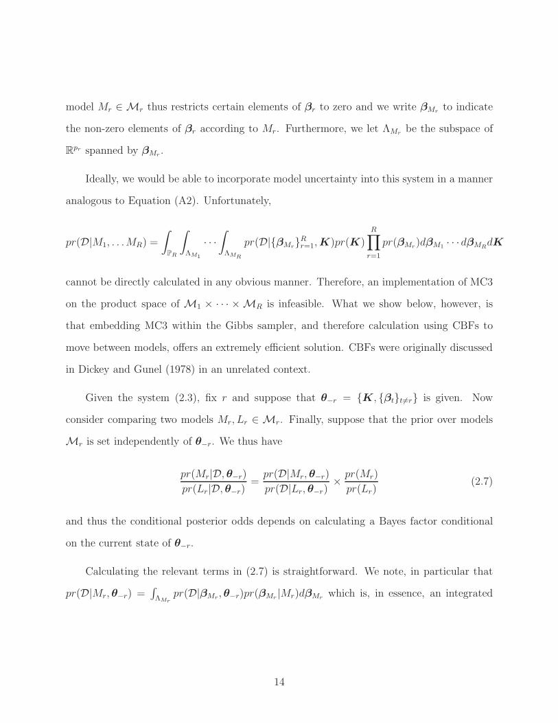
model Mr ∈ Mr thus restricts certain elements of βr to zero and we write βMrto indicate
the non-zero elements of βr according to Mr. Furthermore, we let ΛMrbe the subspace of
Rpr spanned by βMr
.
Ideally, we would be able to incorporate model uncertainty into this system in a manner
analogous to Equation (A2). Unfortunately,
pr(D|M1, . . .MR) =
∫
PR
∫
ΛM1
· · ·
∫
ΛMR
pr(D|βMrRr=1,K)pr(K)
R∏
r=1
pr(βMr)dβM1 · · · dβMR
dK
cannot be directly calculated in any obvious manner. Therefore, an implementation of MC3
on the product space of M1 × · · · × MR is infeasible. What we show below, however, is
that embedding MC3 within the Gibbs sampler, and therefore calculation using CBFs to
move between models, offers an extremely efficient solution. CBFs were originally discussed
in Dickey and Gunel (1978) in an unrelated context.
Given the system (2.3), fix r and suppose that θ−r = K, βtt6=r is given. Now
consider comparing two models Mr, Lr ∈ Mr. Finally, suppose that the prior over models
Mr is set independently of θ−r. We thus have
pr(Mr|D, θ−r)
pr(Lr|D, θ−r)=pr(D|Mr, θ−r)
pr(D|Lr, θ−r)×pr(Mr)
pr(Lr)(2.7)
and thus the conditional posterior odds depends on calculating a Bayes factor conditional
on the current state of θ−r.
Calculating the relevant terms in (2.7) is straightforward. We note, in particular that
pr(D|Mr, θ−r) =∫
ΛMrpr(D|βMr
, θ−r)pr(βMr|Mr)dβMr
which is, in essence, an integrated
14
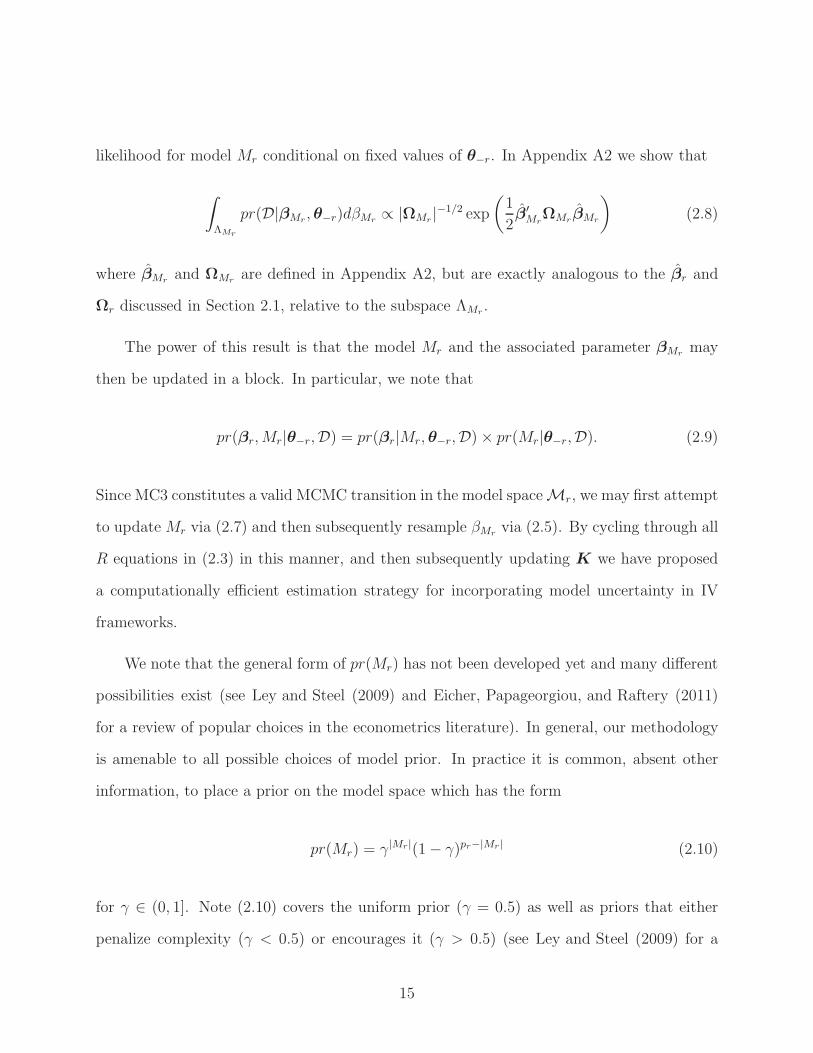
likelihood for model Mr conditional on fixed values of θ−r. In Appendix A2 we show that
∫
ΛMr
pr(D|βMr, θ−r)dβMr
∝ |ΩMr|−1/2 exp
(
1
2β′Mr
ΩMrβMr
)
(2.8)
where βMrand ΩMr
are defined in Appendix A2, but are exactly analogous to the βr and
Ωr discussed in Section 2.1, relative to the subspace ΛMr.
The power of this result is that the model Mr and the associated parameter βMrmay
then be updated in a block. In particular, we note that
Since MC3 constitutes a valid MCMC transition in the model spaceMr, we may first attempt
to updateMr via (2.7) and then subsequently resample βMrvia (2.5). By cycling through all
R equations in (2.3) in this manner, and then subsequently updating K we have proposed
a computationally efficient estimation strategy for incorporating model uncertainty in IV
frameworks.
We note that the general form of pr(Mr) has not been developed yet and many different
possibilities exist (see Ley and Steel (2009) and Eicher, Papageorgiou, and Raftery (2011)
for a review of popular choices in the econometrics literature). In general, our methodology
is amenable to all possible choices of model prior. In practice it is common, absent other
information, to place a prior on the model space which has the form
pr(Mr) = γ|Mr|(1− γ)pr−|Mr| (2.10)
for γ ∈ (0, 1]. Note (2.10) covers the uniform prior (γ = 0.5) as well as priors that either
penalize complexity (γ < 0.5) or encourages it (γ > 0.5) (see Ley and Steel (2009) for a
15
discussion of these features).
The key factor that a majority of priors considered in the literature share is their
treatment of each covariate as an independent unit, meaning that each affects the prior
probability independently. Without additional knowledge about the covariate set, this
assumption is a reasonable one, and we note that the IVBMA methodology discussed here
can incorporate all potential model priors of this form. However, as we discuss below, in the
context of many economic studies, the independent manner in which each variable enters the
model prior can have substantial negative consequences when variable inclusion probabilities
are used to assess the degree to which various theories are pertinent.
2.3 Priors in Theory Space
The critical issue of priors of the form (2.10) is their separability with regard to individual
covariates. As noted above, the prior (2.10) places an independent prior probability γ of
inclusion on each variable under consideration. However, in economic applications of model
uncertainty, variables are often meant to proxy theories. As they are proxies, they are
naturally imperfect and thus it is common to collect a number of different potential proxies.
Using posterior inclusion probabilies of these proxies to judge the relative strength of two
competing theories is then contaminated by the fact that differing numbers of proxies may
have been collected for each theory. Furthermore, the strong degree to which these proxies
are likely correlated with one another must be accounted for.
Model space priors which do not account for these multiplicity issues are liable to
overestimate the probability of those theories which are associated with the largest number
of variables. This occurs because the collection of models, including at least one constituent,
is greater than the set of models with few variables (see Durlauf, Kourtellos, and Tan (2011)
16
for a discussion). Therefore, economic studies utilizing model uncertainty to assess theory
relevance need to have model a prior which incorporate this structure.
In equation r of (2.3) suppose that there are Tr different theories. Let t ∈ 1, . . . , Tr = 9
denote one such theory with ptr potential variables included. Mtr is the model space defined
by theory t where Mtr ∈ Mtr when Mtr ⊂ 1, . . . , ptr with the restriction that Mtr 6= ∅.
Finally, let Xr,Mtrbe those columns of Xr associated with the model Mtr.
Setting priors in theory space is then performed hierarchically. Let γtr ∈ 0, 1 be
a binary indicator denoting whether theory t is relevant for equation r. We first set a
probability pr(γtr = 1) dictating our prior belief that theory t is relevant, which in practice
is typically chosen to be 0.5.
Subsequent to setting the prior overall probability that theory t holds, we then
set individual model-level probabilities inside each theory. The simplest prior that
corrects for multiplicity issues simply divides each theory by its size. But in practice,
multiple measurements that represent the same theory are likely to be highly correlated
and various priors have been proposed which account for this feature. The dilution
prior of Durlauf, Kourtellos, and Tan (2011) is a notable example but complicates the
straightforward implementation of the IVBMA algorithm discussed in Section 2.2. Both
priors are discussed in Appendix A3.
To alleviate this complication of the dilution prior, we instead use the auxiliary variable
γrt directly in each step of the sampler. Rewriting (2.3) we have
Yir =Tr∑
t=1
γrt(X′
r,Mrtθrt) + ǫir (2.11)
where γrt ∈ 0, 1, θrt ∈ ΘMrt, Mrt ∈ Mrt, ǫi ∼ N (0,K−1) and θrt ∈ ΘMrt
⊂ Rprt has zeros
according to the model Mrt. Let Mr = M1r, . . . ,MTrr be the collection of theory level
17
models for theory r write θr ∈ ΘMr⊂ R
pr to be the concatenation of parameter vectors
where each subset associated with a given theory t has the appropriate zeros according to
Mtr. Posterior inference can then proceed by sampling, in turn, the pair
pr(γrt,Mrt|·) = pr(γrt|Mrt, ·)pr(Mrt|·) (2.12)
for t = 1, . . . , Tr, and r = 1, . . . , R instead of the original sampling of Mr in Section 2.2.
Since any potential Mrt has the same denominator in Equation (A3), this term drops out of
pairwise comparisons.
In practice, resampling Mrt is performed by first forming
Ytr = Yr −∑
s 6=t
U(r)′
Msrθrs +
∑
q 6=r
Kqr
Krr
(Yq −U (q)′θq).
A neighboring M ′rt is then proposed, following the logic of (2.12), βMrt
and ΩMrtare
caculated using Ytr and Xr, which is combined with the prior probability pr(Mrt) to move
between the two competing models.
After resampling theMrt term, γrt is updated via pr(γrt = 1|Mrt, ·) =u1pr(γrt=1)
u1pr(γrt=1)+pr(γrt=0)
where u1 is calculated as in (2.8). If γrt is sampled to be 1, a parameter vector θrt ∈ ΘMrt
is resampled according to βMrtand ΩMrt
.
This sampling strategy, which relies heavily on the auxiliary variables γrt, allows for
complicated priors to be elicited inside a theory, without concern for the missing prior
denominator that would be necessary to directly compare a model Mrt ∈ Mrt to the null
model ∅ associated with the theory being invalid. Instead, by consistently updating which
model Mrt ∈ Mrt is to be compared to ∅ through the use of γrt we are able to move both
inside theory space and to turn off theories using roughly the same CBF machinery as above.
18
2.4 Assessing Instrument Validity
A critical assumption for the estimates of β1 to have appropriate inferential properties is that
the instrumental variables Z must be valid. In other words, E[Z ′iǫi1|ǫi2, . . . , ǫiR] = 0. Many
tools exist for evaluating the validity of this assumption in frequentist settings, the most
popular of which in the applied community is the test of Sargan (1958). To our knowledge,
consideration of similar assessments in a Bayesian setting have not been explored, beyond
the approximate test proposed in Lenkoski, Eicher, and Raftery (2014). In Appendix A4 we
propose a Bayesian assessment of instrument validity, borrowing many of the ideas above
and merging these with the spirit of the Sargan test.
Suppose that all residuals and K were known. Let ς be such that ςi = ǫi1+∑R
r=2K1r
K11ǫir.
The essential notion of the Sargan test is to consider the model ςi = Z ′iξ+ηi, ηi ∼ N (0, τ−1)
and test whether ξ 6= 0. The mechanics of the Sargan test ultimately rely on assymptotic
theory and Lenkoski, Eicher, and Raftery (2014) discusses its poor performance in low
sample size environments.
Our approach is to model this in a Bayesian context. In particular, we consider two
models: J0, which states that ξ = 0, and J1, which puts ξ ∈ Rq. We then aim to determine
whether pr(J0|D) is large, indicating instrument validity. Note that this can be represented
as the following marginalization
pr(J0|D) =
∫
pr(J0|ς,D)pr(ς|D)dς (2.13)
This approach offers similar performance to the test of Sargan (1958) and has the
desirable features that it is a fully Bayesian approach (as opposed to the approximate
test of Lenkoski, Eicher, and Raftery (2014)), which can be directly embedded in the Gibbs
19
sampling procedures outlined above. Much work can still be done on this diagnostic.
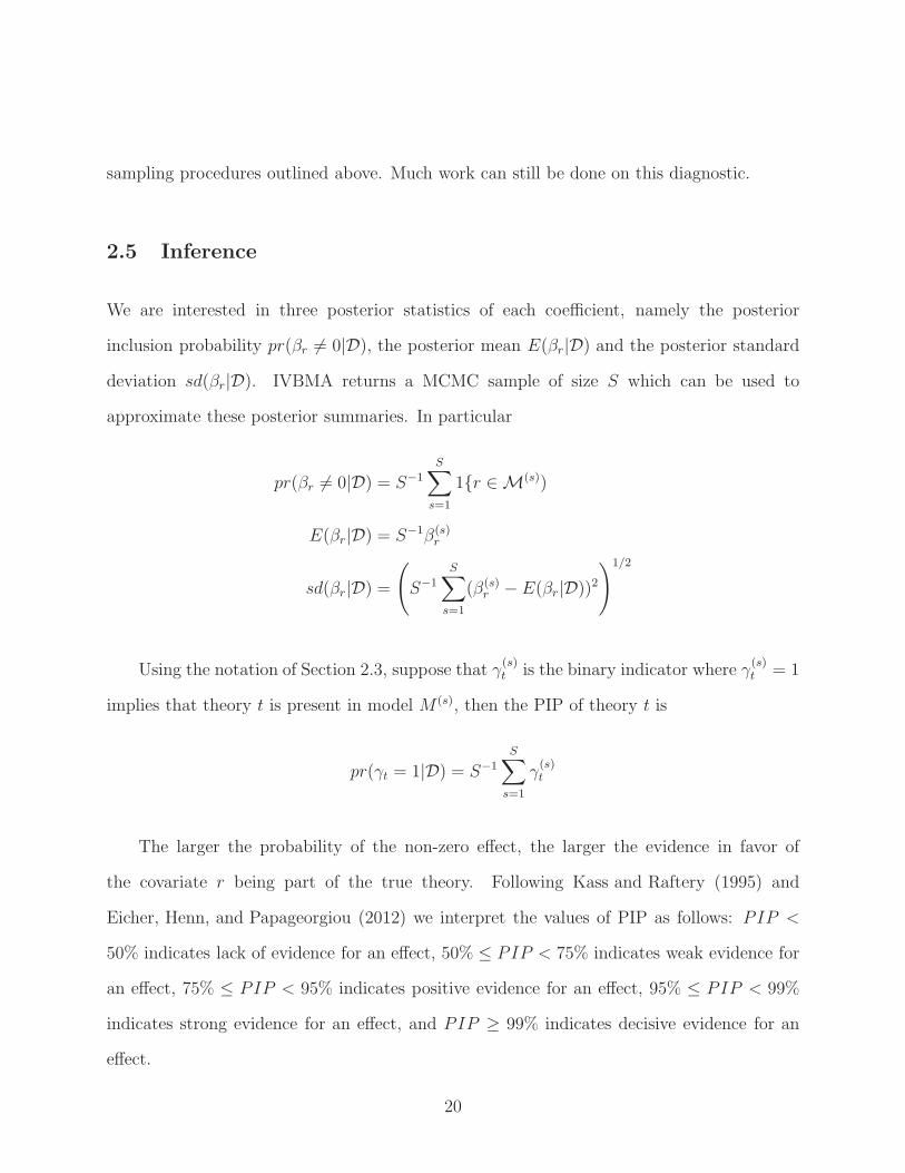
2.5 Inference
We are interested in three posterior statistics of each coefficient, namely the posterior
inclusion probability pr(βr 6= 0|D), the posterior mean E(βr|D) and the posterior standard
deviation sd(βr|D). IVBMA returns a MCMC sample of size S which can be used to
approximate these posterior summaries. In particular
pr(βr 6= 0|D) = S−1S∑
s=1
1r ∈ M(s))
E(βr|D) = S−1β(s)r
sd(βr|D) =
(
S−1
S∑
s=1
(β(s)r − E(βr|D))2
)1/2
Using the notation of Section 2.3, suppose that γ(s)t is the binary indicator where γ
(s)t = 1
implies that theory t is present in model M (s), then the PIP of theory t is
pr(γt = 1|D) = S−1
S∑
s=1
γ(s)t
The larger the probability of the non-zero effect, the larger the evidence in favor of
the covariate r being part of the true theory. Following Kass and Raftery (1995) and
Eicher, Henn, and Papageorgiou (2012) we interpret the values of PIP as follows: PIP <
50% indicates lack of evidence for an effect, 50% ≤ PIP < 75% indicates weak evidence for
an effect, 75% ≤ PIP < 95% indicates positive evidence for an effect, 95% ≤ PIP < 99%
indicates strong evidence for an effect, and PIP ≥ 99% indicates decisive evidence for an
effect.
20
3 Measurement Issues
We employ a 5-year period unbalanced panel of 91 countries from 1971 to 2010.10 The
data are averaged over 5 years to avoid business cycle effects. To form five year panels
from annual data, we took the arithmetic averages of the available annual values for each
variable. The countries and observations vary by the category of expenditure used. For the
total government expenditures we have information on 91 countries, while for the various
components we have information on 80 countries. Details about the countries can be found
in Table S2 of Supplementary Online Appendix.
3.1 Government Expenditure
We measure government size in complementary ways, one by general expenditure and the
other by central government expenditure. Government expenditure is further classified by
economic or functional classification. For the economic classification of expenditure, we
use expenses for “Compensation of employees” and “Use of goods”. For the functional
classification of expenses we use expenses for “General public services”, “Defence”, “Public
order and safety”, “Economic affairs”, “Health”, “Education” and “Social protection”.11 The
source for the share of government expenditure to GDP is the IMF’s Government Financial
Statistics database (GFS). Information on total government expenditure and its components
can be found in Table S3 of Supplementary Online Appendix, and the summary statistics in
Table S5 of Supplementary Online Appendix.
10We extend Shelton (2007) in two dimensions, time and determinants. Shelton (2007) uses a 5-yearperiod unbalanced panel of a similar set of countries from 1971 to 2000. We use the same set of governmentexpenditure components, but we use a much broader set of determinants.
11Following Persson and Tabellini (1999) and Shelton (2007), expenditure of public good is the sum ofpublic order and safety, health and education expenditures.
21
3.2 Determinants
The determinants of government expenditure are organized into nine different theories:
Centralization, Conflict, Country Size, Demography, Globalization, Income Inequality,
Macroeconomic Policy, Political Institution and Wagner’s Law, as discussed in the
introduction. Measuring these theories results in 19 proxies from several databases.12
Additionally, in every model we include a constant, time, and country fixed effects.
For Centralization we use the ratio of central to general total government expenditure
from GFS. We proxy Conflict using the warfare score. We use the natural logarithm of
the population and the natural logarithm of the country’s land area in square kilometers to
proxy Country Size. For Demography we use the share of people younger than 15 years old
and older than 64 years old to the working age population, the share of urban population
to total population and population growth. We proxy Globalization with trade openness
and Income Inequality with the Gini coefficient for gross inequality. Macroeconomic Policy
is proxied by the share of central government debt to GDP, the natural logarithm of FDI
liabilities stock, and inflation. For Political Institution we use the combined polity score,
the political competition index, the political rights index, the presidential system dummy,
and the plurality dummy. Finally, for Wagner’s Law we use the natural logarithm GDP
per capita. Information on all the determinants can be found in Table S4 of Supplementary
Online Appendix, the summary statistics in Table S6 of Supplementary Online Appendix,
and correlations in Table S7 of Supplementary Online Appendix.
12The Database of Political Institutions (DPI), the Freedom House (FH) database, theHistorical Public Debt Database (HPDD), the IMF’s Government Financial Statistics database(GFS),Lane and Milesi-Ferretti (2007), the Major Episodes of Political Violence database (MEPV), PennWorld Table 8 (PWT), Political Regime Characteristics and Transitions, the 1800-2013 database of thePolity IV Project (PRCT), the Polity IV Project (PIV), Solt (2009) and the World Development Indicatorsdatabase (WDI).
22
4 Results
In this section we present the results for our baseline results as well as a number of additional
investigations that aim at providing a sensitive and in-depth analysis. First, we present the
posterior inclusion probability (PIP) of the theories and the determinants, the posterior
mean, and posterior standard deviation of the determinants, for both general and central
government expenditures.
Second, in order to identify the contribution of each theory and determinant to the
variation of total expenditure (and in its components), we construct a variance decomposition
analysis. Third, we present results for the channels of transmission, in order to cast more light
on the importance and the magnitude of the various theories. This analysis can also serve
as a robustness for our theory priors. Last but not least, we provide a deeper investigation
on the effect of globalization, and income inequality.
4.1 Total Government Expenditure and Components
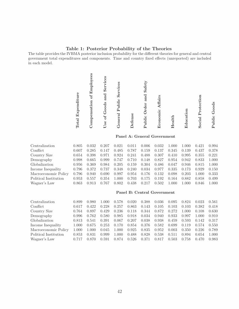
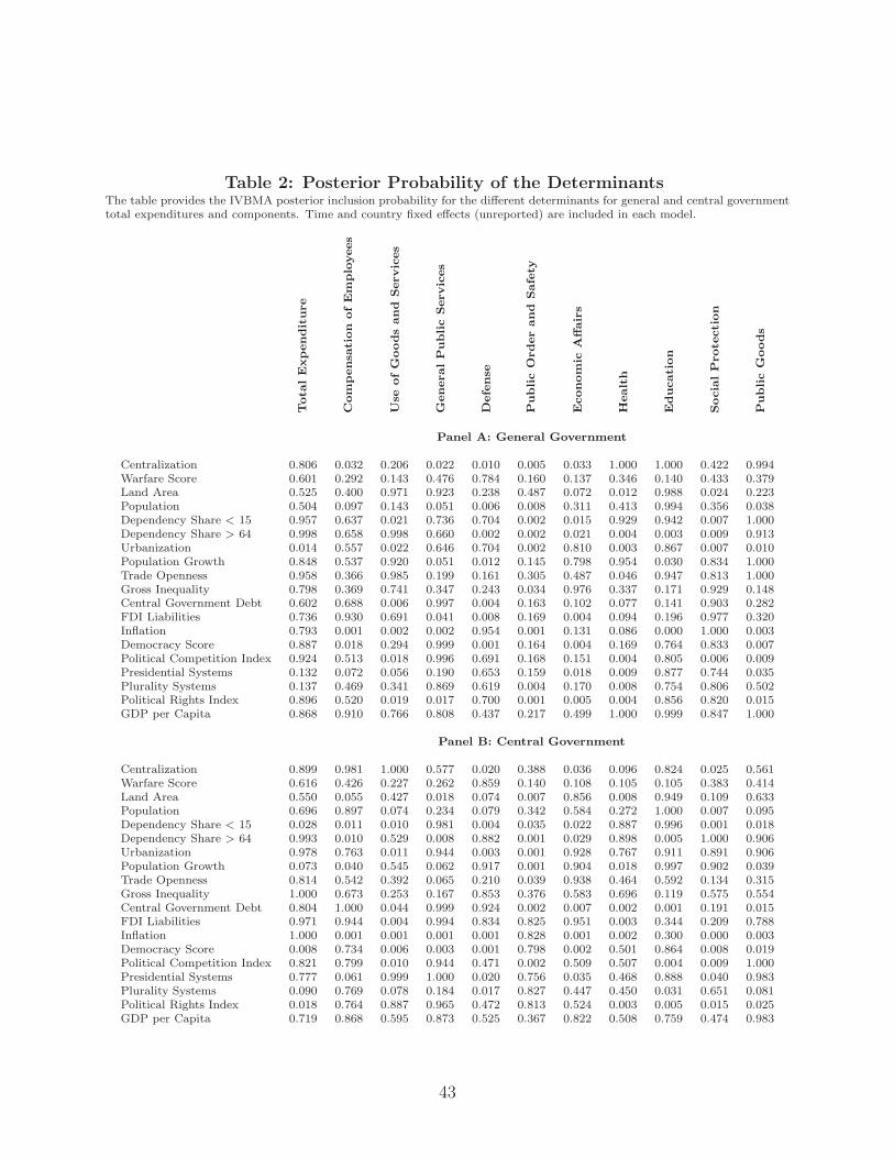
The PIPs of the theories and determinants are presented in Tables 1 and 2, respectively.
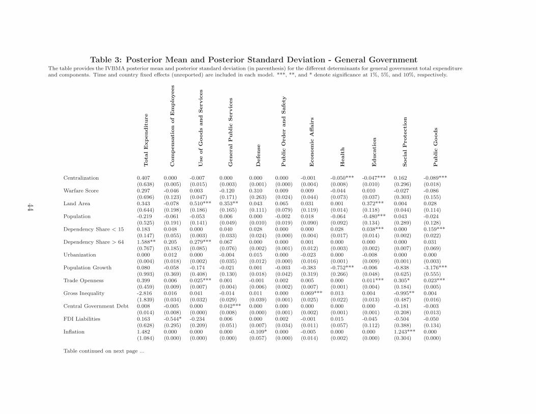
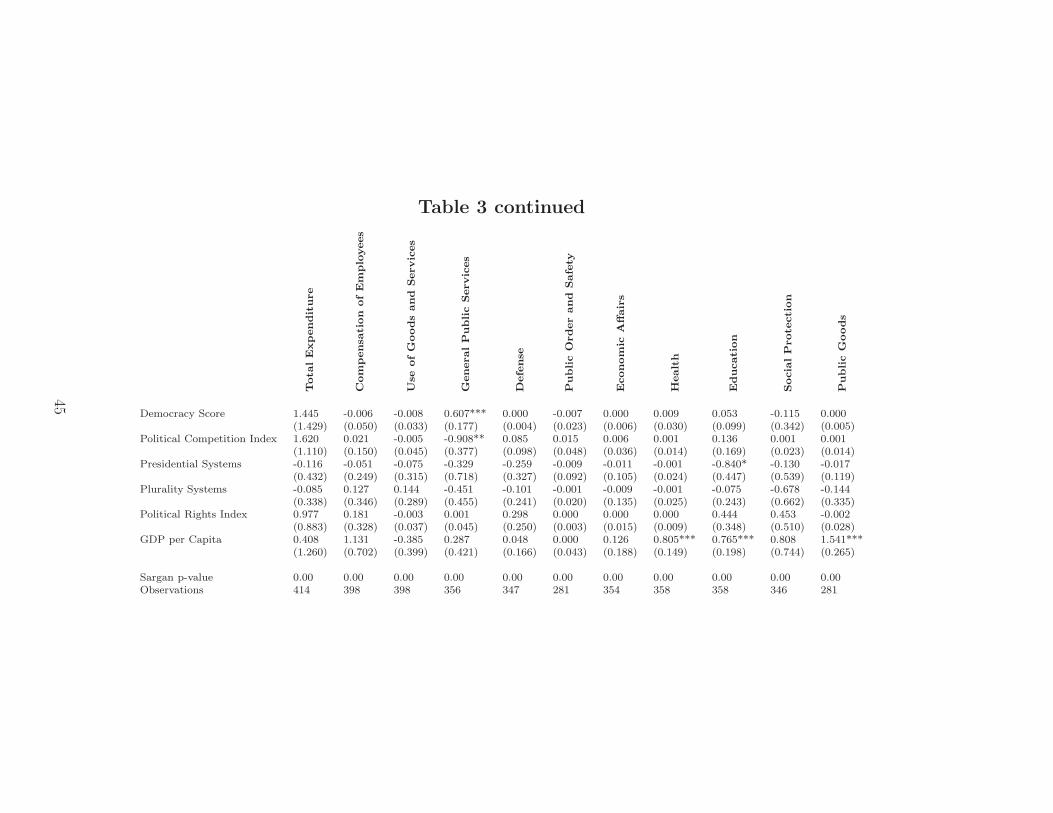
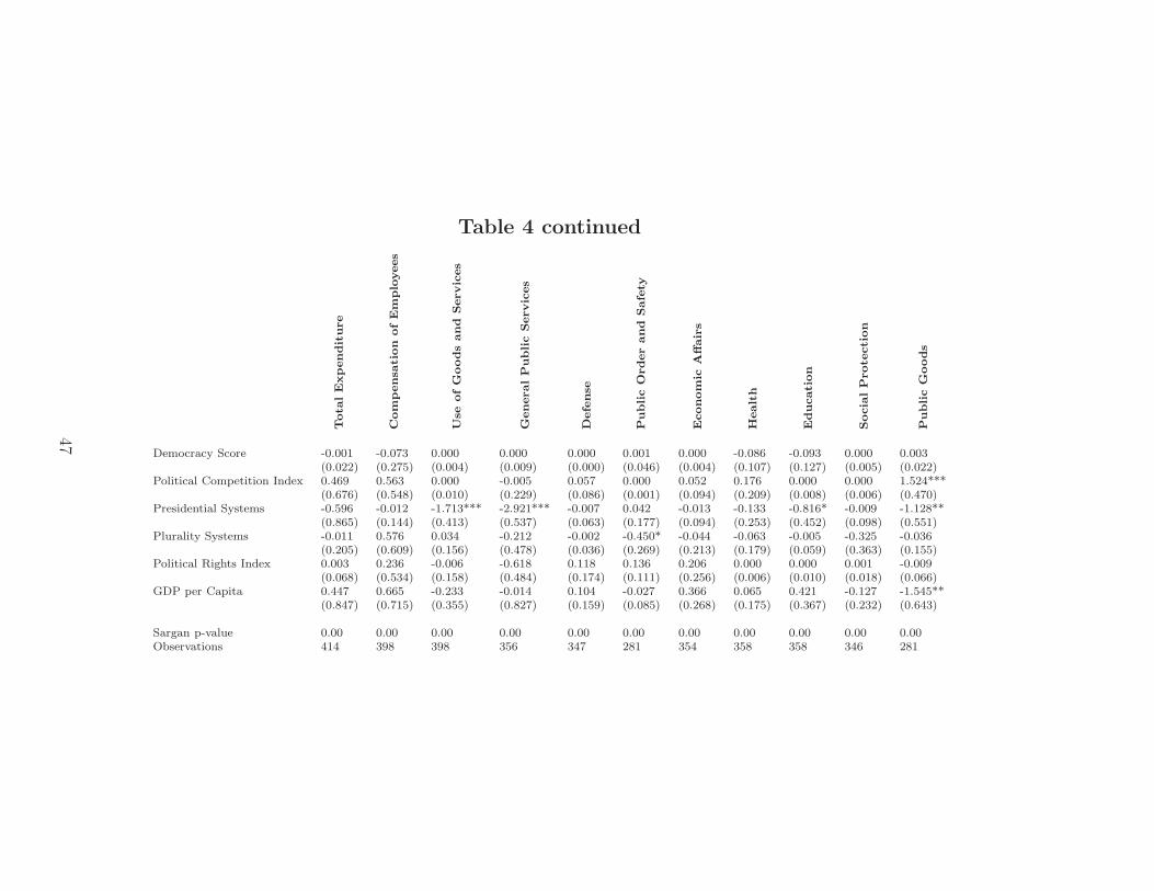
Tables 3 and 4 present the posterior means and the posterior standard deviations of the
determinants, for the general and central government expenditures, respectively. The first
column of the tables shows the theories; the second column presents results for total
expenditure; and the remaining columns present results for the components.
4.1.1 General Government
Results suggest that the theory of demography has a decisive impact on general government
total expenditure and strong evidence for the theories of globalization and political
23
institution. We also find positive evidence for Wagner’s law, centralization, income inequality
and macroeconomic policy theories and some weak evidence for the country size and conflict
theories.
In particular, the posterior inclusion probability of the demography theory is 0.998. As
seen from Table 2, column 2, and Table 3 this is due to the decisive effect, with a positive
posterior mean, of the ratio of the population older than 64 (PIP = 0.998), the ratio
of the population younger than 15 years old (PIP = 0.957), and the population growth
(PIP = 0.848). The effect of demography on total government expenditure pertains to its
effects on the components. More precisely, demography theory has a decisive role for public
goods expenditure (health and education) through the share of the population younger than
15 and older than 64. This is consistent with the explanation of Cassette and Paty (2010),
that the share of the population over 65 constitutes an interest group with high political
power, voting for social benefits programs, such as health. Population growth has a negative
effect on the use of goods and services, social protection and public goods expenditure. Given
the fixed cost (establishing a set of institutions) and the economies of scale linked to partial
or complete non-rivalry in the supply of public goods, the population growth decreases the
expenditure as a % of GDP.
Results suggest that globalization plays a strong role for the total expenditure with
PIP equal to 0.956. This evidence pertains to decisive evidence, with positive posterior
mean, of globalization, with positive posterior mean, on the public goods expenditure
(through education), strong evidence, with positive posterior mean, on the use of goods and
services expenditure and positive evidence on the social protection expenditure. Our results
are generally consistent to those of Rodrik (1998) who finds that globalization increases
inequality and economic insecurity, which from the demand side of the political market
create incentives for government to compensate the losers, mainly through income transfer
24
programs and economic policy activism. Our results are generally consistent with these
findings, since we find a positive effect on both the direct (social protection) and indirect
(public goods) form of transfer. A more detailed analysis will be delayed until Section 4.4.1,
using a smaller sample.
We also find strong evidence for the political institution theory, with PIP = 0.953.
Specifically, we find positive evidence for the political competition index, the political right
index, and the democracy index. The positive effect of the democracy index on total
expenditure (through the general public services and education expenditures) is consistent
with Alesina and Wacziarg (1998). They find that democracies have higher government
size due to the fixed cost in building democratic institutions, and the existence of social
and redistribution policies. In contrast, we find a negative effect on the social protection
expenditure, which is a direct form of redistribution. This can be explained by the presence of
many pressure groups in democracies, which may lead to greater heterogeneity of preferences
and thus, lower levels of redistribution. Instead, our results seem to support the political
competition theory by Eterovic and Eterovic (2012) that the increase in political competition
is likely to decrease government expenditure, which is found in our results for the general
public services expenditure.13 Shelton (2007) argues that as political rights become more
open, more social and redistribution policies that take place. Again our results are consistent
with this.
Furthermore, we find positive evidence for Wagner’s law, centralization, income
inequality and macroeconomic policy theories, and weak evidence for the country size and
conflict theories. Our results are consistent with Wagner’s Law theory, as suggested by the
13As Eterovic and Eterovic (2012) state there are at least four reasons why enhanced political competitionis likely to decrease government expenditure: (1) the theory of fiscal illusion, (2) enhanced politicalcompetition allows more pressure groups to be catered to in the political calculus, (3) political competitionenhances political accountability, and (4) in societies with severe restrictions on political competition(dictatorship) political leaders need to spend substantial public funds on securing and maintaining power.
25
positive posterior mean for total expenditure and the public goods and the social protection
expenditures.14 The positive posterior mean of the centralization theory is consistent with
the Brennan and Buchanan (1980) hypothesis.15
Finally, the negative posterior mean of the Gini coefficient is in contrast to the majority
voting hypothesis (Meltzer and Richard (1981)). The literature suggests that inequality
may negatively affect redistribution, if we take into account capital market imperfections
(e.g., Roemer (1998), Benabou (1996) and Benabou (2000)), in the presence of high
intergenerational mobility (Benabou and Ok (2001)) or if redistribution is accomplished by
a public provision of goods and services rather than by transfers (Grossmann (2003)). In
particular, we find strong evidence for the effect of Gini on social protection expenditure.
This result suggest that a deeper investigation of the mechanism that drives this is needed.
This is done in Section 4.4.2. Additionally, we find strong evidence for the effect of inequality
on economic affairs expenditure. Note that economic affairs can be viewed as a form of public
goods that contain among other, expenses on labor affairs, fuel and energy, manufacturing,
transport and communication.
4.1.2 Central Government
As in the case of the general government, we find that the majority of the proposed theories
provide us with at least positive evidence on the central government expenditure. Compared
with the general government we find decisive evidence for the theories of macroeconomic
14Wagner’s law suggests that as states grow wealthier they simultaneously grow more complex, increasingthe need for public regulatory and protective action to ensure the smooth operation of a modern, specializedeconomy. Additionally, it postulates that certain public goods, such as education and health, are luxurygoods, which means that the demand for those goods increases more than proportionally as income rises.Finally, Shelton (2007) indicate that richer countries have a bigger fraction of people over 64 years old, whodemand more social protection.
15Brennan and Buchanan (1980) suggest that an increase in fiscal centralization will lead to more totalgovernment spending.
26
policy and income inequality on central government total expenditure, in addition to
demography. Central government includes expenditures of political authority that extends
over the entire territory of the country.
Macroeconomic policy theory decisively affects total government with PIP equal to
1, through inflation (PIP = 1) and FDI liabilities (PIP = 0.971). Consistent with
Zakaria and Shakoor (2011), we find a negative effect of inflation on total expenditure. This
can be explained by the shrinking size of the formal sector or the reductions of the real value
of government revenues, which limit the government’s ability to spend. Importantly, our
results do not support the hypothesis of the reduction of government size in order to increase
competitiveness to attract FDI, given that we find a positive effect on central government
total expenditure. This comes through an increase in general public services and public
order and safety, which includes expenditure on executive and legislative organs, financial,
fiscal and external affairs and expenditure on police protection services and law courts, which
are the main mechanism in attracting and preserving foreign direct investments. The weak
evidence of FDI on general government expenditure suggest that FDI related policies are
adopted in the central government and lower levels (state or local).
We also find decisive evidence, with positive posterior mean, for the income inequality
theory, with PIP = 1, indicating that as inequality increases, so does the government size.
Interestingly, we only find weak evidence of the effect of income inequality on the components.
As in the case of general government, the Meltzer and Richard (1981) hypothesis is not
supported, since we do not find any effect on neither social protection nor public goods
expenditure. Given that total expenditure is the summation of the various components, we
can conclude that the summation of the weak evidence of the effect of income inequality on
the components provide the decisive evidence of the effect on total expenditure. In particular
we get a small positive effect on the components (use of goods and services, economic
27
affairs, public order and safety, health, and education expenditures), which summing those
we end up with the positive effect on total expenditure. Given that general government
is the summation of central and local government then the effect of inequality on general
government economic affairs and social protection expenditures, comes from the local level,
since in the central level we do not find any effect.
For the rest of the theories, results are similar to those relating to the general government.
Specifically, we find decisive evidence for the demography theory, positive evidence for
the centralization, political institution, globalization, and country size theories, and weak
evidence for Wagner’s law and conflict theories. Finally, we find notable differences between
general and central government on the effect of urbanization and the presidential dummy.
For the former, we find a positive posterior mean on public goods and social protection
expenditure, which support the Ferris, Park, and Winer (2008) hypothesis.16 Additionally,
the negative effect on both general public services and economic affairs expenditure, can
be explained by economies of scales, since government expenditure on administration,
regulation, and operation are gathered in urban regions. The negative posterior mean of
the presidential dummy on the use of goods and services, general public services and public
goods expenditure (similar results with the general government) is consistent with Baraldi
(2008).17
4.1.3 Instrument Validity
Reliability of inference requires instrument validity. Hence, in this section we employ the
diagnostic test proposed in Section 2.4 to evaluate the validity of the instrument.
16They suggest that as urbanization increases, a greater demand for government services is expected ifeducation and health are mainly public responsibilities.
17He suggest that in presidential regimes government tends to be more efficient due to the competitionbetween the policy makers.
28
In the bottom part of Tables 3 and 4 we present the p-value of our test statistic, under
the null of no validity of the instruments, for general and central government, respectively.
For both the general and the central government total expenditures and its components we
reject the null hypothesis that the instruments are not valid. This result provides strong
evidence that the instruments we use are valid across all cases.
4.1.4 Summary of the Main Findings
The main finding is that the effect of the proposed theories on government expenditure is
multidimensional. We find substantial evidence that total expenditure and its components
are explained by different theories. However, the effect of the various theories differs in
terms of its significance, size and the specific measure of government size. On the one
hand, for general government total expenditure we find decisive evidence for the demography
theory and strong evidence for the theories of globalization and political institution. On the
other hand, for the central government total expenditure we find decisive evidence for the
demography, macroeconomic policy, and income inequality theories.
In the next section, we present the results for the variance decomposition analysis.
4.2 Variance Decomposition
In this section, we develop a variance decomposition analysis, in order to determine
the contribution of each theory in explaining the variation of total expenditure and its
components. Firstly, we compute the posterior mean of each theory t: Tt = Xt,1βt,1 +
Xt,2βt,2+ ...+Xt,pβt,p, where βt,j is the set of estimates for the coefficients of the determinants
for theory t. Following Klenow and Rodriguez-Clare (1997), we decompose the variance of
29
each theory:
1 =Tr∑
i=t
Cov(govj, Tt)
V ar(govj)+Cov(govj, et)
V ar(govj), t = ., . . . , Tr
The results from the Balanced Variance Share (BVS) are presented in Table 5. Additionally,
we provide robustness analysis in Table S8 of Supplementary Online Appendix, using
Correlated Variance Share (CVS) as an alternative decomposition method, finding similar
results.18
The variation of general government total expenditure is mainly explained by the
demography theory (40.3%), the political institution theory (38.3%), the centralization
theory (22.6%), and the income inequality theory (6.7%). Furthermore, the globalization
(3.4%) and Wagner’s law theory (3%), seem to explain only a small part of the total
expenditure variation. For the central government total expenditure, only the demography
theory explains a large fraction of the variation (32%). One notable difference is that while
the macroeconomic policy and income inequality theories exhibited a decisive role in terms
of PIP, their impact in terms of their ability to explain the variation of expenditure is small,
suggesting that the effect is significant but small in magnitude. With the exception of the
conflict and the country size theories, all others explain a fraction between 3% and 9% of
the variation of central government total expenditure. Importantly, our results show that
country and time heterogeneity do not explain the variation of total expenditure, neither on
the general nor the central level.
In sum, our results are in agreement with the results from the posterior inclusion
probability. The determinants that have a high PIP explain more than 5% of the various
expenditures components variation.
18BVS is calculated as the share of the covariance between the posterior mean of theory t and of expenditure
category j, to the variance of expenditure category j: BV S =cov(Trt,govj)var(govj)
. CVS is calculated as the
share of the posterior mean of theory t to the variance of expenditure category j: CV S = var(Trt)var(govj)
. See
Gibbons, Overman, and Pelkonen (2014).
30
4.3 Channels of Transmission Analysis
In this section we consider two complementary investigations to identify and explain the
mechanisms that underlie the estimated relationships between the various theories and
government expenditure. First, we exclude a theory from the model space one at a time
in a similar fashion as the mediation analysis, but rather than focusing on individual
variables, here, the unit of analysis are the theories and their proxies. In such an analysis,
the hypothesis is that an underlying theory transmits its effect to government expenditure
directly as well as indirectly via a mediator theory. For example, political institutions can
affect government expenditure directly or indirectly via their effect on globalization. By
excluding the globalization theory from the model space we can assess its mediation role vis-
a-vis the other theories of the government expenditure using a posterior odds ratio analysis.
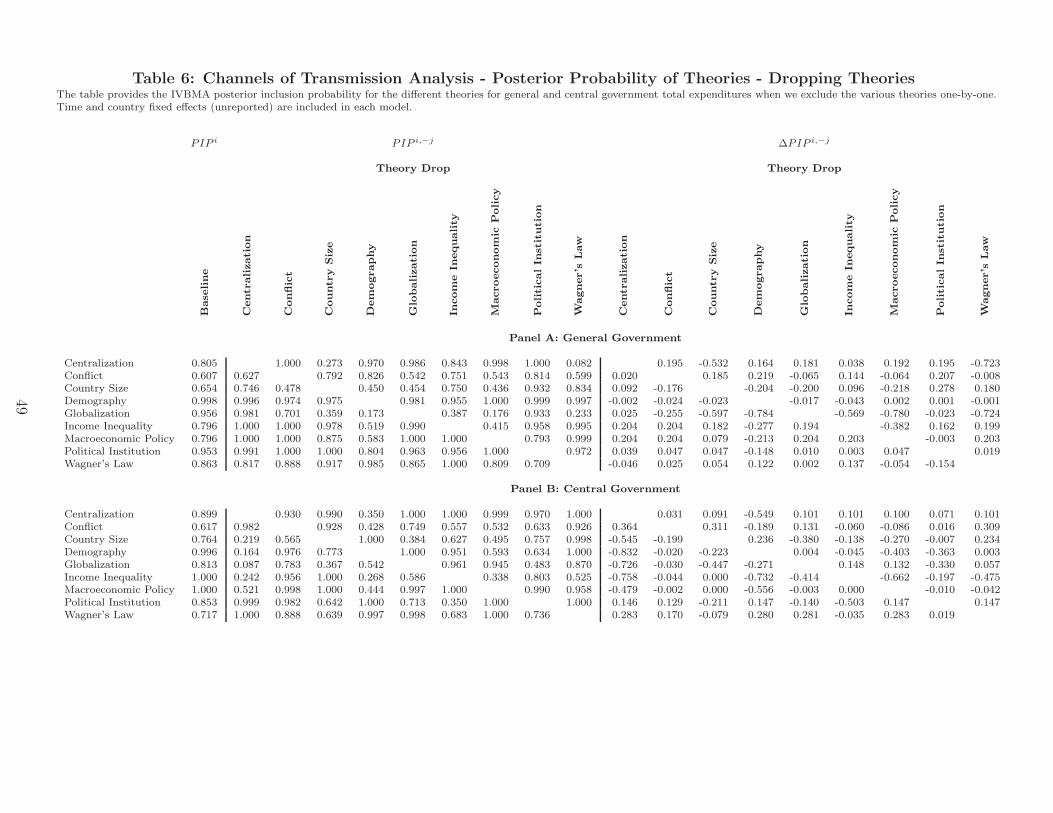
For any two given theories i and j, i 6= j we estimate
PIP i
PIP i,−j+
∆PIP i,−j
PIP i,−j= 1, (4.14)
where PIP i is the posterior inclusion probability of theory i in the baseline model, which
gives us the direct effect of theory i on government expenditure, PIP i,−j is the posterior
inclusion probability of theory i after we exclude the theory j and ∆PIP i,−j = PIP i,−j −
PIP i is the difference of the two, which gives us the mediation effect.
The posterior inclusion probabilities of the theories and the decomposition into direct
and mediation effects are presented in Table 6. Additionally, in Tables S9 and S10 of
Supplementary Online Appendix we present the direct and the mediation effect of the
posterior inclusion probabilities and the posterior mean of the determinants, respectively.
As described in the basic model analysis, for the general government total expenditure, only
the demography theory has a PIP higher than 99%. This effect is mainly driven by the share
31
of the population younger than 15 and older than 64. When we exclude any other theory,
we always find the same decisive evidence for the effect, indicating a very small mediation
effect. Examining the individual variable, we find that the mediation effect is much higher
both in terms of PIP and posterior mean. For example, excluding the macroeconomic policy
theory, we find that the PIP for the share of the population younger than 15 drops from
0.957 to 0.027 and the share of the population older than 64 drops from 0.998 to 0.051.
In addition, the posterior mean becomes almost zero, from 0.183 and 1.588 for share of
population younger than 15 and older than 64, respectively.
For the theories with a PIP higher than 95% (globalization, and political institution) in
the baseline model, we find that with the exception of centralization and political institution
theories, excluding any theory causes a decrease of the PIP in globalization to less than
75% and a sharp decrease of its posterior mean (in some cases the effect of trade openness
becomes negative). In contrast, the exclusion of any theory causes a small positive mediation
effect on the political institution theory, meaning that the PIP, increases. This is true for
all cases with the exception of the case which we exclude demography theory and find that
PIP decreases from 0.953 to 0.804. The mediation effect on the PIP of the determinants is
relatively higher than the mediation effect on the PIP of the theories.
The results for the central government total expenditures and its components are
generally similar. In the baseline model we find decisive evidence for the effect of demography,
income inequality, and macroeconomic policy theories. The mediation effect of the PIP of
the macroeconomic policy theory is big only for the cases in which we exclude either the
centralization or the demography theory. This is mainly due to the sharp decrease of PIP
and posterior mean of FDI and inflation. For the demography and income inequality the
mediation effects in PIP are relatively large, in the sense that the initial PIP of the theories
change substantially with the exclusion of the majority of the theories.
32
In sum, this analysis shows that most of the theories affect government expenditure
directly as well as indirectly. In particular, while globalization theory has a big effect on
general government expenditure, in terms of PIP and posterior mean, it also has a big indirect
effect through the majority of the other theories. This is also true for the overall effect of the
demography and income inequality theories on central government expenditure. Finally, we
find that the indirect effect of macroeconomic policy theory comes from the centralization
and the demography theories.
Second, we undertake an alternative investigation that conditions on a treatment theory
to be always present in all models and then ask the question of how model uncertainty with
respect to the remaining theories, which are viewed as controls, influence the effect of the
treatment theory. Results for the PIP of the theories are presented in Table 7. In Tables S11
and S12 of Supplementary Online Appendix we present the direct and the mediation effect
of the posterior inclusion probabilities and the posterior mean of the determinants. For both
general and central government total expenditure we find that the impact of conditioning on
a theory to always be included in the model space is quite substantial. For example, in the
case of the general government total expenditure, when we condition Wagner’s law theory to
be included in the model space we find that while the PIP of the demography theory drops
from 0.998 to 0.703 (∆PIP i,−j = −0.295), the PIP of the macroeconomic policy theory rises
from 0.796 to 0.995 (∆PIP i,−j = 0.199).
Overall, this analysis highlights the presence of model uncertainty and the vital role of
BMA in order to obtain valid inference. This analysis also illustrates that while the BMA
does not depend on individual models, it does depend on the model space. Thus, to ensure
correct specification of the model space we included in the analysis all the relevant theories
to the best of our knowledge.
33
4.4 Further Results
In this section we provide an in-depth analysis of globalization using a smaller sample and
a deeper look in the relationship between government size and inequality by allowing for
heterogeneity in the effect of income inequality.
4.4.1 Globalization
As argued by Rodrik (1998) the exposure to risk of the more open to trade economies can
be mitigated by increasing the “safe” government sector. Following Rodrik (1998) we use
the terms of trade variability as proxy of risk. The interaction term of trade openness and
terms of trade variability measure the external risk for an open economy.19 The inclusion of
these additional terms limit our sample substantially (85 countries and 219 observations),
which explains the reason we opted not to consider this in the baseline sample.
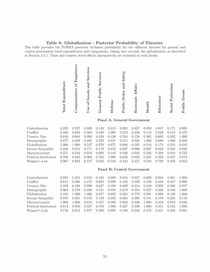
In Table 8 and Table S13 of Supplementary Online Appendix we present the PIP of the
theories and the variables, respectively. We find a decisive effect with PIP equal to 1 for
the globalization theory on the general government total expenditure. While the PIP of the
interaction term is equal to 1, indicating decisive evidence for the effect, the posterior mean is
negative. Additionally, the PIP of the interaction term on both social protection and public
goods expenditures indicates that neither matters (PIP is 0.003 and 0.038, respectively). In
the case of central government level, we find decisive evidence for the effect of globalization
on public goods expenditure. The PIP of the interaction term is 1, but the posterior mean
is negative. These results do not support the explanation of Rodrik (1998), who finds a
positive effect.
19Rodrik (1998) finds a positive and statistically significant coefficient for the interaction terms.
34
4.4.2 Income Inequality
Both the theoretical and the empirical evidence for the effect of income inequality theory on
government size is inconclusive. On the one hand, Meltzer and Richard (1981) hypothesis
suggests that income inequality can generate demand for more redistribution and a larger
government. On the other hand, there are theories suggesting that inequality may negatively
affect redistribution, in the presence of capital market imperfections (e.g., Roemer (1998),
Benabou (1996) and Benabou (2000)), in the presence of high intergenerational mobility
(Benabou and Ok (2001)) or if redistribution is accomplished by a public provision of goods
and services rather than by transfers (Grossmann (2003)). We find a negative strong
evidence for the effect of Gini on general government social protection expenditure and a
positive decisive evidence on central government total expenditure, but only weak evidence
of the effect of income inequality on the various components. As a next step we allow for
heterogeneity in income inequality, by replacing the Gini variable with interactions of the
Gini with income group dummy variables as reported by the World Bank.
In Table 9 and Table S14 of Supplementary Online Appendix we present the PIP of
the theories and the variables, respectively. We find a decisive effect (PIP = 1) for the
income inequality theory on general government total expenditure and a positive evidence
(PIP = 0.853) on central government total expenditure. The effect on general government
comes from social protection expenditure and on central government comes from public
goods expenditures. In both case we find a decisive evidence for the effect with PIP equal
to 1. The rest of the theories are consistent with the baseline model.
In particular for general government social protection expenditure we find a positive
effect of income inequality in lower income countries (PIP = 0.893), a negative effect in
lower middle income countries (PIP = 1) and an insignificant effect in upper middle income,
35
and in high income countries (PIP = 0.006 and PIP = 0.004 respectively). This results are
closer to the Prospect of Upward Mobility (POUM) hypothesis of Benabou and Ok (2001).
In low income countries, intergenerational income elasticity is higher than in lower middle
income countries.20 In the lower middle countries, individuals may choose not to support
high tax rates because of the prospect that they, or their children, may move up in the
income distribution ladder and therefore be hurt by such policies.
For the central government public goods expenditure we find a positive effect of
inequality only for high income countries, while for the rest of the countries we find a negative
effect. For example this is consistent with Benabou (2000) who examines the role of the
presence of capital market imperfections. In the presence of credit constrains, redistribution
will command less political support in an unequal society than in a more homogeneous one.
Additionally, Grossmann (2003) shows that if redistribution is accomplished by a public
provision of goods and services rather than by transfers.
4.5 Robustness
4.5.1 Parameter Heterogeneity
We generalize the analysis we undertaken in Section 4.4.2 for all theories. We investigate
parameter heterogeneity, with respect to the income group of each country, as reported by
World Bank. We replace each theory with four new theories, based on income group. We use
the interaction of the variable with the income group dummies (high income, upper middle
income, lower middle income, and low income), which they add up to the original variable.
20Some evidence are provided in Hertz, Jayasundera, Piraino, Selcuk, Smith, and Verashchagina (2007).For example, for low income countries they find a coefficient of 0.75 and 0.94 for Ethiopia has and Nepal,respectively. For lower middle countries they find a coefficient of 0.41 and 0.61 for Philippines has and SriLanka, respectively.
36
Then each variable is included in the relevant theory. The results for the PIP for the theories
and variables are presented in Table 10 and Table S15 of Supplementary Online Appendix,
respectively.
For general government we find decisive evidence for the demography theory. Splitting
the theory into the 4 income groups we find a strong evidence only for the high income
countries. This is consistent with the fact that in those countries both the percentage
of people older than 64 and the percentage of urban population is higher, than in lower
income countries. For globalization and political institution theories, that we find a strong
evidence, parameter heterogeneity plays an important role. The PIP of the globalization
theory is higher than 95% only for high income countries (this is reasonable given that
those countries are more open to international trade). The strong evidence of the political
institution theory is not found in any of the four income groups (we find a positive evidence
only for upper middle income countries). Our baseline results suggest a decisive evidence
for the macroeconomic policy, income inequality, and demography theories. As in the case
of general government total expenditures the PIP for those theories is much higher for the
high income countries.
From the whole set of results we can conclude that parameter heterogeneity affects the
formation of both general and central government total expenditures. More importantly,
the evidence of parameter heterogeneity does not invalidate our previous results but simple
provides a deeper understanding of the effect of the various theories.
4.5.2 Theory Prior
Our proposed method, discussed in Section 2.3, overcomes the multiplicity issues due to the
fact that several competing theories are simultaneously tested and each theory has a number
37
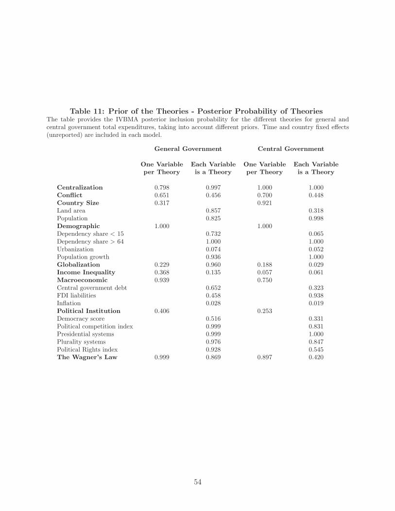
of variables which serve as potential proxies. Here we consider a robustness exercise that
sets flat weights on each theory. We consider two cases. First for each theory we include
only a single variable.21 Second we set that each determinant is a theory by its own. Results
are presented in Table 11.
In the case of including a single variable, in terms of theory PIP we find that for
general government globalization, income inequality and political institution theories lose
their significance while now we find a decisive effect for the Wagner’s law theory. For central
government we find that globalization, income inequality and macroeconomic theory lose
their significance while country size PIP increase to 1.
In the second case, when we treat each variable as a single theory. We find positive
evidence for both variables of the country size theory, in contrast with our baseline results.
As expected the PIP and posterior mean of the variables are consistent with the baseline
model. The results suggest that our proposed theory priors overcomes the issue of the
overestimation of the probability of those theories which are associated with the largest
number of variables and also alleviate the complication of the dilution priors.
4.5.3 Alternative Specifications of Theories
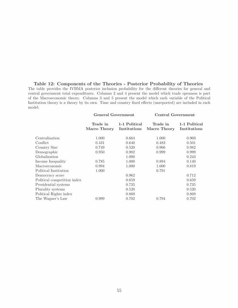
In this section we consider a sensitivity analysis of the baseline specification of theories.
Results are presented in Table 12. In particular, we do two things.
First, we merge the globalization and macroeconomic theories, as suggested by a large
21For centralization theory we use the percentage of central to general total government expenditure, forconflict theory we use the magnitude score of episode(s) of warfare involving that state in that year, forcountry size theory we use population, for demographic theory we use the percentage of people older than 64to the working-age population, for globalization theory we use trade openness, for income inequality theorywe use gross income gini inequality, for macroeconomic theory we use total central government debt, forpolitical institution theory we use the combined polity democracy score, and for the Wagner’s law theory weuse GDP per capita.
38
body of the literature. In order to be consistent with this we add trade openness into
macroeconomic theory. We find a decisive effect of the macroeconomic theory on general
government total expenditure, in contrast with the positive effect of the baseline model.
This is driven by trade openness, as suggested by the PIP of the included variable. The
effect of the macroeconomic theory on the central government expenditures remains decisive
and the inference of the variables remain consistent with our baseline model. For the rest
of the theories and variables, both the PIP, the posterior mean, and the posterior SD are
substantially the same with our baseline results. Our finding suggest that we get more
information by splitting globalization and macroeconomic theories without changing the
results of the rest theories.
Second, following Shelton (2007) we consider each component of the political institution
theory as its own theory. We let democracy score, political competition index, presidential
and plurality dummy, and political rights index to be theories on its own. In the baseline
model we find a strong effect of the political institution theory on general government total
expenditure and a positive effect on central government expenditure. Now, we find a strong
effect of democracy score and a positive effect of political rights on general government total
expenditure while we find a positive effect of political rights on central government total
expenditure. The results are consistent with Shelton (2007), but combining all variables
under one theory we additionally get the significant of the theory as a whole.
4.5.4 BMA and Classical Analysis
In addition to our IVBMA results, we present the top three models of IVBMA as well as the
largest model. We do so to provide the reader with the ability to compare results if one were
to engage in model selection. For completeness we also present least square BMA results
39
that do not take into account for endogeneity of the determinants.22 Results are presented
in Tables S16 and S17 of Supplementary Online Appendix.
The top three models yields posterior probability 0.031, 0.031 and 0.029 for the general
government total expenditure and 0.074, 0.068 and 0.041 for the central government total
expenditure, suggesting that r model space is not dominated by few models. Furthermore,
the largest model also known as “kitchen-sink” model, for both the general and the central
government expenditures, yields very different determinants for the government expenditure.
Nevertheless, given that the posterior model probability is approximately zero, this implies
that this model is not reliable for inference. Last but not least, there is a big difference
between our IVBMA results and the least squares BMA results, suggesting that ignoring the
endogeneity of the regressors can lead us to incorrect conclusions.
5 Conclusion
By now there exists a large literature on the size of government that proposed and tested
a wide range of alternative theories and hypotheses that determine the long run demand
and supply of government size. Yet, both theory and empirics have not provided convincing
answers about the determinants of government expenditure. This paper contributes to the
literature of government size by assessing the strength of the empirical relevance of those
theories by taking into account model uncertainty.
To address the issue of model uncertainty, we propose a novel BMA approach that
develops an Instrumental Variable Bayesian Model Averaging with priors defined in economic
theory space to account for the fact that the strength of several competing theories is
22For more information on the BMA estimation see Kass and Raftery (1995) andRaftery, Madigan, and Hoeting (1997).
40
simultaneously assessed using multiple proxy variables. In particular, our method introduces
BMA in linear models with endogenous regressors.
For general government we find decisive evidence for the demography theory, strong
evidence for the globalization and political institution theories, positive evidence for Wagner’s
law, centralization, income inequality and macroeconomic policy theories and weak evidence
for the country size and conflict theories. For the central government we find decisive
evidence for the macroeconomic policy, income inequality, and demography theories, positive
evidence for the centralization, political institution, globalization, and country size theories,
and weak evidence for Wagner’s law and conflict theories. These results are robust with
the variance decomposition and the channels of transmission analyses. Finally, we do not
find evidence for the explanation of Rodrik (1998), who suggests that the link between
government expenditure and globalization is based on the exposure to risk of the country.
Finally, the investigation of the formation of the components of government expenditure
suggests that different categories are affected by different theory. Hence, focusing only on
total expenditures can lead us to incomplete and misleading results. That said, there is a
a number of theories that affect both total and the various components. Particularly, the
demography theory affects both total and the various components of general government
and the demography, macroeconomic policy, and political institution theories affects both
total and the various components of central government.
41
Table 1: Posterior Probability of the TheoriesThe table provides the IVBMA posterior inclusion probability for the different theories for general and centralgovernment total expenditures and components. Time and country fixed effects (unreported) are includedin each model.
Table 2: Posterior Probability of the DeterminantsThe table provides the IVBMA posterior inclusion probability for the different determinants for general and central governmenttotal expenditures and components. Time and country fixed effects (unreported) are included in each model.
Table 3: Posterior Mean and Posterior Standard Deviation - General GovernmentThe table provides the IVBMA posterior mean and posterior standard deviation (in parenthesis) for the different determinants for general government total expenditureand components. Time and country fixed effects (unreported) are included in each model. ***, **, and * denote significance at 1%, 5%, and 10%, respectively.
Table 4: Posterior Mean and Posterior Standard Deviation - Central GovernmentThe table provides the IVBMA posterior mean and posterior standard deviation (in parenthesis) for the different determinants for general government total expenditureand components. Time and country fixed effects (unreported) are included in each model. ***, **, and * denote significance at 1%, 5%, and 10%, respectively.
Table 5: Variance DecompositionThe table presents the role of each theory in explaining the variation of the general and central governmenttotal expenditures and components, using the Balanced Variance Share (BVS) described in section 4.2.
Table 6: Channels of Transmission Analysis - Posterior Probability of Theories - Dropping TheoriesThe table provides the IVBMA posterior inclusion probability for the different theories for general and central government total expenditures when we exclude the various theories one-by-one.Time and country fixed effects (unreported) are included in each model.
Table 7: Channels of Transmission Analysis - Posterior Probability of Theories - Keeping TheoriesThe table provides the IVBMA posterior inclusion probability for the different theories for general and central government total expenditures when keeping the various theories one-by-one.Time and country fixed effects (unreported) are included in each model.
Table 8: Globalization - Posterior Probability of TheoriesThe table provides the IVBMA posterior inclusion probability for the different theories for general andcentral government total expenditures and components, taking into account the globalization as describedin Section 4.4.1. Time and country fixed effects (unreported) are included in each model.
Table 9: Income Inequality - Posterior Probability of TheoriesThe table provides the IVBMA posterior inclusion probability for the different theories for general and centralgovernment total expenditures and components, taking into account the heterogeneity in income inequality(Section 4.4.2). Time and country fixed effects (unreported) are included in each model.
Table 10: Parameter Heterogeneity - Posterior Probability of TheoriesThe table provides the IVBMA posterior inclusion probability for the different theories for general and centralgovernment total expenditures and components, taking into account the parameter heterogeneity (Section4.5.1). Time and country fixed effects (unreported) are included in each model.
Table 11: Prior of the Theories - Posterior Probability of TheoriesThe table provides the IVBMA posterior inclusion probability for the different theories for general andcentral government total expenditures, taking into account different priors. Time and country fixed effects(unreported) are included in each model.
General Government Central Government
One Variable Each Variable One Variable Each Variable
per Theory is a Theory per Theory is a Theory
Centralization 0.798 0.997 1.000 1.000Conflict 0.651 0.456 0.700 0.448Country Size 0.317 0.921Land area 0.857 0.318Population 0.825 0.998Demographic 1.000 1.000Dependency share < 15 0.732 0.065Dependency share > 64 1.000 1.000Urbanization 0.074 0.052Population growth 0.936 1.000Globalization 0.229 0.960 0.188 0.029Income Inequality 0.368 0.135 0.057 0.061Macroeconomic 0.939 0.750Central government debt 0.652 0.323FDI liabilities 0.458 0.938Inflation 0.028 0.019Political Institution 0.406 0.253Democracy score 0.516 0.331Political competition index 0.999 0.831Presidential systems 0.999 1.000Plurality systems 0.976 0.847Political Rights index 0.928 0.545The Wagner’s Law 0.999 0.869 0.897 0.420
54
Table 12: Components of the Theories - Posterior Probability of TheoriesThe table provides the IVBMA posterior inclusion probability for the different theories for general andcentral government total expenditures. Columns 2 and 4 present the model which trade openness is partof the Macroeconomic theory. Columns 3 and 5 present the model which each variable of the PoliticalInstitution theory is a theory by its own. Time and country fixed effects (unreported) are included in eachmodel.
General Government Central Government
Trade in 1-1 Political Trade in 1-1 Political
Macro Theory Institutions Macro Theory Institutions
Centralization 1.000 0.664 1.000 0.969Conflict 0.431 0.640 0.483 0.501Country Size 0.749 0.520 0.966 0.982Demographic 0.950 0.982 0.999 0.999Globalization 1.000 0.243Income Inequality 0.785 1.000 0.894 0.140Macroeconomic 0.994 1.000 1.000 0.819Political Institution 1.000 0.791Democracy score 0.962 0.712Political competition index 0.659 0.659Presidential systems 0.735 0.735Plurality systems 0.520 0.520Political Rights index 0.869 0.869The Wagner’s Law 0.999 0.702 0.794 0.702
55
Appendices
A1 Bayes Factors
In a general framework, incorporating model uncertainty involves considering a collection of
candidate models I, using the data D. Each model I consists of a collection of probability
distributions for the data D, pr(D|ψ), ψ ∈ ΨI where ΨI denotes the parameter space for
the parameters of model I and is a subset of the full parameter space Ψ.
By letting the model become an additional parameter to be assessed in the posterior,
we aim to calculate the posterior model probabilities given the data D. By Bayes’ rule
pr(I|D) =pr(D|I)pr(I)
∑
I′∈I pr(D|I ′)pr(I ′), (A1)
where pr(I), denotes the prior probability for model I ∈ I.
The integrated likelihood pr(D|I), is defined by
pr(D|I) =
∫
ΨI
pr(D|ψ)pr(ψ|I)dψ, (A2)
where pr(ψ|I) is the prior for ψ under model I, which by definition has all its mass on ΨI .
One possibility for pairwise comparison of models is offered by the Bayes factor (BF),
which is in most cases defined together with the posterior odds (Kass and Raftery (1995)).
The posterior odds of model I versus model I ′ is given by pr(I|D)pr(I′|D)
= pr(D|I)pr(D|I′)
pr(I)pr(I′)
, wherepr(D|I)pr(D|I′)
and pr(I)pr(I′)
denote the Bayes factor and the prior odds of I versus I ′, respectively.
When the integrated likelihood (A2) and thus, the BF can be computed directly, a
straightforward method for exploring the model space, Markov Chain Monte Carlo Model
Composition (MC3), was developed by Madigan and York (1995).
MC3 determines posterior model probabilities by generating a stochastic process that
moves through the model space I and has equilibrium distribution pr(I|D). Given the
current state I(s), MC3 proposes a new model I ′ according to a proposal distribution q(·|·),
56
calculates
α =pr(D|I ′)pr(I ′)q(I(s)|I ′)
pr(D|I(s))pr(I(s))q(I ′|I(s))
and sets I(s+1) = I ′ with probability minα, 1 otherwise setting I(s+1) = I(s).
It should be stressed that moving between models via the MC3 approach constitutes
a valid MCMC transition. This feature is critical in the development below, in that MC3
moves may be nested inside larger structures in a manner similar to Gibbs updates.
A2 Determining the CBF calculations
Here we outline the calculation of pr(D|Mr,β−r,K). Note that
pr(D|Mr,β−r,K) =
∫
ΛMr
pr(D|βr,β−r,K)pr(βr|Mr)dβr
Let Xr,Mrbe the submatrix of Xr associated with the variables in Mr and set Yr as above.
Then
∫
ΛMr
pr(D|βr,β−r,K)pr(βr|Mr)dβr ∝
∫
ΛMr
(2π)−|Mr|/2 exp
(
−1
2
[
−2βMrΩMr
βr + β′rΩMr
βr
]
)
dβr.
where ΩMr= KrrX
′
r,MrXr,Mr
+ I|Mr| and βMr= KrrΩ
−1Mr
X′
r,MrYr.
We can now see that the term in the integral is the canonical form of a Gaussian