66
Measuring the US Measuring the US Economy Economy Economic Indicators Economic Indicators
| Date post: | 14-Dec-2015 |
| Category: |
Documents |
| Upload: | jack-bradby |
| View: | 214 times |
| Download: | 0 times |

Measuring the US EconomyMeasuring the US Economy
Economic IndicatorsEconomic Indicators

Understanding the LingoUnderstanding the Lingo
Annualized RatesAnnualized Rates
Example: GDP Q3 (Final) = $11,814.9B (5.5%)Example: GDP Q3 (Final) = $11,814.9B (5.5%)
Q2: GDP = $2,914.38 B Q2: GDP = $2,914.38 B X 4 = $11,657.5 BQ3: GDP = $2,953.73 B Q3: GDP = $2,953.73 B X 4 = $11,814.9 B
($11,814.9 - $11,657.5) X 100 = 1.35% X4 = 5.5%$11,657.5

Understanding the LingoUnderstanding the Lingo
Annualized RatesAnnualized Rates
Supposed that prices increased by .3% during Supposed that prices increased by .3% during the month of November. the month of November.
The annualized inflation rate is .3%X12 = The annualized inflation rate is .3%X12 = 3.6%

Understanding the LingoUnderstanding the Lingo
Nominal (Current) Dollars vs. Real (Constant) Nominal (Current) Dollars vs. Real (Constant) DollarsDollarsExample: GDP(Q2) = $11,657.5Example: GDP(Q2) = $11,657.5
GDP(Q3) = $11,814.9T (5.5%)GDP(Q3) = $11,814.9T (5.5%)
CPI(Q2) = 111.2CPI(Q2) = 111.2
CPI(Q3) = 112.4 (4.3%)CPI(Q3) = 112.4 (4.3%)
Real GDP(Q2) = (11,657.5/111.2)*100 = $10,483.36Real GDP(Q2) = (11,657.5/111.2)*100 = $10,483.36
Real GDP(Q3) = (11,814.9/112.4)*100 = $10,511.47Real GDP(Q3) = (11,814.9/112.4)*100 = $10,511.47
($10,511.47 - $10,483.36)($10,511.47 - $10,483.36) X100 X 4 = 1.07% X100 X 4 = 1.07%
$10,483.36$10,483.36

Understanding the LingoUnderstanding the Lingo
Seasonally AdjustedSeasonally Adjusted
Retail Sales
250000
270000
290000
310000
330000
350000
370000
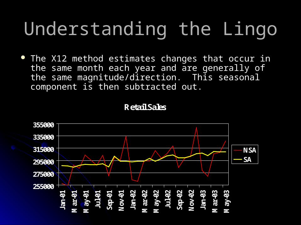
Understanding the LingoUnderstanding the Lingo The X12 method estimates changes that occur in the The X12 method estimates changes that occur in the
same month each year and are generally of the same same month each year and are generally of the same magnitude/direction. This seasonal component is magnitude/direction. This seasonal component is then subtracted out.then subtracted out.
Retail Sales
255000
275000
295000
315000
335000
355000
Jan-
01
Mar
-01
May
-01
Jul-
01
Sep-
01
Nov
-01
Jan-
02
Mar
-02
May
-02
Jul-
02
Sep-
02
Nov
-02
Jan-
03
Mar
-03
May
-03
NSASA

Understanding the LingoUnderstanding the Lingo
Moving AveragesMoving Averages
Example: Consider the following monthly Example: Consider the following monthly
Inflation Statistics (Monthly % Changes)Inflation Statistics (Monthly % Changes)
MayMay June June JulyJuly Aug.Aug. Sept.Sept. Oct.Oct. Nov.Nov. Dec.Dec.
.6.6 .3.3 -.1-.1 .1.1 .2.2 .6.6 .2.2 .2.2

Understanding the LingoUnderstanding the Lingo
Moving AveragesMoving Averages
A moving average takes out the volatility by averaging several A moving average takes out the volatility by averaging several observations. For example, a observations. For example, a MA(3) would average the current would average the current observation with the previous 2 observations.observation with the previous 2 observations.
MAMA MayMay June June JulyJuly Aug.Aug. Sept.Sept. Oct.Oct. Nov.Nov. Dec.Dec.
11 .6.6 .3.3 -.1-.1 .1.1 .2.2 .6.6 .2.2 .2.2
22 .45.45 .1.1 00 .15.15 .4.4 .4.4 .2.2
3 .27 .10 .07 .3 .33 .33
44 .3.3 .17.17 .2.2 .275.275 .3.3

Understanding the LingoUnderstanding the Lingo
RevisionsRevisions
ALL ECONOMIC DATA IS CONSTANTLY BEING REVISED!!!
Example: GDP is reported three timesExample: GDP is reported three times
Q3(Advance): 3.7%Q3(Advance): 3.7%
Q3 (Preliminary): 3.9%Q3 (Preliminary): 3.9%
Q3 (Final): 4.0%Q3 (Final): 4.0%

Understanding the LingoUnderstanding the Lingo
Consensus ForecastsConsensus Forecasts
Most of the news services construct consensus surveys by polling Most of the news services construct consensus surveys by polling economists for their predictions on key indicatorseconomists for their predictions on key indicators
GDPGDP ActualActual Consensus Consensus
AdvanceAdvance 3.7%3.7% 4.3%4.3%
PreliminaryPreliminary 3.9%3.9% 3.7%3.7%
FinalFinal 4.0%4.0% 3.9%3.9%

Understanding the LingoUnderstanding the Lingo BenchmarkingBenchmarking
Some indicators are reported relative to some Some indicators are reported relative to some benchmark.benchmark.
Example: Consumer Confidence in December was 102.3 Example: Consumer Confidence in December was 102.3 (1985 = 100)(1985 = 100)
Example: The CPI in November was 191.0 (1982-1984 = Example: The CPI in November was 191.0 (1982-1984 = 100)100)

Understanding the LingoUnderstanding the Lingo
The Business CycleThe Business CycleSince WWII, the US has Since WWII, the US has
experienced 10 Business experienced 10 Business cycles with the average cycles with the average recession lasting 10 recession lasting 10 months.months.
The most recent cycle was The most recent cycle was 2001:2001:
Peak (March 2001)Peak (March 2001) Trough (November Trough (November
2001)2001)

So Many Statistics….So Little So Many Statistics….So Little Time!Time!
The government releases over 50 The government releases over 50 statistics per month/quarter!! They can be statistics per month/quarter!! They can be roughly divided into 5 categoriesroughly divided into 5 categoriesConsumer SectorConsumer SectorBusiness SectorBusiness SectorPublic SectorPublic Sector InternationalInternationalPricesPrices

Major IndicatorsMajor Indicators
Consumer Sector (70% of Economic Activity)Consumer Sector (70% of Economic Activity) Retail Sales (Census Bureau) Consumer Credit (Federal Reserve) Personal Income and Spending (BEA) Employment Report (BLS) New Claims For Unemployment Insurance (Dept of Labor) Consumer Confidence/Sentiment (Conference Board/U. of
Michigan) Auto Sales (Dept. of Commerce)

Major IndicatorsMajor Indicators Business Sector(17% of Economic Activity)Business Sector(17% of Economic Activity)
Industrial Production (Federal Reserve)Industrial Production (Federal Reserve) Capacity Utilization (Federal Reserve)Capacity Utilization (Federal Reserve) ISM Index (Institute for Supply Management) Durable Goods Orders (Census Bureau) Factory Orders (Census Bureau)Factory Orders (Census Bureau)
Housing Starts (Census Bureau) New/Existing Home Sales (Nat. Assoc. of Realtors/Census
Bureau) MBA Mortgage Applications (Mortgage Bankers Assoc.)
Business inventories (Census Bureau)Business inventories (Census Bureau)

Major IndicatorsMajor Indicators
Public Sector(19% of Economic Activity)Public Sector(19% of Economic Activity) Construction Spending (Census)Construction Spending (Census) Federal Budget Report (Treasury Dept)
International Sector (-6% of Economic Activity) Net Exports (Bureau of Economic Analysis) Current Account (Bureau of Economic Analysis)
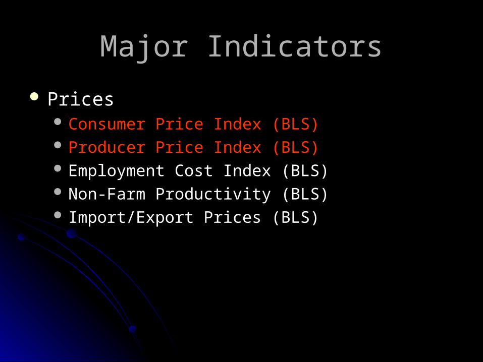
Major IndicatorsMajor Indicators
PricesPrices Consumer Price Index (BLS) Producer Price Index (BLS) Employment Cost Index (BLS) Non-Farm Productivity (BLS) Import/Export Prices (BLS)

Criteria For “Good” IndicatorsCriteria For “Good” Indicators
Accuracy: Accuracy: Most economic data is compiled through surveys – Most economic data is compiled through surveys –
larger survey pools are more accurate.larger survey pools are more accurate. To measure consumer confidence, the conference board To measure consumer confidence, the conference board
polls 5,000 households per month.polls 5,000 households per month. To measure prices, the bureau of labor statistics polls 28,000 To measure prices, the bureau of labor statistics polls 28,000
retail outlets per month! (on 80,000 products)retail outlets per month! (on 80,000 products) Some statistics are subject to large revisions.Some statistics are subject to large revisions.
Housing starts are rarely revised while the monthly Housing starts are rarely revised while the monthly construction spending report often gets substantial revisionsconstruction spending report often gets substantial revisions

Criteria For “Good” IndicatorsCriteria For “Good” Indicators
TimelinessTimelinessThe BLS employment situation report comes The BLS employment situation report comes out a week after the end of the month, while out a week after the end of the month, while consumer credit is reported on a two month consumer credit is reported on a two month delay.delay.

Predictive AbilityPredictive Ability
Blue Arrow = PeakBlue Arrow = Peak Red Arrow = TroughRed Arrow = Trough

Predictive AbilityPredictive Ability
Blue Arrow = PeakBlue Arrow = Peak Red Arrow = TroughRed Arrow = Trough

Predictive AbilityPredictive Ability
Blue Arrow = PeakBlue Arrow = Peak Red Arrow = TroughRed Arrow = Trough

Criteria For “Good” IndicatorsCriteria For “Good” Indicators
Business Cycle StageBusiness Cycle StageDuring recessions, we’re looking for signs of During recessions, we’re looking for signs of
recoveryrecoveryHousing StartsHousing StartsAuto SalesAuto SalesEmploymentEmployment
During expansions we tend to be more During expansions we tend to be more concerned with inflationconcerned with inflationCPICPIEmployment cost indexEmployment cost index
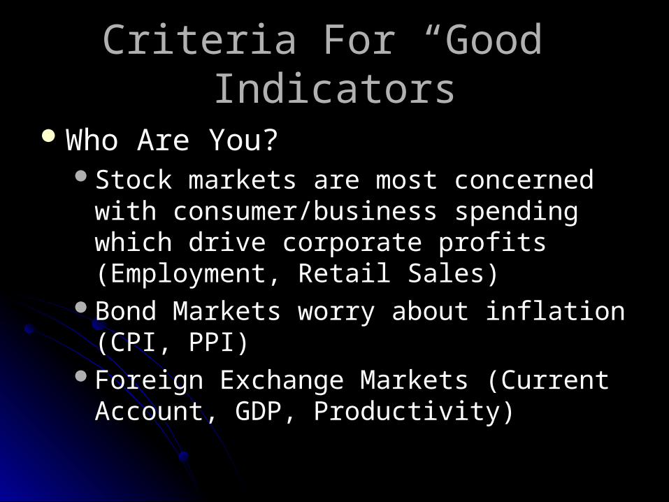
Criteria For “Good” IndicatorsCriteria For “Good” Indicators
Who Are You?Who Are You?Stock markets are most concerned with Stock markets are most concerned with
consumer/business spending which drive consumer/business spending which drive corporate profits (Employment, Retail Sales)corporate profits (Employment, Retail Sales)
Bond Markets worry about inflation (CPI, PPI)Bond Markets worry about inflation (CPI, PPI)Foreign Exchange Markets (Current Account, Foreign Exchange Markets (Current Account,
GDP, Productivity)GDP, Productivity)

A ShortcutA Shortcut
Index of Leading Indicators (Conference Board)Index of Leading Indicators (Conference Board) Average Hourly Workweek in Manufacturing (19.7%)Average Hourly Workweek in Manufacturing (19.7%) Weekly Unemployment Claims (2.5%)Weekly Unemployment Claims (2.5%) Manufacturers’ New Orders – Consumer Goods (5.9%)Manufacturers’ New Orders – Consumer Goods (5.9%) Manufacturers’ New Orders – Capital Goods (1.5%)Manufacturers’ New Orders – Capital Goods (1.5%) Vendor Performance (Delivery Time Index) (2.9%)Vendor Performance (Delivery Time Index) (2.9%) Building Permits for New Homes (2%)Building Permits for New Homes (2%) Index of Consumer Expectations (1.9%)Index of Consumer Expectations (1.9%)
S&P Index (2.9%)S&P Index (2.9%) Real (inflation adjusted) M2 Money Supply (27.7%)Real (inflation adjusted) M2 Money Supply (27.7%) Interest Spread Between 10 Yr. Bonds & Fed Funds Rate (33%)Interest Spread Between 10 Yr. Bonds & Fed Funds Rate (33%)

Index of Leading IndicatorsIndex of Leading Indicators
Blue Arrow = PeakBlue Arrow = Peak Red Arrow = TroughRed Arrow = Trough

The Most Influential U.S. The Most Influential U.S. Economic IndicatorsEconomic Indicators

The Big One: EmploymentThe Big One: Employment
What is it: Total (Non-Farm) Employment, Unemployment : Total (Non-Farm) Employment, Unemployment Rate, Average Duration, etc…..Are people Rate, Average Duration, etc…..Are people working? working?
Release Time: 8:00AM, the first Friday of the month : 8:00AM, the first Friday of the month following the coverage month following the coverage month
Frequency: Monthly: Monthly
Source: Bureau of Labor Statistics: Bureau of Labor Statistics
Revisions: Frequent Revisions…sometimes major!: Frequent Revisions…sometimes major!

The Household SurveyThe Household Survey
Each month, the BLS contacts 60,000 Each month, the BLS contacts 60,000 households (95% response rate) and places households (95% response rate) and places each in one of four categorieseach in one of four categories::
A. Under 16 or institutionalized (or military)
B. Choose not to work: Not in Labor Force
C. Choose to work and are working: Employed
D. Choose to work, but can’t find a job: Unemployed
Unemployment Rate = D/(D+C)

Household SurveyHousehold Survey US Population: 290MUS Population: 290M Civilian Population: 220MCivilian Population: 220M Labor Force: 147MLabor Force: 147M Employment: 139MEmployment: 139M Unemployment: 8MUnemployment: 8M
Participation RateParticipation Rate (147M/220M)*100 = 66%(147M/220M)*100 = 66%
Employment RatioEmployment Ratio
(138M/220M)*100 = 62%(138M/220M)*100 = 62%
Unemployment RateUnemployment Rate
(8M/147M)*100 = 5.4%(8M/147M)*100 = 5.4%
UR = 1 – (ER/PR)UR = 1 – (ER/PR)

US Participation RateUS Participation Rate

US Participation RateUS Participation Rate

Establishment (Payroll) SurveyEstablishment (Payroll) Survey
Each month, the BLS contacts 400,000 Each month, the BLS contacts 400,000 firms!! (60% - 70%) response rate. Each firms!! (60% - 70%) response rate. Each firm is asked to report total employment.firm is asked to report total employment.
Employment: 131M??Employment: 131M??
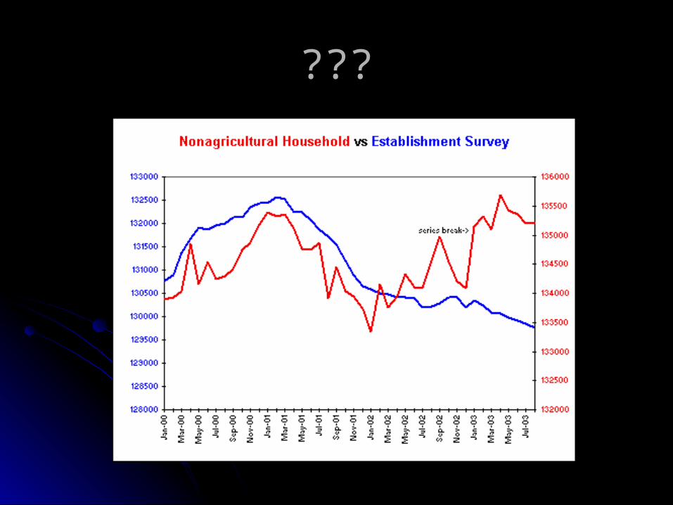
??????

The US Labor MarketThe US Labor Market
Labor markets are difficult to characterize Labor markets are difficult to characterize because they are always in motion…..because they are always in motion…..
NOT IN LABOR FORCE
EMPLOYED
UNEMPLOYED
Average Turnover is around 2.5 Million people per Month!!

DurationDuration Most unemployment spells Most unemployment spells
in the US are short.in the US are short.
<5 Wks: 2.9m<5 Wks: 2.9m 5-15 Wks: 2.2m5-15 Wks: 2.2m+ >15 Wks: 2.9m+ >15 Wks: 2.9m
Total: 8.0mTotal: 8.0m
Average duration in the US Average duration in the US is approx. 19wksis approx. 19wks
Median: 9wksMedian: 9wks
Average DurationAverage Duration In 1 year, how many people In 1 year, how many people
are unemployed for 5 wks?are unemployed for 5 wks?(52/5)*2.9M = 30.1M(52/5)*2.9M = 30.1M
How many people are How many people are unemployed for 10 wks?unemployed for 10 wks?(52/10)*2.2M = 11.4M(52/10)*2.2M = 11.4M
For 20 wks?For 20 wks?++(52/20)*2.9M = 7.5M(52/20)*2.9M = 7.5M Total 49MTotal 49M
AD = (30.1/49)*(5wks) + AD = (30.1/49)*(5wks) + (11.4/49)*(10wks) + (11.4/49)*(10wks) + (7.5/49)*(20wks) =(7.5/49)*(20wks) = 8.5wks

Unemployment DurationUnemployment Duration

Unemployment DurationUnemployment Duration

What’s “Normal” in the Labor What’s “Normal” in the Labor Market?Market?
Frictional Unemployment: Currently unemployed, but in Frictional Unemployment: Currently unemployed, but in the process of getting a job (i.e., short term the process of getting a job (i.e., short term unemployment): unemployment): 3.5%3.5%
+ + Structural Unemployment (chronic unemployment): 1.5%Structural Unemployment (chronic unemployment): 1.5%
““Natural Rate of Unemployment”: Natural Rate of Unemployment”: 5%
Given the current unemployment rate of 5.4%, we Given the current unemployment rate of 5.4%, we currently have a currently have a cyclical unemployment rate of .4%of .4%

US Unemployment Rate: 1990-2002US Unemployment Rate: 1990-2002
0123456789

Is the “Natural Rate” Growing?Is the “Natural Rate” Growing?
0
2
4
6
8
10
12
1948
1951
1954
1957
1960
1963
1966
1969
1972
1975
1978
1981
1984
1987
1990
1993
1996
1999
2002

The cost of unemploymentThe cost of unemployment
““Capacity Output” of an economy is the level of Capacity Output” of an economy is the level of output associated with full employment (i.e., output associated with full employment (i.e., unemployment is at the natural rate)unemployment is at the natural rate) The “output gap” is the difference between capacity The “output gap” is the difference between capacity
output and actual outputoutput and actual output Okun’s law states that every 1% increase in cyclical Okun’s law states that every 1% increase in cyclical
unemployment increases the output gap by 2.5%. unemployment increases the output gap by 2.5%. Therefore, our current .4% cyclical unemployment Therefore, our current .4% cyclical unemployment
rate implies an output gap of 1% GPD ( Roughly rate implies an output gap of 1% GPD ( Roughly $110B! )$110B! )

GDP (Gross Domestic Product)GDP (Gross Domestic Product)
What is it: Current dollar value of all goods and service produced in the : Current dollar value of all goods and service produced in the US US
Release Time: 8:30AM, The final week of the month : 8:30AM, The final week of the month following the covered quarter (each quarter has following the covered quarter (each quarter has
three three estimates: Advance, Preliminary, Final) estimates: Advance, Preliminary, Final)
Frequency: Quarterly: Quarterly
Source: Bureau of Economic Analysis: Bureau of Economic Analysis
Revisions: They usually get it right by the final revision.: They usually get it right by the final revision.

Calculating GDPCalculating GDP
If our economy was horizontally oriented If our economy was horizontally oriented (i.e. everyone produces final goods) (i.e. everyone produces final goods) economy, calculating GDP would be easy: economy, calculating GDP would be easy:
GDP = Price*Quantity (Added up over all goods)GDP = Price*Quantity (Added up over all goods) Our economy is vertically oriented (some Our economy is vertically oriented (some
manufacturers produce manufacturers produce intermediate goods). Therefore, we must avoid double Therefore, we must avoid double counting.counting.
Each manufacturer reports output on a Each manufacturer reports output on a value added basis

NNational ational IIncome and ncome and PProduct roduct AAccountsccounts
GDP (2003)GDP (2003)Consumer Consumer Goods: $7,752.2BGoods: $7,752.2B
InvestmentInvestment Goods: $1,667.5BGoods: $1,667.5B
GovernmentGovernmentExpenditures: $2,055.7BExpenditures: $2,055.7B
Net Exports: -$491.5BNet Exports: -$491.5B $10,983.9
Income (2003)Income (2003)
GDP: $10,983.9GDP: $10,983.9
- - Net Factor Payments: $37.9Net Factor Payments: $37.9GNP: $10,946.0GNP: $10,946.0
- Depreciation $1,370.1Depreciation $1,370.1NNP: $9,575.9NNP: $9,575.9
- Indirect Taxes: $834.4Indirect Taxes: $834.4National Income: National Income: $8741.5

NNational ational IIncome and ncome and PProduct roduct AAccountsccounts
Income (2003)Income (2003)
GDP: $10,983.9GDP: $10,983.9
- - Net Factor Payments: $37.9Net Factor Payments: $37.9GNP: $10,946.0GNP: $10,946.0
- Depreciation $1,370.1Depreciation $1,370.1NNP: $9,575.9NNP: $9,575.9
- Indirect Taxes: $834.4Indirect Taxes: $834.4National Income: National Income: $8741.5
Income (2003)Income (2003)
Wages: $6,039.5Wages: $6,039.5
Proprietor’s Income: $774.6Proprietor’s Income: $774.6
Rental Income: $127.9 Rental Income: $127.9
Corporate Profits: $1,294.2Corporate Profits: $1,294.2
Interest: $546.9Interest: $546.9National Income: National Income: $8,783.1 Statistical Discrepancy: Statistical Discrepancy: 41.6B
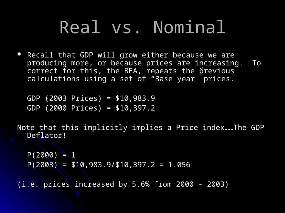
Real vs. NominalReal vs. Nominal Recall that GDP will grow either because we are producing more, or Recall that GDP will grow either because we are producing more, or
because prices are increasing. To correct for this, the BEA, repeats because prices are increasing. To correct for this, the BEA, repeats the previous calculations using a set of “Base year” prices.the previous calculations using a set of “Base year” prices.
GDP (2003 Prices) = $10,983.9GDP (2003 Prices) = $10,983.9GDP (2000 Prices) = $10,397.2GDP (2000 Prices) = $10,397.2
Note that this implicitly implies a Price index……The GDP Deflator!Note that this implicitly implies a Price index……The GDP Deflator!
P(2000) = 1P(2000) = 1P(2003) = $10,983.9/$10,397.2 = 1.056P(2003) = $10,983.9/$10,397.2 = 1.056
(i.e. prices increased by 5.6% from 2000 – 2003)(i.e. prices increased by 5.6% from 2000 – 2003)

GDP FactsGDP Facts
GDP in 2004 is $11,649.3 Billion while GDP in 1950 GDP in 2004 is $11,649.3 Billion while GDP in 1950 was $275.7 Billion. (an increase of 4200%). was $275.7 Billion. (an increase of 4200%).
Real GDP (2000 $s) in 2004 was $10,788.9 Billion Real GDP (2000 $s) in 2004 was $10,788.9 Billion while Real GDP in 1950 was $1,777.5 Billion (A while Real GDP in 1950 was $1,777.5 Billion (A 600% increase)600% increase)
Real GDP per capita in 2003 is $36,911 compared Real GDP per capita in 2003 is $36,911 compared to $10,736 in 1950 ( a 350% increase). to $10,736 in 1950 ( a 350% increase).
Median real income in 2003 is approximately Median real income in 2003 is approximately $24,000 while median real income in 1950 was $24,000 while median real income in 1950 was approximately $8,000 (a 300% increase)approximately $8,000 (a 300% increase)

CPI (Consumer Price Index)CPI (Consumer Price Index)
What is it: The “Average” Price of Consumer Goods in the US: The “Average” Price of Consumer Goods in the US
Release Time: 8:30AM, The second or third week following the : 8:30AM, The second or third week following the covered monthcovered month
Frequency: Monthly: Monthly
Source: Bureau of Labor Statistics: Bureau of Labor Statistics
Revisions: No Revisions except for an annual correction done in : No Revisions except for an annual correction done in February.February.

Fixed Weight IndicesFixed Weight Indices
A price index is meant to capture the average price of A price index is meant to capture the average price of goods and services in the economy. Therefore, any goods and services in the economy. Therefore, any price index should be a weighted average of all (or at price index should be a weighted average of all (or at least, most) prices in the economy.least, most) prices in the economy.
With any fixed weight index, the weights used in the With any fixed weight index, the weights used in the index are chosen ex ante and remain fixed over time index are chosen ex ante and remain fixed over time (hence, the name (hence, the name fixedfixed weight index). weight index).
Think of the a fixed weight index as simply defining a Think of the a fixed weight index as simply defining a “basket” of goods. The value of that index is the cost of “basket” of goods. The value of that index is the cost of that basket.that basket.

Example: A Fixed Weight IndexExample: A Fixed Weight Index Suppose that in 2002, Apples Suppose that in 2002, Apples
cost $3 and Oranges cost $5. cost $3 and Oranges cost $5. In 2003, Apples cost $4 (a In 2003, Apples cost $4 (a 30% increase) and oranges 30% increase) and oranges cost $6. (20% increase)cost $6. (20% increase)
Let’s define the price index as Let’s define the price index as .5( Apples) + .5(Oranges).5( Apples) + .5(Oranges)
Usually, prices are in Usually, prices are in represented in terms of a represented in terms of a “base year”. This is done by “base year”. This is done by dividing every year by the dividing every year by the base year pricebase year price
P(2002) = .5($3) + .5($5)P(2002) = .5($3) + .5($5) = $4.= $4.
P(2003) = .5($4) + .5($6) P(2003) = .5($4) + .5($6) = $5= $5
P(2002) = 1 (or 100)P(2002) = 1 (or 100)P(2003) = $5/$4 = 1.25 (or P(2003) = $5/$4 = 1.25 (or
125)125)

The Consumer Price IndexThe Consumer Price Index
40%
5%17%
6%
6%
5%
1%
4%
16%Housing
Apparel
Transportation
Medical
Recreation
Education &CommunicationTobacco & SmokingProductsPersonal Care
Food & Beverage

The Consumer Price IndexThe Consumer Price Index
The inflation rate is just the percentage change The inflation rate is just the percentage change in the CPI. in the CPI.
The “core inflation rate” is the the percentage The “core inflation rate” is the the percentage change in the CPI less energy and food prices change in the CPI less energy and food prices (known to be extremely volatile)(known to be extremely volatile)
The producer price index (PPI) is the corporate The producer price index (PPI) is the corporate analogue to the CPIanalogue to the CPI

Problems with the CPIProblems with the CPI
A formal commission A formal commission headed by Stanford headed by Stanford economist Michael economist Michael Boskin in 1996 Boskin in 1996 determined that the determined that the CPI overestimated by CPI overestimated by as much as 2.4% per as much as 2.4% per yearyear
Formula Bias: .3-.4%Formula Bias: .3-.4%
Substitution Substitution Bias: .2-.4%Bias: .2-.4%
Outlet Bias: .1-.3%Outlet Bias: .1-.3%
New Products: .2-.7%New Products: .2-.7%
Quality Bias: .2-.6%Quality Bias: .2-.6%
Total: 1 - 2.4%Total: 1 - 2.4%
Variable Weight IndicesVariable Weight Indices
Variable weight indices correct for the substitution bias of Variable weight indices correct for the substitution bias of the CPI by allowing the weights to vary over time.the CPI by allowing the weights to vary over time.
The GDP Deflator (or, more commonly, the deflator) The GDP Deflator (or, more commonly, the deflator) uses actual production of each commodity as a fraction uses actual production of each commodity as a fraction of total GDP for the weights. Therefore as production of total GDP for the weights. Therefore as production (and, hence, consumption) of a commodity rises, so (and, hence, consumption) of a commodity rises, so does its weight in the deflator.does its weight in the deflator.

Chain WeightingChain Weighting
During periods of large relative price During periods of large relative price changes, the choice of base year is critical changes, the choice of base year is critical for determining real growth and the for determining real growth and the behavior of prices.behavior of prices.
Chain weighting is a process by which a Chain weighting is a process by which a range of years is chosen for the “base range of years is chosen for the “base year” and that range moves over time.year” and that range moves over time.

ProductivityProductivity
What is it: A Measure of Efficiency in the Production Sector: A Measure of Efficiency in the Production Sector
Release Time: 8:30AM, Around five weeks following the covered : 8:30AM, Around five weeks following the covered quarter quarter
Frequency: Quarterly: Quarterly
Source: Bureau of Labor Statistics: Bureau of Labor Statistics
Revisions: Can be substantial….this depends on revisions to both : Can be substantial….this depends on revisions to both GDP and EmploymentGDP and Employment

Calculating ProductivityCalculating Productivity
Step #1: Take real GDP and subtract out Step #1: Take real GDP and subtract out government output and farm outputgovernment output and farm output
$10,397.2 - $2,079.44 = $8,317.8$10,397.2 - $2,079.44 = $8,317.8
Step #2: Divide by Total Labor Hours (in the Employment Situation Report)Step #2: Divide by Total Labor Hours (in the Employment Situation Report) (Employment * Average Hours *52 = Total Hours)(Employment * Average Hours *52 = Total Hours)
$8,317.8/244.3 = $34/hr.$8,317.8/244.3 = $34/hr.
Step #3: Productivity is benchmarked relative to a “base year” Step #3: Productivity is benchmarked relative to a “base year”
Suppose that Output/hr in 1992 was equal to $28.hr, then Suppose that Output/hr in 1992 was equal to $28.hr, then
Prod(1992) = 100Prod(1992) = 100Prod(2003) = 100*(34/28) = 121.4Prod(2003) = 100*(34/28) = 121.4

Y = real outputN= labor hoursK=capital input
Y/N = Labor Productivity y – n = Labor Productivity growth (lower case letters = compound annual average rates of growth)
Y = A KβN1-β = Production function (Cobb Douglas)
A = Y/(KβN1-β) = Multifactor Productivity a = y – βk – (1-β)n = Growth Rate of MFP
y - n = a + β (k - n) = Growth rate of labor productivity
Labor and Multifactor Productivity Labor and Multifactor Productivity Growth FormulasGrowth Formulas

Labor Productivity, United States, Labor Productivity, United States, 1919-20001919-2000
1919-19291919-1929 2.272.27
1929-19411929-1941 2.352.35
1941-19481941-1948 1.711.71
1948-19731948-1973 2.882.88
1973-19891973-1989 1.331.33
1989-20001989-2000 1.971.97
1973-19951973-1995 1.401.40
1995-20001995-2000 2.432.43Sources: 1919-48: Kendrick (1961), Table A-23.Sources: 1919-48: Kendrick (1961), Table A-23.
1948-2000: Bureau of Labor Statistics: www.bls.gov1948-2000: Bureau of Labor Statistics: www.bls.gov

MFPMFPUnited States, 1919-2000United States, 1919-2000
1919-19291919-1929 2.022.021929-19411929-1941 2.312.311941-19481941-1948 1.291.291948-19731948-1973 1.901.901973-19891973-1989 .34 .341989-20001989-2000 .78 .78
1973-19951973-1995 .38 .381995-20001995-2000 1.141.14
Sources: 1919-48: Field (2003); Kendrick (1961)Sources: 1919-48: Field (2003); Kendrick (1961) 1948-2000: Bureau of Labor Statistics: www.bls.gov1948-2000: Bureau of Labor Statistics: www.bls.gov

Consumer ConfidenceConsumer Confidence
What is it: A Measure of how consumers feel about the : A Measure of how consumers feel about the economy economy
Release Time: 10:00AM, The last Tuesday of the month : 10:00AM, The last Tuesday of the month being surveyed being surveyed
Frequency: Monthly: Monthly
Source: The Conference Board: The Conference Board
Revisions: Minor : Minor

Measuring Consumer ConfidenceMeasuring Consumer Confidence
The board surveys 5,000 households/month and asks the The board surveys 5,000 households/month and asks the
following questions:following questions: 1) How would you rate the present general business conditions in 1) How would you rate the present general business conditions in your area? Good, Normal, or Bad.your area? Good, Normal, or Bad.
2) How about six months from now? Better, Same, Worse.2) How about six months from now? Better, Same, Worse.
3) What would you say about available jobs in your area? Plenty, 3) What would you say about available jobs in your area? Plenty, not so many, hard to get. not so many, hard to get.
4) What about six months from now? Better, Same, Worse.4) What about six months from now? Better, Same, Worse.
5) What would you guess your family income to be six months from 5) What would you guess your family income to be six months from now? Higher, same, lower.now? Higher, same, lower.

Measuring Consumer ConfidenceMeasuring Consumer Confidence
The board surveys 5,000 households/month and asks the The board surveys 5,000 households/month and asks the
following questions:following questions: Step #1: For each question, the “Neutral” Response is thrown out. For each question, the “Neutral” Response is thrown out.
Step #2: The responses are transformed into a percentage The responses are transformed into a percentage
Relative Response = Positive/(Positive + Negative)Relative Response = Positive/(Positive + Negative)
Step #3: The Benchmark is relative to 1985. The Benchmark is relative to 1985.
Benchmarked Answer = Rel. Response (Current)/Relative Response(1985)Benchmarked Answer = Rel. Response (Current)/Relative Response(1985)
Step #4: Average over the 5 questions: Average over the 5 questions

Example: Consumer ConfidenceExample: Consumer Confidence
QuestionQuestion PositivePositive NeutralNeutral NegativeNegative RelativeRelative BenchmarkedBenchmarked
#1#1 3,0003,000 1,0001,000 1,0001,000 .75 .75 1.071.07
#2#2 2,0002,000 500500 2,5002,500 .44.44 1.101.10
#3#3 2,9002,900 100100 2,0002,000 .59.59 1.181.18
#4#4 1,5751,575 1,5751,575 1,8501,850 .46.46 0.760.76
#5#5 1,0001,000 1,0001,000 3,0003,000 .25.25 0.630.63
AverageAverage 20952095 835835 20702070 .50.50 .948*100 = 94.8
Relative Values for 1985 are: .70, .40, .50, .60, .40 Relative Values for 1985 are: .70, .40, .50, .60, .40 (Average = .52)(Average = .52)

The Bottom LineThe Bottom Line
Each statistic has its strengths and Each statistic has its strengths and weaknesses. weaknesses.
Rarely will all the indicators “agree” with Rarely will all the indicators “agree” with one another. one another.
Each indicator must be looked at in the Each indicator must be looked at in the context of “the big picture”. context of “the big picture”.


