Measuring Welfare for Small but Vulnerable Groups: Poverty and Disability in Uganda Johannes G. Hoogeveen 1 World Bank When vulnerable population groups are numerically small — as is often the case — obtaining representative welfare estimates from non-purposive sample surveys becomes an issue. Building on a method developed by Elbers et al., it is shown how, for census years, estimates of consumption poverty for small vulnerable populations can be derived by combining sample survey and population census information. The approach is illustrated for Uganda, for which poverty amongst households with disabled heads is determined. 1. Introduction Absence of statistically precise poverty information affects many vulnerable groups. Poverty statistics for people with disabilities, for child-headed households, for young widows, for those working in hazardous occupations or for small ethnic minorities, are virtually non-existent. One reason for this paucity of information is that it is hard to obtain representative statistics for small population groups. National sample surveys may collect some information, but typically the number of observations is too small for welfare estimates to be precise. Stratification allows, at least in theory, to identify less populous population groups in sufficiently large q The author 2005. Published by Oxford University Press on behalf of the Centre for the Study of African Economies. All rights reserved. For permissions, please email: [email protected]1 The findings, interpretations and conclusions expressed in this paper are entirely those of the author. They do not necessarily represent the view of the World Bank, its Executive Directors or the countries they represent. The author would like to thank Jenny Lanjouw, Peter Lanjouw, Johan Mistiaen, Daniel Mons, Roy van der Weide and participants to research seminars at the World Bank, in Dar es Salaam and the Tinbergen Institute Amsterdam for useful comments, suggestions and other types of assistance. All remaining errors are entirely mine. Financial support by the Bank Netherlands Partnership Program is gratefully acknowledged. JOURNAL OF AFRICAN ECONOMIES,VOLUME 14, NUMBER 4, PP . 603–631 doi:10.1093/jae/eji020 online date 1 August 2005
Transcript
Measuring Welfare for Small but Vulnerable Groups:Poverty and Disability in Uganda
Johannes G. Hoogeveen1
World Bank
When vulnerable population groups are numerically small — as is oftenthe case — obtaining representative welfare estimates from non-purposivesample surveys becomes an issue. Building on a method developed byElbers et al., it is shown how, for census years, estimates of consumptionpoverty for small vulnerable populations can be derived by combiningsample survey and population census information. The approach isillustrated for Uganda, for which poverty amongst households withdisabled heads is determined.
1. Introduction
Absence of statistically precise poverty information affects manyvulnerable groups. Poverty statistics for people with disabilities, forchild-headed households, for young widows, for those working inhazardous occupations or for small ethnic minorities, are virtuallynon-existent. One reason for this paucity of information is that it ishard to obtain representative statistics for small population groups.National sample surveys may collect some information, buttypically the number of observations is too small for welfareestimates to be precise. Stratification allows, at least in theory, toidentify less populous population groups in sufficiently large
q The author 2005. Published by Oxford University Press on behalf ofthe Centre for the Study of African Economies. All rights reserved.For permissions, please email: [email protected]
1 The findings, interpretations and conclusions expressed in this paper are entirelythose of the author. They do not necessarily represent the view of theWorld Bank,its Executive Directors or the countries they represent. The author would like tothank Jenny Lanjouw, Peter Lanjouw, Johan Mistiaen, Daniel Mons, Roy van derWeide and participants to research seminars at the World Bank, in Dar es Salaamand the Tinbergen Institute Amsterdam for useful comments, suggestions andother types of assistance. All remaining errors are entirely mine. Financialsupport by the Bank Netherlands Partnership Program is gratefullyacknowledged.
JOURNAL OF AFRICAN ECONOMIES, VOLUME 14, NUMBER 4, PP. 603–631doi:10.1093/jae/eji020 online date 1 August 2005
numbers to provide representative estimates. But in practicestratification of small target populations tends to be dropped infavour of other concerns. Consequently, sample surveys— the mainsource of information on household welfare for developingcountries — provide little (or statistically imprecise) informationfor small target populations. This leads to a statistical invisibility ofthe welfare conditions of many less populous groups.
By reporting on each individual in a country, censuses provideprecise information for even the smallest population group, butonly collect information about non-consumption dimensions ofwelfare, such as household size, educational attainment or access toclean water. Consequently information about, say, the educationalattainment of disabled people is available, but a comparison of theincidence of consumption poverty amongst people with disabilitiesand the general population cannot be made. In this paper it isshown how small area welfare estimation techniques whichcombine consumption-based welfare information from nationalsample surveys with welfare correlates from censuses can be usedto generate consumption poverty estimates for small targetpopulations.2
There are various approaches to small area estimation (forsurveys, see Ghosh and Rao, 1994; Rao, 1999). A method thatrecently has attracted considerable attention — for its ability toarrive at welfare estimates and their standard errors — is describedin Elbers et al. (2003). It has, to date, only been used to derive welfareestimates for small administrative areas. In this paper the samemethod is employed to arrive at welfare estimates for small targetpopulations. If these target populations are characterised by limitedresilience to avoid poverty and few opportunities to escapechronic poverty, they are often referred to as vulnerable groups.3
The small vulnerable group on which this paper focuses are peoplewith disabilities.
2 In the literature the terms ‘small area welfare estimation’ and ‘poverty mapping’are used interchangeably to refer to welfare estimates derived for small targetpopulations.
3 The term ‘vulnerable group’ is used even if risk and its consequences forfuture well-being (that is vulnerability) are less of a concern. Often, however,there is a considerable overlap between vulnerable groups and vulnerability, aslimited resilience and opportunities will make vulnerable groups especiallyliable to further impoverishment in risky environments. For a more elaboratediscussion of the distinction between vulnerability and vulnerable groups, seeHoogeveen et al. (2004) and the introduction to this volume.
604 J.G. Hoogevenn
The likelihood that disabled people experience poverty is greaterthan that for the population at large. There are many reasons forthis. Exclusion and discrimination, unequal access to food, healthcare and education, and reduced capabilities for work all contributeto reduce opportunities for disabled people and their consumption-generating capabilities. Despite the obvious relationship betweendisability and poverty, there is little to no reliable statisticalinformation to substantiate this point (Metts, 2000; Yeo andMoore, 2003).
Using the Elbers et al. (2003) method, poverty estimates arederived, for 1992, for urban Ugandan households with a disabledhead. The estimates show that 27% of the urban dwellers are poorand that poverty amongst those who live in a household with adisabled head is much higher, 43%. This latter estimate is argued tobe a lower bound. The standard errors of the estimates of povertyincidence amongst people with disabilities are small and lower thanthe standard errors associated to the poverty estimates obtainedfrom the national household survey. Further disaggregation istherefore feasible and regional estimates of poverty amongst(non)disabled male and female headed households are presentedas well.
The paper is organised as follows. In the next section an overviewof the available information on poverty and disability in Uganda isprovided. This information comprises qualitative data on povertyamongst people with disabilities and quantitative information onhousehold characteristics of disabled people. In section three theestimation strategy to arrive at poverty estimates is outlined and itis explained how the precision of the census-based welfareestimates depends on the size of the target population. Sectionfour briefly describes the data after which section five presentswelfare estimates for urban households with a disabled head.Section six discusses for which administrative level precise povertystatistics for people with disabilities can be generated, and presentsregional poverty predictions by gender and disability status. Sectionseven discusses a key assumption underlying the approach: that theprediction model derived for the population as a whole is unbiasedfor the sub-group of disabled people. It is argued that because themodels used for consumption prediction comprise mostly con-sumption correlates rather than structural variables, prediction biasis less of an issue. The section suggests two approaches to explore
Poverty and Disability in Uganda 605
the presence of such bias and argues that in the case of disabilityunobserved household characteristics are likely to lead to anunderestimation of poverty. A summary of the findings concludesthe paper.
2. Poverty and Disability in Uganda
That Uganda’s disabled are deprived is demonstrated in detail byqualitative research. Uganda’s Participatory Poverty Assessment(Republic of Uganda, 2002), which operated in 60 sites and 12 ofUganda’s 56 districts, provides numerous illustrations of thehardships faced by people with disabilities. Drawing on participa-tory methods employed in 24 communities, Lwanga-Ntale (2003)shows that the currently disabled are more likely to be poor and thattheir poverty is passed on to their children. Some quantitativeinformation is available as well. National household surveysadministered in 1992 (IHS), 1999/2000 (UNHS I) and 2002/2003(UNHS II) identify disability as a reason for not attending school.4
As these surveys include consumption modules from whichpoverty statistics can be derived, they are a potential source ofinformation on poverty and disability. However, the proportion ofrespondents who indicated disability as the reason for not going toschool is tiny (0.26% in 1999/2000; 0.18% in 2002/2003), and toosmall to carry out further analysis.
The 1991 population census also asked questions about disability,but only in its long form, which was administered to all urbanhouseholds and a fraction of the rural households. It is possiblyUganda’s richest source of representative quantitative informationon people with disabilities. But apart from work done by Okidi andMugambe (2002), who show that educational attainment amongstdisabled people is worse than that for the population at large, thissource of information has been little utilised.
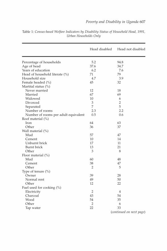
Table 1 presents a more detailed, census-based overview ofvariables associated with the head of household being disabled.Disability is thereby defined in accordance with the Ugandancensus manual, which defines disability as any condition whichprevents a person from living a normal social and working life.A head of household is considered disabled if this prevents him or
4 A direct question on the disability status of the respondents is not included.
606 J.G. Hoogevenn
Table 1: Census-based Welfare Indicators by Disability Status of Household Head, 1991,Urban Households Only
Head disabled Head not disabled
Percentage of households 5.2 94.8Age of head 37.6 34.7Years of education 6.2 7.6Head of household literate (%) 71 79Household size 4.7 3.9Female headed (%) 45 32Martital status (%)Never married 12 18Married 67 69Widowed 10 6Divorced 3 2Separated 7 5Number of rooms 2.3 2.2Number of rooms per adult equivalent 0.5 0.6
Type of tenure (%)Owner 39 28Normal rent 49 50Other 12 22
Fuel used for cooking (%)Electricity 2 4Charcoal 43 54Wood 54 35Other 2 6Tap water 22 33
(continued on next page)
Poverty and Disability in Uganda 607
her from being actively engaged in labour activities during the pastweek.5 Table 1 only comprises information for urban households(information on disability was only collected for a small fraction ofthe rural households) and does not report standard errors.The reason for the latter is that the information is based on the
Table 1 (continued)
Head disabled Head not disabled
Toilet facility (%)Flush 7 14Pit 82 76Other 12 11
Qualifications of head of household (%)None 81 71School certificate 9 13Professional certificate 6 8Diploma 2 3Degree 1 2Other 0 0
Education deficita
At age 12 1.1 0.9At age 18 2.2 1.9
Main source of livelihood of household (%)Subsistence farming 27 12Petty trade 25 15Formal trade 4 5Cottage industry 7 1Property income 2 2Employee income 21 45Other 14 19
Author’s calculations using the 1991 population census. The number of urbanhouseholds with a disabled head is 22165. The number of urban householdswithout a disabled head equals 425333.a Education deficit is defined as (age – 6) – number of years of education received.
5 The International Classification of Functioning (ICF; WHO, 2001) defines disabilityas the outcome of the interaction between a person with an impairment and theenvironmental and attitudinal barriers he/she may face. The ICF conceptualframework provides standardised concepts and terminology that can be used indisability measurement. Guidelines on how to measure disability have not beenagreed upon. Definitions therefore vary from study to study.
608 J.G. Hoogevenn
census, so there are no standard errors — at least none attributableto sample design. The descriptive statistics show that approxi-mately 5% of the households are headed by a disabled person andthat households headed by a person with disabilities are larger (4.7versus 3.9 members). Disabled heads are somewhat older (38 versus35), received less education (6.2 years as opposed to 7.6) and aremore likely to be illiterate (29 versus 21%) and female (45 versus32%). In terms of marital status there is little distinction betweendisabled and nondisabled heads, except for the fact that disabledheads are less likely to have never married (12 versus 18%) and aremore likely to be widowed (10 versus 6%). This may be a reflectionof disabled heads being older.
Turning to housing conditions, households headed by a disabledperson live in slightly larger houses (2.3 versus 2.2 rooms), thoughon a per capita basis housing space is smaller for householdsheaded by a disabled person. The quality of housing occupied byhouseholds with a disabled head is less. Though there is nodifference in the type of roofing material used, walls are morelikely to be made of low-quality materials like mud (57 versus47%) and unburnt brick (17 versus 11%) rather than of cement (10versus 14%) and burnt brick (13 versus 21%). Also, compared withnondisabled households, floors in disabled households are morelikely to be made of mud (60 versus 48%) and less likely to consistof cement (38 versus 47%). Households with a disabled head haveless access to tap water (22 versus 33%) and flush toilets (7 versus14%), and are more inclined to use wood as fuel for cooking (54versus 35%). Fifty-four per cent of the nondisabled households usecharcoal as the preferred fuel for cooking as opposed to 43% of thehouseholds with a disabled head. Remarkably, 39% of disabledhouseholds own their house, as opposed to 28% of the householdswith a nondisabled head. Putting together the various pieces ofinformation, it appears that disabled households live in lowerquality housing located in the urban outskirts where access tofirewood is easier, tap water is less readily available and it is easierto construct one’s own home.
That circumstances are worse in households headed by adisabled person is illustrated by housing conditions, but also bythe education deficit, which reflects the difference between thenumber of years a child should have been educated (according to itsage) and the actual years of education received. Children in
Poverty and Disability in Uganda 609
households headed by a disabled head receive less education. To theextent that education drives the ability to earn an income in thefuture, it confirms quantitatively the qualitative point made byLwanga-Ntale (2003) that the currently disabled are more likely topass their poverty on to their children.
Considering the main sources of income, disabled peopleparticipate less in the labour market than nondisabled people andare more likely to be self-employed. Whereas employee income isthe most frequently mentioned income source (45%) amongstnondisabled households, the most frequently mentioned sourcesof income for disabled households are subsistence farming (27%)and petty trade (25%). Amongst people with disabilities,employee income is only the third most important (21%) sourceof income.
3. Methodology
Whereas the information in Table 1 is informative about the non-consumption dimensions of poverty of households with adisabled head — and suggestive of poverty being higher, itdoes not provide actual information about the incidence ofconsumption poverty amongst disabled people. This sectionpresents a methodology to derive census-based consumptionpoverty estimates for people with disabilities. The methodologyused here was first described by Hentschel et al. (2000) and hasbeen refined by Elbers et al. (2002, 2003). Briefly, it comprisesregressing household survey per capita consumption on a set ofcontrol variables that are common to the survey and the census.Out of sample prediction on unit record census data is then usedto yield predicted per capita consumption for each household.Instead of calculating one prediction for each household, anumber of simulations (typically 100) are run in which thecoefficient vector is perturbed and errors are attributed to thepredicted per capita consumption. This yields (100) per capitaconsumption predictions for each household. By splitting thecensus data into households with and without a disabled headpoint estimates of various poverty indicators and their standarderrors can be calculated for each group.
Below a more in-depth overview of the method is presented. It isbased in part on Elbers et al. (2003) and Okiira Okwi et al. (2003).
610 J.G. Hoogevenn
3.1 Deriving Welfare Estimators for Small Target Populations
For a household h in location c the (natural logarithm of) householdper capita consumption, ln ych, can be written as the expected valueof per capita consumption conditional on a set of householdcharacteristics, Xch, that are common to both the survey and thecensus, and an error term nch. Xch does not comprise householdspecific information on disability as this is unavailable in the samplesurvey.6
Ln ych ¼ E�Ln ychjXch
�þ vch: ð1Þ
If there are more households within one location — as is commonfor household surveys and applicable to the survey used in thispaper — the error term can be thought to consist of a locationcomponent, hc, and an idiosyncratic household component, 1ch, andcan be written as: nch ¼ hc þ 1ch. Using a linear approximation to theconditional expectation in (1), the household’s logarithmic percapita expenditure can then be modelled as:
Ln ych ¼ XTchbþ hc þ 1ch; ð2Þ
which is estimated using Generalised Least Squares, thus allowingfor heteroskedasticity in 1ch.
7,8 In order to do so, a logistic model isestimated of the variance of 1ch with a set of variables zch asregressors, comprising ych, Xch, their squares and all potentialinteractions.
The log of the variance is rewritten such that its predictionis bound between 0 and a maximum A, set equal to 1.05 £ max(12ch):
6 Xchmay, however, comprise disability information obtainable from the censusthat can be included in the survey, such as the fraction of disabled households inthe enumeration area or its interactions with household characteristics.
7 To allow maximum flexibility different models are estimated for each stratum ofthe national household survey. For this paper four models were estimated, forrespectively the Central, Eastern, Northern andWestern regions. Table 6 presents,for illustrative purposes, the model derived for the Northern region. Theregression models are not very informative by themselves as they only comprisethose welfare correlates that work ‘best“ in explaining per capita consumptionand do not have a causal interpretation.
8 In theory it is possible to also allow for heterogeneity in hc. In practice the numberof observations is too small to do so (namely the number of clusters in thestratum).
Poverty and Disability in Uganda 611
Ln12ch
A 2 12ch
!¼ zT
chaþ rch: ð3Þ
Estimation of (2) and (3) yields the coefficient vectors a and b. Incombination with household characteristics Xch from the census aprediction of the log consumption for each household in the census,ln yh, can be made. The accuracy of this predicted per capitaconsumptiondepends on the properties of the regressionmodel, andespecially on the precision of the model’s coefficients and itsexplanatory power. As the interest is in the welfare estimates andtheir standarderror, anumberof predictions is generatedbydrawinga set of ~b coefficients along with location and idiosyncraticdisturbances. The ~b coefficients are drawn from the multivariatenormal distributions described by their respective point estimates, b,and the associated variance covariance matrix. The idiosyncraticerror term, ~1ch, is drawn from a household-specific normal9
distribution with variance ~s 21;ch which is derived by combining the
a coefficients with the census data.10 The location error term, ~hc, isdrawn from a normal distribution with variance ~s 2
h , which itself isdrawn fromagammadistributiondefined so as to havemean s 2
h andvarianceVðs 2
h Þ. Thedrawn coefficients ~b, ~hc and ~1ch are used to arriveat the simulated predicted per capita expenditure:
Ln ~ych ¼ XTch~bþ ~hc þ ~1ch: ð4Þ
By repeating this process — typically 100 times — a full set ofsimulated household per capita expenditures is derived.
Welfare estimates are based on individuals rather than onhouseholds, and this has to be accounted for. If household h hasmh family members, then the welfare measure can be written asW(m, yh, u), where m is the vector of household sizes, yh ishousehold per capita expenditure and u is a vector of disturbances.Disturbances for households in the target population are unknownby definition and cannot be determined. What can be determined is
9 Emwanu, Okiira Okwi and Hoogeveen, who derived the initial set of census-based poverty estimates for Uganda experimented with various t and non-parametric distributions, and found that the results are robust to the choice ofdistribution.
10 Letting exp zTcha
� �¼ B and using the delta method, the model implies a
household specific variance estimator of s21;ch ¼ AB
1þB
� �þ 1
2 VarðrÞ ABð12BÞð1þBÞ3
� �.
612 J.G. Hoogevenn
the expected value of the welfare indicators given household sizeand the census-based predicted household per capita expenditure.After defining an indicator variable, d, taking the value 1 if the headof household is disabled and 0 otherwise, the expected value of thewelfare indicator can be denoted as:
~md ¼ E½Wdjm; ~yh; d�: ð5Þ
Based on (5), welfare measures (and their standard errors) can becalculated for households with and without a disabled head. Thevariable d may take more than two distinct values and could alsoreflect the location of the household. This is the more conventionalapproach in small area welfare estimation, yet the possibilities fordisaggregation are not limited to disability status or location.Estimates may be disaggregated by any household characteristicobtainable from the census, including household size, educationalattainment, age of head of household, occupation, ethnic back-ground or gender, making it possible to generate highly disag-gregated census-based poverty profiles.
The performance of these census-based welfare estimators may bejudged by their ability to replicate the sample survey’s welfareestimates (at the lowest level of representative disaggregationattainable) and the size of the standard error of the census-basedwelfare estimators for smaller target populations.Theprediction errordepends mostly on the accuracy with which the model’s coefficientshave been estimated (model error) and the explanatory power of theexpendituremodel (idiosyncratic error).11 Determined by the proper-ties of the expenditure model and the sensitivity of the welfareestimator to deviations in expenditure, the variance attributable tomodel error is independent of the size of the target population. Thevariance due to idiosyncratic error falls approximately proportion-ately in thenumberofhouseholds in the targetpopulation(Elbers et al.,2003). That is, the smaller the target population, the greater is thiscomponent of the prediction error. This puts a limit to the degree ofdisaggregation feasible. There is also a limit towhich aggregationwillincrease precision.As location is related to household consumption, itis plausible that some of the effect of location remains unexplainedeven with a rich set of household specific regressors. The greater11 Simulation introduces another source of error in the process: computational
error. Its magnitude depends on the method of computation and the number ofrepetitions. With sufficient resources it can be made as small as desired.
Poverty and Disability in Uganda 613
the fraction of the total disturbance that canbe attributed to a commonlocationcomponent the lessonebenefits inprecision fromaggregatingover more households.
4. Data
Two data sets are used to arrive at small area welfare estimates forUganda: unit record data from the population census andinformation from the Integrated Household Survey (IHS). ThePopulation and Housing Census was administered in January 1991,covering 450,000 urban households and 3.0 million rural house-holds. It comprised, for all household members, information onhousehold composition, ethnic background, marital status andeducational attainment. For urban households a ‘long’ form wasadministered which collected additional information on activitystatus, housing conditions, types of fuel used and sources of water.Based on the responses given on the previous week’s activity status,it determined whether a head of household was disabled.
The IHS was administered between January and December 1992,and is of the World Bank’s Living Standards Measurement Studytype. It is representative at the regional level (Central, East, Northand West) for urban and rural areas, and has been used as basis forUganda’s official poverty lines and statistics (Appleton, 2001).
Table 2 presents poverty estimates based on these sources ofinformation. It shows the Foster–Greer–Torbecke measures(FGT(a)), with a-values of 0, 1 and 2 reflecting respectively povertyincidence, the poverty gap and its square. Three sets of povertyestimates are presented: the official poverty statistics derived fromthe IHS alone, census-based estimates derived after combiningcensus and survey data (taken from Okiira Okwi et al., 2003), and aset of estimates generated after interacting the original census-basedmodel with the fraction of disabled households in each enumerationarea. The latter estimates are preferred because they exploitthe available disability information from the census.12 The tableshows that the point estimates are not identical, but a t-test does notreject the equality of IHS and census-based poverty estimates at
12 There may be interest in the poverty estimates derived from the original censusmodel. These are presented in Table A1. The predictions from both models arehighly comparable, the main difference being that the standard errors on thedisability model are somewhat larger.
Standard errors are in parentheses. The IHS and census-based estimates are from Okiira Okwi et al. (2003). The estimates forthe disability model are derived after interacting all variables of the census-based model with the fraction of disabledhouseholds in the primary sampling unit, and maintaining those interacted variables in the model that were significant at the95% confidence level while keeping all variables from the census-based model. The poverty lines are from Appleton (2001).They are expressed in 1989 shillings.
Pov
ertyan
dD
isabilityin
Ug
and
a615
the 95% level of significance. In other words, once it is taken intoaccount that poverty estimates are associated with a standard error,it is not possible to distinguish the survey- and census-basedpoverty estimates. In the remainder of the paper the census-basedpredictions of the disability model are used to obtain povertyestimates for disabled and nondisabled households.
5. Poverty amongst People with Disabilities
Section 3 has shown that reporting consumption poverty for a lesspopulous vulnerable group such as people with disabilities shouldbe feasible if disability is recorded in the census. Such povertyestimates for those who live in a household with a disabled head arepresented below. It is believed that assessing the poverty status ofhouseholds with a disabled head is most revealing as the head ofhousehold is typically one of the main breadwinners. Note thatestimates on intra-household differences in poverty betweendisabled and nondisabled household members are not presented.As the welfare estimates are based on per capita householdconsumption, it is not possible to report such differences. Nor areestimates presented on poverty amongst those who live in house-holds where a person other than the head of household isdisabled.13
Table 3 presents the number of people living in households withand without a disabled head along with mean per capitaconsumption and various poverty measures. On average, 5% ofthe urbanites live in a household with a disabled head, but thisfigure hides substantial regional variation. The largest percentage ofindividuals living in a household with disabled head is found inNorthern Uganda, 14%. The smallest percentage, 3%, is reported forCentral Uganda, the most urbanised region of the country andhome to Kampala, Uganda’s capital city.
With respect to poverty, the percentage of urban dwellers whostay in a household with a disabled head and who live in poverty isconsiderably larger than that for those who stay with a nondisabled
13 This suggests another application: identifying the welfare consequences of thepresence of disabled dependents in the household. Households in which adisabled person is present may, ceteris paribus, earn less income becausedisabled people are likely to earn less, or because others need to forego incometo care for the disabled person.
616 J.G. Hoogevenn
Table 3: Welfare of Urban Dwellers Living in Households With and Without a Disabled Head, 1992 (Disability Model)
Author’s calculations. Standard errors in parentheses. Per capita consumption is expressed in 1989 shillings. The povertyestimates are based on the disability model. Estimates derived from the ‘official’ poverty mapping model are very comparable— e.g., national poverty rates are 42 and 25% for disabled and nondisabled households, respectively, are associated withsomewhat smaller standard errors. These estimates are included in Table A1.
Pov
ertyan
dD
isabilityin
Ug
and
a617
head: 43% as opposed to 27%. In other words, the (populationweighted) probability that people who stay in a household with adisabled head live in poverty is 60% higher14 than that of peoplewho stay in a household with a nondisabled head. There isconsiderable regional variation in poverty. This holds for disabledand nondisabled households. Amongst those living in householdswith a disabled head, the level of poverty is highest in the Northernregion, at 59% (compared with 51% for nondisabled), and lowest inthe Central region, 28% (compared with 19% for nondisabled). Notonly is the incidence of poverty worse amongst households withdisabled heads, the severity of poverty, as measured by the povertygap and the poverty gap squared, is greater amongst householdsheaded by disabled persons. This holds across all regions.
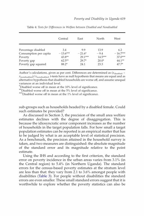
Table 4 considers the differences in poverty between householdswith and without disabled heads in more detail. It presents thepercentage difference between the two groups and shows t-testresults on the equality of the various poverty indicators.
The results illustrate the plight of people with disabilities. Interms of per capita consumption, consumption amongst householdswith disabled heads is 14–22% lower than in households withnondisabled heads, depending on the region. Poverty incidence is15–44% higher in households with disabled heads. And the resultsfor the poverty gap and poverty gap squared show that the depth ofpoverty is higher amongst disabled people as well. So, not only arehouseholds with disabled heads more likely to be poor, but thedegree of poverty is greater as well.
The t-tests reported in Table 4 show that the differences inpoverty between disabled and nondisabled people are highlysignificant. In none of the regions is the hypothesis that disabledand nondisabled people have identical means accepted at signifi-cance levels of 5% or less; the same holds for almost all otherindicators.
6. How Much Can We Disaggregate?
There is likely to be interest in disability statistics at levels ofdisaggregation below the region, for instance for each district, or for
14 Calculated as (42.8–26.7)/26.7.
618 J.G. Hoogevenn
sub-groups such as households headed by a disabled female. Couldsuch estimates be provided?
As discussed in Section 3, the precision of the small area welfareestimates declines with the degree of disaggregation. This isbecause the idiosyncratic error component increases as the numberof households in the target population falls. For how small a targetpopulation estimates can be reported is an empirical matter that hasto be judged by what is an acceptable level of statistical precision.As a benchmark, the precision attained in the household survey istaken, and two measures are distinguished: the absolute magnitudeof the standard error and its magnitude relative to the pointestimate.
Using the IHS and according to the first criterion, the standarderror on poverty incidence in the urban areas varies from 3.1% (inthe Central region) to 5.4% (in Northern Uganda). The standarderrors for the census-based poverty estimates at the stratum levelare less than that: they vary from 2.1 to 3.6% amongst people withdisabilities (Table 3). For people without disabilities the standarderrors are even smaller. These small standard errors suggest that it isworthwhile to explore whether the poverty statistics can also be
Table 4: Tests for Differences in Welfare between Disabled and Nondisabled
Central East North West
Percentage disabled 3.4 9.9 13.9 6.2Consumption per capita 213.6*** 221.6* 29.4 216.7***Poverty 43.8** 29.1*** 14.5*** 37.0***Poverty gap 62.5** 29.7* 20.0* 44.1**Poverty gap squared 88.2* 24.1 23.3 47.7*
Author’s calculations, given as per cent. Differences are determined as (xdisabled –xnondisabled)/xnondisabled. t-tests have as null hypothesis that means are equal and asalternative hypothesis that disabled households are worse off, and assume unequalvariances at an individual level.*Disabled worse off in mean at the 10% level of significance.**Disabled worse off in mean at the 5% level of significance.***Disabled worse off in mean at the 1% level of significance.
Poverty and Disability in Uganda 619
reported at lower levels of aggregation, for instance at the districtlevel. Comparing district level standard errors obtained for house-holds with disabled heads with the highest standard error from thehousehold survey (5.6%), this threshold is exceeded in 17 of the 38districts. For households without disabled heads the results aremore encouraging. Only in two districts do the standard errorsexceed the threshold of 5.6%.
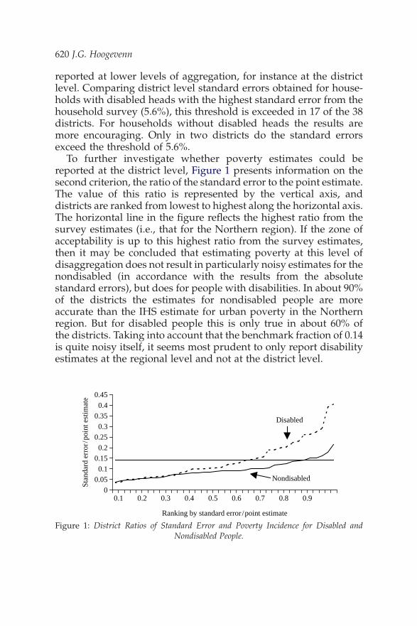
To further investigate whether poverty estimates could bereported at the district level, Figure 1 presents information on thesecond criterion, the ratio of the standard error to the point estimate.The value of this ratio is represented by the vertical axis, anddistricts are ranked from lowest to highest along the horizontal axis.The horizontal line in the figure reflects the highest ratio from thesurvey estimates (i.e., that for the Northern region). If the zone ofacceptability is up to this highest ratio from the survey estimates,then it may be concluded that estimating poverty at this level ofdisaggregation does not result in particularly noisy estimates for thenondisabled (in accordance with the results from the absolutestandard errors), but does for people with disabilities. In about 90%of the districts the estimates for nondisabled people are moreaccurate than the IHS estimate for urban poverty in the Northernregion. But for disabled people this is only true in about 60% ofthe districts. Taking into account that the benchmark fraction of 0.14is quite noisy itself, it seems most prudent to only report disabilityestimates at the regional level and not at the district level.
0
0.050.1
0.150.2
0.250.3
0.350.4
0.45
0.1 0.2 0.3 0.4 0.5 0.6 0.7 0.8 0.9
Ranking by standard error /point estimate
Stan
dard
err
or/p
oint
est
imat
e
Disabled
Nondisabled
Figure 1: District Ratios of Standard Error and Poverty Incidence for Disabled andNondisabled People.
620 J.G. Hoogevenn
One reason for the observed increase in standard errors is that insome districts the number of urban households is small — and thenumber of households with a disabled head is even smaller.Disaggregation into categories that avoid having small numbers insome of the cells is possibly a better approach. For instance, about31% of the people live in female-headed households. Table 5 showsthat such a breakdown by disability status of head of household isindeed feasible, in that the maximum standard error obtained, 4.3%,is considerably less than the highest standard error for the IHS of5.4%. Yet, few of the differences are significant at the 95% level ofsignificance. This, however, is less a result of the somewhat largerstandard errors and more the consequence of the relatively smalldifferences in poverty incidence between male- and female-headedhouseholds.
7. Is Poverty amongst People with Disabilities Estimatedwith Bias?
Consider again the expenditure model presented in Section 3 that isestimated using the survey data:
Table 5: Poverty by Gender and Disability Status of Head of Household, Urban Households1992.
Nondisabled Disabled
Male Female Male Female
Central 17.9 22.6 25.9 30.9(1.6) (2.0) (3.6) (3.9)
East 36.7 39.2 47.6 49.5(1.9) (2.0) (2.8) (2.7)
North 52.1 48.9 59.8 56.8(2.2) (2.4) (2.3) (2.2)
West 32.4 37.7 43.5 51.9(1.7) (2.6) (3.5) (4.3)
Author’s calculations. Standard errors in parentheses.
Poverty and Disability in Uganda 621
Ln ych ¼ XTchbþ hc þ 1ch: ð2Þ
If the sample survey does not collect information on disability, thenthe welfare correlates of model (2), the X-variables, only capture alimited impact of disability, namely that captured by the census-derived means on the fraction of disabled households in anenumeration area (ea) and the interactions of these ea-means withhousehold specific variables.
To the extent that the consequences of disability are captured bythe fact that people with disabilities live in houses of lower quality,have lower educational attainment, have less access to tap water,use different sources of fuel and are less likely to work as a paidemployee — as Table 1 indicates (i.e., the X-variables for peoplewith disabilities differ from those without disabilities) — the modelcaptures their welfare status correctly. The same is true if theconsequences of disability are the result of community effects.However, people with disabilities may also differ from thosewithout disabilities in that their bs are different. Stigmatisation andlow self-esteem are characteristics of people with disabilities(Yeo and Moore, 2003) that are likely to have systematicconsequences for consumption levels. For given levels of education,discrimination in the labour market or physical constraints arelikely to lead to returns to education that are different for peoplewith disabilities.
Suppose that one could estimate instead of model (2), anextended model (2*) which includes interaction terms of X withan indicator variable d taking the value one if the head of householdis disabled and which is zero otherwise:
In ych ¼ XTchbþ ðdXÞTchgþ hc þ 1ch: ð2pÞ
If (2*) is the correct model and the gs are significantly different fromzero, then estimating (2) leads to the inclusion of omitted (disability)information in the error term. If, when predicting householdconsumption from the census, this differential effect is ignored (i.e.,the gs are assumed to be zero), predicted consumption will bebiased. Which way the bias goes depends on the sign of the gs. If thegs are negative, predicted consumption is too high and poverty isunderestimated. If the gs are positive, predicted consumption is toolow and poverty is overestimated.
622 J.G. Hoogevenn
For many small target populations the direction of the bias ishard to determine a priori. But in the case of disability it is plausiblethat the gs are negative, and zero at best. Stigmatisation and lowself-esteem are likely to have negative consequences for consump-tion. Discrimination in the labour market and physical constraintswill contribute to a lower correlation of education with consump-tion. If the assumption that the gs are negative iscorrect, consumption amongst people with disabilities is over-estimated, and the poverty figures presented in Section 5 are aconservative estimate of the true poverty amongst people withdisabilities.15
Most variables used in the models to predict consumption,however, are correlates of household consumption — type of roof,access to clean water, the type of fuel used— for which there is littlereason to assume that their association to consumption is differentfor disabled and nondisabled people. Only some of the variables inthe models are determinants of consumption that may be prone tobias.16 This can be illustrated with the model for Northern Ugandapresented in Table 6. Of the 32 variables, most reflect householdcomposition, the type of housing, the degree to which childrenmissed out on their education or a combination of these. Five of the32 variables reflect the level of education of different members of thehouseholds. Their coefficients could have a more structuralinterpretation, and could be prone to bias.
Further light on the presence of bias is shed by the six variablesthat reflect interactions between the fraction of disabled people inan enumeration area and other household characteristics. If therewould be bias such that the structural variables of the model donot correctly reflect the bs for disabled people, one expects thatthe set of variables that presents interactions between the fractionof disabled in a community and other household characteristicswould correct for it. One thus expects structural variables toappear prominently amongst these interaction terms. Yet out of
15 This is reinforced by the fact that who becomes head of household isendogenous. As disability has greater deleterious effects on individualincome, it becomes less likely that the individual is in a position to head theirown household, possibly leading to the exclusion of the more severely disabledpeople from the analysis.
16 The reason for allowing endogenous variables in the model is that the objectiveis to obtain a set of variables that can give a precise estimate of the expectedvalue of per capita consumption (see also equation 1).
Poverty and Disability in Uganda 623
Table 6: Regression Model for Northern Uganda.
Variable Coefficient t-statistic
Intercept 10.918 81.4Number of males withsecondary education
0.115 3.6
Maximum number of yearsof education in household
0.022 3.9
Maximum education deficit forthose aged 13
0.023 3.4
Log of household size 20.846 217.8Household size is 5 0.157 2.5Fraction of males aged50 and over squared
20.375 23.6
Number of females aged 25 or less 0.086 5.1Roof is not madeof thatch, asbestos, cement or tiles
20.190 23.3
Floor is made of mud 20.281 24.4Household owns the house 0.239 4.8Tenure is free of charge 20.188 23.5Cooking on charcoal or wood 20.295 26.3Interactions of household variablesand enumeration area means(from census)/district dummiesHead of household married,separated or divorced £ Iron roof (ea)
0.428 3.2
Female headed household £ Districtdummy for Nebbi (d)
0.260 2.4
Maximum number of yearsof education £ Lives in house withsubsidised rent (ea)
20.039 22.4
Mean education deficit atage 13 £ Walls made of mud (ea)
20.085 22.8
Maximum number of yearsof education £ District dummy for Kitgum (d)
20.029 24.9
Maximum number of yearsof education £ District dummy for Nebbi (d)
0.036 3.2
Household size is 9 (ea) 6.483 5.0Proportion of females aged 6 2 14 (ea) 23.386 22.8
(Continued on next page)
624 J.G. Hoogevenn
the 19 interaction terms included in the model of Table 6, only sixcomprise interactions with the fraction of disabled people in acommunity. Out of these six, only one includes a structuralvariable, namely the number of males with secondary
Table 6 (continued)
Variable Coefficient t-statistic
Number of males aged30 and over £ Number of Gisu perhousehold (ea)
23.840 22.6
Number of males aged30 and over £ District dummy for Lira (d)
20.174 22.8
Number of males aged 30and over £ District dummy for Moroto (d)
0.429 3.9
Iron roof £ Main source of livelihoodis in formal trade (ea)
0.721 2.6
Household has no toilet£ District dummy for Gulu (d)
0.488 3.2
Interactions with fraction ofdisabled heads of householdin census enumeration areaMean education deficit atage 13 £ Number of Gisu perhousehold (ea) £ Fraction of disabled (ea)
16.222 3.5
No. of males withsecondary education £ Hh uses electricity forcooking (ea) £ Fraction of disabled (ea)
2262.05 22.4
Proportion of females aged30 2 49 squared £ Fraction of disabled (ea)
1.862 4.2
Log adult equivalent householdsize £ District dummy for Moyo (d)£ Fraction of disabled (ea)
20.345 22.5
Number of males aged30 and over £ Hh uses electricity forcooking (ea) £ Fraction of disabled (ea)
773.195 4.0
Household has no toilet£ Lives in house withsubsidised rent £ Fraction of disabled (ea)
232.565 23.8
The dependent variable is log per capita consumption. (ea) indicates a mean takenfor the enumeration area calculated from unit record census data. (d) indicates adistrict variable. The total number of observations is 658. The adjusted R2 is 0.64.
Poverty and Disability in Uganda 625
education,17 and this only in interaction with use of electricity asa source of fuel. The latter is used by only 2% of the population(Table 1). So, when predicting household consumption, thisinteraction term is relevant for only a very small fraction of thepopulation. This seems to suggests that underestimation ofconsumption for disabled people due to different bs for structuralvariables is a limited problem.
A conceptual paper by Van der Weide (2005) suggests ways tofurther explore whether any of the coefficients are biased. The paperasks what would be the consequences if only one model wereestimated and consumption predicted from it, while in fact twomodels of reality exist (say, one for nondisabled and one fordisabled people). It could be that the model that is estimatedprovides a reasonable description for one section of the populationbut that a different model applies to the other section of thepopulation. On average, such differences may not be notable,especially when one of the groups is small. If this model is then usedto obtain consumption predictions for, say, administrative units, theestimates may be quite reasonable (i.e., the model’s predictions ofpoverty and the survey’s prediction would be similar — as is thecase in Table 2) and the structural error in the model may gounnoticed. Yet, once disaggregated by group — as is done in thispaper — group-based predictions for consumption will be biased.
There are at least two avenues to investigate the presence of suchstructural error. A first approach does so by estimating a model forenumeration areas rather than for households. In doing so it finds alevel of aggregation at which both consumption information (fromthe survey) and information about disability (from the census) areavailable. Hence one could estimate:
In �ych ¼ �XTchbn þ ndc
�XTdcðbd 2 bnÞ þ nch ð6Þ
where ndc measures the fraction of disabled households, d, inenumeration area c, where an upper bar denotes means and wherench denotes a zero expectation error term that is uncorrelated withthe explanatory variables. Equation (6) could then be estimated by
17 Another interaction term comprises the education deficit at age 13. Yet this is aconsumption correlate, as young children cannot be expected to substantiallycontribute to household income.
626 J.G. Hoogevenn
obtaining �ych from the survey and the right hand side variables fromthe census.18
Another approach uses an auxiliary model to estimate, in thecensus, the probability of being disabled. It then takes the predictedprobabilities to the survey and estimates:
In ych ¼
XTa;ch bn þ ha;ch with probability ð12 pdÞ
XTd;ch bd þ hd;ch with probabilitypd
8<: ð7Þ
where hch is a zero expectation error term, pd reflects the probabilityof being disabled and underscore a refers to nondisabled people.This model could be estimated in a two step procedure. In the firstthe auxiliary model is estimated (say a logit or probit) from data inthe census only. In the second step, the coefficients from theauxiliary model are used to derive estimates of the probability pd inthe survey and to formulate a likelihood function that only has theconsumption coefficients as unknown parameters.
The first approach uses information that is readily obtainablefrom the census and the survey. Whether it can be estimatedaccurately depends on the loss in information from estimating amodel for enumeration areas. In a typical household survey, about10–20 households are selected from each enumeration area, so thisapproach leads to a considerable reduction in information. But ifthere is sufficient variation across the enumeration areas one mightbe able to estimate equation (6), especially since in a two-typeapproach there is less need to estimate stratum specificmodels (as isthe case for poverty mapping) so that one gains observations byonly estimating one model for the nation as a whole. The success ofthe second approach depends on the accuracy with which thediscrete choice model can predict the probability of being disabled.
For both approaches hold that, apart from estimating correctmodels, which in and by itself is informative about the accuracy ofthe estimates, there exist unresolved issues on how to get toconsumption predictions. To date, both approaches have beendescribed but not tested empirically. Doing so would not onlypermit an assessment of the assertion made here — that povertyamongst disabled can be accurately measured using existing
18 A more efficient way to estimate (6) is to estimate:
In ych ¼ XTchbn þ ndc
�XTdcðbd 2 bnÞ þ y ch.
Poverty and Disability in Uganda 627
poverty mapping models — it would also allow the focus to beexpanded beyond disabled people.19
8. Conclusion
Reliable statistics relating to consumption poverty amongstvulnerable groups can potentially go a long way to motivate policymakers to take action. To date, such data have been lacking. Onereason for this is that vulnerable groups are typically numericallysmall. Being less populous, only a limited number of householdsfrom the population group of interest are captured in householdsurveys. And with few observations, accurate poverty numberscannot be generated, leading to the statistical invisibility of smallvulnerable groups.
By combining census with survey data, estimates of consumptionpoverty can be derived for less populous groups. Provided thatinformation that identifies the small vulnerable group is recorded inthe census, it is possible to generate these estimates. Hence povertystatistics for people with disabilities, orphans, child-headed house-holds or ethnic minorities can be generated.
In this paper, the focus is on poverty in households with adisabled head. It has been shown that the numbers support thequalitative evidence on poverty amongst disabled people. In urbanareas consumption poverty amongst households with a disabledhead is 43%, as opposed to 27% for households with a nondisabledhead. The (population weighted) likelihood that people who stay ina household with a disabled head live in poverty is 60% higherthan that of people who stay in a household with a nondisabledhead.
The estimates presented in this paper are preliminary andmay bebiased. Depending on the characteristics of the group of interest, thepredications may over- or underestimate consumption poverty.An underestimation of poverty occurs if the group of interest hascharacteristics (unobserved in the survey) that induce it to havelower consumption; poverty will be overestimated if the reverse isthe case. A first analysis of whether there is bias suggests that thebias is likely to be small and, if present, is likely to lead to anunderestimation of poverty amongst disabled people.19 Work in this area is progressing as part a research program funded by the Bank
Netherlands Partnership Program.
628 J.G. Hoogevenn
The estimates are based on information from the 1991 UgandanPopulation and Housing Census and the 1992 IHS, and thepoverty estimates pertain to this period. This makes theinformation somewhat dated, especially in view of the largetransitions that the Ugandan economy has experienced recently.This is illustrated by the remarkable decline in poverty in the1990s, from 56% in 1992 to 34% in 1999, and the rise thereafter to38% in 2002. Such profound changes are likely to haveconsequences for poverty amongst people with disabilities. In2002 a new census was implemented, and it is expected that in thenear future census-based welfare estimates will become available.These can then be used to create a more up-to-date profile ofpoverty amongst people with disabilities and to gain experiencewith the two alternative methods that, if the models can beestimated precisely, would provide unbiased estimates of povertyamongst disabled people.
References
Appleton, S. (2001) ‘Changes in Poverty and Inequality 2001’, inR. Reinikka and P. Collier (eds), Uganda’s Recovery: The Role ofFarms, Firms and Government, Washington DC: World Bank, Ch. 4.
Elbers, C., J.O. Lanjouw and P. Lanjouw (2002) ‘Welfare in Villagesand Towns: Micro Level Estimation of Poverty and Inequality’,Policy Research Working Paper No. 2911, Washington DC: WorldBank.
Elbers, C., J.O. Lanjouw and P. Lanjouw (2003) ‘Micro LevelEstimation of Poverty and Inequality’, Econometrica, 71: 355–64.
Ghosh, M. and J.N.K. Rao (1994) ‘Small Area Estimation: AnAppraisal’, Statistical Science, 9: 55–93.
Hentschel, J., J.O. Lanjouw, P. Lanjouw and J. Poggi (2000)‘Combining Census and Survey Data to Trace the SpatialDimensions of Poverty: A Case Study of Ecuador’, World BankEconomic Review, 14: 147–65.
Hoogeveen J., E. Tesliuc, R. Vakis and S. Dercon (2004) ‘A Guide tothe Analysis of Risk, Vulnerability and Vulnerable Groups’,available at http://wbwebapps5/wwwextweb/sp/risk_management/PDF_files/RVA-V6.pdf.
Lwanga-Ntale, C (2003) ‘Chronic Poverty and Disability inUganda’, unpublished manuscript.
Metts, R. (2000) ‘Disability Issues, Trends and Recommendations forthe World Bank’, Social Protection Discussion Paper No. 7,Washington DC: World Bank.
Okidi, J.A. and G.K. Mugambe (2002) ‘An Overview of ChronicPoverty and Development Policy in Uganda’, Working Paper No.11, Chronic Poverty Research Centre.
Okiira Okwi, P., T. Emwanu and J.G. Hoogeveen (2003) ‘Poverty andInequality in Uganda: Evidence from Small Area EstimationTechniques’, unpublished manuscript.
Republic of Uganda (2002) Second Participatory Poverty AssessmentProcess: Deepening the Understanding of Poverty, Kampala: Ministryof Finance, Planning and Economic Development.
Van der Weide, R. (2005) ‘Accurate Assessment of Poverty Amongthe Disabled’, unpublished manuscript.
WHO (2001) International Classification of Functioning Disability andHealth — ICF, Geneva: World Health Organisation.
Yeo, R. and K. Moore (2003) ‘Including Disabled People in PovertyReduction Work: “Nothing About Us, Without Us”’, WorldDevelopment, 31: 571–90.
Appendix
Table A1
630 J.G. Hoogevenn
Table A1: Welfare of Urban Dwellers Living in Households with and without a Disabled head, 1992 (Census Model)