Mechanical characterization of soft materials: … · Adequate mechanical characterization of soft...

Report Number

ETH/ZfM-2008/01

February 2008

Institute of Mechanical Systems Department of Mechanical and Process Engineering ETH Zurich

Marc Hollenstein

Mechanical Characterization of Soft Materials: Comparison between Different Experiments on Synthetic Specimens

February 24, 2005

Mechanical Characterization of soft Materials:Comparison between different Experiments on synthetic Specimens

Marc Hollenstein

Supervisors: Davide Valtorta, Alessandro Nava

Report on Diploma Thesis prepared for Prof. Dr. E. Mazza, Center of Mechanics, ETH Zurich

1 of 121

Table of Contents

Table of Contents

Table of Contents 2

Nomenclature 3

Abbreviations 6

1.0 Introduction - The Task, its Background and the Procedure 71.1 Background and Motivation: ‘Characterization of soft Materials’ 71.2 Task and Procedure 8

2.0 Measurement Methods: Devices and Experiments 92.1 Aspiration Experiment [20] 92.2 Torsional Resonator Device (TRD) and Experiment [18] 112.3 TeMPeST Test [22] 162.4 Large-scale spherical Indentation Tests 192.5 Classical Methods 20

3.0 Materials 233.1 Silicone Rubber 233.2 Liver 24

4.0 Theory, Derivations and Concepts 264.1 Theory of finite Elasticity [17] 264.2 Analytical Investigation of the Rheological Torsion Test 394.3 Analytical Determination of Eigenfrequencies of the TC2 514.4 Error-Factor for the ‘quasi-dynamic’ TeMPeST-Formula 554.5 Novel numerical Determination of Kappa Correction Factor 624.6 Investigation on elastic Material Response to finite Indentation 66

5.0 Results - Analysis and Discussion 735.1 Classical Methods 735.2 TRD-Experiment 775.3 Aspiration Experiment 805.4 TeMPeST Test 835.5 Large-scale spherical Indentation Test 104

6.0 Resume of Achievements and Conclusions 1136.1 Comprehensive mechanical Characterization of TC2 Silicone 1136.2 Investigated Limits of the TeMPeST Test 1146.3 Large-scale Indentation Test 1156.4 Final Remark and Acknowledgments 115

References 116Books, Literature 116Papers 117

List of Figures 119

List of Tables 121

2 of 121

Nomenclature

Nomenclature

Roman Alphabet

A cross-sectional area

B left Green deformation tensor

C right Green deformation tensor

Cno hyperelastic material parameters (5th order reduced polynomial form)

cp, cp* primary wave speed and complex correspondent

cs, cs* secondary wave speed and complex correspondent

D hyperelastic material parameters (5th order reduced polynomial form)

d diameter

Ee, Ee* initial (engineering) Young’s modulus and complex correspondent

E Lagrangian strain tensor

E extension

Eequi equivalent strain

e dilatation (unit volume change)

F deformation gradient

f frequency

FWVC fractional volume in compression

FWVT fractional volume in tension

Ge, Ge* initial (engineering) shear modulus and complex correspondent

G1, G2 real and imaginary component of complex shear modulus Ge*

h thickness of stratum

I identity matrix

Ip polar geometrical moment of inertia

I1, I2, I3 strain invariants

reduced strain invariants

i basic imaginary unit

k, k* wave number and complex correspondent

N axial (normal) force

P indentation force

p hydrostatic pressure stress

R0 cylinder radius

r0 radius of rigid right circular indenter

ri relative indentation

S second Piola-Kirchhoff stress tensor

T Cauchy stress tensor

T torque

t time

U strain-energy potential

I1 I2 J, ,

3 of 121

Nomenclature

Greek Alphabet

Mathematics

u displacement vector

V volume

VC volume in compression

VT volume in tension

Wp polar section modulus

u, v, w Cartesian components of displacement vector u

cylindrical components of displacement vector u

x, y, z Cartesian coordinates in present (deformed) configuration

X, Y, Z Cartesian coordinates in reference configuration

cylindrical coordinates in present (deformed) configuration

cylindrical coordinates in reference configuration

phase shift between excitation and system response

shear strain

Kronecker delta

indentation depth

engineering strain

bulk modulus, radius of gyration, kappa correction factor

torsion angle

stretch

wave length and complex correspondent

hyperelastic material parameter (neo-Hookean form), coefficient of friction

Lamé constant of elasticity

Poisson’s ratio

mass density

engineering stress

shear stress

phase of modulus

angular frequency

,i derivative with respect to i

transpose of matrix A

derivative of a with respect to time

absolute value of a

ur uθ uz, ,

r θ z, ,

R Θ Z, ,

α

γ

δi j

δz

ε

κ

ϑ

λ

λ λ∗,

µ

µe

ν

ρ

σ

τ

ϕ

ω

A′

a·

a

4 of 121

convolution product

vector (cross) product

scalar product

Re(_) real part of brackets

Im(_) imaginary part of brackets

⊗

×

•

5 of 121

Abbreviations

Abbreviations

CT computed tomography

TC2 TruthCube2

FEM finite element method

TeMPeST Tissue Property Sampling Tool

TRD Torsional Resonator Device

6 of 121

Introduction - The Task, its Background and the Procedure

1.0 Introduction - The Task, its Background and the Procedure

This report has been written in the frame of the diploma thesis elaborated at the ‘Center of Mechanics’ in the ninth semester of study at the ‘Mechanical Engineering Department’ of ETH Zurich.

The report features a complete description of the task, its background and the working procedure - analysis methods, theory and respective deriva-tions - together with discussions of the results and final conclusions.

A first part introduces the different measurement devices implied in this work, respectively their continuum mechanical experiments used to char-acterize soft materials. Thereafter, the underlying theory to properly investigate and compare the different measuring approaches along with the evolved derivations are outlined. That is followed by the results and conclusions part finally.

1.1 Background and Motivation: ‘Characterization of soft Materials’

Adequate mechanical characterization of soft materials is of paramount interest to the medical simulations, diagnostic and tissue engineering fields - where the soft mechanical structure, in contrast to classical mechanics application fields, is just simply a biological tissue.On both sides of the spectrum of this formidable challenge, proper con-tinuum mechanical constitutive modeling and on the other hand situation suitable experimental data acquisition techniques, research is active. Sit-uation suitable means that in-vivo data extraction does not allow for stan-dard methods of material testing, such as classical tensile or bending experiments, and direct access to the internal organs is necessary for most techniques. However, in-vivo measurements of biological tissue is strongly desirable, since it has been shown that the mechanical response changes when the tissue being removed from its natural environment.Further complicating are in particular only poor determinable boundary conditions to the tissue, whereas the experiment, respectively its post-processed data, is only as representative as the real acting boundary con-ditions are accounted for. Additionally the tissue’s general mechanical and geometric nonlinearities during an experiment, viscoelastic nature and multi-constituent heterogeneity must be taken into consideration.

Facing these issues and recent field of research, the performance of exist-ing experiments on characterizing soft materials are investigated and compared among one another.A standard rheological torsional shear test and the TeMPeST-test [22] are provided by the CIMIT Simulation Group (Boston, MA), as well as a two special silicone phantoms (TC2, [23]) and CT-scans of them undergoing large-scale uniaxial compression and spherical indentation [24].

7 of 121

Introduction - The Task, its Background and the Procedure

The Center of Mechanics provides the Aspiration Experiment [19], the Torsional Resonator Device method [18] and classical methods (com-pression tests).

Silicone phantoms are used to simulate real biological tissue in order to avoid organic material related difficulties (changing mechanical proper-ties which are highly dependent on the environmental conditions, stor-age, preparation for experiment, poorly defined mechanical boundary conditions, etc.). The use of silicone samples allows precise definition of geometry, careful control of boundary conditions and easy, approximate preselection of desired material sample stiffness by defining the constitu-ents of the silicone rubber. In addition the used silicone rubber can be assumed to exhibit throughout identical mechanical properties (if used in reasonable environmental conditions). This all provides basis for theoret-ically perfectly identical experimental conditions and consequently meaningful comparisons between the different experiments. As a matter of course, the experiments are all realized on the same silicone rubber material.

1.2 Task and Procedure

The different characterization procedures being applied to soft materials are to be analysed and compared based upon the same silicone rubber material. Since some experiments describe the dynamic or quasi-dynamic material response, even at high frequencies (TRD), a quite com-plete picture of the mechanical properties of the silicone rubber material over a wide frequency range arises. This ‘picture’ becomes finally an additional indicator of performance and agreement of the tests - featuring particular significance, since the different methods cover with their indi-vidual loading capabilities most of the main mechanical deformation modes (torsion, shear, compression, indentation). Whereas the relevant deformations range from small to large scales.

The work followed these general guidelines:

• intensive literature research on the different methods used to characterize soft mate-rials and generally of the underlying continuum mechanical theory for later appro-priate analyses

• evaluation of the mechanical parameters of the silicone samples through aspiration experiment, TRD and classical methods: experiments and parameter extraction

• consequential proper definition of a constitutive model for the silicone rubber mate-rial

• analyses of the experimental results obtained by the CIMIT Simulation Group (rheo-logical shear test, TeMPeST-test): suitable analytical or FE-simulation if required

• finite element simulation of the large scale indentation test performed by CIMIT Simulation Group

8 of 121

Measurement Methods: Devices and Experiments

2.0 Measurement Methods: Devices and Experiments

2.1 Aspiration Experiment [20]

The aspiration experiment device (fig. 1) has been developed by Vusk-ovic [16], where the current version exhibits a few modifications. The implementation of the ‘pipette aspiration technique’ represents a quasi-static testing method with relatively large local, multiaxial deformations of the analyzed measuring volume (maximum stretches in the order of

). The device has been developed and optimized towards in-vivo applications, where safety, sterilizability, space limitations and short exe-cution time frame the essential and inevitable basic conditions and requirements.

FIGURE 1. Aspiration Device and Working Principle

The specifications of the device are a main tube with external diameter of 26mm, in which the internal pressure is varied according to a specific time history. The pressure law inside the tube is measured by a pressure sensor and is dynamically controlled by a system of a pump, an air reser-voir and two valves. A maximum aspiration pressure of 500mbar is allowed. An optic fiber connected to a source of light illuminates the sur-face of the test piece, whereas a digital camera records images of the side view of the deformed surface at 25Hz. The typical experiment is of 20 seconds duration.

λ 1.3≈

9 of 121


FIGURE 2. Schematic of Aspiration Device

The experiment is performed by gently leaning the tube against the test piece’s surface and generate a time variable vacuum inside the tube, such that the surface is sucked in through the aspiration hole (10mm in diame-ter, cp. figure 1 and 2). The leaning against the soft material’s surface leads to a non-zero initial deformation.The time histories of the measured pressure and extracted deformation profiles from the digital camera captured images provide the basis to determine the parameters for the test piece’s implied constitutive model. This is done by simulating the experiment by an axisymmetric finite ele-ment model (fig. 3, finite element program ABAQUS [9], Version 6.2), determining the material parameters from iteratively optimizing the error

function E (EQ 1), in which zi and are respectively the measured and the FE-predicted displacement of point X (apex displacement, cp. fig. 3).

(EQ 1)

The contact between test piece and device is modeled as rigid-deform-able contact with sliding.To achieve satisfactory estimation of the material parameters, a typical optimization requires about 3 to 4 hours computational time.The mismatch between optimized FE-simulation and experimental data is small: the standard deviation for the apex displacement history is typi-cally in the order of 5% to 10%.

zi˜

E zi zi˜–( )

2zi⋅

i

∑=

10 of 121


FIGURE 3. Finite Element Model for the Aspiration Test of about 1100 Elements: Maximum principal logarithmic Strain

With the aspiration experiment the mechanical behavior of soft materials, and especially biological tissues, is modeled as homogeneous, isotropic, quasi-linear viscoelastic and as nearly incompressible in the small por-tion under deformation. This allows complete description of the deformed material by simply monitoring the side-view profile.The concept of hyperelasticity is essential, since finite strains develop during the experiment. The current implementation uses the ‘reduced polynomial form’ of the ‘strain energy potential’ U [20]:

(EQ 2)

whereas J is the total volume change, the first deviatoric strain invari-ant, N the order of the reduced polynomial form and Cn0 and D are the material parameters respectively.Viscoelasticity is modeled by letting the material parameter Cn0 relax by means of the ‘Prony Series’ (quasi-linear viscoelasticity).Both, non-linear continuum mechanics theory (in particular hyperelastic-ity) and the quasi-linear modeling approach of viscoelasticity will be introduced and discussed in paragraph 4.

The aspiration experiment has the advantage of setting well defined and repeatable kinematic and static boundary conditions and characterizes the material locally.

2.2 Torsional Resonator Device (TRD) and Experiment [18]

This dynamic test is in analogy to the torsional resonator principle, which is normally applied for testing rheological properties of fluids, suspen-sions and polymers at frequencies above 1kHz. The principle is based upon the basic idea to make the soft material part of a vibrating system

Apex X

U Cn0 I1 3–( )n 1

D---- J 1–( )2⋅+⋅

n 1=

N

∑=

I1

11 of 121


and determine the herewith additionally introduced damping to the sys-tem characteristics. A mechanical model estimates the shear modulus from the experimental results.

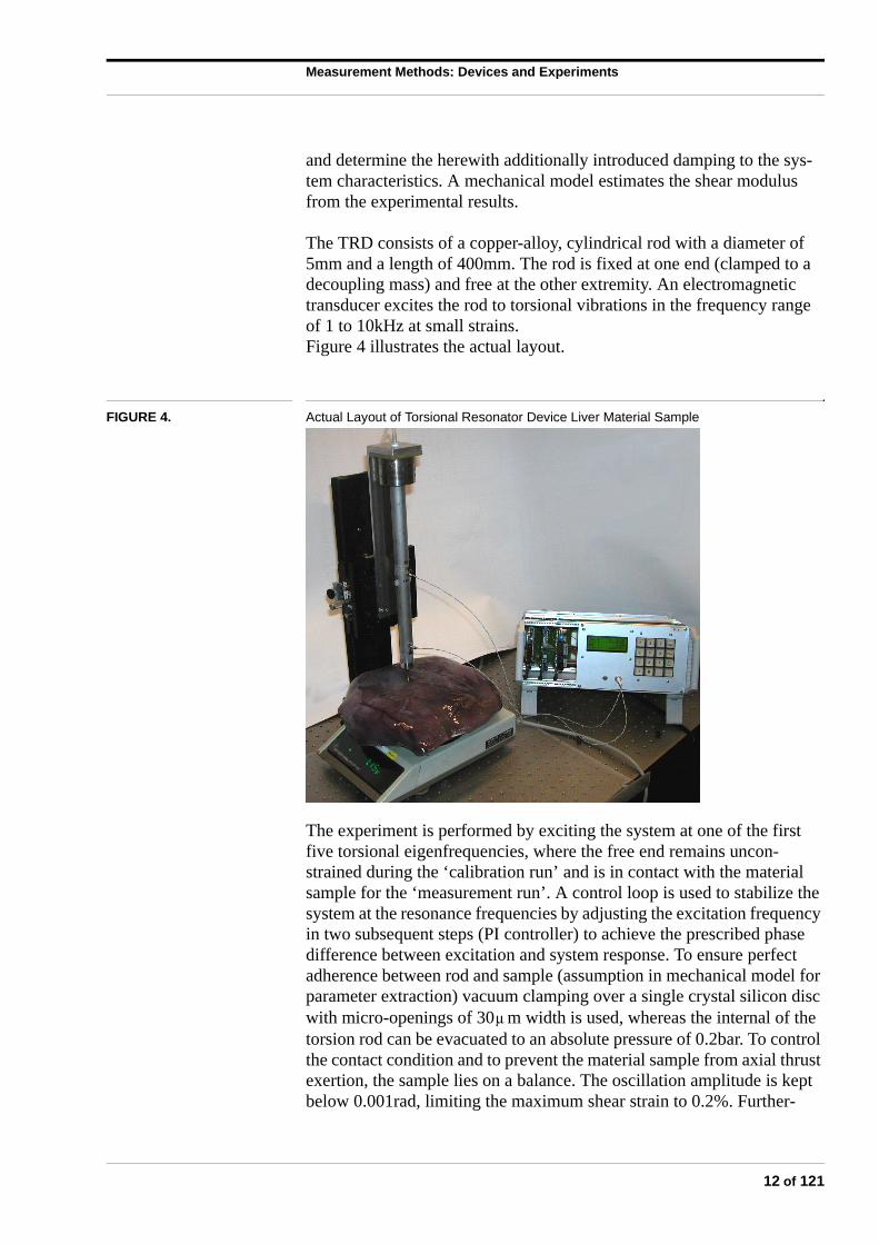
The TRD consists of a copper-alloy, cylindrical rod with a diameter of 5mm and a length of 400mm. The rod is fixed at one end (clamped to a decoupling mass) and free at the other extremity. An electromagnetic transducer excites the rod to torsional vibrations in the frequency range of 1 to 10kHz at small strains.Figure 4 illustrates the actual layout.

FIGURE 4. Actual Layout of Torsional Resonator Device Liver Material Sample

The experiment is performed by exciting the system at one of the first five torsional eigenfrequencies, where the free end remains uncon-strained during the ‘calibration run’ and is in contact with the material sample for the ‘measurement run’. A control loop is used to stabilize the system at the resonance frequencies by adjusting the excitation frequency in two subsequent steps (PI controller) to achieve the prescribed phase difference between excitation and system response. To ensure perfect adherence between rod and sample (assumption in mechanical model for parameter extraction) vacuum clamping over a single crystal silicon disc with micro-openings of 30 m width is used, whereas the internal of the torsion rod can be evacuated to an absolute pressure of 0.2bar. To control the contact condition and to prevent the material sample from axial thrust exertion, the sample lies on a balance. The oscillation amplitude is kept below 0.001rad, limiting the maximum shear strain to 0.2%. Further-

µ

12 of 121


more, a local characterization of the material is achieved due to the small

contact area (approx. 1cm3 material is measured).One experiment realization is typically of 1 minute duration and leads to several thousands oscillations at the characteristic frequencies, such that a steady-state harmonic response is reached in the system.

FIGURE 5. Schematic of Torsional Resonator Device Experiment

An analytical model of a torsional radiating source on a semi infinite space allows estimation of material parameters from the experimental results. Thereby the material is modelled as a linear viscoelastic, homog-enous and isotropic half space.The dynamic behavior of the overall system (oscillator and sample) is characterized by the complex transfer function around the excited reso-nance frequency, and is found by comparing the excitation signal with the response of the mechanical system.

(EQ 3)

Where in EQ 3 T* is the complex transfer function of the system, the resulting angular motion of the rod and M the exerted torque. In addition t and f represent time and frequency, respectively. Figure 6 shows a typi-cal transfer function of the system during calibration and measurement run. The phase curve of the transfer function, Arg(T*(f)), in turn exhibits two characteristical parameters of the system dynamics: the resonance frequency fres itself and the quality factor Q.

(EQ 4)

T∗ f( ) θ f t,( )M f t,( )----------------=

θ

Q2 π Um⋅ ⋅

D----------------------

fres

fd-------= =

13 of 121


(EQ 5)

FIGURE 6. Transfer Functions of the vibrating System: Calibration Run (TRD in Air) and Measurement Run (TRD in Contact with Tissue)

The quality factor is proportional to the ratio of maximum potential energy stored in the oscillating structure Um and the energy loss due to damping in one oscillation period D. This can be further expressed as ratio between resonance frequency fres and damping characteristic df, which are inferred from the control variables of the phase stabilization loop. The damping characteristic is determined from the difference of the

two measured frequencies fplus and fminus, corresponding to a phase shift difference of with respect to resonance frequency fres.

FIGURE 7. Resonance Frequency Shift and Quality Factor in Function of G* for the first Resonance Frequency (1300Hz)

fd fplus φ π2--- π

4---+ ⎠⎞ fminus φ π

2--- π

4---– ⎠⎞=⎝

⎛–=⎝⎛=

φ∆ π 4⁄±=

14 of 121


The required mechanical model of the experiment implies a classical tor-sion rod, shear-wave propagation (SH-polarization) in a linear visco-elastic half-space and the contact in-between as corresponding boundary condition to the particular problems. The semi-analytical solution allows to express the exerted torque as a function of the yet unknown material parameters of the sample, which in turn can be linked to the change in dynamic behavior of the resonator (increased damping and resonance fre-quency shift) when in contact (calibration run vs. measurement run). As seen above, the dynamic behavior of the system can be expressed equiva-lent by the characteristical and measured quantities Q and fres. Thus, in the final result of the analytical derivation (Valtorta et al. [18]), the mate-rial parameters and the system dynamics characteristical parameters Q and fres are linked one-to-one. Figure 7 shows the resulting relationships for the first resonance frequency. Finally thanks to this semi-analytical solution of the experiment, the unknown material parameters are directly linked to the experimental results (measurements of shifting in Q and fres between calibration and measurement run) and can be obtained from the mapping process.

Next the system is subject to harmonic boundary conditions up to the steady-state harmonic response of the system. Therewith the linear visco-elastic material parameters and the shear deformation are given by the classical description (representative: the complex frequency-dependant

shear modulus Ge* and shear deformation ):

(EQ 6)

and constitutive equation:

(EQ 7)

whereas

• shear strain

• shear stress

• angular frequency of the harmonic time function

• Ge1 real component of Ge*, storage modulus (elasticity)

• Ge2 imaginary component of Ge*, loss modulus (viscosity)

• phase of the modulus

• i basic imaginary unit

For soft tissues and relatively high frequencies, the wave propagation mainly takes place into the axial direction toward sample interior. Fur-thermore the attenuation of the SH-waves for stronger viscous materials

γ

Ge∗ ω( ) G

e 0( ) ei ω τ⋅ ⋅–

G·e τ( ) τd⋅

0

∞

∫+ G1e

i G2e⋅+ G

e∗ ei ϕ⋅⋅= = =

τ t( ) Ge∗ ω( ) γ t( )⋅=

γ

τ

ω

ϕ

15 of 121


leads to decreased amplitudes by one order of magnitude outside a layer of 3 or 4 times the torsional rod diameter. Therefore the half space model is justified for samples in which the distance between radiating source and sample boundaries are in the range of 1-2cm.

Generally, the standard deviation in determining |Ge*| and Ge1/Ge

2 of

synthetic materials with |Ge*| being larger than 50kPa is as low as 1%. Larger scatter is expected for lower absolute values of the shear modulus and for biological material.

The Torsional Resonator Device possess torsional eigenmodes at the sub-sequently listed frequencies, whereas no measurements are taken at the second eigenfrequency, since it is very close to a bending mode such that excitation of pure torsion cannot be achieved.

Eigenfrequencies of the TRD:

• 1st torsional resonance 1300Hz

• 3rd torsional resonance 6640Hz

• 4th torsional resonance 9310Hz

• 5th torsional resonance 12130Hz

The TRD technique implicates the advantage that no specific sample geometry is required (since the test piece is approximated as half space).

2.3 TeMPeST Test [22]

The Tissue Material Property Sampling Tool (TeMPeST 1-D) is a 12mm diameter minimally invasive instrument, designed to investigate visco-elastic properties of solid material under small deformations (in particu-lar solid organ tissue). A 5mm right circular punch vibrates the material surface while recording applied load and relative displacement. The declared instrument specifications are:

• range of motion

• position resolution

• maximal force to be exerted 300mN

• force resolution

• frequency range 0 - 200Hz (100Hz is the declared confidence limit)

The device can impose pure sinusodial, chirp (a form of frequency sweep), step and other load profiles.

The CIMIT Simulation Group provided data of a series TeMPeST tests on TC2 number 3 and 4.

500µm±

0.2µm±

70µN±

16 of 121


FIGURE 8. TeMPeST Device and Schematic

Given the ideal case of a linear elastic, isotropic, homogenous semi-infi-nite medium with known Poisson’s ratio , the Young’s modulus, or the Shear modulus respectively, can be resolved from the recorded force-rel-ative displacement response over the analytical exact solution of the infinitesimal, static normal indentation of a linear elastic half space by a rigid, circular flat punch (EQ 8 and cp. Johnson [5], Bycroft [37] and oth-ers):

(EQ 8)

and for incompressibility ( ):

(EQ 9)

where and P are the displacement and force normal to the surface, r0 is

the indenter radius and represents a correction factor for a medium of finite layer thickness h (cp. Hayes [33], paragraph 4.5). is unity for a semi-infinite body and increases with r0/h and /h.

FIGURE 9. Indentation of semi-infinite linear elastic Medium with rigid, right circular Punch and indicated finite Extent

ν

Ee P 1 ν2–( )⋅

2 r0 δz⋅ ⋅---------------------------=

Ge P 1 ν–( )⋅

4 r0 δz⋅ ⋅-------------------------=

ν 0.5=

Ee 38 r0⋅------------ P

δz

---- 1κ---⋅ ⋅=

δz

κκ

δz

2 r0

P

h

17 of 121


However, the TeMPeST-test is a dynamic small perturbation method around an initial static indentation (henceforth called ‘preload’). The pre-load is a necessary precondition so that positive contact between the vibrating indenter and the material sample is guaranteed throughout the test. With this procedure, the local gradient of the material characteristic

(stiffness) around the (finite) preload is measured ( ). EQ 9

becomes:

(EQ 10)

The static indentation formula is then extended to dynamics by making

the variables time-dependent and introducing a phase shift to include the detected phase difference between excitation and system response (damping, viscosity in medium):

(EQ 11)

where and denote the preload (static initial indentation). Finally, a frequency dependent, ‘complex’ modulus results:

(EQ 12)

where EQ 12 can be evaluated in the time domain or frequency domain. Evaluation in the frequency domain has the advantage, that in the case of a viscous tested material (theoretically) the actual observation period does not have to be a good deal longer than the relaxation time - instead very short observation periods are conceivable.It is to be emphasized, that the above represents only a ‘quasi’-extension to dynamics, as inertia within the system is not considered in this evalua-tion of the measurement data, respectively in the mechanical derivation of the evaluation formula.This can lead to an overestimation or underestimation of the modulus (depending if the excitation is the displacement or the force).This issue will be considered and investigated later on, along with effects and consequences of finite indentation (preload) and finite extent of the tested mechanical structure (in contrast to the assumed semi-infinite space).

Finally, for more sophisticated cases than the ideal case assumed above (e.g. material anisotropy, small structures, finite instead of the assumed infinitessimal instrument indentation along with nonlinear material

Ee

εddσ

=

Ee 38 r0⋅------------ Pd

δzd------- 1

κ---⋅ ⋅=

ei α⋅

δz δz δ+ z0 ei ω t⋅ ⋅⋅=

P P P+ 0 ei ω t α+⋅( )⋅⋅=

P δ

Ee∗ f( ) Ee∗ f( ) ei α⋅⋅=

Ee∗ f( ) 38 r0⋅------------

P0

δz0

------- 1κ---⋅ ⋅=

18 of 121


response, etc.) finite element models can be employed for appropriate data postprocessing, iteratively approaching the observed response by modifying the material parameters given the implied constitutive model (inverse FEM characterization of material) - even for hyperelastic mate-rial definitions.

2.4 Large-scale spherical Indentation Tests

The large-scale spherical indentation tests were performed by the CIMIT Simulation Group. CT-scans of the TC2s undergoing the large spherical indentation were provided.The experimental setup is given in figure 10 and 11. The TC2 rests on a no-slip plate. The experimental set-up loads then the TC2 under con-trolled boundary conditions, where a 2.54cm (1inch) diameter Delrin spherical indenter mounted on a 1.9cm diameter by 4.5cm long Delrin cylinder is loaded by a known force. A linear dial indicator measures the distance the spherical indenter is translated.To approximate a frictionless indentation boundary condition, the spheri-cal indenter was oiled.

FIGURE 10. Large-scale Indentation Tests: Test Setup by CIMIT Simulation Group

The TC2s exhibit randomly embedded fiducial markers (Teflon spheres) for CT trajectory tracking. To obtain a reference state of the internal sphere locations, the TC2 is initially imaged by a CT-scanner in the unloaded configuration. Then the procedure is repeated in the loaded configuration to capture the displacement field. The difference gives an approximation of the trajectories.

19 of 121


The test realizations include relative indentation (nominal strain) up to 30%.

FIGURE 11. Close-Up Schematic of spherical Indentation Situation

2.5 Classical Methods

2.5.1 Rheological Torsional Shear Test

The CIMIT Simulation Group provided data of a rheological torsional shear test on the used silicone rubber material. The test was performed on the AR2000 rheometer, TA Instruments. The following relevant specifi-cations are declared:

• torque range 0.1 Nm - 200mNm

• frequency range 7.5.10-7 - 628rad/s

• combined motor and transducer technology CMT

The test realizations include:

• frequency sweep at 5% and 20% shear strain 0 - 100Hz

• strain sweep at 0.1Hz 0 - 50% shear strain

The curves of force, position, strain, viscosity, velocity and frequency are given as direct output data of the rheometer in tabular form. However, the implied mechanical models are unknown. Since the test realizations include finite strains, potential improper modelling is investigated on the basis of the appropriate theory of finite elasticity in chapter 4.

2.5.2 Large-scale uniaxial Compression Test

The large-scale uniaxial compression test is performed at the Swiss Fed-eral Institute of Technology Zurich (ETHZ). This standard method of material testing was realized on a Zwick/Roell 1456 tension-compression testing machine. The curves of force and compression plate position are recorded. The following relevant specifications are declared:

• force resolution % of the effective force

• position resolution

µ

0.25±

3µm±

20 of 121


FIGURE 12. Zwick/Roell 1456: Tension-Compression Testing Machine and TC2 Cylinder disposed to Testing

The actual test setup is shown in figure 12. To prevent from shear trac-tions between compression plates and TC2 and thus approximate true uniaxial compression, the compression plates were oiled. Therewith the entire TC2 can freely and uniformly expand in lateral direction during compression. Figure 13 exhibits the fully compressed TC2. Buckling of the lateral surface is seen to be very small - demonstrating the TC2 in uniaxial state of stress. Furthermore, the compression speed is kept below 2mm/min. Therefore, the test can be assumed quasi-static.The test realizations include nominal compression up to 20%. A com-pression force of 0.01N indicated test initiation.

FIGURE 13. 20% nominal Compression of TC2 Cylinder, oiled Compression Plates

21 of 121


To give a further validation of the assumed Poisson’s number of (in addition to Aspiration Experiment), the TC2 volume change during compression is assessed optically using a high resolution camera captur-ing the contours of the undeformed and deformed cylinder. Image pro-cessing and analysis allows then to determine the relative volume change for the specified nominal compression with respect to the undeformed state.

ν 0.5=

22 of 121

Materials

3.0 Materials

3.1 Silicone Rubber

3.1.1 TruthCube2

Two special, cylindrical silicone phantoms named TruthCube2 (number 3 and 4) have been made available by the CIMIT Simulation Group. To dif-ferentiate them, they have 3 and respectively 4 radio-opaque markers on their top.Both TC2’s feature randomly embedded Teflon beads (fiducials, 1.58mm in diameter) for CT trajectory tracking during large-scale uniaxial com-pression and spherical indentation tests. 2% global softening of the syn-thetic specimens is expected due to the embedding of the fiducials [24].

The two-part, platinum-catalyzed silicone rubber material is the Ecoflex 0030 (Smooth-On), exhibits sticky surfaces and shows the dimensions:

• diameter 82.5mm

• height 82.3mm

The height was measured very accurately during the compression test, whereas the diameter was quantified by means of a sliding calliper with an estimated accuracy of .The silicone’s density is assessed by weighing the cubes and dividing by

their associated volume. A density of 1070kg/m3 is obtained, which is the same order of magnitude as for most biological tissues.Furthermore, the silicone can be assumed incompressible, as optically confirmed during the uniaxial compression test (cp. paragraph 5.1.2). The typical biological tissue is nearly incompressible due to the high water content.The above highlights, that such synthetic materials are in principle suit-able to emulate real biological tissues.

0.5mm±

23 of 121

Materials

FIGURE 14. TruthCube2 Number 4 Silicone Phantom underneath the Torsional Resonator Device

3.1.2 Constitutive Model

To mechanical model this silicone rubber material over a finite strain range, the neo-Hookean material formulation will be applied (hyperelas-ticity). It exhibits a more or less linear or even flattening force-elongation behavior in uniaxial tension, as does the silicone rubber. It will be shown in paragraph 5.1.2, that this silicone material is very well characterized by the neo-Hookean formulation.

The neo-Hookean strain energy function U has the following form:

(EQ 13)

where is the first deviatoric strain invariant and is a material param-eter. Parameter optimization against the uniaxial compression test deter-mines as 4908Pa.The concept of hyperelasticity is introduced in paragraph 4.

3.2 Liver

To account for the real behavior of biological tissue in the finite strain range, the FEM-investigation of the TeMPeST-experiment includes addi-tional simulations on liver material. Consequently a more application-oriented investigation is obtained.

3.2.1 Constitutive Models

The constitutive model and parameters for liver material are inferred from the aspiration experiment. A ‘soft’ and a ‘stiff’ liver are considered.

U µ I1 3–( )⋅=

I1 µ

µ

24 of 121

Materials

The energy strain function U is given in the fifth order reduced polyno-mial form (hyperelasticity):

(EQ 14)

is the first deviatoric strain invariant, J is the total volume change, Cn0 and D are the material parameters respectively and are given beneath. The liver material is taken as fully incompressible (D=0).

Liver 1 (soft):

• C10 883.8Pa

• C20 1707.9Pa

• C30 1449.9Pa

• C40 2691.8Pa

• C50 1757.5Pa

Liver 2 (stiff):

• C10 2255.9Pa

• C20 7017.4Pa

• C30 5027.2Pa

• C40 6194.6Pa

• C50 7494.2Pa

As mentioned, the concept of hyperelasticity will be introduced in para-graph 4.

U Cn0 I1 3–( )n 1

D---- J 1–( )2⋅+⋅

n 1=

5

∑=

I1

25 of 121

Theory, Derivations and Concepts

4.0 Theory, Derivations and Concepts

4.1 Theory of finite Elasticity [17]

Mechanical and geometric nonlinearities require the theory to be obtained without any approximations, such as the classical made linear-izations in the infinitesimal strain range. Consequently the theory becomes exact.Accurate description of general material elasticity is realized in this work by the concept of hyperelasticity. An elastic material for which a strain-energy function exists is called a ‘Green elastic’ or ‘hyperelastic’ mate-rial. The mechanical properties of a hyperelastic material are character-ized, respectively modeled, in the strain-energy function (constitutive modeling).

4.1.1 Exact Kinematics

Since the kinematics will be obtained without any approximation, they are exact and are sometimes referred to as ‘finite strain measures’. On this geometric linear algebra provides the analytical basis.

Configurations. The deformation of continuous bodies are seen only in their configurations in the Euclidean three-dimensional space. A distinc-tion is drawn between ‘present’ and ‘reference’ configuration.The ‘present configuration’ of the body is defined by its position vector x identifying the place occupied by a particle Y at the present time t (small letters).It is convenient to refer everything concerning the body’s deformation and motion to one particular configuration, called the ‘reference configu-ration’. The reference configuration is given by the position vector X of particle Y (capital letters), and doesn’t have to occupy necessarily an actual nor the initial body configuration. Nota bene that the reference configuration does not depend on time as it is a single constant configura-tion.

(EQ 15)

In what for instance applies: I=X, Y, Z and i=x, y, z for a rectangular Car-tesian coordinate system. eI is the constant orthonormal basis associated with the reference configuration, and ei is the constant orthonormal basis associated with the present configuration. Usual summation convention over repeated indices is to be used (Einstein’s summation convention).Usually it is sufficient to let these basis coincide, so that . The

bold dot denotes the scalar product, is the usual Kronecker delta sym-bol.

Mapping Relation. The mapping relation from the reference configuration to the present configuration (EQ 15) specifies how each particle Y of the

X XI eI⋅= x xi ei⋅=

ei eI• δiI=

δiI

26 of 121


body moves through space as time progresses (i.e. motion and deforma-tion).

(EQ 16)

Deformation Measures. To describe the deformation of the body from the reference configuration to the present configuration the following defor-mation measures are defined:

The ‘deformation gradient’ F gives the incremental deformation of a material line element dX in the reference configuration to the material line element dx in the present configuration:

(EQ 17)

Thus it appears that the mapping of each line element from the reference configuration to the present configuration is given by:

(EQ 18)

so that the deformation gradient F characterizes the dilatation (volume change) and distortion (shape change) of a material element from the ref-erence configuration to the present configuration. In Cartesian coordi-nates the deformation gradient tensor F is found as:

(EQ 19)

and consequently in cylindrical coordinates:

(EQ 20)

with x, y, z and X, Y, Z representing the rectangular coordinates in the present and reference configuration, and equally r, , z and R, , Z being the cylindrical coordinates in the present and reference configuration in radial, circumferential and axial direction, respectively.

x f X t( , )=

F ∂x∂X-------=

dx FdX=

F

∂x∂X------ ∂x

∂Y------ ∂x

∂Z------

∂y∂X------ ∂y

∂Y------ ∂y

∂Z------

∂z∂X------ ∂z

∂Y------ ∂z

∂Z------

=

F

∂r∂R------ ∂r

R ∂Θ⋅--------------- ∂r

∂Z------

r ∂θ⋅∂R

------------- r ∂θ⋅R ∂Θ⋅--------------- r ∂θ⋅

∂Z-------------

∂z∂R------ ∂z

R ∂R⋅--------------- ∂z

∂Z------

=

θ Θ

27 of 121


The definition of the ‘right Green deformation tensor’ C arises from the derivation of the magnitude ds of the material line element dx in the present configuration:

(EQ 21)

what yields for convenience the right Green deformation tensor:

(EQ 22)

It is also convenient to give the ‘left Green deformation tensor’ B:

(EQ 23)

The ratio between the lengths ds and dS of an arbitrary line element in the present and reference configuration, respectively, results in the general definition of the ‘stretch’:

(EQ 24)

Where the associated extension E of the material line element is given as:

(EQ 25)

An extension of a material line element relative to its reference length involves a stretch greater than one.

An arbitrary ‘elemental material volume’ is defined by its adherent line

elements dX1, dX2, dX3 in the reference configuration (dV), and by the

associated line elements dx1, dx2, dx3 in the present configuration (dv).

(EQ 26)

Where the cross in EQ 26 denotes the vector product (cross product). The ratio of the elemental volumes dv and dV is the ‘relative volume change of the material element’ J. After several basic linear algebraic manipula-tions and using the mapping relation in EQ 18, a fundamental and well-known linear algebraic expression is found for the relative volume change of a material element:

(EQ 27)

One recognizes at once the elemental material volume in the reference configuration dV in the last expression of EQ 27. It follows:

ds( )2dx dx• FdX FdX• dX FTFdX• dX CdX•= = = =

C FTF=

B FFT=

λ dxdX---------- ds

dS------= =

E λ 1–=

dV dX1dX2× dX3•= dv dx1

dx2× dx3•=

dv FdX1 FdX2× FdX3• det F( )F T–dX1

dX2×( ) FdX3•= =

det F( ) dX1dX2×( ) F 1–• FdX3= det F( )dX1

dX2dX3•×=

28 of 121


(EQ 28)

and finally the relative volume change of a material element is obtained as:

(EQ 29)

This means that J is a pure measure of dilatation. Another pure measure of dilatation can be derived based on the right Green deformation tensor C, rather than on the entirely equivalent deformation gradient tensor F. The resultant scalar I3 becomes:

(EQ 30)

To measure the ‘shape change of a material element’, the deformation

gradient F is separated into its dilatational part J1/3.I (cp. EQ 31) and its distortional part F’:

(EQ 31)

in which I is the identity matrix. Whenever the determinant J is equal to unity, the material element maintains its original volume and is only dis-torted. Consequently F’ is a pure measure of distortion. Nota bene that F’ is in general not deviatoric.

The strain measures are found in the derivation of the change in length of a line element:

(EQ 32)

what allows to yield the ‘Lagrangian strain tensor’ E as:

(EQ 33)

The Lagrangian strain tensor can also be expressed with the ‘displace-ment vector’ u. The displacement vector u is the vector that connects the position X of a material point in the reference configuration to its position x in the present configuration:

(EQ 34)

From the definition of the deformation gradient F (EQ 17) follows:

(EQ 35)

Introducing the right Green deformation tensor C (EQ 22) gives:

dv det F( ) dV⋅ J dV⋅= =

J det F( )=

I3 det C( ) J2= =

F J1 3⁄ I⋅( )F′=

ds( )2dS( )2– dX C I–( )• dX dX 2 E⋅( )• dX= =

2 E⋅ C I–=

u x X–=

F ∂x∂X------- ∂ X u+( )

∂X--------------------- I ∂u

∂X-------+= = =

29 of 121


(EQ 36)

With EQ 33 the well-known definition of the Lagrangian strain is received:

(EQ 37)

or in index notation:

(EQ 38)

whereas the comma denotes a derivative with respect to the coordinate that follows.For small deformations the Lagrangian strain tensor E passes into the classical strain tensor used in linear continuum mechanics:

(EQ 39)

The associated stretches are found by simply adding one to the corre-sponding material line element extensions ( , cp. EQ 25 & EQ 38):

(EQ 40)

To complete the deformation measures, the three ‘invariants of the state of strain’ are given.Since the Lagrangian strain tensor E and the right Green deformation ten-sor C are closely related, the subsequent relation holds:

(EQ 41)

The invariants of the right Green deformation tensor C are:

(EQ 42)

(EQ 43)

(EQ 44)

C FTF I∂u∂X-------+⎝ ⎠

⎛ ⎞T

I∂u∂X-------+⎝ ⎠

⎛ ⎞ I∂u∂X------- ∂u

∂X-------⎝ ⎠⎛ ⎞

T ∂u∂X-------⎝ ⎠⎛ ⎞

T ∂u∂X-------⎝ ⎠⎛ ⎞+ + += = =

E12--- ∂u

∂X------- ∂u

∂X-------⎝ ⎠⎛ ⎞

T ∂u∂X-------⎝ ⎠⎛ ⎞

T ∂u∂X-------⎝ ⎠⎛ ⎞+ +⋅=

Eij12--- ui j, uj i, uk i, uk j,⋅+ +( )⋅=

εij12--- ui j, uj i,+( ) Eij≈⋅=

Eij i j=

λi Eij i j=1+

12--- ui j, uj i,+( )⋅

i j=

1+= =

Eij∂∂

2Cij∂∂⋅=

I1 C I• B I• Cii Bii= = = =

I212--- C I•( )2 C C•–[ ]⋅ 1

2--- B I•( )2 B B•–[ ]⋅= =

12--- I1( )2

Cij Cij⋅–[ ]⋅=12--- I1( )2

Bij Bij⋅–[ ]⋅=

I3 det C( ) det B( ) J2= = =

30 of 121


The invariants of the deformation gradient tensor F (correspond to the so-called reduced invariants of the right Green deformation tensor C) become:

(EQ 45)

(EQ 46)

(EQ 47)

4.1.2 Constitutive Equations - Hyperelasticity

Constitutive equations characterize the mechanical response of a given material to deformations and deformation rates. They are given here in the context of pure mechanical theory and for hyperelastic materials. The concept of hyperelasticity is appropriate for the general case of nonlinear elastic solids up to finite deformations. An elastic solid exhibits ideal behavior in the sense, that it has no material dissipation and is character-ized by a strain energy function. The same applies to the concept of hyperelasticity: the energy stored in a deformed hyperelastic material is independent of the deformation path (no hysteresis) and is solely deter-mined by the analytic formulation of a ‘strain energy function’ U (consti-tutive modeling) - whereas the virtual work principal is used to obtain the internal energy variation.

Stress-Strain relationships and Stress Tensors. The stress-strain relationships of any work conjugate stress and strain measures are then obtained by derivatives of the strain energy function U:

(EQ 48)

whereas T is the ‘Cauchy stress tensor’ (true stresses). The engineering (nominal) stresses are found in the ‘second Piola-Kirchhoff stress tensor’ S as:

(EQ 49)

Stress can be understood as a force acting per unit area. In this context the ‘true stress’ refers to a force per unit area in the present configuration. Other than the ‘engineering stress’ (nominal stress), which is a force act-ing in the present configuration, but measured with respect to the refer-ence configuration, per corresponding unit area.The relation between true and engineering stress is specified by:

(EQ 50)

I1 I31 3⁄–

I1⋅=

I2 I32 3⁄–

I2⋅=

J I3 det F( ) det C( )[ ]1 2⁄= I3= = =

T 2 F∂U∂C-------FT⋅=

S∂U∂E------- 2

∂U∂C-------⋅= =

t n( ) adS∫ s N( ) Ad

S0

∫=

31 of 121


with t being the force vector per unit area in the present configuration (true stress), s the force vector with respect to the reference configuration (engineering stress), dA the element of area in the reference configuration with its unit outward normal N and da the element of area in the present configuration with unit outward normal n. S and S0 denote the associated material part in present and reference configuration, respectively.With EQ 50 results the following relation between the Cauchy stress tensor T and second Piola-Kirchhoff stress tensor S:

(EQ 51)

The stress tensor can be separated into their spherical and deviatoric parts. For the Cauchy stress tensor T follows:

(EQ 52)

and

(EQ 53)

where T’ is the deviatoric part, -p.I the spherical part and p by itself the pressure (hydrostatic pressure stress) of the respective Cauchy stress ten-sor T.

The isotropic, nonlinear elastic Material. It can be shown that if an elastic material is isotropic in its reference configuration, its strain energy func-tion U is a function of the three invariants of the state of strain solely:

(EQ 54)

or in terms of the reduced invariants:

(EQ 55)

Consequently the corresponding stress tensors become as well a function of the state of strain solely, and can be expressed in terms of the strain invariants in the following way:

(EQ 56)

(EQ 57)

When a material is fully incompressible, U remains as a function of the first and second strain invariants only. Furthermore, for the specific case of incompressibility the total pressure p is no longer determined by a con-

T J1– FSFT⋅=

T p I T′+⋅–=

p13--- T I•⋅–=

U U I1 I2 I3,( , )=

U U I1 I2 J,( , )=

T 2 J 1– ∂U∂I1

------- B I•( ) ∂U∂I2

-------⋅+ B 2 J 1– ∂U∂I2

------- B2 ∂U∂J------- I+⋅ ⋅–⋅ ⋅=

S 2∂U∂I1

------- C I•( ) ∂U∂I2

-------⋅+ I 2∂U∂I2

------- C∂U∂J------- J C 1–⋅ ⋅+⋅–⋅=

32 of 121


stitutive equation (e.g. any arbitrary hydrostatic pressure on an incom-pressible, isotropic material will not change the deformation). In the FEM-language this phenomenon is known as ‘locking’.Given this problem associated with nearly or totally incompressible materials, FEM-codes use mixed formulations (also known as hybrid for-mulation) of the elements. Mixed formulations of the elements use both displacement and pressure degrees of freedom. To separate the hydro-static pressure from the stress tensor, the following strain energy function is used:

(EQ 58)

where UH represents a hydrostatic work term. The stresses resulting from Û are deviatoric. While UH is the only term which contributes to the hydrostatic pressure in the material:

(EQ 59)

Material Models - Forms of the Strain Energy Potential. It is assumed, that the strain-energy U and the stress tensor T vanish in the undeformed state,

where , and , such that:

(EQ 60)

Given this and that the elastic material is isotropic in its reference config-uration, the following materials have been used in this work:

The neo-Hookean form:

(EQ 61)

where U is the strain energy per unit of reference volume, and D are the material parameters respectively. The neo-Hookean material is a spe-cial case of the subsequent reduced polynomial form (N=1)

The reduced polynomial form:

(EQ 62)

where U is the strain energy per unit of reference volume, N the order of the reduced polynomial form and Cn0 and D are the material parameters respectively.

U U I1 I2,( ) UH J( )+=

p∂UH

∂J----------–=

I1 3= I2 3= J 1=

U 3 3 1, ,( ) 0= T 0=

U µ I1 3–( ) 1D---- J 1–( )2⋅+⋅=

µ

U Cn0 I1 3–( )n 1

D---- J 1–( )2⋅+⋅

n 1=

N

∑=

33 of 121


The reduced polynomial form can be interpreted as a general polynomial series extension to the classic and well known neo-Hookean material.

By setting D to zero, the neo-Hooekan and reduced polynomial materials are obtained as fully incompressible (where throughout is a direct consequence, but is likewise a mathematically necessary constraint).

So far, the dependency of the strain-energy function U on the second

strain invariant has been neglected (accentuated by the attribute ‘reduced’). This is a common procedure and is justified since it can be shown that the sensitivity of U to changes in the second strain invariant is generally much smaller than the sensitivity to changes in the first strain invariant. In addition, the second strain invariant dependency of U is hard to measure.

Generalized Blatz-Ko material:

(EQ 63)

where U is the strain energy per unit of reference volume and the material

parameters are directly given as classic engineering parameters: is the well-known Lamé constant (shear modulus), is the Poisson’s ratio and f measures the volume fraction of voids in the material ( ).The Blatz-Ko material is in particular suitable for rubber and foam-rub-ber materials. By setting f=0 the Blatz-Ko material for non-foamed mate-rials is obtained:

(EQ 64)

Taking the limit of EQ 64 as the Poisson’s ratio approaches 0.5 allows to obtain the incompressible formulation of the Blatz-Ko material:

(EQ 65)

Linearization of the hyperelastic constitutive Equations. Linearization of the hyperelastic material formulations in the undeformed configuration allows to convert material parameters to their initial, linear elastic mod-ules, which are the classic engineering parameters. These parameters are

J 1=

I2

Uµe

2----- f I1 1–

1ν---–

1 2 ν⋅–( )ν

------------------------ I3( ) ν 1 2 ν⋅–( )⁄–⋅+⎩ ⎭⎨ ⎬⎧ ⎫

…+⋅ ⋅=

… µe

2-----+ 1 f–( )

I2

I3

---- 1–1ν---–

1 2 ν⋅–( )ν

------------------------ I3( )ν 1 2 ν⋅–( )⁄⋅+⎩ ⎭⎨ ⎬⎧ ⎫

⋅ ⋅

µe

ν0 f 1≤ ≤

Uµe

2-----

I2

I3

---- 1–1ν---–

1 2 ν⋅–( )ν

------------------------ I3( )ν 1 2 ν⋅–( )⁄⋅+⎩ ⎭⎨ ⎬⎧ ⎫

⋅=

ν

Uµe

2-----

I2

I3

---- 1–1ν---–

1 2 ν⋅–( )ν

------------------------ I3( )ν 1 2 ν⋅–( )⁄⋅+⎩ ⎭⎨ ⎬⎧ ⎫⋅

ν 0.5→lim

µe

2-----

I2

I3

---- 3–⎝ ⎠⎛ ⎞⋅= =

34 of 121


more intuitive and provide a proper basis for comparison of material parameters originating from different constitutive models.

In the case of polynomial strain-energy functions, linearization can be achieved by neglecting higher order terms. Comparison of coefficients with the linear elastic, isotropic constitutive equations then yields the ini-

tial shear modulus Ge, the Poisson’s number and consequently the ini-

tial Young’s modulus Ee.A more generally applicable and mathematical sound procedure is to derive the limit of the considered constitutive equations as the strains tend to zero and then compare to the linear elastic, isotropic material law. This procedure is presented underneath in index notation:

Firstly, the general second Piola-Kirchhoff stresses are computed against the material parameters by including the energy-strain function of the considered hyperelastic material. Nota bene that it is irrelevant which stress measure is implied, since for infinitessimal small strains applies!

(EQ 66)

For the neo-Hookean material is obtained, using Mathematica 5.0:

(EQ 67)

The constitutive equation for the second Piola-Kirchhoff stresses can be linearized by taking the local derivative with respect to the Lagrangian strains in the undeformed state:

(EQ 68)

where Cijkl is the fourth order tensor of the 21 material parameters of lin-ear elasticity, and can now be obtained directly by derivating the second Piola-Kirchhoff stresses with respect to the Lagrangian strains. By means of Mathematica 5.0, the following is found:

ν

T S≈

Sij∂U

∂I1

------- 2 I31 3⁄– δi j

13--- I1 Cij

1–⋅ ⋅–⎝ ⎠⎛ ⎞ …+⋅ ⋅ ⋅=

… ∂U

∂I2

------- 2 I32 3⁄– I1 δij Cij–

23--- I2 Cij

1–⋅ ⋅–⋅⎝ ⎠⎛ ⎞ ∂UH

∂J---------- J Cij

1–⋅ ⋅+⋅ ⋅ ⋅+

Sij2 J⋅

D C⋅ i j

---------------–J

2 2⋅D C⋅ ij

---------------2 δi j µ⋅ ⋅

I31 3⁄

---------------------2 I1 µ⋅ ⋅

3 Cij I31 3⁄⋅ ⋅

----------------------------–+ +=

dSij

∂Sij

∂Ekl

---------- dEkl⋅ Cijkl dEkl⋅= = Cijkl

∂Sij

∂Ekl

----------=

35 of 121


(EQ 69)

In the case of undeformed, isotropic material configuration, the following applies:

(EQ 70)

(EQ 71)

Cijkl in terms of the neo-Hookean material (EQ 61) reduces to:

(EQ 72)

In linear isotropic elasticity Cijkl is given as follows:

(EQ 73)

whereas and are the Lamé constants, which in turn are in classical representation:

(EQ 74)

Comparing coefficients (EQ 72, EQ 73 and EQ 74) yields finally the sought-

after conversion to the initial shear modulus Ge, the Poisson’s number

and consequently the initial Young’s modulus Ee of the neo-Hookean material parameters in the undeformed configuration:

(EQ 75)

Furthermore, the material parameter D can be expressed in terms of the well-known ‘bulk modulus’ . The bulk modulus is defined as the ratio of the hydrostatic normal stress p, to the associated unit volume change e. Within the limits of linear isotropic elasticity, the last two equals signs in EQ 76 hold:

(EQ 76)

Cijkl1

9 Cij Cik Ckl Clj I33⋅ ⋅ ⋅ ⋅ ⋅

--------------------------------------------------------------- 9 2( Cij Ckl J 1–( ) …+⋅ ⋅ ⋅⋅–(⋅=

… Cik Clj 1 2 J⋅–( ) ) J2D---- I3

3 4 3 Cik Clj Cij δi j Ckl δkl⋅+⋅( )⋅ ⋅ ⋅( ) …–⋅–⋅ ⋅ ⋅ ⋅ ⋅+

… 3 Cij Ckl Cik Clj⋅+⋅ ⋅( ) I33 I1 ) µ }⋅ ⋅ ⋅–

Cij Cij1– δij= =

I1 3= I2 3= J 1=

Cijkl2D---- 4 µ⋅

3----------–⎝ ⎠

⎛ ⎞ δij δkl 4 µ δik δjl⋅ ⋅ ⋅+⋅ ⋅=

Cijkl λe δi j δkl 2 µe δik δj l⋅ ⋅ ⋅+⋅ ⋅=

λe µe

λe ν Ee⋅

1 ν+( ) 1 2 ν⋅–( )⋅----------------------------------------------= µe E

e

2 1 ν+( )⋅------------------------ Ge= =

ν

µe 2 µ⋅= Ee 18 µ⋅

3 D µ⋅+---------------------= ν 3 2 D µ⋅ ⋅–

2 3 D µ⋅+( )⋅----------------------------------=

κ κ

κ pe--- λe 2

3--- µe⋅+

2 µe 1 ν+( )⋅ ⋅3 1 2 ν⋅–( )⋅----------------------------------= = =

36 of 121


Hence, the material parameter D is given as (comparison of coefficients, EQ 74 through EQ 76):

(EQ 77)

and likewise:

(EQ 78)

By either taking the limits of EQ 74 through EQ 77 as the Poisson’s number goes to 0.5 or taking the limit of EQ 78 as the bulk modulus tends to

infinity, the totally incompressible case of the converted neo-Hookean material parameters is derived:

(EQ 79)

In this limiting case, the material parameter D becomes zero, as indicated previously.

The following index notation derivatives have been used:

The derivatives of the three strain invariants with respect to the compo-nents of the Lagrangian strain tensor Eij:

(EQ 80)

(EQ 81)

(EQ 82)

The derivatives of the three reduced strain invariants with respect to the components of the Lagrangian strain tensor Eij:

(EQ 83)

(EQ 84)

(EQ 85)

D2κ---=

Ee 18 µ κ⋅ ⋅

3 κ⋅ 2 µ⋅+----------------------------= ν 3 κ⋅ 4 µ⋅–

6 κ 4+ µ⋅ ⋅----------------------------=

υ κ

Ee

ν 0.5→κ ∞→

lim 6 µ⋅ 3 µe⋅= = Ge 2 µ⋅ µe= =

∂I1

∂Eij

--------- 2 δi j⋅=

∂I2

∂Eij

--------- 2 I1 δi j Cij–⋅( )⋅=

∂I3

∂Eij

--------- 2 I3 Cij1–⋅ ⋅=

∂I1

∂Eij

--------- 2 I31 3⁄– δij

13--- I1 Cij

1–⋅ ⋅–⎝ ⎠⎛ ⎞⋅ ⋅=

∂I2

∂Eij

--------- 2 I32 3⁄– I1 δ⋅ i j Cij–

23--- I2 Cij

1–⋅ ⋅–⎝ ⎠⎛ ⎞⋅ ⋅=

∂J∂Eij

--------- J Cij1–⋅=

37 of 121


The derivative of the reciprocal components of the right Green deforma-tion tensor Cij with respect to the components of the Lagrangian strain tensor Ekl:

(EQ 86)

Using again Mathematica 5.0, the same procedure was applied to the 5th order reduced polynomial form, but results in a rather cumbersome deri-vation.For incompressible behavior (D=0), an analog parameter conversion is found as for the incompressible neo-Hookean material (parameters from higher order terms drop out):

(EQ 87)

As regards the Blatz-Ko material, the parameters are already the initial

shear modulus and the Poisson’s number , respectively.

4.1.3 Equilibrium of the Continuum and Boundary Conditions

Within the context of the purely mechanical theory, the local equilibrium of linear momentum prescribes how a particle Y comprised by any con-tinuous body moves through space and time. These are the purely contin-uum mechanical equations of motion and deformation and represent the equilibrium laws of the continuum.

Equilibrium Laws of the Continuum. Each particle Y of the continuum must satisfy Newton’s law of motion. This gives rise to the local form of the equilibrium of linear momentum (Cauchy’s equations of motion):

(EQ 88)

in what T is the Cauchy stress tensor, the effective local mass density, b the body force per unit mass vector and a the local particle acceleration:

(EQ 89)

In the most general case all of these quantities are dependent on time. If the time-dependence, and in particular the acceleration, vanishes EQ 88 reduces to the static equilibrium equations of linear momentum:

(EQ 90)

Finally, in the absence of body forces the divergence of the Cauchy stress tensor T remains, that is the primitive stress equilibrium:

(EQ 91)

∂Cij1–

∂Ekl

----------- 2 Cik1– Clj

1–⋅ ⋅–=

Ge 2 C10⋅= E

e 6 C10⋅=

µe ν

div T( ) ρ b⋅+ ρ a⋅=

ρ

a x·· u··= =

div T( ) ρ b⋅+ 0=

div T( ) 0=

38 of 121


The components of the divergence of the Cauchy stress tensor T are:

Rectangular coordinates:

(EQ 92)

(EQ 93)

(EQ 94)

Cylindrical coordinates:

(EQ 95)

(EQ 96)

(EQ 97)

with x, y, z representing the rectangular coordinates in the present config-uration, and equally r, , z being the cylindrical coordinates in the present configuration in radial, circumferential and axial direction, respectively. That is why EQ 95 through EQ 97 are sometimes denoted as radial, circumferential and axial equilibrium.It is to be noted that for symmetric stress tensor: must apply.

Boundary Condition for the Stress Tensor. The general form of the local equi-librium of linear momentum consists of a system of partial differential equations, which require both initial and boundary conditions.In the case of steady-state conditions and absent body forces, the only nontrivial condition is the stress boundary condition at the body’s sur-face. This boundary condition requires the body to counteract the exter-nal surface tractions. The stress boundary condition is given as:

(EQ 98)

where n is the unit outward normal vector to the boundary, T is the stress tensor evaluated at the boundary and t is the force vector per unit area on the boundary. denotes the surface of body P.

For analytic problem investigation the above provides basis for the com-plete determination of prescribed deformation field ansatz functions by finding the equilibrium configurations!

div T( )( )x

∂Txx

∂x----------

∂Txy

∂y----------

∂Txz

∂z----------+ +=

div T( )( )y

∂Tyx

∂x----------

∂Tyy

∂y----------

∂Tyz

∂z----------+ +=

div T( )( )z

∂Tzx

∂x----------

∂Tzy

∂y----------

∂Tzz

∂z----------+ +=

div T( )( )r

∂Trr

∂r---------- 1

r---

∂Trθ

∂θ-----------⋅

Trr Tθθ–

r---------------------

∂Trz

∂z----------+ + +=

div T( )( )θ∂Tθr

∂r----------- 1

r---

∂Tθθ

∂θ-----------⋅

Trθ Tθr+

r---------------------

∂Tθz

∂z-----------+ + +=

div T( )( )z

∂Tzr

∂r---------- 1

r---

∂Tzθ

∂θ-----------⋅

∂Tzz

∂z----------

Tzr

r-------+ + +=

θ

Trθ Tθr– 0=

t Tn( ) ∂P=

∂P

39 of 121


4.2 Analytical Investigation of the Rheological Torsional Shear Test

Description of the rheometer and the test setup are give in paragraphs 2.3.1 and 5.1.1. The shear test is analytically investigated by means of continuum mechanics approach, including the classical theory as well as the theory of finite elasticity.

FIGURE 15. Assumed Test Setup and Coordinate System

4.2.1 Classical Theory

The following theoretical cases are distinguished:

• linear elastic with quasi-dynamic extension

• linear elastic, dynamic

• linear viscoelastic, dynamic

General assumptions:

• right-circular cylindrical test piece: homogeneous, isotropic, linear elastic contin-uum

• perfect contact between test piece and excitation plates (no slip)

• pure torsion: exerted external axial thrust negligible

• lateral surfaces traction-free

• no body forces

In consequence, the cylindrical test piece is modeled as classical torsion rod.

Linear elastic, quasi-dynamic Model. The torsional shear stress is given by the following constitutive equation:

(EQ 99)

where the shear stress and strain are simply denoted by and for con-venience. The appropriate shear stress distribution in the circular cross sections is linear with radius and follows from:

excitation plate

material sampler

z

ϑ z t,( ) T t( ),

R0 hno slip boundary conditions

τϕz τ 2 Ge εϕz⋅ ⋅ 2 G

e ε⋅ ⋅= = =

τ ε

40 of 121


(EQ 100)

with , T and Wp being the specific torsion angle, the measured tor-sional moment and the polar section modulus, respectively:

(EQ 101)

Ip is the polar geometrical moment of inertia, and derived as subsequent for a circular cross section:

(EQ 102)

The specific torsion angle can be estimated as:

(EQ 103)

Harmonic excitation is introduced by:

(EQ 104)

Whereas the oscillating torque is found as:

(EQ 105)

where is the detected phase shift between excitation and system response. For phase shifts different from zero, the shear modulus becomes a complex quantity and indicates viscous behavior (damping) in the mechanical system. Thus, in general the shear modulus must be spec-

ified as complex shear modulus Ge*:

(EQ 106)

As is the in-phase storage modulus, is the out-of-phase loss modu-

lus and is the phase of the complex shear modulus (cp. EQ 6 & EQ 7).

Altogether allows to solve for the complex shear modulus Ge* as func-tion of the applied torsion angle and the measured torque T:

(EQ 107)

This is the complex transfer function of the modeled mechanical system. Nota bene that inertia has been neglected so far, since this derivation was

τ TIp

---- r⋅ TWp R0⋅----------------- r⋅ Ge ϑ z, z( ) r⋅⋅= = =

ϑ z, z( )

Wp

Ip

R0

-----=

Ip r2

Sd⋅∫∫ π d4⋅32

-------------= =

ϑ z,

ϑ z( )z h=

h----------------------=

ϑ z h= t,( ) ϑ0 ei ω t⋅ ⋅⋅=

T t( ) T0 ei ω t α+⋅( )⋅⋅=

αα

Ge∗ G1

eG2

ee

i ϕ⋅⋅+=

G1e G2

e

ϕ

ϑ h t,( )

Ge∗ T t( )Ip ϑ z, t( )⋅---------------------- h

Ip

----T0

ϑ0

------ ei α⋅⋅ ⋅= =

41 of 121


based on static equations. This is accentuated by the term ‘quasi-dynamic’! Consequently resonances are not detected from these equa-tions.

Linear elastic, dynamic Model. Effects of inertia are included by the subse-quent governing equation of the classical torsional resonator:

(EQ 108)

where is the mass density and cs is the secondary wave speed (shear wave speed):

(EQ 109)

The torsion rod is subject to the following boundary conditions:

(EQ 110)

is the torsional amplitude. The first boundary condition is the system excitation, the second boundary condition is the clamped bottom of the test piece. The general solution for EQ 108 is the steady-state harmonic function of EQ 111 in the case of steady-state condition and harmonic exci-tation:

(EQ 111)

as bracketed term represents the axial distribution of the oscillation amplitude, A and B are problem constants and k is the wave number:

(EQ 112)

By satisfying the boundary conditions in EQ 110, the oscillation EQ 111 can be determined as:

(EQ 113)

Finally the complex shear modulus Ge* is found in respect of the excita-tion and the measured torque T:

(EQ 114)

ϑ t t, cs ϑ zz,⋅ Ge

ρ------ ϑ zz,⋅= =

ρ

csG

e

ρ------=

ϑ h t,( ) ϑ0 ei ω t⋅ ⋅⋅=

ϑ 0 t,( ) 0=

ϑ0

ϑ z t,( ) A k z⋅( ) B k z⋅( )cos⋅+sin⋅[ ] ei ω t⋅ ⋅⋅=

kωcs

----=

ϑ z t,( )ϑ0

k h⋅( )sin---------------------- k z⋅( ) e

i ω t⋅ ⋅⋅sin⋅=

ϑ h t,( )

Ge∗ 1

Ip

---- T t( )ϑ z, z t,( )

z h=

-----------------------------⋅ k h⋅( )tanIp k⋅

-----------------------T0

ϑ0

------ ei α⋅⋅ ⋅= =

42 of 121


The linear elastic, dynamic solution differs from the quasi-dynamic solu-

tion by a factor .

Resonance frequencies are found for:

(EQ 115)

n is the mode of torsional resonance. Thus results for the resonance fre-quency fres:

(EQ 116)

whereas the angular frequency is defined as:

(EQ 117)

The respective wave lengths are computed, to be compared with the char-acteristic dimension of the test piece (important to justify or reject the use of the classical theory):

(EQ 118)

Linear viscoelastic, dynamic Model. To account in addition for viscous behavior in the torsion rod within the scope of classic linear viscoelastic-ity theory, the wave EQ 108 is transformed by means of the correspondence principle:

(EQ 119)

where the encircled cross denotes a convolution product. When introduc-ing the following ansatz function for a forced oscillation:

(EQ 120)

EQ 119 reduces to an ordinary differential equation for the complex torsion angle amplitude function :

(EQ 121)

In consequence of EQ 121, a complex shear wave speed cs*, a complex

wave length and so a complex wave number k*:

(EQ 122)

k h⋅( )tank

-----------------------

k h⋅( ) 0 k⇒=sin h⋅ n π⋅= n 1 2 3 …, , ,=

fres

cs n⋅2 h⋅------------=

ω 2 π f⋅ ⋅=

λexci

cs

fexci

---------=

Ge ϑ

·zz,⊗ ρ ϑ

··⋅=

ϑ z t,( ) ϑ∗ z( ) ei ω t⋅ ⋅⋅=

ϑ∗ z( )

Ge∗ ϑ∗ zz, ρ ω2 ϑ∗⋅ ⋅+⋅ 0=

λ∗

cs∗ Ge∗

ρ--------- Ge∗

ρ------------ ei ϕ 2⁄⋅⋅ Ge˜

ρ------ ei ϕ⋅ 2⁄⋅ cs

˜ ei ϕ 2⁄⋅⋅= = = =

43 of 121


(EQ 123)

(EQ 124)

Where is the magnitude of the complex shear modulus Ge* and the magnitude of the complex secondary wave speed. The solution to EQ 121 gives the complex torsion angle amplitude function as:

(EQ 125)

with a and b being complex integration constants. As the torsion rod is subject to the previously mentioned boundary conditions (EQ 110), the complex integration constants a and b are identified as:

(EQ 126)

The stationary torsional oscillation of the linear viscoelastic rod is then received as:

(EQ 127)

Such that the complex shear modulus Ge* is obtained in terms of the excitation and the measured torque T:

(EQ 128)

The transcendental two-times-two system of equations (real and imagi-nary part of EQ 128) can be solved numerically for two of the following

unknowns: This approach differs from the previous models in the sense that the material has been modeled ab initio as linear viscoelastic and as a conse-quence the wave number appears as complex quantity. It is to be noted that the previous models represent only a heuristic extensions to vis-coelasticity by finally admitting the searched shear modulus to take com-plex values in the evaluation of the measurement data. One could call them ‘quasi-viscoelastic’.Torsional resonances of a viscoelastic structure are derived simplest by finding the phase difference between excitation and response that comes up to :

λ∗cs∗

f-------

2 π cs∗⋅ ⋅

ω----------------------

2 π cs˜⋅ ⋅

ω------------------- ei ϕ 2⁄⋅⋅= = =

k∗ 2 π⋅λ∗

---------- ωcs˜---- e

i– ϕ 2⁄⋅⋅= =

Ge˜

cs˜

ϑ∗ z( ) a k∗ z⋅( ) b k∗ z⋅( )cos⋅+cos⋅=

a 0= bϑ0

k∗ h⋅( )sin-------------------------=

ϑ z t,( ) ϑ0k∗ z⋅( )sink∗ h⋅( )sin

------------------------- ei ω t⋅ ⋅⋅ ⋅=

ϑ h t,( )

Ge∗ 1

Ip

---- T t( )ϑ z, z t,( )

z h=

-----------------------------⋅ k∗ h⋅( )tanIp k∗⋅

--------------------------T0

ϑ0

------ ei α⋅⋅ ⋅= =

Ge˜ϕ G1

eG2

e, , ,

απ 2⁄ 3π 2⁄ …, ,

44 of 121


(EQ 129)

Consequently, the left hand side in EQ 129 must take a purely imaginary value as a whole - and not only the complex shear modulus by itself! Fur-thermore, the tangent in EQ 129 in general cannot become zero due to the complex wave number and thus the oscillation remains bounded with the damping in the system.This conclusion allows to state a requirement for resonance:

(EQ 130)

which is imperative. The requirement in EQ 130 can be simplified to:

(EQ 131)

as only the phasing is of interest.

Altogether can now be shown that both dynamic models (EQ 114 & EQ 128) coincide with the quasi-dynamic approach (EQ 107) as the angular excita-tion frequency goes to zero:

(EQ 132)

thus:

(EQ 133)

In addition, as the importance of the complex wave number vanishes for small enough excitation frequencies, the phase of the modulus and the recorded phase difference between excitation and response coincide as well.

4.2.2 Theory of finite Elasticity

To account for mechanical and geometric nonlinearities the rheological torsion test is analytically studied in the framework of hyperelasticity. A number of works have analytically investigated classical engineering problems by means of hyperelasticity. Literature research covered several publications dating from the early 20th century to date, including Rivlin (around 1930 to 1940), Polignone and Horgan (1991), Beatty (1996) and

Ge∗ Ip ϑ z, z t,( )z h=

⋅ ⋅Ge∗ Ip k∗ ϑ0⋅ ⋅⋅

k∗ h⋅( )tan--------------------------------------- T t( ) T0 ei α⋅⋅= = =

ReGe∗ Ip k∗ ϑ0⋅ ⋅⋅

k∗ h⋅( )tan---------------------------------------⎝ ⎠⎜ ⎟⎛ ⎞

0=

Ree

i ϕ 2⁄⋅

k∗ h⋅( )tan--------------------------⎝ ⎠⎛ ⎞ 0=

k∗ h⋅( )tank∗

--------------------------⎝ ⎠⎛ ⎞

ω 0→lim

k h⋅( )tank

-----------------------⎝ ⎠⎛ ⎞

ω 0→lim h= =

Ge∗ k∗ h⋅( )tan

Ip k∗⋅--------------------------

T0

ϑ0

------ ei α⋅⋅ ⋅⎝ ⎠

⎛ ⎞ω 0→lim

k h⋅( )tanIp k⋅

-----------------------T0

ϑ0

------ ei α⋅⋅ ⋅⎝ ⎠

⎛ ⎞ω 0→lim …= = =

… hIp

----T0

ϑ0

------ ei α⋅⋅ ⋅=

ϕα

45 of 121


Ogden (2002).It is to be noted, that generally exact analytical solutions are only found for simplified cases and for specific classes of hyperelastic materials - or even not at all and numerical approaches are called for.

The Blatz-Ko material will be implied, which is in particular suitable for rubber materials (cp. paragraph 4.1.2). Ansatz functions for the occurring deformation field allow to obtain the mapping relations (EQ 16) and there-with the entire kinematics. Once the kinematics have been derived, the constitutive equations yield the stress response. Finally, the equilibrium of continuum and the appropriate boundary conditions provide basis to completely determine the ansatz functions of the deformation field and thus the analytical solution of the governing equations to the rheological torsion test.

The following general assumptions are taken:

• right-circular cylindrical test piece: homogeneous, elastic continuum which is iso-tropic in its undeformed state

• perfect contact between test piece and excitation plates (no slip)

• pure torsion: exerted external axial thrust negligible

• lateral surfaces traction-free

• no body forces

Assumptions associated with finite deformations:

• axisymmetric problem, material isotropy in the undeformed state: circular sections normal to the z-axis remain circular and plane so that only an axisymmetric dis-placement field is possible

• perfect fixation of cylinder ends against the plates: no axial displacements possible

• ‘rigid cross-sections’: cylinder cross-sections suffer only pure rotation - this corre-sponds to a linear distribution of circumferential deformations with radius, so

that the cross-sections become like rigid discs in the circumferential direction, rotat-ing around the z-axis

Initially, the test piece is assumed compressible. The situation for com-pressible nonlinearly elastic materials is considerably more complicated compared to incompressible materials, as there will be in general some radial extension.

Kinematics. The axisymmetric problem asks for usage of cylindrical coor-dinates to come up with linear relations for the deformation field. The problem is the torsional deformation of an elastic solid circular cylinder due to applied twisting moments at its ends. Thus with the above assump-tions the deformation, which takes the point with cylindrical polar coor-dinates (R, , Z) in the undeformed configuration to the point (r, , z) in the deformed configuration, takes the following ansatz functions:

uϕ

Θ θ

46 of 121


(EQ 134)

with the constant being the twist per unit undeformed length ( ) and f(R) is a general function of R which determines the shape of the lateral surface of the cylinder under deformation. Accordingly, the general map-ping relations (EQ 16) become:

(EQ 135)

For a cylinder composed of an incompressible isotropic elastic material, radial deformations cannot occur, such that the deformed configuration is again a solid circular cylinder which undergoes no volume change:

(EQ 136)

Corresponding to the applied deformation field, one has:

(EQ 137)

(EQ 138)

(EQ 139)

ur f R( )=

uθ ϑ R γ= Z R⋅ ⋅ ⋅=

uz 0=

γ γ 0>

r r R( )=

θ Θ γ Z⋅+=

z Z=

ur 0= r R=

F

r R( )dRd

-------------- 0 0

0r R( )

R----------- γ r R( )⋅

0 0 1

=

B

r R( )dRd

--------------⎝ ⎠⎛ ⎞

2

0 0

0r R( )

R-----------⎝ ⎠⎛ ⎞

2

γ r R( )⋅( )2+ γ r R( )⋅

0 γ r R( )⋅ 1

=

C

r R( )dRd

--------------⎝ ⎠⎛ ⎞

2

0 0

0r R( )

R-----------⎝ ⎠⎛ ⎞

2 γ r R( )2⋅R

--------------------

0γ r R( )2⋅

R-------------------- γ r R( )⋅( )2 1+

=

47 of 121


(EQ 140)

(EQ 141)

Stress Response and Equilibrium of the Continuum. Based on the Blatz-Ko material, the constitutive equations yield cumbersome stress tensors. The radial equilibrium (EQ 95) is the only nontrivial equation for the equilib-rium of the continuum and reduces for the present case to:

(EQ 142)

Since r=r(R) is a function of the radial coordinate in the undeformed con-figuration, it is necessary to rewrite EQ 142 with respect to R, rather than using coordinates in the deformed configuration. This is done by means of the chain rule:

(EQ 143)

and solving for gives:

(EQ 144)

if replaced in EQ 142, one writes:

(EQ 145)

EQ 145 is the only remaining requirement to receive the equilibrium con-figuration of the deformation field. Herewith EQ 145 provides basis for the complete determination the ansatz functions of the deformation field. One can obtain a highly nonlinear second-order ordinary differential

E 12---

r R( )dRd

--------------⎝ ⎠⎛ ⎞

2

1– 0 0

0r R( )

R-----------⎝ ⎠⎛ ⎞

2

1–γ r R( )2⋅

R--------------------

0γ r R( )2⋅

R-------------------- γ r R( )⋅( )2

⋅=

I1 1r R( )d

Rd--------------⎝ ⎠⎛ ⎞

2 r R( )R

-----------⎝ ⎠⎛ ⎞

2

γ r R( )⋅( )2+ + +=

I2r R( )

R-----------⎝ ⎠⎛ ⎞

2 r R( )dRd

--------------⎝ ⎠⎛ ⎞

2 r R( )dRd

--------------⎝ ⎠⎛ ⎞

2 r R( )R

-----------⎝ ⎠⎛ ⎞

2

⋅ γ r R( ) r R( )dRd

--------------⋅⋅⎝ ⎠⎛ ⎞

2

+ + +=

I3r R( )d

Rd--------------⎝ ⎠⎛ ⎞

2 r R( )R

-----------⎝ ⎠⎛ ⎞

2

⋅=

div T( )( )r

∂Trr

∂r----------

Trr Tθθ–

r---------------------+ 0= =

∂Trr r R( )( )∂R

--------------------------∂Trr

∂r---------- rd

Rd------⋅=

∂Trr

∂r----------

∂Trr

∂r----------

∂Trr

∂R---------- 1

rdRd

------------⋅=

div T( )( )R

∂Trr

∂R---------- r R( )d Rd⁄

r------------------------ Trr Tθθ–( )⋅+ 0= =

48 of 121


equation for the function r(R) on using EQ 56 to find that EQ 145 can be written as:

(EQ 146)

Not to be mentioned, that the task of obtaining an analytical solutions to EQ 146 is formidable. Therefore from now on an incompressible material is assumed ( ). This simplifies the task a lot! The kinematics reduce to:

(EQ 147)

(EQ 148)

(EQ 149)

(EQ 150)

(EQ 151)

(EQ 152)

(EQ 153)

Well noted that the third strain invariant is one and independent of , as it should be for incompressible material behavior. Furthermore, the Blatz-Ko strain-energy function (EQ 65) and stress tensors vanish in the unde-

Rdd R

r--- rd

Rd------ U∂

I1∂------- r

R--- rd

Rd------ U∂

I3∂------- R

r--- rd

Rd------ r

R--- rd

Rd------⋅ γ2

R rrdRd

------⋅ ⋅ ⋅+ +⋅⎝ ⎠⎛ ⎞ U∂

I2∂-------⋅+⋅ ⋅+⋅ ⋅ …+

… U∂I1∂

------- R

r2

---- rdRd

------⎝ ⎠⎛ ⎞

2 1R---– γ2

R⋅–⋅⎝ ⎠⎛ ⎞ U∂

I2∂------- R

r2

---- rdRd

------⎝ ⎠⎛ ⎞

2 1R---–⋅⎝ ⎠

⎛ ⎞⋅+⋅+ 0=

ν 0.5=

ur 0=

uθ ϑ R γ= Z R⋅ ⋅ ⋅=

uz 0=

r R=

θ Θ γ Z⋅+=

z Z=

F1 0 0

0 1 R γ⋅0 0 1

=

B1 0 0

0 R γ⋅( )2 1+ R γ⋅0 R γ⋅ 1

=

C1 0 0

0 1 R γ⋅

0 R γ⋅ R γ⋅( )2 1+

=

E12---

0 0 0

0 0 R γ⋅

0 R γ⋅ R γ⋅( )2

⋅=

I1 3 R γ⋅( )2+=

I2 3 R γ⋅( )2+=

I3 1=

γ

49 of 121


formed state ( ).The constitutive equations yield now a remarkably simple stress distribu-tion (here given for the Cauchy stress tensor T):

(EQ 154)

This stress state is even simpler than the stress state arising from the neo-Hookean incompressible material (solved by Rivlin [4]), where the nor-mal stresses and are not zero! Furthermore, the shear stresses cor-respond exactly to the classical result (EQ 100)!The prior nontrivial equation for the equilibrium of the continuum (EQ

145) is now fulfilled at once.

Boundary Conditions. The lateral surfaces must be free of traction in any deformation state. Axial thrust in the deformed state is allowed, as it will be balanced by the shafts of the rheometer for perfect fixation of the cyl-inder ends against the excitation plates. It can be seen, that the boundary conditions are satisfied with the incompressible Blatz-Ko material (EQ

154). This is not possible with the neo-Hookean incompressible material!

Discussion. The Blatz-Ko material can sustain pure torsion with a traction-free lateral surface. This is not true for a neo-Hookean material, which cannot be an exact analytical solution to the rheological torsional shear test under the taken assumptions (i.e. pure torsion), but requires lateral surface tractions to be in equilibrium.

What would have happened, if a set of more general ansatz functions for the deformation field would have been implied (e.g. general distribution of the circumferential displacement )? It has been shown in the context of this work, that a highly nonlinear, coupled partial differen-tial equation system results for the ansatz functions (coupled in radial, circumferential and axial direction). Numerical methods become impera-tive!

The solution EQ 154 implies axial stresses of second order. The resultant axial compressive force N and twisting moment T are defined by:

(EQ 155)

where D denotes the cross-section of the cylinder. Therewith one can find:

γ 0=

T

0 0 0

0 0 µe γ R⋅ ⋅

0 µe γ R⋅ ⋅ µe γ R⋅ ⋅( )2

–

=

Trr Tθθ

θ Θ ψ R( )+=

N Tzz Ad⋅D∫= T R Tθz Ad⋅ ⋅

D∫=

50 of 121


(EQ 156)

such that the following relation holds:

(EQ 157)

meaning that the compressive axial force N is directly proportional to the torque times the exerted twist per unit undeformed length. The question arises, what impact these axial stresses have - especially under dynamic loading: distortion of the rheometer measurement, axial oscillations, etcetera?

Expectedly, it is now obvious that solution EQ 154 reduces to classical result of a Hookean material (EQ 99, ) for infinitesimal deforma-tions as the second order terms drop out - validating the above deriva-tions.

A remaining question is, how good the taken assumptions suit the real rheological torsion test? Especially if the Blatz-Ko material is appropri-ate to describe the underlying silicone rubber material? Or how reasoned the assumption of ‘rigid cross-sections’ is? This assumption might be good for materials with a highly linear stress-strain relationships, that give under pure torsion approximately a shear stress distribution that is linear with radius. This is the case for the underlying silicone rubber material.With this last statement can be concluded, that the classical solution applies as well for finite deformations for the particular case (apart from the developing axial stresses under large deformations)! Implying the theory of finite elasticity turned out to be simply for the sake of physical correctness.If desired, one could now extend to dynamics as indicated in paragraph 4.2.1, with:

(EQ 158)

To include viscous material behavior, the approach of quasi-linear vis-coelasticity must be adopted (a combination of hyperelasticity and classic linear viscoelasticity). But since the classical solutions suffice for the present purposes, this is not done here.

4.3 Analytical Determination of Eigenfrequencies of the TC2

The eigenfrequencies of the TruthCube2 are estimated analytically on the basis of classical and ‘corrected’ theory.

General assumptions:

N µe γ2 π A4

2-----⋅ ⋅ ⋅–= T µe γ π A

4

2-----⋅ ⋅ ⋅=

N– γ T⋅=

γ 2 ε⋅=

ρ u··⋅ div T( )=

51 of 121


• right-circular cylindrical rod: homogeneous, isotropic, linear elastic continuum

• infinitesimal oscillations

• boundary conditions: one cylinder end encastred, other surfaces free of constraints

• cross-sections remain planar and parallel

• steady state oscillations

• no damping present in the mechanical system (no material dissipation)

• no body forces

FIGURE 16. TC2 resting on no slip Table: Sketch and Coordinate System

4.3.1 Longitudinal Eigenmodes

The classical theory neglects lateral inertia effects associated with lateral contractions-expansions arising form the axial stresses in connection with the Poisson effect as longitudinal waves propagate in a rod. This assumption is sound as long as the wave length is a good deal bigger than the respective characteristical dimension of the rod (say ten times).

To account for these effects of lateral inertia, the Love theory (‘corrected’ theory) is evaluated as well.

Classical Theory. The longitudinal wave is subject to the classical wave equation given by the following governing equation:

(EQ 159)

whereas u is the longitudinal displacement of a cross-section of the rod and cp the primary (longitudinal) wave speed. The boundary conditions to the mechanical system rod are given underneath:

(EQ 160)

r

z, u(z,t)ϑ z t,( )

R0 h

no slip boundary condition

TC2

∂2u

∂z2

-------- 1

cp2

---- ∂2u

∂t2

--------⋅= cpE

e

ρ-----=

u z t,( ) 0=∂u z t,( )

∂z------------------

z h=

0=

52 of 121


at which the second condition of EQ 160 represents the free end of the rod (stress-free surface, axial gradient of displacement must vanish). In order to satisfy the wave equation EQ 159 for a pure harmonic oscillation, the ansatz function of the longitudinal displacement u takes the following form:

(EQ 161)

in what the bracketed term represents the axial distribution of the oscilla-tion amplitude of u. To fulfill the first imposed boundary condition in EQ

160 at all times t, B must be zero. Hence A must take a non-zero value to obtain a nontrivial solution for EQ 161. To fulfill the second imposed boundary condition in EQ 160, the following must hold:

(EQ 162)

The only nontrivial solution requires the cosine to be zero. This yields the requirement for longitudinal eigenmodes:

(EQ 163)

with n+1 indicating the longitudinal eigenmodes. Herefrom the corre-sponding eigenfrequencies are identified as follows ( ):

(EQ 164)

and the respective wave lengths:

(EQ 165)

Love Theory. Love’s equation of motion is given as (Graff [8]):

(EQ 166)

The formerly neglected effects of lateral inertia are accounted for in the second term on the left hand side of EQ 166, and as anticipated they are dependent on the Poisson’s ratio . is the radius of gyration (inertia):

(EQ 167)

where A is the cross-sectional area, and Ip is the well-known polar geo-metrical moment of inertia. Since not knowing the specific form of the

u z t,( ) A k z⋅( ) B k z⋅( )cos⋅+sin⋅[ ] ei ω t⋅ ⋅⋅=

u z, z t,( )z h=

A= k h⋅( )cos⋅ 0=

k h⋅( )cos 0= k h⋅⇒ 2 n 1+⋅( ) π2---⋅= n 0 1 2 …, , ,=

k ω cp⁄=

ωres

2 n 1+⋅( ) cp⋅h

---------------------------------- π2---⋅= fres

2 n 1+⋅( ) cp⋅4 h⋅

----------------------------------=

λres

cp

fres

------- 4 h⋅2 n 1+⋅( )

------------------------= =

∂2w

∂z2

--------- ν2 κ2⋅cp

2--------------- ∂4

w

∂z2∂t

2---------------⋅+

1

cp2

---- ∂2w

∂t2

---------⋅=

ν κ

κIp

A----=

53 of 121


results, it is suspected that a dispersive system will result. Hereby a solu-tion of the following form is considered:

(EQ 168)

with c being the general, frequency-dependent phase velocity. Then sub-stituting EQ 168 in EQ 166, gives the dispersion characteristics of the rod for the frequency-dependent phase velocity, in which the influence of lateral inertia effects is seen:

(EQ 169)

The very same boundary conditions apply as for the classical case (EQ

160). Remembering the respective requirement for longitudinal eigen-modes (EQ 163) leads to:

(EQ 170)

as the wave number k is generally defined as angular frequency over the general, frequency-dependent phase velocity c. Finally one obtains the longitudinal eigenfrequencies for the corrected theory as:

(EQ 171)

and the respective wave lengths:

(EQ 172)

One notices, that for a laterally inertia-less rod ( ), the classical solutions (EQ 164 and EQ 165) are recovered.

Centralized. For shorter wavelengths, the theories diverge, with classical rod theory breaking down seriously with respect to the Love results and the exact theory. The Love theory approximates the exact theory initially very well (cp. Graff [8]), where departure then becomes more and more serious with increasing frequency (very short wavelengths).

4.3.2 Torsional Eigenmodes

The torsional wave is subject to the classical wave equation given by the following governing equation:

w A ei ω t k z⋅+⋅( )⋅⋅ A ei k c t z+⋅( )⋅ ⋅⋅= =

c cp2 κ ν ω⋅ ⋅( )2–=

k h⋅ ωc---- h⋅ ω

cp2 κ ν ω⋅ ⋅( )2–

----------------------------------------- h⋅ 2 n 1+⋅( ) π⋅2

--------------------------------= = = n 0 1 2 …, , ,=

ωres

cp 1 2 n⋅+( ) π⋅ ⋅

4 h2 1 2 n⋅+( )2 π κ ν⋅ ⋅( )2⋅+⋅--------------------------------------------------------------------------------=

fres

cp 1 2 n⋅+( )⋅

2 4 h2 1 2 n⋅+( )2 π κ ν⋅ ⋅( )2⋅+⋅⋅

----------------------------------------------------------------------------------------=

λresc

fres

-------2 4 h2 1 2 n⋅+( )2 π κ ν⋅ ⋅( )2⋅+⋅ cp

2 κ ν ωres⋅ ⋅( )2–⋅ ⋅cp 1 2 n⋅+( )⋅

--------------------------------------------------------------------------------------------------------------------------------------------= =

κ 0=

54 of 121


(EQ 173)

whereas is the torsion angle of a cross sectional area and cs the second-ary (shear) wave speed. In contrast to the theory for longitudinal motion in a circular cylindrical rod, which is approximate, the case of torsional motion in such a system should yield results in accord with exact theory (infinitessimal deformations presumed).The subsequent boundary conditions apply:

(EQ 174)

The following ansatz function for the oscillation seems reason-able:

(EQ 175)

The bracketed term represents the shape function of the axial distribution of the oscillation amplitude . To satisfy the first boundary condition in EQ 174 at all times t, B must be zero. Therefore A must be non-zero to obtain a nontrivial solution. To satisfy the second boundary condition in EQ 174, the following must apply:

(EQ 176)

By requiring the cosine in EQ 176 to be zero, the requirement for natural oscillations (torsional eigenmodes) is received:

(EQ 177)

where n+1 indicates the torsional eigenmodes. The corresponding eigen-frequencies are determined as ( ):

(EQ 178)

and respective wave lengths:

(EQ 179)

As can be seen, in the classical theory the longitudinal and torsional eigenfrequencies differ only in the particular wave speed. The wave lengths become the same!

∂2ϑ∂z2--------- 1

cs2

---- ∂2ϑ∂t2---------⋅= cs

Ge

ρ------=

ϑ

ϑ z t,( ) 0=∂ϑ z t,( )

∂z-------------------

z h=

0=

ϑ z t,( )

ϑ z t,( ) A k z⋅( ) B k z⋅( )cos⋅+sin⋅[ ] ei ω t⋅ ⋅⋅=

ϑ z t,( )

ϑ z, z t,( )z h=

A= k h⋅( )cos⋅ 0=

k h⋅( )cos 0= k h⋅⇒ 2 n 1+⋅( ) π2---⋅= n 0 1 2 …, , ,=

k ω cs⁄=

ωres

2 n 1+⋅( ) cs⋅h

--------------------------------- π2---⋅= fres

2 n 1+⋅( ) cs⋅4 h⋅

---------------------------------=

λres

cs

fres

------- 4 h⋅2 n 1+⋅( )

------------------------= =

55 of 121


4.4 Derivation of Error-Factor for the ‘quasi-dynamic’ TeMPeST-Formula

Evaluations of the measurement data from the TeMPeST-test are based on the analytical exact solution of the infinitesimal, static indentation of a linear elastic half space by a rigid, circular flat punch (EQ 8 and cp. Johnson [5]). However, the TeMPeST-test is a dynamic small perturba-tion method around an initial static indentation (preload). The preload is a necessary precondition so that positive contact between the vibrating indenter and the material sample is guaranteed throughout the test. The static indentation formula is then extended to dynamics by making the

variables time-dependent and introducing a phase shift to include the detected phase difference between excitation and system response (quasi-dynamic). The test is performed from static up to 200Hz, where 100Hz is the declared confidence limit.It is now the aim to find an error-factor to quantify the error done by extending the static indentation formula to dynamics without taking iner-tia within the system into account. This is primarily done based on the workings of Bycroft, Aleksandrov and Zelentsov. Bycroft [37] presents an exact, but semi-analytical (implicating numerical steps) solution to the infinitessimal dynamic indentation of the linear elastic half space. Ale-ksandrov and Zelentsov [34] provide a fully analytical solution, but which is asymptotic for low frequencies.

Other investigations in this work associated with the TeMPeST-experi-ment include finite indentation and finite extent of the tested mechanical structure (instead of a semi-infinite space).

4.4.1 The Problem - Infinitesimal dynamic Indentation of a linear elastic Half Space

The equations of motion of a linear elastic medium, in the absence of body forces, form the analytical basis of this problem (elastodynamic equations of motion) - in index notation:

(EQ 180)

In the case of axial symmetry of the stress-strain state they reduce to - written out in cylindrical coordinates:

(EQ 181)

where:

(EQ 182)

ei α⋅

σi j j, λe µe+( ) uk ki, µeui kk,⋅+⋅ ρ u··i⋅= =

u

r2

----– β2

z2

2

∂∂ u

r2

2

∂∂ u 1

r---

r∂∂u

1 β2–( )r z∂

2

∂∂ w⋅+⋅+ +⋅+

1

cp2

----t2

2

∂∂ u⋅=

z2

2

∂∂ w β2

r2

2

∂∂ w 1

r---

r∂∂w⋅+

⎝ ⎠⎜ ⎟⎛ ⎞

1 β2–( )r z∂

2

∂∂ u 1

r---

z∂∂u⋅+

⎝ ⎠⎜ ⎟⎛ ⎞

⋅+⋅+1

cs2

----t2

2

∂∂ w⋅=

β2 cs

cp

----⎝ ⎠⎛ ⎞

2 µe

λe 2 µe⋅+------------------------= = cp

λe 2 µe⋅+ρ

------------------------= csµe

ρ-----=

56 of 121


as u(r,z,t), w(r,z,t) are the radial and normal displacements of the elastic medium, cp and cs are the velocities of longitudinal and transverse dis-placement and stress waves in the elastic medium, is the respective

mass density and and are the Lamé elasticity constants.

The dynamic infinitessimal indention of a rigid flat punch of radius r0 into an linear elastic half space ( ) is subject to the follow-ing mixed boundary conditions, where friction forces between the punch and the half space are ignored:

(EQ 183)

Furthermore, there are to be no reflections from infinity, so that u, w together with their partial derivatives are equal to zero for .

FIGURE 17. Indentation of linear elastic Half Space by right circular, rigid flat Punch: Sketch and Coordinate System

Given the above and that the elastic semi-infinite space is indented per-pendicularly by a rigid circular, flat punch, the motions must be rotation-ally symmetric and the following relevant dynamic ansatz functions are particular solutions of the above equations of motion and allow to satisfy the boundary conditions:

(EQ 184)

(EQ 185)

ρ

λe µe

z 0 0 r ∞<≤,≥

w r r0 z 0=,≤( ) δz t( )=

σzz r r0 z 0=,>( ) 0=

σzr r r0 z 0=,>( ) 0=

t 0≥

r z ∞→,

r, u(r,z,t)

z, w(r,z,t)

δz t( ) P t( ),indenter

linear elastic half space

2 r0

frictionless contact

u ei ω t⋅ ⋅ A ζ( ) ζ e

φ z⋅–⋅ ⋅h

2----------------------------------- C ζ( ) ψ ζ e

ψ z⋅–⋅ ⋅ ⋅k

2---------------------------------------------– J1 ζ r⋅( ) ζd⋅⋅

0

∞

∫⋅=

w ei ω t⋅ ⋅ A ζ( ) φ e

φ z⋅–⋅ ⋅h

2------------------------------------ C ζ( ) ζ2

eψ z⋅–⋅ ⋅

k2

---------------------------------------– J0 ζ r⋅( ) ζd⋅⋅0

∞

∫⋅=

57 of 121


where and are positive constants, and arbitrary functions, an arbitrary parameter and Jn (n=0, 1, ...) are Bessel functions of the

first kind, defined as contour integral:

(EQ 186)

Therewith the relevant stresses become:

(EQ 187)

(EQ 188)

whereas for convenience the wave number of the longitudinal wave h and of the wave number of the transversal wave k have been introduced:

(EQ 189)

In addition, the wave speed itself is suitable as problem characteristic constant, as it implicates all the relevant mechanical problem parameters. These are in particular the elasticity properties and the inertia of the con-sidered half space. In the result part, the numerical evaluation of the sub-sequently derived error-factors will be given as function of the longitudinal wave speed cp.

4.4.2 Bycroft - Semi-analytical Solution [37]

Bycroft presents the exact analysis of the problem, but implicates numer-ical methods in the evaluation of the derived governing equation.

For the assumption of a frictionless indenter, is found at once as a function of :

(EQ 190)

Bycroft then solves numerically the two dual integral equations (EQ 185 & EQ 187) for the mixed boundary-value problem (EQ 183) determining ,

φ ψ A ζ( ) B ζ( )ζ

Jn1

2 π i⋅ ⋅---------------- e z 2⁄( ) t 1 t⁄–( )⋅ t n 1+( )– td⋅ ⋅∫°⋅=

σzz µee

i ω t⋅ ⋅ A ζ( ) k2 2 ζ2⋅–( ) e

φ z⋅–⋅ ⋅h

2-------------------------------------------------------------⎝⎜⎛

…–0

∞

∫⋅ ⋅=

… C ζ( ) 2 ψ ζ2 e ψ z⋅–⋅ ⋅ ⋅ ⋅k2

-------------------------------------------------------⎠⎟⎞

– J0 ζ r⋅( ) ζd⋅⋅

σzr µee

i ω t⋅ ⋅ A– ζ( ) 2 φ ζ eφ z⋅–⋅ ⋅ ⋅ ⋅

h2------------------------------------------------------⎝⎜⎛

…–0

∞

∫⋅ ⋅=

… C ζ( ) ζ k2 2 ζ2⋅–( ) e

ψ z⋅–⋅ ⋅ ⋅k

2----------------------------------------------------------------------

⎠⎟⎞

– J1 ζ r⋅( ) ζd⋅⋅

h2 ωcp

----⎝ ⎠⎛ ⎞ 2 ρ ω2⋅

λe 2 µe⋅+------------------------= = k2 ω

cs

----⎝ ⎠⎛ ⎞ 2 ρ ω2⋅

µe--------------= =

C ζ( )A ζ( )

C ζ( ) 2 φ k2⋅ ⋅ A ζ( )⋅–

h2 k 2 ζ2⋅–( )⋅---------------------------------------=

A ζ( )

58 of 121


where the approximation can be as close as desired.Therefore, to satisfy all of the conditions, the following ansatz function for is taken:

(EQ 191)

where P is the amplitude of the excitation force and:

(EQ 192)

Therewith the searched relation for the indenter displacement can be derived, and results in the governing equation of the problem as:

(EQ 193)

where a0 is simply:

(EQ 194)

The infinite integral in EQ 193 represents the finally numerically evaluated term, where f1 and f2 are thereby two arising functions of frequency, being effectively the in-phase and out-of phase (imaginary) components of displacement of the indenter. They correspond to energy propagated and lost spatially - dissipation of elastic waves to infinity produces an effective damping! The numerically received total values of f1 and f2 as

functions of a0 and are exhibited in Bycroft [37].

It can be shown that for the limiting case as the excitation frequency goes to zero ( ), the well-known static solution of the indenta-tion of a linear elastic half space (EQ 8) is recovered.

EQ 193 can be solved for the Young’s modulus. The error-factor is then defined as the ratio of the Young’s modulus estimated by the TeMPeST-formula with respect to the exact result. Given that the indenter displace-

A ζ( )

A ζ( )P ζ r0⋅( ) h2 k 2 ζ2⋅–( )⋅ ⋅sin⋅

8 µe π r0 f ζ( )⋅ ⋅ ⋅ ⋅-------------------------------------------------------------------------=

f ζ( ) ζ2 12--- k

2⋅–⎝ ⎠⎛ ⎞

2

ζ2 φ ψ⋅ ⋅–=

w r r0 z 0=,≤( ) δzP ei ω t⋅ ⋅⋅

8 µe π r0⋅ ⋅ ⋅------------------------------

θ2 β2– a0 θ⋅( ) J a0 θ⋅( )⋅sin⋅f θ( )

---------------------------------------------------------------------------- θd⋅0

∞

∫ …–⋅= =

…P e

i ω t⋅ ⋅ 2 π i θ12 β2– a0 θ1⋅( ) J0 a0 θ1⋅( )⋅sin⋅ ⋅ ⋅ ⋅ ⋅ ⋅

16 µ⋅ e π r0 f' θ1( )⋅ ⋅ ⋅------------------------------------------------------------------------------------------------------------------------------------– …=

… P ei ω t⋅ ⋅⋅

µer0⋅

---------------------- f1 a0 β,( ) i f2 a0 β,( )⋅+[ ]⋅ …= =

… P 2 1 υ+( ) ei ω t⋅ ⋅⋅ ⋅ ⋅

Ee

r0⋅---------------------------------------------------- f1 a0 β,( ) i f2 a0 β,( )⋅+[ ]⋅=

a0 k r0⋅=

β

ω 0→ a0 0→⇒

59 of 121


ment oscillates with a phase difference compared to the indentation force, one can find the following:

(EQ 195)

(EQ 196)

where is directly defined by the phase of (no viscosity or other mechanical damping processes present within the system), which in turn is:

(EQ 197)

and as reminder the quasi-dynamic TeMPeST-formula:

(EQ 198)

The error-factor becomes a quite presentable expression:

(EQ 199)

4.4.3 Aleksandrov & Zelentsov - Fully analytical, asymptotic Solution [34]

Aleksandrov and Zelentsov present asymptotic methods for solving the axisymmetric dynamic non-stationary indentation of a rigid punch into an linear elastic half space. But other than Bycroft, they derive fully ana-lytical solutions, which are however asymptotic to the exact theory.

For the case of stationary oscillations of the indenter (i.e. for large t), they provide an asymptotic solution for low frequencies. In the case of a plane punch, Aleksandrov and Zelentsov obtain the following asymptotic for-mula for P(t):

(EQ 200)

where considering the first four terms in the summation is sufficient. The law of motion of the indenter is specified by:

(EQ 201)

and denote its derivatives with respect to time. The first four dn are defined by:

α

δz t( ) δz0 ei ω t⋅ α+( )⋅⋅=

EBycrofte 2 1 ν+( ) P⋅ ⋅

r0 δz0⋅--------------------------------- fBycroft⋅=

α fBycroft

fBycroft f1 a0 τ,( ) i f2 a0 τ,( )⋅+= fBycroft fBycroft ei α⋅⋅=

ETeMPeSTe 3

8 r0⋅------------ P

δz0

-------⋅=

ETeMPeSTe

EBycrofte

---------------------- 1 ν–

4 fBycroft⋅-----------------------=

P t( ) 4π--- b r0

2 r0

cs

----⎝ ⎠⎛ ⎞

n

dn δzn( )

t( )⋅ ⋅

n 0=

∞

∑⋅ ⋅ ⋅=

δz t( ) δz0 ei ω t⋅ ⋅⋅=

δzn( )

t( )

60 of 121


(EQ 202)

where in turn:

(EQ 203)

with:

(EQ 204)

and:

(EQ 205)

and finally b is given by:

(EQ 206)

Altogether, a fully analytical formula can be assembled for P(t). It is asymptotic to the exact theory for low and large t (say t>2a/cs).It is to be noted, that all integrals are bounded and thus analytic. The assembling or the analytical formula for P(t) was done in Mathematica 5.0. A rather cumbersome expression results, which is not presented here for the author’s convenience.

Now, the error-factor based on Aleksandrov and Zelentsov is to be derived. Like in the case of Bycroft, EQ 200 can be separated into a real and imaginary part:

(EQ 207)

Straightforward, and in analogy to the previous derivations and state-ments in the case of Bycroft, the following error-factor was derived:

d0 π= d1 2 a0⋅= d2 2 2 π 1–a0

2 2 a1 3⁄⋅+⋅ ⋅( )⋅=

d3 2 π 2– 4 a03 7 π a0 a1 3⁄ 2 π2

a1 3 2 π2a2 3⁄⋅ ⋅–⁄⋅ ⋅+⋅ ⋅ ⋅+⋅( )⋅ ⋅=

a0 1 K u( )–( ) ud0

∞

∫= a1π2--- h1⋅=

a212--- u

2u

2K u( ) h1+⋅–( ) ud

0

∞

∫⋅–=

K u( ) 2 1 β2–( ) u u2 β2+( ) R u( )⁄⋅ ⋅ ⋅=

h13 β4 4 β2 3+⋅–⋅

4 1 β2–( )⋅-----------------------------------------–=

R u( ) 2 u2 1+⋅( )

24 u

2u

2 1+ u2 β2+⋅ ⋅ ⋅–=

b2 1 β2–( ) µe⋅ ⋅

r0

-------------------------------------=

ω

qAleks

r0

cs

----⎝ ⎠⎛ ⎞

n

dn δzn( ) t( )⋅ ⋅

n 0=

∞

∑ q1 i q2⋅+ qAleks ei α⋅⋅= = =

61 of 121


(EQ 208)

As reminder, P(t) took here the following convenient form:

(EQ 209)

By taking the Poisson’s number as the absolutely sole preset value, the following error-factor is obtained from Mathematica 5.0 for an incom-pressible linear elastic half space ( ):

(EQ 210)

4.4.4 Completing Remark

In the future it could be indicated to rather consider a true dynamic approach for the infinitessimal dynamic indentation of a linear elastic structure than the quasi-dynamic indentation formula EQ 198 (cp. para-graph 5.4.3). This work has shown, that the related leadoff derivations can be rather cumbersome - but once implemented (e.g. in LabView or Matlab), evaluations of the TeMPeST-test data become convenient and particularly physically proper!

4.5 Novel numerical Determination of Kappa Correction Factor

Hayes et al. extend the well-known analytical exact solution of the infini-tesimal, static indentation of a linear elastic, isotropic half space by a rigid, right circular flat punch (EQ 8) to the more general case of an indented stratum. They present the exact analysis of the problem and derive as final result a correction factor to the herein before mentioned well-known solution of the indentation of a semi-infinite medium (EQ 8). This correction factor is called henceforth ‘kappa correction factor’.

The problem and its mixed boundary conditions are apparently very sim-ilar to the problem description of the dynamic indentation of a half space in paragraph 4.4.1. By taking the static limit and reducing the half space to an infinite stratum, the present problem formulation is obtained. The following additional boundary conditions must be formulated:

(EQ 211)

ETeMPeSTe

EAlekse

---------------------- 32 π⋅---------- 1 β2–( )

1 ν+------------------- qAleks⋅ ⋅=

P t( ) 4π--- b r0

2qAleks⋅ ⋅ ⋅=

ν 0.5=

ETeMPeSTe

EAlekse

---------------------- 0.318

r0cp

3

denom-----------------⋅

-----------------------------=

denom r0 cp2 π cp 4.546 i r0 ω⋅ ⋅ ⋅+⋅( )⋅ …+⋅=

… r02 ω2 14.4233 i r0 ω 1.865 cp⋅–⋅ ⋅ ⋅( )⋅ ⋅+

uz z h 0 r ∞<≤,=( ) 0=

ur z h 0 r ∞<≤,=( ) 0=

62 of 121


where the coordinate system is cylindrical, with its origin at the free sur-face at the center of the punch - the z-axis points into the stratum. EQ 211 represents the encastred bottom of the stratum (the adhesion condition to a rigid space requires the displacements to be prescribed as zero). Body forces and shear tractions between punch and layer are still neglected.

FIGURE 18. Indentation of linear elastic Stratum by right circular, rigid flat Punch: Sketch and Coordinate System

By means of the exact theory of the problem, Hayes et al. find the kappa correction factor as solution to underneath transcendental system of equations:

(EQ 212)

with r0 being the indenter radius, the Poisson’s ratio and h is the finite layer thickness. and u are arbitrary integration parameters. EQ 212 is the symmetric kernel to the integral in the subsequent equation:

(EQ 213)

It is well noticed, that appears in and outside of the integral in EQ 213. Finally:

(EQ 214)

Thus to determine the kappa correction factor numerical methods become imperative. First numerical results are presented by Hayes et al.

r, ur(r,z,t)

z, uz(r,z,t)

δz t( ) P t( ),indenter

linear elastic stratum

2 r0

frictionless contact

h

adherence to rigid foundation (half space)

K u( )r0

h---- 3 4 ν⋅–( ) α eα⋅( ) α 1 α+( ) 4 1 ν2–( )⋅+⋅[ ]–sinh⋅

α2 4 1 ν2–( )⋅+[ ] 3 4 ν⋅–( ) α( )sinh 2⋅+---------------------------------------------------------------------------------------------------------------------------------⎝⎜⎛

…⋅0

∞

∫⋅=

… αr0

h---- u⋅ ⋅⎝ ⎠

⎛ ⎞ αd⋅cos⋅ ⎠⎞

ν

α

ω1 ξ( ) 11π--- ω1 τ( ) K τ ξ+( ) K τ ξ–( )+[ ] τd⋅ ⋅

0

1

∫⋅–=

ω1

κ P 1 ν–( )⋅4 r0 Ge δz⋅ ⋅ ⋅-------------------------------- P 1 ν2–( )⋅

2 r0 Ee δz⋅ ⋅ ⋅------------------------------- ω1 τ( ) τd⋅

0

1

∫= = =

63 of 121


in tabular form (1972). Modern computational power and up-to-date numerics allow to obtain a numerically more precise evaluation of the kappa correction factor. Especially for high aspect ratios, improvement is significant.

The following numerical solution procedure is applied:At a given value of the parameters r0/h (aspect ratio) and (Poisson’s number), the function K(u) EQ 212 is calculated in the interval (only relevant values of u, using high order adaptive Lobatto quadrature). EQ 213 with the symmetric kernel K(u) is then discretized by n+1 support-ing points by means of the trapezoidal integration formula. By doing so, the transcendental EQ 213 becomes analytic. The determination of is thus reduced to the solution of a system of linear algebraic equations:

(EQ 215)

where is the swath width (discretization of the integration inter-

val). The system of linear algebraic equations written in matrix-vector notation:

(EQ 216)

solved for :

(EQ 217)

where the matrix A can be found from EQ 215 (factor out on the right hand sides).Once numerical values for are available, computation of at given

values of the parameters r0/h and is possible by discrete integration of EQ 214 at the n+1 supporting points (e.g. trapezoidal numerical integra-tion).

This procedure was implemented in Matlab V7.0. Results for and n=50 are presented and compared to the results of Hayes et al. under-neath. The problem characteristical parameter is the aspect ratio r0/h.

ν

0 u 2≤ ≤

ω1 τ( )

ω1 ξ( )ξ 0=

1 …–=

… 1π--- 1

2--- ω1 0( ) K ξ( ) K ξ–( )+( ) ω1 1( ) K 1 ξ+( ) K 1 ξ–( )+( )⋅+⋅{ } …+⋅⎝⎛⋅–

… ω1in---⎝ ⎠⎛ ⎞ K

in--- ξ+⎝ ⎠⎛ ⎞ K

in--- ξ–⎝ ⎠⎛ ⎞+⎝ ⎠

⎛ ⎞⋅

i 1=

n 1–

∑+⎠⎟⎟⎞

h⋅

ξ 0=

ω1 ξ( )ξ …=

…=

h1n---=

ω1 I ω1A–=

ω1

I A+( )ω1 I=

ω1

ω1 τ( ) κ

ν

ν 0.5=

64 of 121


FIGURE 19. Kappa Correction Factor for and up to r0/h=1

is unity for the ideal case of the indentation of a semi-infinite body and increases with increasing aspect ratio r0/h.

FIGURE 20. Kappa Correction Factor for and up to r0/h=5

ν 0.5= n 50=

0 0.2 0.4 0.6 0.8 11

1.5

2

2.5

3

3.5

4

aspect ratio (a/h) [-]

kapp

a co

rrec

tion

fact

or [-

]

new numerical evaluationHayes et al.

κ

ν 0.5= n 50=

0 1 2 3 4 50

10

20

30

40

50

60

aspect ratio (a/h) [-]

kapp

a co

rrec

tion

fact

or [-

]

new numerical evaluationHayes et al.

65 of 121


Improvements of the novel numerical determination of the kappa correc-tion factor become obvious for higher aspect ratios (r0/h). Furthermore, higher resolved computation and graphical representation allow easier and more precise interpolation.

4.6 Investigation on elastic Material Response to finite Indentation

Indentation of a medium initiates a complex state of stress and strain in the vicinity of the indenter. In case of a right circular flat punch for exam-ple, stresses are compressive underneath, followed by a stress singularity at the edge of the indenter and an adjacent membranous state of tension. For an incompressible material ( ) the state of stress at the origin of the indenter is hydrostatic. The state of stress and strain in the edge field is multiaxial with high gradients.

The investigation deals with the effects of the state of stress and strain on the global material response to finite indentation. In particular, effects on the force-indentation displacement response are of interest - and thus evaluation of TeMPeST measuring data based on the quasi-dynamic indentation formula EQ 12.

FIGURE 21. Sign of Hydrostatic Pressure due to Indentation: Theory and axisymmetric FE-Simulation

The actual investigation is based on finite element methods and results are presented in section 5.4.4. The current section presents specific the-ory and derivations.

4.6.1 Stress-Strain Relations under finite uniaxial and equi-biaxial Deformation Mode

To understand material behavior under a finite multiaxial deformation mode, it is convenient to analyze first appropriate basic cases. This is done in the result part. Here, the corresponding stress-strain relations are derived. Generalization is then straightforward.

Uniaxial and equibiaxial deformation mode are representative basic cases and will be examined. The derivation of the stress-strain relations are presented for the reduced polynomial strain energy potential and full incompressibility will be assumed. For N=1 the noe-Hookean model is retained. The derivations follow the theory explained previously in para-

ν 0.5=

2 r0

P

compression: p < 0

tension: p > 0

centerline

indenter

p > 0

p < 0

p > 0

stress unboundedp < 0

66 of 121


graph 4.1.As reminder, the reduced polynomial energy potential is as follows:

Theory of finite Elasticity. With the incompressibility assumption the sec-ond term drops out (J=1, D=0). The nominal stress-strain relations and true stress-strain relations will now be derived:

Uniaxial mode:

The uniaxial deformation mode is characterized in terms of the principal stretches, , as:

(EQ 218)

where is the stretch in loading direction. The volume must be pre-served and due to symmetry the second and third principal stretch are equal. Therefore the following holds (presented here in Cartesian coordi-nates):

(EQ 219)

or simply:

(EQ 220)

Canceling the infinitessimal volume element dimension and solving for gives:

(EQ 221)

With this the deformation gradient F, expressed in the principal direc-tions of stretch, becomes:

(EQ 222)

The principal stretches related to the principal nominal strains by (cp. paragraph 4.1.1 and EQ 40):

U Ci0 I1 3–( )i 1

D---- J 1–( )⋅+⋅

i 1=

N

∑=

λi

λ1 λuniax= λ2 λ2 λuniax( )= λ3 λ3 λuniax( ) λ2 λuniax( )= =

λuniax

dV x y∂⋅ z∂⋅∂ x λuniax y λ2⋅∂⋅ ⋅ z λ2⋅∂⋅∂= =

λ1 λ2⋅ λ3⋅ λuniax λ2( )2⋅ 1= =

λ2

λ1 λuniax= λ2 λ31

λuniax

------------------= =

F

λuniax 0 0

01

λuniax

------------------ 0

0 01

λuniax

------------------

=

67 of 121


(EQ 223)

The first reduced strain invariant becomes (following derivations in para-graph 4.1.1):

(EQ 224)

To derive the uniaxial nominal stress (sole non-zero component of uniaxial second Piola-Kirchhoff stress tensor S), the principle of virtual work gives:

(EQ 225)

so that follows:

(EQ 226)

EQ 226 represents the sought-after nominal stress-strain relationship. Fol-lowing paragraph 4.1.2 the true stress is related to the nominal (engineer-ing) stress by:

with t being the force vector per unit area in the present configuration (true stress), s the force vector with respect to the reference configuration (engineering stress), dA the element of area in the reference configuration with its unit outward normal N and da the element of area in the present configuration with unit outward normal n. S and S0 denote the associated material part in present and reference configuration, respectively.

This allows easy conversion of nominal to true stress and thus conversion of EQ 226 to find the true stress-strain relationship:

(EQ 227)

where is the sole non-zero component of the uniaxial Cauchy stress tensor T. Apparently, the Cauchy stress is found by multiplying the nom-inal stress by the characteristic stretch of the uniaxial deformation mode

λi Ei 1+=

I1 λ1( )2 λ2( )2 λ3( )2+ +2 λuniax

3+

λuniax

-------------------------= =

Suinax

δU Suinax δλuniax⋅λuniax∂

∂U δλuniax⋅= =

Suinax λuniax∂∂U

I1∂∂U I1∂

λuniax∂-----------------⋅ 2= = 1 λuniax

3––( ) λuniaxU∂I1∂

-------⋅⎝ ⎠⎛ ⎞⋅ ⋅ …= =

… 2 λuniax λuniax2––( ) i Ci0 I1 3–( )

i 1–⋅ ⋅

i 1=

N

∑⋅ ⋅=

t n( ) adS∫ s N( ) Ad

S0

∫=

Suinax TuinaxdadA-------⋅

Tuinax

λuniax

--------------= =

Tuinax

68 of 121


to account for change in reference area due to finite deformation. Finally, the following true stress-strain relation is obtained:

(EQ 228)

Equibiaxial mode:

It is assumed that the stress perpendicular to the loading direction is zero. Then following exactly the derivations above, the subsequent is obtained for the equibiaxial deformation mode:

(EQ 229)

(EQ 230)

(EQ 231)

(EQ 232)

(EQ 233)

(EQ 234)

Classic linear elastic Limit relative to undeformed State. To show as well what happens with classic linear elastic theory under finite multiaxial deforma-tion mode, the following is derived:

Constitutive equations in Lamé representation:

(EQ 235)

(EQ 236)

To indicate classic, linearized theory, again familiar standard notation is used ( ).

λuniax

Tuinax 2 λuniax2 λuniax

1––( ) i Ci0 I1 3–( )i 1–

⋅ ⋅

i 1=

N

∑⋅ ⋅=

λ1 λ2 λbiax= = λ31

λbiax2

--------------=

F

λbiax 0 0

0 λbiax 0

0 01

λbiax2

--------------

=

I1 2 λbiax2 λbiax

4–+⋅=

Suinax 2 λbiax λbiax5––( ) i Ci0 I1 3–( )

i 1–⋅ ⋅

i 1=

N

∑⋅ ⋅=

Tuinax Suinax λbiax⋅=

Tuinax 2 λbiax2 λbiax

4––( ) i Ci0 I1 3–( )i 1–

⋅ ⋅

i 1=

N

∑⋅ ⋅=

σi j λe εkk δij 2 µe εi j⋅ ⋅+⋅ ⋅=

λe ν Ee⋅1 ν+( ) 1 2 ν⋅–( )⋅

----------------------------------------------=

εij σij,

69 of 121


Assuming incompressibility, the following is found (the deformation modes are still characterized by EQ 221 & EQ 229):

Uniaxial mode:

(EQ 237)

Equibiaxial mode:

(EQ 238)

Thus it is recognized, that the uniaxial and equibiaxial mode loading dif-fer by a factor of 2 for the same mode characteristic stretch.

4.6.2 Degree of Deformation: Tension versus Compression and Equivalent Strain

A measure is now required to quantify the magnitude an infinitessimal material element is deformed in tension or compression. The state of compression can be distinguished from the state of tension by means of the algebraic sign of the local hydrostatic pressure.To quantify now the degree of the associated deformation (dilatation as well as distortion), a first approach would try to make use of the specific strain energy stored in the local infinitessimal material element volume. This approach is problematic, since the investigation deals with generally nonlinear elastic solids under large deformations, so that the same amount of nominal deformation in tension might require less or more deformation energy than in compression.A more adequate and meaningful approach is to quantify the degree of deformation itself. A scalar reference value is needed to quantify the degree of deformation. In analogy to the equivalent stress after von Mises, the following arbitrary definition of an equivalent nominal strain (comparison strain) is introduced:

(EQ 239)

where Eij are the components of the Lagrangian strain tensor E. It is emphasized here, that in the light of finite deformations and exact theory, it would be more appropriate to define an equivalent measure for the degree of deformation based on the three strain invariants. However, for convenience this intuitive approach is maintained.The definition of the equivalent strain in EQ 239 is in particular intuitive, as it can be interpreted as geometrical dimension: represents the

perpendicular distance to the diagonal in the principal strain space . The diagonal marks pure dilatation. Every off-diagonal state of the prin-cipal Lagrangian strain tensor E indicates additional distortion. Thus

is a pure measure of distortion.

σuniax Ee λuniax 1–( )⋅=

σbiax 2 E⋅ e λbiax 1–( )⋅=

Eequi E112

E222

E332

E11 E22⋅ E11 E33⋅ E22 E33⋅–––+ +=

Eequi

H3E

Eequi

70 of 121


Therewith, defined by EQ 239 is an adequate equivalent strain in the case of an incompressible material. Or in other words, for incompressible materials the state of strain is independent of the prevailing (hydrostatic) pressure, dilatation is prohibitive and distortion is the only possible mode of deformation - consequently, in the limiting case of an incompressible material, describes the total state of strain of an infinitessimal mate-rial element.

To continue, the fraction in tension of a deformed body is found by sim-ply comparing volume associated with a positive pressure and the total volume. The same is done to find the body’s fraction in compression, whereas the volume in compression is associated with a negative pres-sure.With the definition of the equivalent strain in EQ 239, weighting of the compression and the tension fraction in terms of associated state of strain has become possible. Thus it is finally possible to quantify the magnitude of deformation of an infinitessimal material element in the state of ten-sion or compression - but furthermore, the degree of deformation in ten-sion and in compression can be derived and compared for the entire body.

The following quantities are defined:

(EQ 240)

VT is the volume in tension of body G, whereas integration takes place over the volume associated with a positive pressure.

(EQ 241)

VC is the volume in compression of body G, whereas integration takes place over the volume associated with a negative pressure. Their frac-tions are found by dividing with the body’s total volume. Weighting of the incremental volume dV by means of the associated equivalent strain leads to the following relevant definitions:

(EQ 242)

(EQ 243)

Eequi

Eequi

VT Vdp 0>

G

∫=

VC Vdp 0<

G

∫=

FWVT

Eequi V( ) Vd⋅p 0>

G

∫VG tot,

----------------------------------------------=

FWVC

Eequi V( ) Vd⋅p 0<

G

∫VG tot,

----------------------------------------------=

71 of 121


Whereas FWVT and FWVC are the fractional weighted volume in tension and in compression respectively. VG,tot is the total volume of body G. For compressible materials, the above definitions become functions of time during the deformation process. Their respective evaluation from the FE-program ABAQUS is realized by extracting the required variables at the integration points. These are the integration point volume IVOL, the com-ponents of the nominal strain tensor NE11, NE22, NE33 and the hydro-static pressure PRESS.

72 of 121

Results - Analysis and Discussion

5.0 Results - Analysis and Discussion

5.1 Classical Methods

5.1.1 Rheological Torsional Shear Test

General description of the rheometer and the test is given in section 2.3.1. The analytical investigation of the test follows in paragraph 4.2.

Test Realizations. Four tests have been performed on a small cylindrical piece of the TC2 silicone rubber material, measuring 25mm in diameter and 1.5mm in height. The test realizations included:

• frequency sweep at 5% and 20% shear strain 0 - 100Hz

• strain sweep at 0.1Hz 0 - 50% shear strain

FIGURE 22. Shear Modulus and Phase for Frequency Sweeps

The evaluation of the shear modulus for the frequency sweeps shows for both cases an increasing but flattening modulus with frequency, in rea-sonable agreement. For the 5% shear strain case the received modulus even decreases slightly after 60Hz. On the other hand, the phase for 20% shear strain seems to have a stronger increase with frequency than for 5% strain.

0 20 40 60 80 1007000

8000

9000

10000

11000

12000

frequency [Hz]

mod

ulus

[Pa]

0 20 40 60 80 1000

0.2

0.4

0.6

0.8

frequency [Hz]

phas

e [r

ad]

5% strain20% strain

5% strain20% strain

73 of 121


FIGURE 23. Shear Modulus and Phase for Strain Sweep at 0.1Hz

The evaluation of the strain sweep demonstrates a more or less constant, slightly decreasing modulus and a little increase in the phase up to 5.5° along with increasing shear strain. The modulus is consistent with the results from the frequency sweep at very low frequency.

5.1.2 Large-scale uniaxial Compression Test

The large uniaxial compression test is realized on TC2 number 4. The TC2 is compressed to a nominal strain of 19.4% by exerting a force of 37.5N.The hyperelastic material formulations of the neo-Hookean and Blatz-Ko materials are then optimized against the experimental computed curves nominal stress and strain (cp. fig. 24 and fig. 25). Incompressible mate-rial behavior is assumed (D=0).

0 10 20 30 40 50

7800

8000

8200

8400

8600

maximum shear strain [%]

mod

ulus

[Pa]

0 10 20 30 40 500.02

0.04

0.06

0.08

0.1

maximum shear strain [%]

phas

e [r

ad]

74 of 121


FIGURE 24. Optimization: Hyperelastic Theory against Experiment (neo-Hookean material definition)

The neo-Hookean material is fitted with an R2-value of 99.98%. The optimized material parameter is determined as:

The R2-value (coefficient of determination) is statistic measure how suc-cessful the fit is in explaining the variation of the experimental data. Put

another way, the R2-value is the square of the correlation between the

experiment and fit. The R2-value is defined as the ratio of the sum of squares of the regression (SSR) to the total sum of squares (SST).

(EQ 244)

where is the predicted response value, is the mean of the experimen-tal response values. SST is also called the sum of squares about the mean:

(EQ 245)

where are the actual experimental response values. The R2-value is then expressed as:

-0.2 -0.15 -0.1 -0.05 0-7000

-6000

-5000

-4000

-3000

-2000

-1000

0

nominal strain [-]

nom

inal

str

ess

[Pa]

optimized neo-Hookean materialexperiment

µ 4908Pa=

SSR yiˆ yi–( )

2

i 1=

n

∑=

yiˆ yi

SST yi yi–( )2

i 1=

n

∑=

yi

75 of 121


(EQ 246)

It can take values between 0 and 1, with a value closer to 1 indicating a

better fit. An R2-value of 99.98% for example means that the fit explains 99.98% of the total variation in the experimental data about the average.

FIGURE 25. Optimization: Hyperelastic Theory against Experiment (Blatz-Ko material definition)

The Blatz-Ko material is fitted with an R2-value of 92%. The optimized material parameter is derived as:

Thus the TC2 silicone rubber material is very well characterized by the neo-Hookean material definition. The Blatz-Ko material fits the experi-mental data only moderately. The respective optimization gives a softer initial material stiffness (modulus) than found from the neo-Hookean material optimization.

As already mentioned, the relative volume change of the TC2 during the compression test was assessed optically from the postprocessing of the captured contours of the cylinder by a high resolution camera.The bulk modulus is defined as the ratio of the hydrostatic normal stress p, to the associated unit volume change e (dilatation):

(EQ 247)

R2 SSRSST----------=

-0.2 -0.15 -0.1 -0.05 0-8000

-7000

-6000

-5000

-4000

-3000

-2000

-1000

0

nominal strain [-]

nom

inal

str

ess

[Pa]

optimized Blatz-Ko materialexperiment

µe Ge 8360.4Pa= =

κ

κ pe---=

76 of 121


and the dilatation e:

(EQ 248)

where is the change in volume due to uniaxial compression with respect to the undeformed reference configuration volume V. The accord-ing pressure is found from the Cauchy stress tensor as follows:

(EQ 249)

For incompressibility, the bulk modulus tends to infinity. At 10% nom-inal compression, the dilatation was optically assessed as 1.00142. The corresponding pressure is found as respectively acting compression force divided by the three times the associated cylinder crossectional area in the present configuration (derived from the image analysis). Therewith the pressure becomes 1034.7Pa. The associated bulk modulus thus is:

For the neo-Hookean TC2 silicone material ( ), the corre-sponding initial Poisson’s ratio relative to the undeformed reference state is given by EQ 78 as:

Therewith the Poisson’s ratio of the TC2 silicone rubber material is deter-mined as:

In the light of the approximative procedure applied to determine the TC2 silicone material compressibility, this result supports the assumption that the silicone exhibits nearly incompressible behavior (at least up to 10% nominal strain).An improved approach to determine a material’s compressibility would be the ‘water bath’ experiment. Modelling water as incompressible and the TC2 completely underwater in a tank, the change in water level along with deformations of the material sample gives precise information about its compressibility.

5.2 TRD-Experiment

The Torsional Resonator Device and the corresponding experiment are presented in paragraph 2.2.

e∆VV

-------=

∆V

pTii

3------

Txx

3-------= =

κ

κ 727636=

µ 4908Pa=

ν 3 κ 4 µ⋅–⋅6 κ 4 µ⋅+⋅----------------------------=

ν 0.493=

77 of 121


The test setup is shown in figure 26. Measurements are presented for TC2 number 4 - comparison with TC2 number 3 did not indicate any major differences.Measurements are taken on the top and the bottom of the TC2. A mea-surement campaign consists of several calibration and measurement runs around the different eigenfrequencies of the TRD. Three measurement campaigns are realized on the top surface, one in the center and two out of center, respectively. On the bottom surface (smoother side) one mea-surement campaign is realized in the center.For each frequency five sets of calibration and measurement runs were taken. Differences between results from the bottom side and the top side were negligible (no statistical significance) - thus for convenience a sta-tistical summary over all measurement campaigns is shown beneath.

FIGURE 26. Test Setup: TRD-Experiment on TC2

The distance between contact area of rod with TC2 and TC2-sample boundary were maintained above 2cm to comply with the half space model. The axial thrust exerted by the TRD-device on the TC2 was kept within -1.5g and -1.7g (traction is possible due to vacuum clamping). In addition, the contact condition between TC2 and torsion rod were checked visually.

78 of 121


FIGURE 27. Statistical Summary: Error Bars of Shear Modulus Magnitude and Phase

The absolute shear modulus value is increasing significantly with fre-quency, as anticipated. Starting at a mean value of 17kPa at 1300Hz with a prediction bandwidth of approximately 4kPa (plus or minus 2kPa, based on maximum and minimum values and not standard deviations!), a prediction uncertainty of around 10% is achieved. The absolute scatter then increases with frequency, so that at 12kHz a mean shear modulus of 42kPa is received at a prediction bandwidth of 6.7kPa. Thus the measur-ing uncertainty at 12kHz becomes 8%. Obviously, the absolute scatter increases whilst the relative uncertainty decreases slightly. This observa-tion can be reasoned by the significant increase of the mean shear modu-lus along with frequency.Regarding the associated phase of the modulus, the evaluation is rather poor. A slight increase is observed, where the mean value of the phase starts at 1300Hz from around 25° and goes up to 33° at 13kHz. The cor-responding prediction bandwidths are 7° and 14° respectively (again plus or minus 3.5° and 7°). The measuring uncertainties of TRD-experiment become 14% and 21%.

It is to be mentioned, that basically rather large scatter and moderate per-formance are expected with the TRD-experiment when testing material with such low material stiffness [18].

0 2000 4000 6000 8000 10000 12000 14000

2

3

4

5x 104

frequency [Hz]

mod

ulus

[Pa]

0 2000 4000 6000 8000 10000 12000 140000.3

0.4

0.5

0.6

0.7

frequency [Hz]

phas

e [r

ad]

79 of 121


FIGURE 28. Statistical Summary: Box Plots of absolute Shear Modulus

Figure 28 presents the box plots of the shear modulus at the different eigenfrequencies of the TRD. The box is defined by the lower and upper quartile values, whereas the whiskers show the extent of the rest of the data, provided that no outliers are present. The whiskers are lines extend-ing from each end of the box to show the extent of the rest of the data. The maximum length of the whiskers is defined as 1.5 times the inter-quartile range. Outliers are data with values beyond the ends of the whis-kers (outliers would be denoted by red crosses outside the whisker lines; not the case here). The median is indicated by the red line inside the boxes, which is the 50th percentile of a sample. The median is a robust estimate of the center of a sample of data, since outliers have little effect on it (unlike the mean value).Therewith, the boxes span the 95% confidence interval of the measure-ments (meaning that the likelihood is 95% that a measurement lies within this interval), which assess the performance of the TRD-experiment again reasonable, or even better than the error bar plots before (aside from the poor phase estimation)! Not a single outlier within all numerous measuring repetitions indicates constant performance and good repeat-ability of the experiment.

5.3 Aspiration Experiment

The general description of the Aspiration Experiment is given in para-graph 2.1.

1300Hz 6640Hz 9310Hz 12130Hz

1.5

2

2.5

3

3.5

4

4.5

x 104

mod

ulus

[Pa]

f

80 of 121


The experiment was realized once only on a plane end surface of the TC2 number 4 cylinder.

FIGURE 29. Experiment Realization: Pressure Law inside Aspiration Device

Figure 29 exhibits the experimental apex displacement with respect to the non-zero initial deformation. The associated FE-optimization of the experiment is indicated by the red line. The typical pressure ‘step func-tion’ was of 7s duration. The implied quasi-linear viscoelastic material model reduces from the 5th order reduced polynomial form to an ordi-nary neo-Hookean material, as higher order terms vanish in the optimiza-tion. The remaining significant parameters are given by:

(EQ 250)

The vanishing small compressibility parameter D indicates a bulk modu-lus tending to infinity. The material can be assumed incompressible and the initial linear elastic material parameters are obtained as (paragraph 4.1.2):

(EQ 251)

This result is in very good agreement with the findings from the large deformation uniaxial compression test (section 5.1.2). The Young’s mod-ulus diverges only by 3.5%!

0 2 4 6 8 10 12 14 16 18

x 104

0

0.2

0.4

0.6

0.8

1

1.2

1.4

1.6

1.8

2

time [ms]

apex

dis

plac

emen

t [m

m]

measurementFE-optimization

C10 4714.7Pa=

D 1 7–×10=

Ee 28.29kPa=

κ ∞ ν 0.5→⇒→

81 of 121


Figure 30 illustrates the observed viscoelastic behavior (optimization of Prony Series).

FIGURE 30. Viscoelasticity and initial Young’s Modulus

The relaxation is as small as 0.3% with a time constant of about 9.5 sec-onds. This demonstrates that the TC2 silicone material does not exhibit relevant viscosity with the Aspiration Experiment and hence such effects can be neglected for low frequencies.The following figure is to illustrate intuitively the obtained hyperelastic material characterization of the TC2 silicone rubber material in uniaxial loading:

0 5 10 152.88

2.881

2.882

2.883

2.884

2.885

2.886

2.887

2.888

2.889

2.89x 104

time [s]

mod

ulus

[Pa]

82 of 121


FIGURE 31. Stress-Stretch Relation for uniaxial Loading

The expected typical neo-Hookean behavior is obtained - overall a more or less linear stress-stretch characteristic with little softening in tension and slight stiffening in compression.

FIGURE 32. Image of the deformed TC2 Surface grabbed by the digital camera inside the Aspiration Device

5.4 TeMPeST Test

The TeMPeST device and experiment are described in paragraph 2.3, and measuring data evaluation is discussed. Relevant research is primarily concerned with limits of the quasi-dynamic infinitessimal indentation

0.7 0.8 0.9 1 1.1 1.2 1.3 1.4-2

-1.5

-1

-0.5

0

0.5

1x 104

stretch [-]

nom

inal

str

ess

[Pa]

83 of 121


formula approach (EQ 12). In particular, impact of finite preload, error due to inertia negligence and effects of the given finite extent of the tested mechanical structure in width and height (in contrast to the half space assumption) are under investigation.

5.4.1 Test Realizations on TC2

Nine tests have been applied to each of the TC2 number 3 and 4 to deter-mine the indenters curves of force, position and frequency while the TC2 is not constrained (TC2 rest on a table, the lateral sides unconstrained and the TeMPeST-device on the top):

• 6 different tests with an exponential frequency constraint (linear chirp) 0 - 200Hz

• 3 different tests with a pure harmonic (sinusodial) excitation at 0.18Hz

For TC2 number 3 another set of tests have been done, but with the TC2 additionally confined on his lateral sides by a cylindric casing. The cas-ing is assumed rigid.

The sampling frequency of force and relative indenter position is 2kHz. The observation period for the frequency sweeps is of 65s, for the pure harmonic excitation of approximately 15s. The measuring data is evalu-ated in the frequency domain by means of the quasi-dynamic infinitesi-mal indentation formula (EQ 12).The data of these TeMPeST tests were provided by the CIMIT Simula-tion Group.

Statistical Evaluation. The provided and already evaluated raw data are now summarized statistically over the two test modes as presented beneath.

In case of the testes with a frequency sweep, curves of absolute modulus value and phase are first averaged over all six test realizations. Then the curves averaged over the test realizations are further statistically pro-cessed by means of moving average. The moving average filter smooths data by replacing each data point with the average of the neighboring data points defined within the span (equivalent to lowpass filtering):

(EQ 252)

where is the smoothed value for the i-th data point, N is the number

of neighboring data points on either side of , and 2N+1 is the span. Additionally, the 2N+1 number of data points in the span allow to com-pute an associated standard deviation:

(EQ 253)

ys i( ) 12 N 1+⋅-------------------- y i N+( ) y i N 1–+( ) … y i N–( )+ + +( )⋅=

ys i( )

ys i( )

sd1

N 1–------------- y i n+( ) ys i( )–( )2

n N–=

N

∑⋅

1 2⁄

=

84 of 121


where can be taken as associated mean value. The standard devia-tion sd is then plotted as envelope around the simple moving average.With the given sampling frequency of 2kHz and an observation period of 65s, 130’000 data points are recorded over a frequency range of 200Hz of the linear chirp. However only 13’107 are given back after the data postprocessing (evaluation of modulus and phase). To compute the mov-ing average every 2Hz, the span must be taken as 131 data points. Mean and standard deviation over 131 data points are statistically representa-tive.

FIGURE 33. Example of raw Measuring Data and Result Data

The first two graphs in figure 33 exhibit the TeMPeST measurements of relative indentation displacement and indentation force. The lower two graphs present the respective evaluated magnitude of the Young’s modu-lus and its phase by means of the quasi-dynamic infinitessimal indenta-tion formula (EQ 12). A rather noisy result is obtained. Two things strike immediately. Both, the phase and the modulus exhibit peaks around 20Hz and 45Hz and the noise gains rapidly in intensity after 120Hz. These cir-cumstances will be addressed in what follows.

ys i( )

0 10 20 30 40 50 60 70-2

0

2

4x 10-4

Time [s]

Posi

tion

of In

dent

or [m

m] Excitation of Specimen

0 10 20 30 40 50 60 700

0.1

0.2

Time [s]

Forc

e [N

]

Measured Force-Response of Specimen

0 20 40 60 80 100 120 140 160 180 2000

5

10x 104

Frequency [Hz]

E-M

odul

e [P

a]

Magnitude of Young's Module versus Frequency of Excitation

0 20 40 60 80 100 120 140 160 180 2000

pi/4

pi/2

3pi/4

pi

Frequency [Hz]

Phas

e [r

ad]

Phase of Young′s Module versus Frequency of Excitation

85 of 121


FIGURE 34. Statistical Summary: Unconfined TC2n3 & n4, Magnitude of Young’s Modulus and Phase

The peaks are now very distinctive. At the first glance, the result for the magnitude of Young’s modulus varies between 30kPa and 70kPa below the declared device confidence limit of 100Hz. This means fluctuations of more than 40%. Where do these strong fluctuations come from? They seem to be associated with specific frequencies.Furthermore, figure 34 exhibits clearly the growing standard deviations of all the test realizations above 120Hz, indicating diminishing general test reliability.

0 20 40 60 80 100 120 140 160 180 200

3

4

5

6

7

8

x 104

frequency [Hz]

mod

ulus

[Pa]

0 20 40 60 80 100 120 140 160 180 2000

0.2

0.4

0.6

0.8

1

1.2

1.4

frequency [Hz]

phas

e [r

ad]

86 of 121


FIGURE 35. Statistical Summary: Confined TC2n3, Magnitude of Young’s Modulus and Phase

In the case, the TC2 being additionally confined on its lateral sides by a rigid casing, of course the global material response to indentation becomes stiffer. In particular, the silicone material is almost incompress-ible and the possibilities to evade the indentation are taken by the casing. In the limiting case of perfect hydrostatic loading, the material response would become infinite stiff. The effect of laterally confining the indented medium is of course not included in the analytical model of the indenta-tion formula (only rigid constraint at the bottom can be considered over the kappa correction factor). Thus the evaluation of the quasi-dynamic indentation formula predicts a too high Young’s modulus.Again, the same characteristic forms of the curves is found, as before for the unconfined case - associated this time to higher frequencies (bear in mind, that the TC2 is now highly constrained).

The tests with pure harmonic frequency constraint (excitation) at 0.18Hz are statistically combined in terms of box plots. They could be consid-ered quasi-static - remember conclusions from Aspiration Experiment: viscosity is negligible at low frequencies and inertial forces diminutive. The phase is not shown for the aforementioned reasons - the phase observed in the tests are smaller than 1° (0.017rad).

0 20 40 60 80 100 120 140 160 180 200

3

4

5

6

7

8

x 104

frequency [Hz]

mod

ulus

[Pa]

0 20 40 60 80 100 120 140 160 180 2000

0.2

0.4

0.6

0.8

1

1.2

1.4

frequency [Hz]

phas

e [r

ad]

87 of 121


FIGURE 36. Statistical Summary: Pure harmonic Excitation, Magnitude of Young’s Modulus

As already mentioned in section 6.2, the box plots are interpreted by two parts: one is the box, the other the whiskers. The box has lines at the lower quartile, median (50th percentile of a sample), and upper quartile values. The whiskers are lines extending from each end of the box to show the extent of the rest of the data. The maximum length of the whis-kers is defined as 1.5 times the interquartile range. Outliers are data with values beyond the ends of the whiskers. If there are no outliers, the whis-kers show the complete extent of the data.Therewith, the boxes span the 95% confidence interval of the measure-ments (meaning that the likelihood is 95% that a measurement lies within this interval), which assess the performance of the experiment. For this quasi-static test case, the interquartile range (extent of box) is less than 7% of the median value.

Finally, in for this quasi-static test case, the median Young’s modulus is found as 34kPa for the unconfined case and 36kPa for the confined case.

The question about the strong fluctuations and peaks in the dynamic tests has not been answered yet. This will be done in the next section. It is assumed, that the peaks, respectively these characteristic shapes of the curves, at specific frequencies are associated to eigenmodes of the mechanical system TruthCube, which in turn is subject to particular boundary conditions.

13.1

3.2

3.3

3.4

3.5

3.6

3.7

3.8

x 104

TC2n3, confined

mod

ulus

[Pa]

13.1

3.2

3.3

3.4

3.5

3.6

3.7

3.8

x 104

TC2n3 & n4, unconfined

mod

ulus

[Pa]

88 of 121


5.4.2 Analytical and FEM Determination of Eigenfrequencies of the TC2

The analytical derivation of the eigenfrequencies based on classical and ‘corrected’ theory is given in paragraph 4.3. Additionally, the eigenfre-quencies are determined based on finite element methods. Especially the more complex TeMPeST test modes of the laterally confined TC2 call for FE methods, as analytical solutions become cumbersome.

Since infinitessimal deformations are assumed, the eigenfrequencies of the TC2 are determined within the scope of linear elastodynamics - thus the TC2 is modeled as homogeneous, isotropic, linear elastic continuum. Furthermore material dissipation is neglected throughout.For the first set of tests (TC2 rests on table, otherwise unconstrained), the cylinders bottom surface is assumed encastred. For the second test series (additional lateral confinement) bottom and lateral surface are modeled encastred likewise. This seems adequate as the TC2s exhibit sticky sur-faces and the test takes place in the indentation-pulsation range, so that separation between the surfaces and their confinement is not likely to happen.In the course of this work, the following material parameters turned out to be reasonable to characterize the TC2 number 3 and 4 in the context of linear elasticity:

• Young’s modulus 29.5kPa (from uniaxial compression test)

• Poisson’s ratio 0.5 (uniaxial compression test, Aspiration Experiment)

• mass density 1070kg/m3

Using the finite element program ABAQUS Version 6.4 (Hibbitt, Karls-son & Sorensen, Inc.), a three-dimensional model of the TC2s of the dimensions 82.5mm in diameter and 82.3mm in height is created. The regular mesh consist of 52’718 10-node modified 3D stress elements (C3D10M). All eigenfrequencies and mode shapes between 10Hz and 200Hz are extracted.

For the first longitudinal natural frequency all approaches are in good agreement. The wave lengths are four times longer than the TC2-cylinder height. Then for higher frequencies and therefore shorter wave lengths,

TABLE 1. TC2, Bottom encastred: Longitudinal Eigenmodes

Classical Theory Love Theory FEM

mode-# fres [Hz] [m] fres [Hz] [m] fres [Hz]

1 15.9 0.329 15.35 0.329 16.71

2 47.8 0.109 36.69 0.109 38.3

3 79.7 0.0658 46.49 0.0658 49.8

4 ... ... ... ... ...

Ee

ν

ρ

λres λres

89 of 121


negligence of lateral inertia effects causes classical theory to depart strongly. The wave lengths are now in the same order of magnitude like cylinder’s height. The Love theory remains in good agreement with the FEM-prediction, though indicating little smaller longitudinal eigenfre-quencies. For higher eigenfrequencies than listed, the Love theory would depart as well from a given frequency (wave length) onward.It is seen that compared to the classical theory, additional consideration of lateral inertia leads to a correction to lower eigenfrequencies - as intu-itively anticipated.

As mentioned in the theory section, the classical torsional wave theory under the assumed circumstances should yield results in accord with exact theory. The very good match between FEM-prediction and classical theory supports this statement.The first torsional eigenmode lies outside the FEM-inquired frequency range.

The general very good agreement between theory and FEM-predictions gives mutual confirmation of the approaches, and thus as well validation of the FE-mesh.

The detected longitudinal natural frequencies of the TC2s correspond to the previously observed characteristic modes (bumps) in the curve pro-gression of modulus magnitude and respective phase of the dynamic tests (frequency sweep tests).A hypothesis could be, that they are really associated with the longitudi-nal eigenfrequencies of the TC2s. Along the frequency sweep, the ini-tially decreasing modulus indicates less resistance in the oscillating mechanical structure as the excitation frequency approaches the longitu-dinal natural frequency. Thereon, an abrupt increase in the modulus could indicate the indenter and the TC2 being in paraphase for a short term. Nevertheless, the full system response to resonance cannot be developed,

TABLE 2. TC2, Bottom encastred: Torsional Eigenmodes

Classical Theory FEM

mode-# fres [Hz] [m] fres [Hz]

1 9.2 0.329 - nil -

2 27.6 0.109 27.56

3 46.002 0.0658 45.88

4 ... ... ...

λres

90 of 121


since the test mode is a frequency sweep. Therefore the observed phase exhibits indeed peaks, but cannot arrive at a phase difference of 90°.

Natural frequencies for the laterally confined TC2s are only extracted based on finite element methods. Again several natural frequencies are detected around the bumps of the modulus and phase curves - though the impact seems to be less eminent.

These findings highlight, that the finite extent of a tested structure very well could impact the TeMPeST test!

FIGURE 37. TC2, Bottom encastred: First longitudinal Mode Shape

TABLE 3. TC2, Bottom and lateral Surface encastred: FEM-predictions

Longitudinal Torsional

mode-# fres [Hz] fres [Hz]

1 57.16 45.62

2 64.3 52.45

3 73.9 63.92

4 ... ...

91 of 121


FIGURE 38. TC2, Bottom and lateral Surface encastred: First longitudinal Mode Shape

5.4.3 Error-Factor for the ‘quasi-dynamic’ TeMPeST-Formula

In the extension to dynamics of the exact solution of infinitesimal, static indentation formula (EQ 8), inertia in the dynamically indented system is neglected. To quantify the error done due to inertia negligence in this quasi-dynamic indentation formula (EQ 12), two error-factors are derived in paragraph 4.4, based on exact theory. Subsequently their numerical evaluation is given as function of a problem characteristic constant, the longitudinal wave speed cp. Therewith, an upper frequency limit to this quasi-dynamic approach can be defined, based on a material property!

92 of 121


FIGURE 39. Error-Factor based on Workings of Bycroft (Markers) and Aleksandrov (Lines)

The error-factor based on Aleksandrov is asymptotic for low frequencies. The error-factor based on Bycroft applies throughout. They coincide up to 50Hz, then the asymptotic error-factor departs.The TC2 silicone material exhibits a primary wave speed of 5.2m/s. Therewith the error due to inertia negligence become 5% at 100Hz and 18% at 200Hz. Much more striking is the error found with biological tis-sue! Liver for example has a primary wave speed of about 3m/s to 4m/s. This leads to an error of approximately 8% at 100Hz and 27% at 200Hz.

Obviously the softer the material and the higher its mass density, the faster the error-factor increases with frequency. Say an error of 5% is accepted, then the upper confidence limit to the quasi-dynamic indenta-tion formula EQ 12 becomes 100Hz for the present silicone material and 60Hz for typical biological tissue. Thereafter results from the quasi-dynamic indentation formula become a rough estimate. If the accepted error is only set to a little more restrictive value than 5%, the upper fre-quency confidence limit diminishes significantly.Therefore, it could be indicated in the future to use a true dynamic approach for the infinitessimal dynamic indentation of a linear elastic medium, rather than its quasi-dynamic extension. Alternatively, the TeM-PeST test results could as well be interpreted using inverse finite element modeling, as already mentioned previously (cp. paragraph 4.4.4).

0 50 100 150 2001

1.05

1.1

1.15

1.2

1.25

1.3

1.35

frequency [Hz]

erro

r-fa

ctor

[-]

cp=4m/scp=5m/scp=6m/scp=7m/scp=4m/scp=5m/scp=6m/scp=7m/sTC2-silicone

93 of 121


5.4.4 Impact of finite Preload (Indentation)

To understand the impact of the preload on the global material response, and in particular on the evaluation of TeMPeST measuring data based on the infinitessimal indentation formula EQ 8, a series of finite element cal-culations are undertaken.

This FE-investigation is primarily concerned with the TC2 geometry. TC2 silicone and liver material definitions are implied. The latter allows a more application-oriented investigation by including real biological tis-sue behavior. The implied material definitions are outlined in the materi-als section 3.0. Whereas the constitutive modelling of the silicone took place in this work, the constitutive model and parameters for the liver materials are inferred from the aspiration experiment.

At first, general effects and impact of finite preload are investigated. Therefore the contact between TC2 and indenter is modeled frictionless. In addition, since the FE-simulations are static and the TC2 dimensions considerably greater than the indenter diameter, the TC2 can be assumed as half space. The FE-results are interpreted by means of the appropriate incremental formulation of the static indentation formula EQ 10. Hereby the local gradient of the indentation characteristic around the investigated preload is evaluated. The kappa correction factor due to the finite layer thickness (height of TC2) is 1.035, and is neglected.Further investigations include then friction and various aspect ratios of the indented cylinder.

Using the finite element program ABAQUS Version 6.4 (Hibbitt, Karls-son & Sorensen, Inc.), an axisymmetric model of the actual TC2 geome-try is generated. The bottom of the TC2 cylinder geometry is encastred. Other surfaces are free of constraints (except contact between indenter and TC2). The mesh consists of 12’921 6-node axisymmetric modified stress elements (CAX6M) and is highly refined in the immediate regions underneath the indenter (cp. fig. 40). The hybrid formulation is chosen along with hyperelastic and nearly incompressible material definitions (CAX6MH). The use of modified element formulation is sensible for large deformations, since they are robust during finite deformations (e.g. generally do not exhibit hourglassing). However, they are more expen-sive computationally and require a more refined mesh for the same level of accuracy as the standard element formulation. The indenter is modeled as rigid, analytical surface with the original dimensions of the TeMPeST device, whereas the fillet radius is varied to study its impact. It is place in the center of the cylinder geometry. The contact between the body and the indenter is modeled using the ‘contact pair’ option in conjunction with the small sliding algorithm. To introduce friction, the standard pen-alty method is used. To account for geometric nonlinearities, the option ‘nlgeom’ is set to yes.Specified concentrated loads are then imposed on the indenter’s refer-

94 of 121


ence node to compute indentation displacement and other requested vari-ables.

FIGURE 40. Axisymmetric FE-Model in Regions underneath Indenter (frictionless, Fillet 0.1mm)

In this context, this work defines the operational preload range of the TeMPeST-device as the indentation depth given by the maximal force to be exerted (0.3N). With this, the maximum possible preload (initial static indentation) can be guessed from the static indentation formula EQ 8. This is a worst case approach.

(EQ 254)

The operational preload range on a semi-infinite medium for the different materials is then determined as:

• TC2 silicone rubber material 1.5mm

• liver 1 8.5mm

• liver 2 3.3mm

whereas P=0.3N and the initial Young’s modulus is found from EQ 79 and EQ 87 as (incompressibility assumed ):

Therewith:

membranous tension

indenter

centerline

compression stress singularity

δz3

8 r0⋅------------ P

κ Ee⋅

-------------⋅=

ν 0.5=

Ee 6 C10⋅=

95 of 121


• TC2 silicone rubber material

• liver 1

• liver 2

Additionally to the above, one FE-simulation included classic linear elas-tic material definition (but geometric nonlinearities are accounted for; nlgeom set to yes) to investigate and show consequences of classic mate-rial models under finite deformations (in contrast to appropriate hyper-elastic models).

FIGURE 41. Investigation Overview: Young’s Modulus Prediction for finite Preload with TC2 Geometry and TC2 Silicone Rubber Material in neo-Hookean Formulation

Figure 41 shows a dimensional overview of the various FE-simulations on the TC2 geometry when the neo-Hookean material model for the TC2 silicone is implied. As herein before mentioned, the FE-results were eval-uated by means of the incremental formulation of the static indentation formula EQ 10.For infinitessimal indentations, the FE-simulation of the linear elastic model coincides with hyperelastic material formulation. Thereafter, the simulation with the linear elastic model computes increasing global material resistance along with increasing preload and diverges clearly from what simulations based on the appropriate hyperelastic material definitions predict. In contrast, the simulation with the neo-Hookean material model predicts initially decreasing global material resistance to indentation. Later on, the resistance flattens and begins to increase. Rea-

Ee

29448Pa=

Ee

5303Pa=

Ee

13535Pa=

-2.5 -2 -1.5 -1 -0.5 0

x 10-3

2.72

2.74

2.76

2.78

2.8

2.82

2.84

2.86

2.88

2.9

2.92x 104

indentation depth [m]

mod

ulus

[Pa]

no fillet radius, u=10.1mm fillet0.1mm fillet, linear elastic modelno fillet radius0.1mm fillet, u=1

operational range

96 of 121


soning for this unexpected phenomenon is given later.If friction is included (friction coefficient ), generally a higher modulus is interpreted from the computed indentation characteristics with the static indentation formula EQ 10 - though differences are small yet in contrast to higher aspect ratios. However, the qualitative perfor-mance with increasing preload is the same.Simulations including a 0.1mm fillet radius of the indenter predict a slightly smaller modulus. This is expected, since initial contact area between indented body and indenter is smaller than assumed in formula used to evaluate the modules. However, simulated qualitative perfor-mance is the same and the differences between computations implying a 0.1mm fillet and simulations based on the ideal right circular punch (no fillet radius) differ less than 2%.Finally it is noticed that all predicted Young’s modules within the opera-tional preload range do not differ more than 5.5% (minimal to maximal prediction). The estimation of the specified default initial Young’s modu-lus (29.45kPa) starts with 2.5% deviation and deteriorates to 6.5% (based on the frictionless, ideal indenter (no fillet) assumed in the derivation of the indentation formula EQ 8).

FIGURE 42. Investigation Overview: Young’s Modulus Prediction for finite Preload with TC2 Geometry and Liver Material in 5th Order reduced polynomial Formulation

Figure 42 presents the dimensional overview of the FE-simulations on the TC2 geometry, but this time with the liver materials implied (5th order reduced polynomial hyperelastic material formulation). Effects of fillet radius have not been investigated again. The ideal right circular

µ 1=

-0.01 -0.008 -0.006 -0.004 -0.002 00

1

2

3

4

5

6x 104


mod

ulus

[Pa]

L iver 2Liver 1Liver 2, u=1

operational range liver 1


97 of 121


indenter is implied in the simulations.In all cases the FE-simulation computes increasing global material resis-tance to increasing preload. The effect is stronger for the stiffer liver 2. This observation indicates the well-known strong mechanical nonlinear-ity of livers, and in general of biological tissues.Friction seems to have no important impact in these test cases, as the curves for liver 2 (frictionless contact and frictional contact with friction coefficient ) completely coincide.The estimation of the specified default initial Young’s modulus (liver 1: 5.3kPa, liver 2: 13.5kPa) start with 4% deviation and deteriorate then strongly.Additionally, the initial good match between default initial Young’s mod-ulus and interpretation of FE-computed indentation characteristics on the basis of the exact solution of an infinitesimal indented linear elastic half-space gives validation of the implied FE-mesh.

To better assess and investigate the impact of preload on and respective limits of incremental evaluation of TeMPeST measuring data around the preload based on the incremental indentation formula EQ 10, the following definitions are introduced:

(EQ 255)

ri is the relative indentation and is a nominal strain measure. It is defined as ratio of absolute indentation depth to the thickness of the test layer h. The error-factor is defined as relative divergence to the initial Young’s modulus interpreted from EQ 10:

(EQ 256)

µ 1=

riδz

h----=

δz

error factor–E

e δz( )

Ee δz 0=( )--------------------------=

98 of 121


FIGURE 43. Relative Indentation and Error-Factor: TC2 geometry, frictionless

In the case of the TC2 material the deterioration is as small as 4% over the complete operational range. This small impact of finite preload on the interpretation of the indentation characteristics by the incremental formu-lation of the indentation formula around the preload is due to the highly linear mechanical behavior of the silicone material.In contrast, liver materials exhibit significant deterioration. At 2.5% rela-tive indentation, the divergence is more than 10%. This 2.5% relative indentation corresponds to 0.2mm indentation in the case of the TC2 geometry. This is considerably less than the motional perturbation range of the TeMPeST device ( )! At 0.5mm indentation (6% relative indentation) the error is 20%. At 1mm indentation (12% relative inden-tion) the divergence takes remarkable 40%! The consequences of mate-rial nonlinearities within biological tissues are clearly recognized!

The question, why the global material response to indentation of silicone can soften first and then suddenly stiffens has not been answered yet. Furthermore and in contrast, liver material resistance to indentation only increases - as would be expected from mechanical considerations. To demonstrate that leadoff global softening with certain materials under finite deformation is possible, the effects of the state of stress and strain on the global material response to finite indentation are investigated. Respective theory is given in paragraph 4.6.To analyze the complex state of stress and strain (particularly multiaxial state) in the immediate regions underneath indenter, appropriate basic cases of stress-strain relations are plotted subsequently.

-0.045 -0.04 -0.035 -0.03 -0.025 -0.02 -0.015 -0.01 -0.005 00.8

1

1.2

1.4

1.6

1.8

2

2.2

2.4

relative indentation [-]

erro

r-fa

ctor

[-]

Liver 2Liver 1Silicone


operational range silicone

0.5mm±

99 of 121


FIGURE 44. Stress-Strain Relations for neo-Hookean Material (TC2 Silicone, ), black dashed Lines denote linear elastic Limit (Tangents in Origin)

Figure 44 shows the Cauchy stress versus the stretch in uniaxial and equi-biaxial deformation mode for the neo-Hookean material. It is seen that the neo-Hooekan material in both cases softens in tension, and stiffens in compression, respectively. These effects are more distinctive in equi-biaxial deformation mode.

µ 4908Pa=

0.85 0.9 0.95 1 1.05 1.1-1.5

-1

-0.5

0

0.5

1

1.5x 104

Stretch [-]

Cauc

hy (t

rue)

str

ess

[Pa]

equi-biaxialuniaxial

100 of 121


FIGURE 45. Stress-Strain Relations for 5th Order reduced polynomial Strain Energy Potential (Liver 2, )

Figure 45 presents the Cauchy stress versus the stretch in uniaxial and equibiaxial deformation mode for the 5th order reduced polynomial hyperelastic material formulation. Unlike the neo-Hookean material, the 5th order reduced polynomial formulation stiffens in both, in state of ten-sion and in state of compression. Again the effects are more distinctive in the equibiaxial mode.

Therefore in the case of a neo-Hookean material (TC2 silicone), global material resistance to indentation can decrease in general, namely for the case that enough volume fraction is loaded in tension.The state of stress and strain in an indented body was discussed in para-graph 4.6. In particular the membranous tension is pointed out (cp. fig. 21) based on the sign of the hydrostatic pressure. Thus tension exists very well in an indented body, starting at the indenter edge, then proceeding along the indented surface.It is now the task to quantify the volume fraction of a body in tension compared to the volume fraction in compression - and most of all to quantify the associated state of strain - to find out if this is enough to let the body globally soften. To quantify the state of strain, a scalar reference value in analogy to the equivalent stress after von Mises is derived and discussed in paragraph 4.6. The state of compression can be distin-guished from the state of tension by means of the algebraic sign of the local hydrostatic pressure. Finally, it is possible to quantify the degree of deformation of an infinitessimal material element associated to tension or

C10 2255.9Pa=

0.85 0.9 0.95 1 1.05 1.1-3

-2.5

-2

-1.5

-1

-0.5

0

0.5

1x 104

Stretch [-]

Cauc

hy (t

rue)

str

ess

[Pa]

equi-biaxialuniaxial

101 of 121


compression. Therewith, the body’s volume in tension or compression can be weighted by means of the associated equivalent strain strength.Respective results are shown beneath for the TC2 geometry and silicone material in terms of the neo-Hookean formulation and frictionless right circular indenter along relative indentation.

FIGURE 46. Weighted Volumes for TC2 Geometry, TC2 Silicone Rubber Material, frictionless, right circular Punch

The weighted volumes in compression and tension are of similar magni-tude for initially low relative indentation. As the punch indents the body more and more, the weighted volume in compression departs signifi-cantly from the weighted volume in tension (global stiffening initiates).Comparing with figure 44 and 45 for the stress-strain relations of a neo-Hookean material, it can now be explained why the global TC2 rubber material resistance to indentation first decreases (softens) and after that all of a sudden from a certain relative indentation onward increases (stiff-ens).

To give a leadoff investigation of impact of finite layer thickness h in combination with friction, the TC2 geometry is varied in height and a series of FE-simulations on the TC2 silicone material are undertaken. This is done for aspect ratios (r0/h) of 0.5 and 1.0 along with frictionless indenter and contact friction of . The kappa correction factor becomes (cp. novel numerical determination of kappa, section 4.5):

• aspect ratio 0.5

0 0.005 0.01 0.015 0.02 0.025 0.030

0.2

0.4

0.6

0.8

1

1.2

1.4

1.6

1.8

2x 10-6

relative indentation [-]

wei

ghte

d vo

lum

e [m

3 ]

weighted volume in compressionweighted volume in tension

µ 1.0=

κ 1.962=

102 of 121


• aspect ratio 1.0

The TeMPeST operational preload range is given by EQ 254 and is found for the silicone as:

• aspect ratio 0.5 0.76mm or 15% relative indentation

• aspect ratio 1.0 0.4mm or 16% relative indentation

Obviously the relative indentation of operational preload range increases with higher aspect ratios.

FIGURE 47. Impact of Aspect Ratio and Friction: Young’s Modulus Prediction for finite Preload with TC2 Silicone Rubber Material in neo-Hookean Formulation

Striking is, that friction seems to play a big role. As expected, again a higher modulus is interpreted from the computed indentation characteris-tic with the incremental static indentation formula EQ 10. The difference between frictionless and frictional case for an aspect ratio of 0.5 is 6%, and significant 15% for an aspect ratio of 1.0. In contrast, for the approx-imated half space by the TC2 geometry and the silicone material, the dif-ference was as small as 1%! Furthermore, the global silicone material response to indentation does not anymore exhibit initial softening.Finally the estimation of the specified default initial Young’s modulus (29.4kPa) for infinitessimal indentation ( ) is in the order of 5% deviation for an aspect ratio of 0.5, and 8% for an aspect ratio of 1.0 (based on the frictionless, ideal indenter (no fillet) assumed in the deriva-tion of the indentation formula EQ 8). Thus the kappa correction factor works, though an initial prediction deviation of 8% is only fair. It is left

κ 3.744=

-7 -6 -5 -4 -3 -2 -1 0

x 10-4

2.6

2.8

3

3.2

3.4

3.6

3.8x 104


mod

ulus

[Pa]

aspect ratio 0.5, u=1aspect ratio 0.5aspect ratio 1.0aspect ratio 1.0, u=1

δz 0=

103 of 121


as an open question, if the reason for the moderate initial prediction of the Young’s modulus for higher aspect ratios lies in the axisymmetric FE-model, or in the numerical determination of kappa.

5.5 Large-scale spherical Indentation Test

One of the large spherical indentation test on the TC2 number 3 is simu-lated with finite element methods. On the one hand, it is some sort of benchmark test for the constitutive models in this work developed of the TC2 silicone rubber material. On the other hand, it is the aim to demon-strate, the accurate three-dimensional FEM-simulations of complex and large deformations are feasible.

The considered test case is of 30% relative indentation. The applied indentation force is assumed to be 18.98N (it is assumed due to lack of information).The finite deformations requires an adequate material model with its parameters to be setup in a representative strain range of the experiment to be modeled. Within the scope of this work, the Aspiration Experiment and the large uniaxial compression test are suitable for this purpose. The large uniaxial compression test exerts nominal strains up to 20%, whereas the Aspiration Experiment characterizes materials around 30% nominal strain. Additionally, the Aspiration Experiment implicates multi-axial state of stress and strain and is therefore very representative for complex and large deformations.

Using again the finite element program ABAQUS Version 6.4 (Hibbitt, Karlsson & Sorensen, Inc.), a three-dimensional model of a quarter of the TC2 is generated, utilizing the axisymmetric nature of the problem. The bottom of the TC2 cylinder is encastred (according to the test setup). The mesh consists of regular 8’148 10-node three-dimensional hybrid stress elements in the modified formulation (C3D10MH). The contact between sphere indenter and TC2 is modeled frictionless using the ‘contact pair’ option in conjunction with the finite sliding algorithm.The mesh is taken regular for an easy and quick setup of the FE-model for fiducial tracking by relocating the nodes of the regular mesh closest to a tracked fiducial to its position.The spherical indenter is modeled as rigid analytic surface. The implied hyperelastic material definitions are outlined in the materials section 3.1.The FE-simulation is then run by prescribing the indenter’s displacement and recording coordinates of the nodes tracking fiducials and the com-puted global reaction force opposing the indentation of the sphere.

Beforehand, the provided CT-scans of the test are evaluated with AutoCAD 2002, to obtain the fiducial positions in undeformed reference configuration and during indentation. The reading resolution in x- and y-direction of the fiducial positions is assumed , giving a two-dimen-1mm±

104 of 121


sional resolution in the xy-plane of . The z-direction cannot be assessed from the CT-scans.Finally, a random and representative set of 9 fiducials is tracked. Further-more, from the AutoCAD 2002 readings the finally resultant indenter dis-placement was determined as 2.66cm. This gives a relative indentation of 32%.

FIGURE 48. FEM-Model of a Quarter of the TC2 at 32% relative Indentation

Subsequently, the results of this investigation are presented in various forms. As well CT-scans are overlaid by the projected FE-mesh (nodes tracking fiducials are highlighted by bold, red circles.

TABLE 4. Tabular Data of tracked Fiducials. The final Column is the Difference in Bead Location between FE- and experimental Evaluation. Data is given in [mm]

Dawson 10 Bead initial Loc. Experimental Disp. FEM Displacement |Exp-FEM|

# Slide x y z x y z x y z

L 16 18.5 61.9 -4.5 23.3 53.5 ? 22.3 53.3 5.4 1.0

G 15 34.5 65.5 -9.7 37.6 60.3 ? 37.0 60.3 10.4 0.6

C 10 2.04 29.3 -35.7 2.7 26.9 ? 2.2 26.5 38.6 0.6

T 23 18.9 65.1 31.9 20.9 60.1 ? 20.3 60.1 34.1 0.7

1.41mm±

105 of 121


FIGURE 49. Fiducial Tracking: FEM versus Experiment, Material Model Setup by uniaxial Compression Test

N 19 28.7 21.4 11.1 31.0 19.7 ? 30.9 19.6 12.0 0.2

E 12 24.5 40.7 -25.3 27.4 37.0 ? 26.7 36.8 27.6 0.7

B 10 6.9 22.9 -35.7 7.6 21.2 ? 7.4 20.8 38.3 0.4

Q 20 31.5 31.3 16.3 34.1 28.3 ? 34.1 28.3 17.7 0.1

F 12 22.9 62.6 -25.3 25.7 57.6 ? 24.9 57.3 27.5 0.9

TABLE 4. Tabular Data of tracked Fiducials. The final Column is the Difference in Bead Location between FE- and experimental Evaluation. Data is given in [mm]

Dawson 10 Bead initial Loc. Experimental Disp. FEM Displacement |Exp-FEM|

# Slide x y z x y z x y z

initial positionexperimentalFEM

centerline

106 of 121


FIGURE 50. CT-Scan and FE-Mesh: Undeformed and deformed Configuration, Bead L

FIGURE 51. CT-Scan and FE-Mesh: Deformed Configuration, Beads N and Q

107 of 121


FIGURE 52. CT-Scan and FE-Mesh: Deformed Configuration, Beads E and F

FIGURE 53. Error-Scatter: Experimental versus FEM Displacements and Reading Resolution

It is seen from figure 53, that all divergencies between experimental and FEM displacements lie within the reading resolution of the fiducial posi-tions!Furthermore, the scatter plot in figure 53 exhibits a tendency of worse

-1 -0.5 0 0.5 1

-1

-0.8

-0.6

-0.4

-0.2

0

0.2

0.4

0.6

0.8

1

delta x [mm]

delta

y [m

m]

Aspiration ExperimentUniaxial Compression Test

reading resolution +/-1mm

108 of 121


agreement in FEM and experimental displacements in the x-direction. This is due to the fact, that the indenter in the actual experiment is out of the cylinder’s center axis by significant 1.2mm and is rotated by 0.5°. This leads to a shift of the fiducials in the x-direction compared to the FE-simulation with the indenter perfectly aligned with cylinders longitu-dinal axis. This asymmetry is as well seen in figures 50 and 51 (right top cylinder corner is shifted to the left and does not match perfectly with the FE-mesh).With these findings, the higher deviations in x-direction can be explained. In case of an ideal experimental setup, the scatter of displace-ment divergence is expected regularly distributed around zero.

FIGURE 54. Test Setup: Parallax and Rotation of Indenter

109 of 121


FIGURE 55. Statistical Summary: Absolute Divergence FEM-Experiment in Percentage of experimental absolute Fiducial Travel

Given the poor two-dimensional reading resolution of , a per-centage deviation FEM-experiment of 20% is still considered a good match. Whereas the typical absolute experimental travel of the tracked fiducials is in the order of 4.5mm, a typical percentage deviation between 10% and 20% is to be expected anyway!

1 2 3 4 5 6 7 8 90

5

10

15

20

25

bead identifier

rela

tive

dive

rgen

ce [%

]

Uniaxial Compression TestAspiration Experiment

C B E F T G L N Q

1.41mm±

110 of 121


FIGURE 56. FE Trajectory Plot for 32% relative Indentation

Overall, the FE-simulations give a very good representation of the actual large spherical indentation test. Both implied material definitions for the TC2 silicone are in good accordance among each other and with the experiment.

The reaction force on the spherical indenter is found from the FE-simula-tions as follows:

• constitutive model setup from Aspiration Experiment 24.3N

• constitutive model setup from uniaxial compression test 25.3N

As expected, the neo-Hookean silicone material setup from the uniaxial compression test exhibits more resistance to indentation. This is antici-pated, since the Aspiration Experiment determines the silicone to be 3% softer as indicated by the large-scale uniaxial compression test. Further-more, both deviate by approximately 30% from the assumed real acting indentation force. It is to be emphasized that due to lack of information regarding the indentation force, this 30% deviation are not really mean-ingful. This information is just presented for the sake of completeness.

Finally it is mentioned, that more significance to this investigation could be given by performing FE-simulations implying hypoelastic material definitions of the TC2 silicone. Therewith a direct comparison between performance of hyperelastic (appropriate) material models and improper modelling of constitutive behavior for finite deformations based on clas-

111 of 121


sic linear elastic theory becomes possible. The necessity for hyperelastic material formulations in the finite strain range could be emphasized.

112 of 121

Resume of Achievements and Conclusions

6.0 Resume of Achievements and Conclusions

6.1 Comprehensive mechanical Characterization of TC2 Silicone Material

An extensive measurement campaign is realized on the TC2 silicone rub-ber material. Over a wide range of loading conditions and frequencies the mechanical properties are determined by means of different techniques. This picture of the silicone’s mechanical behavior becomes finally an indicator of performance and agreement of the implied and analysed methods of soft material characterization, covering with their individual loading capabilities most of the main mechanical deformation modes (torsion, shear, compression, indentation) from small to large deforma-tions.

FIGURE 57. Young’s Modulus versus Frequency: Different Methods of soft Material Characterization provide a complete Picture of the Silicone’s mechanical Properties

Mechanical characterization of the TC2 silicone material is acquired from static conditions up to 12kHz, where the relevant deformations range from less than 1% up to 30% nominal strains in simple (uniaxial) and complex (multiaxial) deformation modes.The different tests are compared in figure 57 by means of the initial Young’s modulus (required linearizations and conversions assume incompressibility of silicone).Generally the classical tests and the Aspiration Experiment are in good agreement, whereas the Aspiration experiment gives an initial Young’s

10-2 10-1 100 101 102 103 104

105

frequency [Hz]

mod

ulus

[Pa]

Aspiration Exp.Uniaxial Compression Test

TeMPeST Frequency Sweep

TRD

Rheological Torsion Test

TeMPeST pure harmoinc

113 of 121


modulus in-between the rheological torsion test and the uniaxial com-pression test. This means proof of concept for the Aspiration Experiment based on standard tests.Evaluation of TeMPeST measuring data with the quasi-dynamic indenta-tion formula (EQ 12) shows a notorious overestimation of material stiff-ness for both testing modes, frequency sweep and pure harmonic excitation at low frequencies. Furthermore, the TeMPeST frequency sweep exhibits strong fluctuations in the predicted Young’s modulus up to 40%. They are due to the finite extent of the tested structure (excitation of eigenfrequencies).The TRD experiment is the only test performed at high frequencies, and thus no direct comparison to the other tests at significantly lower fre-quencies is possible. However the results for the TRD experiment lie more or less within the linear extrapolation of the other tests. The TRD measuring scatter increases considerably for the fourth and fifth reso-nance frequency. But this was expected for soft materials like the TC2 silicone rubber.

With this work, the mechanical characteristics of the TruthCube2-series are well-investigated and understood. This gives basis for establishing a ‘standard phantom’ for future investigations on and with devices for soft (tissue) material testing.

6.2 Investigated Limits of the TeMPeST Test

Research was concerned with limits of the quasi-dynamic infinitessimal indentation formula approach (EQ 12). In particular, impact of finite pre-load, error due to inertia negligence and effects of the given finite extent of the tested mechanical structure in width and height were investigated.

Inertia Negligence. In the extension to dynamics of the exact solution of the infinitesimal, static indentation formula (EQ 9), inertia in the dynamically indented system is neglected. This leads to a general overestimation of the Young’s modulus, dependent of the material specific wave speed (problem characteristic constant).For primary wave speeds around 3m/s to 4m/s (biological tissue) an upper confidence limit for TeMPeST-data interpretation based on this quasi-dynamic indentation formula approach of 50Hz is reasonable (committed prediction error less than 5%). For higher wave speeds, as for the TC2 silicone (5.2m/s), the committed prediction error of 5% is reached at an excitation frequency of 100Hz.

Preload. The impact of preload on the interpretation of the TeMPeST test results is investigated by a series of FE-simulations. The indentation for-mula (EQ 10) evaluates the local gradient of the TeMPeST measured indentation characteristics (force-displacement) around the imposed pre-load by the device (TeMPeST-experiment: small perturbations around

114 of 121


preload). Its solution is exact for infinitessimal indentations.It is shown that respective evaluations of the (initial) Young’s modulus are very sensitive to preload and perturbation amplitude in the case of substantial material nonlinearities (biological tissue). It leads to signifi-cant overestimations within the operational range of the TeMPeST-device. For example, a preload of only 0.2mm on the TC2 geometry (2.5% relative indentation) leads for liver 2 already to a prediction error of more than 10%.

Finite Dimensions of Test Piece. The natural frequencies of the TC2 sub-jected to specific boundary conditions are determined analytically and by means of FE-methods. It is shown that the strong fluctuations and severe distortion of the dynamic TeMPeST-measurements could be associated to longitudinal eigenfrequencies of the TC2.This highlights the impact of finite structure extent to evaluations of TeMPeST data based on the quasi-dynamic extension of the static inden-tation formula EQ 12.

6.3 Large-scale Indentation Test

The large spherical indentation test on the TC2 number 3 is simulated with finite element methods. The aim was to demonstrate, the accurate three-dimensional FEM-simulations of complex and large deformations are feasible. On the other hand to accurately reproduce the large spherical indentation test with FEM is a benchmark for the developed constitutive models of the TC2 silicone rubber material.The successful FE-simulations of the large spherical indentation test (within experimental precision) demonstrates ability to reproduce com-plex and large deformation states, if the appropriate material models with their parameters are setup in a representative strain range of the simulated deformation.This emphasizes the necessity to use hyperelastic constitutive material formulations (models) for investigation and simulation of complex and large deformations.

6.4 Final Remark and Acknowledgments

The investigations on interpretation of TeMPeST results by means of quasi-dynamic indentation formula included study on impact of finite preload, error due to inertia negligence and effects of the given finite extent of the tested mechanical structure. Within this scope it was not possible to explain the notorious overestimation of material stiffness

(Young’s modulus ).

A big thankyou is due to Professor Dr. E. Mazza, Davide Valtorta and Alessandro Nava for their professional, encouraging and always kind help and support during the thesis!

Ee

115 of 121

References

References

Books, Literature

Literature, Book Author, Edition, Publisher

[1] Theory of elasticity S. P. Timoshenko & J. N. Goodier, 3rd edition (1986), Butterworth-Heinemann

[2] An introduction to theory of viscoelastic-ity

R. M. Christensen, 2nd edition (1982), Academic Press

[3] Numerical analysis: with emphasis on the application of numerical techniques to problems of infinitesimal calculus in sin-gle variable

Z. Kopal, 2nd edition 2961, Chapman & Hall

[4] Collected papers of R. S. Rivlin (Vol. 1 & 2)

G. I. Barenblatt et al., 1996, Springer-Ver-lag

[5] Contact mechanics K. L. Johnson, 1985, Cambridge Univer-sity Press

[6] Biomechanics circulation Y. C. Fung, 1997, Springer-Verlag

[7] Introduction to Continuum Mechanics D. Rubin, W. Lai & E. Krempl, 3rd edi-tion (1996), Butterworth & Heinemann

[8] Wave motion in elastic solids K. F. Graff, 1975, Clarendon Press

[9] ABAQUS Theory Manual -, Version 6.2, Hibbitt, Karlsson & Sorensen, Inc.

[10] Statistische Datenanalyse: Eine Ein-führung für Naturwissenschaftler

Werner A. Stahel, 3. Auflage 2000, Vieweg

[11] Regelungstechnik: Mathematische Grundlagen, Entwurfsmethoden, Beispiele

H.P. Geering, 5. Auflage 2000, Springer

[12] Mastering MATLAB 6: A Comprehen-sive Tutorial and Reference

D. Hanselman & B. Littlefield, 2001, Prentice Hall

[13] Mechanik 2: Deformierbare Körper M. B. Sayir, 2000, ETH Zürich

[14] A treatise on the mathematical theory of elasticity

A. E. H. Love, 1944, Dover Publications

[15] Inverse Finite Element Characterization of Soft Tissues with Aspiration Exper-ments

Martin Kauer, 2001, Diss. ETH No. 14233

[16] Device for in-vivo Measurement of Mechanical Properties of Internal Human Soft Tissue

Vladimir Vuskovic, 2001, Diss. ETH No. 14222

[17] Introduction to Continuum Mechanics M. B. Rubin, 2003, Lecture Script, Tech-nion - Israel Institute of Technology

116 of 121

References

Papers

Paper, Title Author, printed

[18] Measurement of Rheological Properties of Soft Biological Tissue with a Novel Torsional Resonator Device

D. Valtorta, E. Mazza

submitted to Rheologica Acta

[19] Evaluation of the Mechanical Properties of Human Liver and Kidney through Aspiration Experiments

A. Nava, E. Mazza, F. Kleinermann, N. J. Avis, J. McClure

accepted to Technology and Health Care

[20] Determination of the Mechanical Proper-ties of Soft Human Tissues through Aspi-ration Experiments

A. Nava, E. Mazza, F. Kleinermann, N. J. Avis, J. McClure

Proc. of the 6th Int. Conf. of Medical Image Computing and Computer-Assisted Intervention - MICCAI 2003, Montreal, Canada, November 2003

[21] Independent testing of Soft tissue vis-coelasticity using indention and rotary shear deformation

D. Kalanovic, M. P. Ottensmeyer, J. Gross, B. Gerhardt, SI. Dawson

Medicine Meets Virtual Reality IOS Press 11, (2003) 137-143

[22] TeMPeST 1-D: An instrument for Mea-suring Solid Organ Soft Tissue Properties

M. P. Ottensmeyer

Experimental Techniques, 26 (2002) 48-50

[23] Truth Cube: Establishing Physical Stan-dards for Real Time Soft Tissue Simula-tion

A. E. Kerdok, S. M. Cotin et al.

Int. Workshop on Deformable Modeling and Soft Tissue Simulation, Bonn, Ger-many, November 14-15, 2001

[24] Truth Cube: Establishing Physical Stan-dards for Real Time Soft Tissue Simula-tion

A. E. Kerdok, S. M. Cotin et al.

Medical Image Analysis 7 (2003) 283-291

[25] A Nonlinear Finite Element Model of Soft Tissue Indentation

Yi Liu, A. E. Kerdok, R. D. Howe

[26] In Vivo Data Acquisition Instrument for Solid Organ Mechanical Property Mea-surement

M. P. Ottensmeyer, J. K. Salisbury, Jr.

[27] Estimating the effective Young’s modulus of soft tissues from indentation tests - nonlinear finite element analysis of effects of friction and large deformation

M. Zahng, Y. P. Zheng, A. F. T. Mak

Med. Eng. Phys., Vol. 19, No. 6, pp. 512-517, 1997

[28] Soft Tissue Modeling And Mechanics A. E. Kerdok, S. Socrate, R. D. Howe

28th American Society of Biomechanics Annual Conference, Portland, 2004

[29] A note on isochoric problems in com-pressible finite elasticity

E. Kirkinis, R. W. Ogden

CanCNSM, Vancouver, June 2002

[30] On compressible materials capable of sus-taining axisymmetric shear doforma-tions. Part 2: Rotational shear of isotropic hyperelastic materials

M. F. Beatty, Q. Jiang

Q. Jl Mech. appl. Math., Vol. 50, Pt. 2, 1997

[31] On extension and Torsion of a Compress-ible Elastic Circular Cylinder

E. Kirkinis, R. W. Ogden

Mathematics and Mechanics of Solids 7: 373-392, 2002

117 of 121

References

[32] Pure Torsion of compressible nonlinearly elastic circular cylinders

D. A. Polignone, C. O. Horgan

Quarterly of applied Mathematics, Vol. XLIX, No. 3, Sept. 1991, 591-607

[33] A mathematical analysis for indentation tests of articular cartilage

W. C. Hayes, L. M. Keer, G. Herrmann, L. F. Mockros

J. Biomechanics, 1972, Vol. 5, pp. 541-551

[34] Asymptotic methods in the axisymmetric dynamic non-stationary contact problem for an elastic half-space

V. M. Aleksandrov, V. B.Zelentsov

J. Appl. Mechs, Vol. 64, No. 1, pp. 133-155, 2000

[35] Rapid indentation of a pre-stressed hyper-elastic half-space: comparison of axially symmetric and plane strain cases

L. M. Brock

Int. J. of Solids and Structures 38 (2001) 5527-5543

[36] The dynamic indentation of an elastic half-space by a rigid punch

J. Aboudi

Int. J. Solids Structures, 1977, Vol. 13, pp. 995-1005

[37] Forced vibrations of a rigid circular plate on a semi-infinite elastic space and on an elastic stratum

G. N. Bycroft

Philos. Trans. Roy. Soc. of Lon. A, v. 248, p. 327-368

Paper, Title Author, printed

118 of 121

List of Figures

List of Figures

FIGURE 1. Aspiration Device and Working Principle 9FIGURE 2. Schematic of Aspiration Device 10FIGURE 3. Finite Element Model for the Aspiration Test of about 1100 Elements: Maximum

principal logarithmic Strain 11FIGURE 4. Actual Layout of Torsional Resonator Device Liver Material Sample 12FIGURE 5. Schematic of Torsional Resonator Device Experiment 13FIGURE 6. Transfer Functions of the vibrating System: Calibration Run (TRD in Air) and

Measurement Run (TRD in Contact with Tissue) 14FIGURE 7. Resonance Frequency Shift and Quality Factor in Function of G* for the first

Resonance Frequency (1300Hz) 14FIGURE 8. TeMPeST Device and Schematic 17FIGURE 9. Indentation of semi-infinite linear elastic Medium with rigid, right circular Punch

and indicated finite Extent 17FIGURE 10. Large-scale Indentation Tests: Test Setup by CIMIT Simulation Group 19FIGURE 11. Close-Up Schematic of spherical Indentation Situation 20FIGURE 12. Zwick/Roell 1456: Tension-Compression Testing Machine and TC2 Cylinder

disposed to Testing 21FIGURE 13. 20% nominal Compression of TC2 Cylinder, oiled Compression Plates 21FIGURE 14. TruthCube2 Number 4 Silicone Phantom underneath the Torsional Resonator

Device 24FIGURE 15. Assumed Test Setup and Coordinate System 40FIGURE 16. TC2 resting on no slip Table: Sketch and Coordinate System 52FIGURE 17. Indentation of linear elastic Half Space by right circular, rigid flat Punch: Sketch

and Coordinate System 57FIGURE 18. Indentation of linear elastic Stratum by right circular, rigid flat Punch: Sketch and

Coordinate System 62FIGURE 19. Kappa Correction Factor for and up to r0/h=1 65FIGURE 20. Kappa Correction Factor for and up to r0/h=5 65FIGURE 21. Sign of Hydrostatic Pressure due to Indentation: Theory and axisymmetric FE-

Simulation 66FIGURE 22. Shear Modulus and Phase for Frequency Sweeps 73FIGURE 23. Shear Modulus and Phase for Strain Sweep at 0.1Hz 74FIGURE 24. Optimization: Hyperelastic Theory against Experiment (neo-Hookean material

definition) 75FIGURE 25. Optimization: Hyperelastic Theory against Experiment (Blatz-Ko material

definition) 76FIGURE 26. Test Setup: TRD-Experiment on TC2 78FIGURE 27. Statistical Summary: Error Bars of Shear Modulus Magnitude and Phase 79FIGURE 28. Statistical Summary: Box Plots of absolute Shear Modulus 80FIGURE 29. Experiment Realization: Pressure Law inside Aspiration Device 81FIGURE 30. Viscoelasticity and initial Young’s Modulus 82FIGURE 31. Stress-Stretch Relation for uniaxial Loading 83FIGURE 32. Image of the deformed TC2 Surface grabbed by the digital camera inside the

Aspiration Device 83FIGURE 33. Example of raw Measuring Data and Result Data 85FIGURE 34. Statistical Summary: Unconfined TC2n3 & n4, Magnitude of Young’s Modulus

and Phase 86FIGURE 35. Statistical Summary: Confined TC2n3, Magnitude of Young’s Modulus and

Phase 87FIGURE 36. Statistical Summary: Pure harmonic Excitation, Magnitude of Young’s

Modulus 88FIGURE 37. TC2, Bottom encastred: First longitudinal Mode Shape 91

119 of 121

List of Figures

FIGURE 38. TC2, Bottom and lateral Surface encastred: First longitudinal Mode Shape 92FIGURE 39. Error-Factor based on Workings of Bycroft (Markers) and Aleksandrov

(Lines) 93FIGURE 40. Axisymmetric FE-Model in Regions underneath Indenter (frictionless, Fillet

0.1mm) 95FIGURE 41. Investigation Overview: Young’s Modulus Prediction for finite Preload with TC2

Geometry and TC2 Silicone Rubber Material in neo-Hookean Formulation 96FIGURE 42. Investigation Overview: Young’s Modulus Prediction for finite Preload with TC2

Geometry and Liver Material in 5th Order reduced polynomial Formulation 97FIGURE 43. Relative Indentation and Error-Factor: TC2 geometry, frictionless 99FIGURE 44. Stress-Strain Relations for neo-Hookean Material (TC2 Silicone ), black dashed

Lines denote linear elastic Limit (Tangents in Origin) 100FIGURE 45. Stress-Strain Relations for 5th Order reduced polynomial Strain Energy Potential

(Liver 2, ) 101FIGURE 46. Weighted Volumes for TC2 Geometry, TC2 Silicone Rubber Material, friction-

less, right circular Punch 102FIGURE 47. Impact of Aspect Ratio and Friction: Young’s Modulus Prediction for finite Pre-

load with TC2 Silicone Rubber Material in neo-Hookean Formulation 103FIGURE 48. FEM-Model of a Quarter of the TC2 indented by 32% relative Indentation 105FIGURE 49. Fiducial Tracking: FEM versus Experiment, Material Model Setup by uniaxial

Compression Test 106FIGURE 50. CT-Scan and FE-Mesh: Undeformed and deformed Configuration, Bead L 107FIGURE 51. CT-Scan and FE-Mesh: Deformed Configuration, Beads N and Q 107FIGURE 52. CT-Scan and FE-Mesh: Deformed Configuration, Beads E and F 108FIGURE 53. Error-Scatter: Experimental versus FEM Displacements and Reading

Resolution 108FIGURE 54. Test Setup: Parallax and Rotation of Indenter 109FIGURE 55. Statistical Summary: Absolute Divergence FEM-Experiment in Percentage of

experimental absolute Fiducial Travel 110FIGURE 56. FE Trajectory Plot for 32% relative Indentation 111FIGURE 57. Young’s Modulus versus Frequency: Different Methods of soft Material Charac-

terization provide a complete Picture of the Silicone’s mechanical Properties 113

120 of 121

List of Tables

List of Tables

TABLE 1. TC2, Bottom encastred: Longitudinal Eigenmodes 89TABLE 2. TC2, Bottom encastred: Torsional Eigenmodes 90TABLE 3. TC2, Bottom and lateral Surface encastred: FEM-predictions 91TABLE 4. Tabular Data of tracked Fiducials. The final Column is the Difference in Bead

Location between FE- and experimental Evaluation. Data is given in [mm] 105

121 of 121

Date post:	13-Apr-2018
Category:	Documents
Upload:	duongthien
View:	217 times
Download:	2 times

Mechanical characterization of soft materials: … · Adequate mechanical characterization of soft...

Documents