MECHANICS OF DILATANCY AND ITS APPLICATION TO LIQUEFACTION PROBLEMS By NAVARATNARAJAH SASIHARAN A dissertation submitted in partial fulfillment of the requirements for the degree of DOCTOR OF PHILOSOPHY WASHINGTON STATE UNIVERSITY Department of Civil and Environmental Engineering December 2006
Transcript
MECHANICS OF DILATANCY AND ITS APPLICATION TO LIQUEFACTION
PROBLEMS
By
NAVARATNARAJAH SASIHARAN
A dissertation submitted in partial fulfillment of the requirements for the degree of
DOCTOR OF PHILOSOPHY
WASHINGTON STATE UNIVERSITY Department of Civil and Environmental Engineering
December 2006
To the Faculty of Washington State University:
The members of the Committee appointed to examine the dissertation of
NAVARATNARAJAH SASIHARAN find it satisfactory and recommend that it be
accepted.
Chair
ii
ACKNOWLEDGEMENT
It is rather difficult to try to express in just few lines, my gratitude to all the
people who helped me, in one way or another, to accomplish this work. I hope that those
that I have mentioned realize that my appreciation extends far beyond the ensuing
paragraphs.
First and foremost, I would like to thank my supervisor and mentor Dr.
Muhunthan for persuading me to continue my studies toward PhD degree. I will always
be indebted to him for his guidance, motivation and friendship. His enthusiasm and
integral view on research and his mission for providing 'only high-quality work and not
less', has made a deep impression on me which I will always cherish the rest of my life. I
owe him lots of gratitude for having me shown this way of research. He could not even
realize how much I have learned from him. I am really glad and proud that I have had an
opportunity to work closely with such a wonderful person.
I wish to thank Dr. Adrian Rodriguez-Marek, Dr. William Cofer and Dr. Hussein
Zbib for serving on my PhD committee. Special thanks are due to Dr. Rodriguez-Marek
for many interesting discussions on dynamic modeling of soils.
My gratitude also goes to my colleagues in GeoTransportation group, especially
Senthil, Farid, Mehrdad, Muthu, Suren, Gonzalo and Habtamu.
Financial support by the National Science Foundation (NSF), Federal Highway
Administration (FHWA), and Washington State University is acknowledged with
gratitude.
iii
Last but certainly not least, I would like to express my deepest gratitude for the
continuous support, caring, understanding and love that I received from my wife Lojini.
Similar appreciation is extended to my mother, sister, brother-in-law, and nephew. The
timely visit of my parent in-laws to Pullman helped recharge my batteries and finish up
this dissertation. Thank you all.
iv
MECHANICS OF DILATANCY AND ITS APPLICATION TO LIQUEFACTION
PROBLEMS
Abstract
by Navaratnarajah Sasiharan, Ph.D.
Washington State University December 2006
Chair: Balasingam Muhunthan
A novel conceptual model of the mechanics of sands is developed within an
elastic-plastic framework. Central to this model is the realization that volume changes in
anisotropic granular materials occur as a result of two fundamentally different
mechanisms. The first is purely kinematic, dilative, and is the result of the changes in
anisotropic fabric. There is also a second volume change in granular media that occurs as
a direct response to changes in stress as in a standard elastic-plastic continuum. Inclusion
of the two sources of volume change into the modified Cam Clay dissipation function
results in a new anisotropic model which is suitable for sands with pronounced
anisotropic granular arrangement. The conditions that lead to features such as phase
transition line and ultimate state line that dense sands exhibit are predicted theoretically
by the new anisotropic sand model and confirmed with experimental results. The
conventional volumetric-shear strain relation obtained from triaxial experiment is used to
determine the evolution of fabric anisotropic parameter.
The new anisotropic sand model is generalized to 3-D cases. Bounding surface
plasticity theory is used to capture plastic deformation at small strain levels as well as
during unloading/reloading. This enables the robust modeling of the accumulation of
v
plastic strains as well as the buildup of excess pore pressure under cyclic loading of
sands. The bounding surface formulation is implemented to the numerical code FLAC3D
and used to simulate drained and undrained triaxial tests on Ottawa sand. The FLAC3D
model is also used to simulate undrained cyclic triaxial test and predict the liquefaction
behavior of Nevada sand observed in centrifuge tests. The analysis shows that the stress
induced volumetric strain is the main cause for pore pressure build up leading to
initialization of liquefaction whilst the fabric induced volumetric strain influences the
Table 4-1: Summary of model parameters.......................................................................62
Table 7-1: Material parameters of Ottawa sand...............................................................102
Table 7-2: Combinations of mean effective pressure and void ratio for the triaxial monotonic tests ..............................................................................................102
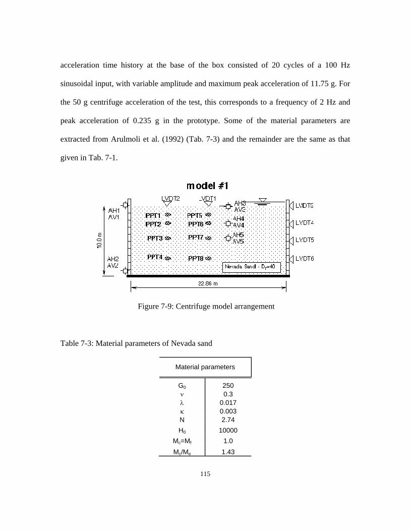
Table 7-3: Material parameters of Nevada sand ..............................................................110
x
LIST OF FIGURES Page
Figure 2-1: Schematic diagram of flow liquefaction ........................................................9
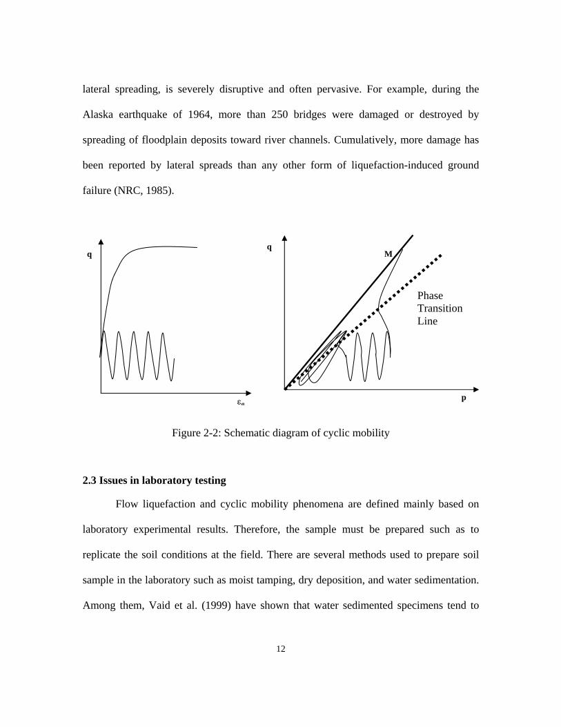
Figure 2-2: Schematic diagram of cyclic mobility ...........................................................11
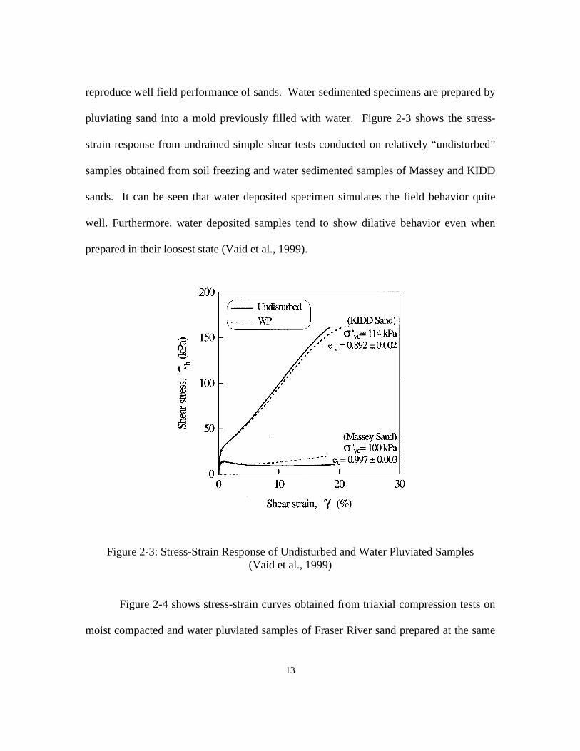
Figure 2-3: Stress-Strain Response of Undisturbed and Water Pluviated Samples (Vaid et al., 1999) .........................................................................................12
Figure 2-4: Influence of Sample Preparation Method on Soil Behavior (Vaid et al., 1999) ..........................................................................................13
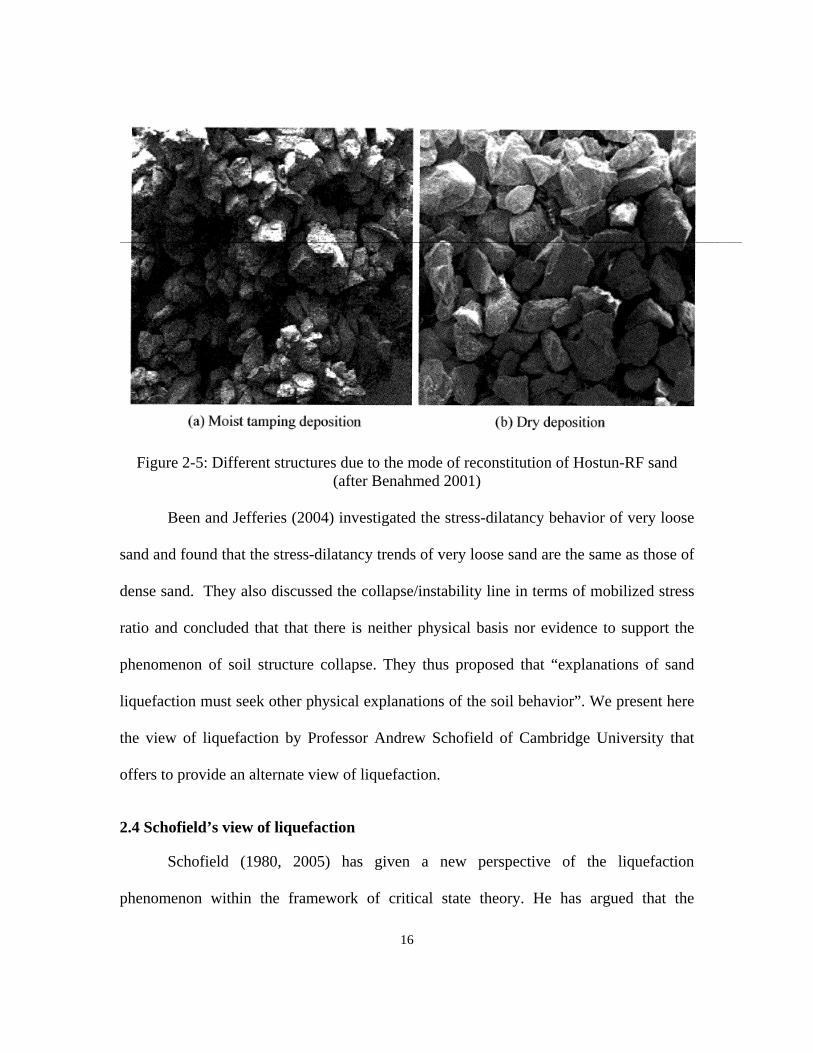
Figure 2-5: Different structures due to the mode of reconstitution of Hostun-RF sand (after Benahmed 2001) .....................................................14
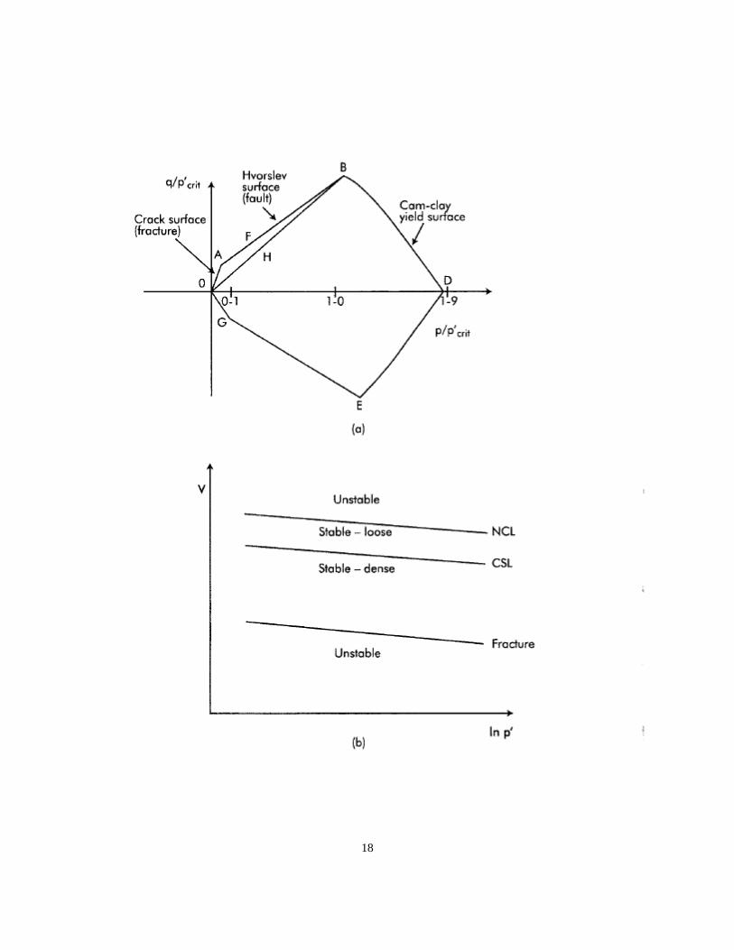
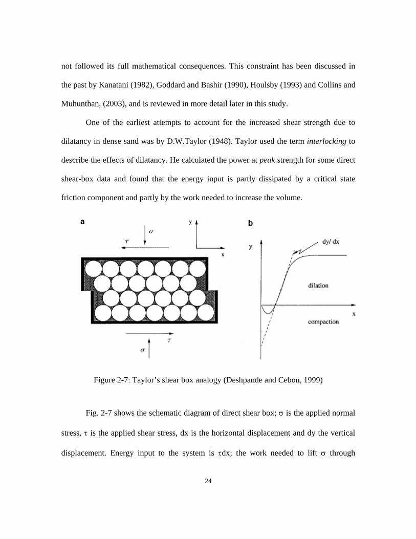
Figure 2-6:Schematic of limits of stable states of soils (a) normalized q/pcrit –p/pcritstress space (b) v- lnp space (Pillai and Muhunthan, 2002)...17 Figure 2-7: Taylor’s shear box analogy (Deshpande and Cebon, 1999) ..........................23
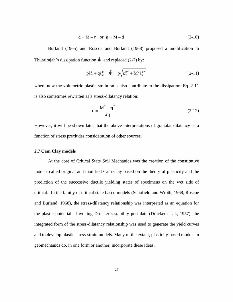
Figure 2-8: Normalized OCC and MCC yield curves ......................................................27
Figure 3-1: The coordinate system used in the void fabric tensor analysis .....................40
Figure 3-2: Schematic description of volume changes in void and solid skeleton..........42
Figure 3-3: Yield locus of new anisotropic sand model with different α values.............48
Figure 3-4: Features of new anisotropic sand model .......................................................51
Figure 3-5: Dilatancy datum in compressive and extensive sides ...................................52
Figure 4-1: Grain Size Distribution for Ottawa F-35 Sand and Glass Beads ..................54
Figure 4-2: Typical drained test results on Ottawa sand..................................................56
Figure 4-3: Variation of ςm with shear strain ...................................................................57
Figure 4-4: The relocation of the CSL as a function of the anisotropy parameter A ......59
Figure 4-5: Variation of maximum anisotropy with vk....................................................62
Figure 5-1: Schematic illustration of the bounding surface in a general stress space .....73
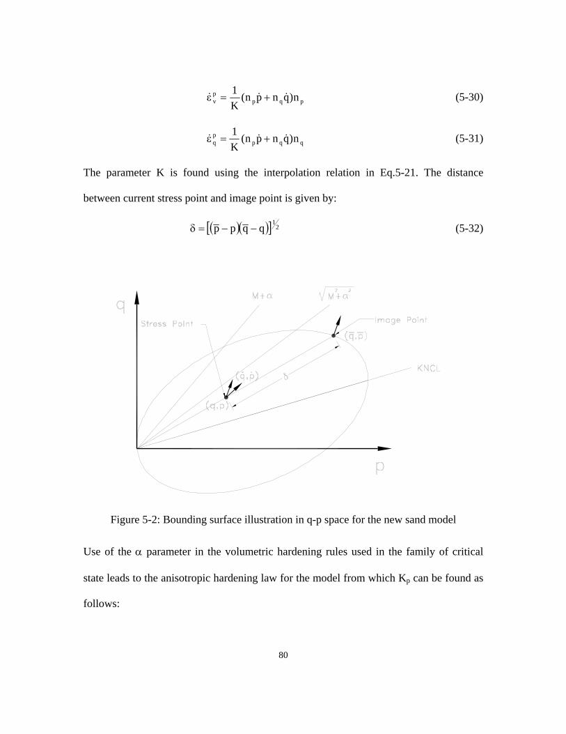
Figure 5-2: Bounding surface illustration in q-p space for the new sand model .............76
xi
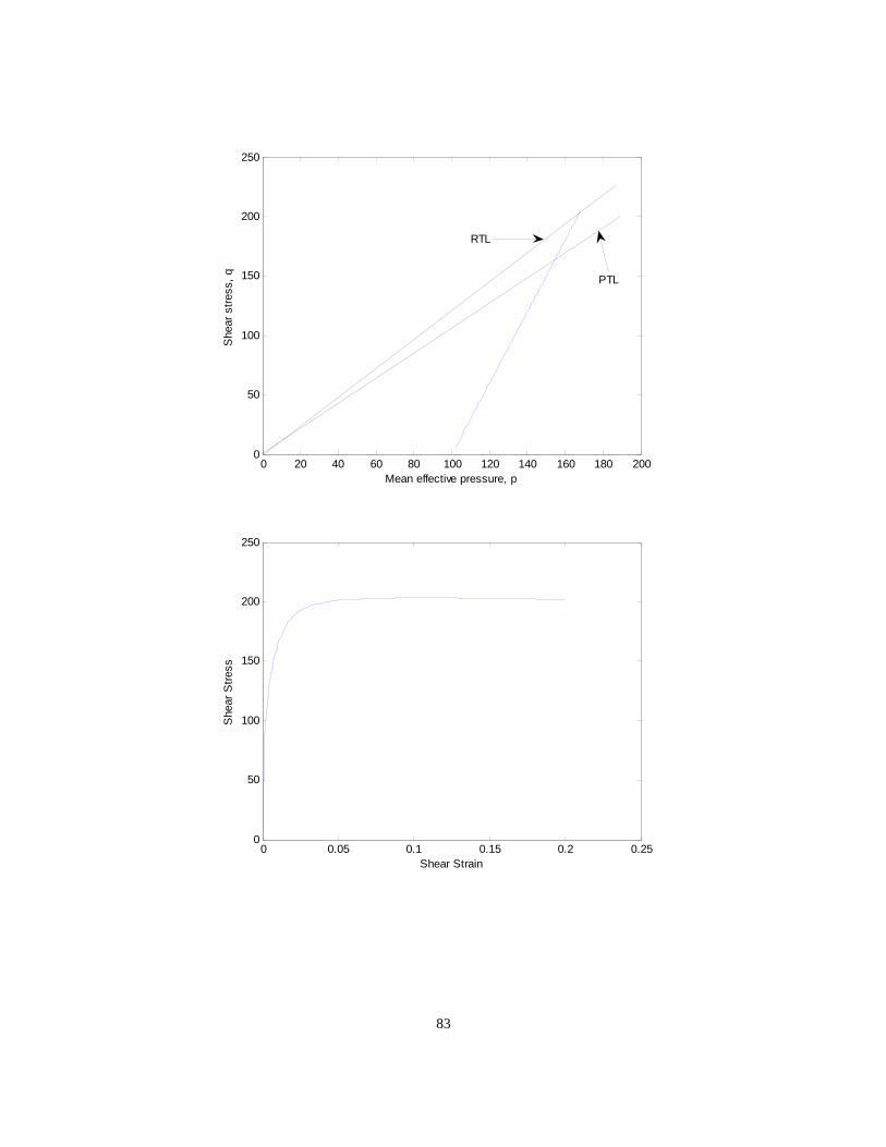
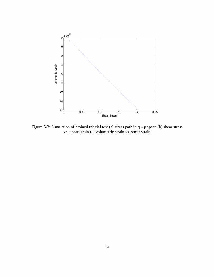
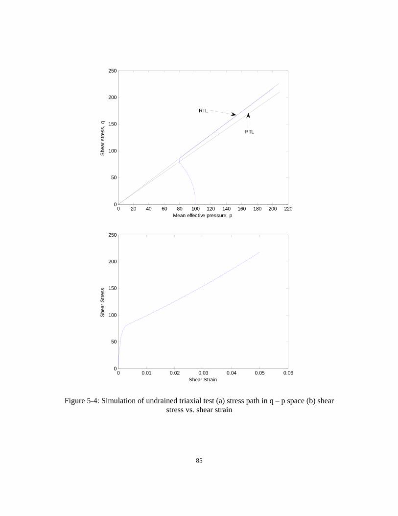
Figure 5-3: Simulation of drained triaxial test (a) stress path in q – p space (b) shear stress vs. shear strain (c) volumetric strain vs. shear strain ..........................79 Figure 5-4: Simulation of undrained triaxial test (a) stress path in q – p space (b)
shear stress vs. shear strain ...........................................................................80
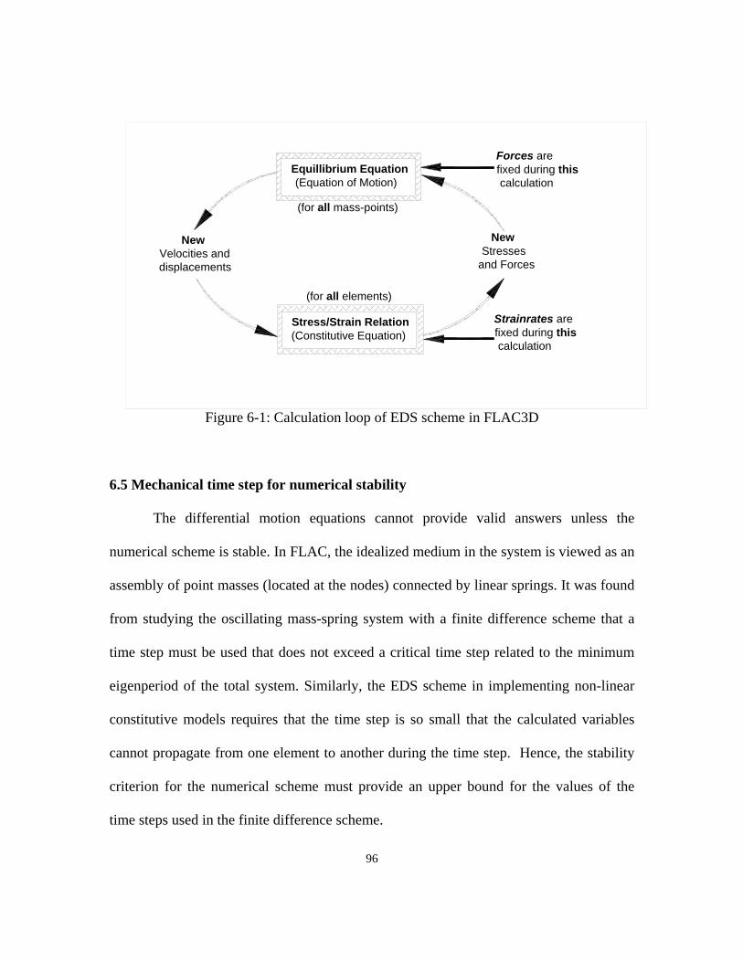
Figure 6-1: Calculation loop of EDS scheme in FLAC3D..............................................54
Figure 6-2: Deformation model for which mixed discretization would be
most efficient ................................................................................................95
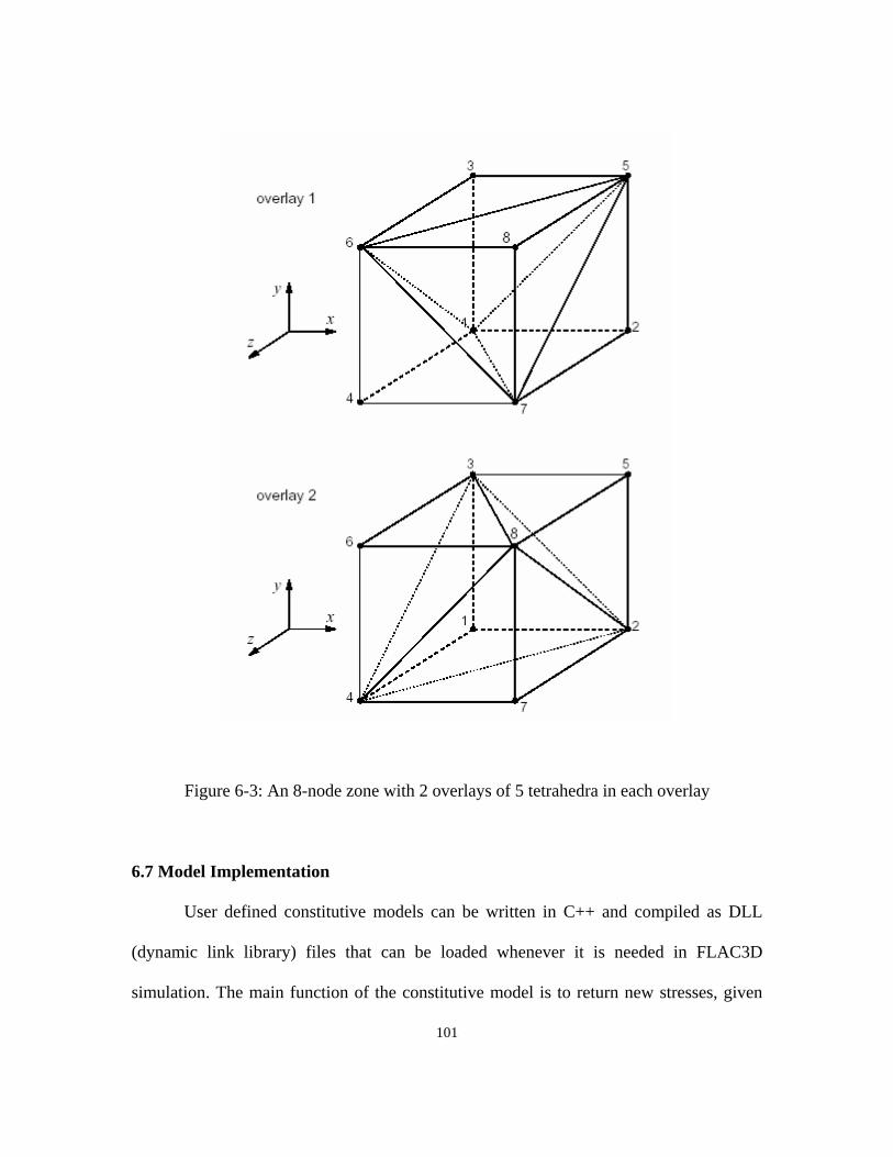
Figure 6-3: An 8-node zone with 2 overlays of 5 tetrahedra in each overlay..................96
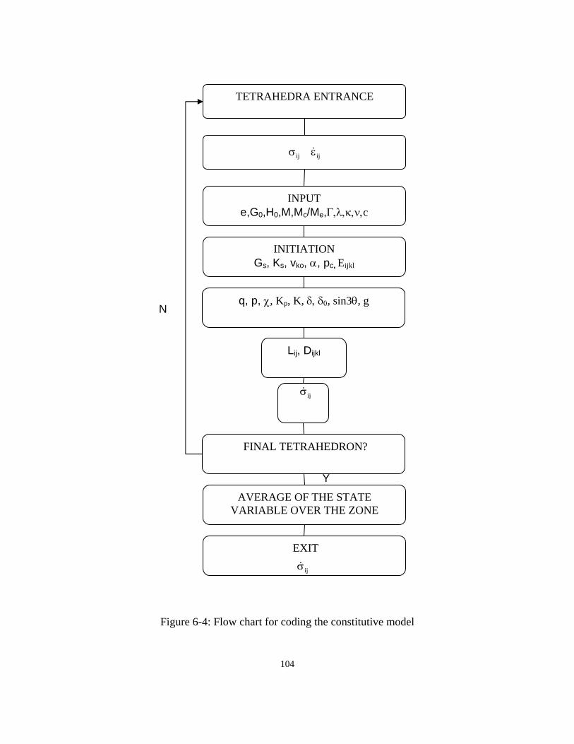
Figure 6-4: Flow chart for coding the constitutive model ...............................................99
Figure 7-1: FLAC3D single zone; boundary conditions..................................................101
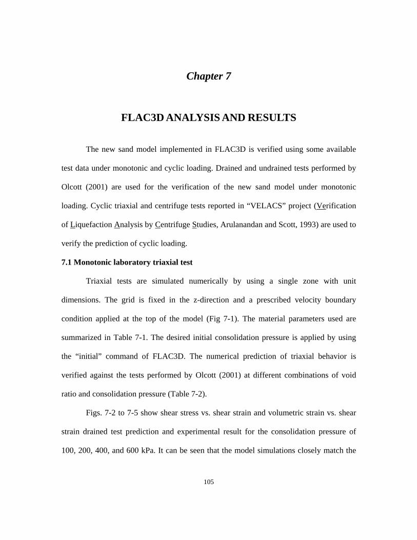
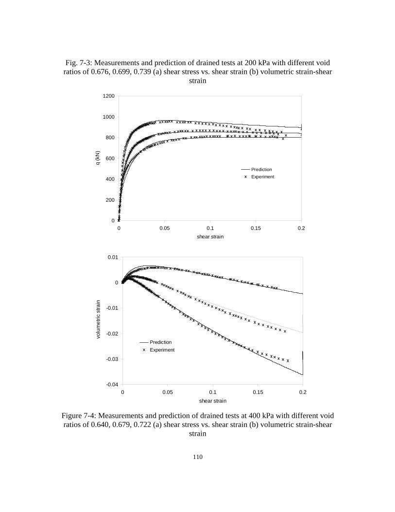
Figure 7-2: Measurements and prediction of drained tests at 100 kPa with different void ratios of 0.637, 0.681, 0.715 (a) shear stress vs. shear strain (b) volumetric strain-shear strain ..................................................................103 Figure 7-3: Measurements and prediction of drained tests at 200 kPa with different void ratios of 0.676, 0.699, 0.739 (a) shear stress vs. shear strain (b) volumetric strain-shear strain ..................................................................104 Figure 7-4: Measurements and prediction of drained tests at 400 kPa with different void ratios of 0.640, 0.679, 0.722 (a) shear stress vs. shear strain (b) volumetric strain-shear strain ..................................................................105 Figure 7-5: Measurements and prediction of drained tests at 600 kPa with different void ratios of 0.670, 0.699, 0.731 (a) shear stress vs. shear strain (b) volumetric strain-shear strain ...................................................................106 Figure 7-6: Measurements and prediction of drained tests at void ratio of 0.640 with different mean effective pressures of 100, 400, 750 kPa (a) shear stress vs. shear strain (b) shear stress vs. mean effective pressure .107 Figure 7-7: Measurement of cyclic triaxial test on Nevada sand consolidated at 80 kPa and void ratio of 0.65 ........................................................................108 Figure 7-8: Prediction of cyclic triaxial test on Nevada sand consolidated at 80 kPa and void ratio of 0.65 ........................................................................108
xii
Figure 7-9: Centrifuge model arrangement......................................................................110
Figure 7-10: FLAC3D model of centrifuge testing .........................................................112
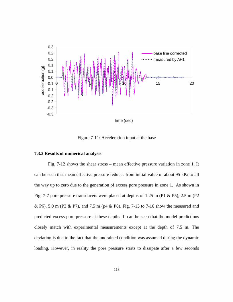
Figure 7-11: Acceleration input at the base .....................................................................113
Figure 7-12: Shear stress – mean effective pressure variation in zone 1.........................114
Figure 7-13: Experimental and prediction of pore pressure of transducer P1 .................114
Figure 7-14: Experimental and prediction of pore pressure of transducer P2 .................115
Figure 7-15: Experimental and prediction of pore pressure of transducer P3 .................115
Figure 7-16: Experimental and prediction of pore pressure of transducer P4 .................116
Figure 7-17: Experimental and prediction of acceleration of accelerometer AH3..........117
Figure 7-18: Experimental and prediction of acceleration of accelerometer AH4..........117
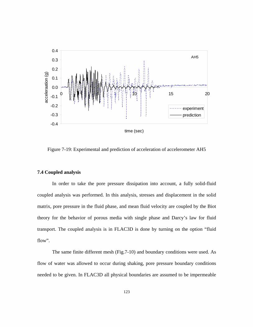
Figure 7-19: Experimental and prediction of acceleration of accelerometer AH5..........118
Figure 7-20: Shear stress – mean effective pressure variation in zone 1.........................119
Figure 7-21: Experimental and prediction of pore pressure of transducer P1 .................120
Figure 7-22: Experimental and prediction of pore pressure of transducer P2 .................120
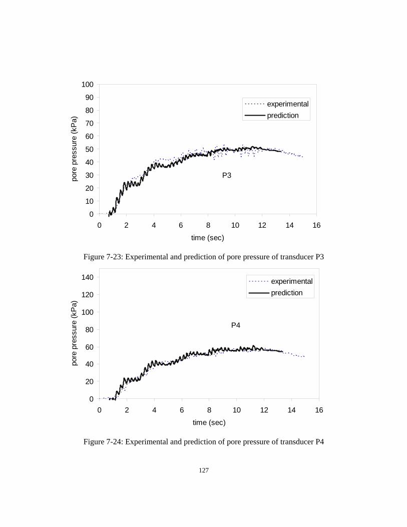
Figure 7-23: Experimental and prediction of pore pressure of transducer P3 .................121
Figure 7-24: Experimental and prediction of pore pressure of transducer P4 .................121
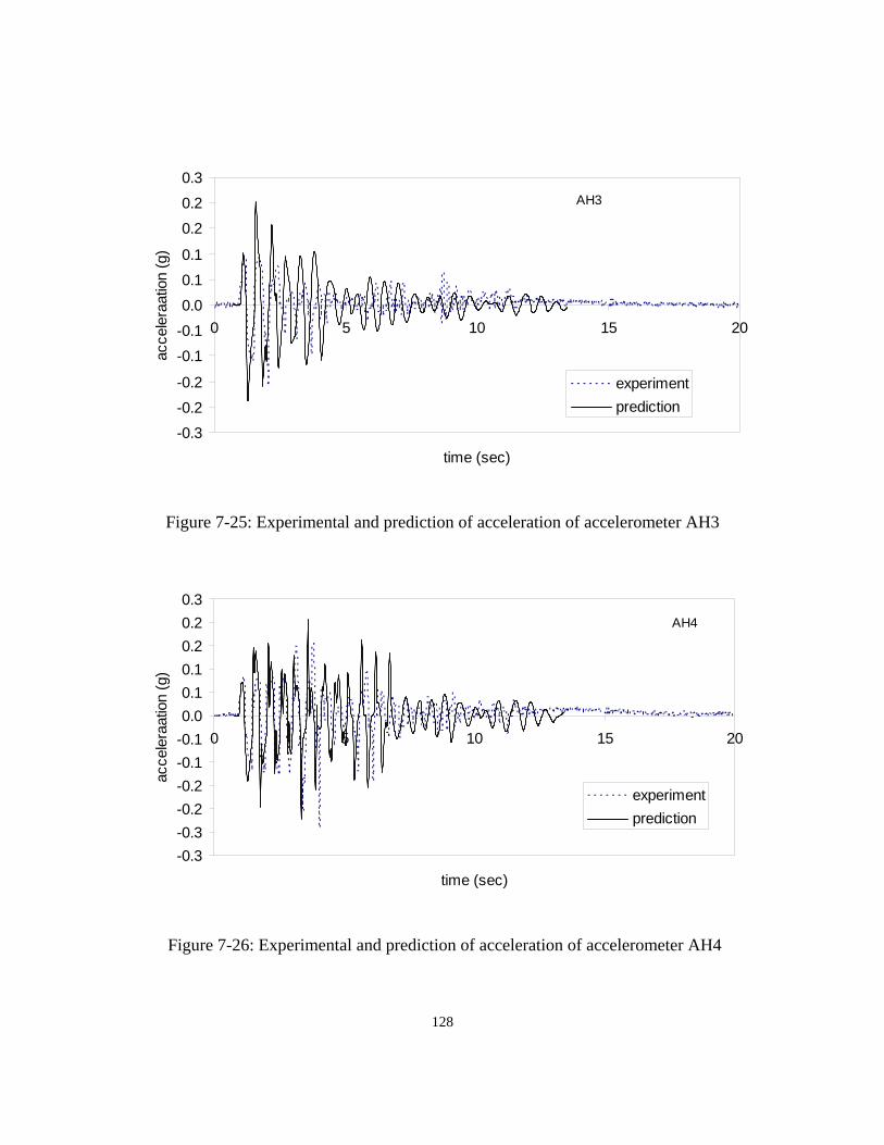
Figure 7-25: Experimental and prediction of acceleration of accelerometer AH3..........122
Figure 7-26: Experimental and prediction of acceleration of accelerometer AH4..........122
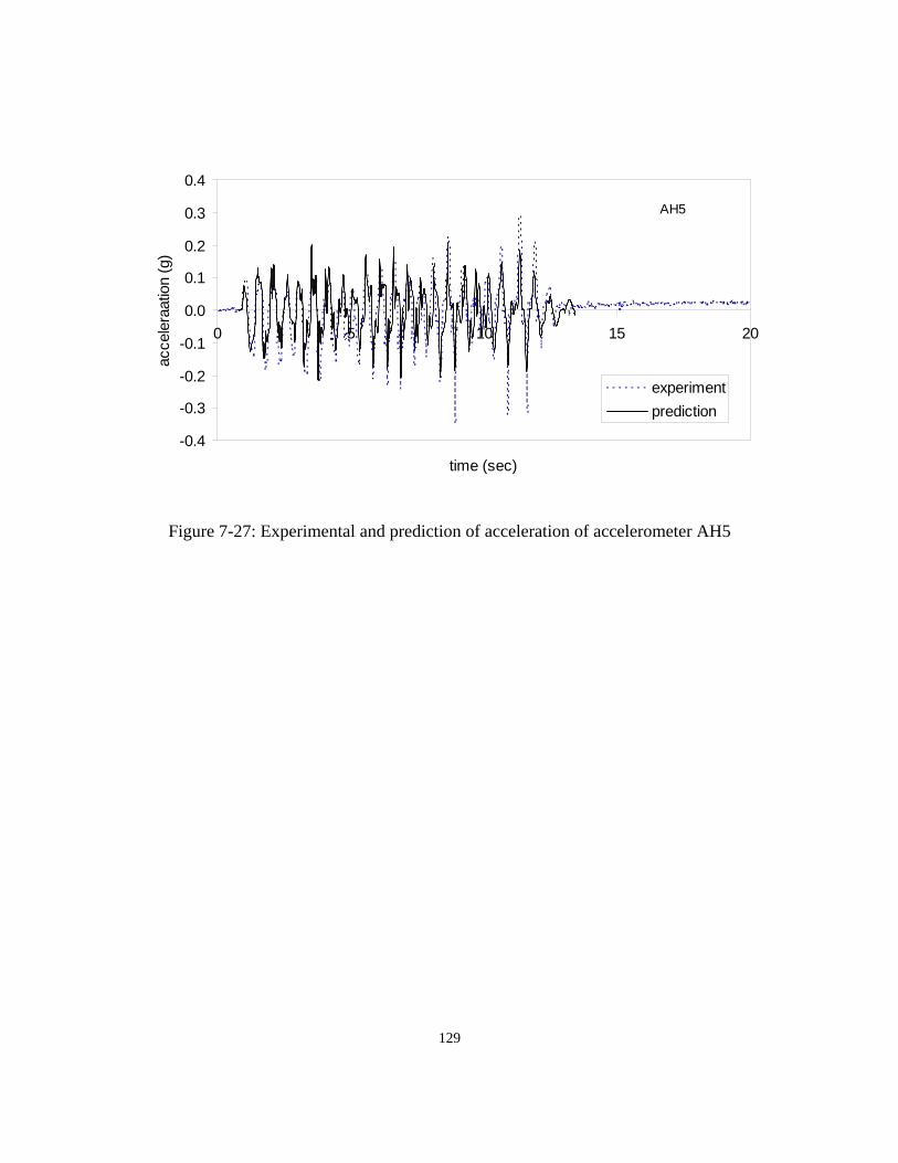
Figure 7-27: Experimental and prediction of acceleration of accelerometer AH5..........123
xiii
Chapter 1
INTRODUCTION
1.1 General
The cost of remediation of liquefaction damages caused by recent earthquakes
often ran into several billions of dollars. This emphasizes the need for the development
of better deterministic tools to predict soil liquefaction and assess post-liquefaction
stability of structures founded on liquefiable soils.
Liquefaction study has been directed mainly towards three different areas after the
two devastating 1964 earthquakes in Niigata in Japan and the Great Alaska earthquake:
field observations during and following earthquakes, laboratory experiments, and
theoretical studies. Lack of instrumentation on most liquefaction failures observed in the
field has made it impossible to obtain recordings of pore pressures and acceleration that
induced liquefaction. Therefore, the investigation of liquefaction phenomena has often
consisted of laboratory experiments and theoretical models. Laboratory experiments
include cyclic triaxial, simple shear, torsional shear testing on samples obtained from the
field by freezing or prepared in the laboratory by different methods. Centrifuge model
testing has also provided a significant input towards developing a better understanding of
liquefaction and related phenomena. Theoretical sand models have also been developed
based on fundamental physics of granular soil behavior and applied to boundary value
1
problems. Realistic constitutive models provide several advantages to liquefaction study.
These include better understanding of soil behavior, extrapolation to conditions that
cannot be produced in laboratory testing and prediction of soil behavior through finite
difference or finite element based numerical techniques so that the liquefaction analysis
can be made on a rational basis.
The critical state framework developed by the Cambridge school in the 1960s has
contributed immensely to the recent developments of comprehensive scientific
approaches to study the shear response of soils. It has also contributed to a fundamental
paradigm shift to soil mechanics and helped bring it properly within the ambit of
continuum mechanics and plasticity theory. Nevertheless, the original critical state
concepts were developed mainly based on the behavior of reconstituted, essentially
isotropic, materials. Therefore, it is well appreciated that, whilst the original Cambridge
critical state models, Cam Clay (Roscoe et al., 1963) and modified Cam Clay (Roscoe
and Burland, 1968) work well for normally consolidated clays, significantly more
complex models are required to capture the essential properties of the mechanics of sands
as well as anisotropically consolidated clays. Recent experimental information has also
shown that the behavior of natural soils, especially sands with pronounced fabric
anisotropy, deviate significantly from the fundamental premises of the critical state soil
mechanics. Moreover, Vaid et al. (1999) have showed that sample preparation methods
(producing different fabric arrangement) greatly influence the stress-strain behavior of
sands.
2
Such deviations have often been attributed qualitatively to the important granular
aggregate fabric which was absent at the outset from the foundations of the original
critical state theory. The absence of the elements of fabric in the fundamental postulates
of the original critical state models has led to many ad hoc proposals relating to critical
state concepts. Non-associated flow rules (Lade and Duncan,1975), some form of shear
hardening (Nova and Wood, 1979), induced anisotropy (Lade,1979), double hardening
concepts (Vermeer,1978), and the improved modeling of dilatancy (Li, 2000), have been
added to the basic structure of critical state theory in order to obtain an acceptable degree
of realism in soil models. Another approach is to introduce fabric related quantities into
the basic structures of critical state soil mechanics. Sand models accounting for fabric
anisotropy not only represent its behavior within the continuum framework, but also give
more physical intuition to the parameters introduced. The present study falls in this
category.
The advances indicated above proved to be successful in modeling the response of
sands under static loads. The sand behavior under undrained cyclic loading, however,
poses additional complexities in numerical modeling. Significant hysteretic behavior
inside the yield surface is a feature of sands under cyclic loading. Moreover, during load
reversal in cyclic load In addition, Bauschinger effect has been observed during load
reversal in cyclic loading experiments. Isotropic hardening models cannot capture such
effects. Moreover, permanent volumetric strains continue to accumulate with each
loading-unloading cycle, which has been shown to be the predominant contributor for the
build up of excess pore pressure that leads to liquefaction. In addition, the mechanical
3
response of solid grains is strongly coupled with the flow of the fluid in the pores of
sands.
Extended plasticity concepts such as multi-surface (Mroz et al., 1981), bounding
surface (Dafalias, 1986), or subloading surface (Hashiguchi, 1989, 1998) plasticity that
were inspired by kinematic hardening laws, have been used to improve the applicability
of monotonic sand models to cyclic loading. These concepts make it easy to account for
the accumulated permanent volumetric strains that occur in sands during cyclic excitation
in a unified manner. In order to relax some of the complexities that arise in the numerical
formulation due to the coupling between two phases it is usually that the assumed
undrained condition prevails during dynamic excitation. However, Seed (1979) reported
that most of the liquefaction failures that occurred some time after the passage of the
main shock were due to the redistribution of excess pore pressure. Thus, the liquefaction
phenomenon is neither fully undrained nor fully drained. Therefore, a fully coupled
formulation based on Biot’s (1941) theory is needed to analyze liquefaction problems.
Recent advances to account for the complexity of sand behavior in cyclic loading
has unfortunately resulted in a rapid increase in model constants where a majority of
them defy physical intuition (Scott, 1988). Thus, more insight is needed into the
controlling features of the mechanical behavior of granular masses (Scott, 1988). This
may only come from a careful interpretation of granular volume changes from a
microscopic point of view.
4
1.2 Objectives of study
This study aims to develop a physically based constitutive model for sand along
the lines of the critical state soil mechanics. It examines the granular volume changes
from a physical and microscopic point of view. It is recognized that plastic volume
changes in sand and granular media, occur due to two reasons: (a) as a result of stress
changes and (b) as a result of changes in fabric during shear deformations (the “Reynolds
Effect”).
The two sources of the plastic volume change in granular media are used to
develop a constitutive model for sand behavior under monotonic and cyclic loading using
bounding surface plasticity theory. The model is subsequently implemented into the
finite difference code FLAC3D and used to analyze liquefaction initiation. FLAC3D is a
widely used commercial 3-dimensional geotechnical software that provides interfaces to
implement user-defined constitutive models. The main objectives of the study are as
follows:
Objective 1: Development of a fabric constitutive model for granular soils
The mechanical behavior of granular media is influenced by their anisotropic
fabric. The directional distribution of porosity in granular media is characterized here by
a functional form. The kinematic relationship between fabric and plastic strain derived
using this form results in the coupling of volumetric strain with shear strain through a
fabric anisotropy parameter. There is also a second volume change in granular media
that occurs as a direct response to changes in stress as in a standard elastic/plastic
5
continuum. This volumetric strain decomposition is used in the Modified Cam Clay
dissipation function and used to develop an anisotropic sand model.
Objective 2: Extension of the model to cyclic loading conditions and application
The new sand is extended to cyclic loading 3-D conditions using bounding
surface plasticity theory (Dafalias, 1986). Emphasis is placed on capturing the hysteretic
behavior of sand and of excess pore pressure build up.
Objective 3: Implementation of the model into numerical codes
The new 3-D sand model is then implemented into FLAC3D. It makes use of
FLAC3D feature that provides a user interface to implement new constitutive models.
External constitutive models can be written in C++ and compiled as DLL (Dynamic Link
Library) files that can be uploaded as needed in a FLAC3D simulation.
Objective 4: Liquefaction analysis
Implemented sand model is used in the liquefaction analysis. A centrifuge test
was simulated and verified with measured test data.
1.3 Organization of the Thesis
Chapter 2 presents a review of the terminologies and the mechanisms that are
currently used to explain liquefaction failures. A brief history of plasticity theory as
applied to soil mechanics is also presented. The chapter highlights the need to better
6
understand granular dilatancy and stress-dilatancy relationships. A review of
modifications made to critical state theory to model sand behavior is also presented.
The representation of fabric and its changes with deformation is presented in
Chapter 3. The developments relating to the decomposition of volumetric strains central
to this study is also provided. Application of this volume decomposition into the
modified Cam Clay dissipation function produces a new anisotropic sand model. The
model produces three important dilatancy datum states. Their importance to sand models
is discussed.
A description of the material parameters used in the soil model and their
determination are provided in Chapter 4. The model parameters are determined using
drained triaxial compression test results. In addition, a function describing the evolution
of the fabric parameter is proposed.
Chapter 5 presents details of the classical plasticity theory and kinematic
hardening laws used. This chapter introduces to the theory of bounding surface plasticity
on which the new anisotropic sand model is formulated for implementation into the
numerical code, FLAC3D. Formulation of the new sand model in q-p space and
generalization of it into six dimensions is also provided.
The implementation of the constitutive model into FLAC3D is detailed in
Chapter 6. The Explicit, Dynamic Solution (EDS) scheme used in Itasca series software
is introduced. Procedures used for dynamic analysis are also provided. The mechanical
time step for numerical stability and mixed discretization technique are presented as well.
7
FLAC3D with the new constitutive model is used in Chapter 7 to simulate
monotonic drained and undrained tests, cyclic triaxial tests, and a centrifuge test
involving liquefaction. Performance of the new sand model is verified against the
measured values.
A summary of the findings of the study as well as some recommendations for
further research are presented in Chapter 8.
8
Chapter 2
BACKGROUND
2.1 Liquefaction
If loose saturated sand is subjected to ground vibration, it tends to compact and
decrease in volume; if drainage is ceased, the tendency to decrease in volume leads to
increase in pore water pressure. If the pore water pressure builds to the point at which it
becomes equal to the overburden pressure, the sand loses its strength completely, and
attains a liquefied state. Although the term liquefaction was first used by Hazen (1920) to
explain the mechanism of flow failure of the hydraulic-filled Calaveras Dam in California
it has now been used to describe a number of different, though related phenomena. The
generation of excess pore water pressure under undrained loading conditions is a
hallmark of all liquefaction phenomena.
The Niigata and Alaskan earthquakes of 1964 triggered the onset of earthquake
induced liquefaction research. The flow slide of the San Fernando earth dam in the 1971
earthquake added further impetus to seismic liquefaction research. The damaging effects
of liquefaction on infrastructure such as roads, buildings, bridges, dams, airports, and port
facilities in the earthquakes of Loma Prieta, California, Kobe, Japan, and most recently in
Sumatra, Indonesia have sustained research efforts in this area.
9
The study of liquefaction has consisted mainly of three different areas: field
observations during and following earthquakes, laboratory experiments, and theoretical
studies. The “critical void ratio” approach suggested by Casagrande (Casagrande, 1936)
is perhaps the first scientific hypothesis to delineate conditions under which liquefaction
might occur. Based on drained shearing tests in which dense sand expanded whereas very
loose sand reduced its volume, he defined the critical void ratio as that at which drained
shear takes place at constant volume. He supposed that liquefaction as the manifestation
of flow failure of sand in states looser than the critical void ratio. The laboratory
experiments of Seed and Lee (1966) showed that even dense sand develops positive pore
water pressure under cyclic loading that leads to liquefaction. Increased laboratory
experimentation and field observation since then has brought forth a number of
liquefaction related terminologies. Flow liquefaction and cyclic mobility are the most
commonly used among these terms to describe the excessive deformation that ensues as a
result of the development of excess pore water pressure.
2.2 Flow liquefaction and cyclic mobility
The typical behavior of saturated loose soils under both monotonic and cyclic
undrained shear tests in laboratory experiments is depicted in Fig. (2-1). Loose soil tends
to compact when sheared and, without drainage, pore water pressure increases. Shear
stress increases monotonically to “peak” stress before it softens and reaches steady state
strength. The points at which the softening occurs fall on a straight line called
“instability” line (Lade and Pradel, 1990; Ishihara, 1993; Chu and Leong, 2002) or
10
sometimes the “Collapse” line (Sladen et al 1985). It was proposed that when the stress
path reaches the instability line, the soil structure collapses leading to development of
high pore pressures. This collapse phenomenon was hypothesized as the main reason for
Vermeer (1978) used a functional form for the shear yield surface to get the first
component of plastic strain. The yield surface closely matched the experimental shear
yield surface by Stroud (1971) and Tatsuoka and Ishihara (1974) and a non-associated
flow rule that is based upon Rowe’s stress-dilatancy relation. The second component of
plastic strain is purely volumetric and a volumetric yield locus is used. Molenkamp
(1981) has produced a far more sophisticated version of Vermeer’s model, with full 3D
capability and consistent derivations, known as MONOT. Ghaboussi and Momen (1979,
36
1982) also used the double hardening principles to construct an elastoplastic constitutive
model for sands which can be used for monotonic as well as cyclic loading conditions.
2.8.5 Stored plastic work
Recently, applications of the thermomechanics framework to geomechanics
problems (Collins and Houlsby, 1997, Collins and Kelly, 2002 and Collins and
Muhunthan, 2003) have had a fair amount of success. It has been shown that the soil
models based on thermomechanics functions, such as the Helmholtz free energy,
dissipation function, do not violate thermodynamic laws as opposed to the plasticity
models derived based on extant procedures. It has been shown that the well-known
original Cam Clay violates thermodynamic laws (Collins and Hilder, 2002; Collins and
Kelly, 2002; Collins and Muhunthan, 2003). The concept of stored plastic work or frozen
energy is the most important aspect of these models. Critical state based soil models often
assume that the energy input to the system is entirely dissipated in frictional work.
Nevertheless, some part of the input energy could be stored within plastically stressed
force chains because of the highly heterogeneous nature of the stress and deformation
fields at the micro level (Collins 2005, Collins and Kelly 2002, Collins and Muhunthan,
2003). The stored energy is represented by the free energy function; the dissipation
function gives the frictional work loss in the system. Once these functions have been
specified, by using a systematic approach, the flow rule, yield condition can be deduced
from them (Collins and Kelly, 2002).
Collins and Houslby (1997) demonstrated that a non-associated flow rule is a
necessary property of a frictional material, in which the plastic deformations are
37
governed by stress ratios rather than by the magnitudes of certain yield stresses as in
metal plasticity. Collins (2005) clarified that there are two causes of dilatation in a soil,
one due to Reynolds dilatancy, the other due to the recovery of the frozen energy. Collins
et al. (2006) have further extended this work and modeled the Reynolds dilatancy in the
framework of thermomechanics.
The original critical state concepts were developed mainly based on the behavior
of reconstituted, essentially isotropic, materials. The behavior of sands, particularly the
angular sands commonly encountered in the field have a better defined granular structure.
These materials possess a significant degree of fabric anisotropy leading to the
difficulties faced by the original critical state models to sands. Yet, none of the sand
models discussed above directly accounted for this phenomenon. As a result while ad
hoc improvements have been made in the predictions by these models, some of the
parameters used by them have little physical meaning.
This study makes use of the fabric based plasticity model for anisotropic behavior
of clays developed by Muhunthan and his colleagues (Muhunthan et al., 1996; Masad et
al., 1998) to develop a physically based model for sands as shown in the next chapter.
38
Chapter 3
THE NEW ANISOTROPIC SAND MODEL
3.1 General
There have been two major trends in describing the soil behavior. The first one is
motivated by plasticity in which a soil medium is treated as a homogeneous continuum. It
provides for a viable means of modeling the behavior of the soil mass (Schofield and
Wroth, 1968). Many useful theories including the critical state soil mechanics framework
have been developed based on this idealization (Roscoe et al, 1963; Roscoe and Burland,
1965).
The second approach is based on micromechanics in which soils are treated as
assemblies of discrete particles. The early stages of this approach treated a soil medium
as an assembly of regular and irregular arrays of rigid frictional particles and derived
analytical solutions to describe their collective behavior (Mindlin, 1949; Rowe, 1962).
The contact distribution of particles in the basic models was subsequently modified with
a probabilistic distribution function to reflect their anisotropic nature (Horne, 1965; Oda,
1972; Matsuoka, 1974). The advances in computational power enabled the simulation of
contact deformation of spheres under loads using Newtonian laws of motion and led to
the development of Discrete Element Method (Cundall and Strack 1978). It has since
become a tool simulate the behavior of an assembly of spherical particles in a computer
39
and has been used to identify a number of problems in granular mechanics including
dilatancy and the development of shear bands (Suiker and Fleck, 2004, Barthust and
Rothenburg, 1990).
The continuum plasticity models often do not account directly for the
micromechanics of granular irreversible deformation whereas the detailed study of the
particulate nature of soil material is mathematically complicated and its applicability to
field problems and design is limited (Scott, 1987).
Therefore, a new approach in which the plasticity theory is improved with the
proper choice of additional parameters based on micromechanics has been used by a
number of researchers. This approach takes advantage of the continuum theory as a
powerful technique for practical applications; however, it recognizes the particulate
nature of soils and incorporates into plasticity theory the features of the spatial
arrangement of solid particles and associated voids, termed granular fabric.
3.2 Fabric measure based on void space
The mechanical behavior of granular materials is strongly influenced by its
microstructure. In triaxial compression tests on sands, Oda (1972b) observed that the
strength of granular soils is different depending on the direction of compression with
respect to the horizontal. Moreover, he observed that non-spherical particles tend to be
rotated perpendicular to the direction of a maximum compression. Void ratio or the
porosity is often used to characterize the state of packing in granular materials. These scalar
measures, however, are insufficient to characterize the directional behavior of granular
40
materials. Higher order micro-structural variables known as “fabric tensors” have been
used to describe the distribution and orientation of grains and voids (Oda et al., 1982,
1985; Mehrabadi et al., 1982; Tobita, 1989; Pietruszczak and Krucinski, 1989a; Bathurst
and Rothenburg, 1990; Muhunthan et al., 1996). Models incorporating fabric measures
are also extant in the literature (Wan and Guo, 2004, Tsutsumi and Hashiguchi, 2005; and
Zhu et al., 2006).
This study makes use of the void fabric tensor measure to characterize fabric effects
in granular media (Muhunthan et al, 1996; Masad and Muhunthan, 2000). Void fabric
tensor is developed based on the concept of a representative elemental volume (REV) which
consists of sufficient number of particles to make the statistical treatment valid. The REV
can be generally of any shape such as cubical, spherical, etc. In this study, an idealized
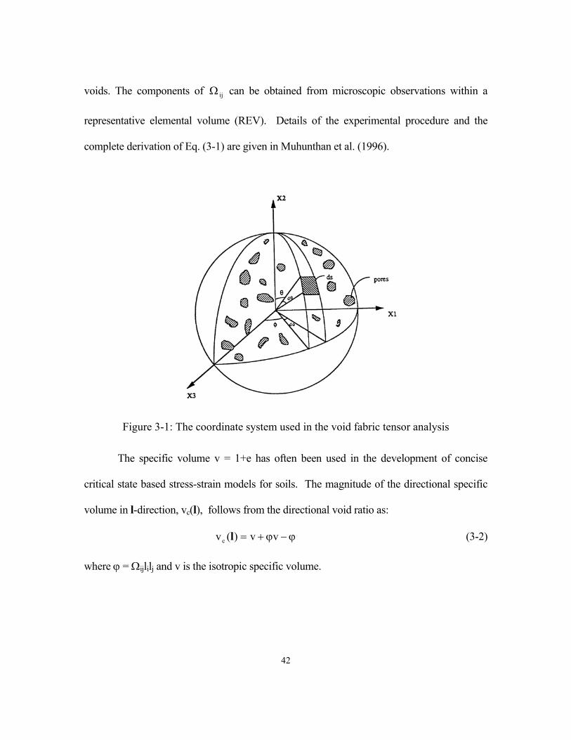
spherical REV with voids shaded as shown in Fig. 3-1 is chosen. Using averaging
techniques the distribution of void ratio within the REV can be approximated by a
directional function ec(l) of the form (Muhunthan et al., 1996; Masad et al. 1998):
( ) ( )jiijc ll1ee Ω+=l (3-1)
where ec(l) is the magnitude of the void ratio vector in the direction of the unit vector l, e is
the isotropic void ratio of the soil, the components of the unit vector l are given by l1 =
sinθsinφ, l2 = cosθ and l3 = sinθcosφ (Fig. 3-1), and Ω ij is termed the void fabric tensor. If
the voids are isotropically distributed, the components of the void fabric tensor become zero
and Eq. (3-1) reduces to the isotropic average value, e, of the void ratio. Thus, the
components of the void fabric tensor represent deviations from the isotropic distribution of
41
voids. The components of can be obtained from microscopic observations within a
representative elemental volume (REV). Details of the experimental procedure and the
complete derivation of Eq. (3-1) are given in Muhunthan et al. (1996).
Ω ij
Figure 3-1: The coordinate system used in the void fabric tensor analysis
The specific volume v = 1+e has often been used in the development of concise
critical state based stress-strain models for soils. The magnitude of the directional specific
volume in l-direction, vc(l), follows from the directional void ratio as:
ϕ−ϕ+= vv)(vc l (3-2)
where ϕ = Ωijlilj and v is the isotropic specific volume.
42
3.3 Fabric change due to deformation
The changes in material points in granular materials induced by deformation are
registered by the evolution of its fabric. Past investigators have explored the relationship
between fabric and strain originating with the seminal contribution by Philofsky and Finn
(1967) who introduced the idea of measuring strain by stereological principles. Kanatani
(1984) extended this work and developed relationships between strain and different fabric
tensors. Satake (1989) developed the average strain in granular materials as a function of the
relative displacement between particles and the branch vector which connects the centroids
of pairs of particles. This is utilized by Iai (1993) to develop a concept of effective strain in
granular materials and re-interpret the stress dilatancy relation in the Cam Clay model (Iai,
1994). In what follows, we explore a simpler relationship between volumetric strain and
changes in void fabric tensor (see also Muhunthan et al. 1996).
The rate of change of volume in granular materials equals the rate of change in
volume of voids, thus the rate of change in void ratio. Differentiating Eq.(3-1):
( ) ( ) jiijjiijc llell1ee Ω+Ω+= &&& l
(3-3)
Summation of the directional rate of volume change over all directions leads to:
(3-4)
jiijc lleee Ω+= &&&
Denoting , Eq. (3-4) can be simplified to: jiij llΩ=ϑ &&
ϑ+= &&& eeec (3-5)
43
The above relationship shows that the rate of change of directional volume consists of two
components; the standard macroscopic component and one that is dependent on the rate of
change of fabric. The decomposition of the rate of volume change is shown schematically as
in Fig. 3-2. In extant granular models, rate of volume change is assumed to occur entirely
within the void skeleton due to contraction/dilation of voids (Fig. 3-2(b)). The derivation
here shows that the evolution of anisotropic granular fabric contributes an additional
contribution to the rate of volume change (Fig. 3-2c). This additional rate of volume change
that occurs within the sample must, therefore, be incorporated in plasticity models to reflect
its contribution.
ėc
Current Practice
Void
skeleton
Solid
skeleton
Void skeleton
Solid
skeleton
Void skeleton
Solid
skeleton
ė
ėi
Present Study
Soil Sample
Figure 3-2: Schematic description of volume changes in void and solid skeleton
For small strains, the rate of volumetric strain in granular materials is equal to the
rate of change of the volume divided by the current total volume (total volume = 1+e).
Dividing Eq. (3-5) by the total volume:
e1e
e1e
e1ec
+ϑ
++
=+
&&& (3-6)
44
Defining e1
ecvc +
=ε&
& and e1
ev +
=ε&
& , Eq. (3-6) can be re-written as;
ϑ+
−ε=ε &&&e1
evcv (3-7)
vε& can be recognized as the standard macroscopic volumetric strain rate measured by
experiments..
Since the fabric tensor Ωij is deviatoric, it is possible to relate its change to the
deviatoric or shear strain change, ijε& through the use of an isotropic tensor valued functional
representation (Boehler, 1987):
( )e,, klklijij εΩΩ=Ω &&& (3-8)
The functional form is generally complex. However, if the principal axes of and are
assumed to be coincident, the relation can be modeled as (Muhunthan et al., 1996):
ijε& ijΩ&
ijij εβ=Ω && (3-9)
with:
( ) ( ) kiik21 e/11ae/11a ΩΩ−+−=β (3-10)
where a1 and a2 are scalar functions of the isotropic void ratio. It is noted in passing that the
detailed relationship between fabric and the strain deviator tensor has been studied by
Kanatani (1985). Denoting qjiij ll ε=ε && for triaxial condition, and multiplying Eq. (3-9) by li
and lj one will get:
qεβ=ϑ && (3-11)
45
where l is chosen at any convenient direction to study fabric changes with deformation.
Substituting Eq. (3-11) in Eq. (3-7) results in:
qvcv e1e
εβ+
−ε=ε &&& (3-12)
The last expression shows that the rate of volumetric strain in is coupled with the rate of
shear strain in anisotropic soils. The relationship Eq. (3-12) can be simplified with the use
of a coupling parameter, as (see also Muhunthan et al. 1996): α
qvvc εα+ε=ε &&& (3-13)
where β+
=αe1
e
It is evident from the above discussion that the relationship between volumetric strain and
shear strain is purely kinematic and is induced by fabric anisotropy.
3.4 Decomposition of plastic strain
Most plasticity models of granular media consider the plastic volumetric strain to be
solely contributed by changes in stress. This precludes contributions from other
mechanisms to plastic volumetric strain. The kinematic relationship between volumetric
strain and fabric relationship developed here enables us to put forward a proposal for an
additional source of plastic strain that arises purely as a result of changes in fabric.
Accordingly, the plastic volumetric strain is considered to be: pvε&
pq
pvc
pv εα−ε=ε &&& (3-14)
Re arranging Eq. (3-14) and denoting pq
pvi εα−=ε &&
46
(3-15) pvi
pvc
pv ε+ε=ε &&&
where is that part that is caused by changes in stress and is that part that arises as
a result of changes fabric anisotropy.
pvcε& p
viε&
The above formulation suggests that the overall plastic volumetric strain rate in
granular materials is contributed by two sources. is that part that arises as a result of
changes fabric anisotropy and thus termed “fabric induced volumetric strain”.
Since , it always remains dilative during loading. This part of plastic
volumetric strain is predominant in granular materials as their aggregate arrangements are
highly anisotropic. The coupling between volume and shape changes observed
qualitatively and termed granular dilatancy by Osborne Reynolds (Reynolds, 1885) has
influenced many a concept in the modeling of the stress-strain behavior of soils.
However, whilst various attempts have been made to incorporate dilatancy into
constitutive models, little regard is made to its mechanical origins. Goddard and Bashir
(1990) have shown that Reynold’s dilatancy is essentially a kinematical constraint.
Further, Kanatani (1982), Goddard & Bashir (1990) and Houlsby (1993) have argued that
such an internal kinematic constraint does not contribute to plastic energy dissipation.
Since is a kinematic constraint and is always dilative, it is assumed here is that
due to Reynolds effect.
pviε&
pq
pvi εα−=ε &&
pviε& p
viε&
Micro-mechanical studies have shown that when a granular material is subjected
to loading, the load is carried by a combination of strong and weak networks ((Radjai et
al). These studies also show that no plastic strains occur in the force chains and all the
47
plastic deformation occurs in the weak frail network. Thus, all plastic energy dissipation
will occur in the weak networks and therefore corresponding strains must be used in the
description of the dissipation function as well as in hardening rules. Based on this
analogy, , the effective plastic volumetric strain is considered to be occurring inside
the weak networks and therefore must be included in both dissipation and hardening
rules.
pvcε&
Division of volumetric strain as in Eq. (3-15) has been explored in the past by
Shamoto et al. (1998) and Zhang et al. (1999) for modeling the behavior of sands under
cyclic loading. A rather different division of the plastic volume strain has been proposed
by Chandler (1985) and Nixon and Chandler (1999). The shear induced plastic strain
is that part of the volume strain which is recovered after a loading cycle; whilst the stress
induced part is the “settlement or accumulated plastic strain” which remains after a
loading cycle is completed. The two volume strains and can hence be thought of
as the “reversible” and “irreversible” plastic volume strains in this context.
Pviε&
Pviε& P
vcε&
According to the proposed division of volumetric strains, both dilative and
contractive volumetric strains are present right from the beginning of loading contrary to
extant constitutive models. The new separation of volume changes in granular media is
incorporated into the plasticity theory to develop a new anisotropic sand model.
48
3.5 Yield loci of anisotropic sand
The proposed division of plastic volumetric strain by the two sources; fabric
induced kinematic , and stress induced enables us to revise the plastic dissipation
function(Eq (9)) proposed by Burland (1965) that was used to develop the modified Cam
Clay model. Kanatani (1982), Goddard & Bashir (1990) and Houlsby (1993) have argued
that since the fabric induced volumetric strain, is the manifestation of internal
kinematic constraints, it does not contribute to plastic dissipation (see also Collins and
Muhunthan 2003; Collins et al. 2006). Thus, we revise Eq. (2-11) as:
Pviε& P
vcε&
Pviε&
2pq
22pvc Mpˆ ε+ε=Φ && (3-16)
Note that only enters into the above dissipation function. We also note that the choice
of the modified Cam Clay dissipation function for revision was motivated by
experimental observations, since, is the compressive “accumulated strain increment”
induced by cyclic loading under drained conditions as discussed in the previous section.
These increments have been found to be approximately normal to a modified Cam Clay
type surface by Chang and Whitman (1988) and Nieumunis et al. (2005). Following the
family of critical state models, equating the revised dissipation function to the plastic
work done results in:
Pvcε&
Pvcε&
( ) 2pq
22pq
pv
pq
pv Mpqp ε+εα+ε=ε+ε &&&&& (3-17)
The above equation can be simplified to give the ratio of plastic strains as:
49
( )α−ηη−α+
=εε
2M 222
pq
pv
&
& (3-18)
Eq. 3-18 can be interpreted as a stress-dilatancy rule, which contains an additional
parameter, the fabric anisotropy α.
Recognizing the plastic strain ratio above as the associated flow rule of the theory
of plasticity, (3-18) can be integrated to give the yield locus for the anisotropic sand
model as (Wood, 1990):
( ) ⎥⎦
⎤⎢⎣
⎡
α−η+= 22
2
c MM
pp (3-19)
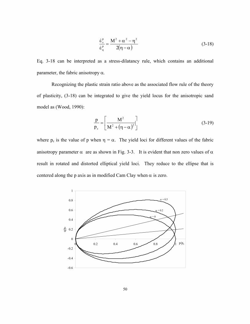
where pc is the value of p when η = α. The yield loci for different values of the fabric
anisotropy parameter α are as shown in Fig. 3-3. It is evident that non zero values of α
result in rotated and distorted elliptical yield loci. They reduce to the ellipse that is
centered along the p axis as in modified Cam Clay when α is zero.
-0.6
-0.4
-0.2
0
0.2
0.4
0.6
0.8
1
0 0.2 0.4 0.6 0.8 1 p/pc
q/p c
α = 0.5
α = 0.2
α = 0
50
Figure 3-3: Yield locus of new anisotropic sand model with different α values
Oda (1993) has also produced yield loci which are distorted ellipses with rotation
when he included the fabric tensor as measure of induced anisotropy for granular
materials. He demonstrated that the yield locus of the shape of the distorted ellipse with
rotation fits very well with the experimentally determined yield locus (Yasufuku, 1990)
for anisotropically consolidated sands.
3.6 Datum states of dilatancy
The inclusion of the fabric anisotropy parameter α in the dissipation function and
consequently in the yield curve results in three important datum states as shown in Fig. 3-
4. Firstly, when subjected to isotropic strains, the resulting stress state is not
isotropic but lies upon the “kinematic normal consolidation line” KNCL, with slope
0pq =ε&
α .
In most critical state based models, relationships of the form (3-19) are often
characterized as a form of stress-dilatancy relationship. However, as discussed earlier
granular dilatancy consists of kinematic (Reynolds type) as well as stress-induced
components. Thus the use of stress-dilatancy in relationships of the form (3-19) is not
appropriate for anisotropic soils. It is just a flow rule as used here (see also Collins and
Muhunthan 2003).
There is a second datum state at which the volumetric strain = 0 and where it
changes its sign from positive to negative. The line on which this occurs is often termed
the phase transformation line (PTL) encountered in undrained tests (Ishihara 1978),
Pvε&
51
though Mroz (1998) suggested the term “Zero dilatancy line” since the plastic volumetric
strain rate is zero on this line. From (19), the slope of the PTL can be determined to be
22M α+=η .
The third datum line corresponds to the state defined by . An expression
for can be derived from Eq. (3-19) using the decomposition of the volumetric plastic
strains (Eq. (3-13)) as:
0Pvc =ε&
Pvcε&
( )α−ηα−η−
=εε
2)(M 22
pq
pvc
&
& (3-20)
When : 0Pvc =ε&
α+=η M ; α−=εε
Pq
Pv
&
& (3-21)
This is the classic Taylor (1948) stress-dilatancy relation. Notice, however, that is
non-zero at this state; therefore, dilation is now entirely due to the Reynolds effect. Even
though the sand is dilating, the dissipation is entirely due to shear as at this state the
dissipation function (3-17) reduces to:
Pviε&
pqT Mpˆ ε=Φ & (3-22)
which is the classical Thurairajah (1961) dissipation function that was used in the original
Cam Clay model (Roscoe et al. 1963). Some further properties of this line were discussed
by Collins and Muhunthan (2003) and Collins (2005), who termed it as the “Reynolds-
Taylor Line” (RTL). As the undrained stress path of dense sands becomes asymptotic to
52
this line, it was also termed as the asymptotic line by Gudehus et al. (1976) or the
“ultimate line” by Poorooshasb (1989) in the literature.
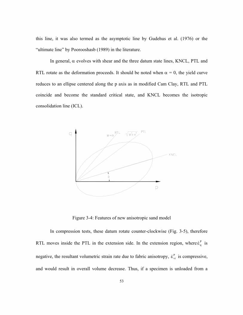
In general, α evolves with shear and the three datum state lines, KNCL, PTL and
RTL rotate as the deformation proceeds. It should be noted when α = 0, the yield curve
reduces to an ellipse centered along the p axis as in modified Cam Clay, RTL and PTL
coincide and become the standard critical state, and KNCL becomes the isotropic
consolidation line (ICL).
Figure 3-4: Features of new anisotropic sand model
In compression tests, these datum rotate counter-clockwise (Fig. 3-5), therefore
RTL moves inside the PTL in the extension side. In the extension region, where is
negative, the resultant volumetric strain rate due to fabric anisotropy, is compressive,
and would result in overall volume decrease. Thus, if a specimen is unloaded from a
Pqε&
Pviε&
53
given dilatational state, at constant pressure, and then sheared in the opposite direction,
the specimen starts to contract plastically, and reach the RTL first with no possibility of
attaining PTL. This would be the case for sands with a collapsible structure for which α
would be negative to begin with.
Usually the shearing in the extensive side develops anisotropy in that direction
destroying the anisotropy that developed in the compressive side. In other words, the
value of the fabric anisotropy parameter goes from positive to negative according to the
sign of plastic shear strain. Upon further deformation the evolution of α and accordingly
the locations of RTL and PTL would essentially follow the pattern as in the case of
normal sands. This has been observed in the past by several experiments on ultra loose
sands (e.g. Alarcon et al. 1988). As one would expect in such a kinematic hardening,
anisotropic model, the material is exhibiting a Bauschinger effect. This is also a feature
of the model of Houlsby (1993), who notes that this is entirely consistent with the
‘sawtooth’ analogy, where there is a definite preferred orientation needed to produce
dilation.
54
Figure 3-5: Dilatancy datum in compressive and extensive sides
The insights gained from the granular dilatancy model and its implications on
plastic dissipation and the yield surface discussed above are utilized in the following
sections to model monotonic and cyclic behavior of sands within the context of bounding
surface elasto-plasticity.
RTL PTL
PTL
RTL
22M α+
22M α+
α+M
α−M
q
p
55
Chapter 4
MODEL PARAMETERS
This chapter presents a discussion of the various parameters of the model and
their determination using laboratory test.
4.1 Experimental observations
A series of drained and undrained triaxial compression tests were conducted by
Olcott (2001) on Ottawa sand, manufactured by U.S. Silica from Ottawa Illinois.
Specimens were prepared using water sedimentation. The sand is a silica sand consisting
of mostly rounded grains with a specific gravity of 2.65. The grain size distribution is
given in Figure 4-1. Soil index properties include a coefficient of uniformity of 1.51,
coefficient of curvature of 0.97, and a mean grain size of 0.44mm. According to USCS,
the sand is classified as poorly graded (SP). The maximum void ratio was determined in
accordance with ASTM D4254-91 Method C. The minimum void ratio was determined
using a slight variation of ASTM D4253-93 (Olcott, 2001). The ASTM maximum and
minimum void ratios for Ottawa F-35 sand were determined to be 0.76 and 0.56
respectively.
56
0
20
40
60
80
100
0.2 0.3 0.4 0.5 0.6 0.7 0.8 0.9 1
Ottawa SandGlass Beads
Perc
ent P
assi
ng (%
)
Grain Size (mm)
Figure 4-1: Grain Size Distribution for Ottawa F-35 Sand and Glass Beads
A Brainard-Kilman Model S-600 triaxial loading frame manufactured by GEO
Store from Stone Mountain, Georgia was used to conduct all triaxial compression tests.
Allowable deformation rates range from 0.0025mm/min to 5.0 mm/min. The maximum
allowable cell pressure for this load frame is 1200 kPa, but limitations such as supply
pressure, maximum line pressures, and regulators limited the maximum allowable cell
pressure to 800 kPa.
Typical measured stress, strain and volume change characteristics of sands with
differing void ratio but consolidated to the same initial confining stress are as shown in
Figure 4-2. It can be seen that the critical state condition is not achieved in any of these
specimens even after 18% of shear strain.
57
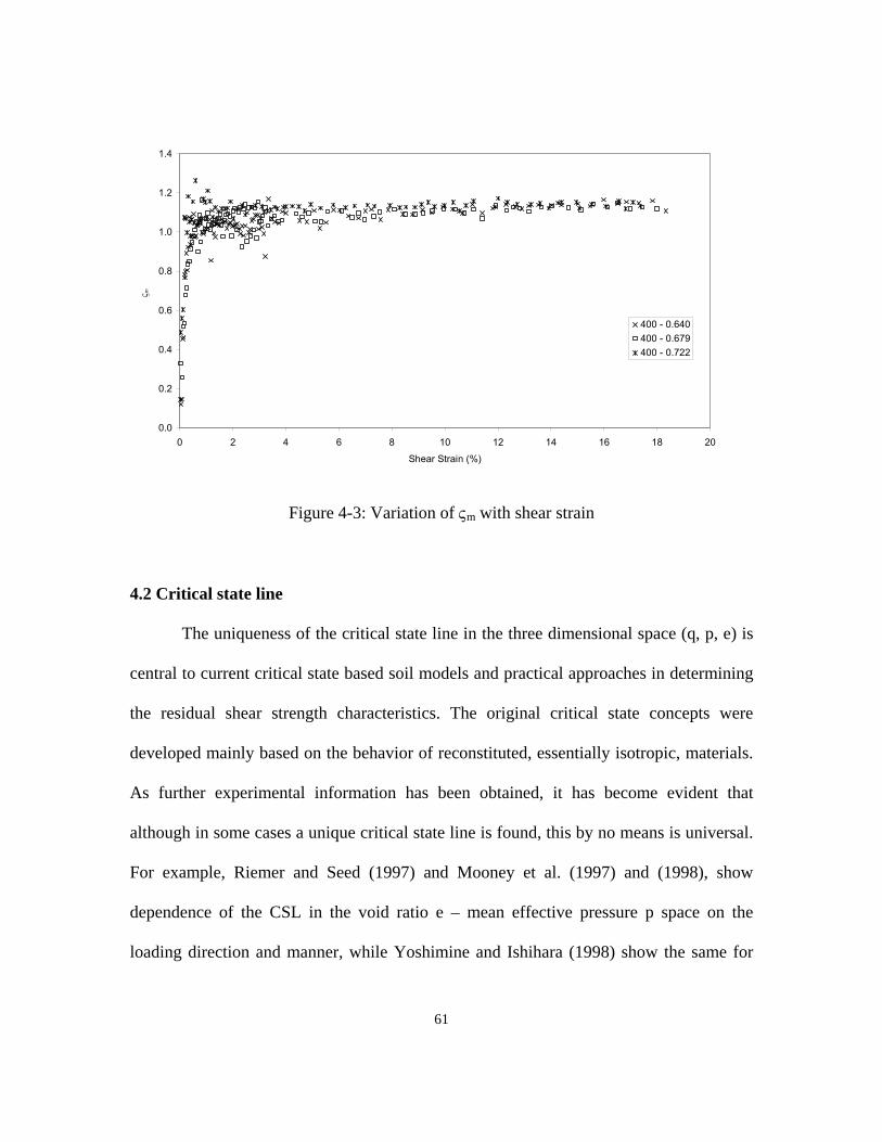
The measured shear stress strain and volumetric values are used to calculate the
plastic dissipation rate,pq
m p
ˆ
εΦ
=ς&
using necessary energy corrections (Muhunthan and
Olcott, 2002; Muhunthan et al. 2004) and plot its variation with strain as shown in Fig. 4-
3. It can be seen that after an initial scatter mς values attain a constant value around 3 to
4 % strain and remains constant beyond. Similar data for simple shear tests have been
given by Stroud – see Muir Wood (1990). As emphasized by Muhunthan et al (2004) this
result enables the slope of the final critical state line in q-p space, to be determined from
data obtained at low strain levels, and so avoiding the difficulties caused by the
development of inhomogeneous deformations, which occur at strains greater than 20%.
Furthermore, the constant value mς is found to be equal to M independent of the
initial consolidated conditions thus reducing the plastic dissipation Φ to Thurairajah’s
dissipation function (Eq. 2-11). Consequently, must necessarily be zero. Thus, in
accord with the proposed theory, the Reynolds Taylor Line (RTL) is attained at this stage
(Eq. 3-20) and sand state continues to remain in this state. Since in this state, the
rate of change of volumetric strain is entirely due to Reynolds dilatancy, given by
(see Eq. 3-14). This is evident from the near linear volumetric response in the
post RTL region for the strains considered here (Fig. 4-2).
TΦ Pvcε&
0pvc =ε&
pq
pvi εα−=ε &&
58
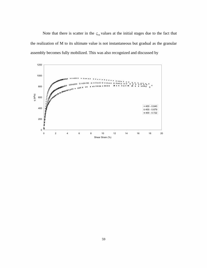
Note that there is scatter in the mς values at the initial stages due to the fact that
the realization of M to its ultimate value is not instantaneous but gradual as the granular
assembly becomes fully mobilized. This was also recognized and discussed by
0
200
400
600
800
1000
1200
0 2 4 6 8 10 12 14 16 18 20
Shear Strain (%)
q (k
Pa)
400 - 0.640400 - 0.679400 - 0.722
59
-0.040
-0.030
-0.020
-0.010
0.000
0.010
0 2 4 6 8 10 12 14 16 18 20Shear Strain (%)
Vol
umet
ric S
train
400 - 0.640400 - 0.679400 - 0.722
Figure 4-2: Typical drained test results on Ottawa sand
Kabilamany and Ishihara (1990). Following their proposal, the variation of M is modeled
by an inverse tangent relation between M and the plastic shear strain:
)S/arctan()MM(MM Pq0f
2o ε−+= π (4-1)
where is the initial value (estimated to be 0.9), and is the final value of M (Fig.4-
2). The value of is 1.14 for Ottawa sand, whilst S is taken to be 0.012.
0M fM
fM
60
0.0
0.2
0.4
0.6
0.8
1.0
1.2
1.4
0 2 4 6 8 10 12 14 16 18 20
Shear Strain (%)
ς m
400 - 0.640400 - 0.679400 - 0.722
Figure 4-3: Variation of ςm with shear strain
4.2 Critical state line
The uniqueness of the critical state line in the three dimensional space (q, p, e) is
central to current critical state based soil models and practical approaches in determining
the residual shear strength characteristics. The original critical state concepts were
developed mainly based on the behavior of reconstituted, essentially isotropic, materials.
As further experimental information has been obtained, it has become evident that
although in some cases a unique critical state line is found, this by no means is universal.
For example, Riemer and Seed (1997) and Mooney et al. (1997) and (1998), show
dependence of the CSL in the void ratio e – mean effective pressure p space on the
loading direction and manner, while Yoshimine and Ishihara (1998) show the same for
61
the ultimate steady state line. The behavior of sands, particularly the angular sands
commonly encountered in the field, appears to deviate significantly from the original
premises of critical state in the sense of a non-unique critical state line. Such deviation
has been attributed to the microstructure or fabric of naturally deposited granular
medium, and sand models accounting for fabric anisotropy have introduced the
possibility of a critical state line in the e – p space which is not unique, but dependent on
the fabric, inherent and/or evolving, with considerable success in simulation of data (Li
and Dafalias, 2002, Dafalias et al., 2004).
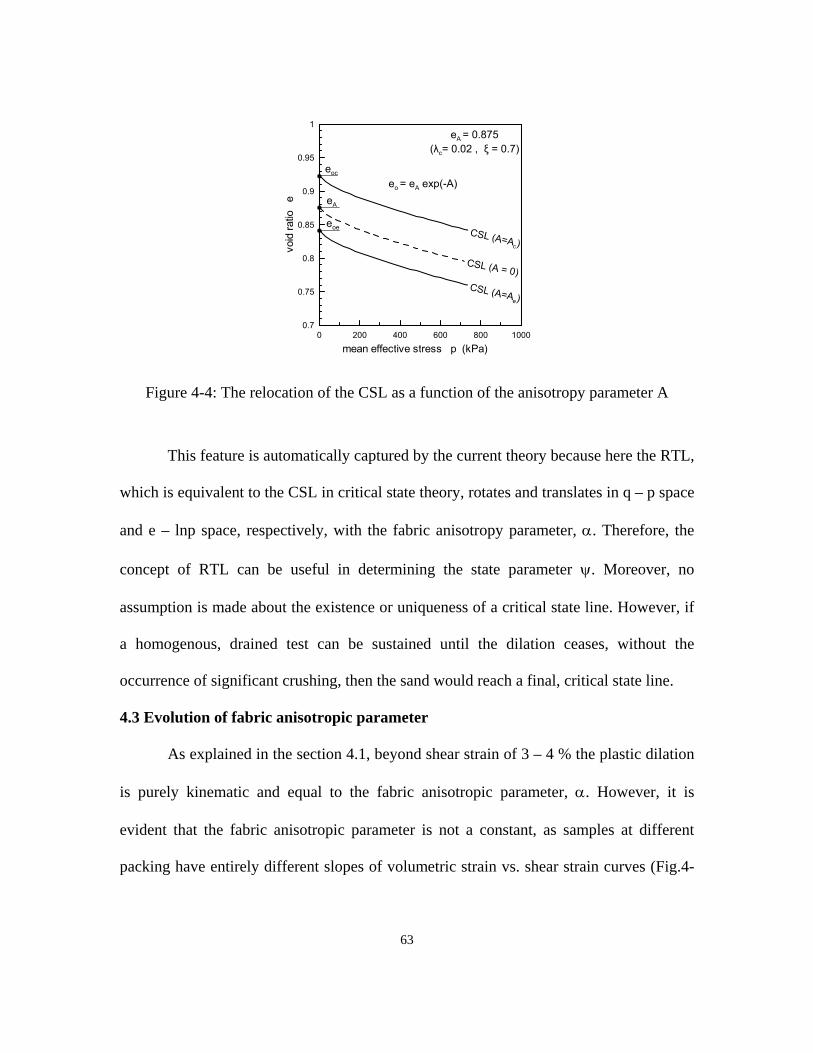
Li and Dafalias (2002) and Dafalias et al. (2004) proposed that the dependence
can be introduced through the value of the critical void ratio e0 at p = 0 as:
)Aexp(ee A0 −= (4-2)
where A is the fabric parameter. The results of this dependence are shown in Fig. 4-4,
where the parallel “translation” of the CSL resulting from such dependence may be
observed. For A = 0 (isotropic fabric) the e0 = eA. Note that Γ≡Ae (Eq. 2-2). Since the
state parameter ψ is now measured from the “translating” CSL, the peak stress ratio Mb
and stress-dilatancy relations are indirectly dependent on the fabric parameter (Sec.2.8.1).
62
0 200 400 600 800 1000
mean effective stress p (kPa)
0.7
0.75
0.8
0.85
0.9
0.95
1
void
ratio
e
CSL (A=Ac)
CSL (A=Ae)
eo = eA exp(-A)
eoe
eA = 0.875(λc= 0.02 , ξ = 0.7)
eA
CSL (A = 0)
eoc
Figure 4-4: The relocation of the CSL as a function of the anisotropy parameter A
This feature is automatically captured by the current theory because here the RTL,
which is equivalent to the CSL in critical state theory, rotates and translates in q – p space
and e – lnp space, respectively, with the fabric anisotropy parameter, α. Therefore, the
concept of RTL can be useful in determining the state parameter ψ. Moreover, no
assumption is made about the existence or uniqueness of a critical state line. However, if
a homogenous, drained test can be sustained until the dilation ceases, without the
occurrence of significant crushing, then the sand would reach a final, critical state line.
4.3 Evolution of fabric anisotropic parameter
As explained in the section 4.1, beyond shear strain of 3 – 4 % the plastic dilation
is purely kinematic and equal to the fabric anisotropic parameter, α. However, it is
evident that the fabric anisotropic parameter is not a constant, as samples at different
packing have entirely different slopes of volumetric strain vs. shear strain curves (Fig.4-
63
2). Desai (1995) has suggested that under a combination of shear and hydrostatic stresses,
anisotropy of geologic materials first increases. But upon further loading, it must
necessarily decrease as the relative magnitude of the hydrostatic stress increases. Thus, as
the loading is increased, the material will self-adjust and tend toward the isotropic state;
which represents an amorphous condition (Drucker, 1991). Horne (1965) had surmised
that during the initial stages of deformation grains tend to align with the major principal
stress direction resulting in the development of anisotropy in that direction. But after
some deformation, when the sliding between particles is no longer confined to specific
directions, the degree of anisotropy decreases, causing a decrease in the stress ratio as
well as the rate of dilation. These proposals suggest that α must vary with shear strain,
beginning at zero, since the material is assumed initially isotropic, here growing to a
maximum level of anisotropy and thereafter reducing progressively. Accordingly, the
following set of equations is proposed to capture the evolution of α:
⎟⎟
⎠
⎞
⎜⎜
⎝
⎛
ε
εα−αε=α
pq
pq
fpqA
&
&&& (4-3)
)vvdexp( 0kk2mf −−α=α (4-4)
where d2 is material constant, αm is the maximum anisotropy that the sample could
develop and ;plnev λ+=κ c00 plnev λ+=κ (e0 is initial void ratio). The Macauley
brackets define the operation Z)Z(hZ = , where h being the Heaviside step function,
which takes zero or one if the argument is less or greater than zero, respectively. The
64
incremental rate of fabric anisotropy parameter has been proposed following Houlsby
(1993).
The rate of dilation with shear strain after attainment of the Reynolds Taylor state
is given by the tangential slope of the volumetric curve (Fig. 4-2 (b), Eq. 3-21). The peak
slope of this curve would correspond to the maximum level of anisotropy, αm, attained.
Using the curves in Fig 4-2(b) and other similar data at various combinations of initial
void ratios and confining pressures (Olcott, 2001), the maximum level of anisotropy αm
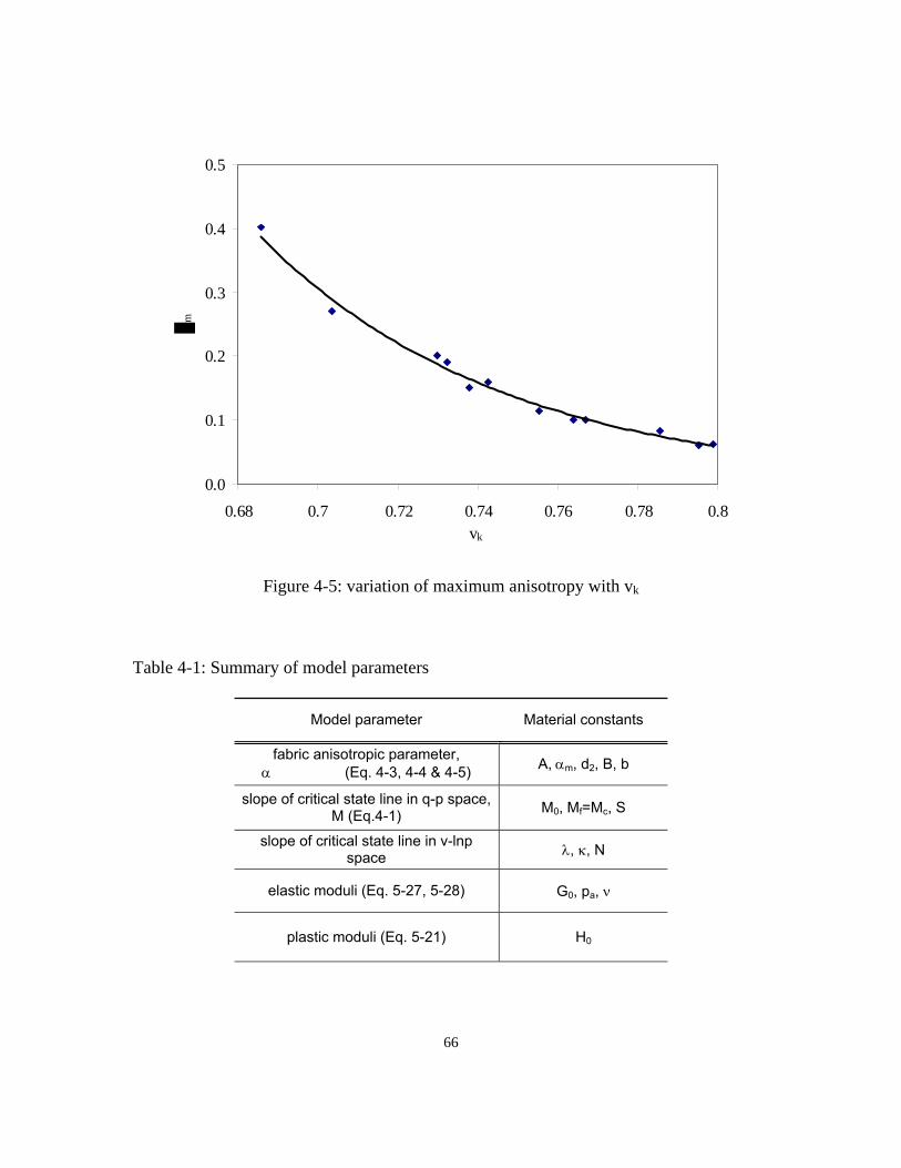
can be calculated and plotted as a function of vk0 as shown in Fig. 4-5. Based on this, αm
is assumed to vary as:
)bvexp(B 0km −=α (4-5)
where and B and b are material constants. For Ottawa sand B = 30405, b =16.44,
respectively.
The following table summarizes the model parameters, the material constants
used in them, and corresponding equations.
65
0.0
0.1
0.2
0.3
0.4
0.5
0.68 0.7 0.72 0.74 0.76 0.78 0.8vk
m
Figure 4-5: variation of maximum anisotropy with vk
Table 4-1: Summary of model parameters
Model parameter Material constants
fabric anisotropic parameter, α (Eq. 4-3, 4-4 & 4-5) A, αm, d2, B, b
slope of critical state line in q-p space, M (Eq.4-1) M0, Mf=Mc, S
slope of critical state line in v-lnp space λ, κ, N
elastic moduli (Eq. 5-27, 5-28) G0, pa, ν
plastic moduli (Eq. 5-21) H0
66
Chapter 5
BOUNDING SURFACE SAND MODEL
5.1 General
The anisotropic sand model developed under triaxial loading in the previous
chapter is extended here to general 3 – D conditions using the bounding surface theory of
plasticity (Dafalias and Popov, 1975). In the early days, the load-deformation problems in
geotechnical analysis were solved by employing the simplest linear elastic or rigid-plastic
material models. However, soil is a multi-phase material that consists of solids, water,
and air; hence its mechanical response is highly nonlinear, inelastic, rate dependent, and
anisotropic. Therefore, in order to describe nonlinear mechanical behavior of soils,
several nonlinear models have been proposed. Nonlinear soil models based on the Mohr-
Coulomb and the hyperbolic stress-strain formulation (Duncan and Chang, 1970) have
been used successfully to model embankments under monotonic loading. Since the
dependence of the stress-strain relationship on stress path and stress history is ignored in
these models the unloading path would trace back the initial loading path unless a
different modulus (unloading-reloading modulus) is used. Masing’s laws (Masing, 1926)
are often used to capture the hysteresis effects of soil response under cyclic loadings.
It is virtually impossible to model path dependence and dilatant characteristics of
soils by elastic models. For example, if a clockwise shear stress produced dilation then
67
conversely an anticlockwise shear stress would have to produce compression (Schofield,
1980). Moreover, granular materials exhibit permanent volumetric deformation during
drained cyclic loading. This permanent volumetric deformation is the primary reason for
the progressive build up of excess pore pressure during undrained cyclic loading that
leads to liquefaction. Several empirical formulations have been proposed to compute the
volumetric strains due to shear strain changes. Martin et al. (1975) proposed an empirical
relationship that relates the incremental volumetric strain, vdε∆ , to the cyclic shear strain
amplitude, , where is presumed to be the “engineering” shear strain and the current
accumulated volumetric strain, :
γ γ
vdε
vd4
2vd3
vd21vd cc
)c(cε+γ
ε+ε−γ=ε∆ (5-1)
where c1, c2, c3,and c4 are constants. It can be noted that the above equation enables the
volumetric strain increment to decrease with accumulation of strains.
An alternative and simpler formula is proposed by Byrne (1991):
)cexp(c vd21
vd
γε
−=γε∆ (5-2)
where c1and c2 are constants which can be related to the relative density, Dr (Byrne,
1991).
Constitutive models that are derived based on plastic theory avoid such empirical
relations because the irrecoverable volume strain is naturally coupled with the shear
strain, and is given by the stress-dilatancy relation. History of the previous loadings can
be tracked by the proper use of plastic internal variables. As strain increment directions
68
are given by the plastic potential function as opposed to the linear elastic theory where
strain increment directions are coaxial to the stress increments, dilative behavior can be
modeled in the theory of plasticity; i.e. both clockwise and anti-clockwise shear would
produce dilation. Thus, the theory of plasticity is central to the advanced developments of
constitutive modeling for liquefaction analysis.
5.2 Classical plasticity
When using the concepts of the theory of classical plasticity, one has to formulate:
(a) the yield condition defining elastic and inelastic deformation domains (b) the flow
rule relating the increments or rates of stress and irreversible strain, and (c) the hardening
rule specifying the evolution of the yield surface in the course of plastic deformation and
the evolution of hardening parameters defining the state of the material. In stress space,
the surface is represented by:
0)q,(F nij =σ′ (5-3)
Since constitutive relations refer to the deformation of the soil skeleton, the state
of the material and yield condition are defined in terms of the effective stress ijσ′ and
plastic internal variables accounting for the past loading history. The internal variables
are usually scalar or second-order tensor quantities such as the plastic work, the plastic
strains, etc.
nq
If small strain theory is assumed, and ijε , , and are total, elastic, and plastic
strains, respectively, the total strain rate is decomposed into:
eijε p
ijε
69
pij
eijij ε+ε=ε &&& (5-4)
The elastic incremental constitutive relations are given by
ijijkleij C σ′=ε && or (5-5) e
ijijklij E ε=σ′ &&
where , are the elastic compliance and moduli matrices, respectively. ijklC ijklE
The plastic constitutive relations require the definition of the direction (or vector)
of plastic loading (flow rule) and the plastic modulus, both functions of the state,
which in turn determine the loading function L as:
ijL
ijijp
LK1L σ′= & (5-6)
where is plastic modulus. Plastic loading, unloading, and neutral loading occur when
L > 0, L< 0, and L = 0, respectively. The inclusion of in L allows for the description
of unstable behavior (softening) when both scalar quantities
pK
pK
ijijL σ′& and are negative
but L > 0 (Dafalias, 1982 & 1986). The plastic strain increment and increment in internal
variables are given in terms of L as:
pK
ijpij RL=ε& (5-7)
nn rLq =& (5-8)
where the brackets define the operation )z(hzz = , h being the Heaviside step
function, and , are functions of the state. In classical plasticity, and are
defined as the gradient of a plastic potential, G = 0, and gradient of a yield locus, F = 0;
ijR nr ijL ijR
70
both are equal to each other if the associated flow rule is assumed, i.e. . is the
direction of the internal variable increment.
FG ≡ nr
The plastic modulus is obtained by the consistency condition: pK
0qqFFF n
nij
ij
=∂∂
+σσ∂∂
= &&& (5-9)
Substituting Eq. 5-8 into 5-9 gives:
nn
p rqFK
∂∂
−= (5-10)
In Cam Clay models, the yield surface is assumed to undergo isotropic and
kinematic hardening along the hydrostatic axis, described by one single scalar , which
measures the plastic volumetric strain. If e is the total void ratio, the plastic volumetric
strain is expressed as
nq
)e1(e
0
ppii +
=ε&
& (5-11)
where is the trace of the plastic volumetric strain rate tensor, epiiε& 0 is the initial void ratio,
and is increment in plastic void ratio. Following the critical state framework, the
plastic void ratio increment, is expressed as:
pe&
pe&
c
cp
pp
)(e&
& κ−λ= (5-12)
Combining (5-11) & (5-12),
71
c
c
0
pii p
p)e1()( &
&+
κ−λ=ε (5-13)
Thus, Kp is given by:
κ−λ+
∂∂
−= c0
cp
p)e1(
pFK (5-14)
Combining (5-4), (5-5), and (5-6), the stress and strain increment for elastoplastic
deformation is expressed as (Dafalias, 1986):
klijklij D ε=σ && (5-15)
where Dijkl, elastoplastic modulus:
klij1
ijklijkl QPB)L(hED −−= (5-16)
rsklrskl LEQ = ; abijabij REP = (5-17)
cdabcdabp RELKB += (5-18)
5.3 Kinematic hardening models
Many of the typical foundation problems encountered by geotechnical engineers
involve stress reversals, rotation of principal stresses and anisotropic behavior.
Earthquake and offshore structures introduce the additional complication of cyclic
loading and degradation.
In the classical theory of plasticity, the region enclosed by the yield surface is
assumed to be purely elastic and plastic deformation is predicted when the stress state lies
on the yield surface and the stress probe is acting outward, i.e. L > 0. Therefore, a loading
that originates from a point inside the yield surface produces elastic deformation until it
72
reaches the yield surface. Thereafter, both plastic and elastic deformations occur during
loading, i.e. L > 0, only elastic deformation is predicted for unloading, i.e. L < 0. On the
contrary, most geological materials such as clay, rock, and sand do not exhibit purely
elastic behavior during unloading and the yield surface, when defined by a small offset
value, usually encloses an elastic domain lying in the vicinity of the loading point.
Indeed, in some cases the yield surface may not exist at all, i.e., most geological materials
experience yield from the very beginning. Moreover, they also show significant
hysteretic behavior during unloading – reloading cycles. Therefore, the isotropic
hardening model cannot reproduce realistic soil behavior as the yield surface expands
uniformly with plastic deformation, so that the size of the elastic region, controlled by the
maximum stresses that have been applied, becomes very large. This feature does not
allow the classical plasticity models to predict strain accumulation in drained and
progressive pore water pressure build up for undrained cyclic deviatoric loading within a
stress domain which has been defined as elastic. Therefore, kinematic hardening models
were proposed to better describe cyclic loading phenomena in soils.
5.3.1 Multi – surface plasticity models
Prager (1955, 1956) was first to introduce the kinematic hardening rule in
plasticity, in which he assumed that yield surface translates without rotation in the stress
space in the direction of the strain increment. Ziegler (1959) modified Prager’s hardening
rule and assumed the rate of translation to take place in the direction of the reduced-stress
vector. In kinematic hardening models, the size of yield surfaces remained unchanged
73
during translation. However, it is argued that mixed hardening rules (Isotropic and
Kinematic hardening) where the yield surface is allowed to translate and expand should
be used for the realistic representation of soil behavior under cyclic loading condition
(Hashiguchi, 1986; Chen and Huang, 1994). Iwan (1967), starting from a one-
dimensional model, generalized for multi-dimensional cases in the stress space by
assuming a collection of yield surfaces arranged in a series-parallel combination instead
of the usual single surface. Each one of the yield surfaces is assumed to obey a linear
work-hardening law of the Prager type, but the combined effect gives rise to a non-linear
hardening law and can effectively model the Bauschinger effect. Independently, Mroz
(1967, 1969) proposed a similar model introducing the concept of the field of work
hardening moduli. This field is defined by a configuration of surfaces of constant work
hardening moduli in the stress space. To do so, he postulated that the response of a
material is governed by a collection of nested yield surfaces, with each surface obeying a
linear kinematic hardening law. He also proposed a new kinematic hardening rule that
controls the movements of the yield surfaces.
As this framework requires many memory surfaces to keep track of previous
loading histories, it is widely called “multi-surface” plasticity. The multisurface
framework has been used by several researchers for both clays and sands under
monotonic as well as cyclic loading conditions (Prevost, 1977, 1985, Elgamal et al.,
2003). Although there are definite advantages in using a multi-surface framework for
modeling soil behavior, it does not have a smooth transition from an elastic to fully
plastic state for reversed loading, which is observed experimentally on most materials.
74
Moreover, in a multi-surface formulation, the plastic modulus varies in piecewise fashion
and this requires large storage capacity in numerical modeling to keep track of the
combined information of many surfaces.
On the contrary, the bounding surface theory of plasticity, originally introduced
by Dafalias and Popov (1976) using the plastic internal variables concept and
independently by Krieg (1975) in conjunction with an enclosed yield surface, uses only
two surfaces; a bounding surface and a loading surface to define a continuous variation of
the plastic modulus between them. Therefore, the bounding surface plasticity formulation
is used in this study. Subloading surface models (Hashiguchi, 1989, 1998) are sub sets of
bounding surface plasticity, as they have the similar structures.
5.4 Bounding surface plasticity
Bounding surface plasticity has been one of the advanced plasticity theories,
which has been applied to numerous problems in geotechnical engineering with a fair
amount of success. The theory assumes that all states of soil behavior are enclosed by a
surface, which was given different names such as limiting (Krieg, 1975), consolidation
(Mroz et al., 1979; Mroz and Norris, 1982), failure (Fardis et al., 1983), or memory
surface (Tseng and Lee, 1983). Dafalias (1986) called this surface the bounding surface,
and in modeling soil behavior, the normal consolidation surface is considered to be the
bounding surface (Dafalias and Hermann 1982; 1986). In spite of the different names, the
role of the enclosed surface is essentially the same, as follows: for any given stress state
within or on the bounding surface, a proper mapping rule associates it to a corresponding
75
“image” stress point on the surface. A measure of the distance between the actual and
image stress points is used in order to specify the plastic modulus at the actual stress state
in terms of a bounding plastic modulus at the “image” stress state (Dafalias, 1986).
Initially the bounding surface theory was applied to clays (Dafalias and
Herrmann, 1986). Bardet (1984, 1986) extended its application to sands using a single
elliptic surface with variable aspect ratio. Crouch et al. (1994) made further advancement
to the bounding surface plasticity for two-dimensional stress space and Crouch and Wolf
(1994 a, b) for three-dimensional stress space. The bounding surface concepts have
become integral to many soil models, especially for the prediction of their cyclic behavior
(Dafalias and Manzari, 1997; Noorzad, 1998; Wang et al., 2002; Li and Dafalias, 2000,
2002). Although the approach is geometric in nature and makes no appeal to physical
reasoning of the problem, it lends itself to a number of general and versatile formulations
in removing the inherent restrictions in the conventional theory of plasticity.
The loading surface or yield surface is assumed to be of the same shape as the
bounding surface (Fig. 4-1). This enables the latter not to intersect but translate and
deform with the bounding surface. The bounding surface and loading surface are defined
by:
0)q,(F nij =σ and 0)q,(f nij =σ (5-19)
respectively, where nq and are internal variables for the bounding and loading
surfaces, respectively.
nq
ijσ is the image point on the bounding surface for the stress
point on the loading surface (Fig.5-1). The image point is found in a way such that the ijσ
76
gradient at the stress point and image point are the same. The plastic modulus on the
loading surface is found using linear interpolation with the distance δ between the image
and stress points. The distance δ is expressed in terms of the coordinates as:
( )( )[ ] 21
ijijijij − σ−σσσ=δ (5-20)
Figure 5-1: Schematic illustration of the bounding surface in a general stress space
The plastic modulus at image point is found using the consistency condition
(Eq. 4-9), and the plastic modulus at the image point, K is given as:
PK
0F =&
ηη−
⎟⎟⎠
⎞⎜⎜⎝
⎛δδ
εσ+= RTL
5.0
0
pijij0P
M),(HKK (5-21)
77
where is the maximum possible distance 0δ δ could take, is a model constant that
depends both on the current stress and accumulated plastic strains, and M
H
RTL is the slope
the RTL. When , ; the loading surface touches the bounding surface and
the standard classical plasticity formulation holds. Inclusion of η into the plastic modulus
allows one to simulate strain softening and control the dilatancy in dense sand. A similar
approach is used by Bardet (1986) and Khalili et al. (2005).
0→δ PKK →
5.5 New sand model in q - p space
The bounding surface version of the new sand model is first formulated in a
triaxial q – p space as there is a vast amount of experimental data available to verify it. It
is then generalized to 3 – D conditions. The bounding surface of the new sand model is
obtained from (Eq. 3-19) as:
( ) 0)pp(pMpqF c22 =−−α−= (5-22)
The loading function L (Eq. 4-6) becomes:
)qnpn(K1L qp && += (5-23)
where
Fp G
pF
n ∂∂
= , F
q Gq
Fn ∂
∂= (5-24)
21
22
F qF
pFG ⎥
⎦
⎤⎢⎣
⎡⎟⎠⎞⎜
⎝⎛
∂∂+⎟
⎠⎞⎜
⎝⎛
∂∂= (5-25)
78
)p2p(M)pq(2pF
c2 −−αα−−=∂
∂ (5-26)
Substituting for using equation (Eq. 5-22), cp
p))(M(p)(2pF 22 α−η−+αα−η−=∂
∂ (5-25)
p)(2qF α−η=∂
∂ (5-26)
5.5.1 Elastic strains
The shear modulus is assumed to be a function of the mean effective pressure, p
and current void ratio e (Richart et al., 1970; Anandarajah, 1994):
21
a
2
a0S pp
e1)e97.2(pGG ⎟⎟
⎠
⎞⎜⎜⎝
⎛+−
= (5-27)
The bulk modulus is related to in terms of the Poisson’s ratio as: SG
)21(3)1(G2KS υ−
υ+= (5-28)
where pa is atmospheric pressure, G0 is the model parameter.
The rate of elastic strains follow as:
S
ev K
p&& =ε ;
S
eq G3
q&& =ε (5-29)
5.5.2 Plastic strains
The bounding surface of the new sand model is as shown in Fig. 5-2. The loading
surface is shrunk to a point (Dafalias and Herrmann 1986). Thus, the image point is now
found using a “radial” mapping and the plastic strains are formulated from (5-7) as:
79
pqppv n)qnpn(
K1
&&& +=ε (5-30)
qqppq n)qnpn(
K1
&&& +=ε (5-31)
The parameter K is found using the interpolation relation in Eq.5-21. The distance
between current stress point and image point is given by:
( )( )[ ] 21
qqpp −−=δ (5-32)
Figure 5-2: Bounding surface illustration in q-p space for the new sand model
Use of the α parameter in the volumetric hardening rules used in the family of critical
state leads to the anisotropic hardening law for the model from which Kp can be found as
follows:
80
κ−λε
=κ−λ
εα+ε=
pvc
c
pq
pv
cc p)(
pp&&&
& (5-33)
pcpvc
c
cp n
ppFK
ε∂∂
∂∂
−= (5-34)
qppc nnn α+= (5-35)
[ ]pG
)(MppMK
F
22c2
pα−η−
κ−λ= (5-36)
5.5.3 Formulation of incremental stress-strain relations
The total volumetric and deviatoric shear strain increments are given as:
pv
evv ε+ε=ε &&& (5-37)
pq
eqq ε+ε=ε &&& (5-38)
Substituting Eq. (5-29), (5-30) and (5-31) into Eq. (5-37) and (5-38), the incremental
stress-strain relation for the triaxial loading condition can be obtained as:
⎟⎟⎠
⎞⎜⎜⎝
⎛⎥⎦
⎤⎢⎣
⎡=⎟⎟
⎠
⎞⎜⎜⎝
⎛εε
qp
CBBA
q
v
&
&
&
& (5-39)
where
ppS
nnK1
K1A += (5-40)
qpnnK1B = (5-41)
81
qqS
nnK1
G31C += (5-42)
For undrained loading, the condition of the total volumetric strain increment is
zero, . 0v =ε&
5.5.4 Model prediction
The above formulation was coded into MATLAB and some simple simulations
were performed to ensure that the new sand model captures the behavior of sand. Typical
predictions of drained and undrained tests by the model are shown in Fig. 5-3 and 5-4.
Both tests start from mean effective pressure of 100 kPa, with the void ratio of 0.72. In
the drained test, the sample initially contracts for stress states below PTL. Once the stress
path crosses the PTL, the behavior changes from contraction to dilation. The sample
continues to dilate at RTL as shown in Fig.5-3 (a) & (c). Similarly, in the undrained test,
positive pore water pressure builds up initially below PTL. Once the stress path crosses
the PTL, it begins to dilate, and negative pore water pressure builds up. In this case also,
the sample continues to dilate at RTL as shown in Fig.5-4 (a). Therefore, the model
predicts the sand behavior satisfactorily in q – p space.
82
0 20 40 60 80 100 120 140 160 180 2000
50
100
150
200
250
Mean effective pressure, p
She
ar s
tress
, qRTL
PTL
0 0.05 0.1 0.15 0.2 0.250
50
100
150
200
250
Shear Strain
She
ar S
tress
83
0 0.05 0.1 0.15 0.2 0.25-14
-12
-10
-8
-6
-4
-2
0
2x 10
-3
Shear Strain
Vol
umet
ric S
train
Figure 5-3: Simulation of drained triaxial test (a) stress path in q – p space (b) shear stress vs. shear strain (c) volumetric strain vs. shear strain
84
0 20 40 60 80 100 120 140 160 180 200 2200
50
100
150
200
250
Mean effective pressure, p
She
ar s
tress
, qRTL
PTL
0 0.01 0.02 0.03 0.04 0.05 0.060
50
100
150
200
250
Shear Strain
She
ar S
tress
Figure 5-4: Simulation of undrained triaxial test (a) stress path in q – p space (b) shear stress vs. shear strain
85
However, it is evident from Fig. 5-5 that the incremental formulation does not
capture the actual behavior of sand during unloading. This has also been the case with
past investigations (Dafalias and Manzari, 2004). Dafalias and Manzari (2004) chose to
modify their stress-dilatancy relation (Eq.12 ) with an ad hoc term to represent the “effect
of fabric” to capture this behavior. We present a new mechanism based on the plastic
volumetric strain decomposition to rectify this defect. It is conceived that the dilatational
volumetric strains are held up by the applied stress ratio and these are “reversible” during
unloading. Subsequently, during unloading as the stress ratio decreases, the dilatational
volumetric strain is recovered. Thus, the reversible plastic volumetric strain takes the
form:
[ ]βη−−=ε e1cpv (5-39)
where c, β are constants, and is the dilatational volumetric strain during the
unloading. Constant c can be found equating with the conditions at the point of load
reversal.
pvε
Eq. (5-39) can be rewritten in rate form by taking derivatives,
ηβ=ε βη− && ecpv (5-40)
The prediction of the proposed mechanism is shown in Fig. 5-5 and it can be seen
that it agrees well with the experimental data.
86
0
200
400
600
800
1000
1200
0 200 400 600 800 1000p
q
without modification
with modification
Fig.5-5: Typical loading-unloading stress path
5.6 Generalization of new sand model
The new anisotropic sand model is now generalized into six dimensional spaces
using invariants in order to implement it into numerical code such as FLAC3D. The
stress invariants and their gradients are defined by (Dafalias and Herrmann, 1986):
iiI σ= ; ijij
Iδ=
σ∂∂ (5-43)
2/1
ijijss21J ⎟
⎠⎞
⎜⎝⎛= ;
J2sJ ij
ij
=σ∂∂ (5-44)
3/1
jikjik sss31S ⎟
⎠⎞
⎜⎝⎛= ;
⎥⎥⎦
⎤
⎢⎢⎣
⎡⎟⎠⎞
⎜⎝⎛=θ −
31
JS
233sin
31 (5-45)
87
⎥⎥⎦
⎤
⎢⎢⎣
⎡δ−⎟
⎠⎞
⎜⎝⎛−
θ=
σ∂θ∂
ijij
3
2kjik
ij 32
J2s
JS3
Jss
3cosJ23 (5-46)
where is the Kronecker delta; θ is the Lode angle which takes the values of for
the loading conditions of triaxial compression and extension. The deviatoric tensor ,
shear stress q, and the mean effective stress p are defined as:
ijδ 6/π±
ijs
ijijij ps δ−σ= ; 3Ip 1= ; J3q ±= (5-47)
Yield function can be written as:
0),,J,I(F =κθ (5-48)
Gradient of the yield function Lij is given as:
⎥⎥⎦
⎤
⎢⎢⎣
⎡δ−⎟
⎠⎞
⎜⎝⎛−
θ++δ= θ
ijij
3
2kjik
ijJ
ijIij 32
J2s
JS3
Jss
J,F
3cos23s
J2,F
,FL (5-49)
The fabric anisotropy parameter α is replaced with a second order dimensionless
deviatoric tensor αij, which is related to α of triaxial space as:
21
jiij23
⎟⎠⎞
⎜⎝⎛ αα=α (5-50)
Rewriting the new sand model (Eq.3-19):
0)pp(pM)ps(:)ps(F c2
ijijijij =−−α−α−= (5-50)
The partial derivative of yield function F with respect to I, J, and M:
3/)p2p(M:)ps(,F c2
ijijij32
I −−αα−−= (5-51)
ijijijJ s
J2)ps(2,F α−= (5-52)
88
)ppp(M2,F 2cM −−= (5-53)
The energy dissipation equations in the family of critical state models have been
formulated as a function of the frictional constant M. However, sand possesses different
critical state strength values for compression and extension. In the triaxial compression
( ) and extension ( ) regions, the energy dissipation must necessarily be
governed by the triaxial compression (M
0q > 0q <
c) and triaxial extension (Me) critical state
parameters, respectively. The parameters Mc and Me can be obtained from the friction
angle using the Mohr-Coulomb failure criterion.
The critical state parameter M is therefore interpolated between Mc and Me as:
)c,(gMM c θ= (5-54)
where θ−−+
=θ3sin)c1(c1
c2)c,(g ; c
e
MM
c =
Partial derivative of M with respect to θ is given as:
θ−−+θ−
=θ
3sin)c1(c13cos)c1(3
M,M (5-55)
The evolution law for α (Eq.4-3 & 4-4) is generalized as:
⎟⎟
⎠
⎞
⎜⎜
⎝
⎛
⎟⎟⎠
⎞⎜⎜⎝
⎛
ε′ε′
ε′α−αε′=α
21):(
signAp
ijp
ij
pij
ijfij
pijij
&&
&&&
where is the deviatoric part of the plastic strain tensor. pijε′&
ij0kk20fij n)vvdexp( −−α=α ;
21)L:L(
Ln
ijij
ijij ′′
′= (5-56)
where is the deviatoric part of the gradient . ijL′ ijL
89
Chapter 6
MODEL IMPLEMENTATION
6.1 General
The Fast Lagrangian Analysis of Continua in 3 Dimensions (FLAC3D) was
developed by Itasca Consulting Group, Inc. as a general three-dimensional procedure for
analysis of geotechnical/geological media subjected to static, dynamic, water flow, and
thermal loading conditions (Itasca, 2002). FLAC3D uses a finite difference approach that
incorporates the Lagrangian description capable of computing large deformations. It has
gained wide acceptance among practicing engineers and researchers as a tool for the
design and analysis of a range of engineering problems in rock mechanics, geomechanics,
and soil mechanics. It has also been successfully used to numerically simulate a number
of geotechnical problems. Besides many built-in nonlinear soil constitutive models such
as Mohr-Coulomb, Cam Clay, etc., it provides a user interface to implement new
constitutive models. FLAC3D is therefore selected for the current study.
6.2 Dynamic analysis
The dynamic analysis option in FLAC3D permits three-dimensional, fully
dynamic analysis with FLAC3D. The calculation is based on the explicit finite difference
scheme to solve the full equations of motion, using lumped grid point masses derived
from the real density of surrounding zone as opposed to fictitious masses used for static
90
solution. FLAC3D also permits analysis of soil-interaction brought about by ground
shaking by coupling the dynamic formulation with the structural element model. The
dynamic option in FLAC3D is applicable to a wide range of problems in disciplines such
as earthquake engineering, seismology, and mine rock burst.
Earthquake loading is basically a cyclic loading because of the shear wave
transmission though the soil layers. “Equivalent-linear” and fully nonlinear methods are
two commonly used in earthquake engineering for analyzing wave transmission and
dynamic soil-structure interaction. In the equivalent-linear method (Seed and Idriss,
1969), a linear analysis is performed, with some initial values assumed for damping ratio
and shear modulus in the various regions of the model. With the reference to laboratory-
derived curves that relate damping ratio and secant modulus to amplitude of cyclic shear
strain, an iterative procedure is performed until there are no further change in assumed
and determined soil properties. In contrast, only one run is done with a fully nonlinear
method, since nonlinearity in the stress-strain law is followed directly by each element as
the solution marches on in time. If appropriate nonlinear laws are used, the dependence of
damping and apparent modulus on strain level is automatically modeled.
Although the equivalent-linear method is conceptually simple and user-friendly, it
takes drastic liberties with physics. On the other hand, the fully nonlinear method
correctly represents the physics but demands more user involvement. If a comprehensive
constitutive model is available, the fully nonlinear method can be used to reproduce some
of the more-subtle dynamic phenomena. FLAC3D uses the latter procedure in solving
dynamic problems. As the new anisotropic sand model captures the nonlinear behavior of
91
sands well, the new sand model is implemented into FLAC3D to simulate the
liquefaction phenomena.
6.3 Modeling dynamic pore pressure generation
Besides modeling the mechanical response of solid materials, FLAC3D also
models the flow of fluid through a permeable solid, such as soils. The flow modeling may
be done by itself, independent of the usual mechanical calculations of FLAC3D, or it may
be done in parallel with the mechanical modeling in order to capture the effects of
fluid/solid interaction (Coupled analysis). Fluid/solid interaction involves two mechanical
effects. First, the fluid in a zone reacts to mechanical volume changes by a change in pore
pressure. Second, changes in pore pressure cause changes in effective stress, which
affects the response of the solids. In FLAC3D by default, the pore fluid simply responds
to changes in pore volume caused the mechanical dynamic loading. The average pore
pressure remains essentially constant in the analysis. However, if the permanent
volumetric strain is accounted properly, FLAC3D generates excess pore pressure
accordingly.
6.4 Explicit, Dynamic Solution (EDS) Scheme
Numerical solution schemes face several difficulties when geomaterial models are
implemented (Hart and Detournay, 2005). Three characteristics of geomaterials cause
specific problems in implementing constitutive models.
1. Physical instability: Physical instability occurs in materials with softening behavior,
such as rock, concrete and dense/over-consolidated soils. The softening behavior
occurs when the material fails and parts of it accelerate and the stored energy is
92
released in the form of kinetic energy. Numerical solution schemes often have
difficulties at this stage because the solution may fail to converge when a physical
instability arises.
2. Path dependence of nonlinear materials: In most geo-mechanical systems, there are an
infinite number of solutions that satisfy the equilibrium, compatibility and
constitutive relations that describe the system. These solutions are corresponding to
different stress paths, respectively. A correct solution needs to be identified for the
actual stress path. For example, if an excavation is made suddenly (e.g., by explosion)
then the solution may be influenced by inertial effects that introduce additional failure
of the material. This may not be seen if the excavation is made gradually. The
numerical solution scheme should be able to accommodate different loading paths in
order to apply the constitutive model properly.
3. Nonlinearity of the stress-strain relation: This is referred to as the dependence of the
elastoplastic stiffness matrix on the stress state. The numerical scheme needs to be
able to accommodate the various forms of nonlinearity.
The above three characteristics of geo-materials, which cause difficulties in
implementing the constitutive model, can all be addressed by using an explicit, dynamic
solution (EDS) scheme, which is used by FLAC3D (Itasca, 2002) to implement elasto-
plastic constitutive models for soils and rocks. The scheme allows the numerical analysis
to follow the evolution of a geologic system in a realistic manner, without concerns about
numerical instability problems. In the explicit, dynamic solution scheme, the full
dynamic equations of motion are included in the formulation, and the static equilibrium
93
state is reached by absorbing the energy in the system through inertial terms added in the
formulation. During the ‘collapse’ failure process in softening materials, some of strain
energy in the system is transferred into kinetic energy. The kinetic energy radiates from
the source and dissipates through the inertial terms in the full dynamic formulations.
Therefore, the numerical solution is always stable even when the system being modeled
is unstable. On the contrary, schemes that do not include inertial terms must use some
numerical procedure to treat physical instabilities. Even if the procedure is successful at
preventing numerical instability, the stress path taken may not be a realistic one.
However, the EDS scheme can follow the physical path and simulate the effect of the
loading path on the constitutive response.
The EDS scheme also allows the implementation of strongly nonlinear
constitutive models because the general calculation sequence allows the field quantities
(velocities/displacements and forces/stresses) at each element in the model to be
physically isolated from one another during one calculation step. This implementation in
the general calculation sequence is described as follows.
The general calculation sequence for the EDS scheme is illustrated in Figure 6.1.
The figure presents the calculation sequence of one loop calculation for one time step and
for each tetrahedron element. In each sequence loop of the time step, the calculation
solves two sets of equations: equilibrium of motion and constitutive relationships. The
former is invoked to derive the new velocities and displacements from stresses and forces
at each mass point. By application of the Gauss divergence theorem to the tetrahedron
element, the derived velocities at each mass point are used to express the strain rates of
94
the tetrahedron element. Then, the constitutive equations are used to calculate new stress
from strain rates. The key feature here is that each box in Fig. 6-1 updates all model
variables from known values that remain fixed while control is within that box. For
example, the lower box takes the set of velocities already calculated and, for each
tetrahedron element, computes new stresses. The velocities and other variables are
assumed to be frozen for the operation of the box, i.e., the newly calculated stresses do
not affect the existing velocities. The assumption is valid provided the time step is so
small that the calculated variables cannot propagate from one element to another during
this time step. This EDS approach makes the implementation of the non-linear
constitutive model possible. All inputs of strain rates and other variables in one
tetrahedron element, during the time step, are fixed and not affected by the calculations in
other elements. The stress increment calculation from strain rate is straightforward and
there is no need to use any iteration process even if the constitutive law is highly
nonlinear.
95
Equillibrium Equation (Equation of Motion)
Stress/Strain Relation (Constitutive Equation)
New Velocities and displacements
New Stresses and Forces
(for all mass-points)
(for all elements)
Strainrates are fixed during this calculation
Forces are fixed during this calculation
Figure 6-1: Calculation loop of EDS scheme in FLAC3D
6.5 Mechanical time step for numerical stability
The differential motion equations cannot provide valid answers unless the
numerical scheme is stable. In FLAC, the idealized medium in the system is viewed as an
assembly of point masses (located at the nodes) connected by linear springs. It was found
from studying the oscillating mass-spring system with a finite difference scheme that a
time step must be used that does not exceed a critical time step related to the minimum
eigenperiod of the total system. Similarly, the EDS scheme in implementing non-linear
constitutive models requires that the time step is so small that the calculated variables
cannot propagate from one element to another during the time step. Hence, the stability
criterion for the numerical scheme must provide an upper bound for the values of the
time steps used in the finite difference scheme.
96
In FLAC3D, a characteristic of the numerical scheme is that a uniform unit time
step is adopted for the whole system. And, the nodal masses in the motion equations
are taken as variables and adjusted to fulfill the local stability conditions.
t∆
The one-dimensional, one series mass-spring system governed by the differential
equation is:
tdxdmkx 2
2
=− (6-1)
where k is the stiffness of the spring, and m is the point mass. The critical time step
corresponding to a second-order finite difference scheme for the equation is given by:
km4t =∆ (6-2)
For an infinite series spring-mass case, the limit-stability criterion has the form
( )2tkm ∆= (6-3)
By selecting , the system will be stable if the magnitude of the point mass is greater
than or equal to the spring stiffness. In FLAC3D, the validity of Equation (6-3) is
extended to one tetrahedron by interpreting m as the nodal mass contribution m
1t =∆
l at local
node l and k as the corresponding nodal stiffness contribution kl. The nodal mass
contribution as derived from the infinite series criterion provides an upper-bound value
for the system under consideration. In order to obtain a stable numerical scheme, the
nodal mass contribution should be given a value that is equal to or larger than the nodal
stiffness contribution. By a simple diagonalization technique of the local stiffness matrix,
the nodal stiffness contribution at local node l is given by
97
[ ]2llq
1qq Sn
V9k α
= (6-4)
where G34K1 +=α , K is the bulk modulus, and G is the shear modulus. No
summation is implied on repeated index q of kqq, which runs from 1 to 3. Then the upper-
bound value for the nodal stiffness contribution can be expressed as:
)k,k,kmax(k 332211l = (6-5)
which yields the expression for the tetrahedron mass contribution at node l:
( ) ( )[ ]( )3,1i,SnmaxV9
m 2lli
1l =α
= (6-6)
to provide a numerically stable solution.
6.6 Mixed discretization
The EDS scheme in FLAC3D is set up on the basis of tetrahedron elements. The
tetrahedron element is a constant strain-rate, three-dimensional element. However, these
elements do not provide for enough modes of deformation when used in the framework
of plasticity. For example, they cannot deform individually without change of volume as
required by certain important constitutive laws and exhibit an over-stiff response as
compared to that expected from the theory. To overcome this problem, a process of
mixed discretization is applied in FLAC3D, as described in Marti and Cundall (1982).
For the mixed discretization technique, more volumetric flexibility is applied to
an element by proper adjustment of the first invariant of the tetrahedral strain-rate tensor.
A coarser discretization in zones is superposed on a finer tetrahedral discretization. Then,
98
the technique is accomplished by assigning the first strain-rate invariant and the first
stress tensor invariant of any particular tetrahedron as the volumetric-average over all
tetrahedral elements in a zone. As shown in Fig. 6-2, the individual tetrahedron will not
keep constant volume when subjected to the pattern of deformation; however the total
volume of the assembly of the tetrahedral elements (i.e. the zone) remains constant under
that deformation pattern.
In FLAC3D, the discretization starts with zones. Then, each zone is internally
discretized into tetrahedral elements. An eight-node zone, for instance, can be discretized
into two different configurations of five tetrahedral elements (corresponding to overlay1
and overlay2 in Fig. 6-3). The calculation of nodal force can be carried out using one
overlay or a combination of two overlays. The advantage of the two-overlay approach is
to ensure symmetric response for symmetric loading.
99
Figure 6-2: Deformation model for which mixed discretization would be most efficient
100
Figure 6-3: An 8-node zone with 2 overlays of 5 tetrahedra in each overlay
.7 Model Implementation
tive models can be written in C++ and compiled as DLL
(dynam
6
User defined constitu
ic link library) files that can be loaded whenever it is needed in FLAC3D
simulation. The main function of the constitutive model is to return new stresses, given
101
strain increments. C++ is an object-oriented computer language using classes to represent
objects. The data associated with an object are encapsulated by the object and are
invisible outside the object. Communication with the object is by member functions that
operate on the encapsulated data. In addition, there is strong support for a hierarchy of
objects. New object types may be derived from a base object and the base-object’s
member functions may be superseded by similar functions provided by the derived
objects. This arrangement confers a distinct benefit in terms of program modularity and
the program can access the derived classes through the base objects.
The emphasis of the object-oriented approach of C++ is to provide a base class
that in
Dim, State *ps)” as a main
interfac
cludes a framework for implementing constitutive models, which are classes
derived from the base class. The base class, called ‘ConstitutiveModel’, is termed an
‘abstract’ class because it declares a number of ‘pure virtual’ member functions. This
means that no object of the base class can be created and that any derived-class object
must supply real member functions to replace each of the pure virtual functions of the
base class. The methodology of writing a constitutive model in C++ for operation in
FLAC3D includes descriptions of the base class, member functions, registration of
models, information passed between the model and FLAC3D, and the model state
indicators. The implementation is achieved by supplying real member functions to
replace each of the pure virtual functions of the base class.
A member function “const char *Run(unsigned u
e is called for each sub-zone (up to ten per zone for a two-overlay case ) at each
cycle from within FLAC3D’s zone scan. The model is coded within the member function
102
and updates the stress tensor from the strain increment tensor for each sub-zone at each
cycle. The structure “ps” contains the current stress components and the computed strain
increment components for the sub-zone being processed. For each sub-zone cycle,
besides the updated stress tensor, the state parameters must also be returned.
As opposed to the implementation of constitutive models based on the
conven
he the anisotropic sand model is shown in Figure
6.4. Th
tional plasticity, the trial-and-correction approach, which is adopted by all built-in
models implemented in the FLAC3D manual, is not used in the implementation of
bounding surface constitutive model. This is because the yielding surface that defines the
pure elastic deformation range doesn’t occur in the bounding surface models. The main
objective of the current model implementation is to calculate the elastoplastic stiffness
matrix ijklD shown in Equation (3-26).
T flow chart for programming
is program is included in the member function “const char *Run(unsigned uDim,
State *ps)”. Each tetrahedral element calls this member function for each cycle to update
the stress state of the tetrahedron. After all tetrahedral elements in the zone are scanned,
the state variables of the zone are modified according to the rule of the mixed
discretization scheme. However, the modification of the stress state of the zone will be
left for FLAC3D. The member function ConfineModulus(void) is used to return a value
for its best estimate of the maximum confined modulus. This is used to determine the
stable time step.
103
TETRAHEDRA ENTRANCE
ijij εσ &
INPUT e,G0,H0,M,Mc/Me,Γ,λ,κ,ν,c
INITIATION Gs, Ks, vko, α, pc, Eijkl
q, p, χ, Kp, K, δ, δ0, sin3θ, g
Figure 6-4: Flow chart for coding the constitutive model
Lij, Dijkl
ijσ&
FINAL TETRAHEDRON?
AVERAGE OF THE STATE VARIABLE OVER THE ZONE
EXIT
ijσ&
N
Y
104
Chapter 7
FLAC3D ANALYSIS AND RESULTS
The new sand model implemented in FLAC3D is verified using some available
test data under monotonic and cyclic loading. Drained and undrained tests performed by
Olcott (2001) are used for the verification of the new sand model under monotonic
loading. Cyclic triaxial and centrifuge tests reported in “VELACS” project (Verification
of Liquefaction Analysis by Centrifuge Studies, Arulanandan and Scott, 1993) are used to
verify the prediction of cyclic loading.
7.1 Monotonic laboratory triaxial test
Triaxial tests are simulated numerically by using a single zone with unit
dimensions. The grid is fixed in the z-direction and a prescribed velocity boundary
condition applied at the top of the model (Fig 7-1). The material parameters used are
summarized in Table 7-1. The desired initial consolidation pressure is applied by using
the “initial” command of FLAC3D. The numerical prediction of triaxial behavior is
verified against the tests performed by Olcott (2001) at different combinations of void
ratio and consolidation pressure (Table 7-2).
Figs. 7-2 to 7-5 show shear stress vs. shear strain and volumetric strain vs. shear
strain drained test prediction and experimental result for the consolidation pressure of
100, 200, 400, and 600 kPa. It can be seen that the model simulations closely match the
105
experimental results. Fig. 7-6 shows the prediction and experimental results for the
undrained tests performed at the void ratio of 0.64 and mean effective pressures of 100,
400, and 750 kPa. Model predictions have again good agreement with experimental
results.
Prescribed velocity
Confining stress
Figure 7-1: FLAC3D single zone; boundary conditions
106
Table 7-1: Material parameters of Ottawa sand
Material parameters
G0 125 ν 0.3 λ 0.016 κ 0.005 N 2.74 H0 10000
Mc=Mf 1.14 Me/Mc 0.67
c 0.7 B 30405 b -16.44
M0 0.9 S 0.012 A 50 d2 2
Table 7-2: Combinations of mean effective pressure and void ratio for the triaxial monotonic tests
Figure 7-2: Measurements and prediction of drained tests at 100 kPa with different void ratios of 0.637, 0.681, 0.715 (a) shear stress vs. shear strain (b) volumetric strain-shear
strain
0
50
100
150
200
250
300
350
400
450
0 0.02 0.04 0.06 0.08 0.1 0.12 0.14 0.16 0.18 0.2
shear strain
q (k
N)
PredictionExperiment
-0.04
-0.03
-0.02
-0.01
0
0.01
0 0.02 0.04 0.06 0.08 0.1 0.12 0.14 0.16 0.18 0.2
shear strain
volu
met
ric s
train
PredictionExperiment
109
Fig. 7-3: Measurements and prediction of drained tests at 200 kPa with different void ratios of 0.676, 0.699, 0.739 (a) shear stress vs. shear strain (b) volumetric strain-shear
strain
0
200
400
600
800
1000
1200
0 0.05 0.1 0.15 0.2shear strain
q (k
N)
PredictionExperiment
-0.04
-0.03
-0.02
-0.01
0
0.01
0 0.05 0.1 0.15 0.2shear strain
volu
met
ric s
train
PredictionExperiment
Figure 7-4: Measurements and prediction of drained tests at 400 kPa with different void ratios of 0.640, 0.679, 0.722 (a) shear stress vs. shear strain (b) volumetric strain-shear
strain
110
0
200
400
600
800
1000
1200
1400
0 0.02 0.04 0.06 0.08 0.1 0.12 0.14 0.16 0.18 0.2
shear strain
q (k
N)
PredictionExperiment
-0.04
-0.03
-0.02
-0.01
0
0.01
0.02
0 0.02 0.04 0.06 0.08 0.1 0.12 0.14 0.16 0.18 0.2
shear strain
volu
met
ric s
train
PredictionExperiment
Figure 7-5: Measurements and prediction of drained tests at 600 kPa with different void ratios of 0.670, 0.699, 0.731 (a) shear stress vs. shear strain (b) volumetric strain-shear
strain
111
0
200
400
600
800
1000
1200
0.0 1.0 2.0 3.0 4.0 5.0 6.0 7.0 8.0 9.0 10.0
Shear Strain (%)
q (k
Pa)
ExperimentPrediction
0
200
400
600
800
1000
1200
1400
1600
1800
0 200 400 600 800 1000 1200 1400 1600 1800 2000
p(kPa)
q (k
Pa) Experiment
Prediction
Figure 7-6: Measurements and prediction of drained tests at void ratio of 0.640 with different mean effective pressures of 100, 400, 750 kPa (a) shear stress vs. shear strain (b)
shear stress vs. mean effective pressure
112
7.2 Cyclic laboratory triaxial test
Fig. 7-7 shows the stress path under an undrained cyclic triaxial test done on
Nevada sand as a part of the VELACS project (Arulmoli et al., 1992). The sample was
prepared at the void ratio of 0.65 with the air pluviation method. Fig. 7-8 shows the
simulation of the new sand model. It can be seen that the simulation and experimental
results agree well.
-40
-20
0
20
40
60
-10 15 40 65 90
p' - Mean eff. stress (kPa)
q - D
evia
toric
stre
ss (k
Pa)
Figure 7-7: Measurement of cyclic triaxial test on Nevada sand consolidated at 80 kPa and void ratio of 0.65
-40
-20
0
20
40
60
-10 10 30 50 70 9
mean effective tress (kPa)
dev
iato
ric s
tress
(kP
a)
0
113
Figure 7-8: Prediction of cyclic triaxial test on Nevada sand consolidated at 80 kPa and void ratio of 0.65
7.3 Centrifuge testing
Centrifuge testing has been widely employed by geotechnical investigators in
recent decades to study scale model problems in soils. The centrifuge offers the ability to
simulate fairly realistic full-scale stress states together with uniform and measurable soil
properties. Since centrifuge models replicate real field conditions, they are used to study
the attenuation of acceleration, the generation and dissipation of pore pressure, and the
rate and magnitude of settlement and lateral deformation during liquefaction. It has thus
become a useful tool to study the mechanisms involved in liquefaction, remediation, as
well as to validate numerical codes. One of the notable centrifuge studies on liquefaction
was the VELACS Project (Arulanandan and Scott, 1993). Centrifuge test data are made
available at: http://gees.usc.edu/velacs/Centrifuge/cntdata.html for use by researchers.
The centrifuge test results of “Model 1” (Arulanandan and Scott, 1993) are used
here to verify the prediction of the new sand model. Fig. 7-9 shows the arrangement of
the model of horizontally layered loose sand in a laminar box and placement of LVDT’s
(Linear Variable Displacement Transducers), pore pressure transducers (PPT), and
accelerometers to measure the vertical and horizontal response (AH & AV).
The laminar box consisted of a 20 cm high, horizontal layer of uniform Nevada
No. 120 sand, placed at a relative density of 40 % by dry pluviation. It was fully saturated
with water, spun at a centrifuge acceleration of 50g, and excited horizontally at the base.
This combination was to simulate a 10 m soil layer in prototype. The input horizontal
114
acceleration time history at the base of the box consisted of 20 cycles of a 100 Hz
sinusoidal input, with variable amplitude and maximum peak acceleration of 11.75 g. For
the 50 g centrifuge acceleration of the test, this corresponds to a frequency of 2 Hz and
peak acceleration of 0.235 g in the prototype. Some of the material parameters are
extracted from Arulmoli et al. (1992) (Tab. 7-3) and the remainder are the same as that
given in Tab. 7-1.
Figure 7-9: Centrifuge model arrangement
Table 7-3: Material parameters of Nevada sand
Material parameters
G0 250 ν 0.3 λ 0.017 κ 0.003 N 2.74 H0 10000
Mc=Mf 1.0 Mc/Me 1.43
115
7.3.1 Numerical model of the centrifuge
The finite difference mesh used for this model is given in Fig.7-10. When
subjected to base shaking, the soil in the laminar box simulates approximately a semi-
infinite layer. In order to reflect the semi-infinite condition in the numerical model, the
grid points at the same horizontal level are tied-up together, i.e. grid points 1-2, 4-7, 9-11
etc. (Fig.7-10). In other words, the grid points at the same level are allowed to displace by
the same amount. A static analysis was performed to determine the initial stress state and
pore water pressure distribution of the model before applying dynamic excitation.
Thereafter, the chosen acceleration time history was applied at the base of the model.
The recorded acceleration-time by the accelerometer, AH1 (Fig. 7-11) at the base
is used as the input. Base line correction was performed to remove the noise present in
the recorded acceleration time history. Base line corrected input along with the original
history is presented in Fig.7-11.
116
Figure 7-10: FLAC3D model of centrifuge testing
117
-0.3-0.3-0.2-0.2-0.1-0.10.00.10.10.20.20.3
0 5 10 15 20
time (sec)
acce
lera
atio
n (g
)
base line correctedmeasured by AH1
Figure 7-11: Acceleration input at the base
7.3.2 Results of numerical analysis
Fig. 7-12 shows the shear stress – mean effective pressure variation in zone 1. It
can be seen that mean effective pressure reduces from initial value of about 95 kPa to all
the way up to zero due to the generation of excess pore pressure in zone 1. As shown in
Fig. 7-7 pore pressure transducers were placed at depths of 1.25 m (P1 & P5), 2.5 m (P2
& P6), 5.0 m (P3 & P7), and 7.5 m (p4 & P8). Fig. 7-13 to 7-16 show the measured and
predicted excess pore pressure at these depths. It can be seen that the model predictions
closely match with experimental measurements except at the depth of 7.5 m. The
deviation is due to the fact that the undrained condition was assumed during the dynamic
loading. However, in reality the pore pressure starts to dissipate after a few seconds
118
elapsed in sands as they have high permeability. Redistribution of pore water pressure is
evident from the Figs. 7-13 to 7-16.
-30
-20
-10
0
10
20
30
0 20 40 60 80 100
mean effective pressure (kPa)
shea
r stre
ss (k
Pa)
Figure 7-12: Shear stress – mean effective pressure variation in zone 1
0
5
10
15
20
25
0 5 10 15 20
time (sec)
exce
ss p
ore
pres
sure
(kPa
) experimentalprediction
P1
Figure 7-13: Experimental and prediction of pore pressure of transducer P1
119
0
5
10
15
20
25
30
35
40
45
50
0 5 10 15 20
time (sec)
exce
ss p
ore
pres
sure
(kPa
) experimentprediction
P2
Figure 7-14: Experimental and prediction of pore pressure of transducer P2
0
10
20
30
40
50
60
70
80
90
100
0 2 4 6 8 10 12 14 16
time (sec)
exce
ss p
ore
pres
sure
(kP
a)
experimentprediction
P3
120
Figure 7-15: Experimental and prediction of pore pressure of transducer P3
0
20
40
60
80
100
120
140
0 2 4 6 8 10 12 14 1
time (sec)
exce
ss p
ore
pres
sure
(kP
a)
6
experimentprediction
P4
Figure 7-16: Experimental and prediction of pore pressure of transducer P4
Fig. 7-17 to 7-19 show the recorded and predicted acceleration at the depth of 0,
2.5, and 5 meters by the accelerometers AH3, AH4, and AH5 (Fig. 7-9). It is evident that
the model predictions closely agree with recorded acceleration for about 5 seconds.
Thereafter, the predicted accelerations attenuate very rapidly because the assumption of
undrained condition makes the sand layer liquefy sooner than for the actual case.
Therefore, refined analysis is needed to account for the pore pressure redistribution. This
is described in the next section.
121
-0.2
-0.2
-0.1
-0.1
0.0
0.1
0.1
0.2
0 5 10 15 20
time (sec)
acce
lera
atio
n (g
)
experimentprediction
AH3
Figure 7-17: Experimental and prediction of acceleration of accelerometer AH3
-0.3
-0.3
-0.2
-0.2
-0.1
-0.1
0.0
0.1
0.1
0.2
0.2
0 5 10 15 20
time (sec)
acce
lera
atio
n (g
)
experimentprediction
AH4
Figure 7-18: Experimental and prediction of acceleration of accelerometer AH4
122
-0.4
-0.3
-0.2
-0.1
0.0
0.1
0.2
0.3
0.4
0 5 10 15 20
time (sec)
acce
lera
atio
n (g
)
experimentprediction
AH5
Figure 7-19: Experimental and prediction of acceleration of accelerometer AH5
7.4 Coupled analysis In order to take the pore pressure dissipation into account, a fully solid-fluid
coupled analysis was performed. In this analysis, stresses and displacement in the solid
matrix, pore pressure in the fluid phase, and mean fluid velocity are coupled by the Biot
theory for the behavior of porous media with single phase and Darcy’s law for fluid
transport. The coupled analysis is in FLAC3D is done by turning on the option “fluid
flow”.
The same finite different mesh (Fig.7-10) and boundary conditions were used. As
flow of water was allowed to occur during shaking, pore pressure boundary conditions
needed to be given. In FLAC3D all physical boundaries are assumed to be impermeable
123
by default. As the pore pressures at the surface remains zero always, the pore pressures at
the top surface are made zero using the “initial” command. The remainder of the analysis
is the same as the previous one. In addition to the material parameters used in the
previous one, hydraulic conductivity of 0.0033 m/s is used (Arulmoli et al., 1992).
Fig. 7-20 shows the shear stress – mean effective pressure variation. It can be seen
that, unlike in the undrained condition, zone 1 did not liquefy when the dissipation of
pore pressure is allowed to occur. Fig. 7-21 to 7-24 show the prediction of pore pressure
generation using coupled analysis. It can be seen that when dissipation is allowed to take
place, the prediction matches well with the measurements. Fig.7-25 to 7-27 show the
predicted acceleration time history. Close agreement with measured acceleration time
history is also evident. Therefore, the non-liquefied zones are still stiff enough to pass the
shear wave through them. This is evident from the acceleration time history (Fig.7-27).
-30
-20
-10
0
10
20
30
0 20 40 60 80 100
mean effective pressure (kPa)
shea
r stre
ss (k
Pa)
Figure 7-20: Shear stress – mean effective pressure variation in zone 1
124
0
5
10
15
20
25
0 5 10 15 20
time (sec)
pore
pre
ssur
e (k
Pa)
experimentalprediction
P1
Figure 7-21: Experimental and prediction of pore pressure of transducer P1
125
0
5
10
15
20
25
30
35
40
45
50
0 2 4 6 8 10 12 14 16
time (sec)
pore
pre
ssur
e (k
Pa)
experimentalprediction
P2
Figure 7-22: Experimental and prediction of pore pressure of transducer P2
126
0
10
20
30
40
50
60
70
80
90
100
0 2 4 6 8 10 12 14 1
time (sec)
pore
pre
ssur
e (k
Pa)
6
experimentalprediction
P3
Figure 7-23: Experimental and prediction of pore pressure of transducer P3
0
20
40
60
80
100
120
140
0 2 4 6 8 10 12 14 1
time (sec)
pore
pre
ssur
e (k
Pa)
6
experimentalprediction
P4
Figure 7-24: Experimental and prediction of pore pressure of transducer P4
127
-0.3-0.2
-0.2
-0.1-0.1
0.0
0.1
0.1
0.2
0.2
0.3
0 5 10 15 20
time (sec)
acce
lera
atio
n (g
)
experimentprediction
AH3
Figure 7-25: Experimental and prediction of acceleration of accelerometer AH3
-0.3-0.3-0.2-0.2-0.1-0.10.00.10.10.20.20.3
0 5 10 15 20
time (sec)
acce
lera
atio
n (g
)
experimentprediction
AH4
Figure 7-26: Experimental and prediction of acceleration of accelerometer AH4
128
-0.4
-0.3
-0.2
-0.1
0.0
0.1
0.2
0.3
0.4
0 5 10 15 20
time (sec)
acce
lera
atio
n (g
)
experimentprediction
AH5
Figure 7-27: Experimental and prediction of acceleration of accelerometer AH5
129
Chapter 8
CONCLUSIONS AND RECOMENDATIONS
The widely used critical state concepts in constitutive modeling of soils were
developed based mainly on the behavior of reconstituted, essentially isotropic, materials.
Significant improvements are necessary in order to obtain an acceptable degree of realism
in these models for sands. This study presents an extension of the critical model by
incorporating the features of granular fabric. The resulting model is a physically
attractive and robust anisotropic model for sand. The new anisotropic sand model is
generalized into six dimensional spaces using bounding surface plasticity. The model was
then implemented into the finite difference code, FLAC3D and used to simulate
monotonic and cyclic triaxial tests. A centrifuge test is simulated to verify its predictive
capability to liquefaction and attenuation of shear waves. This chapter summarizes first
the development of the new model, its features, and its uses towards the constitutive
modeling of sands followed by recommendations for further research.
8.1 Conclusions
Central to the development of the model is the recognition that volumetric strain
increments during shear deformation of granular materials result from two sources. The
first source is as a result of changes in granular fabric and unique to these
materials. This relation is purely kinematic, always dilative, and identified to be that of
pq
pvi εα−=ε &&
130
Reynolds’s kind and is termed as fabric induced volumetric strain. It does not contribute
to plastic energy dissipation in granular materials. This relation resulted from the
characterization of the directional distribution of porosity in sand and its evolution under
shear deformation. The second source is a direct response to changes in stress as in a
standard elastic/plastic continuum. This component of volumetric strain increment
contributes to the plastic energy dissipation and hence is included in the dissipation
function. However, these two volume changes are present right from the start of shear
loading and the sum of these two is the macroscopic volume change measured in
experiments.
Pvcε&
The inclusion of the two sources of volume change in the anisotropic model
results in three important datum states. When subjected to isotropic strains, the resulting
stress state is not isotropic but lies upon the kinematic normal consolidation line with
slope . There exists a state in which the volumetric strain rate = 0 and where it
changes its sign from positive to negative. The line on which this occurs is often termed
the phase transformation line (PTL) with slope
α Pvε&
22M α+=η . The third datum state is
one in which the stress induced volumetric strain rate is zero with slopePvcε& α+=η M .
Note that is non-zero at this state; therefore, dilation is now entirely due to the
Reynolds effect. Even though the sand is dilating, the dissipation is entirely due to shear
at this state as in Taylor’s work dissipation. The latter state is termed the Reynolds-
Taylor state. None of these states are deemed necessarily unique.
Pviε&
131
It is shown that during a plastic shear strain cycle, the is reversible whilst the
is permanent. The accumulation of the permanent volumetric strain causes generation
of excess pore pressure that under undrained loading leads to liquefaction. Therefore, as
the anisotropic model explicitly accounts for the permanent and reversible plastic
volumetric strain, the model is implemented into the numerical code FLAC3D for
numerical studies on liquefaction. Since is recovered after each cycle of plastic shear
strain, it does not explicitly contribute to the pore pressure build up. However, it has a
strong effect on post liquefaction behavior such as lateral spreading.
Pviε&
Pvcε&
Pviε&
A correlation for the evolution of α with shear is proposed based on drained
triaxial compression test results. It is seen that α is dependent on the mean effective
pressure as well as the initial void ratio. Since the proposal is made based on the triaxial
test of samples of Ottawa sand prepared by water sedimentation, it is only applicable to
the soils without any collapsible structure or crushable particles.
Micromechanical considerations suggest that α must vary with shear strain,
beginning at zero, since the material is assumed initially isotropic here, growing to a
maximum level of anisotropy and thereafter reduce progressively. It is not clear if it
would return to zero at higher pressures without the possibility of crushing. In the event α
does return to zero, a critical state as in isotropic theory could be reached.
The discussion here assumed that α is positive, as would be the case for normal
sands. However, for sands with a collapsible structure α would be negative to begin with.
Thus, would be positive and would result in overall volume decrease (Sec. 3.5). Such Pviε&
132
sands would contract and reach the RTL first with no possibility of attaining PTL. Upon
further deformation the evolution of α and accordingly the locations of RTL and PTL
would essentially follow the pattern as in the case of normal sands. This has been
observed in the past by several experiments on ultra loose sands (e.g. Alarcon et al.
1988).
The new anisotropic sand model is implemented into FLAC3D to verify its
performance in numerical studies. It is seen that the model simulates the drained and
undrained monotonic triaxial tests well. The numerical simulation of cyclic triaxial test
matches well with experimental data. The applicability of the model to field problems is
verified with the centrifuge test. At first, it is assumed that undrained condition prevails
during dynamic excitation. Results showed that there is significant pore pressure
dissipation during earthquake loading. Hence, a solid-fluid coupled analysis is performed
to capture the pore pressure distribution within the soil layer. It is seen that the model
simulations agree well with the experimental results.
8.2 Recommendations
• The fabric induced volumetric strain increment is a unique phenomenon for
granular materials. In this study, it is applied in the improvement of modified
Cam Clay. Similar procedures can be carried out to improve other well-known
continuum soil models.
pviε&
• This study presented a systematic way of decomposing macroscopic plastic
volumetric strain into two parts; one is cumulative and the other is reversible. It is
133
shown that proper account of accumulated volumetric strain simulate the build of
excess pressure very well. The model can also be used to predict the settlement in
sand layer due to drained cyclic loading.
• Although the evolution law for α is derived from experimental test data, the
prediction of very dense sand does not match very well. Therefore, the evolution
law will need to be refined. Non-destructive imaging techniques such as X-ray
computed tomography could be used for this purpose to characterize the initial
fabric arrangement as well as it evolution with shear deformation in order to
obtain better forms.
• The model prediction of liquefaction of level ground is verified with the
centrifuge test. The model could be applied to sloping ground as well as to soil
structures such as dams, levees etc. for the prediction of liquefaction under cyclic
loading.
• In the bounding surface plasticity formulation, radial mapping is used to get the
flow rule and plastic modulus. Radial mapping is found to be suitable only for
monotonic loading. In cyclic loading, at η = 0, radial mapping gives the dilatancy
as infinity. This in turn predicts zero pore pressure increment. This is not in
accord with the experimental data. Some other mapping rules should be used to
get a better prediction of cyclic loading.
134
135
REFERENCES
Alarcon, A., Chameau, J.L., and Leonards, G.A. (1988). "Undrained monotonic and
cyclic strength of sands." J. Geotech. Engrg., ASCE, 114(10), 1089-1109. Anandarajah, A. (1994), “Procedures for elastoplastic liquefaction modeling of sands”,
ASCE, Journal of Engineering Mechanics, 120(7):1563-1587 Arulmoli, K., Muraleetharan, K.K., Hossain, M.M., and Fruth, L.S. (1992), “VELACS:
verification of liquefaction analysis by centrifuge studies – laboratory testing program, soil data report. Earth Technology Corporation.
Bardet, J.P. (1984), “Application of plasticity theory to soil behavior: A new sand
model”, PhD thesis, Cal. Int. Tech. Bardet, J.P. (1986), “A bounding surface mdeol for sands”, Journal of Engineering
Mechanics Division”, ASCE, 112(11):1198-1217. Bathurst, R.J. and Rothenburg, L. (1990), “Observations on Stress-Force-Fabric
Relationships in Idealized Granular Materials”, Mechanics of Materials, 9: 65-80. Byrne, P. (1991), “A Cyclic Shear-Volume Coupling and Pore-Pressure Model for Sand”,
in proceedings: 2nd Int. Conf. on Recent Advances in Geotechnical Earthquake Engineering and Soil Dynamics (St. Louis, Missouri, March, 1991), Paper No. 1.24, 47-55.
Been, K. and Jefferies, M. G. (1985), “A state parameter for sands”, Geotechnique, 35(2):
99-112 Been, K. and Jefferies, M. G. (2004), “Stress-dilatancy in very loose sand”, Ca. Geotech.
J. 41: 972-989 Benahmed, N (2002) Influence of the structure on the mechanical behaviour of sand.
Discussion. Constitutive and Centrifuge Modelling: Two extremes. Ed. Sarah Springman, A.A. Balkema, 227-229.
Boehler, J.P (Ed.), (1987), Application of Tensor Functions in Solid Mechanics, Springer
Verlag Boukpeti, N. and Drescher, A (2000), “Triaxial behavior of refined Superior sand
model”, Computers and Geotechnics, 26(1), 65-81
136
Burland, J. B. (1965), Discussion, Geotechnique 15: 211-214 Casagrande,A. (1936), “Characteristics of cohesionless soils affecting the stability of
earth fills”, Journal of Boston Society of Civil Engineers, 23(1), 13-32 Casagrande,A. (1975), “Liquefaction and cyclic deformation of sands: A critical review”,
Proceedings of the 5th Pan-American Conference on Soil Mechanics and Foundation Engineering, Buenos Aires, Argentina, 5, 80-133
Casagrande, A. (1976). Liquefaction and cyclic deformations of sands – a critical review. Harvard Soil Mech. Ser. No. 88, Harvard Univ., Cambridge, Mass. Castro (1969). Liquefaction of sands, Ph.D thesis, Harvard Soil Mechanics Series, No.
81, Harvard University, Cambridge, Mass. Castro, G. (1975), “Liquefaction and Cyclic Mobility of Saturated Sands”, Journal of the
Geotech. Eng. Div., ASCE, 101(GT6), 551-569. Chang, C.S. and Whitman, R.V. (1988), “Drained permanent deformation of sand due to
cyclic loading”, ASCE, J.Geotechnical Engineering, 114(10): 1164-1180. Chang, C.S. and Hicher, P-Y., (2005), “An elasto-plastic model for granular materials
with microstructural considerations”, Int. J. Solids and Structures 42, 4258-4277. Chen,W.F and Huang, T.K., (1994), “Plasticity analysis in geotechnical engineering:
From theory to practice”, Developments in Geotechnical Engineering, Balasubramaniam, et al. (eds.), Balkema, pp 49-79.
Chu, J. (1995), “An experimental examination of the critical state and other similar
concept for granular soils”, Can. Geotech. J., 32, 1065-1075. Chu, J. and Lo, R. (1994), “Asymptotic behavior of a granular soil in strain path testing”,
Geotechnique, 44(1), 65-82. Chu, J. and Leong, W.K. (2002), “Effect of fines on instability behavior of loose sand”,
Geotechnique, 52(10), 751-755. Chandler, H. W. (1985), “A plasticity theory without Drucker’s postulate, suitable for
granular materials”, J. Mech. Phys. Solids, 33(3), 215-226. Collins, I.F. and Houlsby, G.T. (1997). Application of thermomechanical principles to the
modelling of geotechnical materials. Proc. Roy. Soc. Lond. A 453,1975-2001.
137
Collins, I.F. and Kelly, P.A. (2002), “A thermomechanical analysis of a family of soil models”, Geotechnique, 52(7), 507-518.
Collins, I.F. and Hilder, T. (2002), “A theoretical framework for constructing
elastic/plastic constitutive models for triaxial tests”, Int. J. Numer. Anal. Methods Geomech., 26, 1313-1347.
Collins, I. F. and Muhunthan, B. (2003), “On the relationship between stress-dilatancy, anisotropy, and plastic dissipation for granular materials”, Geotechnique, 53(7), 611-618.
Collins, I. F. (2005), “Elastic/plastic models for soils and sands”, Int.J.Mech Sci., 47:
493-508. Collins, I. F., Muhunthan, B., Tai, A.T.T., and Pender, M.J. (2006), “The concept of a
“Reynolds Taylor State” and the mechanics of sands, Submitted to Geotechnique. Coulomb, C.A (1773), “Essai sur une application des regles de maximis et minimis a
quelques problemes de statique, relatifs a l’architecture”, Memoires de Mathematique de I’Academie Royal des Sciences, Paris, Vol.7 : 343-382.
Cubrinovski, M. and Ishihara, K. (1998). Modelling of sand behaviour based on state concept. Soils and Foundations, 38, No 2, 115-127. Dafalias, Y. F., and Popov, E. P. 1976, “Plastic internal variables formalism of cyclic
plasticity”, Journal of applied mechanics, ASME, 43: 645-651. Dafalias, Y. F. and Herrmann, L. R. (1982), “Bounding surface formulation of soil
plasticity”, In: Soil mechanics-cyclic and transient loads, Pande, G.N and Zienkiewicz, O.C. (ed.), Chichester: Wiley: 253-282.
Dafalias, Y. F. and Herrmann, L. R. (1986), “Bounding surface plasticity II: Application
to isotropic cohesive soils”, Journal of Engineering Mechanics Division, ASCE, 112(EM12): 1263-1291.
Dafalias, Y. F. (1986), “Bounding surface plasticity. I: Mathematical foundation and
hypoplasticity”, Journal of Engineering Mechanics, 112(9), 966-987. Dafalias, Y. F. and Manzari, M. T. (2004), “A simple plasticity sand model accounting
for fabric change effects”, Journal of Engineering Mechanics, ASCE, 130(6): 622-634.
Desai, C.S. (1995). Constitutive modeling using the disturbed state as microstructure
138
self-adjustment concept, In Continuum Models for Materials with Microstructure, (ed. H.B.Muhlhaus), John Wiley & Sons.
Deshpande, V.S and Cebon, D. (1999) Steady state constitutive relationship for idealised
asphalt mixes. Mechanics of Materials, 31, 271-287. di Prisco, C., Nova, R. and Lanier, J.(1993), “A mixed isotropic-kinematic hardening law
for sand”, Modern Approaches to Plasticity, Ed: D. Kolymbas, Amsterdam: Elsevier, 83-124.
Drucker, D.C., Greenberg, H.J., and Prager, W. (1951), “The safety factor of an elastic-
plastic body in plane strain”, Journal of Applied Mechanics, Vol. 18: p.371. Drucker, D.C. and Prager, W. (1952). “Soil mechanics and plastic analysis or limit
design”, Quarterly Journal of Applied Mathematics, Vol. 10 (2):157-165. Drucker, D.C., Greenberg, H.J., and Prager, W. (1952), “Extended limit design theorems
for continuous media”, Quarterly Journal of Applied Mathematics, Vol. 9, p.381.
Drucker, D.C., Gibson, R.E., and Henckel, D.J. (1957), “Soil mechanics and work-hardening theories of plasticity”, ASCE Transactions, 122, 338-346.
Journal of Applied Mechanics, Vol.26(1):101-106. Drucker, D.C. (1991). Average Flow Stress, Dislocation Motion Impediments Cell Walls,
Atomically Disordered Regions. In Topics in Plasticity (ed.W.H.Yang), Am. Press,
Ann Arbor, MI, USA Duncan, J. M. and Chang, C. Y. (1970), “Non-linear analysis of stresses and
deformations, Journal of Soil Mechanics and Foundation Engineering, ASCE 96(SM4): 1629-1653. F
Fardis, M.N., Alibe, B., and Tassoulas, J.L. (1983), “Monotonic and Cyclic Constitutive
Law for Concrete”, Journal of Engineering Mechanics”, ASCE, 109(EM4):516-536.
Elgamal, A., Yang, Z., Parra, E., and Ragheb, A. (2003), “Modeling of cyclic mobility in
saturated cohesionless soils”, International Journal of Plasticity, 19:883-905.
139
Gajo, A and Muir Wood, D. (1999), “Severn-Trent sand: a kinematic-hardening model for sands: the q-p formulation”, Geotechnique, 49(5), 595-614.
Ghaboussi, J. and Momen, H. (1979), “Plasticity model for cyclic behavior of sands”,
Proceedings of the 3rd International Conference on Numerical Methods in Geomechanics, Aache, Vol.1, pp. 423-434.
Ghaboussi, J. and Momen, H. (1981), “Modeling and analysis of cyclic behavior of
sands”, Soil Meachanics-Transient anf Cyclic Loads, Pande, G.N and Zienkiewicz, O.C. (eds.), John Wiley and Sons, Chapter 12, pp. 313-342.
Goddard, J.D. and Bashir, Y. M. (1990), “On Reynolds dilatancy” Recent Developments
in Structured Continua, eds. D. DeKee and P.N. Kaloni, New York, Longmans, 2: 23-35.
Gudehus, G. (1976), “On constitutive laws for soils and rocks”, Proc. E.F. Conference on
Numerical methods in Geomechanics, Blacksburg, VA, USA, 3, 1305-1320. Hart, R. D., and C. Detournay, 2005, Geotechnical constitutive models in an explicit,
dynamic solution scheme, Soil constitutive models: evaluation, selection and calibration (Proceeding of geo-frontiers 2005, Austin, Texas, January 2005), ASCE geotechnical special publication No. 128, pp. 185-203.
Hashiguchi, K. and Chen, Z-P. (1998), “Elastoplastic equation of soils with the
subloading surface and the rotating hardening”, Int. J. Numerical and Analytical Meth. In Geomechanics, 22,197-227.
Hashiguchi, K. (1989), “Subloading surface model in unconventional plasticity”, Int. J.
Solids Struct., 25, 917-945. Hashiguchi, K. (1986), “A mathematical description of elastoplastic deformation in
normal-yield and subyield states”, Proceedings of the 2nd Int. Conf. on Numerical Model in Geomechanics, Pande, G.N. and van Impe, W.F. (eds.), M.Jackson and Son, 17-24.
Hazen, A. (1920), “Hydraulic fill dams”, ASCE Transactions, 83, 1713-1745. Horne, M.R. (1965). The behaviour of an assembly of rotund, rigid, cohesionless
particles II. Proc. Roy. Soc. London, Series A. 286, No 1404, 79-97. Houlsby, G.T. (1993), “Interpretation of dilation as a kinematic constraint”, Modern
approaches to plasticity, ed. D. Kolymbas, New York, Elsevier: 119-38. Iai, S. (1993). Concept of effective strain in constitutive modeling of granular materials.
140
Soils and Foundations, 33, No. 2, 171-180 Iai, S. (1994). A new look at the stress dilatancy relation in cam-clay model. Soils and Foundations, 34, No. 2, 1-13 Itasca Consulting Group, Inc. FLAC3D, Fast Lagrangian Analysis of Continua in 3
Dimensions User’s Guide, Version 2.1, 2002. Ishihara (1978). Stability of natural deposits during earthquakes, Proc. XI Int. Conf. Soil
Mech. Found. Engrg, San Francisco, CA, Vol. 1, 321-376. Ishihara, K. (1993), “Liquefaction and flow failure during earthquakes”, Geotechnique,
43(3), 351-415. Iwan, W.D. (1967), “On a class of models for the yielding behavior of continuous and
composite systems”, Journal of Applied Mechanics, ASME, 34(E3): 612-617. Jefferies, M.G. (1993), “Nor – Sand: a simple critical state model for sand”,
Geotechnique, 43(1): 1037-1042. Jefferies, M.G. (1997), “Plastic work and isotropic hardening in unloading”,
Geotechnique, 47(5): 91-103. Jefferies, M.G. and Shuttle, D.A., (2002), “Dilatancy in General Cambridge-Type
Models”, Geotechnique, 52(9): 625-638. Kabilamany, K. and Ishihara, K. (1990). Stress dilatancy and hardening laws for rigid granular model for sand. Soil dynamics and Earthquake Engineering, 9(2):66-77. Kanatani, K. (1982), “Mechanical foundation of the plastic deformation of granular
materials”, Proc. IUTAM Conf. on Deformation and Failure of granular materials, Delft, 119-127.
Kanatani, K. (1984), “Stereological determination of structural anisotropy”, International
Journal of Engineering Science, 22(5): 531-546. Kanatani, K. (1985), “Procedures for stereological estimation of structural anisotropy”,
International Journal of Engineering Science, 23(5): 587-598. Khalili, N., Habte, M.A, and Valliappan, S. (2005), “A bounding surface plasticity model
for cyclic loading of granular soils”, Int. J. Numerical and Analytical Meth. In Geomechanics, 63:1939-1960.
141
Klotz, E.U and Coop, M.R. (2002), “On the identification of critical state lines for sands”, Geotechnical Testing Journal, 25(3), 1-13.
Koiter, W.T. (1953), “Stress-strain relations, uniqueness, and variational theorems for elasto-plastic materials with a singular yield surface, Quart.Appl.Math. 11(3):350.
Mechanics, Transactions of ASME, Vol. 42, 641-646. Lade, P. V. and Duncan (1973), “Cubical triaxial test on cohesionless soil”, Journal of
Soil Mechanics and Foundation Division”, ASCE, 99(SM10): 793-812. Lade, P. V. and Duncan (1975), “Elasto-plastic stress-strain theory for cohesionless soil”,
Journal of the Geotechnical Engineering Division, ASCE, 101(GT10):1037-1-53. Lade, P. (1977), “Elasto-plastic stress-strain theory for cohesive soil with curved yield
surfaces”, Int. Journal of Solids and Structures, 13(11): 1019-1035. Lade, P. V. (1997), “Rotational kinematic hardening model for sand. Part 1: Concept of
rotating yield and potential surfaces”, Computers and Geotechnics, 21, 183-216. Lade, P.V. and Pradel, D. (1990), “Instability and plastic flow of soils, 1: Experimental
observations”, J. Engineering mechanics, ASCE, 116(11), 2532-2550. Leroueil, S. (1997), “Critical state soil mechanics and the behavior of real soils”,
Symposium on Recent Developments in Soil and Pavement mechanics, Rio de Janeiro, Brazil, 1-40.
Li, X.S. and Dafalias, Y.F. and Wang, Z-L. (1999), “State dependent dilatancy in critical
state constitutive modeling of sand”, Can. Geotech. J. 36, 599-611. Li, X. S. and Dafalias, Y. F. (2000), “Dilatancy for cohesionless soils”, Geotechnique,
50(4): 449- 460. Li, X. S. and Dafalias, Y. F. (2002), “Constitutive modeling of inherently anisotropic
sand behavior”, Journal of Geotechnical and Geoenvironmental Engineering, ASCE, 128(10): 868-880.
Li, X.S. and Dafalias, Y.F. (2004), “A constitutive framework for anisotropic sand
including non- proportional loading”, Geotechnique, 54(1), 41-55. Luong, M.P. and Sidaner, J.F. (1981), “Undrained behavior of cohesionless soils under
cyclic and transient loading”, Proc., Int. Conf. on Recent Advances in Geotech. Earthquake Eng. And Soil Dynamics, Vol. 1, 215-221.
142
Manzari, M. T. and Dafalias, Y. F., 1997, A critical state two-surface plasticity model for sand,
Geotechnique, 47(2), 255-272. Martin, G.R., Finn, W.D.L., and Seed, H.B. (1975), “Fundamentals of Liquefaction
Under Cyclic Loading”, Journal of Geotechnical Engineering Division, ASCE, 101(GT5): 423-438.
Masad, E., Muhunthan, B., Chameau, J. (1998), “Stress-strain model for clays with
anisotropic void ratio distribution”, Int. J. Numerical and Analytical Meth. In Geomechanics, 22(5), 393-416.
Masad, E., and Muhunthan, B. (2000), “Three-dimensional characterization and
simulation of anisotropic fabric”, Journal of Geotechnical and Geoenvironmental Engineering, 126(3):199-207.
Masing, G. (1920), “Eigenspannungen and verfestigung beim messing”, Proceedings of
the Int. Cong. of Appl. Mech., Zurich, Switzerland. Mehrabadi, M. M. and Nemat-Nasser, S. (1983), “Stress, Dilatancy, and Fabric in
granular materials”, Mechanics of Materials, 2 :155-161. Mehrabadi, M. M., Nemat-Nasser, S., and Oda, M. (1982), “On statistical description of
stress and fabric in granular materials”, Int. Jour. Num. Anal. Meth. Geomech. 6(1): 95-108.
Mindlin, R.D. (1949), “Compliance of Elastic Bodies in Contact”, Journal of Applied
Mechanics, Trans. ASME, 71:255-229. Molenkamp, F. (1981), Elasto-plastic double hardening model MONOT, LGM Report CO-
218595, Delft Soil Mechanics Laboratory. Mooney, M.A, Viggiani, G., and Finno, R.J. (1997), “Undrained shear band deformation in
granular media”, Journal of Engineering Mechanics, ASCE, 123(6):577-585. Mooney,M.A., Finno,R.J. and Viggiani, M.G. (1998), “A unique critical state for
sands?”, ASCE, J. Geotech. And Geoenv. Eng., 124 (11), 1100-1107. Mroz, Z. (1967), “On the description of anisotropic work-hardening”, Journal of the
Mechanics and Physics of Solids, 15: 163-175. Mroz, Z. (1969), “An attempt to describe the behavior of metals under cyclic loads using
a more general work-hardening model”, Acta Mechanica, 7: 199-212.
143
Mroz, Z. and Norris, V.A. (1982), “Elastoplastic and viscoplastic constitutive models for
soils with application to cyclic loading”, Soil Mechanics – Transient and Cyclic Loads, Pande, G.N. and Zienkiewicz, O.C. (eds.), John Wiley and Sons, Chapter 8, 173-217.
Mroz, Z., Norris, V.A., and Zienkiewicz, O.C. (1979), “Application of an anisotropic
hardening model in the analysis of elastoplastic deformation of soils”, Geotechnique, 29(1): 451-469.
Mroz, Z., Norris, V.A., and Zienkiewicz, O.C. (1981), “An anisotropic, critical state
model for soils subjected to cyclic loading”, Geotechnique, 31, 451-469. Mroz, Z. (1998), “Elastoplastic and viscoplastic constitutive models for granular
materials behavior of granular materials”, Cambou, B (ed) CISM courses and lectures No 385, Springer, Wien, New York, 269-337.
Muhunthan, B., Chameau, J., and Masad, E. (1996), “Fabric effects on the yield behavior
of soils”, Soils and Foundations, 36(3), 85-97. Muhunthan, B. and Schofield, A.N. (2000), “Liquefaction and Dam Failures”, In: Slope
Stability 2000, ASCE Geotechnical special publication No.101, Proc. of sessions of Geo-Denver 2000, 266-280.
Muhunthan, B., and Olcott, D. (2002), “Elastic energy and shear work”, Geotechnique,
52(7), 541-544. Muhunthan, B., Pillai, V.S. and Olcott, D. (2004).Measurement of energy and strength of sand at critical state. ASTM. Geotechnical Testing Journal, 27, No 2, 1-7. National Research Council (1985), “Liquefaction of soils during earthquakes”,
Committee on Earthquake Engineering, Commission on Engineering and Technical Systems.
Niemunis, A., Wichtmann, T. and Triantafyllidis, Th. (2005), “A high-cycle
accumulation model for sand”, Computers and Geotechnics, 32, 245-263. Nixon, S.A. and Chandler, H.W. (1999), “On the elasticity and plasticity of dilatant
granular materials”, J. Mech. Phys. Solids, 47: 1397-1408. Noorzad, A. (1998), “Cyclic behavior of cohesionless granular media using the compact
state concept”, PhD thesis, Concordia University.
144
Nova, R and Wood, D.M. (1979), “A constitutive model for sand in triaxial compression”, Int. J. Numerical and Analytical Meth. In Geomechanics, 3, 255-278.
Nova, R. (1982), “A constitutive model for soil under monotonic and cyclic loading”, In:
Soil mechanics- cyclic and transient loads, Pande, G.N and Zienkiewicz, O.C. (ed.), Chichester: Wiley: 343-376.
Oda, M. (1972), “The mechanism of fabric changes during compressional deformation of
sand”, Soils and Foundations, 12(2):1-18. Oda, M. (1975), “On stress-dilatancy relation of sand in simple shear test”, Soils and
Foundations, 15(2):17. Oda, M., Nemat-Nasser, S., and Mehrabadi, M.M., (1982), “A Statistical Study of Fabric in
a Random Assembly of Spherical Granulates”, Int. Jour. Num. Anal. Meth. Geomech. 6(1): 77-94.
Oda, M., Nemat-Nasser, S. and Konishi, J. (1985), “Stress-induced anisotropy in granular
masses”, Soils and Foundations, 25(3): 85-97. Oda, M. (1993), “Inherent and induced anisotropy in plasticity theory of granular soils”,
Mechanics of Materials, 16:35-45. Ohmaki, S. (1979), “A mechanical models for the stress-strain behavior of normally
consolidated cohesive soil”, Soils and Foundations 3(19): 29-44. Olcott, D.L (2001). Energy dissipation and critical state strength of sand, M.Sc. Thesis,
Washington State University Papadimitriou, A.P., Dafalias, Y.F. and Yoshimine, M. (2005), “Plasticity modeling of
the effect of sample preparation method on sand response”, Soils and Foundations, 40(2), 109-124.
Pastor, M., Zienkiewicz, O.C., and Leung, K.H (1985), “Simple model for transient soil
loading in earthquake analysis, Part II: Non-associative models for sands”, Int. J. Numerical and Analytical Meth. In Geomechanics, 9, pp.151-190.
Pastor, M., Zienkiewicz, O.C., and Chan, A.H.C. (1990), “Generalized plasticity and the
modeling of soil behavior”, Int. J. Numerical and Analytical Meth. In Geomechanics, 14, pp.151-190.
145
Philofsky, E.M. and Finn, J.E. (1967), “A New method for Measuring Strain Distribution”, In: Stereology, Proc. 2nd Int. Congress for Stereology, Chicago, Springer, Berlin.
Pietruszczak, S., Krucinski, D. (1989), “Description of anisotropic response of clays
using a tensorial measure of structural disorder”, Mechanics of Materials, 8: 237-249.
Poorooshasb, H.B., Holubec, I., and Sherbourne, A.N. (1967), “Yielding and flow of
sand in triaxial compression”, Canadian Geotechnical Journal, 4(4), Part II and III: 376-399.
Poorooshasb, H. B. (1989), “Description of flow of sand using state parameters”,
Computers and Geotechnics, 8, 195-218. Prager, W. (1955), “The theory of plasticity – A survey of recent achievements”,
Proceedings of the Institution of Mechanical Engineers, London, vol. 169, 41-57. Prager, W. (1956), “A new method of analyzing stresses and strains in work-hardening
plastic solids”, Journal of Applied Mechanics, ASME, Vol.23, 493-496. Prevost, J.H. and Hoeg, K. (1975), “Effective stress-strain-strength model for soils,
Journal of Geotechnical Engineering, 101(3):257-288. Prevost, J.H. (1977), “Mathematical modeling of monotonic and cyclic undrained clay
behavior”, Int. J. Numerical and Analytical Meth. In Geomechanics, 1(2):195-216.
Prevost, J.H. (1985), “A simple plasticity theory for frictional cohesionless soils”, Journal
of Soil Dynamics and Earthquake Engineering, 4(1):9-17. Radjai, F., Wolf, D.E., Jean, M., and Roux, S., and Moreau, J-J. (1997). Force networks
in dense granular media. In Powders and grains (eds R.P. Behringer and J.T. Jenkins), pp. 211- 214. Rotterdam: Balkema.
Reynolds, O. (1885), “On the dilatancy of media composed of rigid particles in contact. With experimental illustrations”, Phil. Mag. 20, 469-482.
Reynolds, O. (1885), “On an Inversion of Ideas as to the Structure of the Universe”, Rede Lecture, Cambridge University Press, Cambridge. Richart, F. E. Jr., Hall, J. R. & Woods, R. D. (1970), Vibrations of soils and foundations,
International Series in Theoretical and Applied Mechanics, Englewood Cliffs, NJ: Prentice-Hall.
146
Riemer, M.F. and Seed, R.B. (1997), “Factors affecting apparent position of steady-state
line”, Journal of Geotechnical and Geoenvironmental Engineering, ASCE, 123(3):281-288.
Roscoe, K. H., Schofield, A. N. & Wroth, C. P. (1958). On the yielding of soils.
Geotechnique 8, No. 1, 22-53. Roscoe, K. H. and Schofield, A. N. (1963), “Mechanical behavior of an idealized ‘wet-
clay’”, In: Proc. of the European conference on SMFE, Wiesbaden: 47-54.
Roscoe, K. H., Schofield, A. N. & Thurairajah, A. (1963), “Yielding of clays in states wetter
than critical”, Geotechnique 13(3), 211-240. Roscoe, K. H. and Burland, J. B. (1968), “On the generalized stress-strain behavior of wet
clays”, Engineering Plasticity, University Press, Cambridge, 535-609. Rowe, P.W. (1962).The stress-dilatancy relation for static equilibrium of an assembly of
particles in contact. Proc. Roy. Soc. A.269:500-527. Santamarina, J.C. and Cho, G.C. (2001), “Determination of critical state parameters in
sandy soils – simple procedure”, Geotechnical Testing Journal, 24(2), 185-192. Satake, M. (1989). Stress and strain in granular materials, Mechanics of granular materials, Japanese Society of Soil Mechanics and Foundation Engineering, 1-15 Schofield A.N. and Wroth, P. (1968), Critical State Soil Mechanics, McGraw-Hill.
227-268. Schofield, A.N. (1982), “Dynamic and earthquake geotechnical centrifuge modeling”,
Proc. Int. Conf. on Recent Advances in Geotech. Earthquake Eng. and Soil Dynamics, Vol.3, St.Louis, 1081-1100.
Schofield, A.N. (2000), “Behavior of soil paste continuum”, In: Developments in
Theoretical Geo-mechanics, The John Booker memorial symposium, Balkema, Rotterdam, 253-266.
147
Schofield A.N (2005), Disturbed soil properties and geotechnical design, Thomas Telford.
Scott, R.F (1987), “Constitutive relations for soil: Present and future”, in Saada and
Bianchini(ed.), Proc. Int. Workshop on Constitutive Equations for Granular Non-Cohesive soils, Balkema,Rotterdam,723-726.
Seed, H.B. and Lee, K.L (1966), “Liquefaction of saturated sands during cyclic loading”,
J. Soil mechanics and Foundation division, ASCE, 92, SM9, 1249-1273. Seed, H.B. (1979), “Soil liquefaction and cyclic mobility evaluation for level ground
during earthquakes”, Journal of Geotechnical Engineering, 105(2):201-255. Shamoto, Y., Zhang, J-M, and Goto, S. (1997), “Mechanism of large post-liquefaction
deformation in saturated sand”, Soils and Foundations, 37(2), 71-80. Shu Shanzhi (2005), “Sand state and performance analysis of micro piles”, PhD thesis,
Washington State University. Sribalaskandarajah, K. (1996), “A Computational Framework for Dynamic Soil-Structure
Interaction Analysis, PhD thesis, University of Washington. Sladen, J.A, D’Hollander, R.D, and Krahn, J. (1985), “The liquefaction of sands, a collapse
surface approach”, Can. Geotech. J., 22: 522-526. Stroud, M. A. (1971). “The behavior of sand at low stress levels in the simple shear
apparatus”, PhD thesis, Cambridge University. Suiker, A.S.J and Fleck, N.A (2004), “Frictional collapse of granular assemblies”,
Journal of Applied Mechanics, ASME, 71:350-358. Tatsuoka, F. and Ishihara, K. (1974), “Yielding of sand in triaxial compression”, Soils
and Foundations, 14(2): 63-76. Taylor, D.W. (1948), Fundamentals of soil mechanics, John Wiley, New York. Terzaghi, K, Peck, R. B., & Mesri, G. (1996). Soil mechanics in engineering practice 3rd
Ed. John Wiley & Sons, Inc. Thurairajah, A. (1961), “Some properties of kaolin and of sand”, PhD thesis, University
of Cambridge.
148
Tobita, Y. (1989), “Fabric tensors”, Mechanics of Granular Materials, Report from TC-13, ISSMFE, M. Satake ed., Rio de Janeiro, 6-9.
Tseng, N.T., and Lee, G.C. (1983), “Simple Plasticity Model of Two-Surface Type”,
Journal of Engineering Mechanics, ASCE, 109:795-810. Tsutsumi, S.,and Hashiguchi, K. (2005), “General non-proportional loading behavior of
soils”, International Journal of Plasticity, 21(10): 1941-1969 Vaid,Y.P., Sivathayalan, S. and Stedman, D. (1999), “Influence of specimen-
reconstituting method on the undrained response of sand”, Geotechnical Testing Journal, 22(3), 187-195.
Verdugo (1992). Discussion of “The critical state of sand”. Geotechnique 42, 655-658. Vemeer (1978), “ A double hardening model for sand”, Geotechnique 28(4), 413-433. Wan, R.G. and Guo, P.J. (2001), “Drained cyclic behavior of sand with fabric
dependence”, Journal of Engineering Mechanics, 127 (11): 1106-1116. Wan, R.G. and Guo, P.J. (2004), “Stress dilatancy and fabric dependencies on sand
behavior”, Journal of Engineering Mechanics, 130 (6): 635-645.
Wang, Z.L., Dafalias, Y.F., Li, X.S. and Maksidi, F.I. (2002), “State pressure index for
modeling sand behavior”, ASCE. J. Geotech. and Geoenviron. Eng., 128, 511-519.
Wood, D. M. (1990), Soil behavior and critical state soil mechanics, University Press,
Cambridge. Wood (2001). Discussion of “Influence of the structure on the mechanical behaviour of
sand.” In Constitutive and Centrifuge Modelling: Two extremes. Ed. Sarah Springman, A.A. Balkema, 227-229.
Wood, D.M (2004), “Experimental inspiration for kinematic hardening soil models”,
ASCE. Journal of Eng. Mechanics, 130(6), 656-664. Wood , D. M., Belkher, K. and Liu, D. F., (1994). “ Strain softening and state parameters
for sand modeling”, Geotechnique, 44(2), 335-339
149
Wroth, C.P. and Bassett, R.H. (1965), “A stress-strain relationship for the shearing
behavior of a sand”, Geotechnique 15(1), 32-56 Yang, Z., Elgamal, A. and Parra, E. 2003, “Computational model for cyclic mobility and
associated shear deformation”, ASCE. J. Geotech. and Geoenviron. Eng, 129(12): 1119-1127.
Yoshimine, M., Ishihara, K. and Vargas, W. (1998), “Effects of principal stress direction and intermediate principal stress on undrained shear behavior of sand”, Soils and Foundations, 38(3): 177-186. Yasufuku, N. (1990), “Yielding characteristics and constitutive equation of
anisotropically consolidated sand in wide range of loading, PhD Thesis, Kyu-syu University.
Zienkiewicz, O.C. and Mroz, Z. (1984), “Generalized plasticity formulation and
applications to geomechanics”, Mechanics of Engineering Materials, Desai, C.S. and Gallagher, R.H. (eds.), John Wiley, Chapter 33, pp. 655-679.
Zhang, J-M, Shamoto, Y. and Tokimatsu, K. (1997), “Moving critical and phase-
transformation stress state lines of saturated sand during undrained cyclic shear”, Soils and Foundations, 37(2), 51-59.
Zhang, J-M, Shamoto, Y. and Tokimatsu, K. (1999), “Cyclic critical stress states of sand
with non frictional effects”, ASCE, J. Eng. Mech. 125(10), 1106-1114. Zhu, H., Mehrabadi, M.M., and Massoudi, M. (2006), “Three-dimensional constitutive
relations for granular materials based on the dilatant double shearing mechanism and the concept of fabric”, Journal of Plasticity, 22(5): 826-857.
Ziegler, H. (1959), “A modification of Prager’s hardening rule”, Quarterly Applied