80
Li Wen Mechatronics Engineering

Li Wen
Mechatronics Engineering

Bio-inspired robot-DC motor drive
Mirko Kovac,EPFLUnstable system

Modeling and simulation
of the control system
Problems
1. Why we establish mathematical model of
the control system?
2. Modeling methods and procedures?
3. How to create a mathematical model of the
DC servo motor?
4. The simulation tool of the control system?

1Significance of control system simulation
analysis
2
3
4
Modeling methods and procedures
5
DC motor modeling examples
Analysis and correction for linear
motion unit closed-loop
simulation
Introduction to MATLAB /SIMULINK
Contents

1Significance of control system simulation
analysis
2
3
4
Modeling methods and procedures
5
DC motor modeling examples
Analysis and correction for linear
motion unit closed-loop
simulation
Introduction to MATLAB /SIMULINK
Contents

• By the specific physical problems, from a qualitative
understanding of engineering problems to rise to the precise
quantitative understanding of the key.
• Research and to analyze a mechanical control system, not
only to qualitatively understand the working principle and
characteristics of the system, but also quantitatively
describe the system dynamic performance.
Establish the significance of the mathematical model

• Mathematical description of the dynamic characteristics of
the system:
Because during the transition process, the system variable you want to
change over time, thus describing the system appears not only in
mathematical model of dynamic characteristics of the variable itself, but also
contain all order derivatives of these variables, so the system of dynamic
equations are differential equations, it is the most basic form representing
mathematical model of the system.
Basic concepts of mathematical models

Bio-inspired soft robot _ slow response
• First, analysis, starting from the physical or chemical
laws, establishing mathematical model and
experimental verification
• Two is an experimental method, by adding a certain
forms of input signals to the system or component,
evaluating output response for system or component,
building mathematical models.
• This lesson uses analysis
Control system modeling approach

• Inexact: Theoretically none can be absolutely accurate
mathematical expressions to describe a system because,
in theory, any system is nonlinear, time and distribution
parameters change, the random factors are present, the
more complex the system, the situation is more
complicated.
• Simplification: Ignore secondary factors, seize the
main problem for modeling, quantitative analysis.
Principle of establishing mathematical models
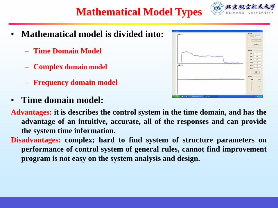
• Mathematical model is divided into:
– Time Domain Model
– Complex domain model
– Frequency domain model
• Time domain model:
Advantages: it is describes the control system in the time domain, and has the
advantage of an intuitive, accurate, all of the responses and can provide
the system time information.
Disadvantages: complex; hard to find system of structure parameters on
performance of control system of general rules, cannot find improvement
program is not easy on the system analysis and design.
Mathematical Model Types

Complex domain models:
It includes the transfer function and structure of the system. It demonstrates
its characteristic of the system and of the input signal;It not only characterize the
dynamic performance of the system, but can also affect the structure or the study of
changes in system parameters on system performance
Frequency domain model:
Describes the frequency characteristics of the system, with a clear
physical meaning, experimental methods are available to determine.
Mathematical Model Types

Relationship between the three commonly used mathematical
models
Linear Systems
Transfer
function
Differential
Equations
Frequency
Characteristics
Rumsfeld
TransformFourier
Transform
Mathematical Model Types

1. A linear system of equations:
① determine the input and output of the system
② The system is divided into several areas, from the input start signal is transmitted in the order, according to the laws of physics followed each variable (Newton's law, Kirchhoff's current and voltage law), etc., lists various aspects of linearization original equation;
2. For the establishment of differential equations, Laplace transform one by one, eliminating the intermediate variables, get the system transfer function model
Modeling steps

Biomimetic robot-DC drive
Mirko Kovac,EPFLSelf-stable system

Biomimetic robot-DC drive
Mirko Kovac,EPFLSelf-stable system
with steering

1Significance of control system simulation
analysis
2
3
4
Modeling methods and procedures
5
DC motor modeling examples
Analysis and correction for linear
motion unit closed-loop
simulation
Introduction to MATLAB /SIMULINK
Contents

19
Solution: armature controlled DC motor is essentially the work of the
input electrical energy into mechanical energy, which is the Input of
the armature voltage Ua (t) generated armature current Ia (t) in the
armature circuit, and then by the current Ia (t) and the excitation flux
generated by the interaction of electromagnetic torque Mm (t), to drag
the load movement. Therefore, the equation of motion of the DC motor
by the following three components.
– Armature circuit voltage balance equation
– Electromagnetic torque equation
– Turn the motor shaft from the balance equation
DC modeling analysis

(1) According to Kirchhoff's voltage law, the armature
winding voltage balance equation
(1)
Where, La and Ra were inductance (Henry) and the resistance of the
armature windings (Ohm)
aa a a a a
diu i R L E
dt
DC modeling analysis

(2) When the rotation of the DC motor armature, the armature
windings produce anti potential, it is generally proportional to
the motor speed, i.e.,
(2)
Where, Ea is the back EMF (V), Ke is a scaling factor (V.rad / s)
ma e
dE K
dt
DC modeling analysis

(3) the interaction between the armature current and the
magnetic field to produce an electromagnetic torque.
General electromagnetic torque is proportional to the armature current,
namely:
Where Mm is the electromagnetic torque (Nm), Ia is the armature current (A),
Km for the moment coefficient (Nm / A)
DC modeling analysis
(3)m m aM K i

(4) for driving the electromagnetic torque to overcome the friction and load
torque, assuming only consider the viscous friction is proportional to the
speed, the DC motor torque balance equation
The formula: J m The total moment of inertia of the motor shaft
(Including the moment of inertia of the rotor and the load)
The angular displacement of the motor shaft (rad);
As a viscous friction coefficient of the motor shaft
The role of the applied load on the motor shaft torque
2
2( )m m
m m m c
d dM J B M t
dt dt
2.. 秒米牛
m
mB
秒/弧度/米.牛
DC modeling analysis
( )cM t

To find the angular velocity and load control model of
the motor armature voltage U, namely the transfer function.
We assume zero initial conditions in these kinds of Laplace
Transform, respectively
m
( )
a a a a a a
a e m
m m a
m m m m c
U s L I s s R I s E s
E s K s
M s K I s
M s J S B s M s
DC modeling analysis

Erasing the armature current ia, and then take the armature
voltage Ua is input, the angular velocity of the motor output shaft,
i.e.,
Whereby the DC motor can be controlled in the model, i.e., the
transfer function is:
2(s)
( )
m m
a a m a m m a a m e m
s K
U s L J s L B J R s R B K K
.m as s U s
m
DC modeling analysis

DC servo motor Structure
DC modeling analysis
Created in MATLAB using the Simulink simulation model

Li Wen et al, Beihang University

DC modeling analysis

Open Simulink
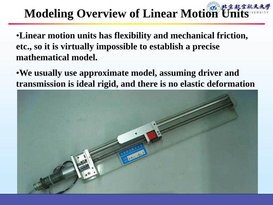
Modeling Overview of Linear Motion Units
•Linear motion units has flexibility and mechanical friction,
etc., so it is virtually impossible to establish a precise
mathematical model.
•We usually use approximate model, assuming driver and
transmission is ideal rigid, and there is no elastic deformation

New Simulink model

The system block diagram of the various
modules and drag it to the model file
Pull in

(2) Linear motion unit components
Ball screw
Coupling
DC motorReducer
Modeling of linear motion unit control system

The system block diagram of the various
modules and drag it to the model file

The system block diagram of all the modules file and drag it to
the model and adjust the layout and orientation

Connection

Variable and label

Substituting parameters La,Ra,Jm,Bm,Km,Ke
• La = 0.001Hery;Ra = 1.2oum;Jm = 1e-5 kg.m2;Bm = 5e-4;Km
= 0.08N.m/A;Ke = 0.08V.S/rad;
Input signal:
• Amplitude of Input voltage Ua is 1V, the frequency of square wave is 1Hz
• Amplitude of the interference torque Mf 0.01Nm, frequency of sinusoidal signal 1Hz
Simulink block diagram to obtain arguments:
DC modeling analysis

matlab m files for variable assignment

Generate input and load (or disturbance torque) signal
generator
Amplitude of Input voltage is Ua 1V, the frequency of square wave is 1Hz
Amplitude of the interference torque Mf 0.01Nm, frequency sinusoidal signal of 1Hz For example: motorSlip ring frictionProduce
Click on Run

Judging from the simulation curve, the response curve is a cycle curve, is in
response to a step input and Input of the linear superposition of the load cycle,
from the curve to see the system is still stable, which can be from the poles
and zeros of the transfer function are located to the left half plane verify get.
DC modeling analysis

Necessary and sufficient conditions for stability of the
system is necessaryAll the roots of the characteristic equation must be negative real part, that is
all the roots in the complex plane of the left half-plane
DC modeling analysis
0.08
G(s) = -------------------------------------------
1e-08 s^2 + 1.25e-05 s + 0.007
Continuous-time transfer function
1
2
625 556i
625 5.56i
Root system characteristics
2 ( )
m m
a a m a m m a a m e m
s C
U s L J s L B J R s R B C C

Jm=10-5
Jm=10-4
DC modeling analysis
Jm=10-3
In three Jm, the system is stable, but smaller overshoot Jm more powerful;
Jm greater the longer the rise time of the system.
Overshoot
Jm Impact on system performance

Bm
=5X10⁻⁴
DC modeling analysis
Bm
=2X10⁻³
Bm
=1X10⁻⁴
Bm impact on performance(Bm bigger (output / input) becomes smaller,
shorter adjustment time)
The greater the damping coefficient, the smaller the value of the unit step response
(speed / voltage value becomes smaller), the rise time becomes longer, but the time
to reach steady state becomes shorter.

DC modeling analysis
Mc = 1Nm
Load impact on performance
Load increase reduce the system response (moving speed), larger changes in the
steady-state error of the system (open-loop steady-state error is large), the
adjustment time becomes longer, the rise time becomes long.
Mc = 2Nm Mc = 3Nm

1Significance of control system simulation
analysis
2
3
4
Modeling methods and procedures
5
DC motor modeling examples
Analysis and correction for linear
motion unit closed-loop
simulation
Introduction to MATLAB /SIMULINK
Contents

Model building
Specify the slider velocity (unit: mm/s) as the input, and the slider
actual speed (mm/s) as the output, establish a mathematic model for
the linear motion unit speed control system.
Modeling Overview of linear motion units

Rated voltage 24VBack-EMF constant
(Ke)0.0307v*s/rad
Reduction ratio (i) 29:1 Amplifier (Ka) 2.4
Motor resistor (Ra) 21.6欧 Torque constant (Km) 0.0307N*m/A
Motor inductance (La) 1.97mHRotor moment of
inertia (Jx)
Screw lead (p) 2mmEquivalent damping
(Bm)0.0005
Screw diameter (d) 11.5mm Speed gain (Ka) 0.0212v*s/rad
Screw Length (L) 540mm
Workbench mass (m) 0.315kg
(1) Linear motion unit system components and parameters
Modeling of linear motion unit control system
7 24.2 10 .kg m
1 1 2 2 2( ) ( )22 4 2 25.362 -7
2e kg m
m xi
d pd l m
J J
Equivalent moment of inertia of the motor shaft

1. The relationship between the motor and the screw speed
The actual relationship between the rotational speed of the motor shaft and the
screw speed: ( i is reduction ratio and the value is 29)
m ot i t
tm
to
Motor shaft speed
Actural speed of screw
Modeling of linear motion unit control system

2. Modeling of DC servo motor
Modeling of linear motion unit control system

2. Modeling of DC servo motor
Potential balance equation of armature windings:
Relations between the counter-electromotive force and speed
The relationship between the armature current and the armature
torque is:
Torque balance equation is:
Modeling of linear motion unit control system

3. Angular velocity feedback
To constitute the load shaft speed control system, there must be speed feedback
of load shaft, the error voltage can be obtained by velocity error:
a a n mu t k t t
n t is the input shaft speed of motor;ak is the speed feedback gain
n t
m t
au tak
Modeling of linear motion unit control system

• Laplace transform of the above formula :
This equation describes the relationship between the input
control voltage U and the rotational angular velocity of the
drive shaft.
m ot i t m os i s
( )m m aM K i N m
( ) aa e m a a a
diu k t L R i
dt
a a n mu t k t t
m m aM s K I s
a a a a a eU s L I s s R I s k s
(s)m m m m m cM s J s s B s M
a a n mu s k s s
(t)(t) J (t) (t)m
m m m m c
dM B M
dt
Modeling of linear motion unit control system

Specify the slider velocity (unit: mm/s) as the input, and the slider
actual speed (mm/s) as the output, establish a mathematic model for
the linear motion unit speed control system. The above notation is
expressed as the angular velocity, as the screw lead P is 2mm, we
can Build relationships between line speed and angular velocity.
P
2
o
o
sV
2
P
oo
Vs
o t is input speed
oV is slider speed
Modeling of linear motion unit control system

Build the system model in Simulink:
Modeling of linear motion unit control system
After determining the mathematical model of the
system, you can use several different methods to
analyze the dynamic performance and steady-state
performance of the control system.
Method:
• Time domain analysis
• Frequency domain analysis.
Simulation analysis of control systems

Dynamic performance and steady-state performance
Simulation analysis of control systems

Input step signal (amplitude is 1) to analyze the time-domain
response
From the results, we can get that rise time, peak time and settling time are
relatively small, although there is a certain system overshoot, but eventually
stabilized, but there is an error between the input and output. Therefore,
system stability and accuracy are not very well.
Simulation analysis of control systems
Simulation analysis of control systems
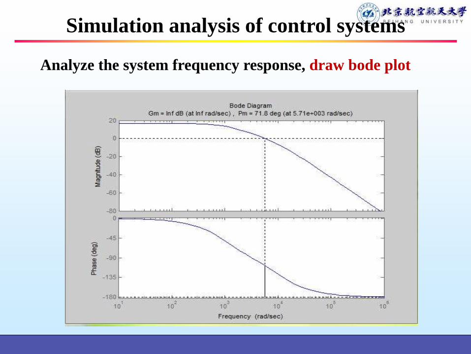
Analyze the system frequency response, draw bode plot
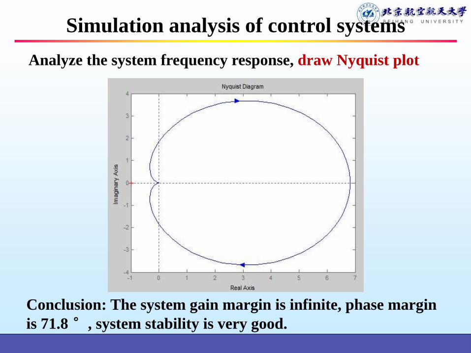
Conclusion: The system gain margin is infinite, phase margin
is 71.8 °, system stability is very good.
Simulation analysis of control systems
Analyze the system frequency response, draw Nyquist plot

6mm
Impacts on system when change parameters
8mm2mm
Impact on the performance of the screw lead
In the open-loop control, when lead increases, changes in steady-state error
is large and the system response increases, rise time get lower.

6mm
8mm
2mm
Impacts on system when change parameters
Impact on the performance of the screw lead
In the open-loop control, changes in lead will not change the dynamic
characteristic.

25 3515
Impact on the performance of the reduction ratio
In the open-loop control, when the reduction ratio increases, system
response time decreases
Impacts on system when change parameters

25
35
15
Impact on the performance of the reduction ratio
Impacts on system when change parameters
In the open-loop control, changes in reduction ratio will not change the
dynamic characteristic.
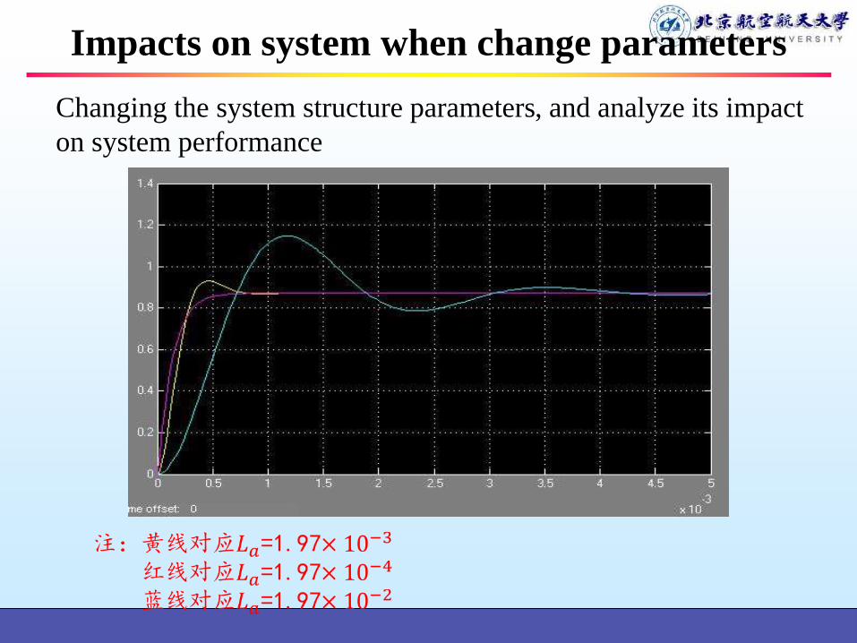
Impacts on system when change parameters
Changing the system structure parameters, and analyze its impact
on system performance
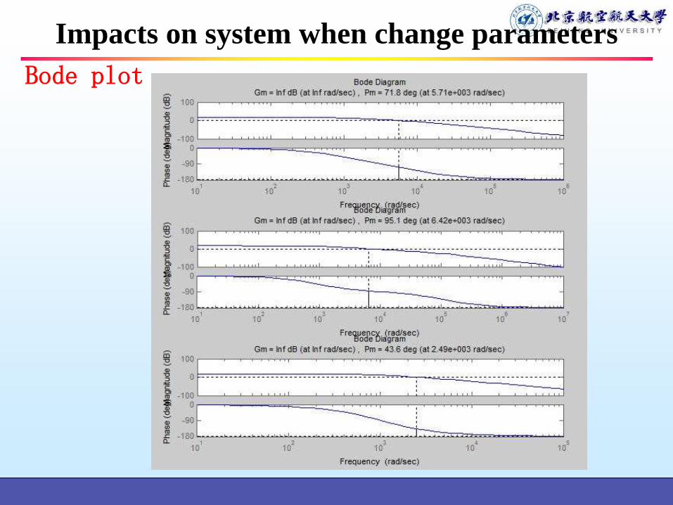
Bode plot
Impacts on system when change parameters

Open Simulink

1Significance of control system simulation
analysis
2
3
4
Modeling methods and procedures
5
DC motor modeling examples
Analysis and correction for linear
motion unit closed-loop
simulation
Introduction to MATLAB /SIMULINK
Contents

biorobotics_fast response
Rob Wood lab, Harvard University
X0.1
Active control

New Simulink model

According to the system block diagram, and drag various modules
to the model file
Drag

According to the system block diagram, and drag various modules
to the model file


Connection

Brought variables and mark

Brought parameters: La,Ra,Jm,Bm,Km,Ke
• La = 0.001H; Ra = 1.2Ω; Jm = 1e-5 kg.m2;Bm = 5e-4;Km = 0.08N.m/A; Ke = 0.08V.S/rad;
Input signal is:
• Square wave: Input voltage Ua is 1V,frequency is 1Hz;
• Sin signal: Disturbance torque Mf is 0.01N.m, frequency is 1Hz;
Simulink block diagram:
DC modeling analysis

Variable assignment in matlab m file
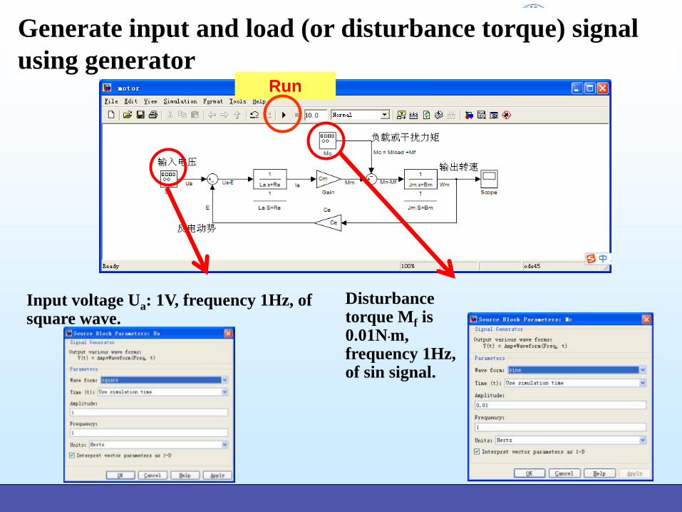
Generate input and load (or disturbance torque) signal
using generator
Input voltage Ua: 1V, frequency 1Hz, of square wave.
Disturbance torque Mf is0.01N.m, frequency 1Hz, of sin signal.
Run

Judging from the simulation curve, the response curve is a cycle curve, which
is a linear superposition response to a step input and periodic load input.
From the curve to see the system is still stable, which can be verified from the
transfer function poles and zeros are in the left half plane.
DC modeling analysis


![[Dag Sorbom] LISREL 8 Structural Equation Modelin(BookFi.org)](https://static.documents.pub/doc/80x56/55cf947f550346f57ba26a7d/dag-sorbom-lisrel-8-structural-equation-modelinbookfiorg.jpg)


