A benchmark for comparison of dental radiography analysis
algorithms
�
Ching-Wei Wang
a , b , ∗, Cheng-Ta Huang
a , b , Jia-Hong Lee
a , b , Chung-Hsing Li c , d , Sheng-Wei Chang
c , Ming-Jhih Siao
c , Tat-Ming Lai e , Bulat Ibragimov
f , Tomaž Vrtovec
f , Olaf Ronneberger g , Philipp Fischer g , Tim F. Cootes h , Claudia Lindner h
a Graduate Institute of Biomedical Engineering, National Taiwan University of Science and Technology, Taiwan b NTUST Center of Computer Vision and Medical Imaging, Taiwan c Orthodontics and Pediatric Dentistry Division, Dental Department, Tri-Service General Hospital, Taiwan d School of Dentistry and Graduate Institute of Dental Science, National Defense Medical Center, Taipei, Taiwan e Department of Dentistry, Cardinal Tien Hospital, Taipei, Taiwan f Faculty of Electrical Engineering, University of Ljubljana, Tržaška 25, SI-10 0 0 Ljubljana, Slovenia g University of Freiburg, Germany h Centre for Imaging Sciences, The University of Manchester, UK
a r t i c l e i n f o
Article history:
Received 8 September 2015
Revised 2 February 2016
Accepted 19 February 2016
Available online 28 February 2016
Keywords:
Cephalometric tracing
Anatomical segmentation and classification
Bitewing radiography analysis
Challenge and benchmark
a b s t r a c t
Dental radiography plays an important role in clinical diagnosis, treatment and surgery. In recent years,
efforts have been made on developing computerized dental X-ray image analysis systems for clinical us-
ages. A novel framework for objective evaluation of automatic dental radiography analysis algorithms
has been established under the auspices of the IEEE International Symposium on Biomedical Imaging
Eight standard clinical measurement methods for classification of anatomical types.
Method (1) ANB (2) SNB (3) SNA (4) ODI (5) APDI (6) FHI (7) FHA (8) MW
Type 1 3.2 ° ∼ 5.7 °Class I (normal)
74.6 ° ∼ 78.7 °Normal
mandible
79.4 ° ∼ 83.2 °Normal maxilla
Normal: 74.5 °± 6.07 °
Normal: 81.4 °± 3.8 °
Normal: 0.65
∼ 0.75
Normal: 26.8 °∼ 31.4 °
Type 1: Normal:
2 mm ∼ 4.5 mm
Type 2 > 5.7 ° Class II < 74.6 °Retrognathic
mandible
> 83.2 °Prognathic
maxilla
> 80.5 ° Deep
bite tendency
< 77.6 ° Class II
tendency
> 0.75 Short
face tendency
> 31.4 °Mandible high
angle tendency
Type 2: MW = 0
mm Edge to edge
Type 3: MW < 0
mm Anterior
cross bite
Type 3 < 3.2 ° Class III > 78.7 °Prognathic
mandible
< 79.4 °Retrognathic
maxilla
< 68.4 ° Open
bite tendency
> 85.2 ° Class III
tendency
< 0.65 Long
face tendency
< 26.8 °Mandible lower
angle tendency
Type 4: MW > 4.5
mm Large over
jet
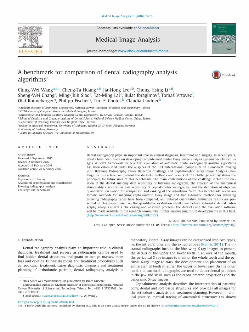
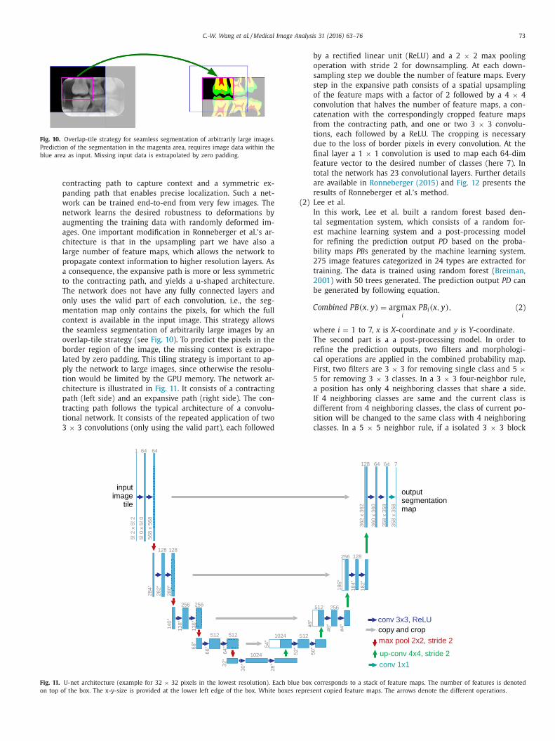
Fig. 2. Bitewing radiographs: (a) a raw image with (b) seven dental structures highlighted, including (1) caries with blue color, (2) enamel with green color, (3) dentin with
yellow color, (4) pulp with red color, (5) crown with skin color, (6) restoration with orange color and (7) root canal treatment with cyan color. The images are captured
using the SOREDEX system (SOREDEX, Finland), that is devised with an optional image plate identification system (IDOT) for quality control, and ’C3’ on the image indicates
the active/frontal side in the IDOT system.
l
t
s
t
t
n
t
c
l
1
a
s
t
w
r
d
m
a
o
t
m
2
I
a
2
s
a
a
andmarks to be detected on lateral cephalograms are the sella,
he nasion, the orbitale, the porion, the subspinale (A point), the
upramentale (B point), the pogonion, the menton, the gnathion,
he gonion, the lower incisal incision, the upper incisal incision,
he upper lip, the lower lip, the subnasal, the soft tissue pogo-
ion, the posterior nasal spine, the anterior nasal spine, the an-
erior nasal spine and the articulare as shown in Fig. 1 (a). For the
lassification of anatomical types based on the obtained anatomical
andmarks, eight standard clinical measurement methods ( Downs,
948; Kim, 1974; Kim and Vietas, 1978; McNamara, 1984; Nanda
nd Nanda, 1969; Steiner, 1953; Tweed, 1946 ) were included as
hown in Table 2 and illustrated in Fig. 1 (b)–(d). For the analysis of
he dental anatomy of bitewing radiographs, seven tooth structures
ere included: caries, enamel, dentin, pulp, crown, restoration, and
oot canal treatment (see Fig. 2 ).
There were two stages in both challenges. In stage 1, a training
ataset and a first test dataset were released for method develop-
ent. In stage 2, an on-site competition was organized for which
second test dataset was used. The results of all individual meth-
ds were compared to the ground truth data, and extensive quan-
itative evaluation was performed to assess the performance of all
ethods.
.2. Participants
A total of 18 teams (from 12 countries) registered for the 2015
EEE ISBI grand challenge, and the four teams listed below were
ccepted in stage 1 and invited to the on-site competition in stage
. The four approaches are described in Sections 3.1 and 4.1 , re-
pectively. In landmark detection of cephalometric radiographs, we
lso compare five methods submitted to the 2014 ISBI challenge,
nd details of the five methods can be referred to ( Wang, 2015 ).
(1) Ibragimov et al., computerized cephalometry by game the-
ory with shape- and appearance-based landmark refinement
(Slovenia).
66 C.-W. Wang et al. / Medical Image Analysis 31 (2016) 63–76
Table 3
Image distribution in the training, Test1 and Test2 data.
(2) Lindner and Cootes, fully automatic cephalometric evalua-
tion using random forest regression-voting (UK).
(3) Lee et al., dental X-ray image segmentation using random
forest (Taiwan).
(4) Ronneberger et al., dental X-ray image segmentation using a
U-shaped deep convolutional network (Germany).
2.3. Datasets
400 cephalometric radiographs were collected from 400 pa-
tients aged six to 60 years. The cephalograms were acquired in
TIFF format with Soredex CRANEXr Excel Ceph machine (Tuusula,
Finland) and Soredex SorCom software (3.1.5, version 2.0), and the
image resolution was 1935 × 2400 pixels. For evaluation, 19 land-
marks were manually marked in each image and reviewed by two
experienced medical doctors; the ground truth is the average of
the markups by both doctors. For the classifications of anatomical
types, eight clinical measurement methods were used (see illustra-
tions in Fig. 1 and classifications in Table 2 ) :
1. ANB = � L 5 L 2 L 6 , the angle between the landmark 5, 2 and 6
2. SNB = � L 1 L 2 L 6 ;
3. SNA = � L 1 L 2 L 5 4. ODI = ∠ L 5 L 6 L 8 L 10 + L 17 L 18 L 4 L 3 , the arithmetic sum of the angle
between the AB plane ( L 5 L 6 ) to the Mandibular Plane (MP,
L 8 L 10 )and the angle of the Palatal Plane (PP, L 17 L 18 ) to Frankfort
Horizontal plane (FH, L 4 L 3 )
5. APDI = L 3 L 4 L 2 L 7 + L 2 L 7 L 5 L 6 + L 3 L 4 L 17 L 18
6. FHI = L 1 L 10 / L 2 L 8 , the ratio of the Posterior Face Height (PFH =the distance from L 1 to L 10 ) to the Anterior Face Height (AFH =the distance from L 2 to L 8 )
7. FHA = ∠ L 1 L 2 L 10 L 9 8. MW = | L 12 L 11 | where x ( L 12 ) > x ( L 11 ), otherwise, MW = −| L 12 L 11 |
For the bitewing radiography analysis, 120 images were col-
lected from 120 patients, acquired in TIFF format with Sirona HE-
LIODENT DS SIDEXIS machine (Salzburg, Austria) and EBM Viewer
software (version 4.2c). For evaluation, seven types were manually
marked in each image and reviewed by two experienced medical
doctors.
Both datasets were randomly divided into three subsets as
Training data, Test1 data and Test2 data for two stage testing (see
Table 3 ). Ethical approval (IRB Number 1-102-05-017) was obtained
to conduct the study by the research ethics committee of the Tri-
Service General Hospital in Taipei, Taiwan. The datasets and the
evaluation software will be made available to the research commu-
nity, further encouraging future developments in this field. ( http:
//www-o.ntust.edu.tw/ ∼cweiwang/ISBI2015/ ).
2.4. Evaluation approaches
In cephalometric radiography analysis, three main criteria are
used to evaluate the performance of the submitted methods.
• Mean radial error
The radial error R is formulated as R =
√
� x 2 + � y 2 , where � x
is the absolute distance in the x-direction between the obtained
landmark and the referenced landmark, and � y is the absolute
distance in the y-direction between the obtained landmark and
the referenced landmark. The mean radial error (MRE) and the
associated standard deviation (SD) are defined as MRE =
∑ N i =1 R i N
and SD =
√ ∑ N i =1 (R i −MRE) 2
N−1 .
• Success detection rate
For each landmark, medical doctors mark the location of a sin-
gle pixel instead of an area as a referenced landmark location.
If the absolute difference between the detected landmark and
the referenced landmark is no greater than z mm, the detec-
tion of this landmark is considered as a successful detection;
otherwise, it is considered as a misdetection. The success de-
tection rate p z with precision less than z mm is formulated as
p z =
# { j : ‖ L d ( j ) −L r ( j ) ‖ <z} #� × 100% , where L d , L r represent the loca-
tion of the detected landmark and the referenced landmark, re-
spectively; z denotes four precision measurements used in the
evaluation, including 2 mm, 2.5 mm, 3 mm and 4 mm; j ∈ �,
and #� represents the number of detections made. • Confusion matrix and success classification rate
In the confusion matrix, each column of the matrix represents
the instances of a predicted class, while each row represents
the instances of the ground truth class. The averaged diagonal
of a confusion matrix represents the success classification rate.
Confusion matrices also provide valuable information on where
misclassifications occur.
In bitewing radiography analysis, three main criteria are used
o evaluate the performance of submitted methods, including Sen-
C.-W. Wang et al. / Medical Image Analysis 31 (2016) 63–76 67
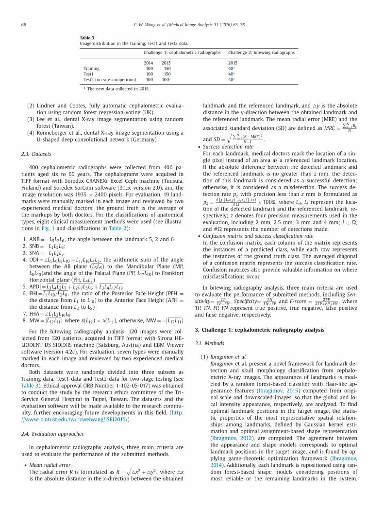
Fig. 3. (a) An illustration of the multi-scale appearance model that captures global
appearance (top) and local appearance (bottom) of the target landmark (green cir-
cle). (b) An illustration of the shape model, where the position of the target land-
mark (green circle) is defined using the position of the remaining landmarks (yel-
low circles). (For interpretation of the references to color in this figure legend, the
reader is referred to the web version of this article.)
3
g
T
Fig. 3 shows the illustrations of the multi-scale appearance
model and the shape model.
(2) Lindner and Cootes
Recent work has shown that one of the most effective ap-
proaches to detect a set of landmark positions on an ob-
ject of interest is to train Random Forests (RFs) to vote for
the likely position of each landmark, then to find the shape
model parameters which optimize the total votes over all
landmark positions. Lindner and Cootes apply Random For-
est regression-voting in the Constrained Local Model frame-
work (RFRV-CLM) ( Lindner, 2015 ) as part of a fully auto-
matic landmark detection system ( Lindner, 2013 ) to detect
the 19 landmarks on new unseen images. In the RFRV-CLM
approach, a RF is trained for each landmark to learn to pre-
dict the likely position of that landmark. During detection,
a statistical shape model (( Cootes, 1995 ) is matched to the
predictions over all landmark positions to ensure consis-
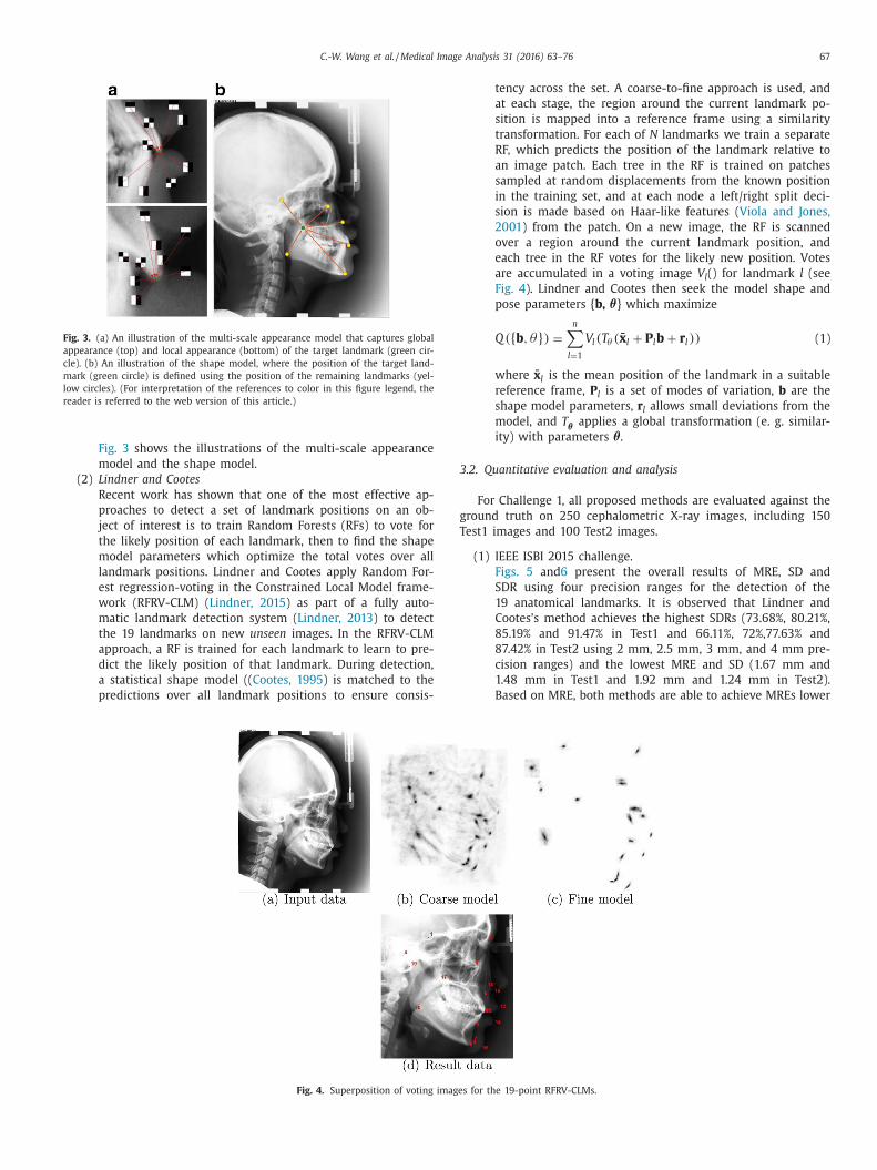
Fig. 4. Superposition of voting image
tency across the set. A coarse-to-fine approach is used, and
at each stage, the region around the current landmark po-
sition is mapped into a reference frame using a similarity
transformation. For each of N landmarks we train a separate
RF, which predicts the position of the landmark relative to
an image patch. Each tree in the RF is trained on patches
sampled at random displacements from the known position
in the training set, and at each node a left/right split deci-
sion is made based on Haar-like features ( Viola and Jones,
2001 ) from the patch. On a new image, the RF is scanned
over a region around the current landmark position, and
each tree in the RF votes for the likely new position. Votes
are accumulated in a voting image V l () for landmark l (see
Fig. 4 ). Lindner and Cootes then seek the model shape and
pose parameters { b, θ} which maximize
Q({ b , θ} ) =
n ∑
l=1
V l (T θ ( ̄x l + P l b + r l )) (1)
where x̄ l is the mean position of the landmark in a suitable
reference frame, P l is a set of modes of variation, b are the
shape model parameters, r l allows small deviations from the
model, and T θ applies a global transformation (e. g. similar-
ity) with parameters θ.
.2. Quantitative evaluation and analysis
For Challenge 1, all proposed methods are evaluated against the
round truth on 250 cephalometric X-ray images, including 150
est1 images and 100 Test2 images.
(1) IEEE ISBI 2015 challenge.
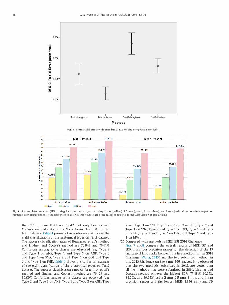
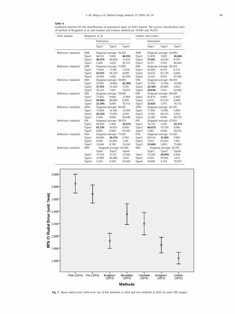
Figs. 5 and 6 present the overall results of MRE, SD and
SDR using four precision ranges for the detection of the
19 anatomical landmarks. It is observed that Lindner and
Cootes’s method achieves the highest SDRs (73.68%, 80.21%,
85.19% and 91.47% in Test1 and 66.11%, 72%,77.63% and
87.42% in Test2 using 2 mm, 2.5 mm, 3 mm, and 4 mm pre-
cision ranges) and the lowest MRE and SD (1.67 mm and
1.48 mm in Test1 and 1.92 mm and 1.24 mm in Test2).
Based on MRE, both methods are able to achieve MREs lower
s for the 19-point RFRV-CLMs.
68 C.-W. Wang et al. / Medical Image Analysis 31 (2016) 63–76
Fig. 5. Mean radial errors with error bar of two on-site competition methods.
Fig. 6. Success detection rates (SDRs) using four precision ranges, including 2 mm (yellow), 2.5 mm (green), 3 mm (blue) and 4 mm (red), of two on-site competition
methods. (For interpretation of the references to color in this figure legend, the reader is referred to the web version of this article.)
than 2.5 mm on Test1 and Test2, but only Lindner and
Cootes’s method obtains the MREs lower than 2.0 mm on
both datasets. Table 4 presents the confusion matrices of the
eight classifications of the anatomical types on Test1 dataset.
The success classification rates of Ibragimov et al.’s method
and Lindner and Cootes’s method are 70.84% and 76.41%.
Confusions among some classes are observed (e.g. Type 2
and Type 1 on ANB, Type 1 and Type 3 on ANB, Type 2
and Type 1 on SNA, Type 3 and Type 1 on ODI, and Type
2 and Type 1 on FHI). Table 5 shows the confusion matrices
of the eight classification of the anatomical types on Test2
dataset. The success classification rates of Ibragimov et al.’s
method and Lindner and Cootes’s method are 76.12% and
80.99%. Confusions among some classes are observed (e.g.
Type 2 and Type 1 on ANB, Type 1 and Type 3 on ANB, Type
2 and Type 1 on SNB, Type 1 and Type 3 on SNB, Type 2 and
Type 1 on SNA, Type 2 and Type 1 on ODI, Type 1 and Type
3 on FHI, Type 1 and Type 2 on FHA, and Type 4 and Type
1 on MW).
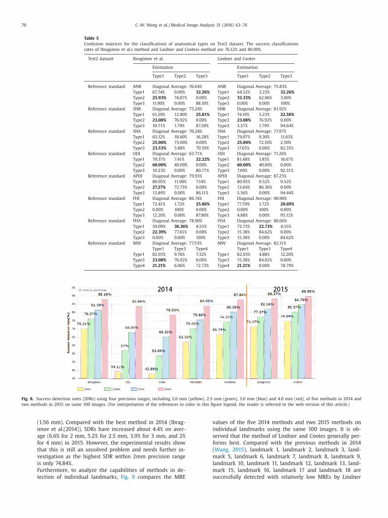
(2) Compared with methods in IEEE ISBI 2014 Challenge
Figs. 7 and 8 compare the overall results of MRE, SD and
SDR using four precision ranges for the detection of the 19
anatomical landmarks between the five methods in the 2014
Challenge ( Wang, 2015 ) and the two submitted methods in
this 2015 Challenge on the same 100 images. It is observed
that the two methods, submitted in 2015, are better than
all the methods that were submitted in 2014. Lindner and
Cootes’s method achieves the highest SDRs (74.84%, 80.37%,
84.79%, and 89.95%) using 2 mm, 2.5 mm, 3 mm, and 4 mm
precision ranges and the lowest MRE (1.656 mm) and SD
C.-W. Wang et al. / Medical Image Analysis 31 (2016) 63–76 69
Table 4
Confusion matrices for the classifications of anatomical types on Test1 dataset. The success classification rates
of method of Ibragimov et al. and Lindner and Cootess method are 70.84% and 76.41%.
Test1 dataset Ibragimov et al. Lindner and Cootes
Estimation Estimation
Type1 Type2 Type3 Type1 Type2 Type3
Reference standard ANB Diagonal average: 59.42% ANB Diagonal average: 64.99%
Fig. 8. Success detection rates (SDRs) using four precision ranges, including 2.0 mm (yellow), 2.5 mm (green), 3.0 mm (blue) and 4.0 mm (red), of five methods in 2014 and
two methods in 2015 on same 100 images. (For interpretation of the references to color in this figure legend, the reader is referred to the web version of this article.)
(1.56 mm). Compared with the best method in 2014 (Ibrag-
imov et al.(2014)), SDRs have increased about 4.4% on aver-
age (6.6% for 2 mm, 5.2% for 2.5 mm, 3.9% for 3 mm, and 2%
for 4 mm) in 2015. However, the experimental results show
that this is still an unsolved problem and needs further in-
vestigation as the highest SDR within 2mm precision range
is only 74.84%.
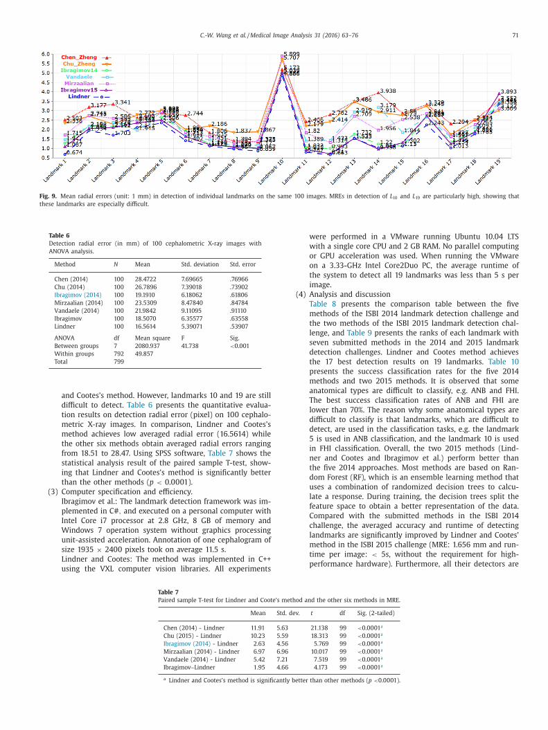
Furthermore, to analyze the capabilities of methods in de-
tection of individual landmarks, Fig. 9 compares the MRE
values of the five 2014 methods and two 2015 methods on
individual landmarks using the same 100 images. It is ob-
served that the method of Lindner and Cootes generally per-
forms best. Compared with the previous methods in 2014
mark 15, landmark 16, landmark 17 and landmark 18 are
successfully detected with relatively low MREs by Lindner
C.-W. Wang et al. / Medical Image Analysis 31 (2016) 63–76 71
Fig. 9. Mean radial errors (unit: 1 mm) in detection of individual landmarks on the same 100 images. MREs in detection of L 10 and L 19 are particularly high, showing that
these landmarks are especially difficult.
Table 6
Detection radial error (in mm) of 100 cephalometric X-ray images with
ANOVA analysis.
Method N Mean Std. deviation Std. error
Chen (2014) 100 28.4722 7.69665 .76966
Chu (2014) 100 26.7896 7.39018 .73902
Ibragimov (2014) 100 19.1910 6.18062 .61806
Mirzaalian (2014) 100 23.5309 8.47840 .84784
Vandaele (2014) 100 21.9842 9.11095 .91110
Ibragimov 100 18.5070 6.35577 .63558
Lindner 100 16.5614 5.39071 .53907
ANOVA df Mean square F Sig.
Between groups 7 2080.937 41.738 < 0.001
Within groups 792 49.857
Total 799
and Cootes’s method. However, landmarks 10 and 19 are still
difficult to detect. Table 6 presents the quantitative evalua-
tion results on detection radial error (pixel) on 100 cephalo-
metric X-ray images. In comparison, Lindner and Cootes’s
method achieves low averaged radial error (16.5614) while
the other six methods obtain averaged radial errors ranging
from 18.51 to 28.47. Using SPSS software, Table 7 shows the
statistical analysis result of the paired sample T-test, show-
ing that Lindner and Cootes’s method is significantly better
than the other methods ( p < 0.0 0 01).
(3) Computer specification and efficiency.
Ibragimov et al.: The landmark detection framework was im-
plemented in C # , and executed on a personal computer with
Intel Core i7 processor at 2.8 GHz, 8 GB of memory and
Windows 7 operation system without graphics processing
unit-assisted acceleration. Annotation of one cephalogram of
size 1935 × 2400 pixels took on average 11.5 s.
Lindner and Cootes: The method was implemented in C++
using the VXL computer vision libraries. All experiments
Table 7
Paired sample T-test for Lindner and Coote’s me
Mean Std.
Chen (2014) - Lindner 11 .91 5 .63
Chu (2015) - Lindner 10 .23 5 .59
Ibragimov (2014) - Lindner 2 .63 4 .56
Mirzaalian (2014) - Lindner 6 .97 6 .96
Vandaele (2014) - Lindner 5 .42 7 .21
Ibragimov–Lindner 1 .95 4 .66
a Lindner and Cootes’s method is significantly
were performed in a VMware running Ubuntu 10.04 LTS
with a single core CPU and 2 GB RAM. No parallel computing
or GPU acceleration was used. When running the VMware
on a 3.33-GHz Intel Core2Duo PC, the average runtime of
the system to detect all 19 landmarks was less than 5 s per
image.
(4) Analysis and discussion
Table 8 presents the comparison table between the five
methods of the ISBI 2014 landmark detection challenge and
the two methods of the ISBI 2015 landmark detection chal-
lenge, and Table 9 presents the ranks of each landmark with
seven submitted methods in the 2014 and 2015 landmark
detection challenges. Lindner and Cootes method achieves
the 17 best detection results on 19 landmarks. Table 10
presents the success classification rates for the five 2014
methods and two 2015 methods. It is observed that some
anatomical types are difficult to classify, e.g. ANB and FHI.
The best success classification rates of ANB and FHI are
lower than 70%. The reason why some anatomical types are
difficult to classify is that landmarks, which are difficult to
detect, are used in the classification tasks, e.g. the landmark
5 is used in ANB classification, and the landmark 10 is used
in FHI classification. Overall, the two 2015 methods (Lind-
ner and Cootes and Ibragimov et al.) perform better than
the five 2014 approaches. Most methods are based on Ran-
dom Forest (RF), which is an ensemble learning method that
uses a combination of randomized decision trees to calcu-
late a response. During training, the decision trees split the
feature space to obtain a better representation of the data.
Compared with the submitted methods in the ISBI 2014
challenge, the averaged accuracy and runtime of detecting
landmarks are significantly improved by Lindner and Cootes’
method in the ISBI 2015 challenge (MRE: 1.656 mm and run-
time per image: < 5s, without the requirement for high-
performance hardware). Furthermore, all their detectors are
thod and the other six methods in MRE.
dev. t df Sig. (2-tailed)
21 .138 99 < 0.0 0 01 a
18 .313 99 < 0.0 0 01 a
5 .769 99 < 0.0 0 01 a
10 .017 99 < 0.0 0 01 a
7 .519 99 < 0.0 0 01 a
4 .173 99 < 0.0 0 01 a
better than other methods ( p < 0.0 0 01).
72 C.-W. Wang et al. / Medical Image Analysis 31 (2016) 63–76
Table 8
Comparison table for the seven accepted methods of the 2014 and 2015 automated landmark detection challenges.
Method (year) Base method Features Average ranking
(MRE value)
Chen and Zheng (2014) Voting •Sparse shape composition model 7 (2.847) •Voting strategy
Chu et al. (2014) Random forest •Landmark correction: sparse shape composition model 6 (2.679)
Ibragimov et al. (2014) (best
method in 2014)
Random forest •Haar-like features 3 (1.919)
•Game theory •Spatial relationships among pairs of landmarks, modeled by Gaussian kernel density
estimation.
Mirzaalian and Hamarneh
(2014)
Random forest •A pictorial structure algorithm with data likelihood and regularization energy terms. 5 (2.353)
Vandaele et al. (2014) Extremely randomized
trees
•Training pixels are randomly extracted in a radius of at most 4 cm to the landmark. 4 (2.198)
•All method parameters are tuned via 10-fold cross-validation.
Ibragimov et al. (2015) Random forest •Pairwise spatial relationships among landmarks through the optimal
assignment-based shape representation
2 (1.851)
•Multi-landmark spatial relationships through the random forest-based representation •Haar-like appearance features •Game theory
Lindner and Cootes (2015)
(best method in 2015)
Random forest •Regression-voting 1 (1.656)
•Constrained local model framework •Houghforests.
Table 9
The ranking of each landmark for the seven accepted methods in the 2014 and 2015 automated landmark detection challenges.
Method L 1 L 2 L 3 L 4 L 5 L 6 L 7 L 8 L 9 L 10 L 11 L 12 L 13 L 14 L 15 L 16 L 17 L 18 L 19 #Rank1
Average 0.419 0.195 0.531 0.497 0.982 0.913 0.525 0.287
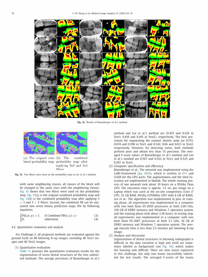
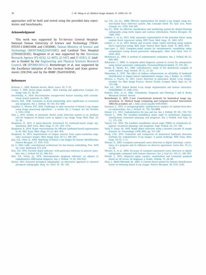
Fig. 14. Six samples of seven dental structures in bitewing radiography with raw image (left side) and manual segmentation result (right side).
5
f
c
s
p
t
c
a
d
d
i
w
d
i
o
o
a
t
r
w
m
(Ronneberger et al. and Lee et al.) are 0.560 and 0.268, re-
spectively, and the u-shaped deep convolutional network by
Ronneberger et al. performs significantly better and achieves
F-scores greater than 0.7 for the three fundamental den-
tal structures ( enamel, dentin and pulp ). The main advantage
of the u-net architecture for this task is its ability to au-
tomatically learn the hierarchical structure within the im-
ages. During segmentation it uses the extracted context at
all detail levels for the decision at each pixel. A critical part
of Ronneberger et al.’s approach is data augmentation. As
there is limited data available, Ronneberger et al. use data
augmentation by applying elastic deformations to produce
a large database with 20 0 0 0 training image tiles, which is
essential for machine learning methods to learn invariance
and produce robust models. The value of data augmenta-
tion for learning invariance has also been shown in Dosovit-
skiy et al. ( Dosovitskiy, 2014 ) in the scope of unsupervised
feature learning. In the experiments, it is observed that the
data augmentation technique helps to create reasonable ad-
ditional training instances for enamel, dentin and pulp, but
the other classes caries, crown, restoration and root canal
treatment, appear quite different according to their relative
location, so the augmentation is less successful here.
. Conclusion
Computerized automatic dental radiography analysis systems
or clinical use save time and manual costs and avoid problems
aused by intra- and inter-observer variations e.g. due to fatigue,
tress or different levels of experience. In this article, we have
resented benchmarks for a number of challenging tasks in den-
al X-ray image analysis, including algorithms for (i) anatomi-
al landmark detection on lateral cephalometric radiographs, (ii)
natomical abnormality classification on lateral cephalometric ra-
iographs, and (iii) dental structure segmentation on bitewing ra-
iographs. The presented results will allow the objective compar-
son of existing and new developments in the field. All methods
ere evaluated using a common lateral cephalometric radiography
ataset repository, a common bitewing radiography dataset repos-
tory, ground truth data, and unified measurements for assessment
f the detection, classification and segmentation accuracy. Based
n the presented results, we can conclude that recent methods
chieved significantly improved performance on these challenging
asks. However, the presented results also demonstrate that accu-
ately analyzing dental radiographs remains a challenging problem
hich is still far from being solved. It is expected that this bench-
ark will help algorithmic developments, and that more advanced
76 C.-W. Wang et al. / Medical Image Analysis 31 (2016) 63–76
L
L
L
L
L
M
N
N
N
O
R
R
R
S
S
T
T
V
W
W
Z
approaches will be built and tested using the provided data repos-
itories and benchmarks.
Acknowledgment
This work was supported by Tri-Service General Hospital-
National Taiwan University of Science and Technology (TSGH-
NTUST-C104011008 and C103008), Taiwan Ministry of Science and
Technology ( MOST1042221E011085 ) and Cardinal Tien Hospital
(CTH10212C02). Ibragimov et al. was supported by the Slovenian
Research Agency ( P2-0232, L2-4072, J2-5473 and J7-6781 ). C. Lind-
ner is funded by the Engineering and Physical Sciences Research
Council , UK ( EP/M012611/1 ). Ronneberger et al. was supported by
the Excellence Initiative of the German Federal and State govern-
ments (EXC294) and by the BMBF (Fkz0316185B).
References
Breiman, L. , 2001. Random forests. Mach. Learn. 45, 5–32 .
Cootes, T. , 1995. Active shape models - their training and application. Comput. Vis.Image Und. 61, 38–59 .
Dosovitskiy, A. , 2014. Discriminative unsupervised feature learning with convolu-tional neural networks. In: NIPS .
Downs, W.B. , 1948. Variations in facial relationship, their significance in treatment
and prognosis. Am. J. Orthod. 34 (10), 812–840 . Gayathri, V. , Menon, H.P. , 2014. Challenges in edge extraction of dental x-ray images
using image processing algorithms - a review. Int. J. Comput. Sci. Inf. Technol.5, 5355–5358 .
Huh, J. , 2015. Studies of automatic dental cavity detection system as an auxiliarytool for diagnosis of dental caries in digital x-ray image. Progr. Med. Phys. 25,
52–58 .
Ibragimov, B. , 2012. A game-theoretic framework for landmark-based image seg-mentation. IEEE Trans. Med. Imag. 31 (9), 1761–1776 .
Ibragimov, B. , 2014. Shape representation for efficient landmark-based segmentationin 3d. IEEE Trans. Med. Imag. 33 (4), 861–874 .
Ibragimov, B. , 2015. Segmentation of tongue muscles from super-resolution mag-netic resonance images. Med. Image Anal. 20 (1), 198–207 .
Jain, A.K. , Chen, H. , 2004. Matching of dental x-ray images for human identification.
Pattern Recognit. 37, 1519–1532 . Jia, Y. , 2014. Caffe: convolutional architecture for fast feature embedding. Proc. ACM
Int. Conf. Multimed. 675–678 . Kim, Y.H. , 1974. Overbite depth indicator: with particular reference to anterior open-
bite. Am. J. Orthod. 65 (6), 586–611 . Kim, Y.H. , Vietas, J.J. , 1978. Anteroposterior dysplasia indicator: an adjunct to
cephalometric differential diagnosis. Am. J. Orthod. 73 (6), 619–633 . Kumar , 2011. Extraoral periapical radiography: an alternative approach to intraoral
cNamara, J.J. , 1984. A method of cephalometric evaluation. Am. J. Orthod. 86 (6),449–469 .
akamoto, T. , 2008. A computer-aided diagnosis system to screen for osteoporosis
using dental panoramic radiographs. Dentomaxillofacial Radiol. 37, 274–281 . anda, R. , Nanda, R.S. , 1969. Cephalometric study of the dentofacial complex of
north indians. Angl. Orthod. 39 (1), 22–28 . ikneshan, S. , 2015. The effect of emboss enhancement on reliability of landmark
identification in digital lateral cephalometric images. Iran. J. Radiol. 12, e19302 . liveira, J. , Proenc, H. , 2011. Caries detection in panoramic dental x-ray images.
mentation. In: Medical Image Computing and Computer-Assisted Intervention
(MICCAI) . accepted, url = http://arxiv.org/abs/1505.04597. assouni, V. , 1955. A roentgenographic cephalometric analysis of cephalo-facio-den-
tal relationships. Am. J. Orthod. 41, 735–764 . 1955 teiner, C.C. , 1953. Cephalometrics for you and me. Am. J. Orthod. 39 (10), 729–755 .
weed, C. , 1946. The frankfort-mandibular plane angle in orthodontic diagnosis,classification, treatment planning, and prognosis. Am. J. Orthod. Oral Surg. 32
(1), 175–230 .
weed, C.H. , 1954. The frankfort mandibular incisal angle (FMIA) in orthodontic di-agnosis, treatment planning, and prognosis. Angl. Orthod. 24, 121–169 .
iola, P. , Jones, M. , 2001. Rapid object detection using a boosted cascade of simplefeatures. In: Proceedings CVPR 2001, pp. 511–518 .
ang, C.W. , 2015. Evaluation and comparison of anatomical landmark detectionmethods for cephalometric X-ray images: A grand challenge. IEEE Trans. Med.
Imag. 34 (9), 1–11 .
Wenzel, A. , 2001. Computer-automated caries detection in digital bitewings: consis-tency of a program and its influence on observer agreement. Caries Res. 35 (1),
12–20 . enzel, A. , et al. , 2002. Accuracy of computer-automated caries detection in digital
radiographs compared with human observers. Eur. J. Oral Sci. 110 (3), 199–203 . Wriedt, S. , 2012. Impacted upper canines: examination and treatment proposal
based on 3d versus 2d diagnosis. J. Orofac. Orthop. 73, 28–40 . hou, J. , Abdel-Mottaleb, M. , 2005. A content-based system for human identification
based on bitewing dental X-ray images. Pattern Recognit. 38, 2132–2142 .


![Journal of Chemournal of Chemical Sciences Volume 104 ical Sciences Volume 104 Issue 2 1992 [Doi 10.1007%2Fbf02863363] M S a Abdel-Mottaleb; M S Antonious; M M Abo Ali; L F M Ismail;](https://static.documents.pub/doc/80x56/577cc3d01a28aba711974656/journal-of-chemournal-of-chemical-sciences-volume-104-ical-sciences-volume.jpg)


