Princeton Companion to Applied Mathematics Proof 1

Medical ImagingCharles L. Epstein

1 Introduction

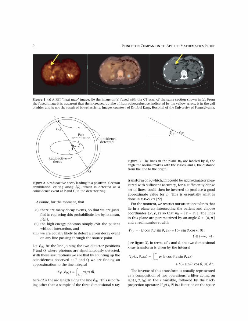
Over the past fifty years the processes and techniquesof medical imaging have undergone a veritable explo-sion, calling into service increasingly sophisticatedmathematical tools. Mathematics provides a languageto describe the measurement processes that lead, even-tually, to algorithms for turning the raw data intohigh-quality images. There are four principal modali-ties in wide application today: x-ray computed tomog-raphy (x-ray CT), ultrasound, magnetic resonance imag-ing (MRI), and emission tomography (positron emissiontomography (PET) and single-photon emission com-puted tomography (SPECT)). Each modality uses a dif-ferent physical process to produce image contrast: x-ray CT produces a map of the x-ray attenuation coeffi-cient, which is strongly correlated with density; ultra-sound images are produced by mapping absorptionand reflection of acoustic waves; in their simplest form,magnetic resonance images show the density of waterprotons, but the subtlety of the underlying physics pro-vides many avenues for producing clinically meaning-ful contrasts in this modality; PET and SPECT give spa-tial maps of the chemical activity of metabolites, whichare bound to radioactive elements. It has recently beenfound useful to merge different modalities. For exam-ple, a fused MRI/PET image shows metabolic activityproduced by PET, at a fairly low spatial resolution,against the background of a detailed anatomic imageproduced by MRI. Figure 1 shows a PET image, a PETimage fused with a CT image, and the CT image as well.

In this article we consider mathematical aspectsof PET, whose underlying physics we briefly explain.Positron emission is a mode of radioactive decay stem-ming from the reaction

proton → neutron+ positron+ neutrino+ energy. (1)

Two isotopes, of clinical importance, that undergo thistype of decay are F18 and C11. The positron, whichis the positively charged antiparticle of the electron,is typically very short-lived as it is annihilated, alongwith the first electron it encounters, producing a pairof 0.511 MeV photons. This usually happens within amillimeter or two of the site of the radioactive decay.Due to conservation of momentum, these two photonstravel in nearly opposite directions along a straight line

(see figure 2). The phenomenon of pair annihilationunderlies the operation of a PET scanner.

A short-lived isotope that undergoes the reactionin (1) is incorporated into a metabolite, e.g., fluo-rodeoxyglucose, which is then injected into the patient.This metabolite is taken up differentially by vari-ous structures in the body. For example, many typesof cancerous tumors have a very rapid metabolismand quickly take up available fluorodeoxyglucose. Thedetector in a PET scanner is a ring of scintillation crys-tals that surrounds some portion of the patient. Thehigh-energy photon interacts with the crystal to pro-duce a flash of light. These flashes are fed into photo-multiplier tubes with electronics that localize, to someextent, where the flash of light occurred and measurethe energy of the photon that produced it. Finally, dif-ferent arrival times are compared to determine whichevents are likely to be “coincidences,” caused by a sin-gle pair annihilation. Two photons detected within atime window of about 10 nanoseconds are assumedto be the result of a single annihilation event. Themeasured locations of a pair of coincident photonsthen determines a line. If the photons simply exitedthe patient’s body without further interactions, thenthe annihilation event must have occurred somewherealong this line (see figure 2). It is not difficult to imag-ine that sufficiently many such measurements could beused to reconstruct an approximation for the distribu-tion of sources, a goal which is facilitated by a morequantitative model.

2 A Quantitative Model

Radioactive decay is usually modeled as a Poisson ran-dom process. Recall that Y is a Poisson random variableof intensity λ if

Prob(Y = k) = λke−λ

k!. (2)

A simple calculation shows that E[Y] = λ and Var[Y] =λ as well. Let H denote the region within the scannerthat is occupied by the patient, and, for p ∈ H, let ρ(p)denote the concentration of radioactive metabolite asa function of position. If ρ is measured in the correctunits, then the probability of k decay events originatingfrom a small volume dV centered atp, in a time intervalof unit length, is

Prob(k;p) = ρ(p)ke−ρ(p)

k!dV. (3)

Decays originating at different spatial locations areregarded as independent events.

2 Princeton Companion to Applied Mathematics Proof

Figure 1 (a) A PET “heat map” image; (b) the image in (a) fused with the CT scan of the same section shown in (c). Fromthe fused image it is apparent that the increased uptake of fluorodeoxyglucose, indicated by the yellow arrow, is in the gallbladder and is not the result of bowel activity. Images courtesy of Dr. Joel Karp, Hospital of the University of Pennsylvania.

PQ

*

Pairannihilation

Radioactivedecay

Coincidencedetected

P

Q

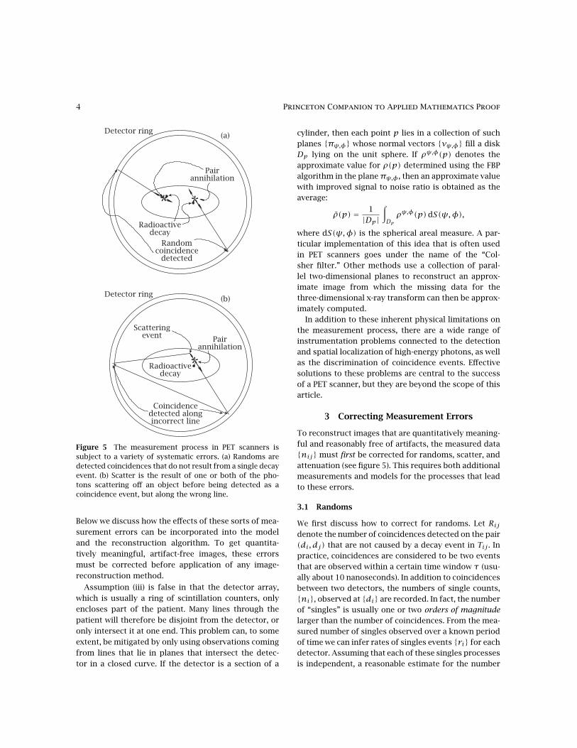
Figure 2 A radioactive decay leading to a positron–electronannihilation, exiting along �PQ , which is detected as acoincidence event at P and Q in the detector ring.

Assume, for the moment, that

(i) there are many decay events, so that we are justi-fied in replacing this probabilistic law by its mean,ρ(p),

(ii) the high-energy photons simply exit the patientwithout interaction, and

(iii) we are equally likely to detect a given decay eventon any line passing through the source point.

Let �PQ be the line joining the two detector positionsP and Q where photons are simultaneously detected.With these assumptions we see that by counting up thecoincidences observed at P and Q we are finding anapproximation to the line integral

Xρ(�PQ ) =∫�PQ

ρ(p)dl,

here dl is the arc length along the line �PQ . This is noth-ing other than a sample of the three-dimensional x-ray

sθ θs,

Figure 3 The lines in the plane π0 are labeled by θ, theangle the normal makes with the x-axis, and s, the distancefrom the line to the origin.

transform of ρ, which, if it could be approximately mea-sured with sufficient accuracy, for a sufficiently denseset of lines, could then be inverted to produce a goodapproximate value for ρ. This is essentially what isdone in x-ray ct [??].

For the moment, we restrict our attention to lines thatlie in a plane π0 intersecting the patient and choosecoordinates (x,y, z) so that π0 = {z = z0}. The linesin this plane are parametrized by an angle θ ∈ [0, π]and a real number s, with

�θ,s = {(s cosθ, s sinθ, z0)+ t(− sinθ, cosθ,0) :

t ∈ (−∞,∞)}(see figure 3). In terms of s and θ, the two-dimensionalx-ray transform is given by the integral

Xρ(s, θ, z0) =∫∞−∞ρ((s cosθ, s sinθ, z0)

+ t(− sinθ, cosθ,0))dt.

The inverse of this transform is usually representedas a composition of two operations: a filter acting onXρ(s, θ, z0) in the s variable, followed by the back-projection operator. If g(s, θ) is a function on the space

Princeton Companion to Applied Mathematics Proof 3

of lines in a plane, then the filter operation can be rep-

resented by Fg(s, θ) = ∂sHg(s, θ), where H is a con-

stant multiple of the Hilbert transform acting in the svariable. The back-projection operator X∗g defines a

function of (x,y) ∈ π0 that is the average of g over all

lines passing through (x,y):

X∗g(x,y) = 1π

∫ π0g(x cosθ +y sinθ,θ)dθ.

Putting together the pieces we get the filtered back-

projection (FBP) operator, which inverts the two-

dimensional x-ray transform: ρ(x,y, z0) = [X∗ ◦ F] ·Xρ. By using this approach for a collection of parallel

planes, the function ρ could be reconstructed in a vol-

ume. This provides a possible method for reconstruc-

tion of PET images, and indeed the discrete implemen-

tations of this method have been extensively studied. In

the early days of PET imaging this approach was widely

used, and it remains in use today. Note, however, that

using only data from lines lying in a set of parallel

planes is very wasteful and leads to images with low

signal to noise ratio.

Assumption (i) implies that our measurement is

a good approximation to the x-ray transform of ρ,

Xρ(s, θ, z0). Because of the very high energies involved

in positron emission radioactivity, only very small

amounts of short-lived isotopes can be used. The mea-

sured count rates are therefore low, which leads to mea-

surements dominated by Poisson noise that are not a

good approximation to the mean. Because the FBP algo-

rithm involves a derivative in s, the data must be signif-

icantly smoothed before this approach to image recon-

struction can be applied. This produces low-resolution

images that contain a variety of artifacts due to system-

atic measurement errors, which we describe below.

At this point it is useful to have a more accurate

description of the scanner and the measured data. We

model the detector as a cylindrical ring surrounding

the patient, which is partitioned into a finite set of

regions {d1, . . . , dn}. The scanner can localize a scintil-

lation event as having occurred in one of these regions,

which we heretofore refer to as detectors. This instru-

ment design suggests that we divide the volume inside

the detector ring into a collection of tubes, {Tij}, with

each tube defined as the union of lines joining points in

di to points in dj (see figure 4). A measurement nij is

the number of coincidence events observed by the pair

of detectors (di, dj). The simplest interpretation of nijis as a sample of a Poisson random variable with mean

Detector ring

di

dj

Tij

b2

b1

b1

Figure 4 The detector ring is divided into finitely manydetectors of finite size. Each pair (di, dj) defines a tube Tijin the region occupied by the patient. This region is dividedinto boxes {bk}.

proportional to∫�PQ⊂Tij

Xρ(�PQ ). (4)

Below we will see that this interpretation requires

several adjustments.

Assumption (ii) fails as the photons tend to interact

quite a lot with the bulk of the patient’s body. Large

fractions of the photons are absorbed, or scattered,

with each member of an annihilation pair meeting its

fate independently of the other. This leads to three

distinct types of measurement errors.

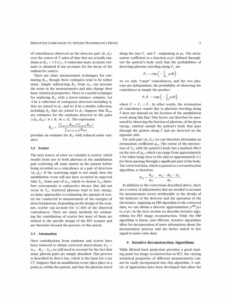
Randoms. These are coincidences that are observed by

a pair of detectors but that do not correspond to a

single annihilation event. These can account for 10–

30% of the observed events (see figure 5(a)).

Scatter. If one or both photons is/are scattered and

then both are detected, this may register as a coin-

cidence at a pair of detectors (di, dj), but the anni-

hilation event did not occur at a point lying near Tij(see figure 5(b)).

Attenuation. Most photon pairs (often 95%) are simply

absorbed, leading to a substantial underestimate of

the number of events occurring along a given line.

4 Princeton Companion to Applied Mathematics Proof

Randomcoincidence

detected

*

Pairannihilation

Radioactivedecay

Detector ring

*

*

Scatteringevent

Detector ring

(a)

(b)

Pairannihilation

Radioactivedecay

Coincidencedetected alongincorrect line

Figure 5 The measurement process in PET scanners issubject to a variety of systematic errors. (a) Randoms aredetected coincidences that do not result from a single decayevent. (b) Scatter is the result of one or both of the pho-tons scattering off an object before being detected as acoincidence event, but along the wrong line.

Below we discuss how the effects of these sorts of mea-surement errors can be incorporated into the modeland the reconstruction algorithm. To get quantita-tively meaningful, artifact-free images, these errorsmust be corrected before application of any image-reconstruction method.

Assumption (iii) is false in that the detector array,which is usually a ring of scintillation counters, onlyencloses part of the patient. Many lines through thepatient will therefore be disjoint from the detector, oronly intersect it at one end. This problem can, to someextent, be mitigated by only using observations comingfrom lines that lie in planes that intersect the detec-tor in a closed curve. If the detector is a section of a

cylinder, then each point p lies in a collection of suchplanes {πψ,φ} whose normal vectors {νψ,φ} fill a diskDp lying on the unit sphere. If ρψ,φ(p) denotes theapproximate value for ρ(p) determined using the FBPalgorithm in the planeπψ,φ, then an approximate valuewith improved signal to noise ratio is obtained as theaverage:

ρ(p) = 1|Dp|

∫Dpρψ,φ(p)dS(ψ,φ),

where dS(ψ,φ) is the spherical areal measure. A par-ticular implementation of this idea that is often usedin PET scanners goes under the name of the “Col-sher filter.” Other methods use a collection of paral-lel two-dimensional planes to reconstruct an approx-imate image from which the missing data for thethree-dimensional x-ray transform can then be approx-imately computed.

In addition to these inherent physical limitations onthe measurement process, there are a wide range ofinstrumentation problems connected to the detectionand spatial localization of high-energy photons, as wellas the discrimination of coincidence events. Effectivesolutions to these problems are central to the successof a PET scanner, but they are beyond the scope of thisarticle.

3 Correcting Measurement Errors

To reconstruct images that are quantitatively meaning-ful and reasonably free of artifacts, the measured data{nij} must first be corrected for randoms, scatter, andattenuation (see figure 5). This requires both additionalmeasurements and models for the processes that leadto these errors.

3.1 Randoms

We first discuss how to correct for randoms. Let Rijdenote the number of coincidences detected on the pair(di, dj) that are not caused by a decay event in Tij . Inpractice, coincidences are considered to be two eventsthat are observed within a certain time window τ (usu-ally about 10 nanoseconds). In addition to coincidencesbetween two detectors, the numbers of single counts,{ni}, observed at {di} are recorded. In fact, the numberof “singles” is usually one or two orders of magnitudelarger than the number of coincidences. From the mea-sured number of singles observed over a known periodof time we can infer rates of singles events {ri} for eachdetector. Assuming that each of these singles processesis independent, a reasonable estimate for the number

Princeton Companion to Applied Mathematics Proof 5

of coincidences observed on the detector pair (di, dj)over the course of T units of time that are actually ran-doms is Rij � τTrirj . A somewhat more accurate esti-mate is obtained if one accounts for the decay of theradioactive source.

There are other measurement techniques for esti-mating Rij , though these estimates tend to be rathernoisy. Simply subtracting Rij from nij can increasethe noise in the measurements and also change theirbasic statistical properties. There is a useful techniquefor replacing Rij with a lower-variance estimate. LetA be a collection of contiguous detectors including dithat are joined to dj , and let B be a similar collection,including dj , that are joined to di. Suppose that Rmnare estimates for the randoms detected in the pairs{(dn,dm) : n ∈ B, m ∈ A}. The expression

Rij =[∑m∈A Rim][

∑n∈B Rnj]∑

m∈A,n∈B Rmnprovides an estimate for Rij with reduced noise vari-ance.

3.2 Scatter

The next source of error we consider is scatter, whichresults from one or both photons in the annihilationpair scattering off some matter in the patient beforebeing recorded as a coincidence at a pair of detectors(di, dj). If the scattering angle is not small, then theannihilation event will not have occurred in expectedtube Tij . Some part of nij , which we denote Sij , there-fore corresponds to radioactive decays that did notoccur in Tij . Scattered photons tend to lose energy,so many approaches to estimating the amount of scat-ter are connected to measurement of the energies ofdetected photons. Depending on the design of the scan-ner, scatter can account for 15–40% of the observedcoincidences. There are many methods for estimat-ing the contribution of scatter but most of them arerelated to the specific design of the PET scanner andare therefore beyond the purview of this article.

3.3 Attenuation

Once contributions from randoms and scatter havebeen removed to obtain corrected observations nij =nij −Rij −Sij , we still need to account for the fact thatmany photon pairs are simply absorbed. This processis described by Beer’s law, which is the basis for x-rayCT. Suppose that an annihilation event takes place at apoint p0 within the patient, and that the photons travel

along the rays �+ and �− originating at p0. The atten-uation coefficient is a function μ(p) defined through-out the patient’s body such that the probabilities ofdetecting photons traveling along �± are

P± = exp(−∫�±μ dl

).

As we only “count” coincidences, and the two pho-tons are independent, the probability of observing thecoincidence is simply the product

P+P− = exp(−∫�μ dl

),

where � = �+ ∪ �−. In other words, the attenuationof coincidence counts due to photons traveling along� does not depend on the location of the annihilationevent along this line! This factor can therefore be mea-sured by observing the fraction of photons, of the givenenergy, emitted outside the patient’s body that passthrough the patient along � and are detected on theopposite side.

For each pair (di, dj) we can therefore determine anattenuation coefficient qij . The extent of the intersec-tion of Tij with the patient’s body has a marked effecton the size of qij , which can range from approximately1 for tubes lying close to the skin to approximately 0.1for those passing through a significant part of the body.The corrected data, which is passed to a reconstructionalgorithm, is therefore

Nij =nijqij

= nij − Rij − Sijqij

.

In addition to the corrections described above, thereare a variety of adjustments that are needed to accountfor measurement errors attributable to the details ofthe behavior of the detector and the operation of theelectronics. Applying an FBP algorithm to the correcteddata, we can obtain a discrete approximation ρFBP(p)to ρ(p). In the next section we describe iterative algo-rithms for PET image reconstruction. While the FBPalgorithm is linear, and efficient, iterative algorithmsallow for incorporation of more information about themeasurement process and are better suited to lowsignal to noise ratio data.

4 Iterative Reconstruction Algorithms

While filtered back projection provides a good start-ing point for image reconstruction in PET, the varyingstatistical properties of different measurements can-not be easily incorporated into this algorithm. A vari-ety of approaches have been developed that allow for

6 Princeton Companion to Applied Mathematics Proof

the exploitation of such information. To describe these

algorithms we need to provide a discrete measurement

model that is somewhat different from that discussed

above. The underlying idea is that we are developing a

statistical estimator for the strengths of the Poisson

processes that produce the observed measurements.

Note that these measurements must still be corrected

as described in the previous section.

In the previous discussion we described the region,

H, occupied by the patient as a continuum, with ρ(p)the strength of the radioactive decay processes, a con-

tinuous function of a continuous variable p ∈ H. We

now divide the measurement volume into a finite col-

lection of boxes, {b1, . . . , bB}. The radioactive decay of

the tracer in box bk is modeled as a Poisson process

of strength λk. For each point p ∈ H and each detec-

tor pair (di, dj), we let c(p; i, j) denote the probability

that a decay event at p is detected as a coincidence in

this detector pair. The patient’s body will produce scat-

ter and attenuation that will in turn alter the values

of c(p; i, j) from what they would be in its absence,

i.e., the area fraction of a small sphere centered at pintercepted by lines joining points in di to points in dj .

In the simplest case, the measurements {nij} would

be interpreted as samples of Poisson random variables

with meansB∑k=1

p(k; i, j)λk,

where

p(k; i, j) = 1V(bk)

∫bkc(p; i, j)dp

is the probability that a decay event in bk is detected

in the pair (di, dj). Here, V(bk) is the volume of bk.Assuming that the attenuation coefficient does not vary

rapidly within the tube Tij , we can incorporate attenu-

ation into this model, as above, by replacing p(k; i, j)with p(k; i, j) → qijp(k; i, j) = pa(k; i, j). Ignoring

scatter and randoms, the expected value of nij would

then satisfy

E[nij] =B∑k=1

pa(k; i, j)λk = nij .

In this model, scatter and randoms are regarded as

independent Poisson processes, with means λs(i, j)and λr(i, j), respectively. Including these effects, we see

that the measurement nij is then a sample of a Poisson

random variable with mean nij +λs(i, j)+λr(i, j). The

reconstruction problem is then to infer estimates for

the intensities of the sources {λk} from the observa-tions {nij}. There are a variety of approaches to solvingthis problem.

First we consider the reconstruction problem ignor-ing the contributions of scatter and randoms. The mea-surement model suggests that we look for a solution,(λ∗1 , . . . , λ

∗B ), to the system of equations

nij =B∑k=1

pa(k; i, j)λ∗k .

If the array of detectors is three dimensional, there arelikely to be many more detector pairs than boxes in thevolume. The number of such pairs is quadratic in thenumber of detectors. This system of equations is there-fore highly overdetermined, so a least-squares solutionis a reasonable choice. That is, λ∗ could be defined as

λ∗ = arg min{y : 0�yk}

∑i,j

(nij −

B∑k=1

pa(k; i, j)yk)2

.

Note that we constrain the variables {yk} to be non-negative, as this is certainly true of the actual intensi-ties. The least-squares solution can be interpreted as amaximum-likelihood (ML) estimate for λ, when the like-lihood of observing n given the intensities y is givenby the product of Gaussians:

Lg(y) =∏i,j

exp[−(nij −

B∑k=1

pa(k; i, j)yk)2 ].

It is assumed that the various observations are samplesof independent processes. If we have estimates for thevariances {σij} of these measurements, then we couldinstead consider a weighted least-squares solution andlook for

λ∗g,σ = arg min{y : 0�yk}

∑i,j

1σij

(nij −

B∑k=1

pa(k; i, j)yk)2

.

Because the data tends to be very noisy, in addi-tion to the “data term” many algorithms include aregularization term, such as

R(y) =B∑k=1

∑k∈N(k)

|yk −yk′ |2,

where for each k, the N(k) are the indices of the boxescontiguous to bk. The β-regularized solution is thendefined as

λ∗g,σ ,β = arg min{y : 0�yk}

[∑i,j

1σij

(nij −

B∑k=1

pa(k; i, j)yk)2

+ βR(y)].

Princeton Companion to Applied Mathematics Proof 7

As noted above, these tend to be very large systems ofequations and are therefore usually solved via iterativemethods. Indeed, a great deal of the research effort inPET is connected with finding data structures and algo-rithms to enable solution of such optimization prob-lems in a way that is fast enough and stable enough forreal-time imaging applications.

Given the nature of radioactive decay it is perhapsmore reasonable to consider an expression for thelikelihood in terms of Poisson processes. With

μ(i, j)(y) =B∑kpa(k; i, j)yk,

we get the Poisson likelihood function

Lp(y) =∏i,j

e−μ(i,j)(y)[μ(i, j)(y)]nijnij !

.

The expectation—maximization (EM) algorithm pro-vides a means to iteratively find the nonnegative vectorthat maximizes logLp(y). After choosing a nonnega-tive starting vector y(0), the map from y(m) to y(m+1)

is given by the formula

y(m+1)k = y(m)k

1∑i,j pa(k; i, j)

∑i,j

[ pa(k; i, j)nij∑k pa(k; i, j)y(m)k

].

(5)This algorithm has several desirable features. Firstly,if the initial guess y(0) is positive, then the positiv-ity condition on the components of y(m) is automatic.Secondly, before convergence, the likelihood is mono-tonically increasing; that is, L(y(m)) < L(y(m+1)).Note that if nij = ∑

k pa(k; i, j)y(m)k for all (i, j),then y(m+1) = y(m). The algorithm defined in (5)converges too slowly to be practical in clinical appli-cations. There are several methods to accelerate itsconvergence, which also include regularization terms.

We conclude this discussion by explaining how toinclude estimates for the contributions of scatter andrandoms to nij in an ML reconstruction algorithm. Wesuppose that nij can be decomposed as a sum of threeterms:

nij =B∑k=1

pa(k; i, j)λk + Rij + Sij. (6)

With this decomposition, it is clear how to modify theupdate rule in (5):

y(m+1)k = y(m)k

1∑i,j pa(k; i, j)

×∑i,j

[ pa(k; i, j)nij∑k pa(k; i, j)y(m)k + Rij + Sij

].

(a) (b)

Figure 6 Two reconstructions from the same PET data illus-trating the superior noise and artifact suppression attain-able using iterative algorithms: (a) image reconstructedusing the FBP algorithm and (b) image reconstructed usingan iterative ML algorithm. Images courtesy of Dr. Joel Karp,Hospital of the University of Pennsylvania.

In addition to the ML-based algorithms, there are many

other iterative approaches to solving these optimiza-

tion problems that go under the general rubric of

“algebraic reconstruction techniques,” or ART. Figure 6

shows two reconstructions of a PET image: part (a) is

the result of using the FBP algorithm, while part (b)

shows the output of an iterative ML–EM algorithm.

5 Outlook

PET imaging provides a method for directly visualiz-

ing and spatially localizing metabolic processes. As is

clear from our discussion, the physics involved in inter-

preting the measurements and designing detectors is

rather complicated. In this article we have only touched

on some of the basic ideas used to model the mea-

surements and develop reconstruction algorithms. The

FBP algorithm gives the most direct method for recon-

structing images, but the images tend to have low res-

olution, streaking artifacts, and noise. One can eas-

ily incorporate much more of the physics into itera-

tive techniques based on probabilistic models, and this

should lead to much better images. Because of the large

number of detector pairs for three-dimensional vol-

umes, naive implementations of iterative algorithms

require vast computational resources. At the time of

writing, both reconstruction techniques and the modal-

ity as a whole are rapidly evolving in response to the

development of better detectors and faster computers,

and because of increased storage capabilities.

8 Princeton Companion to Applied Mathematics Proof

Further Reading

A comprehensive overview of PET is given in Baileyet al. (2005). A review article on instrumentation andclinical applications is Muehllehner and Karp (2006).An early article on three-dimensional reconstruction isColsher (1980). An early paper on the use of ML algo-rithms in PET is Vardi et al. (1985). Review articles onreconstruction methods from projections and recon-struction methods in PET are Lewitt and Matej (2003)and Reader and Zaidi (2007), respectively.

Bailey, D. L., D. W. Townsend, P. E. Valk, and M. N.Maisey, eds. 2005. Positron Emission Tomography. Lon-don: Springer.

Colsher, J. G. 1980. Fully three-dimensional positron emis-sion tomography. Physics in Medicine and Biology 25:103–15.

Lewitt, R. M., and S. Matej. 2003. Overview of methods forimage reconstruction from projections in emission com-puted tomography. Proceedings of the IEEE 91:1588–611.

Muehllehner, G., and J. Karp. 2006. Positron emissiontomography. Physics in Medicine and Biology 51:R117–37.

Reader, A. J., and H. Zaidi. 2007. Advances in PET imagereconstruction. PET Clinics 2:173–90.

Vardi, Y., L. A. Shepp, and L. Kaufman. 1985. A statisticalmodel for positron emission tomography. Journal of theAmerican Statistical Association 80:8–20.