MEDITERRANEAN ACTION PLAN - SedNet | European …sednet.org/download/wg-282-inf-5-rev-1.pdf ·...

UNEP(DEC)/MED WG.282/Inf.5/Rev.1 22 March 2006

ENGLISH

MEDITERRANEAN ACTION PLAN

Review Meeting of MED POL - Phase III Monitoring Activities

Palermo (Sicily), Italy 12-15 December, 2005

METHODS FOR SEDIMENT SAMPLING AND ANALYSIS

UNEP/MAP

Athens, 2006

1

Table of contents: Page: I Introduction 1 II General Matters 1 A) Monitoring objectives 1 B) Definitions of hot spots 2

III Sampling Design 2 A) Objectives 2

B) Choice of sampling sites 2 C) Sampling stations 3 D) Number of samples 4 E) Sampling layer 4 F) Sampling frequency 4 IV Sampling instruments and sample handling 4 A) Sampling instruments 4 a) Grab sampler 5 b) Corer 5 c) Box Corer 7 B) Sample handling 8 a) Part of sample taken for analysis 9 b) Pre-treatment of the sample 10 Freeze-drying 10 Sieving 11 Wet sieving 12 Archiving 12 V Normalization factors 12 A) Grain size distribution 14 B) Total Inorganic Carbon (TIC) and Total 16 Organic Carbon (TOC) C) Al and/or Li 17 VI Analytical Techniques for Organic analysis 17

A) Chlorinated pesticides and PCBs 18 B) Petroleum hydrocarbons 18 C) Organo-Phosphorus pesticides 18 VII Analytical techniques for Trace Metals 18 VIII References 18 IX Conclusion 19 X Annex 22

UNEP(DEC)/MED WG.282/Inf.5/Rev.1 Page 1

I Introduction Within the Regional Seas Program of UNEP, many scientists are concerned about sediment sampling and analysis and therefore there is an increasing demand for the reliable analysis of both organic and inorganic pollutants in sediments. On the other hand, the sampling strategy set prior to the monitoring activity is critically important and should be established with caution in order to represent the sampling site and achieve the statistical objectives of a trend monitoring programme. The need for a revision of the trend monitoring programme in sediments was raised during the Second Review Meeting of MEDPOL Phase III Monitoring Activities (Saronida, 2003), after a first examination of the sediment monitoring data was made by an expert, and it was recommended by the meeting to revise the existing strategy (UNEP(DEC)/MED WG.243/4). Afterwards, an expert meeting to revise the strategy for trend monitoring of pollutants in coastal water sediments was organized in April 2005 (Athens) and the meeting report (UNEP(DEC)/MED WG.273/2) considered important recommendations for the revision. This manual aimed at presenting the state-of-the-art in sediment monitoring in coastal waters was drafted by Dr Jean-Pierre Villeneuve (IAEA/MESL). It fully took into account the recommendations of the expert meeting on both sampling strategy and analysis. A detailed section on sampling instruments and sample handling was also included in the manual, because it was observed in the training courses organized by MED POL and IAEA/MEL that there is lack of knowledge on different sampling instruments and the sampling/sample pretreatment techniques. The draft manual was discussed in the Third Review Meeting of MEDPOL Phase III Monitoring Activities (Palermo, 2005) and further comments of the meeting were incorporated in the present text. It is a considerable demand on resources to sample and analyze sediments, so, in order to facilitate the work of the laboratories in charge of the monitoring, two different approaches (see the Conclusion) are indicated for sampling, sieving and analyzing the samples: the minimum requirement and the state-of-the-art, then laboratories could use the way that would correspond better to their needs and to their budgets. II General matters Sediments have an important role in the monitoring of the environment as they are considered as the final sink of most contaminants. Marine sediments are closely inter-related to other compartments of the environment. Therefore, their use in monitoring should be part of an integrated monitoring program. A) Monitoring objectives Two basic types of monitoring are identified within the framework of MEDPOL: compliance and trend monitoring. Surveys will also be carried out in order to complement the monitoring data and facilitate decision-making for management purposes. Compliance monitoring is defined as the collection of data through surveillance programs to verify that the regulatory conditions for a given activity are being met. Trend monitoring is defined as repeated measurements of concentrations or effects over a period of time to detect possible changes with time and also with space. Sediment monitoring is usually handled within trend monitoring activities being an integral part of the monitoring system established for hot spots and coastal waters.


B) Definitions of hot spots Hot spots areas are defined by MEDPOL as being: “Point sources on the coast which potentially affect human health, ecosystems, biodiversity, sustainability or the economy in a significant manner. They are the main points where high levels of pollution loads originating from domestic or industrial sources are being discharged”.

“Defined coastal areas where the coastal marine environment is subject to pollution from one or more point or diffuse sources on the coast which potentially affect human health in a significant manner, ecosystems, biodiversity, sustainability or the economy”. III Sampling Design

A) Objectives By far the most important step in designing of the sampling strategy of the monitoring programmes is the strict definition of the objectives of the programme concerned where the objectives should be put as detailed, specific and quantifiable as possible. To do that, a number of important factors should be taken into account, including the nature of the control measure, the contaminant concerned, the nature and location of the inputs, statistical aspects of sampling and analysis etc. Regarding the statistical objectives of a trend monitoring programme:

The monitoring has to permit a statistical comparison of the concentration of contaminants between sites (spatial distribution), highlighting areas with high concentrations of contaminants that are of concern.

It is anticipated that a temporal trend monitoring programme for trace metals will at minimum have 90% power to detect a 5% per year change over a period of between 15 and 20 years. B) Choice of sampling sites

Within MED POL monitoring programmes basically two site typologies are considered: Hot spots and coastal waters. As a matter of definition, coastal zone trend monitoring is done through a network of selected fixed coastal stations, with parameters that contribute to the assessment of trends and the overall quality status of the Mediterranean Sea. This type of monitoring is carried out on a regional basis. Trend monitoring of “hot spot” areas is done at intensively polluted areas and high risk areas where control measures have to be taken. These areas are designated by local authorities according to some common definitions provided by WHO-MED POL.

Concerning sediment trend monitoring definition of hot spots and coastal areas might be stated more specifically as

- Hotspots are the most polluted sites as recorded with sediments (not necessarily always be the same with identified MED POL hot spots) and all such sites should also be monitored

- Coastal sites are sites mainly located in the near shore coastal waters and a limited representative stations should be selected for state assessments

Both hotspot and coastal areas are suitable for monitoring contaminants content in sediments, however, only sedimentary basins with positive accumulation can be considered for


monitoring. Basins having sedimentation rates >1cm/year might be favourable monitoring sites. Sensitive areas for biological life and protected areas within the near shore coastal waters are also recommended to be included in the monitoring network C) Sampling stations

Sample sites are normally chosen on a broad grid network or transects. At least three stations are recommended to be chosen along the sediment distribution gradient of a selected site to include hot spot and the near-shore coastal area. While doing so, nearby sensitive areas for biological life should also be included in the network.

In an example case, ”O” marks sampling stations in the grid below and “hot spot” station is marked by “∆”. The arrow is pointing in the direction of the residual current (distances are indicated in nautical miles). It could be recommended to limit the number of stations for data quality assurance purpose, however, the selected station(s) should be representative for the hot spot and the other area of interest.

It is also recommended to examine the selected site for sedimentary purposes as an initial step of the work in order to identify the sediment structure of the whole area as well as the sedimentation rates. Fine and regular sedimentation sites are experienced as more favourable for monitoring purposes.


D) Number of samples Multiple samples have to be collected at each station in order to achieve the statistical

sensitivity of sampling. It was recommended to take at least three samples at each station area (ex: for an area with app. 10 m depth and 10 m radius). In the pilot phase of the programme (first five years) five samples for each station is recommended to better understand the sampling variability if it is not known from previous monitoring efforts. Pooling of individual samples is not recommended especially in the pilot phase in order to achieve the field variability, which is an essential parameter for power analysis and trend tests.

E) Sampling layer

For a spatial trend monitoring at a distribution gradient, surface sediments (uppermost 1 cm) should be sampled both at hot spots and near-shore waters.

For temporal trends, it is recommended the sampling of the upper 1 cm at hot spot stations whereas at coastal near-shore sediments deeper layers could be used. However, this will depend on the specific situations.

F) Sampling frequency

As a basis and general rule, it was recommended that the sampling frequency had to be adapted considering the sedimentation rate.

It is generally accepted that for monitoring temporal trends at hotspot stations with high sedimentation rates (>1 cm/y), the sampling frequency can be initially set to yearly. If the sedimentation conditions are very variable at selected hot spots other frequencies could be adapted (in some coastal areas the sedimentation rate is on the order of 1 cm/year, taking into account the compacting of the particles and the bioturbation of the layer, this first centimetre will integrate many years of deposition, so, the frequency of sampling could be on the order of 5 years or even more). If sampling of deeper layers at near-shore coastal waters was adopted for temporal trends then sampling frequency could also be reduced according to the accumulation rate at the site. Sampling frequency is also reduced when parameters are close or below the quality targets.

IV Sampling instruments and sample handling A) Sampling instruments The type of sampling equipment required for sediment surveys is dependent upon the contaminants of interest and on the information requested. Samples of surface sediment taken from a grab can be used to provide an assessment of the present levels of contamination in an area. The use of a more sophisticated sampler, such as a box-corer, would add reliability to the sample, but also would increase the operating cost of the survey. The type of sampler should be chosen among the followings: Sediment samplers could be divided roughly into 2 different techniques: grab sampling which collects surface and near surface sediments and coring which collects a column of the subsurface sediment and could be required to establish the historical pattern of the


contamination. In all grab and core operations, a slow approach to the sea floor should be ensured to avoid the creation of “bow wave” that disturbs the sediment-water interface prior to sampling. In some circumstances, it would be, also, possible to have the samples collected by divers using either glass or Teflon beakers. a) Grab sampler Undisturbed surface sediment samples can provide an immediate assessment of the present levels of contamination in the area in relation to the textural and geo-chemical characteristics of the sediment. The sampler used must consistently collect relatively undisturbed samples to a required depth below the sediment surface and of sufficient volume to permit subsequent analyses. The Van Veen grab is among the most commonly used grab samplers. With this bottom sampler, samples can be extracted from any desired depth. While it is being lowered, both levers are locked wide apart whereby the jaws are open. Upon making contact with the waterbed, the locking mechanism is released and when the rope is pulled out to raise the sampler, the jaws close. The small model (Figure 1), with a surface of 250 cm2, made of stainless steel has a weight of approximately 5 kg and could be hand-operated from a small vessel. It is not recommended for greater water depth. The main problem with this sampler is that it is sometimes difficult to recover the surface layer of the sediment, so this type of sampler could be used only in case a coring device is not available.

Figure 1: Van Veen grab operated manually (picture from Hydro-Bios, Germany). There are other models of Van Veen grab, which are winch-operated, with a weight up to 80 kg. These models are represented in annex. b) Corer Sediment subsurface samples are often taken using barrel or box corers to determine the change in lithology and chemical composition with depth in order to assess environmental changes in metal fluxes with time. Cores are usually collected in areas of fine-grained sediments but specialized corers are available for coarse-grained sediments.


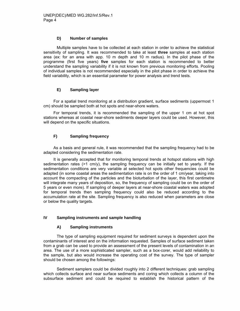
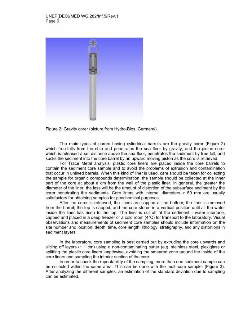
Figure 2: Gravity corer (picture from Hydro-Bios, Germany). The main types of corers having cylindrical barrels are the gravity corer (Figure 2) which free-falls from the ship and penetrates the sea floor by gravity, and the piston corer which is released a set distance above the sea floor, penetrates the sediment by free fall, and sucks the sediment into the core barrel by an upward moving piston as the core is retrieved. For Trace Metal analysis, plastic core liners are placed inside the core barrels to contain the sediment core sample and to avoid the problems of extrusion and contamination that occur in unlined barrels. When this kind of liner is used, care should be taken for collecting the sample for organic compounds determination, the sample should be collected at the inner part of the core at about a cm from the wall of the plastic liner. In general, the greater the diameter of the liner, the less will be the amount of distortion of the subsurface sediment by the corer penetrating the sediments. Core liners with internal diameters > 50 mm are usually satisfactory for obtaining samples for geochemical purposes. After the corer is retrieved, the liners are capped at the bottom; the liner is removed from the barrel; the top is capped, and the core stored in a vertical position until all the water inside the liner has risen to the top. The liner is cut off at the sediment - water interface, capped and placed in a deep freezer or a cold room (4°C) for transport to the laboratory. Visual observations and measurements of sediment core samples should include information on the site number and location, depth, time, core length, lithology, stratigraphy, and any distortions in sediment layers.

In the laboratory, core sampling is best carried out by extruding the core upwards and slicing off layers (~ 1 cm) using a non-contaminating cutter (e.g. stainless steel, plexiglass or splitting the plastic core liners lengthwise, avoiding the smeared zone around the inside of the core liners and sampling the interior section of the core. In order to check the repeatability of the sampling, more than one sediment sample can be collected within the same area. This can be done with the multi-core sampler (Figure 3). After analyzing the different samples, an estimation of the standard deviation due to sampling can be estimated.


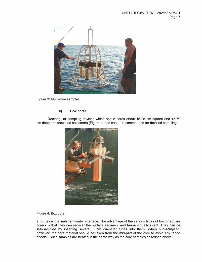
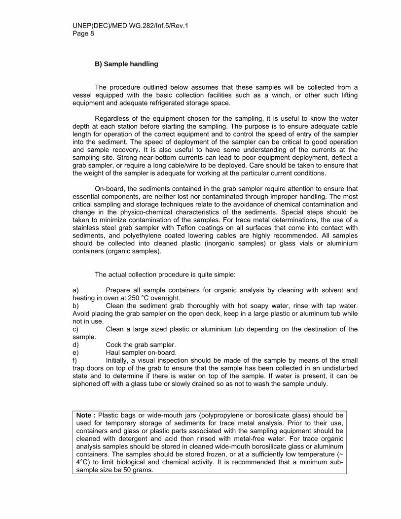
Figure 3: Multi-core sampler. c) Box corer Rectangular sampling devices which obtain cores about 15-25 cm square and 15-60 cm deep are known as box corers (Figure 4) and can be recommended for detailed sampling Figure 4: Box corer. at or below the sediment-water interface. The advantage of the various types of box or square corers is that they can recover the surface sediment and fauna virtually intact. They can be sub-sampled by inserting several 5 cm diameter tubes into them. When sub-sampling, however, the core material should be taken from the mid-part of the core to avoid any “edge effects”. Such samples are treated in the same way as the core samples described above.


B) Sample handling The procedure outlined below assumes that these samples will be collected from a vessel equipped with the basic collection facilities such as a winch, or other such lifting equipment and adequate refrigerated storage space. Regardless of the equipment chosen for the sampling, it is useful to know the water depth at each station before starting the sampling. The purpose is to ensure adequate cable length for operation of the correct equipment and to control the speed of entry of the sampler into the sediment. The speed of deployment of the sampler can be critical to good operation and sample recovery. It is also useful to have some understanding of the currents at the sampling site. Strong near-bottom currents can lead to poor equipment deployment, deflect a grab sampler, or require a long cable/wire to be deployed. Care should be taken to ensure that the weight of the sampler is adequate for working at the particular current conditions. On-board, the sediments contained in the grab sampler require attention to ensure that essential components, are neither lost nor contaminated through improper handling. The most critical sampling and storage techniques relate to the avoidance of chemical contamination and change in the physico-chemical characteristics of the sediments. Special steps should be taken to minimize contamination of the samples. For trace metal determinations, the use of a stainless steel grab sampler with Teflon coatings on all surfaces that come into contact with sediments, and polyethylene coated lowering cables are highly recommended. All samples should be collected into cleaned plastic (inorganic samples) or glass vials or aluminium containers (organic samples). The actual collection procedure is quite simple: a) Prepare all sample containers for organic analysis by cleaning with solvent and heating in oven at 250 °C overnight. b) Clean the sediment grab thoroughly with hot soapy water, rinse with tap water. Avoid placing the grab sampler on the open deck, keep in a large plastic or aluminum tub while not in use. c) Clean a large sized plastic or aluminium tub depending on the destination of the sample. d) Cock the grab sampler. e) Haul sampler on-board. f) Initially, a visual inspection should be made of the sample by means of the small trap doors on top of the grab to ensure that the sample has been collected in an undisturbed state and to determine if there is water on top of the sample. If water is present, it can be siphoned off with a glass tube or slowly drained so as not to wash the sample unduly. Note : Plastic bags or wide-mouth jars (polypropylene or borosilicate glass) should be used for temporary storage of sediments for trace metal analysis. Prior to their use, containers and glass or plastic parts associated with the sampling equipment should be cleaned with detergent and acid then rinsed with metal-free water. For trace organic analysis samples should be stored in cleaned wide-mouth borosilicate glass or aluminum containers. The samples should be stored frozen, or at a sufficiently low temperature (~ 4°C) to limit biological and chemical activity. It is recommended that a minimum sub-sample size be 50 grams.


g) Once the top of the sediment is exposed, visual estimates of grain-size (coarse, medium, fine grained), color, and the relative proportions of the components should be made and recorded. In situ measurements such as pH can be made by inserting the appropriate electrodes into the sample. h) Most fine-grained sediments usually have a thin, dark yellowish brown surface layer resulting from the oxidization of iron compounds at the sediment-water interface. Since in most cases this layer represents the material being deposited at the present time, it should be sampled carefully with a non-contaminating utensil such as a plastic spatula for trace metals determination and a stainless steel one for organic compounds determination. About 10-30 g should be placed in a numbered polyethylene vial for trace metal analysis and in glass or aluminium container for organic analysis, sealed and frozen for transport to the laboratory. i) After the surface layer has been sampled, the grab can be opened and an additional sample, representative of the subsurface, can be obtained. Observations of this material should include color and textural characteristics. To ensure a representative sample, about 100 to 200 grams (or even more) should be collected and placed in a numbered vial. The sample should be frozen quickly for return to the laboratory. Larger samples of about 1 kg are required for admixtures of gravel, sand and mud. j) Store all sediment samples deep-frozen or, at least, under refrigeration (4oC) until they are transported to the laboratory. a) Part of sample taken for analysis Depending on the analysis required and on the material of the sampler (plastic liner for corer), the collection of sediment should follow an agreed protocol. The main idea being to avoid contact with plastic liner for organic compounds and contact with stainless steel for trace elements analysis.


Figure 5: Collection of sediment according to analysis required. The distribution of sediment depending on the analysis to be performed is indicated on the Figure 5. b) Pre-treatment of the sample Freeze-drying: After collection, the sediment samples are transferred into pre-cleaned aluminium boxes or pre-cleaned aluminium paper for organic analysis or into plastic bags for trace element analysis and deep-frozen (or at least kept refrigerated at about 4°C during the transport to the laboratory in order to avoid the bacterial degradation in case of petroleum hydrocarbon analysis). When in the laboratory, the sediment samples should be deep-frozen at -20°C and, when frozen, freeze-dried in a freeze-dryer. But it is always interesting to archive part of the sample in order to be able to re-analyze it in case of suspected contamination during the analytical process. So, before freeze-drying, one half of the sample should be stored, as such,


in the deep-freezer for future reference (in this case it could be interesting to have a -80°C deep-freezer). In order to proceed with minimal risk of contamination in the freeze-dryer, the samples should be covered with aluminium paper with some pins holes to let the water vapor evacuate and reduce the eventual cross-contamination. Contamination from the freeze-dryer and from the vacuum pump should be monitored by freeze-drying, with all batch of samples, a portion of clean Florisil. By analyzing the Florisil it is, then, possible to check if the freeze-dryer does not contaminate the samples. The samples could be weighed before and after freeze-drying in order to access the ratio of dry/wet weight for each sample. Note: for frozen sample there is no storage limit in time, for freeze-dried samples, if the samples are kept in the dark, in a cool place (20°C) and with Teflon tape around the neck of the bottles to avoid the humidity to enter in the sample, the limit of conservation could be on the order of 10-15 years without deterioration of the sample. Sieving: After freeze-drying the sediment samples could be sieved in order to remove the small gravels, pieces of branches and shelves. Before sieving, it is recommended to sort out, with stainless steel forceps (for organic analysis), or with plastic ones (for trace metal analysis), in the sediment sample the small pieces of shelves, branches and leaves that could be present in the sample in order to avoid the contamination by extra materials. Then, to do that, the samples are transferred in the top sieve of a sieving machine and the machine is activated. Doing so, the sediment will be disaggregated and not crushed. The question of sieving is very delicate, as many possibilities exist. One will sieve at 1 or even 2 mm (pre-sieving), only to remove the small pieces of shelves, leaves and branches, some will sieve at 250 µm. In most cases, sieving the sediments through a 63 µm sieve in order to separate the silt and clay from the sand and coarser material is both useful and practicable and it is a widely adopted procedure (However, sieving is not recommended for fine and homogeneous sediments, usually found in the zones with high sedimentation rates where the content of the contaminants will be highest because of their wealth of fine particles for which the contaminants have a particular affinity. Obviously, when it is not possible to find fine sediments, sieving can be recommended to extract the finest particles). Ideally, sieving could be made at 63 µm and the fraction with less than 63 µm and the fraction of more than 63 µm could be analyzed. Even in some cases, sieving at 20 µm is undertaken and 3 fractions are, then, analyzed: more than 63 µm, between 20 µm and 63 µm and less than 20 µm. Since sieving may also cause contamination problems of the samples (basically for the organic contaminants), many steps of sieving should be avoided -if it could be- and it may even be recommended to sieve only from 250 µm before organic contaminant analysis.

For spatial trend monitoring sieving is not a critical issue however sieving from <1mm or <2 mm in the field could be recommended directly after sampling or after freeze-drying step.

For temporal studies sieving could be recommended over 63 µm. However, it is

important to achieve the programme consistency, therefore, if all set criteria in terms of sufficient trend detection are met by a laboratory that is using a whole fraction (e.g. less than 1 or 2 mm) for temporal studies, at present it is not recommended to switch to any other fraction.


Wet sieving: Some laboratories are using wet sieving techniques. One of the problems that occurs with this technique is the possibility of contamination for organic samples as the material used for this wet sieving method are plastic (silicone tubing and plastic tubes with nylon nets), another problem, also, has to be taken into consideration is the time spent on this wet sieving technique. This wet sieving method could be used for trace metal work and in well-equipped and staffed laboratories. Archiving: Archiving sediment (and biota) samples is a must in QA/QC procedures. All samples should be kept for the duration of the monitoring in order to be able to come back to any of them, or to all of them, in case of problems. Archives should consist of different parts: the first one being the sample wet and deep-frozen as it has been collected. This archive will be used in case of contamination that can appear during the freeze-drying process. So, one part of the original sample can be extracted again, even wet and dried with sodium sulfate, if it appears that the freeze-dryer had contaminated the sample. Then when the sample has been dried, and an aliquot has been analyzed, the remaining sediment sample should be kept in a glass bottle, with Teflon tape around the closing system (that should be aluminium for organic and plastic for trace metal) to protect against the moisture and then, stored in a cupboard in the dark and cool place. This way, the sample archived can be stored for 10-15 years, so, for the duration of the monitoring program. V Normalization factors Normalization is a process that could reduce the discrepancy between data sets by taking into account the differences in grain size distribution and in the mineralogy (sediment composition) between samples. Both trace metals and organic contaminants concentrations will co-vary with such grain size, and organic carbon content. As an example, metals and organic contaminants show a much higher affinity to fine particles than to the coarse fraction. For normalization purpose, in order to account for the metal variations in respect to the variations of the aluminosilicate mineral fraction, the determination of, at least, Al and/or Li are recommended followed by Fe and Mg. In case of temporal trend monitoring, the idea consists in making comparison with time within a series of independent locations. The critical factor will be to ensure that from one year to the other the laboratory will always analyze the same grain size fraction to be able to compare the data obtained.

It should also be stressed that normalization of the results can only berecommended if there is a strong statistical relation between the contaminantconcentration and the normalizer. In the contrary case, it can distort the interpretation ofthe results.


Summary of Normalization Factors (from UNEP/IOC/IAEA, 1995) Normal. factor Size Indicator Role Textural µm ------------------------------------------------------------------------------------------------------------------------------ Grain Size 2000-< 2 Granular variations Determines physical of metal bearing minerals/ sorting and depositional compounds patterns of metals Sand 2000-63 Coarse grained metal-poor Usually diluent of trace Minerals/compounds metal concentrations Mud < 63 Silt and clay size metal Usually overall concentrator bearing minerals/ of trace metals* compounds Clay < 2 Metal-rich clay minerals Usually fine grained Accumulator of trace Metals* Normal. factor Size Indicator Role Textural µm Chemical Si Amount and distribution of Coarse grained diluter of Metal-poor quartz trace metal concentrations Al Al silicates, but used to Chemical tracer of Al- account for granular silicates, particularly variations of metal rich the clay minerals* fine silt + clay size Al- Silicates Fe Metal-rich silt + clay Chemical tracer for Fe-rich size Fe bearing clay clay minerals minerals, Fe rich heavy minerals and hydrous Fe oxides Sc Sc structurally combined Tracer of clay minerals in clay minerals which are concentrators of trace metals Cs Cs structurally combined Tracer of clay minerals in clay minerals and which are concentrators feldspars of trace metals Li Li structurally combined Tracer of clay minerals, in clay minerals and micas particularly in sediments containing Al-silicates in all size fractions Organic Carbon Fine grained organic Sometimes accumulator of matter trace metals like Hg and Cd * except in sediments derived from glacial erosion of igneous rocks


A) Grain size distribution

The methods for fractionation into grain size can be found in UNEP/IOC/IAEA, 1995 and in Loring and Rantala, 1992. The sequence of steps for the grain size separation of sediment sample can be found in Figure 6, below.

Some instrumentation, also, is available for grain size studies (example of the

Mastersizer). Preparation prior particle size analysis: Samples are freeze-dried and sieved at 250 µm. Aliquots of about 1gram are used for particle size analysis. Approximately an aliquot of 1g of sediment was put in a 10mL tube. 5mL of MilliQ water is added and tube is shaken in order to separate properly the silt particles. A period of about half an hour is taken to assure that the sample is homogeneously wet before analysis. Introduction to Particle Size Analysis:

The Mastersizer is based on the principle of laser ensemble light scattering. It falls into the category of non-imaging systems due to the fact that sizing is accomplished without forming an image of the particle onto a detector. The Mastersizer employs two forms of optical configuration to provide its unique specification. The first is the well-known optical method, called “conventional Fourier optics”. The second is called “reverse Fourier optics”, used in order to allow the measurement size range to be extended down to 0.05µm. There are restrictions placed upon the sample presentation requirements in this configuration, which limit its availability to particles dispersed in liquid suspension.


GRAIN SIZE SEPARATION

Split to get desired sample

Add dispersant and wet sieve

<63 µm fraction

>63µm fraction

Pipette analysis

Thoroughly dry for dry sieving analysis (receiving pan –1.0∅ down 4.0∅)

Grain >2 mm (∅10)

Yes

Collected Grains <63 µm

No END

Weigh Figure 6: Sequence of steps for the grain size separation of a sediment sample

The result of the measurement analysis is a volume distribution characterized over the

size limits of the optical configuration used. The results may be presented in a number of ways to suit the users needs. For this study, the distribution is listed as a table of results, giving frequency and cumulative forms of distribution. It is also plotted on a log size axis high-resolution graph in frequency and oversize form. In addition to this treatment of the fundamental volume measurement it is possible to derive further information using numerical transformations. Finally the standard derived diameters are provided, complete with volume percentiles.


B) Total Inorganic Carbon (TIC), Total Organic Carbon (TOC) Organic material interacts strongly with both organic and inorganic contaminants. The organic carbon is one of the measures of the organic material. Another parameter would be the determination of lipids, or lipid-like material. The measurement of the hexane extractable organic matter (or HEOM) is also a normalising variable. The carbonate content (inorganic carbon) of the sediment is generally considered as a dilution factor of the main phases carrying the contaminants and should, also be determined. Total inorganic carbon (or carbonates) are obtained by the difference of data: TIC (%) = TC (%) – TOC (%) Preparation of samples: Samples for TC analysis are weighed (mg) in tin boats and directly analysed. Samples for TOC analysis are weighed (mg) in tin capsules and acidified with H2PO4 1M until the inorganic carbon is removed (3 times in 8 hours intervals to the oven at 55°C). Tin boats and capsules are folded and pressed before the analysis. Procedure: Analyses could be done with automatic analyser (such as Elementar “VARIO EL” Instrument) in CN mode. For the mass determination of C and N, an oxidation of the sample followed by the reduction of nitroxides is realized, coupled to chromatographic glass column separation and thermal conductivity detection for CO2 and N2. Note: In case a CHN analyser is available and used for the TC-TOC analysis, Total Nitrogen and Total Organic Nitrogen can be measured simultaneously which can provide a general insight of the lability of organic matter, simply based on the C/N ratio. Quality control: Acetanilide standard (C8H9NO) is used as a correction factor for accurate and precise measurements (71.1 % C and 10.4 % N) and to control instrumental stability. The precision of TOC and TC measurements in the samples depends in numerous random factors such as: weighing, use of an acidification step, sample structure (i.e. matrix), concentrations, as well as the instrumental noise. Coefficients of variation (% RSD) must be calculated for each pair of determination, specially, for TOC analysis, which includes an acidification step. Alternative method to estimate Organic Material in case a CHN Analyser is not available: The Organic Matter (OM) content in sediments can be measured with the following method: 1) Put the (wet) sediment sample in oven at 60°C for 24 hours (up to constant weight).


2) Weight approximately 1 g of dry sediment (precision 0.01 mg) in a small porcelain boat. 3) Put the sediment for ignition into a furnace at 450°C for 3 hours. 4) Weight the sediment after ignition (precision 0.01 mg). The Organic Matter (OM) content is equivalent to the percentage of Loss of Weight (LOI %) LOI % = (Wdry – Wign) x 100 / Wdry Where: LOI % = Loss on Ignition (equivalent to the total Organic Matter) Wign = Weight after ignition Wdry = Weight of dry sediment before ignition C) Al and/or Li It has been observed that in many contaminated and uncontaminated environments, the majority of the trace elements are held in the fine-grained, alumino-silicate fraction of the sediment. When the fine-grained material is uncontaminated and from the same provenance, the ratios of trace metals to conservative elements, such as aluminium or lithium, is almost constant. If provenance of the sediment remains practically constant in a studied area, this consistency should be reflected in the metal to aluminium ratios. Plots of individual metal concentrations against aluminium concentrations will be linear and significant deviations from the linear relationship would reflect a contaminated area. Loring and Rantala (1992) conclude their paper by stating that “the use of the granulometric measurements, metal/Al, metal/Li or other metal/reference element ratios are all useful approaches towards complete normalization of granular and mineralogical variations, and identification of anomalous metal concentrations in sediment”. VI Analytical Techniques for Organic analysis Before proceeding to the analysis, an aliquot will be taken from the bulk sample and in order to be sure that what is analyzed is representative of the collected sample, the sediment sample should be well homogenized. This could be done in a specialized laboratory homogeneizer, but it could be done, more simply, with a spatula, taking care of mixing well the sediment sample before collecting the 10 g aliquot (for organic) or the 1-2 g aliquot (for trace metal) for the extraction. The analytical part can be found in the Reference Methods for Marine Pollution Studies published by UNEP. All these Reference Methods are available, free of charge, from IAEA-MEL/MESL. With all set (one for 10 samples, as a minimal requirement) of sediment samples extracted, a sediment Reference Material should be extracted to check the quality of the data produced (UNEP/IOC/IAEA/FAO, 1990).


A) Chlorinated pesticides and PCBs.

For Chlorinated pesticides and PCBs in sediment samples, the analytical part can be found in UNEP/IOC/IAEA, 1996.

B) Petroleum Hydrocarbons. The analytical part for petroleum hydrocarbon analysis can be found in UNEP/IOC/IAEA, 1992. C) Organo-Phosphorus pesticides The organophosphorus analytical method of sediment samples can be found in UNEP/FAO/IOC/IAEA, 1997. VII Analytical technique for Trace Metals For trace elements, in general, the methods can be found in UNEP/IOC/IAEA, 1995. For mercury: UNEP/IAEA, 1985 and UNEP/IOC/IAEA, 1985. VIII References F. Ackerman (1980). A procedure for correcting the grain size effect in heavy metal analysis of estuarine and costal sediments. Environmental Technology Letter, 1, 518. K. Bertine (1978). Means of determining nature versus anthropogenic fluxes to estuaire sediments. In: Biochemistry of estuaire sediments. Proceeding of a UNESCO/SCOR workshop held in Melreux, Belgium, 246-253. D. Claisse, B. Boutier, J. Tronczinsky (1998). RNO Surveillance du Milieu Marin, Travaux du Reseau National d’Observation de la Qualite du Milieu Marin, IFREMER. Commission OSPAR (1999). Lignes directrices JAMP de la surveillance continue des contaminants dans les sediments. Ref. No 1999-1. Commission OSPAR (1997). Teneurs ambiantes de reference convenues pour les contaminants dans l’eau de mer, le milieu vivant et les sediments. Guidelines for the use of sediments in marine monitoring in the context of Oslo and Paris commissions programmes (1993). ICES Coop. Res. Rep. No 198. International Council for the Exploration of the Sea (2000). Report of the working group on marine sediments in relation to pollution, ICES CM 2000/E: 03. Ref.: ACME. M. Kersten and F. Smedes (2002). Normalization procedures for sediment contaminants in special and temporal trend monitoring. J. Environ. Monit., 4, 109-115.


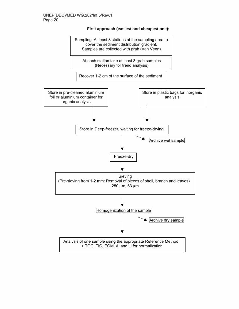
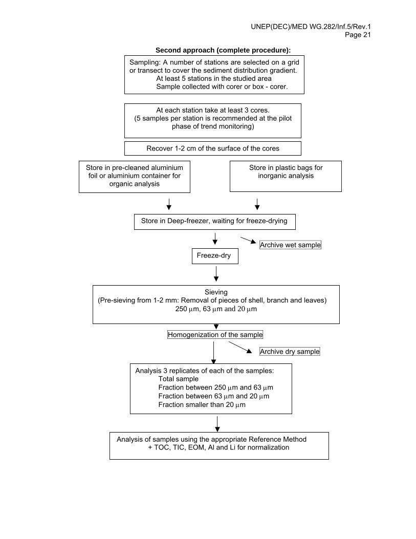
D. H. Loring and R. T. T. Rantala (1992). Manual for the geochemical analyses of marine sediments and suspended particulate matter. Earth-Science Reviews, 32, 235-283. D. H. Loring (1990). Lithium: a new approach for the granulometry normalization of trace metalsdata. Mar. Chem., 29 (2-3), 155-158. V. Roussiez, W. Ludwig, J. L. Probst and A. Monaco (2005). Background levels of heavy metals in surficial sediments of the Gulf of Lions (NW Mediterranean): An approach based on 133Cs normalization and lead isotope measurements. Environmental Pollution, 138, 167-177. F. Smedes (1997). Grainsize correction procedures. Report of the ICES Working Group on Marine Sediments in Relation to Pollution. ICES CM 1997 / Env: 4, Annexe 6. UNEP/FAO/IOC/IAEA (1997) Reference Methods for Marine Pollution Studies No “AE”. Determination of selected organophosphorus contaminants in marine sediments. UNEP, 1997. UNEP/IOC/IAEA (1996). Reference Methods for Marine Pollution Studies No 71. Sample work-up foe the analysis of selected chlorinated hydrocarbons in the marine environment. UNEP, 1996. UNEP/IOC/IAEA (1995). Reference Methods for Marine Pollution Studies No 63. Manual for the geochemical analyses of marine sediments and suspended particulate matter. UNEP, 1995. UNEP/IOC/IAEA (1992). Reference Methods for Marine Pollution Studies No 20. Determination of petroleum hydrocarbons in sediments. UNEP, 1992. UNEP/IAEA (1985). Reference Methods for Marine Pollution Studies No 26. Determination of total mercury in marine sediments and suspended solids by cold vapor atomic absorption spectrophotometry. UNEP, 1985. UNEP/IOC/IAEA (1985). Reference Methods for Marine Pollution Studies No 19. Determination of total mercury in estuarine waters and suspended sediment by cold vapor atomic absorption spectrophotometry. UNEP, 1985. UNEP/IOC/IAEA/FAO (1990). Reference Methods for Marine Pollution Studies No 57. Contaminant monitoring programmes using marine organisms: Quality Assurance and Good Laboratory Practice, UNEP, 1990. IX Conclusion We can consider two different approaches to the sediment sampling for monitoring projects. They follow the schematics below depending on the budget and the manpower of the laboratories. One of the methods is a minimum requirement and the other would be the “state-of-the-art” methodology.


First approach (easiest and cheapest one): Archive wet sample

Homogenization of the sample

Archive dry sample

Sampling: At least 3 stations at the sampling area to cover the sediment distribution gradient.

Samples are collected with grab (Van Veen)

Recover 1-2 cm of the surface of the sediment

Store in pre-cleaned aluminium foil or aluminium container for

organic analysis

Store in plastic bags for inorganicanalysis

Store in Deep-freezer, waiting for freeze-drying

Sieving (Pre-sieving from 1-2 mm: Removal of pieces of shell, branch and leaves)

250 µm, 63 µm

Analysis of one sample using the appropriate Reference Method + TOC, TIC, EOM, Al and Li for normalization

At each station take at least 3 grab samples (Necessary for trend analysis)

Freeze-dry


Second approach (complete procedure):

Archive wet sample

Homogenization of the sample Archive dry sample

Sampling: A number of stations are selected on a gridor transect to cover the sediment distribution gradient. At least 5 stations in the studied area Sample collected with corer or box - corer.

Recover 1-2 cm of the surface of the cores

Store in pre-cleaned aluminium foil or aluminium container for

organic analysis

Store in plastic bags for inorganic analysis

Store in Deep-freezer, waiting for freeze-drying

Freeze-dry

Analysis of samples using the appropriate Reference Method + TOC, TIC, EOM, Al and Li for normalization

At each station take at least 3 cores. (5 samples per station is recommended at the pilot

phase of trend monitoring)

Sieving (Pre-sieving from 1-2 mm: Removal of pieces of shell, branch and leaves)

250 µm, 63 µm and 20 µm

Analysis 3 replicates of each of the samples: Total sample Fraction between 250 µm and 63 µm Fraction between 63 µm and 20 µm Fraction smaller than 20 µm


X Annex Pictures of some sediment sampling devices.

Large grab sampler Shipeck grab sampler. (picture: S. de Mora)

Bottom sampler Ekman-Birge Gravity core sampler (picture: Hydro-Bios, Germany). (picture: S. de Mora)

Reineck corer

Date post:	21-Mar-2018
Category:	Documents
Upload:	vancong
View:	220 times
Download:	5 times

MEDITERRANEAN ACTION PLAN - SedNet | European …sednet.org/download/wg-282-inf-5-rev-1.pdf ·...

Documents