Medium Modified Perturbative QCD Calculation of Splitting Functions Liliana Marisa Cunha Apolin´ ario Disserta¸c˜ ao para a obten¸c˜ao de Grau de Mestre em Engenharia F´ ısica Tecnol´ ogica J´ uri Presidente: Professor Jo˜ ao Carlos Carvalho de S´ a Seixas Orientador: Professor Jos´ e Guilherme Teixeira de Almeida Milhano Vogais: Professor Doutor Jorge Venceslau Comprido Dias de Deus Setembro 2009
Transcript
Medium Modified Perturbative QCDCalculation of Splitting Functions
Liliana Marisa Cunha Apolinario
Dissertacao para a obtencao de Grau de Mestre em
Engenharia Fısica Tecnologica
Juri
Presidente: Professor Joao Carlos Carvalho de Sa Seixas
Orientador: Professor Jose Guilherme Teixeira de Almeida Milhano
Vogais: Professor Doutor Jorge Venceslau Comprido Dias de Deus
Setembro 2009
Acknowledgments
I would like to thank to all the people who directly or indirectly influenced the course of my workand without whom this thesis would have never been completed.
To my supervisor, Guilherme Milhano, for his patience, support and valuable help. Despite thedistance, he always arranged time to answer questions, solve problems and discuss ideas until wereno more doubts. My many thanks to him.
To Jeremy Miller, for all useful discussions and who many times help me with mathematical issues.To Jorge Casalderrey-Solana and Nestor Armesto who help me a lot with the understanding ofthe physics and calculations of Jet-Quenching. To prof. Mario Pimenta, for his kindness and forhelping me to clarify what was the next step when it seemed that there were none.
To my master colleague, Samuel Abreu, for sharing ideas for the thesis contents and useful discus-sions. To Antonio Vale, Goncalo Dias and Andrea Nerozzi for providing me some of the bibliographyand solving all the problems with the Macintosh computer.
To my friend Marta Silva, who heard most of my frustrations from my work for countless timesand for making me feel better after each conversation. To Pedro Martins for its company and allthe coffee breaks we made. To David Seixas and Ricardo Nunes, for their company during thecourse.
To Dulce Conceicao, who help me so much with the bureaucracy of IST. Without her, I wouldnever have gone to CERN. To prof. Joao Seixas, for his availability with the Bolonha process, thethesis subscription and dissertation.
Gostaria tambem de agradecer a minha famılia, pela sua preocupacao, carinho e dedicacao. Emespecial, aos meus futuros sogros que sao como uns segundos pais para mim, a minha tia Carmencitae ao meu tio Lelinho de quem eu gosto tanto, e aos meus avos, cujo espırito lutador e um exemploa seguir. O meu especial obrigada a eles.
Por ultimo, as tres pessoas mais importantes na minha vida, que me acompanharam no curso, emparticular neste ultimo ano. Durante a realizacao desta tese e de todo o trabalho aliado a ela,foram muitas as dificuldades encontradas, de todas as formas e feitios e exasperantes. Mas elesnunca me deixaram parar e sempre me ajudaram a lutar. O seu carinho e compreensao forammais que o imaginavel e devo-lhes muito do que consegui alcancar ate agora. Refiro-me ao meupai e a minha mae, que sempre fizeram tudo que estava ao seu alcance para me ajudar e que meaturaram nos momentos difıceis. A sua presenca e o seu apoio foram indispensaveis na realizacao
i
desta tese. E ao meu namorado Ruben, a pessoa que mais me acompanhou nesta tese, por se tersentado ao meu lado a resolver muitos dos problemas fısicos que tive, por ter feito as perguntasque me ajudaram a perceber onde eu tinha duvidas, por ter questionado as minhas decisoes paraencontrar uma melhor. Todo o seu carinho, amizade e amor fizeram-me forte o suficiente parasuperar as dificuldades.
E a eles que eu dedico esta tese! Muito obrigada!
ii
Resumo
O estudo de Jet-Quenching em colisoes de ioes pesados, i.e., a perca de energia e a fragmen-tacao modificada dos partoes que atravessam um meio denso, esta na linha da frente dos actuaisesforcos teoricos e experimentais. A sua compreensao em termos quantitativos e essencial parauma interpretacao dos dados de RHIC (e num futuro proximo do LHC) e para uma consequentecaracterizacao do meio produzido.
A presente tese tem como objectivo calcular as funcoes de splitting modificadas pelo meio, ondeestao incluıdos todos os efeitos inerentes a propagacao de uma partıcula altamente energeticaatraves de um meio. Para isso, no capıtulo 1, a ideia principal e dar uma visao geral da teoriaQCD, quais as suas bases, o que e que a suporta e quais as suas limitacoes. Tambem seraoabordadas outras caracterısticas mais fısicas. No capıtulo 2 veremos a propagacao e consequenteevolucao de quarks e gluoes no vacuo, bem como uma derivacao das equacoes de evolucao DGLAPe respectivas funcoes de splitting. De seguida, segue-se um estudo intensivo sobre propagacao nomeio no capıtulo 3. Aqui veremos o fenomeno de Jet-Quenching e os principais modelos usadosactualmente para o descrever. Usaremos um destes modelos para calcular o espectro de gluoesradiados na presenca de um meio e respectivas funcoes de splitting modificadas. O resultado e umtermo de correccao presente em todas as funcoes de splitting que depende da energia e do momentotransverso transportados pelo partao final. As conclusoes sao apresentadas no capıtulo 4.
Palavras-chave: QCD, DGLAP, Jet-Quenching, Funcoes de Splitting
iii
iv
Abstract
The study of Jet-Quenching in heavy ion collisions, i.e., the energy loss and modified branchingof partons transversing dense media, is at the forefront of current theoretical and experimentalefforts. Its quantitative understanding is essential for the interpretation of data from RHIC (andin a near future from the LHC) and consequent characterization of the medium produced.
This thesis aims to compute the medium-modified splitting functions, where it is included all theeffects of medium propagation done by a highly energetic particle. For doing so, in chapter 1 themain idea is to give a general perspective about the theory of QCD, what are its foundations,what supports the theory and what are its limitations. In chapter 2, we will see the propagationand consequent evolution of quarks and gluons in a vacuum, as well as a derivation of the DGLAPevolution equations and respective splitting functions. Then it follows an intensive study of mediumpropagation in chapter 3. Here we will see the phenomena of Jet-Quenching and the main modelsused nowadays to describe this phenomena. We will use one of these models to compute thespectrum of radiated gluons in a presence of a medium and respective medium-modified splittingfunctions. The results is a correction term present in all four splitting functions, that depends onthe energy and transverse momentum carried by the final parton. The conclusions are presentedin chapter 4.
1.1 Deep Inelastic Scattering (a) and Elastic Scattering (b) . . . . . . . . . . . . . . . 21.2 Deep inelastic scattering seen by the parton model . . . . . . . . . . . . . . . . . . 31.3 Test of Bjorken scaling using the e−p deep inelastic scattering cross sections mea-
sured by the SLAC-MIT experiment. The data span the range 1 GeV2 < Q2 < 8GeV2. . . . . . . . . . . . . . . . . . . . . . . . . . . . . . . . . . . . . . . . . . . . 4
1.4 Illustration of the screening phenomenon with distances d(e1) > d(e2). Both electriccharges are measured in some point of the black circle. . . . . . . . . . . . . . . . . 7
1.5 QCD vacuum polarization diagrams (the lowest order) . . . . . . . . . . . . . . . . 71.6 The parton model description of a hard scattering process . . . . . . . . . . . . . . 91.7 Formation of Cerenkov radiation and field regeneration. Single scattering (a) and
double scattering with cTregen < ∆x (b) and with cTregen > ∆x (c) . . . . . . . . . 12
2.1 Schematic representation of the proton in the phase space defined by (Q2, x) . . . 152.2 Some examples with mass singularities: leading order (a) and higher order (b) dia-
SLAC-MIT: Stanford Linear Accelerator Center National Accelerator Laboratory (at the StanfordUniversity in California, USA)
SM: Standard Model
WW: Weizsacker-Williams
xiv
Chapter 1
Introduction
In the last years, a lot of work was done in order to understand the physics of hadronic interactionsin a dense regime. As one of the fundamental open problems in physics it remains an area ofintense research alongside the related understanding of the internal structure of hadrons and itsformation.
Quantum Chromodynamics (QCD) is the theory of the strong interactions with quarks and gluonsas its fundamental degrees of freedom. It is a non-Abelian gauge theory with a SU(3) symmetry.So far, it had been able to describe all available experimental data in the high energy regimewith extreme accuracy through perturbative treatment. This success relies on a property namedasymptotic freedom which means that the coupling constant is small at short distances. Becauseof that, in very high energy reactions, quarks and gluons interact so weakly that they may beconsidered to be almost free particles. Confinement, another important property of QCD, standsfor the behavior in the opposite limit; as quarks and gluons are separated, the force between themdo not decrease as in other theories like the electromagnetism and gravitation. This could inprinciple explain why there is no experimental evidence for free quarks or gluons since they wouldbe bound together inside a hadron. However, it is still an unsolved question.
These difficulties with the long distance regime are due to the largeness of the coupling constantwhich makes impossible the use of perturbative methods. In order to skirt this issue, several non-perturbative methods have been developed. Among these approaches, lattice QCD [1] is perhapsthe most established one. It uses a discrete set of space-time points, a lattice, to change from theanalytical and continuous path integral to a difficult numerical expression which is carried out bycomputational power. Another one is the 1/N expansion giving more qualitative insight ratherthan quantitative predictions, limits that are tried to be surpassed by its modern variants, theAds/CFT approaches [2].
In the middle of this two domains (the long and short distances regimes) there is the ”semi-hard”physics [3], the main framework of this thesis. In here, there could be the bridge to cross thegulf between these two regions and the hope to explain the future data from heavy ion collisionexperiments such as LHC (Large Hadron Collider). The main target systems of this physics are theones which are dense enough such that collective phenomena are important, but where the averagemomentum transfer between the partons are sufficiently high to apply perturbation theory.
1
1.1 Parton Model and Deep Inelastic Scattering (DIS)
The Parton Model [4–7] was first introduced by Bjorken and Feynman in the late of 60’s to addressthe new data from deep inelastic scattering (DIS) of electrons on nucleons from SLAC-MIT [8](Stanford Linear Accelerator). The results seemed to show that, at very high resolution, i.e, whenthe transfered momentum is large, the nucleon (proton or neutron) was not a particle with diffuseinternal structure but built by a collection of almost non-interacting point-like particles. Thiswas seen because the angle at which the electrons were scattered was much larger that could beexpected from a diffuse structure suggesting that the scattering happened on a hard point-likeconstituent inside the nucleon. The parton model takes as an assumption that the proton is aloosely bound assemblage of a small number of these constituents, called partons. These includequarks and antiquarks which as fermions with electric charge, have electromagnetic interactions.This could explain all jets signatures arising from the experiment [9] as long as a quark would beknock out from the nucleon by an electron scattering.
In this way, the Parton Model provides an intuitive physical description of this kind of experimentsand it made possible a link between these results and the quark model of Gell-Mann and Zweig[10–12] where the idea of quarks or antiquarks as the building blocks of hadrons is present. It isclear from here the identification of these partons as quarks, antiquarks and gluons as we havetoday in QCD.
But these were not the only achievements of this model. Although incomplete, it imposes a strongconstraint on the cross section for deep inelastic electron (lepton) scattering as we will see ahead.In this kind of experiment (fig. 1.1(a)) the photon exchanged with the nucleus penetrates deeply inthe proton (hadron) forcing to break up unlike in the elastic channel (fig. 1.1(b)) where the protonremains with its identity. When the resolution scale λ of the effective probe q is considerablysmaller than the typical size of the proton (1 fm), the internal structure of the proton is probedinstead and we are in the DIS regime.
k
k ’
q
PPx
(a)
k
k ’
q
(b)
Figure 1.1: Deep Inelastic Scattering (a) and Elastic Scattering (b)
DIS in the parton model is shown in figure 1.2 where we have the transfered momentum q = k−k′
with k and k′ the initial and final 4(four)-momenta of the lepton. Since qµ is a space-like vector,we define Q2 = −q2 > 0 as the virtuality of the exchanged photon so that the resolution scale isgiven by:
λ =~Q
(1.1)
2
k
k ’
q
P
p + q
p
Partons:quarksgluonsvirtual pairs
...
Figure 1.2: Deep inelastic scattering seen by the parton model
The square of the invariant matrix element in the massless limit for an electron-quark collision isgiven by:
|M |2 =14
∑spins
|M |2 =8e4Q2
i
t2
(s2 + u2
4
)(1.2)
where s, t and u are the Mandelstam variables which, for zero mass, have the relation
s+ t+ u = 0 (1.3)
and Qi the electric charge of the quark in units of |e|. The differential cross section is then givenby [13]:
dσ
dt=
2πα2Q2i
s2
(s2 + u2
t2
)(1.4)
where α = e2/(4π) is the electromagnetic coupling constant.
To make use of this result we must relate the invariants to experimental observables. So, if we see ahadron as seen by the Parton Model, as a loosely bound collection of partons, we can characterizeeach parton by the carried fraction of the total momentum of the hadron. This longitudinal fractionis denoted by the parameter ξ with 0 < ξ < 1. For each parton specie i (e.g. quarks up with electriccharge Qi = +2/3), there will be a function fi(ξ) which is the probability that the hadron containsa parton of type i and longitudinal fraction ξ. The momentum vector of the parton is then p = ξP
with P the total momentum of the hadron. With this, we can write for the invariant s:
s = (p+ k)2 = 2p · k = 2ξP · k = ξs (1.5)
with s the square of the electron-hadron centre-of-mass (CM) energy.
If we assume an elastic collision between the electron and the proton and continue to neglect allmasses, then we can write:
To this new variable it is given the name of Bjorken-x.
So, the Parton Model predicts an event distribution in the x−Q2 plane. Using the parton distribu-tion functions (PDFs) fi(ξ) evaluated at ξ = x and the cross-section formula (1.4) we find:
d2σ
dxdQ2=∑i
fi(x)q2i
2πα2
Q4
(1 +
(1− Q2
xs
)2)
(1.7)
These distribution functions depend on the structure of the proton and are not computable fromfirst principles through perturbative calculations.
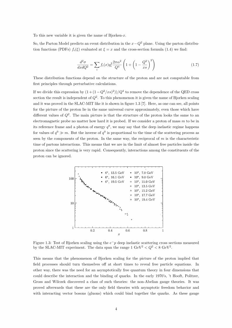
If we divide this expression by (1 + (1−Q2/xs)2))/Q4 to remove the dependence of the QED crosssection the result is independent of Q2. To this phenomenon it is given the name of Bjorken scalingand it was proved in the SLAC-MIT like it is shown in figure 1.3 [7]. Here, as one can see, all pointsfor the picture of the proton lie in the same universal curve approximately, even those which havedifferent values of Q2. The main picture is that the structure of the proton looks the same to anelectromagnetic probe no matter how hard it is probed. If we consider a proton of mass m to be inits reference frame and a photon of energy q0, we may say that the deep inelastic regime happensfor values of q0 m. But the inverse of q0 is proportional to the time of the scattering process asseen by the components of the proton. In the same way, the reciprocal of m is the characteristictime of partons interactions. This means that we are in the limit of almost free particles inside theproton since the scattering is very rapid. Consequently, interactions among the constituents of theproton can be ignored.
Figure 1.3: Test of Bjorken scaling using the e−p deep inelastic scattering cross sections measuredby the SLAC-MIT experiment. The data span the range 1 GeV2 < Q2 < 8 GeV2.
This means that the phenomenon of Bjorken scaling for the picture of the proton implied thatfield processes should turn themselves off at short times to reveal free particle equations. Inother way, there was the need for an asymptotically free quantum theory in four dimensions thatcould describe the interaction and the binding of quarks. In the early 1970’s, ’t Hooft, Politzer,Gross and Wilczek discovered a class of such theories: the non-Abelian gauge theories. It wasproved afterwards that these are the only field theories with asymptotic freedom behavior andwith interacting vector bosons (gluons) which could bind together the quarks. As these gauge
4
theories confirm the Bjorken scaling they also predict some corrections to this when one goes to ahigher level of accuracy in measurements of DIS experiments. In this kind of theories, the couplingconstant is still non-zero at any finite value of q and the evolution of the coupling constant to zerois very slow: follows a logarithmic distribution in momentum. So, this corrections must be seenat some level and it was what happened in the 1970’s particle experiments. Bjorken scaling wasfound to be only an approximate relation, showing violations that correspond to a slow evolutionof the parton distributions fi(x) over a logarithmic scale in Q2. We will see this behavior withmore detail in chapter 2.
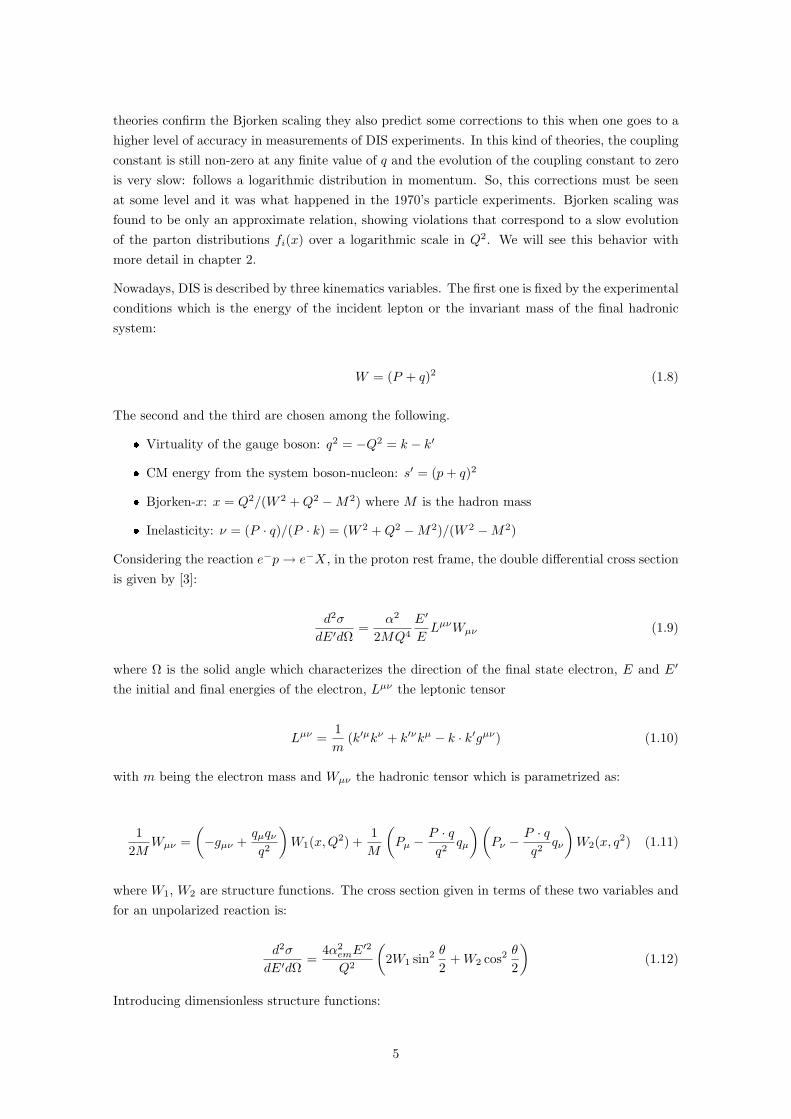
Nowadays, DIS is described by three kinematics variables. The first one is fixed by the experimentalconditions which is the energy of the incident lepton or the invariant mass of the final hadronicsystem:
W = (P + q)2 (1.8)
The second and the third are chosen among the following.
Virtuality of the gauge boson: q2 = −Q2 = k − k′
CM energy from the system boson-nucleon: s′ = (p+ q)2
Bjorken-x: x = Q2/(W 2 +Q2 −M2) where M is the hadron mass
Considering the reaction e−p→ e−X, in the proton rest frame, the double differential cross sectionis given by [3]:
d2σ
dE′dΩ=
α2
2MQ4
E′
ELµνWµν (1.9)
where Ω is the solid angle which characterizes the direction of the final state electron, E and E′
the initial and final energies of the electron, Lµν the leptonic tensor
Lµν =1m
(k′µkν + k′νkµ − k · k′gµν) (1.10)
with m being the electron mass and Wµν the hadronic tensor which is parametrized as:
12M
Wµν =(−gµν +
qµqνq2
)W1(x,Q2) +
1M
(Pµ −
P · qq2
qµ
)(Pν −
P · qq2
qν
)W2(x, q2) (1.11)
where W1, W2 are structure functions. The cross section given in terms of these two variables andfor an unpolarized reaction is:
d2σ
dE′dΩ=
4α2emE
′2
Q2
(2W1 sin2 θ
2+W2 cos2 θ
2
)(1.12)
Introducing dimensionless structure functions:
5
F1(x,Q2) = MW1(x,Q2)
F2(x,Q2) = νW2(x,Q2)(1.13)
the real inclusive double differential cross-section for the system is given by:
d2σ
dxdQ=
2πα2
xQ4
((1 + (1− y)2
)F2(x,Q2)− y2
(F2(x,Q2)− 2xF1(x,Q2)
))(1.14)
where y is the so called rapidity. It is defined in section 1.2.2, equation (1.23)
All information on the internal structure of the proton is encoded in these two structure functions,F1(x,Q2) and F2(x,Q2), as seen by the external probe. Scaling tell us that the structure functionsdepend only on one scaling variable, x, rather than on two as allowed by kinematics, taking us tothe Callan-Gross relation [14] where Fi(x,Q2)→ Fi(x) and F2(x) = 2xF1(x).
1.2 Quantum Chromodynamics (QCD)
QCD is a quantum field theory which describes the strong interaction, one of the four knownfundamental interactions in nature (gravitational, electromagnetic, weak and strong interactions)and is interpreted as the interaction between colour charged quarks where the colour is simplyanother kind of quantum number (red, blue and green) introduced to solve the problem of ∆++ [12].The forces between colour charged quarks are mediated by coloured field quanta, the gauge particlesbelonging to the local symmetry of the gauge theory called gluons. The only free parameters ofthe theory are the masses of the quarks and the strong coupling constant αs = g2/(4π), whichdetermines the strength of the interaction (coupling) between quarks and gluons.
In nature, all mesons and baryons are colorless which means that they must have equal amountsof colour and anti-colour or equal mixture of red, blue and green. Although an isolated quarkhad never been observed, the fact that hard interactions are well described by the quark modelmake us to believe that because the strong interaction is the most intense of the forces, no coloredstates can be observed. This property could be explained by the asymptotic freedom behavior, acharacteristic of a field theory with a non-Abelian gauge field.
1.2.1 Running Coupling and Perturbative QCD (pQCD)
QCD was born as a copy of QED where the mediator of the force is the photon which couple to theelectric charge, the electron, but is itself neutral. In QCD, the mediator is the gluon, which coupleto the colour charge, the quark, but unlike QED, gluons also carry colour charge leading to theso-called self-coupling of the gluon. In both theories there is the running of the coupling constantwhich make them dependent with the energy scale involved in the interaction. Physically, thisdependence is related to charge screening effects resulting from the vacuum polarization.
Lets suppose that we want to measure the charge of an electron in the vacuum. The electroncan radiate photons continuously which, by its turn, can split into positron-electron pairs. Thepositrons are attracted preferentially closer to the original electron meanwhile the other electrons
6
+
+
+
+
+
+
−
−
−
−
−
−
+
+
++
−
−
−−
e1
(a)
+
+
+
+
+
+
−
−−
−
−
−
e2
(b)
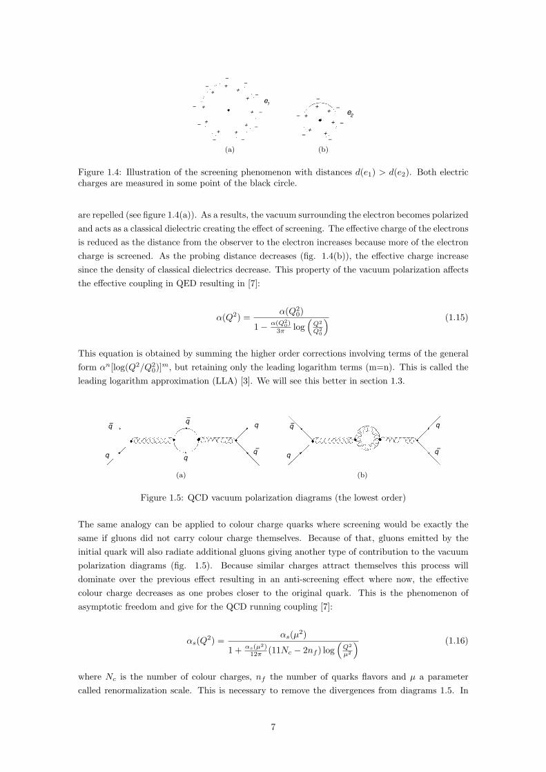
Figure 1.4: Illustration of the screening phenomenon with distances d(e1) > d(e2). Both electriccharges are measured in some point of the black circle.
are repelled (see figure 1.4(a)). As a results, the vacuum surrounding the electron becomes polarizedand acts as a classical dielectric creating the effect of screening. The effective charge of the electronsis reduced as the distance from the observer to the electron increases because more of the electroncharge is screened. As the probing distance decreases (fig. 1.4(b)), the effective charge increasesince the density of classical dielectrics decrease. This property of the vacuum polarization affectsthe effective coupling in QED resulting in [7]:
α(Q2) =α(Q2
0)
1− α(Q20)
3π log(Q2
Q20
) (1.15)
This equation is obtained by summing the higher order corrections involving terms of the generalform αn[log(Q2/Q2
0)]m, but retaining only the leading logarithm terms (m=n). This is called theleading logarithm approximation (LLA) [3]. We will see this better in section 1.3.
q−
q
q
q
q
q
−
−
(a)
q−
q
q
q−
(b)
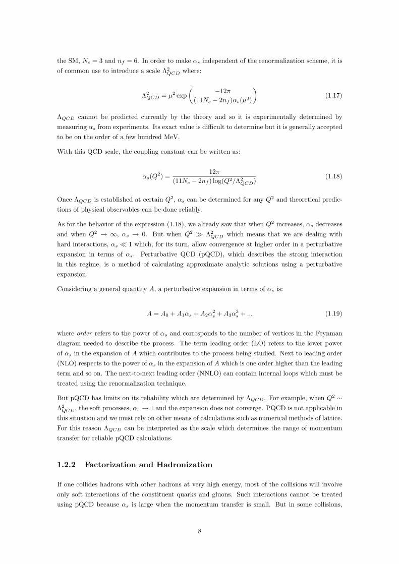
Figure 1.5: QCD vacuum polarization diagrams (the lowest order)
The same analogy can be applied to colour charge quarks where screening would be exactly thesame if gluons did not carry colour charge themselves. Because of that, gluons emitted by theinitial quark will also radiate additional gluons giving another type of contribution to the vacuumpolarization diagrams (fig. 1.5). Because similar charges attract themselves this process willdominate over the previous effect resulting in an anti-screening effect where now, the effectivecolour charge decreases as one probes closer to the original quark. This is the phenomenon ofasymptotic freedom and give for the QCD running coupling [7]:
αs(Q2) =αs(µ2)
1 + αs(µ2)12π (11Nc − 2nf ) log
(Q2
µ2
) (1.16)
where Nc is the number of colour charges, nf the number of quarks flavors and µ a parametercalled renormalization scale. This is necessary to remove the divergences from diagrams 1.5. In
7
the SM, Nc = 3 and nf = 6. In order to make αs independent of the renormalization scheme, it isof common use to introduce a scale Λ2
QCD where:
Λ2QCD = µ2 exp
(−12π
(11Nc − 2nf )αs(µ2)
)(1.17)
ΛQCD cannot be predicted currently by the theory and so it is experimentally determined bymeasuring αs from experiments. Its exact value is difficult to determine but it is generally acceptedto be on the order of a few hundred MeV.
With this QCD scale, the coupling constant can be written as:
αs(Q2) =12π
(11Nc − 2nf ) log(Q2/Λ2QCD)
(1.18)
Once ΛQCD is established at certain Q2, αs can be determined for any Q2 and theoretical predic-tions of physical observables can be done reliably.
As for the behavior of the expression (1.18), we already saw that when Q2 increases, αs decreasesand when Q2 → ∞, αs → 0. But when Q2 Λ2
QCD which means that we are dealing withhard interactions, αs 1 which, for its turn, allow convergence at higher order in a perturbativeexpansion in terms of αs. Perturbative QCD (pQCD), which describes the strong interactionin this regime, is a method of calculating approximate analytic solutions using a perturbativeexpansion.
Considering a general quantity A, a perturbative expansion in terms of αs is:
A = A0 +A1αs +A2α2s +A3α
3s + ... (1.19)
where order refers to the power of αs and corresponds to the number of vertices in the Feynmandiagram needed to describe the process. The term leading order (LO) refers to the lower powerof αs in the expansion of A which contributes to the process being studied. Next to leading order(NLO) respects to the power of αs in the expansion of A which is one order higher than the leadingterm and so on. The next-to-next leading order (NNLO) can contain internal loops which must betreated using the renormalization technique.
But pQCD has limits on its reliability which are determined by ΛQCD. For example, when Q2 ∼Λ2QCD, the soft processes, αs → 1 and the expansion does not converge. PQCD is not applicable in
this situation and we must rely on other means of calculations such as numerical methods of lattice.For this reason ΛQCD can be interpreted as the scale which determines the range of momentumtransfer for reliable pQCD calculations.
1.2.2 Factorization and Hadronization
If one collides hadrons with other hadrons at very high energy, most of the collisions will involveonly soft interactions of the constituent quarks and gluons. Such interactions cannot be treatedusing pQCD because αs is large when the momentum transfer is small. But in some collisions,
8
however, the most likely interaction is that a parton in one hadron interacts with a parton in theother hadron which destroys the hadron structure. This is represented in figure 1.6.
P1
P2
fi(x
1)
fj(x
2)
p1= x
1P
1
p2= x
2P
2
i j s)
^
Figure 1.6: The parton model description of a hard scattering process
In this situation, both partons participating in the interaction exchange a large momentum per-pendicular to the collision axis, p⊥, and then, as in DIS, the elementary interaction takes placevery rapidly compared to the internal time scale of the hadron wave functions. So, the lowest-orderQCD prediction should accurately describes the process and again, we must find a parton-modelformula that is built from a leading-order subprocess cross section, integrated with PDFs. Thedifferential cross section for a hard scattering process initiated by two hadrons with 4-momenta P1
and P2 takes the form:
dσh
d2p⊥dy(P1, P2) =
∫ 1
0
dx1
∫ 1
0
dx2
∑i,j
fi(x1, µ2)fj(x2, µ
2)dσij→k
dt
(p1, p2, α(µ2), Q2/µ2
)Dk→h(z, µ2)
(1.20)
where the sum runs over all species of partons. The momenta of the partons which participate inthe hard scattering are p1 = x1P1 and p2 = x2P2, while Q is the characteristic scale of the hardprocess and fi(j)(x1(2)) are the usual QCD PDFs of quarks and gluons inside the hadrons, definedat a factorization scale µ. This is an arbitrary parameter and can be thought as the scale whichseparates the long distance regime from the short one. Thus, a parton emitted with small transversemomentum, less than the scale µ, is considered part of the hadron structure and is absorbed intothe parton distribution. If has a large transverse momentum, then is part of the short distancecross section. This scale should be chosen to be of the order of the hard scale Q.
The short distance cross section for the scattering of partons of types i and j is denoted by σij→k.Since the coupling constant is small at high energies, the short distance cross section can becalculated as a perturbation series in the running coupling αs. In the leading approximation, thisis identical do the normal parton scattering cross section, but in higher orders it is acquired byremoving long distance pieces and putting them into the PDFs. This is necessary because the crosssection calculated by perturbation theory contains contributions form interactions which occur longbefore the hard scattering. These pieces can be factorized and absorbed into the description of theincoming hadrons.
Quarks and gluons not involved in the hard scattering are termed the spectators and continueapproximately in the beam direction carrying off very little transverse momenta. As for the two
9
objects participating in the hard scatter, they are ejected from the proton in a manner that cannotbe balanced by subsequent soft processes. Because they cannot break free, soft processes will creategluons and quark-antiquark pairs that eventually neutralize the colour causing bound colorlesshadrons to emerge. To this process is called hadronization or fragmentation and is not very wellunderstood yet. There are at least three classes of models [15] (Independent fragmentation, Stringmodel and Cluster model) which are incorporated in Monte Carlo programs like PYTHIA [16]and HERWIG [17] that try to simulate the process until a final observable state: hadrons. Thisinformation is encoded in the fragmentation function Dk→h with k being the parton with fractionof momentum z that will hadronize into a hadron h.
With this, our cross section can be factorized in three components (one hard + two soft terms):
Cross section of partonic subprocesses like quarks, boson and leptons: This is a perturbativequantity calculated by perturbative methods (pQCD);
PDFs of hadrons: Are non-perturbative quantities which have information of objects beforecollision.
Fragmentation Functions (FFs): Another non-perturbative quantities and are related to thehadronization mechanism of partons.
The last two components must be known is order to predict some results of observable quantities.Fortunately these quantities are universal and do not depend of the process. For this reason, theycan be extracted from experiments where we already know the cross section for the elementarysubprocess.
Both PDFs and FFs are dynamical evolutional quantities because, as we seen, Bjorken scaling isbroken. In order to treat this violation we will use DGLAP formalism which we will see in chapter2.
1.2.3 Jet Production
Those hadrons that emerge from the hard scattering process have large transverse momentumand travel approximately in the same direction as the scattered quark or gluon. This collimatedspray of particles around the direction of flight of the original partons is known as a jet [7,15,18].By measuring their properties we hope to determine the properties of its parent partons, such asdirection and quantum numbers (spin, flavour) making them an important tool for testing QCD.For example, in the CM frame, a reaction like e+e− → qq will generally produce two jets back-to-back. But if one of the two quarks radiates a hard gluon, the event will appear as a three-jetevent. The observation of this kind of event was one of the greatest triumphs of QCD because theangular distribution was found to be consistent with the radiation of a spin 1 particle as expectedfor gluon bremsstrahlung [19].
Unfortunately it is very difficult to distinguish hadronic jets initiated by gluons from those initiatedby quarks. For this reason, it is very important to find variables capable of characterize a jet. TheCM of the parton-parton collision is usually in motion or boosted with respect to the CM ofthe colliding hadrons. Therefore, the right choice of variables used to describe jets are the oneswhich transform simply under longitudinal boosts: rapidity (y), transverse momentum (p⊥) andazimuthal angle (φ). With these variables, the 4-momentum of a particle with mass m is:
10
pµ = (mT cosh(y), p⊥ sinφ, p⊥ cosφ, mT ) (1.21)
where the transverse mass is defined as
mT =√p2⊥ +m2 (1.22)
The rapidity is given by:
y =12
ln(p0 + p3
p0 − p3
)=
12
ln(E + pzE − pz
)(1.23)
and is additive under Lorentz transformation corresponding to boosts along the z direction. Sincethe mass of the particle might be unknown, a more easily measured variable is pseudorapidity (η),an approximation only valid when the mass of the particle is almost zero when compared to itsmomentum:
y '= − ln[tan
(θ
2
)]≡ η (1.24)
Also, a more convenient experimental observable is the transverse energy
ET = E sin θ (1.25)
rather than pT since it is the quantity measured in a hadron calorimeter.
The jet shape will be affected by these variables: for E⊥ changes, the transverse momentum ofa particle, as measured from the jet axis, changes slowly while the parallel momentum changesapproximately with energy. Forward (or high η) jets are expected to be narrower than central(η ∼ 0) ones for the same E⊥. Also, quark jets are expected to be narrower than gluon jetsbecause gluons, carrying more colour than quarks, emit gluons more readily tending to widen thejet.
1.2.4 QCD Bremsstrahlung
A hard process can be said to occur when a quark is knocked out from the vacuum or from ahadron, as in DIS processes, as a bare particle, or more accurately, as a half-dressed one since itpossesses its own privative field. This means that a charge, when being accelerated, appears to havea truncated proper field, or mathematically speaking, has its Fourier components with k⊥ <
√Q2.
Because of this, subsequently two closely correlated processes start: the first is bremsstrahlungradiation and the second is the regeneration of the privative gluonic field of the parent quark.This regeneration phenomenon has been well understood in QED and the analogy with QCD isstraightforward.
The regeneration time Tregen of the proper field, which means, its Fourier components with mo-mentum k, is given by [3]:
11
Tregen(k) ∼k‖
k2⊥
(1.26)
where the longitudinal (k‖) and transverse (k⊥) components of the photon momentum are definedwith respect to the outgoing electron. So, a photon with a relatively small transverse momentak⊥ < k‖ ∼ p ∼ E where E and p stands for the momentum and energy of the electron, may see itsregeneration time become macroscopically large. The finiteness of this regeneration time leads tocurious effects for relativistic electrons such as Landau-Pomeranchuck-Migdal (LPM) effect whichwill be discussed later in section 3.3. As an illustrative example let us consider a scatter of a fastelectron at a large angle. We know that two cones of bremsstrahlung photon radiation are formed(fig. 1.7(a)): the quanta from the first cone, centered around the direction of the initial electronmomentum, is the Cerenkov radiation and the second cone is the back of the regeneration of a newproper field. For a double scattering, it might seem natural to expect an appearance of four photoncones (fig. 1.7(b)). However, this is only true if the regeneration length, cTregen, is less than thedistance between two successive scattering points ∆x. Otherwise, only two of them will actuallyemerge because the field has no time to regenerate itself and consequently, no electromagneticsurrounding can shaken the medium creating a second bremsstrahlung cone (fig. 1.7(c)).
(a) (b) (c)
Figure 1.7: Formation of Cerenkov radiation and field regeneration. Single scattering (a) anddouble scattering with cTregen < ∆x (b) and with cTregen > ∆x (c)
As for QCD bremsstrahlung, the differential spectrum of gluon radiation off a quark differs fromthe ordinary spectrum of a photon emitted by an electron only by the colour factor CF = (N2
c −1)/2Nc = 4/3 and, of course, by the substitution α→ αs [3]:
dωq→qg =αs(k2
⊥)4π
2CF
[1 +
(1− k
E
)2]dk
k
dk2⊥
k2⊥
(1.27)
where kµ is the 4-momentum of the gluon.
There is two important properties of the QCD bremsstrahlung phenomenon which must be high-lighted: a broad logarithmic distribution over transverse momentum which means there is a highprobability of obtain a quasicollinear quark-gluon configurations; and a broad logarithmic energydistribution, which means a high probability for low energies configurations. These basic proper-ties are in connection with divergences, called collinear divergency (or mass singularity) and softdivergency (or Infrared (IR) singularity), revealing an explosion to infinity of the probability ofemission when the angle or the energy goes to zero.
Thus, in order to acquire a large total emission probability, in spite of αs being small, we can
12
pick at least one logarithmic integration out of the perturbative phase space. The list of possibleorderings are:
R−1 k⊥ k ∼√Q2 which is the quasicollinear hard parton splitting leading to the
known scaling violation effects is DIS;
R−1 k⊥ ∼ k √Q2, a large angle soft gluon emission responsible for QCD coherence
phenomena;
R−1 k⊥ k √Q2, a soft and collinear gluon bremsstrahlung characterized by a double
logarithm.
1.3 Basic Idea of the Leading Logarithm Approximation
(LLA)
Gribov and Lipatov [20] showed that, in a field theory with dimensionless coupling constant g, DISstructure functions are represented as a sum of Rutherford cross-sections of lepton scattering ona point-like charged particle, weighted by parton densities Df
i (x), where x is the fraction of thelongitudinal momentum p of the fast projectile i carried by the parton f :
DIS structure functions =∑
σRuth(lepton scatter) ·Dfi (x) (1.28)
As we saw in section 1.1. logarithmic deviations from the true scaling behavior had been pre-dicted for the PDFs, revealing the internal structure of parton densities which are correctly givenby Df
i (x, logQ2). This Q dependence comes from summing the leading logarithmic corrections.Physically represents the fact that a DIS involving a photon of virtuality Q2 corresponds to thescattering of that virtual photon on a quark of transverse size 1/Q. The point is that Q2 setsan upper bound for transverse momenta of partons logarithmic distributed over the broad range.From equation (1.27)
dω ∝ g2
∫ Q2dk2⊥
k2⊥
(1.29)
This makes the total probability of extra parton production large:
g2 1, logQ2 high enough⇒ ω ∝ g2 logQ2 ∼ 1 (1.30)
This observation formed the base of the so called LLA. In this framework, one keeps trace ofcontributions to structure functions of the order
W (x,Q2) ∝ Dfi (x, logQ2) =
∞∑n=0
fn(x)(αsπ
logQ2)n
(1.31)
while neglecting systematically corrections of the relative order αs, not accompanied by a largelogarithm.
13
In a field theory, with asymptotic freedom, such an approximation proves to be asymptoticallyexact:
W true(x,Q2) = WLLA(x,Q2)[1 + O
(αs(Q2)π
)]Q2→∞−−−−−→WLLA(x,Q2) (1.32)
So, the LLA parton wave function of a projectile is built by interacting elementary parton splittingprocesses 1→ 2 with successive increasing momenta:
µ2 k2⊥1 k2
⊥2 · · · k2⊥n−1 k2
⊥n Q2 (1.33)
This is called the strong transverse momentum ordering and is necessary to gain the maximallogarithmic contribution to W (x,Q2) in the nth perturbative order. Physically, it means thatpartons are not point-like particles because an attempt to localize the parton of the ith generationwhich has a typical transverse size 1/k⊥i, reveals its substructure at smaller distances 1/k⊥i+1 1/k⊥i.
14
Chapter 2
Evolution Equations
As seen in the previous chapter, the structure of a hadron evolve with energy Y = log(1/x) andwith virtuality Q2. As a result, its configuration changes and although the hadron itself is nolonger a perturbative object for many values of (Q2, x), its evolution is still perturbative, exceptfor low values of Q2. It is based on this observation that many people have constructed evolutionequations capable of describing the evolution of this kind of objects in the two variables of thephase space. Unfortunately, it is still impossible to describe all directions and so, in the nextparagraphs it follows a general description of the phase space defined by (Q2, x) and the principalevolution equations up to now.
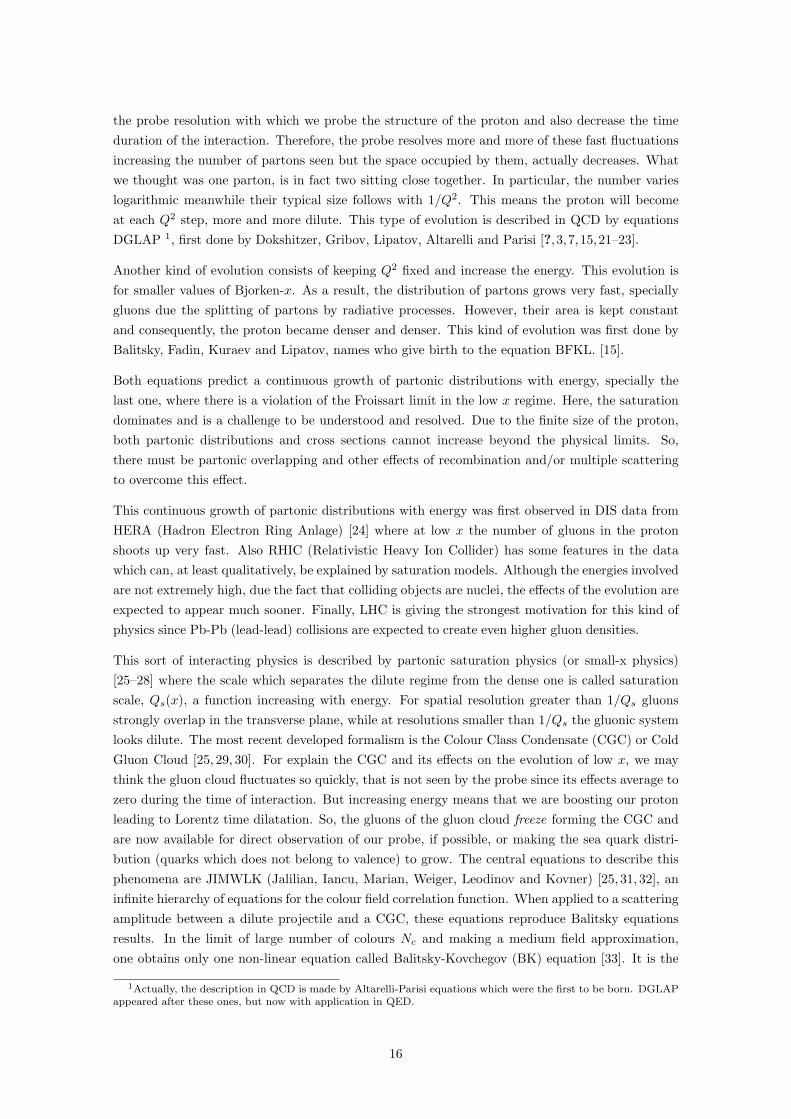
Figure 2.1: Schematic representation of the proton in the phase space defined by (Q2, x)
In figure 2.1 it is showed the diagrammatic representation of the proton in different regions ofits phase space. Initially, when Q2 and Y are small, the proton is represented by three valencequarks, which are surrounded by a gluon cloud fluctuating very quickly. We may think of thisfluctuations as vacuum oscillations. If we keep the energy fixed and increase Q2, we increase
15
the probe resolution with which we probe the structure of the proton and also decrease the timeduration of the interaction. Therefore, the probe resolves more and more of these fast fluctuationsincreasing the number of partons seen but the space occupied by them, actually decreases. Whatwe thought was one parton, is in fact two sitting close together. In particular, the number varieslogarithmic meanwhile their typical size follows with 1/Q2. This means the proton will becomeat each Q2 step, more and more dilute. This type of evolution is described in QCD by equationsDGLAP 1, first done by Dokshitzer, Gribov, Lipatov, Altarelli and Parisi [?,3,7,15,21–23].
Another kind of evolution consists of keeping Q2 fixed and increase the energy. This evolution isfor smaller values of Bjorken-x. As a result, the distribution of partons grows very fast, speciallygluons due the splitting of partons by radiative processes. However, their area is kept constantand consequently, the proton became denser and denser. This kind of evolution was first done byBalitsky, Fadin, Kuraev and Lipatov, names who give birth to the equation BFKL. [15].
Both equations predict a continuous growth of partonic distributions with energy, specially thelast one, where there is a violation of the Froissart limit in the low x regime. Here, the saturationdominates and is a challenge to be understood and resolved. Due to the finite size of the proton,both partonic distributions and cross sections cannot increase beyond the physical limits. So,there must be partonic overlapping and other effects of recombination and/or multiple scatteringto overcome this effect.
This continuous growth of partonic distributions with energy was first observed in DIS data fromHERA (Hadron Electron Ring Anlage) [24] where at low x the number of gluons in the protonshoots up very fast. Also RHIC (Relativistic Heavy Ion Collider) has some features in the datawhich can, at least qualitatively, be explained by saturation models. Although the energies involvedare not extremely high, due the fact that colliding objects are nuclei, the effects of the evolution areexpected to appear much sooner. Finally, LHC is giving the strongest motivation for this kind ofphysics since Pb-Pb (lead-lead) collisions are expected to create even higher gluon densities.
This sort of interacting physics is described by partonic saturation physics (or small-x physics)[25–28] where the scale which separates the dilute regime from the dense one is called saturationscale, Qs(x), a function increasing with energy. For spatial resolution greater than 1/Qs gluonsstrongly overlap in the transverse plane, while at resolutions smaller than 1/Qs the gluonic systemlooks dilute. The most recent developed formalism is the Colour Class Condensate (CGC) or ColdGluon Cloud [25, 29, 30]. For explain the CGC and its effects on the evolution of low x, we maythink the gluon cloud fluctuates so quickly, that is not seen by the probe since its effects average tozero during the time of interaction. But increasing energy means that we are boosting our protonleading to Lorentz time dilatation. So, the gluons of the gluon cloud freeze forming the CGC andare now available for direct observation of our probe, if possible, or making the sea quark distri-bution (quarks which does not belong to valence) to grow. The central equations to describe thisphenomena are JIMWLK (Jalilian, Iancu, Marian, Weiger, Leodinov and Kovner) [25, 31, 32], aninfinite hierarchy of equations for the colour field correlation function. When applied to a scatteringamplitude between a dilute projectile and a CGC, these equations reproduce Balitsky equationsresults. In the limit of large number of colours Nc and making a medium field approximation,one obtains only one non-linear equation called Balitsky-Kovchegov (BK) equation [33]. It is the
1Actually, the description in QCD is made by Altarelli-Parisi equations which were the first to be born. DGLAPappeared after these ones, but now with application in QED.
16
most simple equation which describes QCD in the high energy regime and it is formed by thelinear equation BFKL plus an additional non-linear term responsible by the decrease of gluonicdensity.
2.1 Altarelli-Parisi Equations
To make a derivation of this set of equations, it is easier to begin by studying the case of collineargluon emission at high energies since the phenomena associated with mass singularities is presentin here. This will result in an enhancement of higher-order terms which cannot be neglected inperturbative calculations.
Some Feynman diagrams with mass singularities associated with collinear gluon emission are drawnin figure 2.2. These are examples of the traditional (multiple) Compton scattering which givecontribution to the LLA, the base mathematical method to obtain DGLAP. Generally, all diagramswith mass singularities associated with one collinear emission are one of the forms shown in figure2.3, where the circle represents a scattering process with large momentum transfer.
f
f
(a)
f
f
(b)
Figure 2.2: Some examples with mass singularities: leading order (a) and higher order (b) diagrams.
p
q
k
X
Y
(a) DIS of a quark
p
q
k
X
Y
(b) DIS of a gluon
Figure 2.3: General form of diagrams with mass singularities.
Mass singularities appear when the denominator of the intermediate propagator goes to zero,that is, when the intermediate state is almost on-shell. This means that we can interpret thefirst diagram as a transition to a real gluon and an almost-real quark (fermion) followed by theinteraction of the quark with all remaining particles. For the second diagram we can have a similarinterpretation but with an almost-real gluon in the intermediate state and a real quark. The onlyquestion is how to define the polarization of these intermediate state particles.
For a quark, the numerator of the propagator is
/k =∑s
us(k)us(k) (2.1)
17
with us(k)(vs(k)) spinors for a quark (anti-quark) of spin s and momentum k. In the masslesslimit, they are the same. So when k2 → 0, the gluon emission vertex and the remaining part ofthe amplitude are contracted with on-shell polarization spinors.
The numerator of the gluon propagator is given by the relation:
gµν = ε−µ ε+∗ν + ε+µ ε
−∗ν −
∑i
εTiµεT∗iν (2.2)
Both forward (ε+) and backward (ε−) polarizations are proportional to the gluon momentumqµ:
ε+µ (k) =(
k0
√2|k|
,k√2k
), ε+µ (k) =
(k0
√2|k|
,− k√2k
)(2.3)
So, using the Ward Identity [7], which tell us that if M(k) = εµ(k)Mµ(k) is the amplitude for someQCD process involving an external gluon with momentum k and polarization εµ(k), then:
M(k) = εµ(k)Mµ(k)⇒ kµMµ(k) = 0 (2.4)
we will get a null result when contracting these polarizations with QCD scattering amplitude onthe right. This means that when the gluon momentum q goes on-shell, we may replace
−igµν
q2 + iε→ i
q2 + iε
∑i
εµTiε∗νTi (2.5)
p
q
k
1
3^
^
A
A’
Figure 2.4: Kinematics for the collinear emission vertex
Now we are able to decouple the gluon or quark emission vertex from the rest of the diagramand evaluated it explicitly with physical polarization states of massless particles. The kinematicchosen is shown in figure 2.4 where the final particles should be almost collinear. If z ∈ [0, 1] isthe fraction of the initial quark energy carried by the gluon and p⊥ the transverse momenta of thefinal particles which is assumed to be small since we are dealing with almost collinear emissions,the three 4-momenta are:
p = (p, 0, 0, p) (2.6a)
q ≈ (zp, p⊥, 0, zp) (2.6b)
k ≈ ((1− z)p, −p⊥, 0, (1− z)p) (2.6c)
which means that:
18
p2 = 0 and q2 = k2 = 0 + O(p2⊥) (2.7)
But is more formally correct to make the real particle more real and the virtual particle slightlyoff-shell. So, for a real gluon we can write:
p = (p, 0, 0, p) (2.8a)
q ≈(zp, p⊥, 0, zp− p2
⊥2zp
)(2.8b)
k ≈(
(1− z)p, −p⊥, 0, (1− z)p+p2⊥
2zp
)(2.8c)
which implies that:
p2 = 0 (2.9a)
q2 = 0 + O(p4⊥) (2.9b)
k2 ∝ p2⊥ + O(p4
⊥) (2.9c)
and for a real quark:
p = (p, 0, 0, p) (2.10a)
q ≈(zp, p⊥, 0, zp− p2
⊥2(1− z)p
)(2.10b)
k ≈(
(1− z)p, −p⊥, 0, (1− z)p+p2⊥
2(1− z)p
)(2.10c)
making:
p2 = 0 (2.11a)
q2 ∝ p2⊥ + O(p4
⊥) (2.11b)
k2 = 0 + O(p4⊥) (2.11c)
But before we proceed to the evaluation of the matrix element for this splitting process, we canwork with the light-cone basis (see Appendix A) instead of Dirac basis since the causality becomesautomatically resolved. Also, this gauge is of common use in the present area of research discussedin this thesis and to keep a certain consistency with the rest, we will make a transformation ofMinkowski coordinates to the light-cone ones.
19
Thus, the kinematics for a real gluon is now
p =(√
2p, 0, 0)
(2.12a)
q ≈
(√
2zp−√
2p2⊥
4zp,
√2p2⊥
4zp, p⊥, 0
)(2.12b)
k ≈
(√
2(1− z)p+√
2p2⊥
4zp, −√
2p2⊥
4zp, −p⊥, 0
)(2.12c)
and for a real quark:
p =(√
2p, 0, 0)
(2.13a)
q ≈
(√
2zp+√
2p2⊥
4(1− z)p, −
√2p2⊥
4(1− z)p, p⊥, 0
)(2.13b)
k ≈
(√
2(1− z)p−√
2p2⊥
4(1− z)p,
√2p2⊥
4zp, −p⊥, 0
)(2.13c)
In order to get ε · q = 0 up to terms of order p2⊥ and |ε|2 = −1, we may choose for the gluon
polarization:
ε(i) =(
0,q⊥ · ε(i)⊥
q+, ε(i)⊥
)(2.14)
where ε(R)⊥ = 1√2(−1, −i) and ε(L)⊥ = 1√
2(1, −i) are the right and left transverse polariza-
tions.
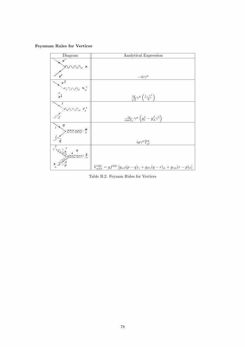
The matrix element for the QCD vertex is simply (see Appendix B for Feynman rules in QCD):
M = igT aA′Au(k)γµu(p)ε∗µ(q) (2.15)
where T aA′A are the generators of the symmetry group. The colour indices A′, A corresponds tothe quark in the final and initial state respectively and the index a to the gluon.
We have to specify all four possible helicities but parity invariance implies that:
M(fL → fLgR) = M(fR → fRgE) (2.16)
M(fL → fLgL) = M(fR → fRgR) (2.17)
where f refers to the quark and g to the gluon.
This means we only need to compute two of them. With the helicity of quarks
20
χ(p) = χ(k) =1√2
010−1
, χ(k) =1√2
p⊥
2p(1−z)
1− p⊥
2p(1−z)
−1
(2.18)
and after some algebra we obtain the amplitude results:
M(fL → fLgR) = −igT aA′A
√2(1− z)z
p⊥ (2.19)
M(fL → fLgL) = −igT aA′A
√2(1− z)z(1− z)
p⊥ (2.20)
By averaging over initial colored states, sum over final colored states in order to obtain the colourfactor and doing the same for the spin, we get the squared matrix average (see Appendix C for thecolour algebra):
|M|2 =12
1dA
∑pol,a
|M|2 =12
1dA
(2|M(e−L → w−LγR)|2 + 2|M(e−L → w−LγL)|2
)=
=1
d(N)Tr[T aT a]
2e2(1− z)z2
p⊥
(1 +
1(1− z)2
)= CF
2e2p2⊥
z(1− z)
((1− z)2 + 1
z
)(2.21)
where dA = d(N) is the dimension of the representation and CF = (N2c − 1)/(2Nc) is the second
Casimir, both for the fundamental representation. Nc is the number of colours.
2.1.1 Gluon Distribution
The total cross-section for a process 1 + 2→ 3 + 4 is given by:
σ =∫
1
4√
(p1 · p2)2 −m21m
22
|Mfi|2(2π)4δ4(p1 + p2 − p3 − p4)d3p3
2p03(2π)3
d3p4
2p04(2π)3
(2.22)
The first term is the kinematic from the initial state, the |Mfi|2 is the amplitude of the wholeprocess, the δ-function together with the factor (2π)4 expresses the conservation of the energy-momentum and the rest is the phase space of the final sate. For our process of a virtual quark weshould have p+X → k + Y . We begin by evaluating all terms separately:
Hence, the total cross-section can be written as (conservation of energy-momentum is implicit):
σ(fX → fY ) =∫
1(1 + vX)2p2EX
|M|2(
1q2
)2
|MgX |2d3k
(2π)3
12k0
dΠY =
=∫dzdp2
⊥8π
g2
p2⊥CF
(1 + (1− z)2
z
)∫1
2zpEX(1 + vX)dΠY |MgX |2 =
=∫ 1
0
dz
∫ s
m2
dp2⊥
p2⊥
αs2πCF
(1 + (1− z)2
z
)σ(gX → Y ) =
=∫ 1
0
dzαs2π
log( s
m2
)CF
(1 + (1− z)2
z
)σ(gX → Y ) (2.35)
Our final result tell us that the probability to occur the reaction fX → fY is equal to theprobability to occur the reaction gX → Y weighted by a distribution function that give us theprobability of finding a gluon of longitudinal fraction z in the incident quark. This is anotherexample of factorization like in equation (1.20) except that here we have a collision quark-hadronrather than hadron-hadron. The FF and elementary cross-section are contained in σ(gX → Y )remaining only one PDF:
22
fg(z) =αs2π
log( s
m2
)CF
(1 + (1− z)2
z
)(2.36)
2.1.2 Quark Distribution
The previous case was for the diagram in which the gluon is virtual and the quark a real particle.Now, we will write the cross section for the first diagram in which the gluon is real and the quarkis virtual. The cross section will be analogue to equation (2.35):
σ(fX → gY ) =∫
1(1 + vX)2p2EX
|M|2(
1k2
)2d3q
(2π)3
12q0
dΠY∫dz dp2
⊥8π
g2
p2⊥CF
(1 + (1− z)2
z
)∫1
2(1− z)p2EX(1 + vX)dΠY |MfX |2 =∫ 1
0
dz
∫ s
m2
dp2⊥
p2⊥
αs2πCF
(1 + (1− z)2
z
)σ(fX → Y ) (2.37)
where the intermediate quark carries a longitudinal fraction (1 − z) and k2 = p2⊥/z. For the
distribution function of finding a quark parton in the quark, we could substitute x→ (1− z) andobtain:
f(1)f (x) =
αs2π
log( s
m2
)CF
(1 + x2
1− x
)(2.38)
However this expression is not complete for it does not have into account the process withoutradiation, when the quark remains with its full energy or simply emit soft gluons which does notaffect the rate of QCD reaction: x → 1 ⇒ f
(1)f (x) → ∞. We could simply add to the previous
expression this case:
f(2)f (x) = δ(1− x) +
α
2πlog( s
m2
)CF
(1 + x2
1− x
)(2.39)
but still it is not correct because it is not a normalized expression. Thus, we have to subtract whatwe add and since IR divergences are canceled order by order in αs, we may have:
ff (x) = δ(1− x) +α
2πlog( s
m2
)CF
(1 + x2
1− x−Aδ(1− x)
)(2.40)
The parameter A is determined by the condition:
∫ 1
0
dxff (x) = 1 (2.41)
In order to skirt the singularity one defines a new distribution:
1(1− x)+
=1
(1− x)∀ x ∈ [0, 1[ (2.42)
23
∫ 1
0
dxf(x)
(1− x)+=∫ 1
0
dxf(x)− f(1)
1− x(2.43)
With this, we can find A = −3/2 and get as a final result, the quark distribution to order αs:
ff (x) = δ(1− x) +α
2πlog( s
m2
)CF
(1 + x2
1− x+
32δ(1− x)
)(2.44)
2.1.3 Evolution Equations
Both quark and gluon distributions can be part of a continuous evolution process of the initialprobe. Considering the case of multiple collinear emission (fig. 2.5) we can use the LLA toevaluate its contribution and only when p1⊥ p2⊥ p3⊥ ... we get similar quantities to αsfor higher orders.
X
Y1
2
3
.
.
.
Figure 2.5: Higher order diagram with collinear gluon emission
The contribution is of order
(αs2π
)n ∫ s
m2
dp21⊥
p21⊥
∫ p21⊥
m2
dp22⊥
p22⊥· · ·∫ dp2n−1⊥
m2
dp2n⊥
dp2n⊥
=1n!
(αs2π
)nlogn
( s
m2
)(2.45)
We can interpret this result as seeing the quark at resolutions that increase in each step and as aconsequence, resolve it into a more virtual quark and more gluons. To express this evolution anddependence with transverse momentum of the constituent quark, it is usual to introduce fg(x,Q)and ff (x,Q). They define the probability of finding a gluon or a quark of longitudinal fractionx in the physical quark taking into account collinear gluon emission with transverse momentump⊥ < Q. The differential equation for a quark split off a gluon carrying a fraction z of its energyis:
(αs2π
) dp2⊥
p2⊥CF
(1 + (1− z)2
z
)(2.46)
But if Q is slightly increased to Q+ ∆Q which means we are analyzing the particle with a betterresolution, we make visible more constituents of the physical wave function. In this situation, wemust take into account that a quark constituent in ff (x,Q) will radiate a gluon with Q < p⊥ <
Q+ ∆Q. The new gluon distribution is the initial one plus a little contribution:
24
fg(x,Q+ ∆Q) = fg(x,Q) +∫ 1
0
dx′∫ 1
0
dz(αs
2π
) ∆Q2
Q2CF
(1 + (1− z)2
z
)ff (x′, p⊥)δ(x− zx′)
(2.47)
The ff (x′, p⊥) tell us that the new gluon comes from a quark constituent which have to carry alarger longitudinal component in order to emitt more energetic gluons (δ(x′ − zx)).
Noting that:
δ(x′ − zx) = δ[z(xz− x′
)]=
1zδ(xz− x′
)(2.48)
if we want 0 ≤ x′ ≤ 1, we have to have x < z < 1. Making ∆Q2 ≡ dQ2 = 2QdQ, we maywrite:
fg(x,Q+ ∆Q) = fg(x,Q) +∫ 1
0
dx′∫ 1
0
dz∆QQ
CF1 + (1− z)2
zff (x′, p⊥)
1zδ(xz− x′
)=⇔
⇔ fg(x,Q+ ∆Q) = fg(x,Q) +∆QQ
∫ 1
x
dz
z
(αsπCF
1 + (1− z)2
z
)ff
(xz, p⊥
)⇔
⇔ d
d logQfg(x,Q) =
∫ 1
x
dz
z
(αsπCF
1 + (1− z)2
z
)ffe
(xz,Q)
(2.49)
So, the gluon distribution in the quark is governed by this integral-differential formula. The quarkdistribution inside the initial quark will evolve in the same way, reflecting the appearance of quarksat lower values of x when increasing Q. This is caused by gluon radiation and the disappearanceof these quarks at higher x:
d
d logQff (x,Q) =
∫ 1
x
dz
z
[αsπCF
(1 + z2
(1− z)++
32δ(1− z)
)]ff
(xz,Q)
(2.50)
With this, cross sections (2.35) and (2.37) are now replaced by:
σ(fX → f + ng + Y ) =∫ 1
0
dxfg(x,Q)σ(gX → Y ) (2.51)
σ(fX → ng + Y ) =∫ 1
0
dxff (x,Q)σ(fX → Y ) (2.52)
where fg(x,Q) and ff (x,Q) are solutions of equations (2.49) and (2.50) and Q is chosen as acharacteristic momentum transfer of the gX or fX subprocess.
But in order to fully complete this evolution process, are necessary two more diagrams: the gluonsplitting into pairs, fig. 2.6(a) and the three-gluon vertex 2.6(b). Applying the same procedure asbefore for the first diagram of figure 2.6, one arrives at:
|M|2 =2e2
z(1− z)[(1− z)2 + z2
]p2⊥ (2.53)
25
p
q
k
A
A’
(a) Quark splitting process
pq
k
(b) Three-gluon vertex
1
3^
^
Figure 2.6: Kinematics of the remaining processes
where z is the momentum fraction carried by the antiquark. But when one creates a pair quark-antiquark, one must remove a gluon causing a negative contribution weighted by:
∫ 1
0
dz[(1− z)2 + z2
]=
23
(2.54)
For the vertex 2.6(b) we have to evaluate it. The element matrix is:
The colour factor for the squared averaged amplitude should be:
1da
∑b,c
fabcf∗abc = CA = 3 (2.56)
with CA the Casimir for the adjoint representation.
With the kinematics (2.12) or (2.13) and polarizations of the form (2.14), we can arrive at:
|M|2 = CA4g2p2
⊥z(1− z)
(z2 (1− (1− z)z) + (1− z)2
(z + (1− z)2
)z(1− z)
)(2.57)
resulting in a new splitting function:
P (1)g←g(z) = 2CA
[z
1− z+
1− zz
+ z(1− z)]
(2.58)
Again, we have to take into account the process where the gluon remains with its identity andnormalize it through the distribution defined in (2.42). Also we have to subtract the gluonsdestroyed by pair production. Our corrected splitting function is given by:
Pg←g(z) = 2CA
[z
1− z+
1− zz
+ z(1− z) +(
1112− nf
18
)δ(1− z)
](2.59)
Now we are able to write the Altarelli-Parisi equations explicitly which describes the coupled
26
evolution of parton distributions fg(x,Q), ff (x,Q) and ff (x,Q) for gluons and each flavour ofquarks and antiquarks that can be treated as massless at the scale Q:
d
d logQfg(x,Q) =
αs(Q2)π
∫ 1
x
dz
z
Pg←q(z)∑f
(ff
(xz,Q)
+ ff
(xz,Q))
+ Pg←g(z)fg(xz,Q)
(2.60a)
d
d logQff (x,Q) =
αs(Q2)π
∫ 1
x
dz
z
[Pq←q(z)ff
(xz,Q)
+ Pq←g(z)fg(xz,Q)]
(2.60b)
d
d logQff (x,Q) =
αs(Q2)π
∫ 1
x
dz
z
[Pq←q(z)ff
(xz,Q)
+ Pq←g(z)fg(xz,Q)]
(2.60c)
with:
Pq←q(z) = CF
[1 + z2
(1− z)++
32δ(1− z)
]≡ CFVq←q(z) +
42δ(1− z) (2.61a)
Pg←q(z) = CF
[1 + (1− z)2
z
]≡ CFVg←q(z) (2.61b)
Pq←g(z) =12[z2 + (1− z)2
]≡ TRVq←g(z) (2.61c)
Pg←g(z) = 2CA
[z
1− z+
1− zz
+ z(1− z) +(
1112− nf
18
)δ(1− z)
]≡ (2.61d)
≡ 2CAVg←g +(
112− nf
3
)δ(1− z)
where TR = 1/2.
It is useful to note that these splitting functions have some symmetries between them. For exam-ple:
Pq←q(z) = Pg←q(1− z) (2.62)
by construction. This corresponds to switch the vertex from figure 2.4. If we applied this trans-formation to the other vertices from figure 2.6, we should have essentially the same result:
Pq←g(z) = Pq←g(1− z) (2.63)
Pg←g(z) = Pg←g(1− z) (2.64)
More complicated symmetries are:
Vq←q(1z
) = (−1)2sq+2sg−1 1zVq←g(z) (2.65)
27
called the crossing relation [3], and
Vq←q(z) + Vg←q(z) = Vq←g(z) + Vg←g(z) (2.66)
the super-symmetry relation [3]. With these relations, it becomes easier to compute all the splittingfunctions from one of them.
To obtain the distribution functions for a quark relevant to a given momentum transfer Q, weshould integrate equation (2.60) with initial conditions at Q = m. But these are not easily de-termined because in this region, the coupling constant is strong. Nevertheless, one can fix theinitial conditions of the proton structure experimentally by measuring the cross section for DISat a given value of Q2. Then one can predict the structure functions and thus, the deep inelasticcross sections, at higher values of Q2. Because the gluon distribution is not directly measured inDIS, it must be fitted from the data. But even with this subtlety, the evolution equations havepredictive power as shown in figure 2.7 [34]. The data comes from deep inelastic electron-protonscattering experiments from HERA. Apparently, the Altarelli-Parisi equations describe the dataquite well since all experimental data stands above the lines coming from theoretical predictions.Partons at high x tend to radiate and drop down to lower values of x meanwhile new partonsare formed at low x as products of this radiation. This may explain the behavior of the partondistribution: decreases at large x and increase much more rapidly at small x as Q2 increases. Itis like the proton had more and more constituents sharing its total momentum, as it is probed onfiner and finer scales.
28
x=0.65
x=0.40
x=0.25
x=0.18
x=0.13
x=0.08
x=0.05
x=0.032
x=0.02
x=0.013
x=0.008
x=0.005
x=0.0032
x=0.002
x=0.0013
x=0.0008
x=0.0005
x=0.00032
x=0.0002
x=0.00013
x=0.00008
x=0.00005
x=0.000032
x=0.00002
(i=1)
(i=10)
(i=20)
(i=24)
Q2 /GeV
2
Fp 2+
ci(
x)
NMC BCDMS SLAC H1
H1 96 Preliminary(ISR)
H1 97 Preliminary(low Q
2)
H1 94-97 Preliminary(high Q
2)
NLO QCD FitH1 Preliminary
ci(x)= 0.6 • (i(x)-0.4)
0
2
4
6
8
10
12
14
16
1 10 102
103
104
105
Figure 2.7: Measurement of the combination of quark distribution functions F2 =∑f zQ
2fff (x,Q2)
as a function of Q2 in fixed bins of x.
29
30
Chapter 3
Medium Propagation
In the last chapter, we saw one of the evolution equations for particle propagation in the vacuum.This means that what we saw were elementary reactions or light nuclear reactions whose offspringpropagates through the vacuum so that it can be detected. Now, with the LHC program and evenwith RHIC, this situation is no longer real. Because reactions are with heavy nuclei, like Pb-Pbcollisions, the hadronic projectiles have now spatial extension, which is proportional to A1/3. So,there is a need for additional physical input so one can extend the application of QCD to thedescription of this kind of processes with high-p⊥ parton cross sections. This discussion leads tosome important effects which have to be taken into account:
First, the density of the incoming parton distribution increases for a given x and Q2 whichmeans that non-linear modifications of the QCD evolution equations are now relevant;
The QCD evolution of the initial hadronic wave functions may be altered due the presenceof a spatially extended medium through which each of the intervenients of the reactionpropagates. This will result in multiple scattering phenomena and energy loss;
Also, the presence of spatially extended matter can affect the fragmentation and hadroniza-tion of hard partons produced in nucleus-nucleus (AA) collisions. It is expected to affectessentially all hight-p⊥ hadronic observables in heavy ion collisions at collider energies.
The main motivation for the study of these observables is that the degree of nuclear modificationmay allow for a detailed characterization of the hot and dense matter produced in the collision, theQuark Gluon Plasma [35,36]. This new form of matter consists of an extended volume of deconfinedchirally-symmetric quarks and gluons. Since the lifetime of this medium is so small, of the orderof its own transverse size, only indirect probes are available to characterize its thermodynamicaland transport properties.
But how do we know that this new state of matter was formed? One of the first proposals tosignal its formation was Jet Quenching [37,38], a collection of parton energy loss phenomena insidethe medium that leads to the attenuation or disappearance of the spray of hadrons resulting fromthe fragmentation of a parton. In figure 3.1, we have a hard scattering of two quarks, where onegoes out directly to the vacuum and hadronize; meanwhile the other goes through the mediumcreated, suffers energy loss by medium-induced gluon radiation, and then fragments outside in aless energetic jet, a quenched jet.
31
Figure 3.1: Jet Quenching in a AA collision
The usual way of showing the energy loss is through the comparison between the results of a givenobservable measured in a AA collision (ΦAA) and the results of the same variable but now ina proton-proton (pp) collision (Ψpp). This ratio called nuclear modification factor [38, 39], is afunction of the CM energy (
√s), transverse momentum (p⊥), rapidity (y), particle mass (m) and
impact parameter (b):
RAA(√s, p⊥, y, m b) =
hot/dense QCD mediumQCD vacuum
=ΦAA(
√s, p⊥, y, m b)
Φpp(√s, p⊥, y, m b)
(3.1)
Any enhancement (RAA > 1) or suppression (RAA < 1) of this factor can be linked to the propertiesof the QGP. A quantitive version of this equation can be the ration of the momentum spectrumfrom AA scatterings and suitably normalized momentum spectrum from pp scatterings:
RhAA(p⊥) =(dNh
AA/dp⊥)Nbinary(dNh
pp/d⊥)(3.2)
where h denotes the observed hadron species and Nbinary is the average number of hard binarycollisions at the specified impact parameter.
In a general way, the total energy loss of a particle transversing a medium is the sum of collisionaland radiative terms:
∆E = ∆Ecoll + ∆Erad (3.3)
The collisional energy loss is made through elastic scatterings with the medium constituents anddominates at low energies. At higher energies, the main mechanism responsible for energy lossis the inelastic scattering. These processes are responsible for the radiative terms from equation(3.3).
The energy lost by a particle in a medium depend on the characteristics of the particle itself andon the plasma properties. So, a mixture of these two can give variables very useful to describe thepropagation.
32
The mean free path
λ = (ρσ)−1 (3.4)
where ρ is the the medium density and σ the cross section of the particle-medium interaction;
The opacity
N =L
λ(3.5)
where L is the medium thickness;
The Debye mass, mD which characterizes the typical momentum exchange with the medium,⟨q2⊥⟩;
the diffusion constant D, that encodes the dynamics of heavy non-relativistic particles cross-ing the plasma;
The transport coefficient q that measures the scattering power of the medium
This last parameter can be obtained, for example, via medium-modified fragmentation functionswritten as Dmed
parton→hadron(z,Q2), with z being the fraction of the jet energy carried by a hadron.This modified function can be schematically written as:
Dmedi→h(z, q, L) ' P (z, q, L)⊗Dvac
i→h (3.6)
where the correction P (z, q, L) can be connected to the QCD splitting functions. These must bemodified to take into account medium-induced gluon radiation and for that, there exists at leastfour major phenomenological approaches which have been developed. Their identification is oftenmade with the initials of their authors: BDMPS-Z/ASW [38–40,43], GLV [38,39,41], Higher Twist(HT) [38, 39, 42] and a finite temperature field theory approach called AMY [38, 39, 43]. All theseapproaches have to handle with many difficulties:
There is no direct measurement of the transversing parton but (in the best case) only of thefinal state hadrons issuing from its fragmentation;
The partons crossing the medium can be produced at any initial point within the fireball;
Because the medium is evolving, the characteristics of the plasma are both time and position-dependent: mD(r, t), q(r, t), ...;
The finite size of the QGP and associated energy loss fluctuations have to be taken intoaccount;
Perturbation theory cannot be directly applied to computation of cross sections because: thedispersion relation of a particle is no longer that in the vacuum; the scattering potentials arescreened; extra divergences appear due to frequent soft exchanges.
With all these, to make calculations possible, one have to assume that factorization like (1.20)and (3.6) is still possible, although not yet fully proved [44]. So, all efforts of these approaches
33
are concentrated on the calculation of the medium-modified parton fragmentation function intohadrons:
Dvacc→h(z)→ Dmed
c→h(z′, q) (3.7)
In all of them, the final hadronization of the hard parton is assumed to occur in the vacuum afterthe parton, with degraded energy z′ < z, has escaped from the system, like pictured in figure3.2.
XXX
...
...
h
Figure 3.2: Schematic representation of the hadronization process in the medium.
So, the main goal of these approaches is to compute the change in the gluon radiation spectrumfrom a hard parton due to the presence of the medium. It is always assumed that the forwardenergy of the jet far exceeds the medium scale (E µ). Also, the temperature from the plasma isconsidered to be high enough so that perturbation theory can be applied. The differences betweenthe models settles in their assumptions about:
The relation between parton energy E/ virtuality Q2 and typical momentum mD/ spatialextent L of the medium;
The space-time profile of the medium and its evolution;
Resumming of diagrams needed to describe the process;
How to treat the scattering centres.
In the next sub-section, it is possible to find a brief description of them.
3.1 Jet Quenching Models
3.1.1 BDMPS-Z/ASW
The first study of radiative energy loss was conducted by Baier, Dokshitzer, Mueller, Peigne, Schiff(BDMPS) and Zakharov. Nowadays, the most widespread variant of this approach was developedby Armesto, Salgado and Wiedemann (ASW).
This formalism assumes a model for the medium as an assembly of Debye screened heavy scatteringcentres which are well separated in the sense that the colour screening length of the medium, 1/µ,is much smaller than the mean free path of a jet, λ: λ 1/µ. A hard parton, almost on-shell,crossing this medium, interacts with various scattering centres through multiple scatterings, andsplits into an outgoing parton as well as a radiated gluon with transverse momentum k⊥ and energyω, which also scatter multiply in the medium (see figure 3.3).
34
X
X
X
X
XX
k T
q T
Figure 3.3: Typical gluon radiation diagram in the BDMPS approach
The propagation of the transversing parton and radiated gluon may be expressed in terms ofGreen’s functions which are obtained by a path integral over fields. The final outcome of theapproach is a complex analytical expression for the radiated gluon energy distribution as a functionof the transport coefficient q. Because the gluon is considered in the soft limit (ω → 0), multiplegluon emissions are required for a substantial amount of energy loss. Each emission is assumedto be independent and probabilistic (follows a Poisson distribution). This probability, that thepropagating parton loses a fraction of energy ε due to n gluon emissions, is encoded in quenchingweights or Sudakov form factors Pε(ε, q). These include the splitting functions and are used tocompute a medium modified fragmentation function:
Dmedi→h(z′, Q2) = Pε(ε, q)⊗Dvac
i→h(z,Q2) (3.8)
Because the medium is considered a static QGP, no elastic energy loss is vanishing in this scheme.Also, any flavour changing in the medium is neglected.
3.1.2 GLV
The Gyulassy-Levai-Vitev approach calculate the parton energy loss in a dense deconfined medium,consisting of almost static scattering centres producing a screened Coulomb potential, such as theBDMPS-Z/ASW model. Although both formalisms are equivalent, the GLV starts from the single-hard radiation spectrum (see figure 3.4(a)) rather than the multiple-soft bremsstrahlung. Then, thespectrum is expanded to account for gluon emission from multiple scatterings (see figure 3.4(b)).Each scattering is assumed to be independent and probabilistic like in the previous scheme.
(a) (b)
Figure 3.4: Example of a type of diagrams present in the GLV model
35
3.1.3 Higher Twist (HT)
The origin of the HT approximation scheme lies in the calculation of medium enhanced higher twistcorrections to the total cross section in DIS off large nuclei. This allows one to compute multipleFeynman diagrams, such as those in figure 3.5, assuming the hierarchy scales E Q µ. Theprocess in figure 3.5 is the rescattering of a quark with gluon radiation. It is represented thediagram with its conjugate where the dashed line is one possible cut.
Ap Ap
qq
l
lq
x3p + k x
2p + k x
1px p
0 0y2
y1
TT
Figure 3.5: Example of HT contribution (rescattering of a quark with gluon radiation).
Combining such diagrams coherently, one can calculate the modification of the fragmentationfunction directly as a medium-dependent contribution:
Dmedi→h = Dvac
i→h + ∆Dmedi→h (3.9)
The hierarchy of scales allows one to use the collinear approximation to factorize the fragmentationfunction and its modification from the hard scattering cross section. So, it may be generalized tothe kinematics of a heavy-ion collision. This may be not true at very large jet energies wheresaturation effects become important.
The entire phenomenology of the medium is incorporated in the transport coefficient q. The modelused to fit the parameter to its space-time location is a Woods-Saxon distribution for cold matteror a 3-D hydrodynamical evolution for hot nuclear matter.
A disadvantage of this approach is the restriction to single scattering followed by single radiationin the medium, which makes this formalism more appropriate to thin media.
3.1.4 AMY
The Arnorld-Moore-Yaffe (AMY) approach describes parton energy loss in a hot equilibrated QGP,where the hierarchy T gT g2T is assumed. The hard on-shell parton, with energy severaltimes that of the temperature, crossing such a medium, scatters off other partons in the mediumwith transverse momentum of the order of gT . Multiple scatterings of the incoming parton andthe radiated gluon need to be combined to get the LO gluon radiation rate.
One essentially calculates the imaginary parts of ladder diagrams, like those shown in figure 3.6 bymeans of integral equations. The result is the 1 → 2 decay rates of a hard parton into a radiatedgluon and another parton. These decay rates are evolved using a set of coupled Fokker-Planck likeequations for quarks, antiquarks and gluons.
36
*
Figure 3.6: A typical ladder diagram in a thermal medium in the AMY formalism
This is the only approach that includes the absorption of thermal gluons as well as quark, antiquarkpair annihilation and creation.
The medium modified FFs are obtained from the convolution of the vacuum FFs with the hardPDFs when exiting the plasma:
Dmeda→h(z) =
∫dpf
z′
z
∑a
(pf , pi)Dvaca→h(z′) (3.10)
where z = ph/pi and z′ = ph/pf , with pi and pf the momenta of the hard partons immediatelyafter the hard scattering and before the exit from the plasma respectively.
Phenomena of vacuum radiation or vacuum-medium interference are not taken into account of thisapproach and its application to non-thermalised media is not well-established.
3.2 Jet Quenching
For the rest of this thesis, we will only focus on hard probes, with high-p⊥, to describe the jetquenching phenomenon. Also, we will work in the massless limit and the framework used willbe the BDMPS-Z/ASW. The first question we need to answer is how a highly energetic particlepropagates through a dense medium. Therefore, in order to address to this issue, follows the mostused formalism based on a semiclassical approach in which the medium can be considered as abackground field since recoil is neglected. So, the interaction between the projectile partons andthe target field is assumed to be eikonal, that is, the projectile partons propagate through thetarget without changing their transverse position but picking up an eikonal phase.
3.2.1 Eikonal Approximation
Lets consider an energetic hadronic projectile impinging on a large nuclear target. Choosing theLorentz frame where the projectile moves in the positive z direction means that at high energy,the light-cone coordinate x− of the projectile does not change during the propagation. So, theprojectile can be characterized by a wave function whose relevant degrees of freedom are thetransverse positions (xi) and the colour states of the partons:
Ψin =∑αixi
Ψ (αi, xi) |αi, xi〉 (3.11)
37
The colour index αi can belong to the fundamental, anti-fundamental or adjoint representation ofthe colour group, corresponding to quark, antiquark or gluon in the wave function.
But the same effect happens during the propagation through the target and so, the projectile onlysees the target fields at x− = 0. This means we can consider the target field as independent of thiscomponent. Also, the propagation time is short, meaning that partons propagate independentlyof each other. For the same reason, the transverse positions of partons do not change during thepropagation through the target. The only effect is the acquisition of an eikonal phase in the wavefunction due to the interaction with the gluonic field of the target. Thus, the projectile emergesfrom the interaction region with the wave function:
Ψout = SΨin =∑αixi
Ψ (αixi)∏i
W (xi)αiβi |βi, xi〉 (3.12)
where S is the S-matrix, and the W ’s are the Wilson lines [45–47] along the trajectories of thepropagating particles trough a target gauge field A−(x−i ,xi):
W (xi) = P expig
∫dx+T aA−a (x+,xi)
(3.13)
P signals a path-ordering which tell us what is the order by which the particle cross the severallayers of the target.
The interaction in the target field changes the relative phases between components of the wavefunction. Consequently the final state that emerges after the target is different from the initialone and can contain emitted gluons. Now, lets make a derivation of the Wilson line. For doing so,consider the diagram of one scattering, figure 3.7, where (p, i) and (p′, k) are quark momenta andcolour state before and after the scattering respectively.
p p’
i k
x1
Figure 3.7: Scattering of a quark: one scattering centre
The amplitude is given by:
M = u(p′)igAµa(x−,x⊥)T aγµu(p) (3.14)
The S-matrix is then:
S1(p, p′) =∫d4xei(p
′−p)·xu(p)igAµa(x−,x⊥)T aγµu(p) (3.15)
In the eikonal limit, because only a colour phase is exchanged with the medium, we can approximatein the norm p′ ' p. If we average over initial spins and sum over final state spin we have:
38
12
∑λ
uλ(p)γµuλ(p) = 2pµ (3.16)
Also, because the transverse components are very small (|p⊥| p+) we can neglect them andwrite:
pµAµa ' p+A−a (3.17)
With this, the gauge invariance is broken and so, one has to pay attention to the reference framechosen.
Continuing:
S1(p, p′) ' ig∫dx+
1 dx−1 dx1⊥eix
+1 (p′−p)−+ix−1 (p′−p)+−ix1⊥ ·(p
′−p)⊥2p+A−a (x+1 ,x1⊥)T aki '
' (2π)δ(p′ − p)+2p+
∫dx1⊥e−ix1⊥ ·(p
′−p)⊥
[ig
∫dx+
1 A−ki(x
−1 ,x1⊥)
] (3.18)
where we have used:
A−ki(x−1 ,x1⊥) ≡ T akiA−a (x+
1 ,x1⊥) (3.19)∫dx−1 eix
−1 (p+−p)+ = (2π)δ(p′ − p)+ (3.20)
For two scatterings (fig. 3.8):
p p’
i k
x1
p1
j
x2
Figure 3.8: Scattering of a quark: two scattering centres
S2(p, p′) =∫d4x1d
4x2d4p1
(2π)4)eix1·(p1−p)eix2(p′−p)u(p′)igγνT a2
kj Aa2ν (x2)
i /p1
p21 + iε
igγµT a1ji A
a1µ (x1)u(p)
(3.21)
Using the eikonal limit we have p ' p′ ' p1 in the norm and |p⊥| ∼ 0. Also, from Dirac equationwe have:
/pu(p) = u(p′)/p′ = 0 (3.22)
So:
ipα1 u(p)γνγαγµu(p) = i2pµ2pν (3.23)
39
p21 ' 2p+
1 p−1 (3.24)
Using these results we will have for the S-matrix:
S2(p, p′) = i(2π)∫dx+
1 dx1⊥dx+2 dx2⊥
dp−12π
dp1
(2π2)1
2p+p−1 + iεeix
+1 (p1−p)−−ix1⊥ ·(p1−p)⊥ ·
· eix+2 (p′−p1)−+ix−2 (p′−p1)+−ix2⊥ ·(p
′−p1)⊥ig2p+A−kj(x+2 ,x2⊥)ig2p+A−ji(x
+1 ,x1⊥) =
= (2π)δ(p′ − p)+2p+
∫dx+
1 dx1⊥dx+2 dx2⊥
dp−12π
dp1⊥
(2π)2
i
p−1 + iεeip−1 (x1−x2)+−p1⊥ ·(x1−x2)·
· e−ix+1 p−+ix1⊥ ·p⊥eix
+2 p′−−ix2⊥ ·p
′⊥igA−ji(x
+1 ,x1⊥)igA−kj(x
+2 ,x2⊥)
(3.25)
For the integral in p−1 we will have to use the residues theorem. In order to get the contributionfrom the pole, we have to have x1 < x2 like shown in figure 3.9.
X Re
Im
If x1 > x
2
I f x1 < x
2
Figure 3.9: Contours of the poles
This means we need to introduce the Heaviside step functions defined as:
θ(x) =
0 , x < 01 , x ≥ 0
(3.26)
The result of the integral should be:
∫dp−12π
i
p−1 + iεeip−1 (x1−x2)+ = θ(x2 − x1)+ (3.27)
With these, our expression takes the form:
S2(p, p′) =(2π)δ(p′ − p)+2p+
∫dx+
1 dx+2 dx2⊥θ(x2 − x1)+e−ix
+1 p−+ix+
2 p′−
eix2⊥ ·(p−p′)⊥ ·
· igA−ji(x+1 ,x2⊥)igA−kj(x
+2 ,x2⊥)
(3.28)
Using the general formula:
40
∫dx+
1 dx+2 . . . dx
+nA−(x+
1 ,x1⊥)θ(x+2 − x
+1 )A−(x+
2 ,x2⊥) . . . θ(x+n − x+
n−1)A−(x+n ,xn⊥) =
=1n!
P
[∫dx+A−(x+,x⊥)
]n (3.29)
we can get easily the final result:
S2(p, p′) = (2π)δ(p′ − p)+2p+
∫x⊥e−ix⊥·(p
′−p)⊥12P
[ig
∫dx+A−ki(x
+,x⊥)]2
(3.30)
The generalization to n scatterings is straightforward:
Sn(p, p′) = (2π)δ(p′ − p)+2p+
∫dx⊥e−ix⊥·(p
′−p⊥) 1n!
P
[ig
∫dx+A−ki(x
+,x⊥)]n
(3.31)
In order to get the total S-matrix for the multiple scattering process we have to sum over allscattering centres. Doing so, the Wilson line (3.13) appears automatically:
S(p, p′) =∞∑n=0
Sn(p, p′) = (2π)δ(p′ − p)+2p+
∫dx⊥e−ix⊥·(p
′−p⊥)P exp
[ig
∫ L+
x+0
dx+A−ki(x+,x⊥)
]=
= (2π)δ(p′ − p)+2p+
∫dx⊥e−ix⊥·(p
′−p⊥)Wki(x⊥;x+0 , L
+)
(3.32)
3.2.2 First Correction to eikonal approximation
However, there are situations in which the restrictions of the previous formulation need to berelaxed to allow some movement in the transverse plane of the propagating particle. One situationwhere this can be applied is the medium-induced gluon radiation where the gluon position followsa Brownian motion in the transverse plane.
To derive the new changes to the Wilson line, it is just to keep terms with p2⊥ in the norm. In this
way, we will find an expression for two scatterings very similar to equation (3.25):
S2(p, p′) =∫dx+
1 dx1⊥dx+2 dx
−2 dx2⊥
dp−12π
dp1⊥
(2π)2
i
2p+p−1 − p2⊥ + iε
eix+1 (p1−p)−−ix1⊥ ·(p1−p)·
· eix+2 (p′−p1)−+ix−2 (p′−p)+−ix2⊥ ·(p
′−p)⊥ig2p+A−kj(x+2 ,x2⊥)ig2p+A−ji(x
+1 ,x1⊥)
= (2π)δ(p′ − p)+2p+
∫dx+
1 dx1⊥dx+2 dx2⊥
dp−12π
dp1⊥
(2π)2
i
p−1 − (p21⊥/2p+ − iε)
·
· eip−1 (x1−x2)+−ip1⊥ ·(x1−x2)⊥eix
+1 p−+ix1⊥ ·p⊥eix
+2 p′−−ix2⊥ ·p
′⊥ ·
· igA−kj(x+2 ,x2⊥)igA−ji(x
+1 ,x1⊥)
(3.33)
Using the residues theorem we will get:
41
∫dp−12π
i
p−1 − (p21⊥/2p+ − iε)
eip−1 (x1−x2)+ = θ(x2 − x1)ei
p21⊥2p+
(x1−x2)2 (3.34)
For the integration in p1⊥ , we have to complete the square:
∫dp1⊥
(2π)2exp
[ip2
1⊥
2p+(x1 − x2)+ − ip1⊥ · (x1 − x2)⊥
]=
=∫
p1⊥
(2π)2exp
i(x1 − x2)+
2p+
[p2
1⊥− ip1⊥ ·
(x1 − x2)⊥(x+
1 − x+2 )
2p+
]=
=∫
dp1⊥
(2π)2exp
[−i(x2 − x1)+
2p+p2
1⊥
]exp
[−ip+
2(x1 − x2)2
⊥(x+
1 − x+2 )
] (3.35)
Now, using the gaussian integral in two dimensions [48] which tell us that:
∫exp
[−1
2Aijx
ixj]d2x =
√(2π)2
det(A)(3.36)
we find the path-integral formula [46,47]:
∫dp1⊥
(2π)2exp
[ip2
1⊥
2p+(x+
1 − x+2 ).ip1⊥ · (x1 − x2)⊥
]=
p+
2πi(x+2 − x
+1 )
exp[ip+
2(x2 − x1)2
⊥(x+
2 − x+1 )
]≡
≡∫ r(x+
2 )=x2⊥
r(x+1 )=x1⊥
Dr(ξ) exp
[ip+
2
∫ x+2
x+1
dξr2(ξ)
]≡ G0(x+
1 ,x1⊥ ;x+2 ,x2⊥)
(3.37)
which can be associated with the Feynman propagator of a free particle that propagates in thetransverse plane from x1⊥ at time x+
1 to x2⊥ at time x+2 . There, the parameter r = dr/dx+ and
the boundary conditions on the free path integral are r(x+i ) = xi. For path integral formalism,
This path integral describes the Brownian motion of a particle in the transverse plane, wherethe free transverse motion is governed by the kinematic term p+r2/2. This is a two-dimensionallight-cone hamiltonian with mass given by the total energy p+ of the particle along the beam.During the motion, the wave function of the particle also acquires a phase given by the Wilson linealong the trajectory. Therefore, the particle follows a non-eikonal trajectory inside the medium.It should be noted that this is the only correction to be made if the medium is considered to bestatic.
The infinite energy limit corresponds to the classical limit, where a single straight classical trajec-tory dominates the sum over paths. In this limit, the Green’s function (3.40) reduces to the eikonalWilson line in (3.13):
limp+→∞
G(x+1 ,x1⊥ ;x+
n ,xn⊥ |p+) = δ2(x1 − xn)⊥θ(x+1 − x+
n )W (x1⊥ ;x+1 , x
+n ) (3.41)
3.2.3 Medium Averages
Since the time of the propagation of an energetic projectile through the target is short, we can saythat the gluonic field in the target does not vary during the time of the interaction. This is trueonly if the time scale on which the target fields vary is greater than the propagation time, whichwe will assume to be true. With this assumption, we can say that each scatterings happens on afrozen field profile. But in order to calculate the cross section, one has to average over the fieldensemble which represents the wave function of the target.
There are various averaging procedures discussed in the literature, but we will follow the onefrom [45–47]. Here, the target is pictured as an assembly of static coloured field sources randomlydistributed within the target longitudinal and transverse extent. Scattering centres are independentof each other and thus completely decorrelated so that no colour flow appears between sourcesseparated by more than a distance 1/µ, µ being a typical scale in the medium as the Debye
43
screening length. We are then assuming that this distance is much shorter than the mean free pathof particles through the target.
We can define the scattering potential of each scattering centre at positions (x−n ,xn⊥) to be a−a(q).In the high energy approximation, each scattering centre transfers only transverse momentum tothe projectile:
A−a(x+,x⊥) =∑n
∫dq⊥(2π)2
ei(x−xn)⊥·q⊥a−a(q)δ(x− xn)+ (3.42)
and so, a projectile can only interact with sources localized in x+ = x+n like shown in figure
3.10:
xn
+
x+
xn T
x1
x2 T
T
Figure 3.10: Representation of particle interaction with the medium.
The medium averages are done by integrating in the longitudinal x+n and transverse coordinates
xn⊥ of the scattering centres:
⟨A−a(x,x⊥)A−b(y+,y⊥)
⟩=∑n
∫dq⊥(2π)2
dk⊥(2π)2
dx+dxn⊥ei(x−xn)⊥·q⊥+i(y−xn)⊥·k·
· a−a(q)a−b(k)δ(x− xn)+δ(y − xn)+
(3.43)
Introducing the longitudinal density of scattering centres n(x+) =∫dx+
n δ(x+ − x+
n ):
⟨A−a(x,x⊥)A−b(y+,y⊥)
⟩=⟨A−a(x,x⊥)
(A−b
)∗(y+,y⊥)
⟩=
= n(x+)δ(x− y)+δab1
(2π)2
∫dqei(x−y)⊥·q⊥ |a(q)|2
(3.44)
For the cross section, we are interested in quantities like:
⟨Tr[W †(x⊥)W (y⊥)
]⟩t≡ Tr
⟨W †(x⊥)W (y⊥)
⟩(3.45)
with Wilson lines in the fundamental or adjoint representation. Expanding the exponents andtaking the contribution until the quadratic terms in g, we have for the fundamental representa-tion:
44
Tr⟨W (x⊥)W †(y⊥)
⟩=⟨(
1− ig∫dy+
(A−b
)∗(y+,y⊥)T b + ig
∫dx+A−a(x+,x⊥)T a−
− g2
2
∫dy+
1 dy+2
(A−b1
)∗(y+
1 ,y⊥)(A−b2
)+(y+
2 ,y⊥)T b1T b2−
− g2
2
∫dx+
1 dx+2 A−a1(x+
1 ,x⊥)A−a2(x+2 ,x⊥)T a1T a2+
+ g2
∫dx+dy+A−a(x+,x⊥)
(A−b
)+(y+,y⊥)Tr
[T aT b
])⟩=
= Nc
1− 1
2
∫dξ+n(ξ+)
1(2π)2
∫dq[1− ei(x−y)⊥·q⊥
]CF
(3.46)
Introducing the dipole cross section as:
σ(x⊥ − y⊥) =g2
2π2
∫dq |a(q)|2
[1− ei(x−y)⊥·q
](3.47)
our result will be:
1Nc
Tr⟨W (x⊥)W †(y⊥)
⟩= 1− CF
2
∫dξ+n(ξ+)σ(x⊥ − y⊥) (3.48)
If we had expanded equation (3.46) in all orders, our result, for both representations, wouldbe:
1Nc
Tr⟨WF (x⊥)W †F (y⊥)
⟩= exp
−CF
2
∫dξ+n(ξ+)σ(x⊥ − y⊥)
(3.49)
1N2c − 1
Tr⟨WA(x⊥)W †A(y⊥)
⟩= exp
−CA
2
∫dξ+n(ξ+)σ(x⊥ − y⊥)
(3.50)
A possible generalization of these results is:
⟨WABF (x⊥)W †BCF (y⊥)
⟩=δAC
NcTr⟨WF (x⊥)W †F (y⊥)
⟩(3.51)
⟨W abA (x⊥)W †bcA (y⊥)
⟩=
δac
N2c − 1
Tr⟨WA(x⊥)W †A(y⊥)
⟩(3.52)
But these are not the only terms we will find in the radiated spectrum. Because we will use thecorrection to the eikonal approximation (3.40), another averages over the medium sources willappear. Lets derive some analytical expressions for some useful expressions, where the quadraticCasimir CF or CA will be implicit in the definition of the dipole cross section:
3.2.4 Spectrum of Radiated Gluons in the Presence of a Medium
Now that we have all ingredients, we may follow for the main purpose of this thesis: to computethe medium modifications to the vacuum splitting functions of chapter 2, equations (2.61). So, weneed to determine the amplitude for the process of medium-induced gluon radiation. There will betwo diagrams: the one in which the gluon is radiated outside the medium (fig. 3.11(a)) since it willbe affected by colour rotations suffered by the quark; and the one in which the gluon is radiatedinside the medium (fig. 3.11(b)) and also suffering multiple soft scattering:
For these jet quenching studies, we will assume that a fast particle is produced at a given pointinside the medium where the hard process, h, takes place. We will work in the approximationp+ k+ |k⊥|2, i.e., z ∼ 0, but keeping terms in k2
⊥/k+ as explained in section 3.2.2.
47
We will start by the two most trivial processes: the elastic process and the inelastic process in thevacuum. First of all, we will write the amplitude for the elastic process (fig. 3.12) which is:
pf
Mh
Figure 3.12: Diagram of the elastic process.
Sel(pi, pf ) = u(pf )Mh(pi) (3.62)
where Mh(pi) has a structure of a spinor u(pi).
The inelastic process in the vacuum should be (fig. 3.13):
p
Mh
pf
kb
A B
Figure 3.13: Gluon radiation in the vacuum.
S(0)rad(pf , k) =
∫d4x0d
4yd4p
(2π)4u(pf )igγµT bBAε
∗bµ (k)
i/p
p2 + iεMh(x0)eiy·(pf+k−o)eix0·p (3.63)
We can pass from the space of coordinates to the space of momenta through the transforma-tion,
∫d4x0eix0·pMh(x0) = Mh(p) (3.64)
meaning that,
S(0)rad(pf , k) = u(pf )ifγµT bBAε
∗bµ
i( /pf + /k)(pf + k)2 + iε
Mh(p) (3.65)
Neglecting terms proportional to k, the Dirac structure can be simplified to:
Because we only want information from the radiated part, we must divide our result by the elasticchannel:
48
S(0)rad
Sel= Mvac ' −2gT bBA
ε∗b⊥ · k⊥k2⊥
(3.69)
This means that from the cross section equation (2.22), the only phase factor that remains is:
d3k
2k0(2π)3≡ dk+d2k⊥
2k+(2π)3(3.70)
With this, we can find the double differential spectrum of radiated gluons:
|Mvac|2dk+d2k⊥2k+(2π)3
≡ dIvac ⇔ k+ dIvac
dk+d2k⊥=|Mvac|22(2π)3
(3.71)
The average square amplitude is just:
|Mvac|2 =1dA
∑b,B
|Mvac|2 =1Nc
4g2
k2⊥
Tr[T bT b
]=CF 4g2
k2⊥
(3.72)
And so, we get:
k+ dIvac
dk+d2k⊥= CF
4g2
2(2π)2
1k2⊥
= CFαsπ2
1k2⊥
(3.73)
This is the leading 1/z contribution to the vacuum radiation spectrum. We can see from here thatwe get the leading part of vacuum splitting function for z = 0:
Pq←g(z ' 0)→ 2CF (3.74)
Now that the easiest processes are done, we can pass to diagram 3.11(a) but with one scattering(fig. 3.14), so we can generalize to n scatterings like we have done in previous sections.
p
Mh
pf
p1
A A1 B
k
Figure 3.14: Diagram for quark propagation inside the medium with one scattering.
The S-matrix is given by:
49
S(1)q (pf , k) =
∫d4y
d4p1
(2π)4d4x1
d4p
(2π)4d4x0u(pf )igγνT bBA1
ε∗bν (k)i/p1
p21 + ε
igγµ1T a1A1A
Aa1µ1
(x+1 ,x1⊥)
i/p
p2 + iε·
·Mh(x0)eiy·(pf+k−p1)eix1·(p1−p)eix0·p =
=∫dx+
1 d2x1⊥
dp−
2πd2p⊥(2π)2
u(pf )igγνT bBA1ε∗bν (k)
i(/pf + /k)
2pf · kigγµT a1
A1AAa1µ1
(x+1 ,x1⊥)·
·i/p
p2 + iε
∣∣∣∣p+=(pf+k)+
Mh(pf + k)eix+1 (pf+k)−−ix1⊥ ·(pf+k)⊥e−ix
+1 p−+ix1⊥ ·p⊥
(3.75)
Applying the same approximations than before, we obtain:
S(1)q (pf , k) ' −2g
∫dx+
1 d2x1⊥T
bBA1
ε∗b⊥ · k⊥k2⊥
igA−(x+1 ,x1⊥)θ(x+
1 )δ2(x1⊥)Sel(pf + k, pf )·
· eix+1 (pf+k)−−ix1⊥ ·(pf+k) =
= −2g∫dx+
1 TbBA1
ε∗b⊥ · k⊥k2⊥
igA−(x+1 ,0)θ(x+
1 )Sel(pf + k, pf )eix+1 (pf+k)− '
' −2g∫dx+
1 TbBA1
ε∗b⊥ · k⊥k2⊥
igA−(x+1 ,0)θ(x+
1 )Sel(pf + k, pf )
(3.76)
For two scatterings (fig. 3.15)
p
Mh
pf
p1
A A1
B
k
p2
A2
Figure 3.15: Diagram for quark propagation inside the medium with two scatterings.
and summing over scattering centres, we will find the expression for the process of medium-inducedgluon radiation when the gluon is radiated outside the medium:
Sradq =∞∑n=0
S(n)q ' −2gT bBAN
ε∗b⊥ · k⊥k2⊥
WAnA1(0⊥;x+1 , x
+n )Sel(pf + k, pf ) (3.79)
Now we can pass to the next diagram where the gluon is radiated inside the medium (fig. 3.11(b)).For one scattering, we have the figure 3.17 and the S-matrix (3.80):
Mh
pp
1
k
k
q1 q
Figure 3.17: Diagram for gluon propagation inside the medium with one scatterings.
where we have used the relation between the metric and polarization (A.24).
As for the colour matrices, the adjoint colour matrix is defined as:
(T aG)bc = −ifabc (3.81)
which means that we can write the fields in the adjoint representation:
−ifabcAc−(y) = (T aG)bcAc−(y) = (T cG)abAc−(y)⇔
⇔ fabcAc−(y) = i (T aG)bcAc−(y) ≡ iA−bc(y)(3.82)
To know to what representation we refer to, one just has to pay attention to the indices: if theyare capital letters, then the field is in the fundamental or anti-fundamental representation; if theyare small letters, then the field is in the adjoint representation.
With this, and after some algebraic manipulations, we get the following result for the S-matrix:
S(1)g (q, k) ' 2gi
∫dx+
1 dy+dz+
1 dy+1 dy1⊥Sel(q + k, q)
ε∗⊥ · k⊥2k+
θ(z1 − y)+θ(y − x1)+θ(x1)+θ(y1 − y)+·
· igA−BB1(x+
1 ,0⊥)T b1B1A1igA−bb1(y+
1 ,y1⊥)G0(y+,0⊥; y+1 ,y1⊥ |k+)eiz
+1 q−+iy+
1 k−−iy1⊥ ·k⊥
(3.83)
From quantum mechanics we know that the momentum operator can be written in the coordinatebasis as:
p = −ih∇⇒ k⊥ ≡ −i∂
∂y⊥(3.84)
Using this relation, the final expression for one scattering should be:
It is easy to see that from here, the radiation amplitude for the whole process 3.19(a) shouldbe:
53
...
...
...
(a)
...
(b)
Figure 3.19: Diagrams for gluon (a) and quark (b) propagation inside the medium with n scatterings
Mradg ' g
k+
∫ L+
x+0
dy+d2y⊥e−iy⊥·k⊥WBB1(0⊥; y+, L+)T b1B1AnWAnA(0⊥;x+
0 , y+)ε∗b1⊥ ·
· ∂
∂y⊥Gbb1(y+,0⊥;L+,y⊥)
(3.88)
where we made explicit the limits of the medium: start at x+0 and end at L+. Doing the same for
the quark radiation (fig. 3.19(b)):
M (rad)q ' −2gT bBAn
ε∗b⊥ · k⊥k2⊥
WAnA1(0⊥;x+0 , L
+) (3.89)
The total amplitude for the medium-induced gluon radiation will be the sum of these two compo-nents:
Mrad = Mradq +Mrad
g (3.90)
which means:
|Mrad|2 =∣∣Mrad
q
∣∣2 +∣∣Mrad
g
∣∣2 +(Mradq
) (Mradg
)† +(Mradq
)† (Mradg
)(3.91)
We will compute all terms separately:
∣∣Mradq
∣∣2
∣∣Mradq
∣∣2 =1
2dA4g2
k2⊥T bBAnT
bAnB
⟨WAnA(0⊥;x+
0 , L+)W †
AAn(0⊥;x+
0 , L+)⟩
=
=2g2
Nc
CFk2⊥δAnAn
⟨WAnA(0⊥;x+
0 , L+)W †
AAn(0⊥;x+
0 , L+)⟩
=
=g2
k2⊥
2CFNc
Tr 〈1〉 =g2
k2⊥
2CF
(3.92)
∣∣Mradg
∣∣254
There exist two possible cases: y+ < y+c or y+ > y+
c , where (y+,y⊥) corresponds to coor-dinates in the amplitude and (y+
c ,y⊥′) corresponds to coordinates in the complex conjugate
amplitude.
Analyzing the first case, y+ < y+c , we have:
∣∣Mradg
∣∣2(1)
=g2
2(k+)2dA
∫ L+
x+0
dy+c
∫ L+
y+c
dy+
∫dy′⊥dy⊥e−ik⊥·(y⊥−y′⊥)
⟨WBB1(0⊥; y+, L+)T b1B1An
·
·WAnA(0⊥;x+0 , y
+)ε∗⊥ ·∂
∂y⊥Gbb1(y+,0⊥;L+,y⊥)ε⊥ ·
∂
∂y′⊥G†b1b
(y+c ,0⊥;L+,y⊥′)·
·W †AAn
(0⊥;x+0 , y
+c )T b1
AnB1W †B1B
(0⊥; y+c , L
+)⟩
(3.93)
Drawing the path of all Wilson lines like in fig. 3.20 we can simplify the above structure:
Before Simplification After simplification
Figure 3.20: Schematic path of the Wilson Lines
Furthermore, we know that the adjoint Wilson line is defined as:
W abA (x⊥;x+, y+) = 2Tr
[W †F (x⊥;x+, y+)T aWF (x⊥;x+, y+)T b
](3.94)
Due the properties of the colour matrices:
(T a)† =[(T a)∗
]T =[(T a)T
]∗= T a ⇒ (T a)T = (T a)∗ (3.95)
the adjoint Wilson line, have the following useful properties that can be used in our calcula-tions:
(W abA
)†= 2Tr
[T bW †FT
aWF
]=(W abA
)(3.96)
(W abA
)∗= 2Tr
[(W †F
)∗(T a)∗ (WF )∗
(T b)∗]
= 2Tr[(WF )T (T a)T
(W †F
)T (T b)T]
=
= 2Tr[T bW †FT
aWF
]= W ab
A
(3.97)
⇒W baA ≡
(W abA
)T=(W abA
)∗=(W abA
)†= W ab
A (3.98)
Returning to our amplitude, after the algebraic manipulations mentioned above and usingthe properties of the adjoint Wilson line, we arrive at:
55
∣∣Mradg
∣∣2(1)
=g2
2Nc(k+)2
∫ L+
x+0
dy+c
∫ y+c
x+0
dy+
∫dy⊥y′⊥e−ik⊥·(y⊥−y′⊥)
⟨WAb1b1·
·(0⊥; y+, y+c )
∂
∂y⊥Gbb1(y+,0⊥;L+,y⊥)
∂
∂y′⊥G†b1b
(y+c ,o⊥; l+,y′⊥)
⟩ (3.99)
Drawing the path of these propagators, like shown in fig. 3.21, in order to close the trace,the adjoint Wilson line must be conjugated. Also, the Gbb1 can be cut in two pieces, and wemay write the following composition of propagators with x+ < z+:
Gbb1(y+,0⊥;L+,y⊥) =∫dz⊥Gbd(y+
c , z⊥;L+,y⊥)Gdb1(y+,0⊥; y+x , z⊥) (3.100)
Figure 3.21: Schematic path of the adjoint Wilson line and Green’s functions
This allows to write the amplitude as:
∣∣Mradg
∣∣2(1)
=g2
2Nc(k+)2
∫ L+
x+0
dy+c
∫ y+c
x+0
dy+
∫dy⊥dy′⊥e−ik⊥·(y⊥−y′⊥)·
·⟨[G(y+,0⊥; y+
c , z⊥)W †A(0⊥; y+, y+c )]db1
⟩∂
∂y⊥
∂
∂y′⊥·
·⟨[G†(y+
c ,y+⊥ = 0;L+,y⊥)G(y+
c , z⊥;L+,y⊥)]b1d
⟩(3.101)
Using equation (3.52), we will end at:
∣∣Mradg
∣∣2(1)
=g2
2(k+)2
1Nc(N2
c − 1)
∫ L+
x+0
dy+c
∫ y+c
x+0
dy+
∫dy⊥dy′⊥dz⊥e−ik⊥·(y⊥−y′⊥)·
· Tr⟨G(y+,0⊥; y+
c , z⊥)W †A(0⊥; y+, y+c )⟩ ∂
∂y⊥
∂
∂y′⊥·
· Tr⟨G†(y+
c ,y′⊥ = 0;L+,y⊥)G(y+
c , z⊥;L+,y⊥)⟩
=
=g2
(k+)2CF
∫ L+
x+0
dy+c
∫ y+c
x+0
dy+
∫dz⊥e−ik⊥·z⊥e
− 12
∫ L+
y+cdξn(ξ)σ(z⊥)·
·K(y+,0⊥; y+c , z⊥)
(3.102)
Now, for the second case (y+ > y+c ), if we apply the same procedure as above, the result will
be:
56
∣∣Mradg
∣∣2(2)
=g2
2(k+)2
1Nc(N2
c − 1)
∫ L+
x+0
dy+
∫ y+
x+0
dy+c
∫dy⊥dy′⊥dz⊥e−ik⊥·(y⊥−y′⊥)·
· Tr⟨WA(0⊥; y+
c , y+)G†(y+
c .0⊥; y+, z⊥)⟩ ∂
∂y⊥
∂
∂y′⊥·
· Tr⟨G†(y+, z⊥;L+,y′⊥)G(y+,y′⊥ = 0;L+,y⊥)
⟩(3.103)
When comparing with∣∣Mrad
g
∣∣2(1)
, equation (3.102), we must exchange y+ ↔ y+c and y⊥ ↔
y′⊥:
∣∣Mradg
∣∣2(2)
=g2
2(k+)2
1Nc(N2
c − 1)
∫ L+
x+0
dy+c
∫ L+
x+0
dy+
∫dy⊥dy′⊥dz⊥eik⊥·(y⊥−y′⊥)·
· Tr⟨WA(0⊥; y+, y+
c )G†(y+,0⊥; y+c , z⊥)
⟩ ∂
∂y⊥
∂
∂y′⊥·
· Tr⟨G†(y+
c , z⊥;L+,y⊥)G(y+c ,0⊥;L+,y′⊥)
⟩(3.104)
It is clear from here that:
∣∣Mradg
∣∣2(2)
=(∣∣Mrad
g
∣∣2(1))†
(3.105)
But z + z∗ = 2Re(z) and so, our final expression for∣∣Mrad
g
∣∣2 will be:
∣∣Mradg
∣∣2 =g2
(k+)2CF 2Re
∫ L+
x+0
d+c
∫ y+c
x+0
dy+
∫dy′⊥e−ik⊥·y
′⊥e− 1
2
∫ L+
y+cdξn(ξ)σ(z⊥)·
· ∂∂y⊥
∂
∂y′⊥K(y+,y⊥ = 0; y+
c ,y⊥) (3.106)
(Mradq
) (Mradg
)† +(Mradq
)† (Mradg
)For these last two terms, we can also write them as:
2Re[(MradQ
)† (Mradg
)]= 2Re
−12dA
2g2
k+
1k⊥
∫ L+
x+0
dy+dy⊥e−iy⊥·k⊥⟨W †AAn
(0⊥;x+0 , L
+)T bAnB ·
· WBB1(0⊥; y+, L+)T b1B1AnWAnA(0⊥;x+
0 , y+)
∂
∂y⊥Gbb1(y+,0⊥;L+,y⊥)
⟩=
=−2g2
k+k⊥CR 2Re
∫ L+
x+0
dy+
∫dy⊥e−ik⊥·y⊥K(y+,0⊥;L+,y⊥)
(3.107)
57
Joining all pieces, we will finally get the single inclusive distribution of gluons, emitted with energyk+ ≡ ω and transverse momentum k⊥, from a parent parton with energy E = ω/x:
ωdI
dωd2k⊥=
αs(2π)2
2CFk+
Re
∫ L+
x+0
dy+
∫dy⊥e−ik⊥·y⊥
[1k+
∫ L+
y+
∫dy′⊥e−
12
∫ L+
y+ dξn(ξ)σ(y⊥)·
· ∂
∂y⊥
∂
∂y′⊥Kω(y+,y′⊥ = 0; y+
c ,y⊥)− 2k⊥k2⊥
∂
∂y′⊥Kω(y+,y′⊥ = 0⊥;L+,y⊥)
]+
+αs
(2π)2
2CFk2⊥≡
≡ ω dImed
dωd2k⊥+ ω
dIvac
dωd2k⊥(3.108)
The variables y⊥ and y′⊥ are distances between the positions of projectile components in theamplitude and complex amplitude. y+ and y+
c are longitudinal coordinates integrated over theordered longitudinal gluon emission points in the amplitude and complex amplitude, and CR
determines the coupling strength of the emitted gluon to the parent quark (CR = CF ) or gluon(CR = CA).
It should be noted that the spectrum (3.108) is obtained by assuming small angle multiple scatteringfor both the projectile and the radiated gluon. This means, that its region of validity is limited tox 1 and |k⊥| ω.
Also, all the medium dependence stems from the factor n(ξ)σ(y⊥): n(ξ) determines the density ofscattering centres in the medium and the dipole cross section σ(y⊥) contains configuration spaceinformation on the strength of a single elastic differential scattering cross section.
3.2.5 Medium Modified Splitting Functions
The cross section for producing a hadron h at a high transverse momentum p⊥ and rapidity y canbe written as we already saw in chapter 1, in the factorized form:
dσh
d2p⊥dy=∫ 1
0
dx1
∫ 1
0
dx2
∑i,j
fi(x1, µ2)fj(x2, µ
2)dσij→k
dt
(p1, p2, α(µ2), Q2/µ2
)Dvac/medk→h (z, µ2)
(3.109)
In pp collisions, PDFs f ip(x,Q2) and vacuum FFs Dvac
k→h(z, µ2) are known from global fits toexperimental data using the DGLAP evolution equations. In the nuclear case, PDFs are knownfrom similar fits, but the FFs Dmed
k→h(z, µ2) contain the information about the medium we wantto study. So, we can apply this formalism studied so far, of medium-induced gluon radiation, tocompute the medium modification of the FF and to characterized the medium properties, like wasdone in the BDMPS-Z/ASW model.
Because the theoretical description of the fragmentation of a high-p⊥ particle in the presence ofa medium is not completely known from first principle calculations, some degree of modeling is
58
needed. One possibility is to include all modifications of the FF into a modified splitting functionin the DGLAP evolution equations like referred before. If we assume that the multiple gluonemission when the projectile rescatters with the nuclei are independent, then all medium effectscan be included in a redefinition of the splitting function:
P tot(z) = P vac(z) + ∆P (z, t) (3.110)
where ∆P (z, t) is just taken from the medium-induced gluon radiation by comparing the leadingcontribution in the vacuum case:
∆P (z, t) ' (2π)2
αsωdImed
dωd2k⊥(3.111)
Of course that this independence could be broken if non-trivial colour reconnections are present.The size of these corrections for the DGLAP kinematics has not been computed yet and so, it isof common use to assume (3.110).
In order to find a numerical expression for the medium-modified splitting function, we have to usesome scheme of approximation to solve the medium part of the spectrum (3.108), since the exactsolution of the path integral is unknown. The two approximations usually employed are:
Opacity expansion: corresponds to expanding the spectrum in powers of opacity n(ξ)σ(r).In this way, we have access to a small number of scattering centres.
Multiple soft scattering or dipole approximation: corresponds to approximate the dipole crosssection by its quadratic term:
n(ξ)σ(r) ' 12q(ξ)r2 (3.112)
This allows to explore the multiple scattering regime in which the Brownian motion domi-nates.
We will use the second.
As for the study of the medium, there exist two classes of models:
Static medium, in which q(ξ) = q is a constant:
q =
⟨q2⊥⟩med
λ(3.113)
Expanding medium, in which the density of scattering centres is expected to produce adilution as:
q(ξ) = q0
(ξ0ξ
)α(3.114)
where α characterizes the speed of dilution.
59
In this thesis, we will only see the case of a static medium. Results for an expanding medium canbe seen at [47,51].
With these approximations the path integral of (3.108) is equivalent to that of a harmonic oscillatorwith mass ω and imaginary frequency Ω:
Kosc(r(x), x; r(y), y) =∫
Dr exp
iω
2
∫ y
x
dξ
[r2 −
ˆq(ξ)r2
2iω
](3.115)
Its solution is known and is given by [52]:
Kosc(x, x; y, y) =A
πiexp
[iAB(y2 + x2)− 2iAy · x
](3.116)
with,
A =µΩ
2 sin [(y − x)Ω], B = cos [(y − x)Ω] , Ω =
(1− i)√2
√q(ξ)ω
(3.117)
It is usual to write the numerical expressions for the spectrum by splitting it according withthe position of the radiation vertex being inside or outside the medium in the amplitude and/orcomplex conjugate amplitude:
ωdI
dωd2k⊥=
2αsCF(2π)2
(I4 + I5 + I6) (3.118)
I4 = , the direct production term, (3.119a)
I5 = 2Re , the destructive interference term, (3.119b)
I6 = , the hard vacuum radiation term, which is completely independent of any
approximation scheme used. This is exactly the medium-independent contribution associated to
the hard radiation off a nascent quark jet propagating in the vacuum.
(3.119c)
60
I4 = Re
1ω2
∫ L+
x+0
dy+
∫ L+
y+dy+c
∫dy⊥e−ik⊥·y⊥e−
14 (L+−y+)qy⊥
2 ∂
∂y⊥
∂
∂y′⊥·
· Kosc(y+,y′⊥ = 0; y+c ,y⊥)
(3.120a)
I5 = Re
−2
k⊥k2⊥
1ω
∫ L+
x+0
dy+
∫dy⊥
∂
∂y⊥Kosc(y+,0⊥;L+,y⊥
(3.120b)
I6 =1k2⊥
(3.120c)
Integrating over y⊥ we get:
I4 =1ω2
Re
∫ L+
x+0
dy+
∫ L+
y+dy+c
[−4A2
4D
(D − iA4B4)2+
iA34B4k
2⊥
(D − iA4B4)3
]exp
[− k2
⊥4(D − iA4B4)
](3.121a)
I5 =2ω
Re
∫ L+
x+0
dy+ −iB2
5
exp[−i k2
⊥4A5B5
](3.121b)
where,
A4 =ωΩ
2 sin[Ω(y+
c − y+)] , B4 = cos
[Ω(y+
c − y+)]
(3.122a)
A5 =ωΩ
2 sin [Ω(L+ − y+)], B5 = cos
[Ω(L+ − y+)
](3.122b)
For the integration in the longitudinal component, the term I4 can only be done numerically andso, for I5 we have the following numerical expression:
I5 = − 4k2⊥
Re
1− exp[−ik
2⊥(L+ − x+
0 )Ω2ωΩ
](3.123)
From here, it is easy to see that our total splitting function for the gluon (or more precisely, thesplitting vertex) in the limit of z ' 0 is:
V totg←q(z ' 0) = V vacg←q(0) + ∆P (0) =
= 2 +2ω2
Re
∫ L+
x+0
dy+
∫ L+
y+dy+c
[−4A2
4D
(D − iA4B4)2+
iA34B4k
2⊥
(D − iA4B4)3
]·
· exp[− k2
⊥4(D − iA4B4)
]− 8k2⊥
Re
1− exp[−ik
2⊥(L+ − x+
0 )Ω2ωΩ
] (3.124)
In the limit we are working on, the g → gg and q → qg are different only by the Casimir colourfactor and so,
61
V totg←g(z ' 0) = V totg←g(z ' 1) = V totg←q(z ' 0) (3.125)
Through the symmetry relations discussed in chapter 2, we are available to compute the missingsplitting vertices in the considered limit:
V totq←q(z) = V totg←q(1− z)⇒ V totq←q(z ' 1) = V totg←q(z ' 0) (3.126)
V totq←q
(1z
)= (−1)2sq+2sg−1 1
zV totq←g(z)⇒ V totq←g(z ' 1) = V totq←q(z ' 1) (3.127)
With these considerations, and with all the formalism of Jet-Quenching studied exhaustively inthis thesis, we find the numerical expressions for the four medium-modified splitting functions, inthe limit when the gluon carries a very small fraction of the energy from the projectile:
P totg←q(z ' 0) = 2CF
(1 +
1ω2
Re
∫ L+
x+0
dy+
∫ L+
y+dy+c
[−4A2
4D
(D − iA4B4)2+
iA34B4k
2⊥
(D − iA4B4)3
]·
· exp[− k2
⊥4(D − iA4B4)
]− 4k2⊥
Re
1− exp[−ik
2⊥(L+ − x+
0 )Ω2ωΩ
])(3.128a)
P totq←q(z ' 1) = 2CF
(1 +
1ω2
Re
∫ L+
x+0
dy+
∫ L+
y+dy+c
[−4A2
4D
(D − iA4B4)2+
iA34B4k
2⊥
(D − iA4B4)3
]·
· exp[− k2
⊥4(D − iA4B4)
]− 4k2⊥
Re
1− exp[−ik
2⊥(L+ − x+
0 )Ω2ωΩ
])(3.128b)
P totg←g(z ' 0) = 2CA
(1 +
1ω2
Re
∫ L+
x+0
dy+
∫ L+
y+dy+c
[−4A2
4D
(D − iA4B4)2+
iA34B4k
2⊥
(D − iA4B4)3
]·
· exp[− k2
⊥4(D − iA4B4)
]− 4k2⊥
Re
1− exp[−ik
2⊥(L+ − x+
0 )Ω2ωΩ
])(3.128c)
P totq←g(z ' 1) =
(1 +
1ω2
Re
∫ L+
x+0
dy+
∫ L+
y+dy+c
[−4A2
4D
(D − iA4B4)2+
iA34B4k
2⊥
(D − iA4B4)3
]·
· exp[− k2
⊥4(D − iA4B4)
]− 4k2⊥
Re
1− exp[−ik
2⊥(L+ − x+
0 )Ω2ωΩ
]) (3.128d)
All the splitting functions computed are then used in the DGLAP evolution for the FFs. This isalready implemented within a Monte Carlo program, the Q-PYTHIA [53], as well as extensionsfor different large z.
3.2.6 Possible Improvements in the Formalism
This formalism of medium-induced gluon radiation studied in the present thesis is used by thescientific community, as mentioned before. But, as we saw in the construction and calculation
62
of the medium-modified splitting functions, the current state of the art formalisms needs majortheoretical improvements. One of them is relax the region of validity of the spectrum, in k⊥ andz. Implementing this corrections in the computation of the first diagrams, will lead us to averagesof at least, four Green’s functions. The path integral arising from here has no known solution andso, other methods must be developed to improve the present results.
Also, in the derivation presented, we did not consider the energy loss by elastic scattering with themedium, neither intra or inter jet correlations. All these effects must be considered since they willhave consequences in the hadronization process.
Colour coherence modification is another study which have not been made so far. An accurateevaluation of the corrections arising from this phenomenon, may allow us to collect all leadingcontributions to the spectrum.
Thus, although the formalism of Jet-Quenching is well established, a lot of scientific research isneeded to contribute do the development and full comprehension of this collection of medium-induced energy loss phenomena.
3.3 Landau-Pomeranchuck-Migdal (LPM) Effect
In order to fully complete the study of the medium-induced energy loss, there is one more effectthat need to be analysed: the LPM effect [54]. Like it was said in section 1.2.4, the regenerationlength can have important consequences on the gluon bremsstrahlung spectrum, and so we willsee the relation of the radiated energy by medium-induced gluon radiation with the formationtime of the quanta itself. The LPM effect was actually was first done for QCD [55] and thenspecified for QED [56]. It is also responsible for the energy loss of a high energy quark (electron)or gluon due to medium stimulated gluon (photon) radiation. This effect was first consideredbecause the corresponding problem in QCD could be a signal for QGP formation in high energyheavy-ion collisions. Nowadays, it is already implemented in simulation programs of this kind ofphysics [57].
Like in the previous sections, we are concerned with a quark or a gluon propagating in a medium,suffering multiple scattering and consequently emits a gluon. The difference is that now we want toknow how the energy (or equivalent multiplicity) of the emitted gluon varies with its regenerationtime and some medium parameters, like density and scattering centres. To do so, we will use theGyulassy and Wang model [58, 59]. Again, the collisional energy loss will be neglected and thescattering centres are considered to be static and well described by a screening Coulomb potential.We will also assume that each scattering is independent. Beginning with one scattering, we havea total of five diagrams to the gauge invariant amplitude like shown in figure 3.22.
Before we proceed, it is useful to determine the amplitude of the elastic channel (figure 3.23) sowe may remove this contribution from diagrams 3.22 to obtain simply the radiating part of theprocess. So, what we have is:
Mel = ig2T aAA′TaBB′
u(pf )γµu(pi)u(kf )γµu(ki)(pi − pf )2 + iε
(3.129)
63
pi
pf
qi
qf
k
(a)
pi
pf
qi
qf
k
(b)
pi
pf
qi
qf
k
(c)
pi
pf
qi
qf
k
(d)
pi
pf
qi
qf
(e)
Figure 3.22: Induced gluon emission by one dispersion
pi
pf
qi
qf
Figure 3.23: Elastic channel
The cross section is simply:
dσ
dt=
164πs
1|p1CM|2
|Mel|2 = Cel4α2
s
s2π
s2 + u2
t2(3.130)
where an average and sum over initial and final colour indices and spins is understood.
Returning to figure 3.22, if we neglect terms proportional to kµ because we are interested in thebremsstrahlung process where the gluon is much less energetic than its parent, we have for thetotal amplitude:
We are free to choose the reference frame in which we want to work. So, we will choose thelaboratory frame where the projectile moves very fast in the +z direction, and give to the target
64
thermal freedom movement, M . Our kinematic is (the gauge is still A+ = 0):
pi =(P+, 0, 0
)(3.132a)
ki = (M, M, 0) (3.132b)
q =(q+, q−, q⊥
)(3.132c)
k =(xP+,
k⊥2
2xP+, k⊥
)(3.132d)
ε =(
0,ε⊥ · k⊥xP+
, ε⊥
)(3.132e)
What we are trying to prove now is that in the chosen reference frame, the contribution fromdiagrams 3.22(c) and 3.22(d) can be neglected when compared to diagrams 3.22(a) and 3.22(b)since the structure is almost the same. Now, for the final 4-vectors, we have two choices dependingon the diagram we are analyzing:
pf = pi − q − k (3.133a)
kf = ki + q (3.133b)
or,
pf = pi − q (3.134a)
kf = ki + q − k (3.134b)
But in order to fully specify them, we have to determine the q-components through conditionsp2f = k2
f = q2 = 0. Considering the limit x 1 but high enough so that xP+ M q⊥, we canhave for the configuration (3.133):
q− ' − k⊥ · q⊥(1− x)P+
− k2⊥
2xP+(3.135a)
q+ ' k⊥ · q⊥(1− x)P+
+k2⊥
2xP+−M (3.135b)
and finally arrive at:
65
ε · pfk · pf
≈ ε · pik · pi
= 2ε⊥ · k⊥k2⊥
(3.136)
ε · kik · ki
=ε⊥ · k⊥(xP+)2
(3.137)
ε · kfk · kf
= −ε⊥ · q⊥xP+M
(3.138)
From section 1.2.4, we saw that there are three cases which allow to have a large total emissionprobability. In all of them, k⊥ k = xP+ or k⊥ ∼ xP+. So, the contribution of the diagramsin which the target radiate can be neglected. Of course we can only do this by means of energycounting. Continuing, we have as our new amplitude:
M(1)rad = −g Mel
T aAA′TaBB′
2ε⊥
k⊥k2⊥− (k⊥ − q⊥)
(k⊥ − q⊥)2
[T a, T b
]AA′
T aBB′ ≡ iMelR1
T aAA′TbBB′
(3.139)
R1 = 2igε⊥ ·
k⊥k2⊥− (k⊥ − q⊥)
(k⊥ − q⊥)2
[T a, T b
]AA′
T aBB′ (3.140)
with R1 defined as the radiation amplitude induced by a single scattering and where we have usedT aAA′
[T a, T b
]BB′
= −[T a, T b
]AA′
T aBB′ . Making use of the Gunion-Bertsch formula [60], we canimmediately see how the gluon spectrum looks like:
dn(1)
dy d2k⊥≡ |R1|
2(2π)2Cel=CAαsπ2
q2⊥
(k⊥ − q⊥)2k2⊥
(3.141)
This expression has two singularities: the well known infrared singularity k⊥ = 0 and the singularityk⊥ = q⊥ which comes exclusively from the non-Abelian nature of the theory since it appears duediagram 3.22(e). If k⊥ q⊥, then this contribution can also be neglected when compared to theleading contribution 1/k2
⊥. If not, this contribution is important since it changes the behavior ofthe gluon spectrum to 1/k4
⊥. Therefore, we can say q⊥ act as a cut-off for k⊥ when one neglectsthe amplitude with the three-gluon vertex, as we will do in the next.
This means the radiation amplitude can be written as:
R1 = 2igε⊥ · k⊥k2⊥
[T a, T b
]AA′
T aBB′eik·x1 (3.142)
being x1 the target parton position.
For two scatterings like in figure 3.24 we have:
R2 = 2igε⊥ · k⊥k2⊥
(T a2
[T a1 , T b
])AA′
eik·x1 +([T a2 , T b
]T a1
)AA′
eik·x2
(T a1T a2)BB′ (3.143)
and extrapolating to m scatterings:
66
pi
pf
k
(a)
pi
pf
k
(b)
pi
pf
k
(c)
Figure 3.24: Induced gluon emission by two dispersions
Rm = 2gε⊥ · k⊥k2⊥
m∑i=1
(T am · · ·
[T ai , T b
]· · ·T a1
)AA′
eik·xi(
m∏i=1
T a1
)BB′
(3.144)
one gets the high energy limit radiation amplitude, which is also valid for a gluon beam if the colourmatrices are written in the adjoint representation. With this, the spectrum for the bremsstrahlungprocess associated with multiple scattering in colourless objects is:
dn(m)
dyd2k⊥=
12(2π)3Cmel
|Rm|2 ≡ Cm(k)dn(1)
dyd2k⊥(3.145)
where Cm(k) is defined as the radiation formation factor to characterize the interference patterndue to multiple scattering. It can be expressed as:
Cm(k) =m∑i=1
1− Rei−1∑j=1
r2(1− r2)i−j−1eik·(xi−xj)
(3.146)
with the parameter r2 = CA/(2CF ). In this way, it is possible to get a generic expression for ahigh energy parton jet if:
r2 =CA2C2
=
CA2CF
= N2c
N2c−1 for quarks (C2 = C2(N) = CF )
CA2CA
= 12 for gluons (C2 = C2(G) = CA)
(3.147)
First of all, lets note that in the case of one scattering (m = 1) we recover the gluon spectruminduced by single scattering in the small k⊥ limit because C1(k) = 1. As for the phase factork · (xi− xj), it determines the interference between radiation from two successive scatterings (i, j)and is simply the ratio of the path length L to the formation time:
k · (xi − xj) ≡L
τ(k)(3.148)
In the limit L τ(k), the induced radiation intensity is additive in the number os scatteringsbecause the phase factor can be averaged to zero. This is called the Bethe-Heitler limit whereCm(k) ≈ m: scattering centres act like independent sources of radiation since the field formationtime is short enough to regenerate itself before a new interaction. Thus, for each interaction thereis a new exchange of information (see fig 3.25(a)).
However, when L τ(k), the final state radiation amplitude from the first scattering is mostly
67
(a) Limit of Bethe-Heitler (b) Limit of factorization orLPM effect
canceled by the initial state radiation amplitude from the second scattering. The radiation patternthen looks as if the parton only suffered a single scattering from pi to pf (see figure 3.25(b)). Thisdestructive interference is referred to as LPM effect and the corresponding limit is usually calledfactorization limit. In this case the phase factor can be set to unity and the radiation formationfactor simplified:
Cm(k) ≈ 1r2
[1− (1− r2)m] =
8/9 [1− (−1/8)m] for quarks
2 [1− (1/2)m] for gluons(3.149)
Figure 3.25: Radiation formation factor for QCD: Cm vs m
The graphic results are shown in figure 3.25. We already saw what is the spectrum of the radiatedgluon if the parent parton suffers one scattering. Now, we are analyzing how much does it varies ifwe increase the number os scattering centres. Somehow, a more natural expectation was the Bethe-Heitler limit because if the parton interacts twice with the medium, it could loss (nearly) twice theenergy from one scattering. But, because of the interference mentioned before, the parton does notlose so many energy as expected and the growth of the radiation formation factor starts to decreaseuntil the value 1/r2. For gluons, this value is still higher then C1(k), but for quarks, C∞ < C1(k).This interference is so effective that the radiation spectrum induced by many scatterings is evenless than by a single scattering and the parent parton does not loose so many energy. It is curiousto see that a single scattering is more effective than, for example, two scatterings. This graphicalso show us that a gluon radiates more than a quark, which is natural to think since it possessesmore colour charge.
Now we can discuss how the effective formation time of the radiation in a QCD medium canaffect the energy loss. For that and to see analytically how Cm(k) interpolates between the twolimits considered, we may average over the interaction points xi according to a linear kinetictheory [61]. This tell us that the longitudinal separation between two successive scattering centres,Li = zi+1 − zi, has a distribution controlled by the mean free path, λ.
68
dP
dLi=
1λ
e−Li/λ (3.150)
The averaging over the phase factors is then:
⟨eik·(xi−xj)
⟩≈[
11− iλ/τ(k)
]i−j≡[
11− iχ(k)
]i−j(3.151)
which enable us to come to the following expression:
Cm(k) ≈ m (χ(k)/r2)2
1 + (χ(k)/r2)2+
1− (1− 2r2)(χ(k)/r2)2
r2 (1 + (χ(k)/r2)2)(3.152)
if we use the series sum:
m∑i=1
i−1∑j=1
xi−j =x(xm − 1)−mx(x− 1)
(x− 1)2(3.153)
and neglect terms proportional to (1 − r2)m, an approximation only valid for a relative high m.To see the behavior of expression 3.152, we have to fix the value of m. The results are displayedin figure 3.26 for m = 10.
Figure 3.26: Radiation formation factor for QCD: Cm vs τ/λ
Now we can see easily that when the regeneration time is small enough to resolve all scatteringcentres in the medium we have the Bethe-Heitler limit. As τ goes increasing, the projectile cannotobserve the environment well enough and instead of m scattering centres, it exchange informationwith a diffuse block of matter (fig. 3.25(b)) and consequently it does not loose so much energy.Soon, the value of Cm(k) decreases and tends once again to stabilize and saturate to the limit offactorization. It is also visible the difference between quarks and gluons.
3.3.1 The LPM effect and the Spectrum of Radiated Gluons
The LPM effect enable us to explain the supression of the spectrum (3.108) for large values of ω(fig. 3.27(a)) and for small values of k⊥ (fig. 3.27(b)).
69
(a) (b)
Figure 3.27: Numerical results for the medium induced gluon radiation spectrum (3.108)
The results from figure 3.27 are given as a function of dimensionless variables:
ωc ≡12qL2 (3.154a)
κ2 ≡ k2⊥qL
(3.154b)
The formation time can be computed from the non-eikonal contributions performed in previoussections:
∏ei
k2⊥2p+
(xi−xi−1)+ ' eik2⊥2ω L = e
i Ltform (3.155)
where,
tform =2ωk2⊥
(3.156)
This means, that for large values of ω or small values of k⊥, the formation time is much larger thanthe medium size and the projectile cannot exchange information with all scattering centres. Thewhole medium acts as a single scattering centre as a reduction of the spectrum is produced.
70
Chapter 4
Summary and Conclusions
The theory of QCD and the study of Jet-Quenching were the main subjects of this thesis.
We saw briefly the parton model and the immediate consequent of Bjorken scaling, which tell us thatthe evolution of the PDFs depends only on the Bjorken-x variable. This is only an approximationand deviations with log(Q2) are expected to occur. These violations comes from the fact that QCDis a non-Abelian theory and although the coupling constant is small for large values of Q2, its resultis different from zero. In this regime, perturbative QCD is a powerful and very precise methodcapable of giving approximate analytic solutions through a perturbative expansion. On the otherhand, when the distance between two partons increases, the coupling constant also increase and so,pQCD is no longer valid in this regime. The scale that separates these two regimes is the theoryscale, ΛQCD.
Besides the perturbation theory, factorization is another mechanism that makes calculation of ex-perimental observables possible in QCD. It consists of separating a collision between two hadronsinto three distinct parts: a non-perturbative evolution of both hadrons until the moment of interac-tion (the PDFs); the moment of the collision between the constituents partons during which thereis exchange of momentum (this is the perturbative cross section); and the subsequent process wherethe partons ejected from hadrons hadronize through non-perturbative processes (FFs).
PDFs and FFs are universal and dynamical evolution quantities. Its evolution is governed bydistinct evolution equations, depending on what type of evolution we are making in the phasespace (Q2, x). In this thesis, we worked in very high energies where saturation can be neglected.The equations that describe this kind of evolution are the DGLAP equations, a set of coupleddifferential equations for the FFs or PDFs. It shows that any attempt to measure one individualparton, will result in a split of this parton into two new particles, each with a fraction z and (1−z)from the initial one. This is controlled by the four splitting functions: quark to quark (q ← q),quark to gluon (g ← q), gluon to gluon (g ← g) and gluon to quark (q ← g). This will result in adecrease with Q2 of the PDFs (or FFs) to higher values of x and a increase for smaller values ofx.
But this behavior might be very different when these kind of processes take place inside a medium.There will be more interactions resulting in an additional energy loss. This is supposed to hap-pen in AA collisions since the colliding objects have spatial extension. Depending on where the
71
collision takes place (near the border of the system or deep inside) the resulting jet might bequenched. The collection of phenomena responsible for this medium-induced energy loss is calledJet-Quenching.
There are many models that try to explain this phenomenon and get quantitative predictionsfor some of the medium parameters that characterize the QGP formed by the collision. Thedifferences are essentially about their assumptions since there is need to make simplifications inorder to make some kind of calculations. We followed the BDMPS-Z/ASW approach, wherethe medium, considered as a static background, is characterized by an ensemble of independentscattering centres. The parton suffers multiple soft scattering within the medium and escape witha smaller energy.
With these considerations, we computed the amplitude for a quark propagating eikonally insidethe medium, deriving in this way the Wilson line. Next we relax this assumption by permittingsome Brownian motion in the transverse plane, obtaining in this way the Green’s function. Weapplied this to our study of a quark transversing a medium and emitting a gluon, in the limit thatthe gluon carries very little of the initial energy.
Because we considered that the time of propagation through the target is very small, we assumedthat the gluonic field does not vary during the propagation. So, for the cross section, we had toaverage over the fields that characterize the target. Some formulas were derived and applied tothe computation of our spectrum.
To get a numerical result for the medium-modified splitting functions, we had to assume thatthe total function could be written as a sum of a medium and vacuum part. Furthermore, weassumed that the medium splitting function could be taken from the spectrum by comparison withthe vacuum one. To solve the path-integral, we used the dipole approximation resulting in anexpression equivalent to that of a harmonic oscillator.
With all these, we obtained a total of three terms: a medium-independent contribution, whichgives the vacuum splitting function; and two more medium-dependent contributions, an additiveterm (direct production) and a destructive interference term. These corrections are present in allsplitting functions in the limit considered and depends on the transverse momentum and energyof the emitted parton. The destructive interference term, is responsible for making the spectrumfinite for small values of ω, like initially predicted by the BDMPS formalism, since the only diagramcomputed was the one in which the gluon is prodiced inside the medium. So, instead of having aspectrum that diverges to infinity, we have a finite result.
In the oposite limit (large values of ω) and for small values of k⊥ is observed a supression of thespectrum. The physical effect behind this phenomenon is the LPM effect. This occurs essentiallydue the finiteness of the regeneration time of the proper field of the propagating parton. If itis greater than the distance of two successive scattering centres, the projectile sees actually adiffuse block of matter and only interacts once. So, the energy loss is less that what is should beexpected.
All the splitting functions are already implemented in Monte Carlo programs, like Q-PYTHIA.
72
Appendix A
Light-Cone Conventions
In special relativity, a light cone is the surface describing the temporal evolution of a flash of lightin Minkowski space. It can be visualized in figure A.1.
Figure A.1: Representation of a light cone
There is two main conventions for the light-cone quantization: the Lepage-Brodsky (LP) repre-sentation [62–65] which essentially works with the Dirac representation for the Dirac matrices buthas a definition of 4-vectors components which requires two different metrics gµν and gµν ; and theKogut-Soper (KS) convention [65,66] where gµν = gµν but works with the chiral representation forthe Dirac matrices instead.
Because I prefer to work with the Dirac representation rather than the chiral one, I will join thebest of the two conventions. So, a contra-variant Lorentz vector is given by:
xµ = (x+, x−, x⊥) (A.1)
where the relation with the usual Minkowsky coordinates is as follows:
73
x+ =x0 + x3
√2
, x− =x0 − x3
√2
, x⊥ =(x1, x2
)(A.2)
To the coordinate x+ it is called the light-cone time and to x− the light-cone longitudinal position.x⊥ are the transverse coordinates. The metric chosen is:
gµν = gµν =
0 1 0 01 0 0 00 0 −1 00 0 0 −1
(A.3)
which means that a covariant 4-vector is given by:
xµ = gµνxµ = (x+, x−, x
′
⊥) = (x−, x+, −x⊥) (A.4)
So, the scalar product between the two 4-vectors is:
x · p = xµpµ = gµνxµpν = x+p− + x−p+ − x⊥ · p⊥ (A.5)
Remembering the Dirac representation:
γ0 = β =
(1 00 −1
), γ = βα =
(0 σ
−σ 0
)(A.6)
we can apply this formalism to the Dirac matrices and obtain:
γ+ =γ0 + γ3
√2
=1√2
(1 σ3
−σ3 1
)(A.7a)
γ− =γ0 − γ3
√2
=1√2
(1 −σ3
σ3 1
)(A.7b)
γ1 =
(0 σ1
−σ1 0
)(A.7c)
γ2 =
(0 σ2
−σ2 0
)(A.7d)
where 1 is the identity matrix and σi the Pauli matrices:
σ1 =
(0 11 0
), σ2 =
(0 −ii 0
), σ3 =
(1 00 −1
)(A.8)
74
These new matrices obey to the following relations:
γ+γ+ = γ−γ− = 0 (A.9a)
γ+γ−γ+ = 2γ+ (A.9b)
γ−γ+γ− = 2γ− (A.9c)
Spinors of momentum p and spin λ are now given by:
u(p, λ) =1√√2p+
(√2p+ + βm+ α⊥ · p⊥
) χ(1), if λ = +1χ($), if λ = −1
(A.10)
v(p, λ) =1√√2p+
(√2p+ − βm+ α⊥ · p⊥
) χ($), if λ = +1χ(1), if λ = −1
(A.11)
or, explicitly:
u(p, λ) =1√√2p+
( √
2p+ +m 00
√2p+ +m
) (0 p1 − ip2
p1 + ip2 0
)(
0 p1 − ip2
p1 + ip2 0
) ( √2p+ +m 0
0√
2p+ +m
)
χ($), λ = +1χ(1), λ = −1
(A.12)
where the two χ-spinors are:
χ(1) =1√2
1010
, χ($) =1√2
010−1
(A.13)
or generally speaking:
χ(λ 1) =1√2
(φ(λ 1)λφ(λ 1)
)(A.14)
where:
φ(+ 1) = φ(1) =
(10
)and φ(− 1) = φ($) =
(01
)(A.15)
These elements must obey to the following relations:
75
(/p+m)u(p) = 0 (A.16)
(χλ)† χλ′ = δλλ′ (A.17)
In order to specify the polarization vector, a gauge must be fixed. For that, we have to obeyto [7, 67]:
∂µAµ = 0⇔ pµA
µ = 0⇔ p+A− + p−A+ − p⊥ ·A⊥ = 0 (A.18)
In the high energy limit, a particle propagating in the +z direction has the component p− = 0.So, the previous condition is now of the form:
p+A− − p⊥ ·A⊥ = 0 (A.19)
which means the only choice we have is to put A+ = 0. For this condition, the polarization vectoris of the form:
εµ(p, λ) =(
0,ε⊥ · p⊥p+
, ε⊥(λ))
(A.20)
with
ε⊥(λ) = − 1√2
(λex + iey) (A.21)
It must obey to:
ε∗µ(p, λ)εµ(p, λ′) = −δλλ′ (A.22)
pµεµ(p, λ) = 0 (A.23)
dµν =∑λ
εµ(p, λ)ε∗ν(p, λ) = −gµν +ηµpν + ηνpµ
pkηk(A.24)
where ηµ is the null vector:
ηµ = (0, 1, 0) , ηµηµ = 0 (A.25)
76
Appendix B
Feynman Rules for a non-Abelian
Gauge Theory
For a non-Abelian gauge theory like QCD, the usual Feynam rules for QED are slightly altered[7, 15, 49]. It must have the introduction of colored matrices T a, the generators of the groupSU(N), the exchange of −e by g and the addition of new vertices due the self-interacting gaugeboson nature. Some of these rules are listed bellow and one must pay attention to the momentumdirection in each diagram.
The generators of the symmetry group T a are traceless and must obey to a Lie Algebra:
[T a, T b
]= ifabcT c (C.1)
where fabc is a set of numbers called structure constants which obey to Jacobi identity:
[T a,
[T b, T c
]]+[T b, [T c, T a]
]+[T c,[T a, T b
]]= 0⇔
⇔ fadef bcd + f bdef cad + f cdefabd = 0(C.2)
Each group must have representations which may be found to be irreducible, Tr. Let r = N be thebasic or fundamental irreducible representation (quarks) and r = N the conjugate representation(anti-quarks). So, the dimension of these representations in the SU(N) group is d(r) = d(r) = Nc
(number of colors). Another irreducible representation is the one to which the generators of thealgebra belong. This is designated by adjoint representation, r = G and corresponds to the eightgluons:
(T aG)bc = −ifabc (C.3)
d(G) = N2c − 1 (C.4)
In general, we have
Tr[T ar T
br
]= C(r)δab (C.5)
where C(r) is a constant for each representation called Casimir. We have:
C(N) =12
and C(G) = Nc (C.6)
79
It can be shown that T 2 = T aT a (as usual sum over repeated indices) is an invariant of the algebrasince it commutes with all groups generators. Thus, the matrix representation of T 2 is proportionalto the unitary matrix:
tar tar = C2(r) · 1 (C.7)
where 1 is the d(r) × d(r) unit matrix and C2(r) a constant for each representation called thequadratic Casimir operator. For the adjoint representation:
facdf bcd = C2(G)δab (C.8)
and so we can relate both Casimir by the simple expression
d(r)C2(r) = d(G)C(r) (C.9)
which means that C2(N) ≡ CF = (N2c − 1)/(2Nc) and C2(G) ≡ CA = Nc.
Another important relation is the Fierz Identity:
T aijTakl =
12
(δilδjk −
1Nc
δijδkl
)(C.10)
This, together with previous relations, allow us to prove several useful relations:
T aijTajk = CF δik (C.11)
fabcf∗abd = CAδcd (C.12)
Tr [T aT a] =N2c − 12
= NcCF (C.13)
Tr[T aT aT b
]= 0 (C.14)
Tr[T aT aT bT c
]= CFTr
[T bT c
](C.15)
Tr[T aT bT aT c
]= − 1
2NcTr[T bT c
](C.16)
Tr[T aT aT bT cT d
]= CFTr
[T bT cT d
](C.17)
Tr[T aT bT aT cT d
]= − 1
2NcTr[T bT cT d
](C.18)
Tr[T aT aT bT cT dT e
]= CFTr
[T bT cT dT e
](C.19)
Tr[T aT bT aT cT dT e
]= − 1
2NcTr[T bT cT dT e
](C.20)
Tr[T aT bT cT aT dT e
]=
12
Tr[T bT c
]Tr[T dT e
]− 1
2NcTr[T bT cT dT e
](C.21)
Tr[T aT bT c]Tr[T cT dT e
]=
12
Tr[T aT bT eT d
]− 1
2NcTr[T aT b
]Tr[T dT e
](C.22)
80
Tr[T aT bT cT d
]Tr[T dT eT fT g
]=
12
Tr[T aT bT cT eT fT g
]− 1
2NcTr[T aT bT c
]Tr[T eT fT g
](C.23)
Tr[T aT bT cT d
]Tr[T dT cT bT a
]=NcC
3F
2− C2
F
4+CF8Nc
(C.24)
81
82
Bibliography
[1] Silas R. Beane, Kostas Orginos, Martin J. Savage, Hadronic Interactions from Lattice QCD,Int. J. Mod. Phys. E17 (2008) 1157-1218.
[2] David Mateos, String Theory and Quantum Chromodynamics, Class. Quant. Grav. 24 (2007)S713-S740.
[3] Yu. L. Dokshitzer, V.A. Khoze, A.H. Mueller, S.I. Troyan, Basics of perturbative QCD, Edi-tions Frontieres (1991).
[4] Richard P. Feynman, Very High-Energy Collisions of Hadrons, Phys. Rev. Lett. 23, (1969)1415-1417.
[5] W.Y.P. Hwang, Toward understanding the quark parton model of Feynman, PRINT-92-0257(1992).
[6] J. D. Bjorken and E. A. Paschos, Inelastic Electron Proton and γ-Proton Scattering and theStructure of the Nucleon, Phys. Rev. 185 (1969) 1975-1982.
[7] M. E. Peskin and D. V. Schroeder, An Introduction to Quantum Field Theory, Westview Press(1995).
[8] M. J. Alguard et al. ,Deep Inelastic Scattering of Polarized Electrons by Polarized Protons,Phys. Rev. Lett 37 (1976) 1261.
[9] G. Hanson et al., Evidence for Jet Structure in Hadron Production by e+e− Annihilation,Phys. Rev. Lett 35 (1975) 1609-1612.
[10] M. Gell-Mann, A schematic model of baryons and mesons, Phys. Rev. Lett. 8 (1964) 214-215.
[11] G. Zweig, An SU(3) model for strong interaction symmetry and its breaking. 2, CERN-TH-412.
[12] David Griffiths, Introduction to Elementary Particles, Wiley Internation Edition (1987).
[13] C. Amsler et al., Review of Particle Physics, Phys. Rev. Lett. B667 (2008) 1.
[14] C. G. Callan and David J. Gross, High-Energy Electroproduction and the constitution of theElectric Current, Phys. Rev. Lett. 22 (1969) 156-159.
[15] R. K. Ellis, W. J. Stirling and B. R. Webber, QCD and Collider Physics, Cambridge UniversityPress (1996).
83
[16] Torbjorn Sjostrand, Stephen Mrenna and Peter Skands, A Brief Introduction to PYTHIA 8.1,Comput. Phys. Commun.178 (2008) 852-867.
[17] G. Corcella, I.G. Knowles, G. Marchesini, S. Moretti, K. Odagiri, P. Richardson, M.H. Sey-mour, B.R. Webber, HERWIG 6.5 release note, hep-ph/0210213.
[18] S. Abachi et al., The Azimuthal decorrelation of jets widely separated in rapidity, Phys. Rev.Lett. 77 (1996) 595-600.
[19] D. P. Barber et al., Discovery of Three-Jet Events and a Test of Quantum Chromodynamicsat PETRA, Phys. Rev. Lett 43 (1979) 830-833.
[20] V.N. Gribov and L.N. Lipatov, Deep inelastic e p scattering in perturbation theory, Sov. J.Nucl. Phys. 15 (1972) 438-450.
[21] G. Altarelli and G. Parisi, Asymptotic freedom in Parton Language, Nucl. Phys. B126 (1977)298-318.
[22] V.N. Gribov and L.N. Lipatov, Deep inelastic e p scattering in perturbation theory, Sov. J.Nucl. Phys.15 (1972) 438-450.
[23] Yuri L. Dokshitzer, Calculation of the Structure Functions for Deep Inelastic Scattering ande+ e- Annihilation by Perturbation Theory in Quantum Chromodynamics, Sov. Phys. JETP46 (1977) 641-653.
[24] C. Adloff et al., Deep inelastic inclusive e p scattering at low x and a determination of alpha(s),Eur. Phys. J. C21 (2001) 33-61.
[25] Alex Kovner, High Energy Evolution - The Wave Function Point of View, Acta. Phys. Polon.B36 (2005) 3551-3592.
[26] Javier L. Albacete, Nestor Armesto, J. Guilherme Milhano and Carlos A. Salgado, Non-linearQCD meets data: A global analysis of lepton-proton scattering with running coupling BKevolution, arXiv:0902.1112 (2009).
[27] Juan Rojo and Fabrizio Caola, Parton distributions and small-x QCD at the Large HadronElectron Collider, arXiv:0906.2079 (2009).
[28] Jamal Jalilian-Marian, From RHIC to EIC: Nuclear Structure Functions, arXiv:0906.5175(200).
[29] Edmond Iancu, Andrei Leonidov and Larry McLerran, The Color glass condensate: An In-troduction, Cargese 2001, QCD perspectives on hot and dense matter (2001) 73-145.
[30] L. McLerran, The color glass condensate: An intuitive description, Int. J. Mod. Phys. A21
(2006) 694-698.
[31] Alex Kovner and Michael Lublinsky, Remarks on high energy evolution, JHEP 0503 (2005)001.
[32] J. L. Albacete, N. Armesto, J. G. Milhano, O(α2s)-corrections to JIMWLK evolution from the
classical equations of motion, JHEP 0611 (2006) 074.
[33] Alex Kovner, J.Guilherme Milhano and Heribert Weigert, Relating different approaches tononlinear QCD evolution at finite gluon density, Phys. Rev. D62 (2000) 114005.
84
[34] G. Bernardi for the collaboration, Deep inelastic scattering at HERA, Stanford 1998, Gravityfrom the Hubble length to the Planck length (1998) 301-326.
[35] Larry McLerran, RHIC Physics: The Quark Gluon Plasma and The Color Glass Condensate:4 Lectures, Mumbai 2003, Mesons and quarks (2003) 97-144.
[36] Larry McLerran, The Color Glass Condensate to the Strongly Interacting Quark GluonPlasma: Theoretical Developments, Nucl. Phys. A 787 (2007) 1-8.
[38] David d’Enterria, Jet Quenching, nucl-th/0902.2011 (2009).
[39] Steffen A. Bass, Charles Gale, Abhijit Majumder, Chiho Nonaka, Guang-You Qin, ThorstenRenk and Jorg Ruppert, Systematic Comparison of Jet Energy-Loss Schemes in a realistichydrodynamic medium, Phys. Rev. C79 (2009) 024901.
[40] Urs Achim Wiedemann, Jet quenching versus jet enhancement: A Quantitative study of theBDMPS-Z gluon radiation spectrum, Nucl. Phys. A690 (2001) 731-751.
[41] M. Gyulassy, p. Levai and I. Vitev, Jet quenching in thin quark-gluon plasmas I: formalism,Nucl. Phys. B571 (2000) 197-233.
[42] Xiaofeng Guo and Xin-Nian Wang, Multiple Scattering, Parton Energy Loss, and ModifiedFragmentation Functions in Deeply Inelastic eA Scattering, Phys. Rev. Lett. 85 (2000) 3591- 3594.
[44] Francois Gelis, Tuomas Lappi and Raju Venugopalan, High energy factorization in nucleus-nucleus collisions. II. Multigluon correlations, Phys. Rev. D78 (2009) 054020
[45] Alex Kovner and Urs Wiedemann, Eikonal evolution and gluon radiation, Phys. Rev. D64
(2001) 114002.
[46] Alexander Kovner and Urs Achim Wiedemann, Gluon Radiation and Parton Energy Loss,arxiv:hep-ph/0304151.
[47] Jorge Casalderrey-Solana and Carlos A. Salgado, Introductory Lectures on Jet Quenching inHeavy Ion Collisions, Acta. Phys. Pol. B38 (2007) 3731-3794.
[48] I. S. Gradshteyn and I. M. Ryzhik, Table of Integrals, Series and Products, 7th edition, Elsevier(2007).
[49] Mark Srednicki, Quantum Field Theory, Cambridge University Press (2007).
[50] Yacine Mehtar-Tani, Relating the description of gluon production in pA collisions and partonenergy loss in AA collisions, Phys. Rev. C75 (2007) 034908.
[51] Carlos A. Salgado and Urs Achim Wiedemann, Calculating quenching weights, Phys. Rev.D68 (2003) 014008.
[52] Urs Achim Wiedemann, Jet quenching versus jet enhancement: A Quantitative study of theBDMPS-Z gluon radiation spectrum, Nucl. Phys. A690 (2001) 731-751.
85
[53] N. Armesto, L. Cunqueiro and C.A. Salgado, Q-PYTHIA: a medium-modified implementationof final state radiation, arXiv:0907.1014 [hep-ph].
[54] A. B. Migdal, Bremsstrahlung and Pair Production in Condensed Media at High Energies,Phys. Rev. 106 (1956) 1811-1820.
[55] R. Baier, Yu. L. Dokshitzer, S. Peigne, D. Schiff, Induced gluon radiation in a QCD medium,Phys. Lett. B345 (1995) 277-286.
[56] R. Baier, Yu. L. Dokshitzer, S. Peigne, D. Schiff, The Landau-Pomeranchuk-Migdal effect inQED, Nucl. Phys. B478 (1996) 577-597.
[57] Korinna Zapp, Johanna Stachel and Urs Achim Wiedemann, A local Monte Carlo implemen-tation of the non-abelian Landau-Pomeranchuk-Migdal effect, arXiv:0812.3888 [hep-ph].
[58] Miklos Gyulassy and Xin-Nian Wang, Multiple Collisions and Induced Gluon Bremsstrahlungin QCD, Nucl. Phys. B420 (1994) 583-614.
[59] Xin-Nian Wang, Miklos Gyulassy and Michael Plumer, The LPM effect in QCD and Radiativeenergy loss in a quark-gluon plasma, Phys. Rev D51 (1995) 3436-3446.
[60] J. F. Gunion and G. Bertsch, Hadronization by color bremsstrahlung, Phys, Rev. D25 (1982)746-753.
[61] Gerald C. Pomraning, Linear Kinetic Theory and Particle TRansport in Stochastic Mixtures,World Scientific (1991).
[62] A. Krassnigg, H.C. Pauli, On helicity and spin on the light cone, Nucl, Phys. B108 (2002)251-255.
[63] Hans-Christian Pauli, A Compendium of Light-Cone Quantization, Nucl. Phys. Proc. Suppl90 (2000) 259-272.
[64] Thomas Heinzl, Light-Cone Dynamics of Particles and Fields, arxiv:hep-th/9812190.
[65] Stanley J. Brodsky, Hans-Christian Pauli and Stephen S. Pinsky, Quantum Chromodynamicsand other field theories on the light cone, Phys. Rept 301 (1998) 299-486.
[66] John B. Kogut and Davison E. Soper, Quantum Electrodynamics in the Infinite-MomentumFrame, Phys. Rev. D1 (1970) 2901-2913.
[67] A. O. Barut, Electrodynamics and Classical Theory of Fields and Particles Courier DoverPublications (1980).