Page 1
Tellus (2008), 60A, 97–112 C© 2007 The AuthorsJournal compilation C© 2007 Blackwell Munksgaard
Printed in Singapore. All rights reservedT E L L U S
An investigation into the application of an ensembleKalman smoother to high-dimensional geophysical
systems
By SHREE P. KHARE∗, JEFFREY L. ANDERSON, TIMOTHY J . HOAR and DOUGLAS
NYCHKA, National Center for Atmospheric Research 1850 Table Mesa Drive, Boulder, CO 80305, USA
(Manuscript received 10 December 2006; in final form 18 September 2007)
ABSTRACT
We examine the application of ensemble Kalman filter algorithms to the smoothing problem in high-dimensional
geophysical prediction systems. The goal of smoothing is to make optimal estimates of the geophysical system state
making best use of observations taken before, at, and after the analysis time. We begin by reviewing the underlying
probabilistic theory, along with a discussion how to implement a smoother using an ensemble Kalman filter algorithm.
The novel contribution of this paper is the investigation of various key issues regarding the application of ensemble
Kalman filters to smoothing using a series of Observing System Simulation Experiments in both a Lorenz 1996 model
and an Atmospheric General Circulation Model. The results demonstrate the impacts of non-linearities, ensemble size,
observational network configuration and covariance localization. The Atmospheric General Circulation model results
demonstrate that the ensemble Kalman smoother (EnKS) can be successfully applied to high-dimensional estimation
problems and that covariance localization plays a critical role in its success. The results of this paper provide a foundation
of understanding which will be useful in future applications of EnKS algorithms.
1. Introduction
Suppose one is given a simulation model of a geophysical system
along with a long historical time series of incomplete and noisy
observations. The problem of interest in this paper is to generate
accurate estimates of the geophysical system state making full
use of the historical time series. We refer to this problem as the
‘smoothing problem’ as is common in the estimation literature
(e.g. Cohn et al., 1994; Cohn, 1997). While the smoothing prob-
lem is interesting from a theoretical point of view, it is also of
great practical interest to the geophysical prediction community.
The world’s major operational centres occasionally perform ‘re-
analyses’ which provide suboptimal solutions to the smoothing
problem (e.g. Kalnay et al., 1996; Simmons and Gibson, 2000).
Output from reanalyses, consisting of long historical time series
of estimates of the atmospheric/oceanic state, are crucial to many
studies in meteorology, climatology and oceanography.
Kalman (1960) developed an optimal (in a least-squares sense)
estimation method for the linear dynamics case with known lin-
ear dynamic noise and known observational error covariances.
Application of the full Kalman filter (or variants such as the lo-
∗Corresponding author.
e-mail: [email protected]
DOI: 10.1111/j.1600-0870.2007.00281.x
cally iterated extended Kalman filter, e.g. Jazwinski, 1970) is not
widespread in atmospheric data assimilation. A key reason for
this is the computational expense associated with propagation of
uncertainty (covariance) information between observing times.
Evensen (1994) advocated the use of Monte Carlo (ensemble)
techniques to efficiently compute the non-linear propagation of
uncertainty (covariance) between observing times in the Kalman
filter without requiring the development of a simulation model
tangent linear propagator. The framework developed by Evensen
(1994) known as the ensemble Kalman filter (EnKF), allows for
flow dependent estimates of prior covariance and can be effi-
ciently applied to non-linear systems. Given the theoretical and
practical appeal of the EnKF, its use has generated considerable
interest in the atmospheric/oceanic data assimilation community
over the last decade. This is evidenced by the number of recent
studies concerned with the development and application of re-
lated techniques to a wide variety of geophysical prediction prob-
lems. The reader is referred to Evensen (2003), which contains a
review of the EnKF and references to a series of studies concern-
ing the EnKF. The EnKF continues to undergo intensive develop-
ment and is in use operationally at the Canadian Meteorological
Center (Houtekamer and Mitchell, 2005). The EnKF algorithm
can be applied to the smoothing problem as discussed in Evensen
and van Leeuwen (2000) and Whitaker and Compo (2002). The
EnKF algorithm applied to the smoothing problem is typically
Tellus 60A (2008), 1 97
Page 2
98 S . P. KHARE ET AL.
called an ensemble Kalman smoother (EnKS). The EnKS can
be viewed as the ensemble Kalman filter version of the fixed-lag
Kalman smoother introduced to the atmospheric/oceanic pre-
diction community by Cohn et al. (1994). Given the interest in
ensemble data assimilation which has been developing over the
previous decade, further investigation into the use of EnKS algo-
rithms is warranted. This work is further motivated by the notion
that developing greater understanding of how EnKS algorithms
perform could have implications for extended state space appli-
cations of the EnKF such as adaptive observing design (Bishop
et al., 2001). EnKS algorithms have previously been investigated
in the context of low-order non-linear chaotic dynamic systems
(Evensen and van Leeuwen, 2000; Whitaker and Compo, 2002).
Geophysical systems of interest are inherently high-dimensional
systems with many degrees of freedom. Demonstrating the use
of the EnKS in such systems in the purpose of this paper.
In Section 2, the pertinent theory and implementation details
of the EnKS are reviewed. Observing System Simulation Exper-
iments (OSSEs, details provided in Section 3) in a set of dynamic
systems are used to investigate the application of the EnKS to
high-dimensional systems. The numerical results begin with ex-
periments in the low-order Lorenz 1996 (Lorenz, 1996) model
(Section 4). Making use of a low-order model has allowed us to
(efficiently) explore the impacts of ensemble size, observational
error and covariance localization. When applying the EnKS to
applications of interest such as synoptic-scale atmospheric pre-
diction, a practical restriction may be that the number of ensem-
ble members that can be run is significantly smaller than the
number of degrees of freedom in the prediction model. With this
practical restriction in mind, in Section 5, we demonstrate the use
of the EnKS in an atmospheric general circulation model, for an
observing system comprised of 100 arbitrarily located column
observations fixed at the same location at each observing time,
using N = 20 and 50 ensemble members. The key contributions
of this paper are:
(i) An examination of the effects of timescales, ensemble
size, observational accuracy and covariance localization on the
EnKS’s time mean RMS skill in a low-order non-linear chaotic
system.
(ii) Successful demonstration of an EnKS in a simulated
global prediction system using N = 20 and 50 ensemble mem-
bers, along with an examination of the impact of a spatially in-
homogeneous observing network and the importance of a robust
covariance localization scheme.
Finally in Section 6, a summary, conclusions, and a discussion
of interesting future research questions is provided.
2. A review of EnKS theory and implementation
In this section, a review of the probabilistic framework for for-
mulating a solution to the smoothing problem is provided before
moving onto the details of an implementation using an EnKF
update algorithm.
2.1. Probabilistic framework
Suppose that we have a global numerical weather prediction
(NWP) model to issue forecasts. The solution to the non-linear
filtering problem is to obtain the probability density function
for the system state given observations up to and including the
present time (Jazwinski, 1970). In the smoothing context, the
goal is rather different. In smoothing, the goal is to retrospec-
tively obtain probabilistic estimates of the system state (or alter-
natively the most likely system state) given a long time history
of observations. A detailed derivation of the smoother solution
in a probabilistic framework is provided in Evensen and van
Leeuwen (2000). In what follows, a brief review of this for-
mulation is provided. Our purpose in doing so is to set up the
notation, and provide a context for discussion of our particular
implementation of the EnKS.
Let the discrete approximation of the geophysical system at
time ti be the n-vector denoted by xi . Let the prediction model
which yields xi+1 be given by,
xi+1 = f(xi ) + g(xi ), (1)
where f is a deterministic n-vector function and g is a stochas-
tic n-vector function. Note that the model error is additive in
this case. This is a standard formulation in the estimation theory
literature (see Cohn, 1997 for a detailed discussion/justification
of this point). Assume that observations of the geophysical sys-
tem become available at discrete points in time separated by
�tassim ≡ ti+1 − ti . Let the observations at time ti be given by
the p-vector yoi = H(xi ) + εi , where H is a generally non-linear
p-vector function, and εi is a p-vector of random errors comprised
of both instrument and representativeness errors (Daley, 1991;
Cohn, 1997). For simplicity (and without loss of generality) we
assume that H is the same at each observing time. For the non-
linear filtering problem, the goal is to compute the probability
density function (pdf) for the system state xi given observations
up to and including time ti (Jazwinski, 1970). The solution to the
filtering problem is denoted by p(xi | yoi , Y−) where Y− denotes
the entire set of available observations before time ti . Note that
in practice, the number of observing times before the analysis
time is finite. Also, in practice, it may only be feasible to ac-
curately compute the first and second moments of the system
state. In the smoothing problem, the goal is to compute the pdf
for the system state conditioned on observations before, at and
after the analysis time. We denote the available observations af-
ter the analysis time ti by Y+ and therefore p(xi | Y+, yoi , Y−)
is the desired solution to the smoothing problem. We again note
that in practice, it may only be feasible to compute the first two
moments of p(xi | Y+, yoi , Y−).
We now seek to develop an expression for p(xi | Y+, yoi ,
Y−). Let Y+ be composed of observations from M number of
Tellus 60A (2008), 1
Page 3
APPLICATION OF AN EnKS TO HIGH-DIMENSIONAL GEOPHYSICAL SYSTEMS 99
observing times in the future. In practice, we are interested in
determining the accuracy of state estimation as a function of
the number of future observing times in Y+. Therefore, we
derive a ‘lag-k’ smoother solution p(xi | Y+k , yo
i , Y−), where
Y+k = [yoT
i+1, . . . , yoTi+k]T . We assume that k ≤ M. Note that Y−
consists of all available observations prior to ti . We begin by
writing the solution as an integral,
p(xi |Y+k , yo
i , Y−)
=∫
. . .
∫p(xi , xi+1, . . . , xi+k
∣∣Y+k , yo
i , Y−)dxi+1 . . . dxi+k .
(2)
Our approach will be to first develop an expression for
p(xi , xi+1, . . . , xi+k | Y+k , yo
i , Y−) before integrating out
the variables xi+1 . . . xi+k to obtain the desired distribution
p(xi | Y+k , yo
i , Y−). Assume that we are given the filtering so-
lution p(xi | yoi , Y−). The forecast distribution for time ti+1 is
obtained by solving the forward Kolmogorov (Fokker–Planck)
equation. This yields the prior distribution for ti+1 denoted by
p(xi+1 | xi ). Note that this prior distribution is conditionally in-
dependent of the realized observation values yoi and Y− and is
only conditionally dependent on xi. This is true because we as-
sume that the observational error realizations are independent
of the system state and that the model dynamics in eq. (1) are
Markovian. The joint distribution p(xi , xi+1 | yoi , Y−) = p(xi | yo
i ,
Y−) p(xi+1 | xi ), can now be conditioned on yoi+1 to yield,
p(xi , xi+1
∣∣ yoi+1, yo
i , Y−) = p(xi , xi+1
∣∣ yoi , Y−)
p(yo
i+1
∣∣ xi+1
)p(yo
i+1
) (3)
using Bayes rule. Note, we have made the standard assumption
that p(yoi+1 | xi , xi+1, yo
i , Y−) = p(yoi+1 | xi+1) which simply
assumes that the realized observation values at time ti+1 only
depend on the true state at ti+1. We note that the prior distribution
in eq. (3) is formed using the filtering distribution for ti and the
�t forecast/prior distribution for ti+1. To proceed forward, one
forms the joint distribution,
p(xi , xi+1, xi+2
∣∣ yoi+1, yo
i , Y−)= p
(xi , xi+1
∣∣ yoi+1, yo
i , Y−)p(xi+2|xi+1), (4)
where p(xi+2 | xi+1) is the �t forecast/prior distribution for ti+2
obtained by propagating p(xi+1 | yoi+1, yo
i , Y−) using the forward
Kolmogorov equation. p(xi , xi+1, xi+2 | yoi+1, yo
i , Y−) can then be
conditioned on the observation values at ti+2 to yield,
p(xi , xi+1, xi+2
∣∣ yoi+2, yo
i+1, yoi , Y−)
= p(xi , xi+1, xi+2
∣∣ yoi+1, yo
i , Y−)p(yo
i+2
∣∣ xi+2
)p(yo
i+2
) . (5)
The above formalism is repeated until we form,
p(xi , . . . , xi+k
∣∣ yoi+k, . . . , yo
i , Y−)= p
(xi , . . . , xi+k
∣∣ yoi+k−1, . . . , yo
i , Y−)p(yo
i+k
∣∣ xi+k
)p(yo
i+k
) (6)
which can be integrated (as in eq. 2) to obtain the pdf for the
lag-k smoother pdf,
p(xi
∣∣ Y+k , yo
i , Y−) = p(xi
∣∣ yoi+k, . . . , yo
i+1, yoi , Y−)
. (7)
2.2. A lag-k smoother for ti using an ensembleKalman filter
In the following discussion, the procedure for updating a prior en-
semble given observations is referred to as the EnKF update step.
The following discussion is intended to apply to the wide variety
of EnKF algorithms available including both stochastic (Burgers
et al., 1998) and deterministic versions (Tippett et al., 2003).
To implement a ‘lag-k’ smoother using an EnKF update
methodology, we must follow a procedure for computing the
sample statistics for eq. (7) consistent with the formalism de-
scribed in Section 2.1. Assume that at ti, we are given output
from an EnKF data assimilation system. That is, we are given
the updated N-member ensemble for ti denoted by [xui,j | yo
i , Y−]
(superscript u for updated) conditioned on observations up to
and including ti. The subscript j = 1, . . . , N is an index indicat-
ing ensemble member, and the conditional notation emphasizes
the fact that the ensemble has been conditioned on the set of
observations yoi , Y−. The subscript i is an index on time. Next,
we obtain a forecast ensemble for ti+1 by integrating [xui,j | yo
i ,
Y−] forward using the model in eq. (1). We denote this forecast
ensemble using the notation [x fi+1,j | xu
i,j ] = [f(xui,j ) + g(xu
i,j )] (su-
perscript f for forecast). The ensembles [xui,j | yo
i , Y−] and [x fi+1,j
| xui,j ] together form a N-member sample of the prior distribution
p(xi , xi+1 | yoi , Y−) in eq. (3). This prior ensemble can then be
updated by conditioning on the observations at ti+1 denoted by
yoi+1. The EnKF update methodology is used to yield the updated
ensemble [xui,j , xu
i+1,j | yoi+1, yo
i , Y−].
Before proceeding, we note two key points with regards to the
EnKF update method. One is that the prior distribution p(xi , xi+1 |yo
i , Y−) and likelihood p(yoi+1 | xi+1) in eq. (3) are approximated
by Gaussian distributions. Secondly, in realistic geophysical ap-
plications, due to computational expense, the number of ensem-
ble members N which can be used is often restricted. In fact, in
applications with large-scale NWP models, N is typically much
smaller than the size of the state space and believed to be much
smaller than the number of ‘degrees of freedom’ in the system.
The implication of this is that estimates of covariance between
observed variables and state variables being updated, which are
necessary when implementing an EnKF algorithm, may be con-
taminated by sampling errors and degeneracy. This problem has
been studied in the context of filtering applications (e.g. Hamill
and Snyder, 2001) and observing network design (Khare, 2004;
Khare and Anderson, 2006a,b). In the smoothing context, we
note that covariance needs to be estimated between state vari-
ables valid at the same time (as in filtering applications) and
different times because we are estimating moments of the prior
distribution p(xi , xi+1 | yoi , Y−). Proper handling of space–time
Tellus 60A (2008), 1
Page 4
100 S . P. KHARE ET AL.
sampling errors in covariance estimates has been shown to be cru-
cial to extended state space applications of EnKF in observing
network design (Khare, 2004; Khare and Anderson, 2006a,b).
In this paper, we provide some insight regarding the importance
of this sampling error/degeneracy problem in high-dimensional
applications of smoothers in the numerical results of Sections 4
and 5.
Having obtained a sample of the posterior distribution in
eq. (3), the forecast ensemble for ti+2 can be obtained by in-
tegrating the updated ensemble members for ti+1 in [xui,j , xu
i+1,j
| yoi+1, yo
i , Y−] to ti+2 using eq. (1). We can then form a sample
of the prior distribution in eq. (5), p(xi , xi+1, xi+2 | yoi+1, yo
i , Y−)
denoted by [xui,j , xu
i+1,j , x fi+2,j | yo
i+1, yoi , Y−]. The EnKF update
method can be used to update this ensemble given the observa-
tions yoi+2 to obtain [xu
i,j , xui+1,j , xu
i+2,j | yoi+2, yo
i+1, yoi , Y−] which
is a sample of eq. (5). This procedure continues until one has the
ensemble [xui,j , . . . , xu
i+k,j | Y+k , yo
i , Y−]. Sample statistics of the
lag-k smoother density of eq. (7) can then be computed using the
ensemble for ti , [xui,j | Y+
k , yoi , Y−], which has been conditioned on
the observations in the past, present and k observing times ahead.
The goal of this paper is to examine the application of the EnKS
using an ensemble Kalman filter update method that has been
widely and successfully applied in the literature. For this reason,
we have chosen to make use of the perturbed observation EnKF
(Houtekamer and Mitchell, 1998) implemented as described in
Anderson (2003). The perturbed observation ensemble Kalman
filter has a long history, and has been successfully applied to a
variety of geophysical estimation problems (Evensen, 2003).
2.3. Remarks on optimality of an ensemble Kalmansmoother
In the case of linear dynamics with known model and observa-
tional error covariances, Cohn et al. (1994) derive a fixed-lag
smoother in the context of the Kalman filter. Cohn et al. (1994)
prove that in this case, the expected squared difference between
the true state and the mean state estimate obtained from the
smoother is guaranteed to decrease (or remain unchanged) as
more future observations are included (i.e. the lag increases). An
intuitive way of understanding their results is to note, in the linear
dynamics case, the pdfs in eqs. (3), (5) and (6) are Gaussian (we
are tacitly assuming that the pdf for the system state at the first
assimilation time is Gaussian). As one conditions on more and
more observations in the future, one is convolving the prior and
likelihood which are approximated by Gaussian distributions,
which implies that the variance of the posterior distribution is de-
creasing (or remains unchanged). In the linear Gaussian case, the
distributions obtained from the Kalman smoother are the correct
distributions, and therefore the expected difference between the
truth and mean estimate should decrease (or remain unchanged).
In light of the results in Cohn et al. (1994), one can speculate
on the utility of applying the ensemble Kalman smoother to a
non-linear system. We speculate that we will see improvements
in mean squared error state estimation as a function of lag-time so
long as the maximum lag-time corresponds to a timescale which
is approximately linear. In practice, any decrease in MSE as a
function of lag-time will depend on ensemble size, model errors
and observing network configuration. These points are explored
in the numerical results of Sections 4 and 5.
3. Details regarding the numerical experiments
3.1. Observing system simulation experiments
In Sections 4 and 5, we use a series of OSSEs to evaluate the
EnKS in the Lorenz 1996 model and an atmospheric general
circulation model. The results are obtained in a perfect model
setting (PMS). In a PMS, we can assume the existence of a true
state, which is denoted by xti at time ti . In a PMS, the true system
state xti , and state estimates xi evolve under the same dynamics,
xti+1 = f(xt
i ) and xi+1 = f(xi ). For a given observational net-
work H and corresponding observational error covariance ma-
trix R (and model and EnKF update algorithm configuration),
results were obtained for 11 000 consecutive observing times
separated by �tassim. Results from the first 1000 observing times
were discarded to alleviate the effects of spin up. Observation
values at a given observing time ti were computed using yoi =
H(xti ) + εi where εi drawn from a Gaussian distribution with
zero mean and covariance R. R has been prescribed as a di-
agonal matrix, although the EnKF implementation used in this
paper can be generalized to handle non-diagonal observational
error covariances (Anderson, 2003). In perfect model experi-
ments, time-mean ensemble-mean distance to the truth is often
used as a diagnostic (e.g. Whitaker and Hamill, 2002; Snyder
and Zhang, 2003). We follow this approach in this paper. Re-
sults will be shown for a series of lags denoted by l. We define
El=−1 to be the prior time mean RMSE given by
El=−1 =∑10 000
i=1
√∣∣L(x f
i
) − L(xt
i
)∣∣2
10 000, (8)
where x fi is the prior ensemble mean at time i. We define L as
some operator which simply selects a subset of the state vector.
We define l = 0 as the corresponding posterior errors, and
more generally, the lag l errors as,
El =∑10 000
i=1
√∣∣L(xl
i
) − L(xt
i
)∣∣2
10 000, (9)
where xli is the ensemble mean, for the ensemble valid at time
i, which has been conditioned on observations up to l observing
times beyond ti.
3.2. Covariance inflation/localization and sorting
When implementing EnKFs, heuristic adjustments such as co-
variance inflation and covariance localization may be required
Tellus 60A (2008), 1
Page 5
APPLICATION OF AN EnKS TO HIGH-DIMENSIONAL GEOPHYSICAL SYSTEMS 101
to obtain accurate assimilation results. When covariance infla-
tion was applied, we used a simple fixed state space inflation.
We emphasize that covariance inflation has only been applied to
prior estimates for l = −1. Covariance inflation is implemented
in the following way using some inflation factor γ . Assume that
[x fk ] is a prior ensemble for some observing time. The kth inflated
prior ensemble member is given by x fk,inflated = γ (x f
k − x fk ) + x f
k ,
where x fk is the ensemble mean. The optimal choice of inflation
parameter is model and case dependent.
Next, we describe how covariance localization was imple-
mented. For the version of the EnKF in Anderson (2003), indi-
vidual elements of the state vector x can be updated indepen-
dently with a given observation. Therefore, for the purposes of
this discussion, it is sufficient (without loss of generality) to ex-
amine the case where we are updating some state variable xα
with an observation of some other state variable xβ . Covariance
localization is implemented by replacing the prior covariance
estimate (computed from the prior ensembles for xα and xβ ),
by some factor θ (c, d) (θ (c, d) ε [0, 1]) times the prior covari-
ance estimate. The scalars c and d are called the Gaspari–Cohn
half-width and distance, respectively. θ (c, d) is computed from
a fifth-order piecewise rational function with compact support
characterized by its half-width c and where d is the physical
distance between the state variable being updated xα and the ob-
served state variable xβ (Gaspari and Cohn, 1999). We note that
in applications of smoothers, xα and xβ may not be valid for the
same time. Therefore, one may expect that optimal values of cand d will not only depend on space but time. In this paper, we
only explore implementations of localization where d depends
on space. Even more general implementations of covariance lo-
calization are demonstrated in Anderson (2007).
Our implementation of the perturbed observation EnKF uses
sorting to help minimize regression errors. When implement-
ing a perturbed observation EnKF, increments for two nearby
ensemble members of an observed variable can be drastically
different, due to the fact that each ensemble member of the ob-
served variable is impacted by a different observation value ob-
tained by random sampling. For a direct implementation of the
perturbed observation EnKF, the resulting regression errors can
be quite large. However, if increments to the ensemble mem-
bers of an observed variable are chosen in a way that yields
the identical mean and variance, but with the sum total of abso-
lute increments minimized, the regression errors introduced can
be minimized. A detailed discussion of sorting is provided in
Anderson (2003).
4. OSSEs in a low-order Lorenz 1996 model
4.1. Model description and cases examined
The Lorenz 96 (L96) (Lorenz, 1996) model equations are
given by, d xj/d t = −xj−1(xj−2 − xj+1) − xj + F, where
j = 1, . . . , 40 and the forcing parameter F = 8. The model
is cyclic with xj+40 = xj . The distance from xj+40 to xj is de-
fined as unit length. Similar to atmospheric systems, L96 has
‘energy’ conservation, non-linear advection and linear dissipa-
tion, sensitivity to initial conditions and external forcing. For F= 8, disturbances propagate from low to high indices (‘west’ to
‘east’) (Lorenz and Emanuel, 1998, hereafter LE98). Following
LE98, a 4th order Runge Kutta scheme with a time stepping of
0.05 = �t time units is used. Numerical experiments yield an
error doubling time of roughly 8 �t (Lorenz, 1996). The time
between assimilation times, �tassim is set to 0.05 or roughly 1/8
the doubling time, chosen to mimic current operational charac-
teristics (Bishop et al., 2003). Assuming that the doubling time
in the atmosphere is roughly 2 d, �tassim can be thought of as
equivalent to 6 h. Note that, 0.05 also happens to be equal to the
model time stepping following LE98. Analysis of linear pertur-
bations about a steady state solution gives a group velocity of
the most unstable wavenumber (8) of roughly +1/2 the distance
between grid points per �t (LE98). Wavenumber 8 dominates
the power spectrum (LE98). The model climatology is xi ≈ 2.3
with σclimate,i ≈ 3.6 (same for all i) (LE98). An initial true state
was obtained by integrating 105 model time steps steps, to help
achieve initial true state that approaches the model attractor. This
is desirable in that we would like to use a true state consistent
with the model’s equilibrium dynamics.
Our goal in using the L96 model is to explore the impact of
timescales, ensemble size, covariance localization and observa-
tional error size. To achieve this goal, our analysis centres on five
cases. Each case will be tested for a variety of observing networks
for a large range of lag indices l. For Case 1, the ensemble size
was set to N = 1000 and no covariance inflation or localization
was used. In Cases 2 and 3, we have used an ensemble size of
N = 20. For Cases 4 and 5 we have used an intermediate ensem-
ble size of N = 40. Our rationale for choosing an intermediate
ensemble size of N = 40 is that it is not so large that the impacts
of sampling errors would be negligible, but still significantly
larger than our small (N = 20) ensemble size. For Cases 2 and 4,
covariance localization and inflation (c = 0.2, γ = √1.04) has
been used in computing the filtering results l = − 1, 0. The spe-
cific values of the half-width and inflation were chosen so that
stable and accurate filtering results were achieved. We are cer-
tain that small improvements could be made (in terms of time
mean RMSE) with slight alterations to our choices for c and γ ,
but these choices were deemed sufficient for our needs. In Cases
2 and 4, covariance localization, identical to the filtering is used
when making the updates for l = 1, . . . , 99. In Cases 3 and 5,
covariance localization and inflation (c = 0.2, γ = √1.04) was
only used for the filtering updates (i.e. l = −1, 0). In Cases 3
and 5, no localization was used when obtaining results for l =1, . . . , 99. The distinction between Cases 2 and 4 and Cases 3
and 5: Cases 2 and 4 use covariance localization in the smoother
updates, whereas Cases 3 and 5 do not.
Tellus 60A (2008), 1
Page 6
102 S . P. KHARE ET AL.
Results have been obtained for each Case at all lag times for
4 different observing networks. We will examine results for an
identity observing network with small and then large observa-
tional error standard deviation at the grid points. Clearly, most
systems do not have observations of every state variable. We
will show results for a ‘sparse’ observing network consisting
of observations of every second state variable. Results for the
sparse network are shown for the case where all the observation
locations have relatively small observational standard deviation,
and then results for the case where observation locations have
relatively large observational standard deviation. The relatively
small observational error standard deviation was set to σ obs =0.36. We deem such observations to be accurate as this observa-
tional error standard deviation is roughly 1/10 of the climatolog-
ical standard deviation. The relatively large observational error
standard deviation was set to σ obs = 2.0.
4.2. Discussion of the results
4.2.1. Modest observation error, σ obs = 0.36, identity observ-ing network. We begin by examining results for Case 1 where
the ensemble size N = 1000. In the case of accurate identity ob-
servations, one anticipates the time evolution of ensemble per-
turbations between observing times to be reasonably linear. The
reason is that accurate observations will tend to yield small am-
plitude ensemble perturbations, whose evolution about some tar-
get trajectory are well approximated using linearized dynamics.
Moreover, in the case of large ensemble sizes, we expect that any
detrimental impacts of sampling errors/degeneracy will be small.
In Case 1, the conditions for which the optimality of the Kalman
Smoother (discussed in Section 2.3) holds are expected to be well
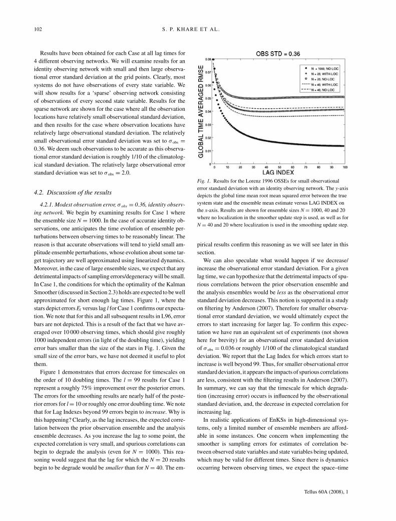
approximated for short enough lag times. Figure 1, where the
stars depict errors El versus lag l for Case 1 confirms our expecta-
tion. We note that for this and all subsequent results in L96, error
bars are not depicted. This is a result of the fact that we have av-
eraged over 10 000 observing times, which should give roughly
1000 independent errors (in light of the doubling time), yielding
error bars smaller than the size of the stars in Fig. 1. Given the
small size of the error bars, we have not deemed it useful to plot
them.
Figure 1 demonstrates that errors decrease for timescales on
the order of 10 doubling times. The l = 99 results for Case 1
represent a roughly 75% improvement over the posterior errors.
The errors for the smoothing results are nearly half of the poste-
rior errors for l = 10 or roughly one error doubling time. We note
that for Lag Indexes beyond 99 errors begin to increase. Why is
this happening? Clearly, as the lag increases, the expected corre-
lation between the prior observation ensemble and the analysis
ensemble decreases. As you increase the lag to some point, the
expected correlation is very small, and spurious correlations can
begin to degrade the analysis (even for N = 1000). This rea-
soning would suggest that the lag for which the N = 20 results
begin to be degrade would be smaller than for N = 40. The em-
Fig. 1. Results for the Lorenz 1996 OSSEs for small observational
error standard deviation with an identity observing network. The y-axis
depicts the global time mean root mean squared error between the true
system state and the ensemble mean estimate versus LAG INDEX on
the x-axis. Results are shown for ensemble sizes N = 1000, 40 and 20
where no localization in the smoother update step is used, as well as for
N = 40 and 20 where localization is used in the smoothing update step.
pirical results confirm this reasoning as we will see later in this
section.
We can also speculate what would happen if we decrease/
increase the observational error standard deviation. For a given
lag time, we can hypothesize that the detrimental impacts of spu-
rious correlations between the prior observation ensemble and
the analysis ensembles would be less as the observational error
standard deviation decreases. This notion is supported in a study
on filtering by Anderson (2007). Therefore for smaller observa-
tional error standard deviation, we would ultimately expect the
errors to start increasing for larger lag. To confirm this expec-
tation we have run an equivalent set of experiments (not shown
here for brevity) for an observational error standard deviation
of σ obs = 0.036 or roughly 1/100 of the climatological standard
deviation. We report that the Lag Index for which errors start to
increase is well beyond 99. Thus, for smaller observational error
standard deviation, it appears the impacts of spurious correlations
are less, consistent with the filtering results in Anderson (2007).
In summary, we can say that the timescale for which degrada-
tion (increasing error) occurs is influenced by the observational
standard deviation, and, the decrease in expected correlation for
increasing lag.
In realistic applications of EnKSs in high-dimensional sys-
tems, only a limited number of ensemble members are afford-
able in some instances. One concern when implementing the
smoother is sampling errors for estimates of correlation be-
tween observed state variables and state variables being updated,
which may be valid for different times. Since there is dynamics
occurring between observing times, we expect the space–time
Tellus 60A (2008), 1
Page 7
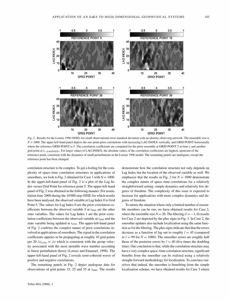
APPLICATION OF AN EnKS TO HIGH-DIMENSIONAL GEOPHYSICAL SYSTEMS 103
Fig. 2. Results for the Lorenz 1996 OSSEs for small observational error standard deviation with an identity observing network. The ensemble size is
N = 1000. The upper-left-hand panel depicts the one-point prior correlations with increasing LAG INDEX vertically, and GRID POINT horizontally
where the reference GRID POINT is 5. The correlation coefficients are computed for the prior ensemble at GRID POINT 5 at time ti and another
grid point at ti−(LAGINDEX). For larger values of LAG INDEX, the absolute values of the correlation coefficients are highest, upstream of the
reference point, consistent with the dynamics of small perturbations in the Lorenz 1996 model. The remaining panels are analogous, except the
reference point has been changed.
correlation structure to be complex. To get a feeling for the com-
plexity of space–time correlation structures in applications of
smoothers, we look to Fig. 2 obtained for Case 1 with N = 1000.
In the upper-left-hand panel of Fig. 2 is a plot of the Lag In-
dex versus Grid Point for reference point 5. The upper-left-hand
panel of Fig. 2 was obtained in the following manner: For assim-
ilation time 2000 during the 10 000 step OSSE for which results
have been analysed, the observed variable at Lag Index 0 is Grid
Point 5. The values for Lag Index 0 are the prior correlation co-
efficients between the observed variable 5 at t2000 are the other
state variables. The values for Lag Index 1 are the prior corre-
lation coefficients between the observed variable at t2000 and the
state variable being updated at t1999. The upper-left-hand panel
of Fig. 2 confirms the complex nature of prior correlations in-
volved in applications of smoothers. The signal in the correlation
coefficients appears to be propagating at roughly 10 grid points
per 20 �tassim = �t which is consistent with the group veloc-
ity associated with the most unstable wave number according
to linear perturbation theory (Lorenz and Emanuel, 1998). The
upper-left-hand panel of Fig. 2 reveals semi-coherent waves of
positive and negative correlations.
The remaining panels in Fig. 2 depict analogous data for
observations of grid points 15, 25 and 35 at t2000. The results
demonstrate how the correlation structure not only depends on
Lag Index but the location of the observed variable as well. We
emphasize that the results in Fig. 2 for N = 1000 demonstrate
the complex nature of space–time correlations for a relatively
straightforward setting: simple dynamics and relatively few de-
grees of freedom. The complexity of this issue is expected to
increase for applications with more complex dynamics and de-
grees of freedom.
To mimic the situation where only a limited number of ensem-
ble members can be run, we have obtained results for Case 2,
where the ensemble size N = 20. The filtering (l = −1, 0) results
for Case 2 are depicted by the plus signs in Fig. 1. In Case 2, the
smoother updates also include localization using the same func-
tion as for the filtering. The plus signs indicate that that the errors
decrease as a function of lag out to roughly l = 45 (compared
to l = 99 for N = 1000). The smoother errors are roughly half
those of the posterior errors by l = 40 (five times the doubling
time). Our conclusion is that, while the correlation structure may
have a very complex space–time correlation structure, significant
benefits from the smoother can be realized using a relatively
straight-forward methodology for localization. To convince our-
selves that indeed, the smoother is benefiting from the simple
localization scheme, we have obtained results for Case 3 where
Tellus 60A (2008), 1
Page 8
104 S . P. KHARE ET AL.
no covariance localization is used in the smoother updates. The
results in Fig. 1, indicated by the circles, clearly demonstrate the
benefit of using covariance localization in the smoother imple-
mentation. Note that the filtering results for Case 2 and 3 are
identical as they should be (again, the only distinction is the lo-
calization in the smoother updates). These results demonstrate
that covariance localization is crucial to realizing the full benefits
of the EnKS. It is possible that more general implementations of
covariance localization could yield improved results over Fig. 1.
One possibility is the group filter method of Anderson (2007).
While extensive investigation of this issue is beyond the scope
of this paper, our results for Case 2 set a benchmark for which
more general schemes should beat.
We now examine results for an intermediate ensemble size of
N = 40, corresponding to Case 4 where localization is used in
the smoother updates, and Case 5 where localization is not used
in the smoother updates. Figure 1 shows that the errors for Case
4 are lower than the errors for Case 2. Again, the only distinction
between Case 4 and Case 2 is the ensemble size. We also see
that the lag time for which the errors in Case 2 start increasing
is well before the lag time for which this happens in Case 4.
Our suggestion is that spurious correlations between the prior
observation ensemble and the analysis ensemble are degrading
the performance of the smoother for high lag index. Again, the
rationale is that the N = 40 ensemble is less impacted by spurious
correlations which are likely to arise as lag increases (and the
expected correlation goes down). We note that the N = 40 no
localization results of Case 5 are generally worse than Case 2
(N = 20 with localization). This bolsters the importance of using
localization in ensemble smoother implementations. Finally, we
can compare Case 3 (N = 20) and Case 5 (N = 40) where no
localizations are used in the smoother updates. Consistent with
our previous reasoning, the errors for the N = 20 case start to
rise at a smaller lag than for N = 40.
4.2.2. Large observation error, σ obs = 2.0, identity observingnetwork. In Fig. 3, results for Cases 1–5 are shown for experi-
ments where the observational standard deviation was set to 2.0.
For Case 1 with ensemble size N = 1000, the Lag Index at which
the errors begin to increase is roughly l = 70, whereas in the small
observational error size case (Fig. 1) the errors begin to increase
at l = 99. This again, supports the previously discussed notion
that in the larger observation error case, the impacts of spurious
correlations are more severe. Once again, we note that this is
consistent with the findings in Anderson (2007) in a study of en-
semble filtering. We have confirmed that the larger observation
error case is associated with larger analysis spread in comparison
to the small observation error case. For example, the time and
spatial mean ensemble spread for lags 1, 20, 80 are 0.325, 0.110,
0.025 for the N = 1000 large observation error case, where as
they are 0.047, 0.020, 0.005 for the N = 1000 small observation
error case. The finding that the smaller observation error case
has a longer optimal timescale has a complementary explana-
tion. Less accurate observations have less information content.
Fig. 3. Results for the Lorenz 1996 OSSEs for large observational
error standard deviation with an identity observing network. The y-axis
depicts the global time mean root mean squared error between the true
system state and the ensemble mean estimate versus LAG INDEX on
the x-axis. Results are shown for ensemble sizes N = 1000, 40 and 20
where no localization in the smoother update step is used, as well as for
N = 40 and 20 where localization is used in the smoothing update step.
For the large observation error case, we expect that as the analysis
variance decreases with increasing lag, the impact of observa-
tions becomes negligible, because the ratio of analysis variance
to observational error variance decreases.
For Case 1 in Fig. 3, we note that the percentage improvement
for the lowest value of El=70 with respect to the posterior errors
(El=0) is roughly 50%, less of a relative improvement than in
Fig. 1. In the smaller observation error case (Fig. 1), due to
smaller ensemble spread, the evolution of ensemble perturba-
tions between observing times is better approximated by lin-
earized dynamics. Hence, the linearity assumptions inherent to
the EnKS are less violated than in Fig. 3. This is one way of
reasoning why, for Case 1, the relative improvement is higher in
Fig. 1 than in Fig. 3.
Figure 3 also depicts results for the N = 20 results of Case 2
and Case 3. Much like the small observational error case, condi-
tioning on future observations once again improves our estimate
of the true state. As for the results in Fig. 1, we note the impact
of covariance localization for the state estimates obtained by the
smoother (Case 2 versus Case 3). The analogous one-point cor-
relation maps for the large observational error case once again
reveal the complex nature of the space–time prior correlation
structure (results not shown for brevity). As for the small obser-
vational error case, our expectation is that more general imple-
mentations of covariance localization may improve the results
for Case 2 depicted in Fig. 3.
The comparison of the N = 40 results with the N = 20 results
is similar to the small observation error size case. For example,
comparing Case 3 and Case 5, we see that the lag for which
Tellus 60A (2008), 1
Page 9
APPLICATION OF AN EnKS TO HIGH-DIMENSIONAL GEOPHYSICAL SYSTEMS 105
Fig. 4. Results for the Lorenz 1996 OSSEs for small observational
error standard deviation with a ‘SPARSE’ observing network which
consists of observations of every second state variable. The y-axis
depicts the global time mean root mean squared error between the true
system state and the ensemble mean estimate versus LAG INDEX on
the x-axis. Results are shown for ensemble sizes N = 1000, 40 and 20
where no localization in the smoother update step is used, as well as for
N = 40, 20 where localization is used in the smoothing update step.
errors start increasing in Case 5 is larger than for Case 3. This
again follows the rationale that the larger ensemble size results
are less impacted by spurious correlations.
4.2.3. Results for the ‘sparse’ observing networks. Figures 4
and 5 depict results for the sparse observing network for the
modest and large observation error sizes, respectively. By care-
fully comparing Figs. 1 and 3 with Figs. 4 and 5, we can see
that many of the relationships between the Cases are preserved.
Interestingly, the sparse network results demonstrate that much
of the reasoning applied to the identity observations case applies
to the sparse case.
5. Demonstration of an EnKS in an atmosphericGCM
5.1. Model description and the cases examined
The model is a numerical solution of the primitive equations for-
mulated in sigma coordinates. The prognostic variables in the
atmospheric general circulation model (AGCM) are zonal wind
U, meridional wind V, temperature T and surface pressure PS.
The geopotential height equation is diagnostic (as a consequence
of hydrostatic balance). A thorough description of the particular
model used can be found in Khare (2004). Our intention was
to use a simplified model whose behaviour is qualitatively re-
lated to the observed atmosphere. The model that has been used
in our numerical experiments is the dynamic core used in the
GFDL global atmospheric model (Anderson et al., 2005, here-
Fig. 5. Results for the Lorenz 1996 OSSEs for large observational
error standard deviation with a ‘SPARSE’ observing network which
consists of observations of every second state variable. The y-axis
depicts the global time mean root mean squared error between the true
system state and the ensemble mean estimate versus LAG INDEX on
the x-axis. Results are shown for ensemble sizes N = 1000, 40 and 20
where no localization in the smoother update step is used, as well as for
N = 40 and 20 where localization is used in the smoothing update step.
after A05), using a forcing and dissipation suggested by Held
and Suarez (1994). The forcing is a Newtonian relaxation to-
wards a zonally symmetric state without any daily or seasonal
cycle. The form of the forcing is equivalent in the northern and
southern hemispheres. In both hemispheres, the forcing drives a
pole to equator temperature gradient. A simple Rayleigh damp-
ing is used near the surface for dissipation. The model has no
topography, landmasses or parametrizations of subgrid scale pro-
cesses. The forcing used in this model can be thought of as a re-
placement for detailed radiative, turbulence and moist convective
parametrizations (Held and Suarez, 1994).
Numerical integration of this model is done using a B-grid
discretization and a vertical discretization described in Simmons
and Burridge (1981). The model consists of grid points spaced
6◦ apart in both latitude and longitude, respectively, with five
vertical levels. This B-grid discretization results in a total of
28 200 prognostic state variables. A model time step of 1 h was
used. This is approximately the minimum horizontal and vertical
resolution required to generate baroclinic instability with a time
mean climatology that is somewhat similar to the observed at-
mosphere (A05). A random sample of the model’s climatology
was obtained by making a 100 year integration of the AGCM
from a state of rest. The temperatures at the highest level of this
model equilibrate very slowly compared to all the other variables
(A05). It may take several years of integration for the highest
level temperatures to equilibrate, while it appears all other state
variables have equilibrated (A05). As a result, a 100 yr integra-
tion was used to obtain a state considered to be a random sample
Tellus 60A (2008), 1
Page 10
106 S . P. KHARE ET AL.
of the model’s climatology. This state was integrated an addi-
tional 4000 d. The initial true state was taken to be the model
state at the end of the 4000 d integration.
While the results for the L96 model demonstrate the ability of
the EnKS to improve state estimation by conditioning on obser-
vations valid at future times, it remains unclear whether or not the
algorithm can be applied successfully to high-dimensional pre-
diction problems. The numerical experiments in this Section ad-
dress this question by demonstrating the capabilities of the EnKS
in the high-dimensional AGCM described above for our chosen
experimental design. We now provide the relevant details of our
chosen experimental design. Numerical experiments with this
particular configuration of the AGCM indicate that the error dou-
bling time for the various dynamic variables at all model levels is
roughly 5 d, considerably slower than similar measures for state
of the art atmospheric prediction models. As a result, we choose
to assimilate observations every �tassim = 12 h. This roughly
mimics the ratio of doubling time to �tassim in current day oper-
ational systems (Bishop et al., 2003). We have chosen to demon-
strate the EnKS for an observational network consisting of 100
arbitrarily located column observations on the sphere (the ob-
servation operator uses horizontal bilinear interpolation). The
locations of the column observations are depicted in Fig. 6. The
locations of the column observations look somewhat irregular
with large data voids, not entirely unlike the earth’s radiosonde
network. Observational error standard deviations for PS, T, Uand V were set to 1 mb, 1 K, 1 m s−1 and 1 m s−1, respectively.
Cases B1 to B3 will be examined (B indicates B-grid to dis-
tinguish the cases from the L96 results). In Cases B1 and B2,
Fig. 6. A depiction of the observing system used in the OSSEs with the
Atmospheric General Circulation Model in Section 5. Column
observations of the model’s dynamic variables (U, V, T and PS) are
located at centre of the crosses. There are 100 arbitrarily chosen
column observations in total. Column observations are simulated every
12 h at the locations depicted. Horizontal bilinear interpolation was
used in the observation operator.
ensemble sizes of N = 20 were used, whereas in Case B3,
N = 50 was used. For the Gaspari–Cohn function used for co-
variance localization, distance between two grid points is de-
fined as the horizontal distance along the sphere expressed in
radians. No localization is used in the vertical. Cases B1 and
B3 use this Gaspari–Cohn localization in both the filtering and
smoother updates. A half-width of c = 0.25 radians and no co-
variance inflation was used, consistent with previous assimila-
tion studies in this model (Anderson et al., 2005; Khare and
Anderson, 2006b). While our use of constant c across the cases
is not optimal, it serves our intended purpose of isolating the
impacts of changing ensemble size. For Case B2, the same co-
variance localization for the filtering updates was used. For the
smoother updates in Case B2 no covariance localization was used
whatsoever.
5.2. Discussion of the results
Before moving onto our analysis of the lagged smoother results,
it is important to first ensure that the filter is working, and yielding
sensible answers. Figure 7 depicts results for Case B1. The upper-
left-hand panel of Fig. 7 depicts the fractional difference, as a
function of longitude and latitude, between the mean distance to
the truth for a free climatological run and posterior error results
obtained for Case B1. For a given PS grid point (for example),
let the time-mean difference between the truth and the mean of
a free-running (climatological) ensemble be α. The time mean
posterior error is β. At the PS grid point in question, the fractional
difference is defined as, (β − α)/α. The upper-left-hand panel of
Fig. 7 reveals that for all grid points, the fractional differences are
indeed negative. The gains from the assimilation of observations
varies spatially in a manner consistent with the configuration
of the observational network. We note again that the errors were
computed using averages over 5000 d of simulation time (10 000
assimilation times with �tassim = 12 h gives 5000 d). Given the
large number of samples, and hence the small size of error bars,
we deem it unnecessary to include error bars in Fig. 7 and any
subsequent plots. For the upper-left-hand panel of Fig. 7, we
note that maximal gains of nearly 85% have been achieved. The
remaining panels depict analogous results for mid-level T, Uand V. We have chosen to focus on the results in the mid-level
to avoid any concern of contaminating the results by the rather
severe numerical approximations that take place at the model
top. Qualitatively similar results were obtained for the N = 50
results in Case B3, not shown for brevity. Having checked that
we have obtained sensible filtering results, we no move onto
examine the lagged estimates.
We now focus our attention on the upper-left-hand panel of
Fig. 8, which displays globally averaged time mean RMSE errors
as a function of Lag Index (l) for PS. Results for Cases B1, B2
and B3 are depicted by the + signs, o’s and *’s, respectively. As
expected, the prior and posterior errors (l = −1, 0) are identical
for Case B1 and Case B2. In Case B1, globally averaged PS
Tellus 60A (2008), 1
Page 11
APPLICATION OF AN EnKS TO HIGH-DIMENSIONAL GEOPHYSICAL SYSTEMS 107
Fig. 7. The upper-left-hand panel depicts results for the surface pressure PS. At each model grid point, the fractional difference between the time
mean absolute posterior error in the OSSE and a free climatological run has been computed. The panels depict contour plots of the fractional
differences. The remaining panels depict results for the temperature T, zonal and meridional winds U and V.
Fig. 8. In the upper-left-hand panel are
results for PS from the OSSEs with the
Atmospheric General Circulation Model.
The vertical axis contains the global, time
mean, root mean squared difference between
the PS ensemble mean and truth. The o’s
depict results for ensemble size N = 20
without localization in the smoother update
step. The +’s and *’s depict results for N =20 and 50, where localization has been used
in the smoother update steps, respectively.
The upper-right-, lower-left- and
lower-right-hand panels depict the analogous
results for T, U and V, respectively.
errors decrease as a function of Lag Index out to l = 10 (twice the
estimated doubling time) beyond which errors start to increase.
The results for l = 10 result in roughly a 10% decrease in errors
compared to the posterior errors. 10% in this case is non-trivial
as we are averaging globally and the network can be considered
sparse. The results for Case B2 clearly demonstrate how crucial
a proper covariance localization scheme is to getting sensible
results from the EnKS. Given the results for case B2, we choose
Tellus 60A (2008), 1
Page 12
108 S . P. KHARE ET AL.
to focus the remainder of our attention on Cases B1 and B3,
where localization has been used in the smoother updates.
The N = 50 results for Case B3 generally yield lower globally
averaged errors (compared to the N = 20 results). The relative
improvement of the global errors in B3 is higher (20%) than in
B2. In Case B3, the errors decrease up to l=15, unlike the smaller
ensemble size results which appear to start increasing after
l = 10. Given our analysis in the low-order model, our rationale
for why the optimal timescale for Case B3 is longer, is that the
N = 50 ensemble is better able to handle the detrimental impacts
of sampling errors. Therefore, we draw a very encouraging con-
clusion that increasing the ensemble size in our GCM, allows one
to yield larger relative improvements in state estimation. Anal-
ogous results for T, U and V are depicted in the upper-right-,
lower-left- and lower-right-panels, respectively. Qualitatively
similar conclusions can be drawn in all cases.
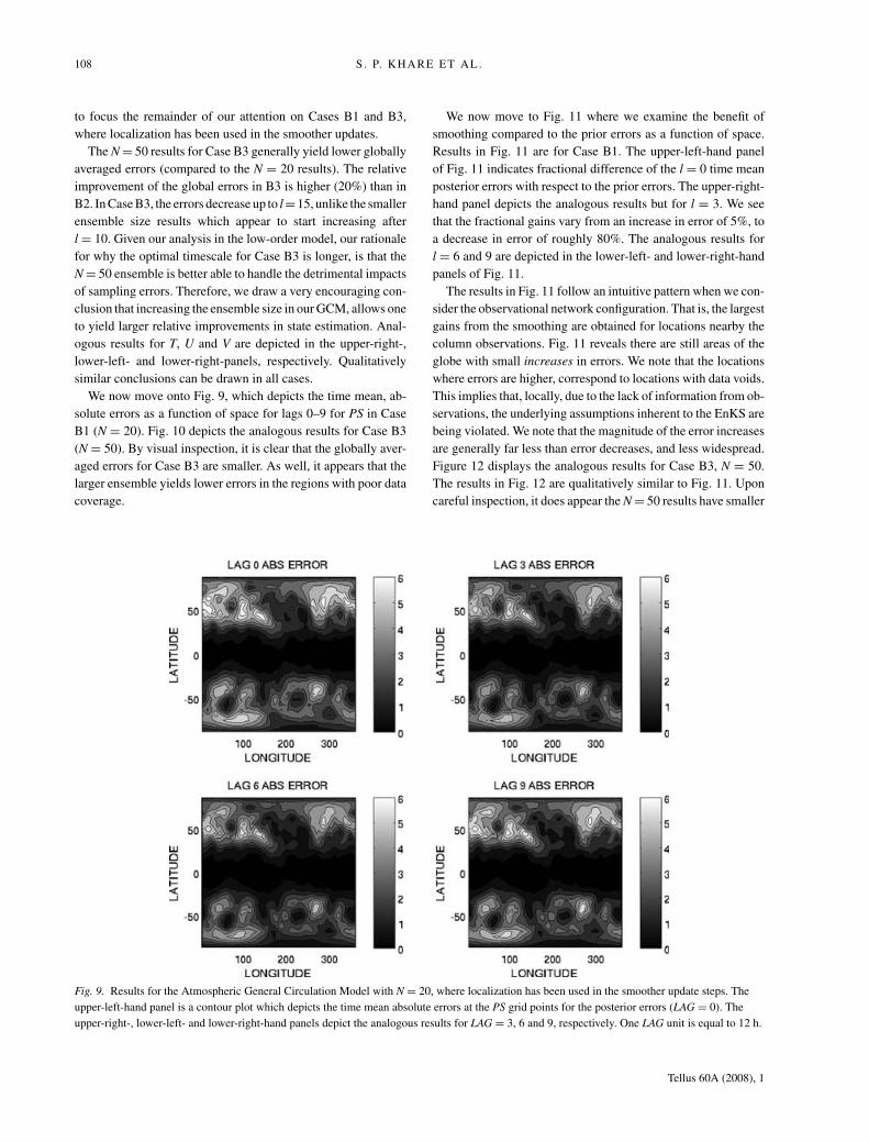
We now move onto Fig. 9, which depicts the time mean, ab-
solute errors as a function of space for lags 0–9 for PS in Case
B1 (N = 20). Fig. 10 depicts the analogous results for Case B3
(N = 50). By visual inspection, it is clear that the globally aver-
aged errors for Case B3 are smaller. As well, it appears that the
larger ensemble yields lower errors in the regions with poor data
coverage.
Fig. 9. Results for the Atmospheric General Circulation Model with N = 20, where localization has been used in the smoother update steps. The
upper-left-hand panel is a contour plot which depicts the time mean absolute errors at the PS grid points for the posterior errors (LAG = 0). The
upper-right-, lower-left- and lower-right-hand panels depict the analogous results for LAG = 3, 6 and 9, respectively. One LAG unit is equal to 12 h.
We now move to Fig. 11 where we examine the benefit of
smoothing compared to the prior errors as a function of space.
Results in Fig. 11 are for Case B1. The upper-left-hand panel
of Fig. 11 indicates fractional difference of the l = 0 time mean
posterior errors with respect to the prior errors. The upper-right-
hand panel depicts the analogous results but for l = 3. We see
that the fractional gains vary from an increase in error of 5%, to
a decrease in error of roughly 80%. The analogous results for
l = 6 and 9 are depicted in the lower-left- and lower-right-hand
panels of Fig. 11.
The results in Fig. 11 follow an intuitive pattern when we con-
sider the observational network configuration. That is, the largest
gains from the smoothing are obtained for locations nearby the
column observations. Fig. 11 reveals there are still areas of the
globe with small increases in errors. We note that the locations
where errors are higher, correspond to locations with data voids.
This implies that, locally, due to the lack of information from ob-
servations, the underlying assumptions inherent to the EnKS are
being violated. We note that the magnitude of the error increases
are generally far less than error decreases, and less widespread.
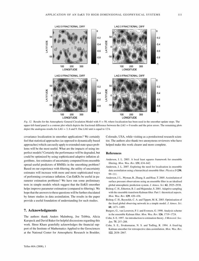
Figure 12 displays the analogous results for Case B3, N = 50.
The results in Fig. 12 are qualitatively similar to Fig. 11. Upon
careful inspection, it does appear the N = 50 results have smaller
Tellus 60A (2008), 1
Page 13
APPLICATION OF AN EnKS TO HIGH-DIMENSIONAL GEOPHYSICAL SYSTEMS 109
Fig. 10. Results for the Atmospheric General Circulation Model with N = 50, where localization has been used in the smoother update steps. The
upper-left-hand panel is a contour plot which depicts the time mean absolute errors at the PS grid points for the posterior errors (LAG = 0). The
upper-right-, lower-left- and lower-right-hand panels depict the analogous results for LAG = 3, 6 and 9, respectively. One LAG unit is equal to 12 h.
areas of error increases, which suggests the increases are due to
sampling errors.
6. Summary, conclusions and future work
The key goal of this paper is to demonstrate the application
of an EnKS to high-dimensional geophysical analysis prob-
lems. A review of the probabilistic framework underlying the
smoother is provided in Section 2, along with a discussion
of how the algorithm is implemented using a generic ensem-
ble Kalman filter update algorithm. The results in this study
were obtained using the perturbed observation EnKF using the
implementation described in Anderson (2003). To achieve our
goal, a series OSSEs in a set of dynamic systems have been
analysed.
In Section 4, results obtained from a 40-D non-linear Lorenz
1996 model were analysed. The following conclusions are drawn
from the Lorenz 1996 OSSEs:
(i) In a large ensemble, small observation error limit, with
an identity network, conditioning on future observations up to
10 error doubling times, yields ensemble mean state estimates
which are closer to truth on average. Conditioning on observa-
tions beyond an optimal timescale yields progressively worse
ensemble mean estimates of truth. The optimal timescale is de-
fined as the lag time which was found to achieve the smallest
mean squared error. Our rationale is that larger lag leads to lower
expected correlations between observed and analysed state vari-
ables, and hence spurious correlations for progressively longer
lag degrade analyses.
(ii) In a large ensemble, identity observations case, the opti-
mal timescale gets progressively longer as the observation error
size decreases. One rationale for this result is that the impacts
of spurious correlations are diminished as the observation error
size decreases. We have also found that smaller observation error
sizes are associated with smaller analysis spread.
(iii) In a large ensemble size, identity observations case, the
relative improvement of using the smoother is larger in the small
observation error case. Our rationale for this is that in the small
observation error case, the evolution of ensemble perturbations
between observing times is better approximated by linearized
dynamics, more in line with the assumptions inherent to the
EnKS.
(iv) The EnKS can be successfully implemented in Lorenz
1996 with an ensemble size of N = 20 with an identity observ-
ing network. We find that space–time covariance localization is
crucial to optimizing the performance of the EnKS for N = 20.
(v) Generally, the N = 40 results yield longer optimal
timescales than N = 20, which we attribute to smaller sampling
errors.
Tellus 60A (2008), 1
Page 14
110 S . P. KHARE ET AL.
Fig. 11. Results for the Atmospheric General Circulation Model with N = 20, where localization has been used in the smoother update steps. The
upper-left-hand panel is a contour plot which depicts the fractional difference between the LAG = 0 results and the prior errors. The remaining plots
depict the analogous results for LAG = 3, 6 and 9. One LAG unit is equal to 12 h.
(vi) Qualitatively similar conclusions have been drawn for
analogous experiments with a sparse observing network.
In Section 5, we have successfully demonstrated the use of
an EnKS in an atmospheric GCM for an observing network
comprised of 100 arbitrarily located column observations on the
sphere. We draw the following conclusions from these results:
(i) The use of an EnKS can reduce time mean RMSE er-
rors for implementations with small ensemble sizes in high-
dimensional prediction models.
(ii) The relative benefit of using the EnKS appears higher
as the ensemble size increases. Based on our results from the
low-order model, our rationale is that this can be attributed to
the larger ensembles’ ability to reduce sampling errors.
(iii) For an ensemble size of N = 20, a 10% decrease in glob-
ally averaged errors was achieved. This was deemed to be non-
trivial due to the sparsity of the observation network. For N =50, an even more encouraging 20% reduction in global errors
was achieved.
(iv) Gains of roughly 30% over posterior errors were obtained
in locations nearby observations.
(v) When updating ensembles of state estimates valid at a
given time, with observations valid at future times, covariance lo-
calization is critical to achieving sensible results from the EnKS
when using small ensemble sizes in high-dimensional prediction
systems.
We have demonstrated that the EnKS can be successfully ap-
plied when assimilating observations in a high-dimensional pre-
diction system. In light of these results, the prospect of using
the EnKSs in real applications is exciting indeed. We note that
the current day NCEP and ECMWF reanalyses use up to date
prediction models and data assimilation systems to generate es-
timates of the atmospheric state over a long time window in the
past (e.g. Kalnay et al., 1996; Simmons and Gibson, 2000). Cohn
et al. (1994) discuss how the NCEP and ECMWF systems do
not make use of the full record of observations. The results in
this paper, albeit in a perfect model setting, clearly demonstrate
the benefits of conditioning on future observations to achieve
more accurate state estimation. Given the results for the GCM,
we emphasize that these benefits can be achieved, even when
using small ensemble sizes in high-dimensional prediction sys-
tems. From a practical point of view, the EnKS is a very attractive
means of conditioning on future observations as the algorithm
can be applied without having to compute model or observation
operator linearizations which is a time-consuming and complex
procedure.
This study brings forth a number of interesting research ques-
tions upon which we can speculate: What is the best method for
Tellus 60A (2008), 1
Page 15
APPLICATION OF AN EnKS TO HIGH-DIMENSIONAL GEOPHYSICAL SYSTEMS 111
Fig. 12. Results for the Atmospheric General Circulation Model with N = 50, where localization has been used in the smoother update steps. The
upper-left-hand panel is a contour plot which depicts the fractional difference between the LAG = 0 results and the prior errors. The remaining plots
depict the analogous results for LAG = 3, 6 and 9. One LAG unit is equal to 12 h.
covariance localization in smoother applications? We certainly
feel that statistical approaches (as opposed to dynamically based
approaches) which can easily apply to extended state space prob-
lems will be the most useful. What are the impacts of using im-
perfect models? Certainly the performance will be degraded, but
could be optimized by using sophisticated adaptive inflation al-
gorithms. Are estimates of uncertainty computed from ensemble
spread useful predictors of RMSEs in the smoothing problem?
Based on our experience with filtering, the utility of uncertainty
estimates will increase with more and more sophisticated ways
of performing covariance inflation. Can EnKSs be useful in pa-
rameter estimation problems? We have run some preliminary
tests in simple models which suggest that the EnKS smoother
helps improve parameter estimation (compared to filtering). We
hope that the answers to these questions will be further elucidated
by future studies in data assimilation. The results in the paper
provide a useful foundation of understanding for such studies.
7. Acknowledgments
The authors thank Anders Malmberg, Joe Tribbia, Alicia
Karspeck and David Baker for helpful discussions regarding this
work. Shree Khare gratefully acknowledges the financial sup-
port of the Institute of Mathematics Applied to the Geosciences
at the National Center for Atmospheric Research in Boulder,
Colorado, USA, while visiting as a postdoctoral research scien-
tist. The authors also thank two anonymous reviewers who have
helped make this work clearer and more complete.
References
Anderson, J. L. 2003. A local least squares framework for ensemble
filtering. Mon. Wea. Rev. 131, 634–642.
Anderson, J. L. 2007. Exploring the need for localisation in ensemble
data assimilation using a hierarchical ensemble filter. Physica D 230,
99–111.
Anderson, J. L., Wyman, B., Zhang, S. and Hoar, T. 2005. Assimilation of
surface pressure observations using an ensemble filter in an idealised
global atmospheric prediction system. J. Atmos. Sci. 62, 2925–2938.
Bishop, C. H., Etherton, B. J. and Majumdar, S. 2001. Adaptive sampling
with the ensemble transform Kalman filter. Part 1: theoretical aspects.
Mon. Wea. Rev. 129, 420–436.
Bishop, C. H., Reynolds, C. A. and Tippett, M. K. 2003. Optimisation of
the fixed global observing network in a simple model. J. Atmos. Sci.60, 1471–1489.
Burgers, G., van Leeuwen, P. J. and Evensen, G. 1998. Analysis scheme
in the ensemble Kalman filter. Mon. Wea. Rev. 126, 1719–1724.
Cohn, S. E. 1997. An introduction to estimation theory. J Meteorol. Soc.Jpn. 75, 257–288.
Cohn, S. E., Sivakumaran, N. S. and Todling, R. 1994. A fixed-lag
Kalman smoother for retrospective data assimilation. Mon. Wea. Rev.122, 2838–2867.
Tellus 60A (2008), 1
Page 16
112 S . P. KHARE ET AL.
Daley, R. 1991. Atmospheric Data Analysis. Vol. 2. Cambridge Univer-
sity Press, New York, 457 pp.
Evensen, G. 1994. Sequential data assimilation with a nonlinear quasi-
geostrophic model using Monte Carlo methods to forecast error statis-
tics. J. Geophys. Res. 99, 10143–10162.
Evensen, G. and van Leeuwen, P. J. 2000. An ensemble Kalman smoother
for nonlinear dynamics. Mon. Wea. Rev. 128, 1852–1867.
Evensen, G. 2003. The ensemble Kalman filter: theoretical formulation
and practical implementation. Ocean Dyn. 53, 343–367.
Gaspari, G. and Cohn, S. E. 1999. Construction of correlation functions
in two and three dimensions, J. R. Meteorol. Soc. 125, 723–757.
Hamill, T. M. and Snyder, C. 2001. Using improved background error
covariances from an ensemble Kalman filter for adaptive observations.
Mon. Wea. Rev. 130, 1552–1572.
Held, I. and Suarez, M. J. 1994. A proposal for the intercomparison of
the dynamical cores of atmospheric general circulation models. Bull.Am. Meteorol. Soc. 75, 1825–1830.
Houtekamer, P. L. and Mitchell, H. L. 1998. Data assimilation using
an ensemble Kalman filter technique. Mon. Wea. Rev. 126, 796–
811.
Houtekamer, P. L. and Mitchell, H. L. 2005. Atmospheric data assimi-
lation with an ensemble Kalman filter: results with real observations.
Mon. Wea. Rev. 133, 604–620.
Jazwinski, A. H. 1970. Stochastic Processes and Filtering Theory. Aca-
demic Press, San Diego, 376 pp.
Kalman, R. E. 1960. A new approach to linear filtering and prediction
problems. Trans. AMSE Ser. D. J. Basic. Eng. 82, 35–45.
Kalnay, E., Kanamitsu, M., Kistler, R., Collins, W., Deaven, D. and co-
authors, 1996. The NCEP/NCAR reanalysis project. Bull. Am. Mete-orol. Soc. 77, 437–471.
Khare, S. P. 2004. Observing Network Design for Improved Predictionof Geophysical Fluid Flows—Analysis of Ensemble Methods. PhD
thesis, Princeton University, 195 pp.
Khare, S. P. and Anderson, J. L. 2006a. An examination of ensemble filter
based adaptive observation methodologies. Tellus 58A, 179–195.
Khare, S. P. and Anderson, J. L. 2006b. A methodology for fixed obser-
vational network design: theory and application to a simulated global
prediction system. Tellus 58A, 523–537.
Lorenz, E. N. and Emanuel, K. A. 1998. Optimal sites for supplementary
weather observations: simulation with a small model, J. Atmos. Sci.55, 399–414.
Lorenz, E. N. 1996. Predictability: a problem partly solve. Proceedingsof the Seminar on Predictability Volume 1, ECMWF, Reading, Berk-
shire, UK, pp. 1–18.
Simmons, A. J. and Burridge, D. M. 1981. An energy and angular-
momentum conserving vertical finite-difference scheme and hybrid
vertical coordinates. Mon. Wea. Rev. 109, 758–766.
Simmons, A. J. and Gibson, J. K. 2000. ERA-40 Project report series
no. 1. The ERA-40 project plan, ECMWF, Reading, UK.
Snyder, C. and Zhang, F. 2003. Assimilation of simulated doppler radar
observations with an ensemble Kalman filter. Mon. Wea. Rev. 131,
1663–1667.
Tippett, M. K., Anderson, J. L., Bishop, C. H., Hamill, T. M. and
Whitaker, J. S. 2003. Ensemble square-root filters. Mon. Wea. Rev.
131, 1485–1490.
Whitaker, J. S. and Compo, G. P. 2002. An ensemble Kalman smoother
for reanalysis. Proc. Symp. on Observations, Data Assimilation andProbabilistic Prediction, Orlando, FL, Amer. Meteor. Soc., 144–147.
Whitaker, J. S. and Hamill, T. M. 2002. Ensemble data assimilation
without perturbed observations. Mon. Wea. Rev. 130, 1931–1924.
Tellus 60A (2008), 1