MEMPSODE: An Empirical Assessment of Local Search Algorithm Impact on a Memetic Algorithm Using Noiseless Testbed Costas Voglis * Department of Computer Science University of Ioannina GR-45110 Ioannina, Greece [email protected]Grigoris S. Piperagkas Department of Computer Science University of Ioannina GR-45110 Ioannina, Greece [email protected]Konstantinos E. Parsopoulos Department of Computer Science University of Ioannina GR-45110 Ioannina, Greece [email protected]Dimitris G. Papageorgiou Department of Materials Science and Engineering University of Ioannina GR-45110 Ioannina, Greece [email protected]Isaac E. Lagaris Department of Computer Science University of Ioannina GR-45110 Ioannina, Greece [email protected]ABSTRACT Memetic algorithms are hybrid schemes that usually inte- grate metaheuristics with classical local search techniques, in order to attain more balanced intensification/diversification trade–off in the search procedure. MEMPSODE is a recently published software that implements such memetic schemes, based on the Particle Swarm Optimization and Differential Evolution algorithms, as well as on the Merlin optimiza- tion environment that offers a variety of local search meth- ods. The present study aims at investigating the impact of the selected local search algorithm in the memetic schemes produced by MEMPSODE. Our interest was focused on gradient–free local search methods. We applied the derived memetic schemes on the noiseless testbed of the Black–Box Optimization Benchmarking 2012 workshop. The obtained results can offer significant insight to optimization practi- tioners with respect to the most promising approaches. Categories and Subject Descriptors G.1.6 [Numerical Analysis]: Optimization—global opti- mization ; G.4 [Mathematical Software] Keywords Global optimization, memetic algorithms, hybrid algorithms, Black–box optimization, local search * Corresponding author. Permission to make digital or hard copies of all or part of this work for personal or classroom use is granted without fee provided that copies are not made or distributed for profit or commercial advantage and that copies bear this notice and the full citation on the first page. To copy otherwise, to republish, to post on servers or to redistribute to lists, requires prior specific permission and/or a fee. GECCO’12 Companion, July 7–11, 2012, Philadelphia, PA, USA. Copyright 2012 ACM 978-1-4503-1178-6/12/07 ...$10.00. 1. INTRODUCTION Memetic Algorithms (MAs) are the outcome of integrat- ing metaheuristics with local search (LS) procedures. The combination of the two approaches is accompanied by in- creased effectiveness and accuracy for locating solutions of global optimization problems [5, 11]. The most common MA scheme assumes an evolving popu- lation and periodically applies LS to some or all its members. The dynamic of the MA is dictated by the choices of the user with respect to the following issues, also referred to as the fundamental memetic questions [11]: (I) Where will the LS procedures be applied. The user shall define the individuals that will constitute initial points for the LS. (II) When will the LS procedures be applied. The appli- cation frequency of LS shall be determined in order to attain a balanced exploitation of the available compu- tational budget. (III) How much of the computational budget will be con- sumed at each application of LS. The user must spec- ify the fraction of the available computational budget that will be devoted to LS. These issues were studied in [12], under a memetic strategy based on the Particle Swarm Optimization (PSO) algorithm. MEMPSODE (MEMetic Particle Swarm Optimization and Differential Evolution) is a recently introduced [16] software package that implements closely the PSO–based memetic approaches of [12] and extends them also to the Differential Evolution (DE) framework [14]. More specifically, MEMP- SODE contains implementations of the Unified PSO (UPSO) approach [10], which generalizes plain PSO by harnessing the strengths of its standard local and global variants, as well as the five basic DE operators. Also, MEMPSODE borrows LS methods from the Merlin optimization environment [9], which offers some of the most fundamental gradient–based and gradient–free LS methods. 245
Transcript
MEMPSODE: An Empirical Assessment of Local SearchAlgorithm Impact on a Memetic Algorithm
ABSTRACTMemetic algorithms are hybrid schemes that usually inte-grate metaheuristics with classical local search techniques, inorder to attain more balanced intensification/diversificationtrade–off in the search procedure. MEMPSODE is a recentlypublished software that implements such memetic schemes,based on the Particle Swarm Optimization and DifferentialEvolution algorithms, as well as on the Merlin optimiza-tion environment that offers a variety of local search meth-ods. The present study aims at investigating the impact ofthe selected local search algorithm in the memetic schemesproduced by MEMPSODE. Our interest was focused ongradient–free local search methods. We applied the derivedmemetic schemes on the noiseless testbed of the Black–BoxOptimization Benchmarking 2012 workshop. The obtainedresults can offer significant insight to optimization practi-tioners with respect to the most promising approaches.
KeywordsGlobal optimization, memetic algorithms, hybrid algorithms,Black–box optimization, local search
∗Corresponding author.
Permission to make digital or hard copies of all or part of this work forpersonal or classroom use is granted without fee provided that copies arenot made or distributed for profit or commercial advantage and that copiesbear this notice and the full citation on the first page. To copy otherwise, torepublish, to post on servers or to redistribute to lists, requires prior specificpermission and/or a fee.GECCO’12 Companion, July 7–11, 2012, Philadelphia, PA, USA.Copyright 2012 ACM 978-1-4503-1178-6/12/07 ...$10.00.
1. INTRODUCTIONMemetic Algorithms (MAs) are the outcome of integrat-
ing metaheuristics with local search (LS) procedures. Thecombination of the two approaches is accompanied by in-creased effectiveness and accuracy for locating solutions ofglobal optimization problems [5, 11].
The most common MA scheme assumes an evolving popu-lation and periodically applies LS to some or all its members.The dynamic of the MA is dictated by the choices of the userwith respect to the following issues, also referred to as thefundamental memetic questions [11]:
(I) Where will the LS procedures be applied. The usershall define the individuals that will constitute initialpoints for the LS.
(II) When will the LS procedures be applied. The appli-cation frequency of LS shall be determined in order toattain a balanced exploitation of the available compu-tational budget.
(III) How much of the computational budget will be con-sumed at each application of LS. The user must spec-ify the fraction of the available computational budgetthat will be devoted to LS.
These issues were studied in [12], under a memetic strategybased on the Particle Swarm Optimization (PSO) algorithm.
MEMPSODE (MEMetic Particle Swarm Optimization andDifferential Evolution) is a recently introduced [16] softwarepackage that implements closely the PSO–based memeticapproaches of [12] and extends them also to the DifferentialEvolution (DE) framework [14]. More specifically, MEMP-SODE contains implementations of the Unified PSO (UPSO)approach [10], which generalizes plain PSO by harnessingthe strengths of its standard local and global variants, as wellas the five basic DE operators. Also, MEMPSODE borrowsLS methods from the Merlin optimization environment [9],which offers some of the most fundamental gradient–basedand gradient–free LS methods.
245
Evidently, the choice of the LS scheme in an MA is ex-pected to have an impact on its performance. Attemptsto quantify this impact in hybrid evolutionary algorithms,were made in previous works. For instance, in [6] a hill–climbing method [13] was compared to the nonlinear sim-plex method [7] and CMA–ES [4]. Moreover, in [2] a hybridPSO was studied under the influence of the nonlinear sim-plex method [7] and Powell’s direction set method [8].
The present paper constitutes a first attempt to investi-gate the impact of the LS method on the MAs implementedin MEMPSODE. For this reason, we fixed the parameters ofall algorithms to specific values and alternated the LS pro-cedures combined with PSO and DE. The resulting memeticschemes were tested on the noiseless testbed of the Black–Box Optimization Benchmarking 2012 (BBOB’12) workshop.
The rest of the paper is organized as follows: the employedalgorithms are given in Section 2, while Section 3 describesthe experimental setting. The obtained experimental resultsare reported in Section 5, and the paper concludes in Sec-tion 6.
2. EMPLOYED ALGORITHMSThe design of the MA schemes presented in [12], were
based on PSO. In this context, the following three schemeswere proposed:
Scheme 1: LS is applied only on the overall best position,pg, of the swarm.
Scheme 2: LS is applied on each locally best position,pi, i = 1, 2, . . . , N , with a prescribed fixedprobability, ρ ∈ (0, 1].
Scheme 3: LS is applied both on the best position, pg,as well as on some randomly selected locallybest positions, pi, i ∈ {1, 2, . . . , N}.
These schemes can be applied either at each iteration orwhenever a specific number of consecutive iterations hasbeen completed.
In MEMPSODE [16] we extended this strategy to theDE [14] framework and incorporated the Merlin optimiza-tion environment for the LS procedures. A detailed presen-tation of the MEMPSODE software is provided in [16] aswell as in the accompanying manual of the software distri-bution.
A short description of the LS algorithms employed in thepresent work, are given in the following paragraphs. Thenotation used for the algorithms’ names, follows the corre-sponding MEMPSODE (Merlin) standard.
BFGS Method
BFGS belongs to the category of quasi–Newton methodswith line search [8]. At the start of k–th iteration a point
x(k), the gradient (or an finite–difference approximation)
g(k) and an approximation B(k) of the Hessian matrix areavailable. The method continues by performing a line search
to a direction s(k) defined as B(k)s(k) = −g(k), and anupdate from B(k) to B(k+1), using the BFGS update for-mula [1]. A careful selection of line search, in addition tothe powerful local properties of the Hessian approximation,results in one of the most robust and effective optimizationalgorithms.
TRUST Method
The TRUST method is a quasi–Newton algorithm that usesalso BFGS updates to maintain an approximation of theHessian, but for the step of the line search is properly se-lected to guarantee convergence, following the trust regionstrategy [8]. In this strategy, a quadratic model is being
build around the current point using the approximation B(k)
and the gradient vector g(k). The algorithm trusts only thequadratic model in a restricted region around the currentiterate. The restriction is usually imposed by a radius thatdefines a hypersphere.
SIMPLEX Method
This method belongs to the class of direct search methodsfor nonlinear optimization. It was designed by Nelder andMead [7]. The algorithm is based on the concept of simplex(or polytope) in Rn, which is a volume element defined by(n + 1) vertices. The input of the algorithm is an initialsimplex. The SIMPLEX algorithm then moves this initialsimplex towards the minimum by adapting its geometry andfinally shrinks it to a small volume element around the min-imizer. The procedure is derivative–free and proceeds to-wards the minimum using a set of n + 1 points. Thus, it isexpected to be tolerant to ill–conditioned cases. The trans-formation rules include contraction, expansion and shrinkageof the initial simplex.
ROLL Method
This method belongs to the class of pattern search meth-ods. It proceeds by taking proper steps along each coor-dinate direction, in turn. Then, the method performs anone–dimensional search on a properly formed direction, inorder to tackle possible correlations among the variables. Itsinput consists of the initial point and a user–defined explo-ration factor.
AUTO Method
AUTO is a procedure that tries to automatically select thebest LS algorithm. The methods BFGS, ROLL, SIMPLEXand TRUST are invoked one after the other. For each one, arate is calculated by dividing the relative achieved reductionof the function’s value by the number of function calls spent.The method with the highest rate is then invoked again andthe procedure is repeated. If all rates assume vanishing val-ues, then all the method tolerances are set to zero and themethods are applied in the following order: ROLL, TRUST,
BFGS, SIMPLEX.
3. EXPERIMENTAL SETUPWe used the default restart mechanism provided by the
noiseless testbed for a maximum number of 105 × n func-tion evaluations. The memetic Scheme 3 was used with LSprobability ρi = 0.05. We selected the default DE operatoras the main metaheuristic of the MA, with population sizeN = 25 and parameter values F = 0.5 and CR = 0.7.
Each LS application was restricted to 2000 function evalu-ations. Whenever first order derivatives were needed (e.g., inBFGS) we applied an O(h) finite–difference formula whereh is an adaptable step size [15]. The experiments were con-ducted on an Intel I7–2600 3.4 GHz processor machine with8GB RAM.
246
Dimension
Algorithm 2 3 5 10 20 40
BFGS 3.1−4 2.0−4 1.2−4 5.0−5 2.7−5 2.2−5
ROLL 4.6−5 5.4−5 5.7−5 5.6−5 4.5−5 3.8−5
SIMPLEX 2.1−4 1.5−4 9.2−5 5.1−5 5.5−5 5.7−5
AUTO 1.5−4 1.1−4 6.5−5 1.5−5 1.3−5 1.1−5
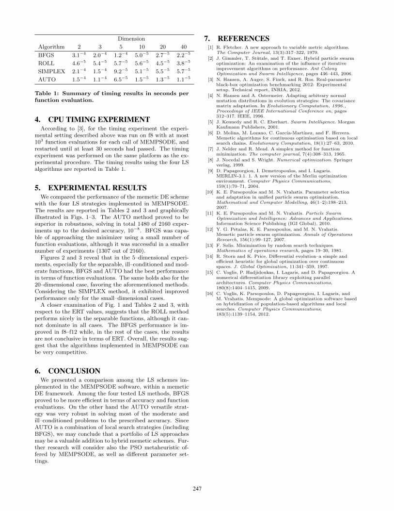
Table 1: Summary of timing results in seconds perfunction evaluation.
4. CPU TIMING EXPERIMENTAccording to [3], for the timing experiment the experi-
mental setting described above was run on f8 with at most103 function evaluations for each call of MEMPSODE, andrestarted until at least 30 seconds had passed. The timingexperiment was performed on the same platform as the ex-perimental procedure. The timing results using the four LSalgorithms are reported in Table 1.
5. EXPERIMENTAL RESULTSWe compared the performance of the memetic DE scheme
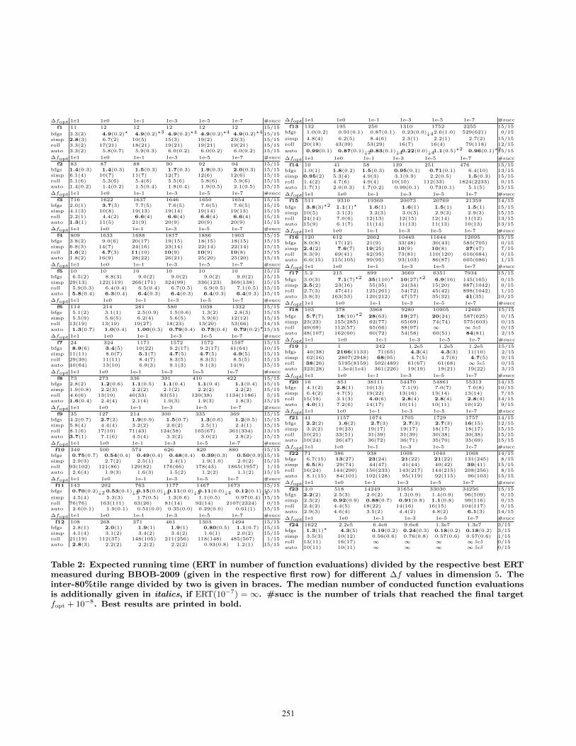
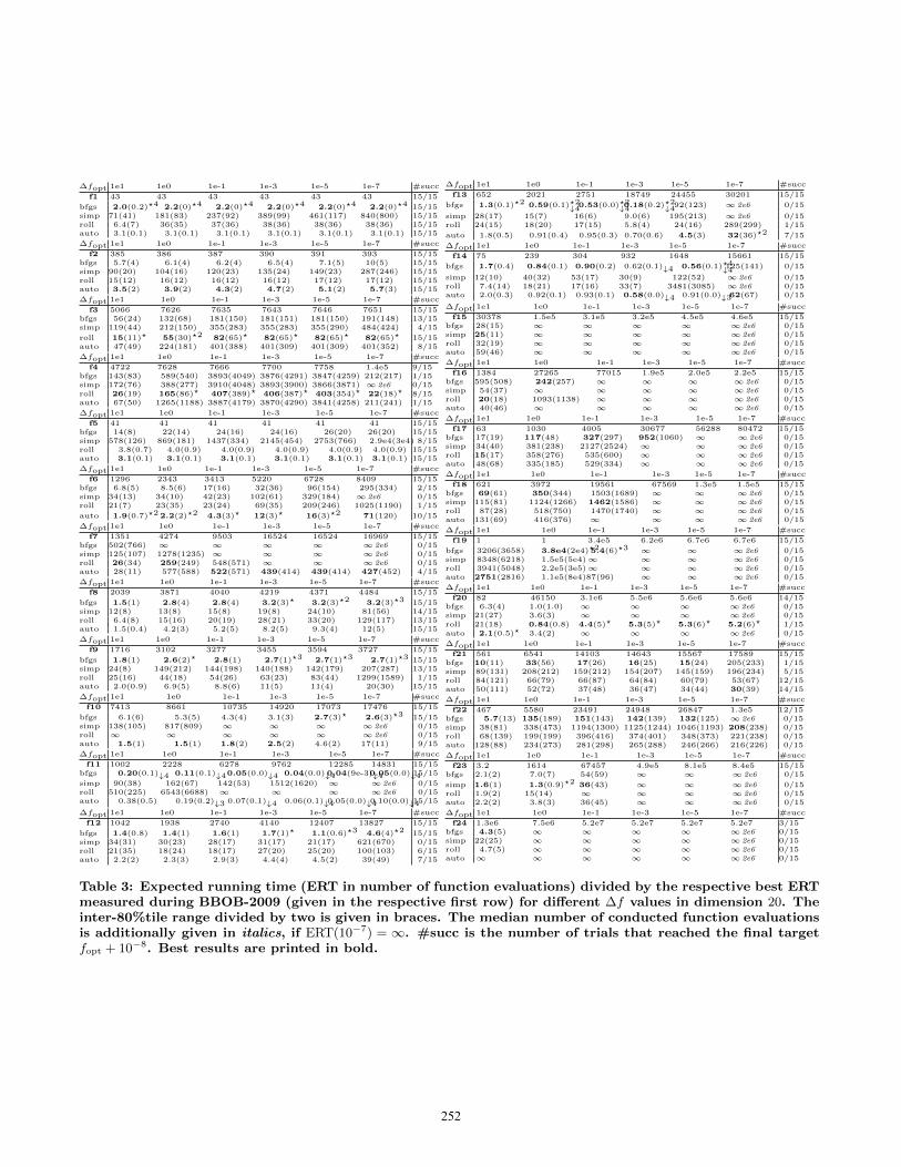
with the four LS strategies implemented in MEMPSODE.The results are reported in Tables 2 and 3 and graphicallyillustrated in Figs. 1–3. The AUTO method proved to besuperior in robustness, solving in total 1480 of 2160 exper-iments up to the desired accuracy, 10−8. BFGS was capa-ble of approaching the minimizer using a small number offunction evaluations, although it was successful in a smallernumber of experiments (1307 out of 2160).
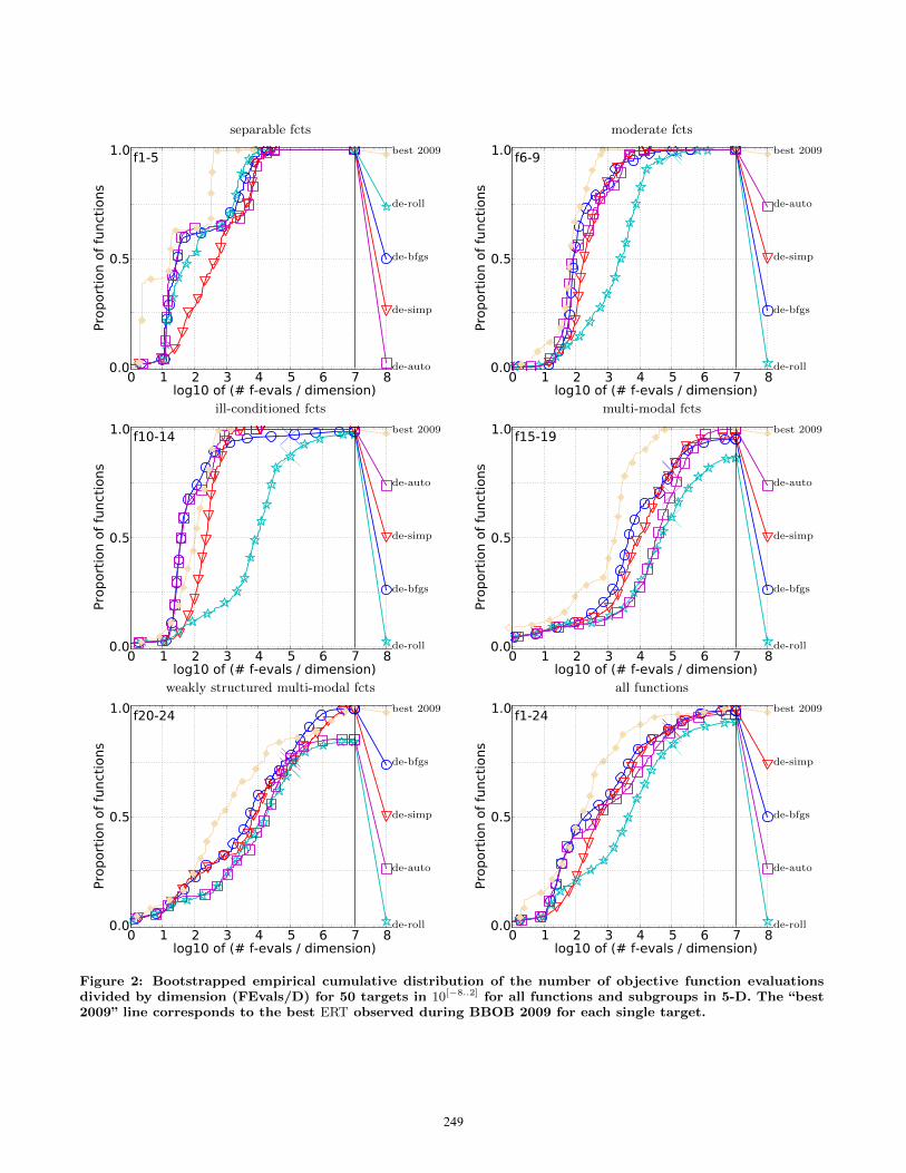
Figures 2 and 3 reveal that in the 5–dimensional experi-ments, especially for the separable, ill–conditioned and mod-erate functions, BFGS and AUTO had the best performancein terms of function evaluations. The same holds also for the20–dimensional case, favoring the aforementioned methods.Considering the SIMPLEX method, it exhibited improvedperformance only for the small–dimensional cases.
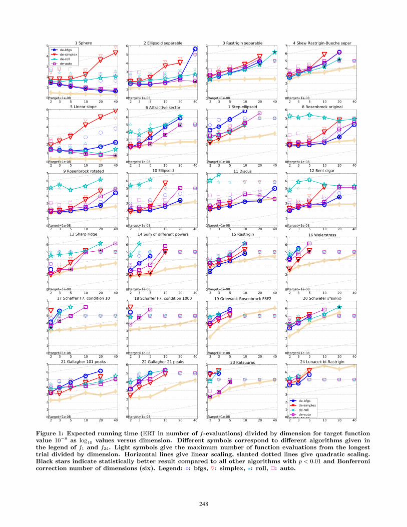
A closer examination of Fig. 1 and Tables 2 and 3, withrespect to the ERT values, suggests that the ROLL methodperforms nicely in the separable functions, although it can-not dominate in all cases. The BFGS performance is im-proved in f8–f12 while, in the rest of the cases, the resultsare not conclusive in terms of ERT. Overall, the results sug-gest that the algorithms implemented in MEMPSODE canbe very competitive.
6. CONCLUSIONWe presented a comparison among the LS schemes im-
plemented in the MEMPSODE software, within a memeticDE framework. Among the four tested LS methods, BFGSproved to be more efficient in terms of accuracy and functionevaluations. On the other hand the AUTO versatile strat-egy was very robust in solving most of the moderate andill–conditioned problems to the prescribed accuracy. SinceAUTO is a combination of local search strategies (includingBFGS), we may conclude that a portfolio of LS approachesmay be a valuable addition to hybrid memetic schemes. Fur-ther research will consider also the PSO metaheuristic of-fered by MEMPSODE, as well as different parameter set-tings.
7. REFERENCES[1] R. Fletcher. A new approach to variable metric algorithms.
The Computer Journal, 13(3):317–322, 1970.
[2] J. Gimmler, T. Stutzle, and T. Exner. Hybrid particle swarmoptimization: An examination of the influence of iterativeimprovement algorithms on performance. Ant ColonyOptimization and Swarm Intelligence, pages 436–443, 2006.
[3] N. Hansen, A. Auger, S. Finck, and R. Ros. Real-parameterblack-box optimization benchmarking 2012: Experimentalsetup. Technical report, INRIA, 2012.
[4] N. Hansen and A. Ostermeier. Adapting arbitrary normalmutation distributions in evolution strategies: The covariancematrix adaptation. In Evolutionary Computation, 1996.,Proceedings of IEEE International Conference on, pages312–317. IEEE, 1996.
[5] J. Kennedy and R. C. Eberhart. Swarm Intelligence. MorganKaufmann Publishers, 2001.
[6] D. Molina, M. Lozano, C. Garcıa-Martınez, and F. Herrera.Memetic algorithms for continuous optimisation based on localsearch chains. Evolutionary Computation, 18(1):27–63, 2010.
[7] J. Nelder and R. Mead. A simplex method for functionminimization. The computer journal, 7(4):308–313, 1965.
[8] J. Nocedal and S. Wright. Numerical optimization. Springerverlag, 1999.
[9] D. Papageorgiou, I. Demetropoulos, and I. Lagaris.MERLIN-3.1. 1. A new version of the Merlin optimizationenvironment. Computer Physics Communications,159(1):70–71, 2004.
[10] K. E. Parsopoulos and M. N. Vrahatis. Parameter selectionand adaptation in unified particle swarm optimization.Mathematical and Computer Modelling, 46(1–2):198–213,2007.
[11] K. E. Parsopoulos and M. N. Vrahatis. Particle SwarmOptimization and Intelligence: Advances and Applications.Information Science Publishing (IGI Global), 2010.
[12] Y. G. Petalas, K. E. Parsopoulos, and M. N. Vrahatis.Memetic particle swarm optimization. Annals of OperationsResearch, 156(1):99–127, 2007.
[13] F. Solis. Minimization by random search techniques.Mathematics of operations research, pages 19–30, 1981.
[14] R. Storn and K. Price. Differential evolution–a simple andefficient heuristic for global optimization over continuousspaces. J. Global Optimization, 11:341–359, 1997.
[15] C. Voglis, P. Hadjidoukas, I. Lagaris, and D. Papageorgiou. Anumerical differentiation library exploiting parallelarchitectures. Computer Physics Communications,180(8):1404–1415, 2009.
[16] C. Voglis, K. Parsopoulos, D. Papageorgiou, I. Lagaris, andM. Vrahatis. Mempsode: A global optimization software basedon hybridization of population-based algorithms and localsearches. Computer Physics Communications,183(5):1139–1154, 2012.
247
2 3 5 10 20 400
1
2
3
4
5
ftarget=1e-08
1 Spherede-bfgsde-simplexde-rollde-auto
2 3 5 10 20 400
1
2
3
4
5
6
ftarget=1e-08
2 Ellipsoid separable
2 3 5 10 20 400
1
2
3
4
5
6
7
ftarget=1e-08
3 Rastrigin separable
2 3 5 10 20 400
1
2
3
4
5
6
7
ftarget=1e-08
4 Skew Rastrigin-Bueche separ
2 3 5 10 20 400
1
2
3
4
5
6
ftarget=1e-08
5 Linear slope
2 3 5 10 20 400
1
2
3
4
5
6
7
ftarget=1e-08
6 Attractive sector
2 3 5 10 20 400
1
2
3
4
5
6
ftarget=1e-08
7 Step-ellipsoid
2 3 5 10 20 400
1
2
3
4
5
6
ftarget=1e-08
8 Rosenbrock original
2 3 5 10 20 400
1
2
3
4
5
6
7
ftarget=1e-08
9 Rosenbrock rotated
2 3 5 10 20 400
1
2
3
4
5
6
7
ftarget=1e-08
10 Ellipsoid
2 3 5 10 20 400
1
2
3
4
5
6
ftarget=1e-08
11 Discus
2 3 5 10 20 400
1
2
3
4
5
6
7
ftarget=1e-08
12 Bent cigar
2 3 5 10 20 400
1
2
3
4
5
6
7
ftarget=1e-08
13 Sharp ridge
2 3 5 10 20 400
1
2
3
4
5
6
7
ftarget=1e-08
14 Sum of different powers
2 3 5 10 20 400
1
2
3
4
5
6
7
ftarget=1e-08
15 Rastrigin
2 3 5 10 20 400
1
2
3
4
5
6
7
ftarget=1e-08
16 Weierstrass
2 3 5 10 20 400
1
2
3
4
5
6
7
ftarget=1e-08
17 Schaffer F7, condition 10
2 3 5 10 20 400
1
2
3
4
5
6
7
ftarget=1e-08
18 Schaffer F7, condition 1000
2 3 5 10 20 400
1
2
3
4
5
6
7
ftarget=1e-08
19 Griewank-Rosenbrock F8F2
2 3 5 10 20 400
1
2
3
4
5
6
7
ftarget=1e-08
20 Schwefel x*sin(x)
2 3 5 10 20 400
1
2
3
4
5
6
7
ftarget=1e-08
21 Gallagher 101 peaks
2 3 5 10 20 400
1
2
3
4
5
6
ftarget=1e-08
22 Gallagher 21 peaks
2 3 5 10 20 400
1
2
3
4
5
6
7
ftarget=1e-08
23 Katsuuras
2 3 5 10 20 400
1
2
3
4
5
6
7
ftarget=1e-08
24 Lunacek bi-Rastrigin
de-bfgsde-simplexde-rollde-auto
Figure 1: Expected running time (ERT in number of f-evaluations) divided by dimension for target functionvalue 10−8 as log10 values versus dimension. Different symbols correspond to different algorithms given inthe legend of f1 and f24. Light symbols give the maximum number of function evaluations from the longesttrial divided by dimension. Horizontal lines give linear scaling, slanted dotted lines give quadratic scaling.Black stars indicate statistically better result compared to all other algorithms with p < 0.01 and Bonferronicorrection number of dimensions (six). Legend: ◦: bfgs, O: simplex, ?: roll, 2: auto.
248
separable fcts moderate fcts
0 1 2 3 4 5 6 7 8log10 of (# f-evals / dimension)
0.0
0.5
1.0
Prop
ortio
n of
func
tions
de-auto
de-simplex
de-bfgs
de-roll
best 2009f1-5 best 2009
de-roll
de-bfgs
de-simp
de-auto0 1 2 3 4 5 6 7 8
log10 of (# f-evals / dimension)0.0
0.5
1.0
Prop
ortio
n of
func
tions
de-roll
de-bfgs
de-simplex
de-auto
best 2009f6-9 best 2009
de-auto
de-simp
de-bfgs
de-roll
ill-conditioned fcts multi-modal fcts
0 1 2 3 4 5 6 7 8log10 of (# f-evals / dimension)
0.0
0.5
1.0
Prop
ortio
n of
func
tions
de-roll
de-bfgs
de-simplex
de-auto
best 2009f10-14 best 2009
de-auto
de-simp
de-bfgs
de-roll0 1 2 3 4 5 6 7 8
log10 of (# f-evals / dimension)0.0
0.5
1.0
Prop
ortio
n of
func
tions
de-roll
de-bfgs
de-simplex
de-auto
best 2009f15-19 best 2009
de-auto
de-simp
de-bfgs
de-roll
weakly structured multi-modal fcts all functions
0 1 2 3 4 5 6 7 8log10 of (# f-evals / dimension)
0.0
0.5
1.0
Prop
ortio
n of
func
tions
de-roll
de-auto
de-simplex
de-bfgs
best 2009f20-24 best 2009
de-bfgs
de-simp
de-auto
de-roll0 1 2 3 4 5 6 7 8
log10 of (# f-evals / dimension)0.0
0.5
1.0
Prop
ortio
n of
func
tions
de-roll
de-auto
de-bfgs
de-simplex
best 2009f1-24 best 2009
de-simp
de-bfgs
de-auto
de-roll
Figure 2: Bootstrapped empirical cumulative distribution of the number of objective function evaluationsdivided by dimension (FEvals/D) for 50 targets in 10[−8..2] for all functions and subgroups in 5-D. The “best2009” line corresponds to the best ERT observed during BBOB 2009 for each single target.
249
separable fcts moderate fcts
0 1 2 3 4 5 6 7 8log10 of (# f-evals / dimension)
0.0
0.5
1.0
Prop
ortio
n of
func
tions
de-simplex
de-auto
de-bfgs
de-roll
best 2009f1-5 best 2009
de-roll
de-bfgs
de-auto
de-simp0 1 2 3 4 5 6 7 8
log10 of (# f-evals / dimension)0.0
0.5
1.0
Prop
ortio
n of
func
tions
de-simplex
de-bfgs
de-roll
de-auto
best 2009f6-9 best 2009
de-auto
de-roll
de-bfgs
de-simp
ill-conditioned fcts multi-modal fcts
0 1 2 3 4 5 6 7 8log10 of (# f-evals / dimension)
0.0
0.5
1.0
Prop
ortio
n of
func
tions
de-roll
de-simplex
de-bfgs
de-auto
best 2009f10-14 best 2009
de-auto
de-bfgs
de-simp
de-roll0 1 2 3 4 5 6 7 8
log10 of (# f-evals / dimension)0.0
0.5
1.0
Prop
ortio
n of
func
tions
de-auto
de-simplex
de-roll
de-bfgs
best 2009f15-19 best 2009
de-bfgs
de-roll
de-simp
de-auto
weakly structured multi-modal fcts all functions
0 1 2 3 4 5 6 7 8log10 of (# f-evals / dimension)
0.0
0.5
1.0
Prop
ortio
n of
func
tions
de-simplex
de-bfgs
de-auto
de-roll
best 2009f20-24 best 2009
de-roll
de-auto
de-bfgs
de-simp0 1 2 3 4 5 6 7 8
log10 of (# f-evals / dimension)0.0
0.5
1.0
Prop
ortio
n of
func
tions
de-simplex
de-roll
de-bfgs
de-auto
best 2009f1-24 best 2009
de-auto
de-bfgs
de-roll
de-simp
Figure 3: Bootstrapped empirical cumulative distribution of the number of objective function evaluationsdivided by dimension (FEvals/D) for 50 targets in 10[−8..2] for all functions and subgroups in 20-D. The “best2009” line corresponds to the best ERT observed during BBOB 2009 for each single target.
Table 2: Expected running time (ERT in number of function evaluations) divided by the respective best ERTmeasured during BBOB-2009 (given in the respective first row) for different ∆f values in dimension 5. Theinter-80%tile range divided by two is given in braces. The median number of conducted function evaluationsis additionally given in italics, if ERT(10−7) = ∞. #succ is the number of trials that reached the final targetfopt + 10−8. Best results are printed in bold.
Table 3: Expected running time (ERT in number of function evaluations) divided by the respective best ERTmeasured during BBOB-2009 (given in the respective first row) for different ∆f values in dimension 20. Theinter-80%tile range divided by two is given in braces. The median number of conducted function evaluationsis additionally given in italics, if ERT(10−7) = ∞. #succ is the number of trials that reached the final targetfopt + 10−8. Best results are printed in bold.