Mensch-Maschine-Interaktion 1

LMU München – Medieninformatik – Andreas Butz + Paul Holleis – Mensch-Maschine-Interaktion 1 – SS2010

Mensch-Maschine-Interaktion 1

Chapter 4 continued (June 10, 2010, 9am-12pm): User Study Statistics

1


Looking Back: User Study Design• Purpose of user studies• Placement within the development process• Types of user studies

– Observational, experimental– Within subjects, between groups

• Independent vs. dependent variables• Setup process

– Form hypotheses → design the study → run a pilot study → recruit participants → run the study → analyze the data

– Results must be valid, reliable, generalisable, important

2


User Study Design

• The Purpose of User Studies

• Research Aims: Reliability, Validity and Generalizability

• Research Methods and Experimental Designs

• Ethical Considerations

• HCI-related and practical information for your own studies

• Interpretation of Data and Presentation of Results

3


Types of Data• Nominal (categorical) data

– No relationship between the size of the number– Operations: A=B, A!=B– E.g. numbers in a football team

• Ordinal Data– Order / ranking– Operations: A>B, A<B, A=B– E.g. marks in school: 1, 2, 3, 4, 5, 6

• Interval scale data– Equal intervals = equal differences in the measured property– Zero point is arbitrary– E.g. temperature (°C/°F)

• Ratio scale data– Fixed zero point – E.g. wpm, error rates

usefulness

4


Types of Variables• Discrete Data

– Distinct and separate – Can be counted– E.g. Likert scales, preferences from a list, ...

• Continuous Data– Any value within a finite or infinite interval– Always have a order– E.g. weight, length, task completion time, ...

5

5-point Likert Scaleshttp://allpsych.com/researchmethods/images/likertscales.gif


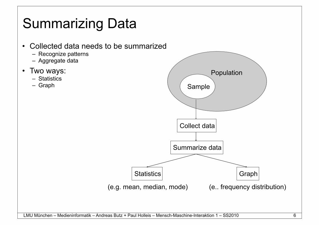
Summarizing Data• Collected data needs to be summarized

– Recognize patterns– Aggregate data

• Two ways:– Statistics– Graph Sample

Population

Collect data

Summarize data

Statistics Graph

(e.g. mean, median, mode) (e.. frequency distribution)

6


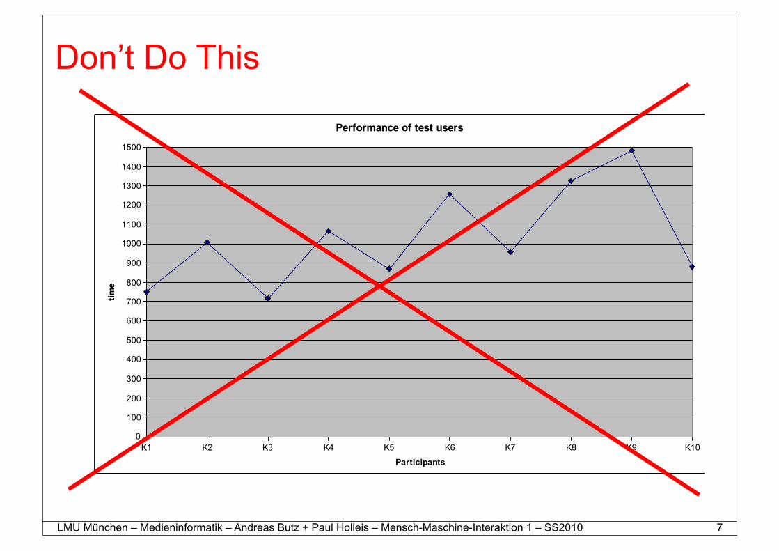
Don’t Do This

7


Frequency Distributions (Histograms)• Example: days needed to answer my email

Data: 5 2 2 3 4 4 3 2 0 3 0 3 2 1 5 1 3 1 5 5 2 4 0 0 4 5 4 4 5 5• Count the number of times each score occurs

Frequency table:

23%7520%6417%5317%5210%3113%40Frequency (%) Frequency Days

0

2

4

5

7

0 1 2 3 4 5

Histrogram

Freq

uenc

yScore

8


Averages: Mode, Median, Mean• How can the data be summed up in a single value? • Idea: get the centric point

• Three ways:– Mode

• The most frequent score– Median

• Middle score– Mean

• Average

9


Mode• The most frequent score• Describes how most people behave

• Pros:– Easy to calculate and understand– Can be used with nominal data

• Cons:– There can be more than one modes– Mode can change dramatically by adding only one dataset– Independent of all other data in the set mode

10


Median (Mdn)• Middle score of the distribution Example data: 1 7 3 9 6 9 2

• Sorted by magnitude: 9 9 7 6 3 2 1 median = 6• If #scores even average two middle scores

Example data: 1 7 3 9 4 6 9 2

• Sorted by magnitude: 9 9 7 6 4 3 2 1 median = 5• Pros:

– Relatively unaffected by outliers (very low or high scores) and skewed distributions– Can be used with ordinal, interval and ratio data

• Cons:– Does not consider all scores of the data set– Not very stable

if n is odd: x(n+1)/2

if n is even: (xn/2 + xn/2+1) / 2

11


Mean (M)• Sum of all scores divided by #scores: • Most often used if ‘average’ is mentioned• Pros:

– Considers every score most accurate summary of the data

– Resistant to sampling variation: removing one sample changes the mean far less than mode or median

• Cons:– Heavily affected by extreme scores and skewed distributions– Can only be used with interval and ratio data

12


Averages for Likert-Scales?• Average: what does 2.5 mean?!

– Distances between each item on the scale might be differente.g. between ‘neutral’ and ‘agree’ vs. ‘agree’ and ‘totally agree’

– Does not show the distribution (half disagree, half agree vs. all neutral)• This could be done with standard deviation

• Mode:– Shows the most frequent opinion– ... but not whether this was the majority– ... but not the distribution (half disagree,

half agree vs. all neutral)

• Mean:– Gives some indication about the overall distribution– ... but not about outliers

• => report frequencies of all items• => otherwise, if it must be one value,

mode is most often used

13


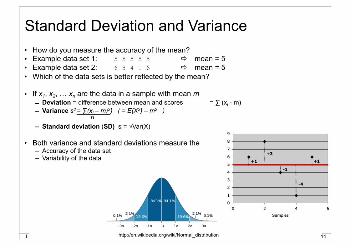
Standard Deviation and Variance• How do you measure the accuracy of the mean?• Example data set 1: 5 5 5 5 5 mean = 5• Example data set 2: 6 8 4 1 6 mean = 5• Which of the data sets is better reflected by the mean?

• If x1, x2, … xn are the data in a sample with mean m – Deviation = difference between mean and scores = ∑ (xi - m)– Variance s2 = ∑(xi – m)2) ( = E(X2) – m2 )

– Standard deviation (SD) s = √Var(X)

• Both variance and standard deviations measure the– Accuracy of the data set– Variability of the data

http://en.wikipedia.org/wiki/Normal_distribution 14

n


• Quantile– ‘Cut points' that divide a sample of data into groups containing (as far as possible) equal numbers of

observations.

• Quartile (Quantile of 4)– Values that divide a sample of data into 4 groups containing (as far as possible) equal numbers of

observations

• Percentile (Quantile of 100)– Values that divide a sample of data into 100 groups containing (as far as possible) equal numbers

of observations

Quantile, Quartile and Percentile

medianlower quartile upper quartile

15


Boxplots• Also known as

– box-and-whisker diagram– candlestick chart

• Quick overview of the most important values

Source: http://www.physics.csbsju.edu/stats/box2.html

16


Outliers• Try to avoid outliers!

– Improve your test equipment– Eliminate sources of disturbances– Repeat parts of your experiment in case

of disturbance

• Outliers are not generally bad – they give valuable information

• With large data sets outliers can often not be avoided

17


Creating Boxplots with Excel• Useful functions in Excel (and many other applications)

– MIN, MAX– MEDIAN– AVERAGE– QUARTILE– PERCENTILE

• Box Plots with Excel 2007– http://blog.immeria.net/2007/01/box-plot-and-whisker-plots-in-excel.html– http://www.bloggpro.com/box-plot-for-excel-2007/

18


Comparing Values• Significant differences between measurements?

value

frequency

mean A mean B

value

frequency

mean A mean B

19


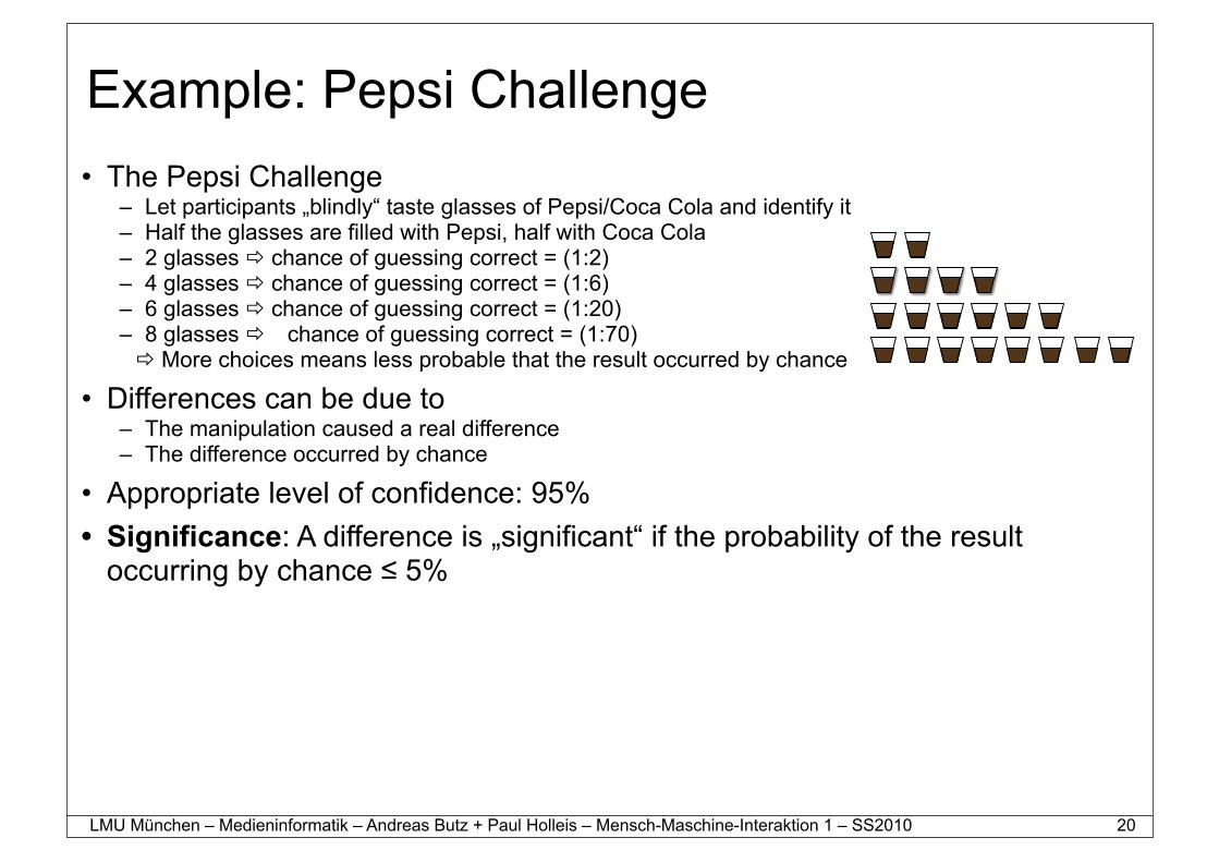
Example: Pepsi Challenge• The Pepsi Challenge

– Let participants „blindly“ taste glasses of Pepsi/Coca Cola and identify it– Half the glasses are filled with Pepsi, half with Coca Cola– 2 glasses chance of guessing correct = (1:2)– 4 glasses chance of guessing correct = (1:6)– 6 glasses chance of guessing correct = (1:20)– 8 glasses chance of guessing correct = (1:70) More choices means less probable that the result occurred by chance

• Differences can be due to– The manipulation caused a real difference– The difference occurred by chance

• Appropriate level of confidence: 95%• Significance: A difference is „significant“ if the probability of the result

occurring by chance ≤ 5%

20


Significance• In statistics, a result is called significant if it is unlikely

(probability p ≤ 5%) to have occurred by chance. • Never use the word significant if you don‘t mean

statistically significant!• It does not necessarily mean that the result is of practical

significance!

• T-Test can be used to calculate the probability p– The t-test gives the probability that both populations have the same mean (and thus their

differences are due to random noise)

• A result of 0.05 from a t-test is a 5% chance for the same mean

21


T-Test in Excel• Mean and T-Test can be calculated using MS Excel

– AVERAGE– TTEST

• TTEST(…) Parameters:1. Data row 12. Data row 23. Ends / Tails (e.g. A higher B => 1-tailed; A different from B => 2-tailed)4. Type (use ‘paired’ for within-subjects tests)

22


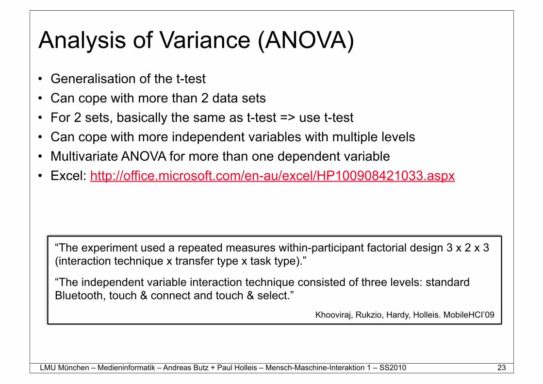
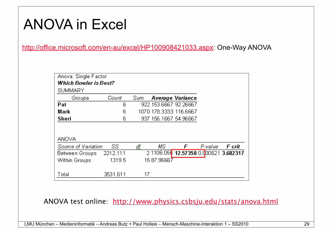
Analysis of Variance (ANOVA)• Generalisation of the t-test• Can cope with more than 2 data sets• For 2 sets, basically the same as t-test => use t-test• Can cope with more independent variables with multiple levels• Multivariate ANOVA for more than one dependent variable• Excel: http://office.microsoft.com/en-au/excel/HP100908421033.aspx

“The experiment used a repeated measures within-participant factorial design 3 x 2 x 3 (interaction technique x transfer type x task type).”

“The independent variable interaction technique consisted of three levels: standard Bluetooth, touch & connect and touch & select.”

Khooviraj, Rukzio, Hardy, Holleis. MobileHCI’09

23


For Researchers / the Geeks ...

24


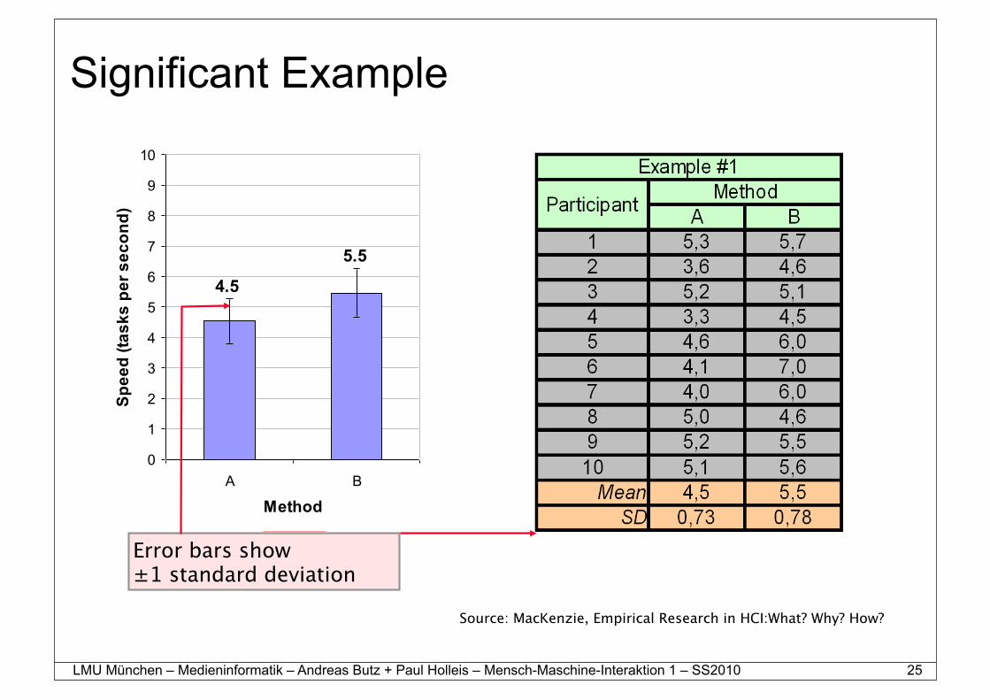
Significant Example

Error bars show±1 standard deviation

Source: MacKenzie, Empirical Research in HCI:What? Why? How?

25


Significant Example - Anova

Probability that the difference in the means is due to chance

Reported as…

F1,9 = 8.443, p < .05

Thresholds for “p”• .05• .01• .005• .001• .0005• .0001


26


Not Significant Example


Error bars show±1 standard deviation

27


Not Significant Example - Anova

Reported as…

F1,9 = 0.634, ns

Probability that the difference in the means is due to chance

Note: For non- significant effects, use “ns” if

F < 1.0, or p > .05 (if F > 1.0)


28


ANOVA in Excelhttp://office.microsoft.com/en-au/excel/HP100908421033.aspx: One-Way ANOVA

ANOVA test online: http://www.physics.csbsju.edu/stats/anova.html

29


Overview Parametric and Non-Parametric Experiment Design Parametric Test Non-Parametric Test

2 groups with different participants(one indep. variable)

Independent T-Test Mann-Whitney Test

2 groups with same participants (one indep. variable)

Dependent T-Test Wilcoxon Signed-Rank Test

≥ 3 levels groupswith different participantsand one indep. variable

One-way independent ANOVA

Kruskal-Wallis Test

≥ 3 levels groupswith same participantsand one indep. variable

One-way repeated measures ANOVA

Friedman‘s ANOVA

... ... ...

30


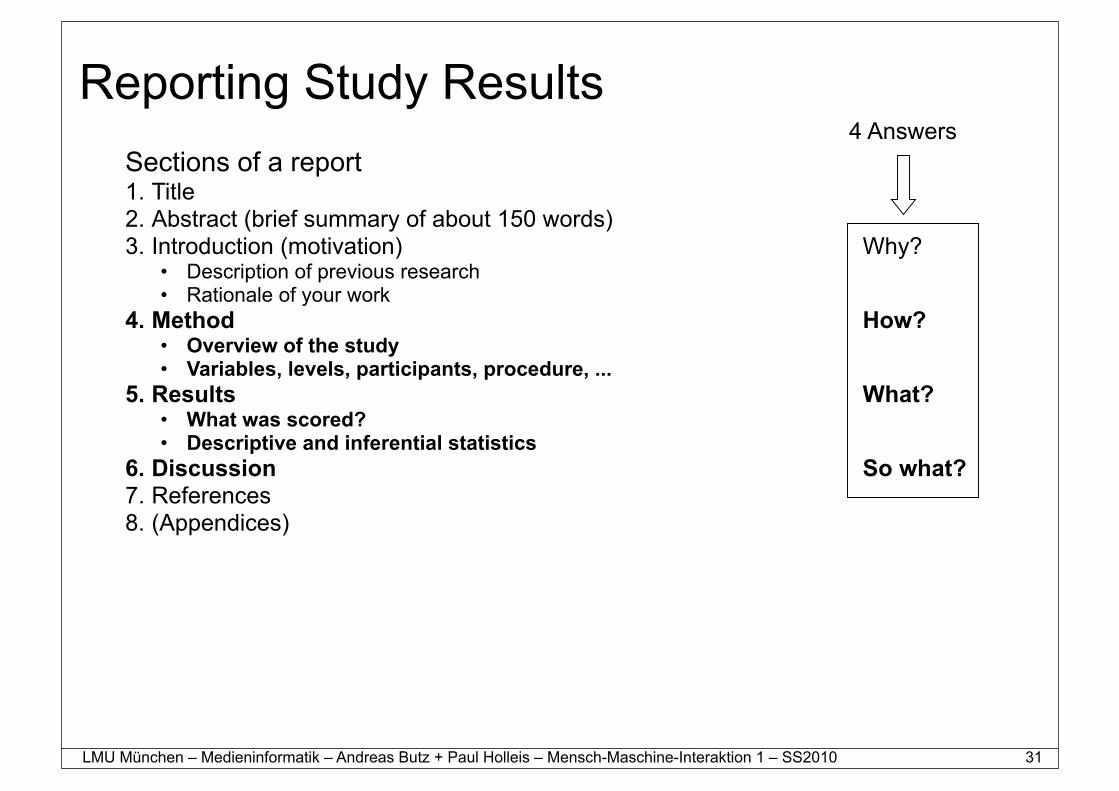
Reporting Study ResultsSections of a report 1. Title2. Abstract (brief summary of about 150 words)3. Introduction (motivation) Why?

• Description of previous research• Rationale of your work

4. Method How?• Overview of the study• Variables, levels, participants, procedure, ...

5. Results What?• What was scored?• Descriptive and inferential statistics

6. Discussion So what?7. References8. (Appendices)

31

4 Answers


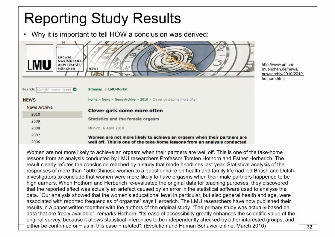
Reporting Study Results• Why it is important to tell HOW a conclusion was derived:

32

Women are not more likely to achieve an orgasm when their partners are well off. This is one of the take-home lessons from an analysis conducted by LMU researchers Professor Torsten Hothorn and Esther Herberich. The result clearly refutes the conclusion reached by a study that made headlines last year. Statistical analysis of the responses of more than 1500 Chinese women to a questionnaire on health and family life had led British and Dutch investigators to conclude that women were more likely to have orgasms when their male partners happened to be high earners. When Hothorn and Herberich re-evaluated the original data for teaching purposes, they discovered that the reported effect was actually an artefact caused by an error in the statistical software used to analyse the data. “Our analysis showed that the women's educational level in particular, but also general health and age, were associated with reported frequencies of orgasms” says Herberich. The LMU researchers have now published their results in a paper written together with the authors of the original study. “The primary study was actually based on data that are freely available”, remarks Hothorn. “Its ease of accessibility greatly enhances the scientific value of the original survey, because it allows statistical inferences to be independently checked by other interested groups, and either be confirmed or − as in this case − refuted”. (Evolution and Human Behavior online, March 2010)

http://www.en.uni-muenchen.de/news/newsarchiv/2010/2010-hothorn.html


This Lecture is not Enough!• We strongly recommend to teach yourself.

There is plenty of material on the WWW.

• Further Literature:– Andy Field & Graham Hole: How to design and report experiments, Sage– Jürgen Bortz: Statistik für Sozialwissenschaftler, Springer– Christel Weiß: Basiswissen Medizinische Statistik, Springer– Lothar Sachs, Jürgen Hedderich: Angewandte Statistik, Springer– Various books by Edward R. Tufte– ... and many more ...

33


References• Carmines, E. and Zeller, R. (1979). Reliability and Validity Assessment. Newbury Park:

Sage Publications• Colosi, L (1997) The Layman's Guide to Social Research Methods http://

www.socialresearchmethods.net/tutorial/Colosi/lcolosi1.htm • Field, A. and Hole, G. (2003). How to Design and Report Experiments. Sage Publications

34

Date post:	20-Nov-2021
Category:	Documents
Upload:	others
View:	2 times
Download:	0 times

Mensch-Maschine-Interaktion 1

Documents