HEDG Working Paper 10/21

Mental health, work incapacity and State transfers: an analysis of the British

Household Panel Survey

William Whittaker Matthew Sutton

August 2010

york.ac.uk/res/herc/hedgwp

Mental health, work incapacity and State transfers: an analysis of the British Household Panel Survey William Whittaker*, Matthew Sutton University of Manchester *Corresponding author: Abstract The UK has experienced substantial increases in the number of individuals claiming work incapacity benefit (IB) and the proportion of people claiming IB for mental health reasons. Following high-profile reports claiming that intervention would cost the State nothing, the Government has increased the availability of psychological therapies. The cost-neutrality claim relied on two statistics: the proportion of IB claimants diagnosed with mental and behavioural disorders; and estimates of the costs to the State of periods on IB. These are cross-sectional associations. We subject these two associations to more rigorous longitudinal analysis using nationally representative data from seventeen waves (1991-2007) of the British Household Panel Survey (BHPS). We model the effect of depression on (a) State transfers and (b) the probability of being on IB whilst controlling for covariates and unobservable heterogeneity. Our results reveal that cross-sectional associations with depression are substantially confounded. The estimated effects of becoming depressed on State transfers reduce by 83% and 88%, and on the probability of claiming IB drop to just 0.4 and 0.7 percentage points, for males and females respectively. We conclude that the stated benefits of reducing depression for the State and for labour market participation have been substantially over-estimated. Key words: Work incapacity, Mental health, Dynamic modelling, Unobserved heterogeneity JEL Classification: C23, H51, I10, I18 Contact: William Whittaker

Health Sciences - Health Economics University of Manchester 4.304, Jean McFarlane Building, Oxford Road, Manchester M13 9PL United Kingdom Telephone: +44(0)161 306 8002 Fax: +44(0)161 275 5205 E-mail: william.whittaker@manchester.ac.uk

Acknowledgements: The British Household Panel Survey was made available through the ESRC Data Archive. The data were originally collected by the ESRC Research Centre on Micro-social Change at the University of Essex (now incorporated within the Institute for Social and Economic Research). Neither the original collectors of the data nor the Archive bear any responsibility for the analyses or interpretations presented here. The authors thank both organisations for providing access to the data. The comments of participants at the January 2009 Health Economists’ Study Group (in particular, Nicholas Ziebarth) and the 2009 British Household Panel Survey Conference are gratefully acknowledged. Conflict of interest: Neither authors have any conflict of interest relating to this research, nor are there any political conflicts of interests related to this work.

2

1. INTRODUCTION

Individuals in the UK who have been unable to work for over 28 weeks because of ill-health

are entitled to claim Incapacity Benefit (IB) from the State. The number of people claiming IB

has increased by over 300% in 30 years (McVicar and Anyadike-Danes, 2008) and now

represents approximately 6.5% of the working-age population. During a period of apparent

stability in work incapacity claiming rates over the past decade, the proportion of claimants

claiming for reasons of mental health rose from 32% to 45%.

In 2007 the Government committed itself to reducing the number of people claiming IB by 1

million. This target is part of a wider aim by the Government to reach an 80% employment

rate by 2016 (Freud, 2007). Mental health and IB claiming have become a growing concern,

and something the Government seem dedicated to reduce. In the 2007 Comprehensive

Spending Review (H.M Treasury, 2007) the Government committed itself to improving

access to psychological therapies for those with depression or anxiety as a Public Service

Agreement (PSA) target. The NHS programme, Improving Access to Psychological Therapies

(IAPT) [http://www.iapt.nhs.uk/], is the process by which this PSA target will be delivered.

Cognitive Behavioural Therapy (CBT) forms a large component of the IAPT programme and

has been recommended by the National Institute for Health and Clinical Excellence (NICE) as

an effective treatment for depression in 2004 (NICE, 2004 (amended 2007, updated 2009)).

Two IAPT pilot schemes were put into place in 2007/2008. By spring 2010 112 of the 152

Primary Care Trusts were offering some form of CBT (DH, 2008, 2010). By 2010/2011 the

objectives are to have: access to some form of CBT in each area (DH, 2010); 900,000 people

3

treated; 3,600 newly trained therapists; and 25,000 fewer sickness benefit claimants (NHS,

2010). Investment for the programme in 2010/2011 is in excess of £173 million.

The high-level commitment to this programme followed influential reports by the Centre for

Economic Performance’s Mental Health Policy Group at the London School of Economics. In

2006 Layard made the case for expanding the availability of psychological therapies in the

British Medical Journal (Layard, 2006). This was supported by a more substantial report

(Layard et al., 2006a) and a number of other papers published on the LSE Programme website

[http://cep.lse.ac.uk/research/mentalhealth/] including a draft cost-benefit analysis (Layard et

al., 2006b).

The case described in the cost-benefit analysis relies on two key statistics: (i) that the

proportion of IB claimants diagnosed with mental and behavioural disorders is 40%; and (ii)

that the treatment will result in higher contributions to the State Exchequer. The second of

these statistics was calculated using predicted tax gains earned in employment minus the

benefits previously paid to people with depression on IB. Based on a (one-off) £750 cost per

treatment cycle, Layard et al. (2006b) estimated that the treatment would pay for itself within

a year. Overall, these findings led Layard et al. (2006b) to suggest that increasing the

availability of psychological therapies “would cost the Exchequer nothing” (p.1; emphasis

in original).

Both findings are cross-sectional associations but are used to predict the effects of changes in

the level of depression. In this paper we subject these two simple empirical findings to a more

rigorous longitudinal analysis. We first estimate the effect of depression on contributions to

4

the Exchequer. We then examine whether becoming depressed affects the probability of

claiming IB.

Our first analysis addresses more comprehensively how depression influences the

contribution that individuals make to the Exchequer. We use longitudinal data and capture

information on contributions made via income tax and National Insurance on earnings and

claims made on a wide range of state benefits including IB. To our knowledge this is the first

study to model Exchequer contributions using longitudinal data, and the first to model the

financial impacts of health conditions on individual contributions to State finances.

Our second analysis assesses the relationship between depression and work incapacity. While

there is a wide literature on IB claiming, little has been done that exploits individual-level

longitudinal data to model the dynamics of IB claiming. Most studies have been cross-

sectional (Disney and Webb, 1991; Nolan and Fitzroy, 2003; McVicar, 2006) or have used

aggregate data (typically the DHSS, Molho, 1989, 1991; Holmes and Lynch, 1990; Lynch,

1991). This paper uses longitudinal data that enables us to model changes in IB claiming

status as a function of changes in mental health status and a wide range of other covariates.

Another limitation of past studies has been the lack of detailed data on health conditions.

Molho (1989, 1991) proxied for health with the claiming of sickness benefits in a study using

DHSS data. Disney and Webb (1991) used smoking status as the health measure in a study

using the Family Expenditure Survey. Faggio and Nickell (2005) and McVicar and Anyadike-

Danes (2008) both used self-reported disability. Two studies have examined the main health

reason for claiming IB. Holmes and Lynch (1990) and Lynch (1991) found that the main

health reason for claiming IB had a significant effect on off-flows in the 1980s.

5

Previous studies have not therefore explicitly controlled for any potential confounding of the

effects of other health problems. The British Household Panel Survey (BHPS) data we use in

this study enables us to control for several health conditions, including problems with arms

and legs, sight, hearing, skin, chest, heart and blood, stomach, diabetes, epilepsy, and

migraines.

2. DATA

We use the BHPS to model IB, depression, and contributions to the Exchequer for the period

1991-2007. The BHPS was designed as an annual survey of each adult (16+) member of a

nationally representative sample of more than 5,000 households. The same individuals are re-

interviewed in successive waves and, if they split-off from original households, all adult

members of their new households are also interviewed. Children are interviewed once they

reach the age of 16. Thus the sample should remain broadly representative of the population

of Britain as it changes through time (Taylor et al., 2010).

A number of booster samples have been added to the BHPS (Taylor et al., 2010). In 1997

(Wave 7) a sub-sample of the original United Kingdom European Community Household

Panel (UKECHP), comprising all households in Northern Ireland who were still responding to

the UKECHP and a low-income sample of the Great Britain panel, was introduced. Funding

for this sub-sample ended in 2001 (Wave 11). In 1999 (Wave 9) booster samples of 2,399

individuals in Scotland and 2,191 individuals in Wales were introduced. In 2001 (Wave 11)

6

the Northern Ireland Household Panel Survey added 1,979 households and 3,528 individuals

(+ 200 proxy interviews) to the BHPS.

IB is measured using the variable f125, which asks respondents: ‘Have you yourself (or

jointly with others) since 1st September last year received Incapacity Benefit?’ There are

several important points to note here. First, this measure is retrospective. Second, the timing

of interviews in the BHPS varies and as such the period covered by the question varies across

observations. Third, this measure does not provide information on the number or duration of

claim spells.

We are interested in the relationship between mental health and work incapacity, and as such,

we restrict our sample to those of working age. As the IB claiming question is retrospective,

we include women aged 17-61 years, and men aged 17-66 years at the time of the interview.

Depression is measured using the variable hlprbi, which asks respondents: ‘Do you have any

of the health problems or disabilities listed on this card…’. One of the listed conditions is

‘Anxiety, depression or bad nerves’. An alternative measure of mental health included in the

BHPS is the 12 question version of the General Health Questionnaire (GHQ-12) (Goldberg et

al., 1997). We replicate our analysis with the ‘caseness’ definition of this variable, with

individuals reporting a score of 4 or more defined as having mental ill-health.

To measure Exchequer contributions, we use data from the income section of the BHPS.

Payments to the Exchequer are measured using income tax paid, which is calculated as the

difference between gross and net usual monthly pay (variables paygty and paynty,

respectively). To measure payments from the Exchequer, we use the variable fimnb, which

7

measures the amount of benefit income an individual received in the last month (jointly

received benefits are apportioned equally unless otherwise stated). This contribution measure

does not represent total individual payments to the Exchequer as we only have data on

employment taxes/National Insurance payments. Income tax and National Insurance

accounted for approximately 52% of Public Sector receipts and social benefits accounted for

approximately 35% of Public Sector expenditure over the period 1992-2002 (ONS, 2010a).

We deflate contributions by the annual Retail Price Index obtained from the Office of

National Statistics (ONS, 2010b).

We measure socio-economic group differences using the Registrar General’s Social Class.

The manual social class comprises skilled, partly-skilled and unskilled manual workers and

the armed forces. Where the individual is unemployed then their last occupation is recorded.

If there is no information on the individual’s employment (because they have never worked,

say) then we take the head of the household’s occupation status, father’s status, and mother’s

status in respective order.

The strength of the local labour market may also have an impact on the probability of

claiming IB. Job destruction, where people find themselves out of work, can be measured by

the unemployment rate for the area. A high unemployment rate may encourage higher IB

claiming rates, and those with health problems may be more likely to transit onto IB once

becoming unemployed. This can be described in two ways (Beatty et al., 2000): (i) the

redundancy effect, whereby people of poorer health are more likely to be made redundant,

and (ii) the benefit shift, whereby people of poorer health are seen as relatively unattractive to

employers compared to the healthy unemployed and are persistently sent to the back of the

job queue as new waves of people enter unemployment. In both cases, those in poorer health

8

switch to IB as it pays higher than unemployment benefit. To capture variations in the

strength of the local labour market, we utilise Local Authority District (LAD) level data on

unemployment rates and average wage rates. This information was obtained from the

claimant count (ONS, 2010c), and the Annual Survey of Hours and Earnings (ASHE, 2010),

via NOMISWEB (NOMISWEB, 2010). LAD identifiers for the BHPS were provided by

Data-Archive (BHPS, 2009). Average wage rates are included to proxy the replacement rate

of IB rates to local wages – given IB rates are national rates, the average regional wage

captures regional differences in the relative generosity of IB payments.

3. METHODS

3.1 Effect of depression on Exchequer contributions

The first stage of our analysis is to test and quantify the effects of depression on contributions

to the Exchequer. An individual’s net contribution ( iC ) to the Exchequer at time t can be

estimated as:

ititit BTC −= (1)

in which itT is taxes paid and itB is state benefits received.

We use pooled OLS to estimate the following equation:

ititkkit vxC += β (2)

9

Where itC is monthly contribution per individual, and itkx is a range of k covariates that may

affect the amount of contributions made by individuals. These will include factors influencing

whether someone is in work (and thus pays taxes) and/or claiming benefits.

To ensure we have reliable estimates, we need to control for potential bias in the model. The

first possible source of bias occurs were there to be reverse causality between the dependent

variable (contributions) and one of our independent variables. Our primary interest is in the

effect of depression. Reverse causality would require depression to be caused by contributions

to the Exchequer - we believe this causal pathway is unlikely. The second potential source of

bias stems from unobserved heterogeneity; certain individuals may be more or less likely to

contribute than others and these unobservable differences may be correlated with other

independent variables. To correct for this potential source of bias, we estimate (2) using fixed-

effects assuming that the unobserved component is time invariant. Use of fixed-effects also

controls for any time-invariant, individual-specific measurement errors:

itiitkkit vuxC ++= β (3)

3.2 Effect of depression on IB Claiming

There are two important methodological concerns with modelling IB claiming and depression.

First, there are likely to be unobservable individual characteristics that influence whether

someone claims IB, including attitudes to health and/or the State. For example, older people

are more reluctant to claim off the State (Costigan et al, 1999; Kotecha et al., 1999), which

would exert negative bias on the estimated age gradient. These unobserved characteristics are

likely to be correlated with the variables in our model. Second, IB claiming is likely to be

10

persistent as claims for ill health may persist for a number of years for those with long-term

health conditions. It is important to remove any correlation between the dependent variable

and the error term for our estimates to be unbiased.

We follow Wooldridge (2005) in estimating a dynamic probit model with unobserved effects:

itiititit ucyzy ++++= −1310 βββ (4)

Here ity is a binary indicator for claiming IB at some point in the next year, 1−ity is a binary

indicator for whether the individual claimed IB in the last year, and ic is an individual

specific time-invariant error term that we allow to be correlated with itz , a vector of

covariates. itz contains dummy variables for other health problems and a range of variables

found to be significant predictors for IB claiming in the literature: age, region of residence,

education, ethnic group, marital status, number of children, socioeconomic group, area wage

and unemployment rates, and wave/year.

itz also contains an indicator for the recall period for the individual. This is the difference in

days between the start of the recall period (1st September of the previous year) and the

interview date. This controls for the possibility that individuals with longer recall periods

have a longer period at which to have been at risk of claiming IB.

We relax the (strong) assumption of zero heterogeneity in three ways, we include an initial

condition, 0iy which is a binary variable indicating whether individual i reported having

claimed IB in their first observation, time averages of the covariates, iz , and individual

random-effects, ia :

11

( )220100 ,~,| aiiiii zyNormalzyc σααα ++ (5)

with iiii azyc +++= 2010 ααα where ( )20 ,0~),(| aiii Normalzya σ .

The first additional term, 0iy ; is included in recognition that our sample is left-truncated,

meaning we have little/no information on an individuals’ IB claiming history before they

enter the survey. 0iy is included since the first observation may hold some indication for any

unobserved tendency for an individual to claim IB. Our second additional term are iz , here

we assume that any heterogeneity among individuals that is correlated with the covariates in

the model works only through the time averages of the (time varying) covariates in itz , iz ,

thus removing any correlation between the heterogeneity term and itz . The third additional

term, ia , assumes a time-invariant individual-specific random-effects specification.

Substituting (5) into (4) gives:

itiitiitit uazyyzy ++++++= − 4130210 βββββ (6)

The difference between this dynamic random-effects model and a standard random-effects

probit model is the inclusion of additional terms 1−ity , 0iy and iz . It assumes that (i) having

conditioned on the covariates and unobserved heterogeneity: itz and ic , the dynamics are

correctly specified as first order, (ii) ic is additive in the standard normal cumulative

distribution function, and (iii) the itz are strictly exogenous.

12

Following the literature (Molho, 1989, 1991; Holmes and Lynch, 1990; Lynch, 1991;

McVicar and Anyadike-Danes, 2008) we estimate separate models for males and females.

The models are estimated using xtprobit, re in STATA v11.0.

4. RESULTS

4.1 Descriptive statistics

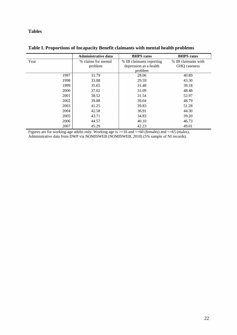
Table I compares the proportion of IB claimants claiming for mental health problems from

national administrative data, with the proportions of IB claimants in the BHPS reporting

problems with depression and GHQ caseness. While the proportion of IB claimants in the

BHPS reporting problems with depression (GHQ caseness) is lower (higher) than national

figures, both rates follow similar trends to the national trend.

[Table I. Here]

The initial sample of working age adults is 181,674 person-year observations (27,440

individuals). Use of one period lead values of IB claimant status reduces the sample to

156,513 observations (22,290 individuals). Item non-response on the remaining covariates

results in a final sample of 145,125 person-year observations, comprising 69,436 observations

for males and 75,689 observations for females (10,354 male individuals and 10,849 female

individuals). Our panel is unbalanced and individuals can enter or leave the sample at any

wave. When including aggregate LAD variables the sample is restricted to waves 8-17 (1998-

2007) and excludes Northern Ireland. This reduces the sample to 82,241 person-year

13

observations (39,446 male observations and 42,795 female observations) and 14,981

individuals (7,266 men, 7,715 women).

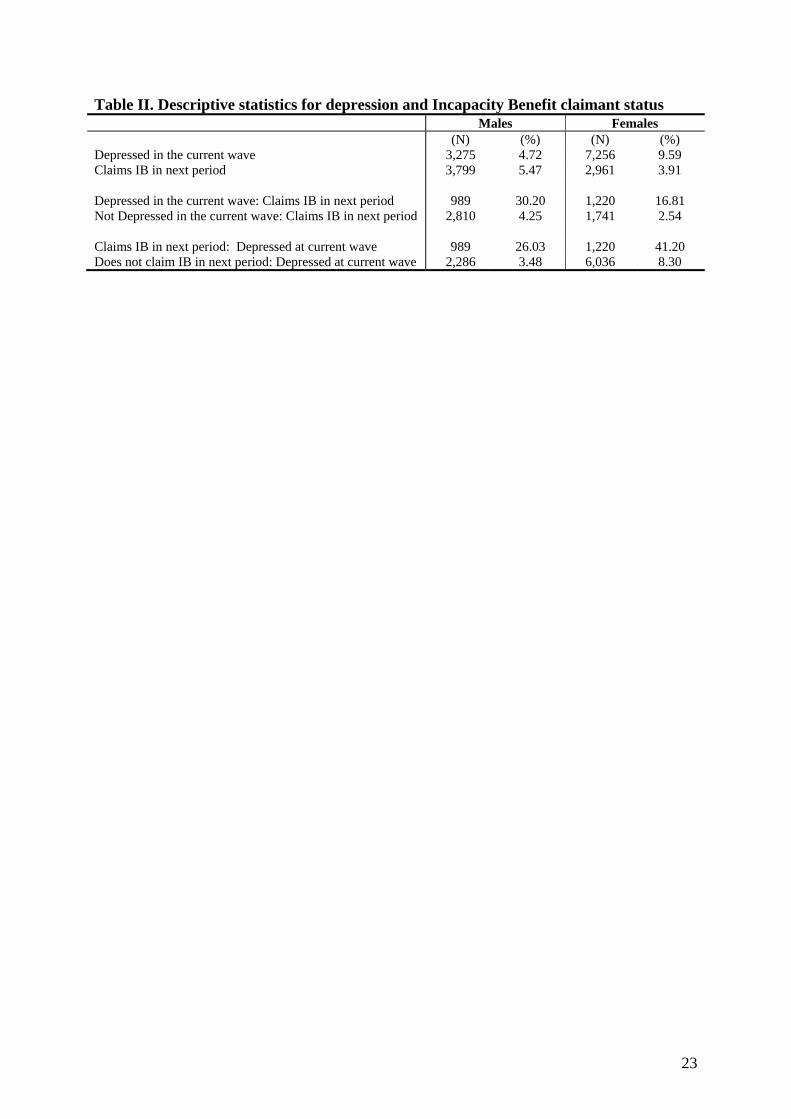
Table II provides summary statistics on rates of depression and IB claiming in the next period,.

For females there is a higher prevalence of depression than IB claiming. Higher rates of

illness than IB claiming is not unusual. Sly et al. (1999) report 3.2 million people were active

in the labour market though eligible for IB benefits in 1998/99 (for a discussion on these

‘hidden sick’ see Beatty et al., 2000).

[Table II. Here]

Approximately 26% of men and 41% of women who claim IB in the next period are

depressed. While depression is more prevalent for women, depression appears to have a

much stronger effect on claiming IB in the next period for males. Thirty percent of depressed

males claim IB in the next period compared with 4% of non-depressed males. The equivalent

figures are 17% and 3% for females.

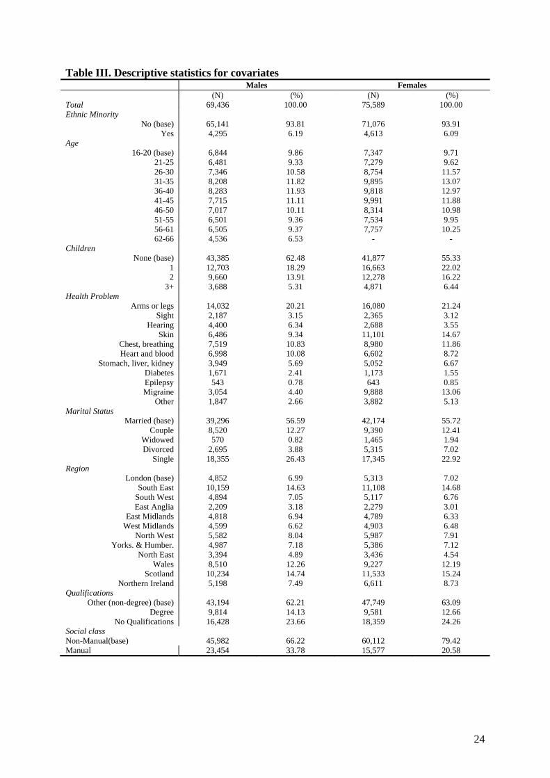
Table III provides average values of the covariates. There is a clear distinction between the

prevalence of health conditions amongst males and females. Skin, chest/breathing, migraines,

and stomach/liver/kidney problems are all of a higher prevalence in females than males.

Males have higher rates of problems related to hearing, heart/blood, and diabetes.

[Table III. Here]

14

4.2 The effect of depression on Exchequer contributions

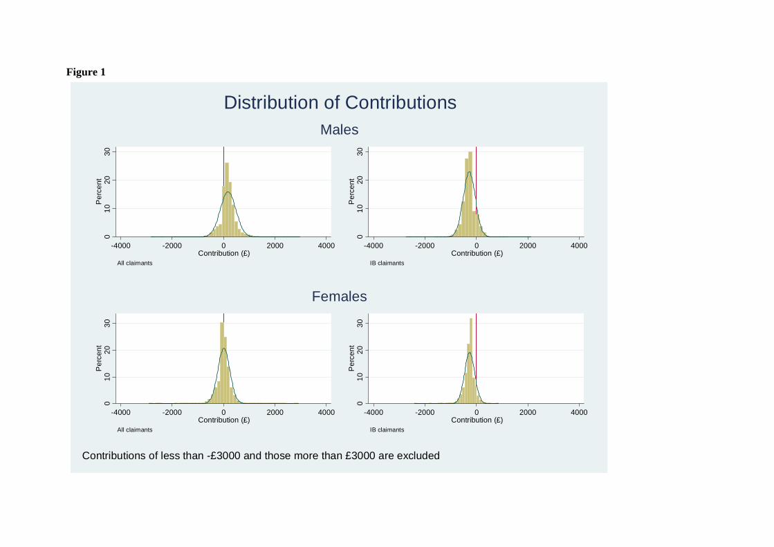
The distribution of the variable we have calculated is plotted in Figure 1. Our contribution

measure suggests males on average contribute more than females, and as expected, the

majority of IB claimants make a negative contribution to the Exchequer.

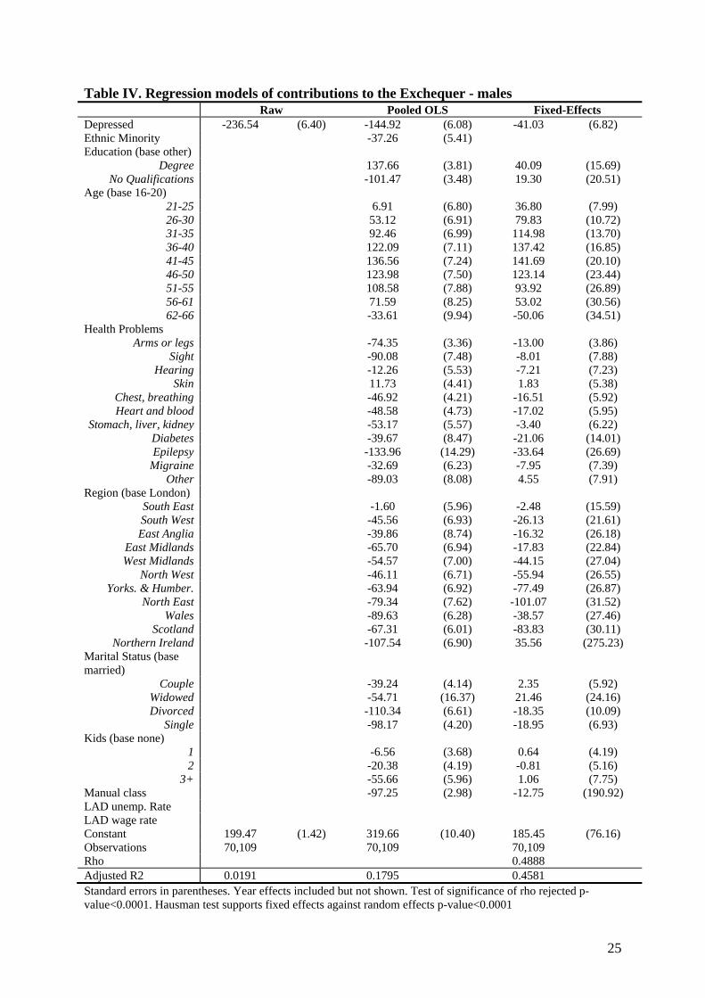
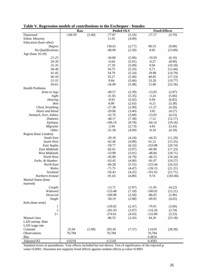
The results from estimating equation (3) with pooled OLS and fixed-effects models are given

in Tables IV and V. In the pooled model the estimated effects of depression on contributions

to the Exchequer are -£145 and -£78 for males and females respectively. In a model estimated

on the same sample that excludes the other covariates, these coefficients equal -£237 and -

£141. Thus, £92 (£63 for females) of the difference in the Exchequer contributions of the

depressed and non-depressed is attributable to (a limited range of) observable covariates. The

crude difference suffers substantially from omitted variable bias. In a model with only

depression and a dummy variable for IB claimant (not shown), the estimate for depression

falls from -£237 to -£109 for males (-£141 to -£102 for females). Thus IB claiming is only a

partial measure of the impact of depression on contributions to the Exchequer.

The results in the third columns of Tables IV and V control for unobserved heterogeneity.

Almost a half, (48.9% for males, 48.2% for females) of the unobserved variation in

contributions to the Exchequer is explained by the unobserved heterogeneity term. Tests of

the null that the unobserved effects are not significant are rejected (p-values <0.0001) and as

such we favour the third set of results obtained from fixed-effects estimation. This model

suggests that depression ‘costs’ the Exchequer £41 per month for depressed males (£17 per

month for depressed females). These effects are substantially smaller than the £145 and £78

in the pooled model which implies that individuals who report depression are more likely to

15

have unobservable characteristics that are associated with smaller contributions to the

Exchequer.

Our other estimates work in the direction expected. An increased presence of children reduces

net State contributions, education increases contributions, and there is a clear business cycle

effect (not reported) for males with greater contributions when the economy was growing

(negative contributions during the 1992 recession, with contributions increasing from 1994 in

the fixed-effects specification). For females we find contributions decrease over the sample

period.

[Table IV. Here]

[Table V. Here]

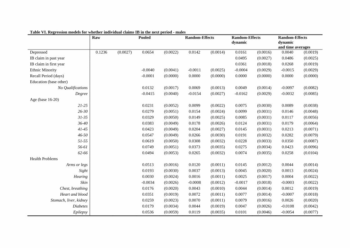
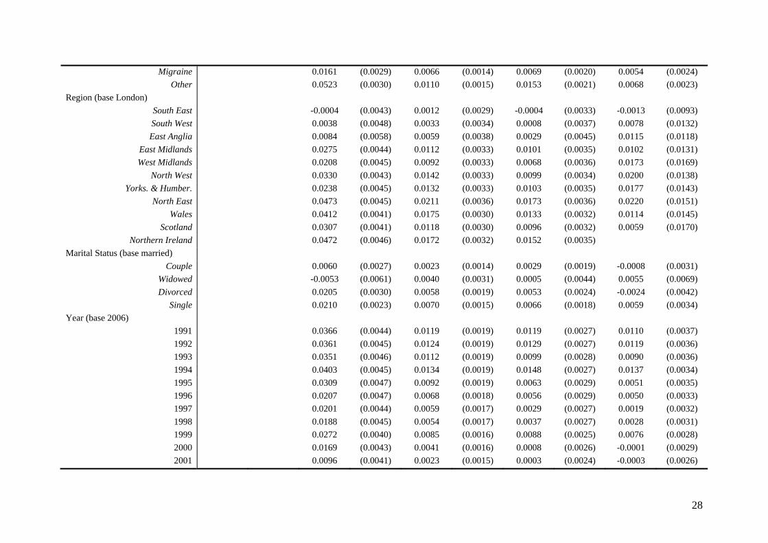
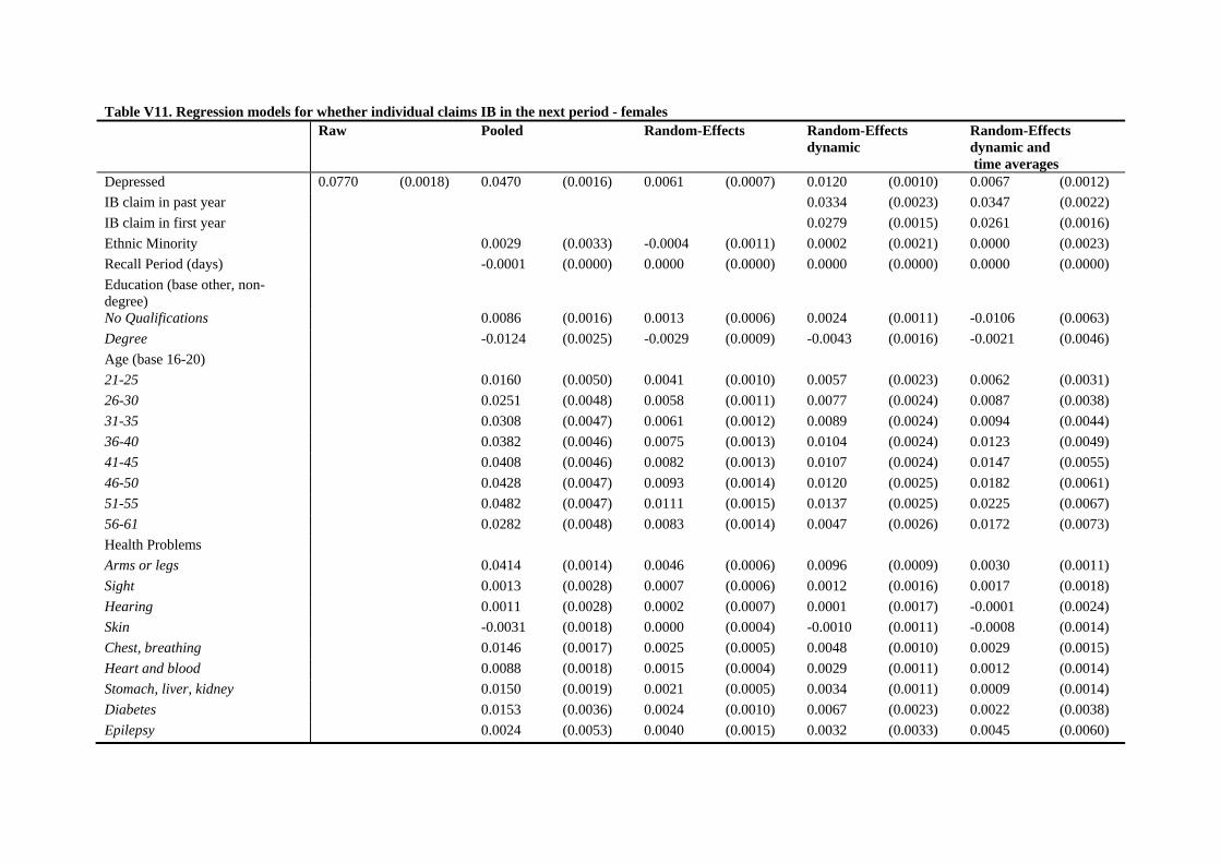
4.3 The effect of depression on IB claiming

The results from multivariate analyses are provided in Tables VI and VII for males and

females respectively. The estimates are reported as average marginal effects. In the first

column of results being depressed increases the probability of claiming IB in the next wave

by 12.4% for males and 7.7% for females. The results in the pooled model suggest a lower but

still strongly significant positive effect of reporting depression on the probability of claiming

IB in the next wave.

The third sets of results are from the static random-effects specification. The estimated effect

of depression is significantly reduced to 1.4% for males (0.6% for females) and suggests there

are positive correlations between the unobserved effects and depression. The fourth set of

16

results is from the dynamic random-effects specification, which includes the lagged value of

IB claimant status and the initial observed IB status. Both terms are highly significant for both

genders and imply persistence in IB claiming.

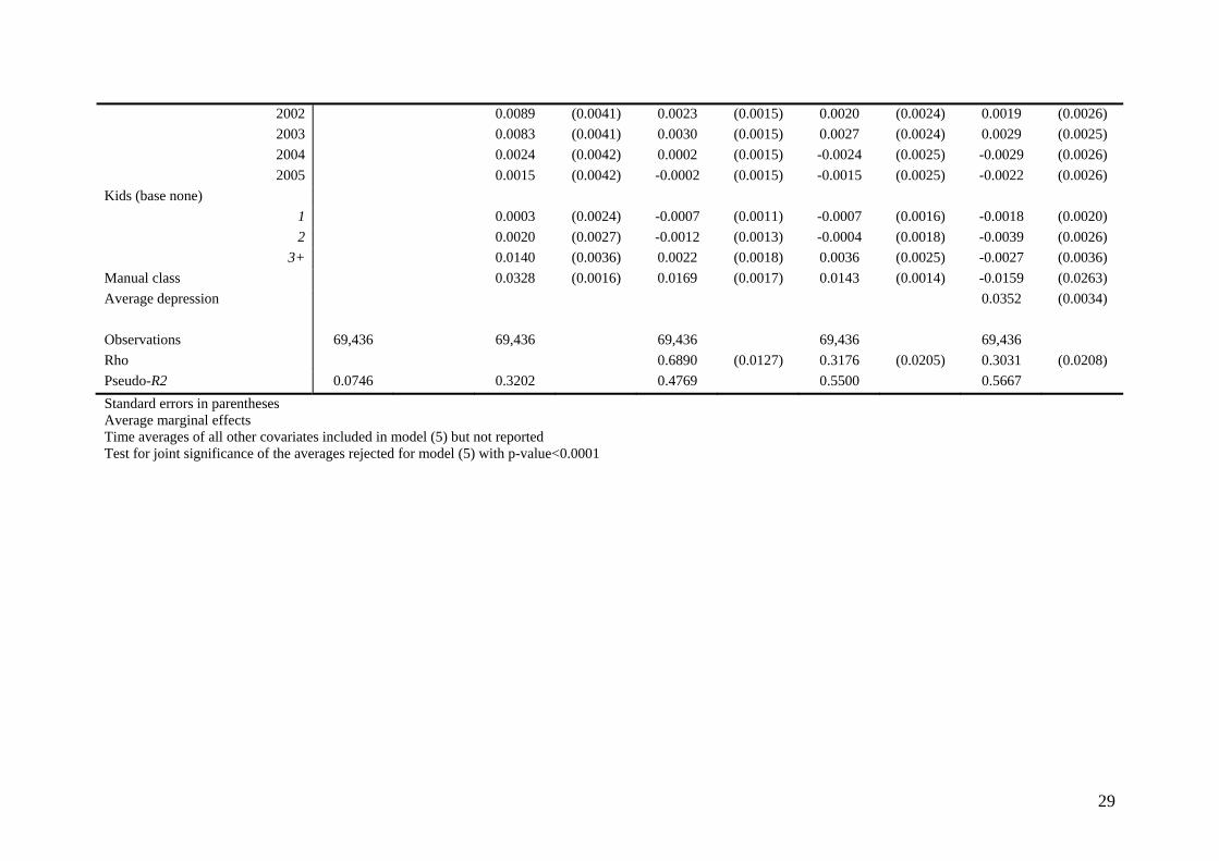
The fifth set of results are from the full dynamic model including the averages of the time-

varying variables (equation (6)). These average values are jointly significant for both sexes.

The estimated effect of depression is now reduced from 12.4% to 0.4% for males, and from

7.7% to 0.7% for females. The estimated coefficients on the average depression variable are

positive and significant for both genders. Since this controls for any correlation of the

unobserved heterogeneity with the time average of depression, we are unable to disentangle

the effect of long(er) term depression from unobserved heterogeneity. Controlling for

individual specific and time invariant heterogeneity drives the coefficients on the regional,

manual, and marital status dummies to insignificance because there is little within-respondent

variation in these variables.

[Table VI. Here]

[Table VII. Here]

Table VIII contains the key results from the models estimated over the shorter period (1998-

2007) including area wage and unemployment rates. The first panel contains the results from

the final models of Tables VI and VII. The second panel of results are where the area rates are

included. For comparability, the third panel of results are for models estimated on the smaller

sample excluding the area rates. The effect of depression is reduced further to an insignificant

0.1% for males, but the second panel of results reveal that this decline is due to the change in

the sample. For females the effect of depression is constant across all three models at 0.7%.

17

While we find no evidence of a significant effect of local wages, we do find a positive effect

of unemployment for males and females.

[Table VIII. Here]

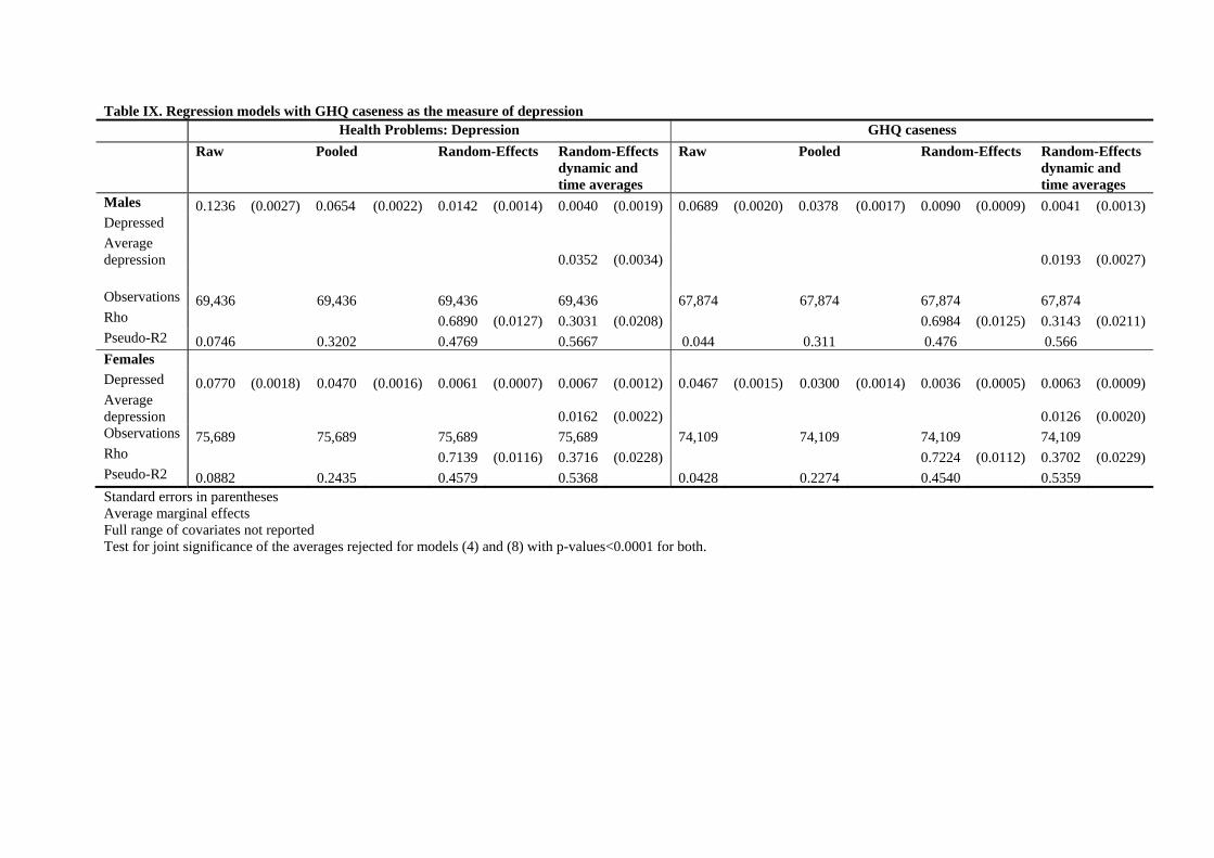
Our interest lies in the effect of depression on the probability of IB claiming in the following

year. Table IX gives the key results where we model depression using a binary variable for

GHQ caseness. The estimates are essentially the same across the range of models, though we

find a slightly smaller impact of GHQ caseness on the probability of claiming IB.

[Table IX. Here]

5. DISCUSSION

In our first analysis, we find depressed males and females have statistically significant

reduced contributions to the Exchequer, though this is much smaller once we control for

several confounding factors. In our second analysis, we find a positive association between

depression and IB claiming but this effect is reduced, though remains significant and positive,

when we control for a number of other factors that influence IB claiming.

Making the model dynamic effectively permits past depression to affect the probability of

claiming IB. The total effect of depression thus comprises of an immediate effect, or short-run

elasticity; given by the estimated coefficient for depression; an average effect, and a long-run

elasticity which is the product of recursive effects of past depression. Given the estimates for

18

lagged IB claiming for males and females in our preferred specifications are small (0.0486

and 0.0347), the long-run elasticity is likely to be small – for example, a one period lagged

impact of depression would be 0.00019 (=0.0486*0.0040) for males and 0.00023

(=0.0347*0.0067) for females.

One way of interpreting the current depression and average-depression estimates is in a

temporal setting. The current depression indicator measures the impact of changes in

depression, while the average-depression measure picks up a longer-term propensity to

depression. Hauck and Rice (2004) find significant mobility in mental health in the BHPS

using the GHQ score suggesting there is enough variation to distinguish between these effects.

Comparing across the health conditions, we find that depression has the largest impact on

Exchequer conditions with the exception of epilepsy for females. Depression also had the

highest effect on the probability of claiming IB over all other conditions listed for females.

For males, however, the effects of arms and leg problems, diabetes, migraine, and other

conditions were larger. There are large and significant effects of these other health problems

in most models. This suggests that there would be significant confounding were we to exclude

these other problems.

We find an increasing probability of claiming IB by age group for both genders. Similar age

effects have been found in Molho (1989, 1991) for on-flows, Lynch (1991) and Holmes and

Lynch (1990) for reduced off-flows, and Disney and Webb (1991) for IB claiming.

We find no significant effect of area wage rates for either gender, which contrasts with

positive effects for on-flows to IB for income and rate of benefit found in Molho (1989) and

19

negative effects of IB rates on off-flows in Holmes and Lynch (1990) and positive effects of

replacement rates on IB claiming in Disney and Webb (1991). However, our results show a

significant effect of higher unemployment rates on the probability of claiming IB for males.

Positive effects of local unemployment rates have been found by Beatty et al (2000) and

Disney and Webb (1991), and negative effects for off-flows (Lynch, 1991; Holmes and Lynch,

1990). Insignificant unemployment rates were found in studies for IB on-flows by Molho

(1989, 1991).

There are a number of limitations to our analyses. Our measure of contributions to the

Exchequer contains only financial transactions, but this is not the only means by which

individuals contribute to the Exchequer. Transfers can occur via taxes on spending and there

are substantial transfers in the form of state-financed health care provision. While the BHPS

does contain some measures of health care utilisation, they are insufficiently detailed to

incorporate into the transfers measure. Attrition is likely to be higher amongst individuals

with poor health – this has been confirmed in Contoyannis, Jones and Rice (2004) who use

the BHPS to analyse health dynamics. This could lead to negative bias on the effect of

depression if those attriting were also more likely to claim IB. Attrition however, was found

to have an insignificant impact on the estimated determinants of self-reported health in

Contoyannis, Jones and Rice (2004).

Nevertheless, our results suggest that univariate cross-sectional associations between

depression and work incapacity and State transfers are substantially inaccurate estimates of

the causal effects. The estimated effects of becoming depressed on State contributions reduce

by 83% and 88%, and on the probability of claiming IB drop to just 0.4 and 0.7 percentage

points, for males and females, respectively.

20

References

Anyadike-Danes M. 2009. What is the problem, exactly? The distribution of Incapacity Benefit claimants’ conditions across British regions. ERINI Monographs: ASHE. 2010. The Annual Survey of Hours and Earnings 1997-2007. Office for National Statistics. Beatty C, Fothergill S and MacMillan R. 2000. A theory of employment, unemployment and sickness. Regional Studies 34 : 617-630. British Household Panel Survey. 2009. Data files and associated documentation. The Data Archive and the ESRC Research Centre on Micro-social Change: Colchester. Contoyannis P, Jones A.M, Rice N. 2004a. Simulation-based inference in dynamic panel probit models: an application to health. Empirical Economics 29 : 49-77. Costigan P, Finch H, Jackson B, Legard R, Ritchie J. 1999. Overcoming Barriers: Older People and Income Support. Department of Social Security Research Report 100. Corporate Document Services: Leeds. Department of Health. 2008 Improving Access to Psychological Therapies – Implementation Plan: National guidelines for regional delivery. London: Department of Health. Department of Health. 2010. Realising the Benefits – IAPT at Full Roll Out. London: Department of Health. Disney R, Webb S. 1991. Why are there so many long term sick in Britain? The Economic Journal 101 : 252-262. ESA. 2010. http://www.direct.gov.uk/en/DisabledPeople/FinancialSupport/esa/index.htm [31 July 2010]. Department for Work and Pensions. Faggio G, Nickell S. 2005. Inactivity Among Prime Age Men in the UK. Discussion Paper No. 673. Centre for Economic Performance: London. Fothergill S. 2001. The true scale of the regional problem in the UK. Regional Studies 35 : 241-246. Freud D. 2007. Reducing Dependency, Increasing Opportunity: Options for the Future of Welfare to Work. London: Department for Work and Pensions. Goldberg D.P, Gater R, Sartorius N. et al. 1997. The validity of two versions of the GHQ in the WHO study of mental illness in general health care. Psychological Medicine 27 : 191–197. H.M. Treasury. 2007. Pre-Budget Report and Comprehensive Spending Review: PSA Delivery Agreement 18: Promote better health and wellbeing for all. Hauk K, Rice N. 2004. A longitudinal analysis of mental health mobility in Britain. Health Economics 13 : 981-1001. Holmes P, Lynch M. 1990. An analysis of Invalidity Benefit claim duration for new male claimants in 1977/1978 and 1982/1983. Journal of Health Economics 9 : 71–83. IB. 2010. http://www.direct.gov.uk/en/DisabledPeople/FinancialSupport/IncapacityBenefit/index.htm [31 July 2010]. Department for Work and Pensions. Kotecha M, Callanan M, Arthur S, Creegan C. 1999. Older people’s attitudes to automatic awards of Pension Credit. Department for Work and Pensions Research Report No 579. Layard R. 2006. The case for psychological treatment centres. British Medical Journal 332 : 1030-1032.

21

The Centre for Economic Performance’s Mental Health Policy Group (Chaired by Lord Layard). 2006a The Depression Report: A New Deal for Depression and Anxiety Disorders. London School of Economics. Layard R, Clark D, Knapp M, Mayraz G. 2006b. Implementing the NICE guidelines for depression and anxiety. A cost-benefit analysis. Mimeo. Lynch M. 1991. The duration of Invalidity Benefit claims: a proportional hazard model. Applied Economics 23 : 1043–1052. McVicar D. 2006. Why do disability benefit rolls vary between regions? A review of the evidence from the USA and UK. Regional Studies 40 : 519-533: McVicar D, Anyadike-Danes M. 2008. Panel estimates of the determinants of British regional male incapacity benefits rolls 1998-2006. Applied Economics 40 : 1-15.. Molho I. 1989. A disaggregate model of flows onto invalidity benefit. Applied Economics 21 : 237-250. Molho I. 1991. Going onto Invalidity Benefit – a study for women. Applied Economics 23 : 1569–1577. NHS. 2010. IAPT Key Performance Indicator Technical Guidance. National Institute for Clinical Excellence. National Clinical Practice Guidelines: CG23: Depression, December 2004, updated April 2007 CG90: Depression, October 2009 Nolan M, Fitzroy F. 2003. Inactivity, Sickness and Unemployment in Great Britain: Early Analysis at the Level of Local Authorities. Mimeo: University of Hull. NOMISWEB. 2010. Claimant count and Annual Survey of Hours and Earnings data 1998–2007. NOMIS official labour market statistics. Office for National Statistics. ONS. 2010a. Public finance expenditure and incomes data accessed via: http://www.statistics.gov.uk/STATBASE/Expodata/Spreadsheets/D4015.xls [22 July 2010] Office for National Statistics. ONS. 2010b. Retail Price Index data 1991-2007. Office for National Statistics.. ONS. 2010c. Estimates of claimant count 1991–2007. Office for National Statistics. Sly F, Thair T, Risdon A. 1999. Disability and the labour market: results from the winter 1998/9 LFS. Labour Market Trends 107 : 455-66. Taylor M.F (ed), Brice J, Buck N, Prentice-Lane E. 2010. British Household Panel Survey User Manual Volume A: Introduction, Technical Report and Appendices. Colchester: University of Essex. Wooldridge J. 2005. Simple solutions to the initial conditions problem in dynamic, nonlinear panel data models with unobserved heterogeneity. Journal of Applied Econometrics 20 : 39-54.

22

Tables

Table I. Proportions of Incapacity Benefit claimants with mental health problems

Administrative data BHPS rates BHPS rates Year % claims for mental

problem % IB claimants reporting

depression as a health problem

% IB claimants with GHQ caseness

1997 31.79 28.06 40.89 1998 33.88 29.59 43.30 1999 35.65 31.48 39.18 2000 37.02 31.09 48.48 2001 38.52 31.54 52.97 2002 39.88 39.04 48.79 2003 41.25 39.83 51.28 2004 42.58 36.91 44.30 2005 43.71 34.83 39.20 2006 44.57 40.10 46.73 2007 45.29 42.23 49.01

Figures are for working-age adults only. Working age is >=16 and <=60 (females) and <=65 (males). Administrative data from DWP via NOMISWEB (NOMISWEB, 2010) (5% sample of NI records).

23

Table II. Descriptive statistics for depression and Incapacity Benefit claimant status Males Females (N) (%) (N) (%) Depressed in the current wave 3,275 4.72 7,256 9.59 Claims IB in next period 3,799 5.47 2,961 3.91 Depressed in the current wave: Claims IB in next period 989 30.20 1,220 16.81 Not Depressed in the current wave: Claims IB in next period 2,810 4.25 1,741 2.54 Claims IB in next period: Depressed at current wave 989 26.03 1,220 41.20 Does not claim IB in next period: Depressed at current wave 2,286 3.48 6,036 8.30

24

Table III. Descriptive statistics for covariates Males Females (N) (%) (N) (%) Total 69,436 100.00 75,589 100.00 Ethnic Minority

No (base) 65,141 93.81 71,076 93.91 Yes 4,295 6.19 4,613 6.09

Age 16-20 (base) 6,844 9.86 7,347 9.71

21-25 6,481 9.33 7,279 9.62 26-30 7,346 10.58 8,754 11.57 31-35 8,208 11.82 9,895 13.07 36-40 8,283 11.93 9,818 12.97 41-45 7,715 11.11 9,991 11.88 46-50 7,017 10.11 8,314 10.98 51-55 6,501 9.36 7,534 9.95 56-61 6,505 9.37 7,757 10.25 62-66 4,536 6.53 - -

Children None (base) 43,385 62.48 41,877 55.33

1 12,703 18.29 16,663 22.02 2 9,660 13.91 12,278 16.22

3+ 3,688 5.31 4,871 6.44 Health Problem

Arms or legs 14,032 20.21 16,080 21.24 Sight 2,187 3.15 2,365 3.12

Hearing 4,400 6.34 2,688 3.55 Skin 6,486 9.34 11,101 14.67

Chest, breathing 7,519 10.83 8,980 11.86 Heart and blood 6,998 10.08 6,602 8.72

Stomach, liver, kidney 3,949 5.69 5,052 6.67 Diabetes 1,671 2.41 1,173 1.55 Epilepsy 543 0.78 643 0.85 Migraine 3,054 4.40 9,888 13.06

Other 1,847 2.66 3,882 5.13 Marital Status

Married (base) 39,296 56.59 42,174 55.72 Couple 8,520 12.27 9,390 12.41

Widowed 570 0.82 1,465 1.94 Divorced 2,695 3.88 5,315 7.02

Single 18,355 26.43 17,345 22.92 Region

London (base) 4,852 6.99 5,313 7.02 South East 10,159 14.63 11,108 14.68

South West 4,894 7.05 5,117 6.76 East Anglia 2,209 3.18 2,279 3.01

East Midlands 4,818 6.94 4,789 6.33 West Midlands 4,599 6.62 4,903 6.48

North West 5,582 8.04 5,987 7.91 Yorks. & Humber. 4,987 7.18 5,386 7.12

North East 3,394 4.89 3,436 4.54 Wales 8,510 12.26 9,227 12.19

Scotland 10,234 14.74 11,533 15.24 Northern Ireland 5,198 7.49 6,611 8.73

Qualifications Other (non-degree) (base) 43,194 62.21 47,749 63.09

Degree 9,814 14.13 9,581 12.66 No Qualifications 16,428 23.66 18,359 24.26

Social class Non-Manual(base) 45,982 66.22 60,112 79.42 Manual 23,454 33.78 15,577 20.58

25

Table IV. Regression models of contributions to the Exchequer - males Raw Pooled OLS Fixed-Effects Depressed -236.54 (6.40) -144.92 (6.08) -41.03 (6.82) Ethnic Minority -37.26 (5.41) Education (base other)

Degree 137.66 (3.81) 40.09 (15.69) No Qualifications -101.47 (3.48) 19.30 (20.51)

Age (base 16-20) 21-25 6.91 (6.80) 36.80 (7.99) 26-30 53.12 (6.91) 79.83 (10.72) 31-35 92.46 (6.99) 114.98 (13.70) 36-40 122.09 (7.11) 137.42 (16.85) 41-45 136.56 (7.24) 141.69 (20.10) 46-50 123.98 (7.50) 123.14 (23.44) 51-55 108.58 (7.88) 93.92 (26.89) 56-61 71.59 (8.25) 53.02 (30.56) 62-66 -33.61 (9.94) -50.06 (34.51)

Health Problems Arms or legs -74.35 (3.36) -13.00 (3.86)

Sight -90.08 (7.48) -8.01 (7.88) Hearing -12.26 (5.53) -7.21 (7.23)

Skin 11.73 (4.41) 1.83 (5.38) Chest, breathing -46.92 (4.21) -16.51 (5.92) Heart and blood -48.58 (4.73) -17.02 (5.95)

Stomach, liver, kidney -53.17 (5.57) -3.40 (6.22) Diabetes -39.67 (8.47) -21.06 (14.01) Epilepsy -133.96 (14.29) -33.64 (26.69)

Migraine -32.69 (6.23) -7.95 (7.39) Other -89.03 (8.08) 4.55 (7.91)

Region (base London) South East -1.60 (5.96) -2.48 (15.59) South West -45.56 (6.93) -26.13 (21.61) East Anglia -39.86 (8.74) -16.32 (26.18)

East Midlands -65.70 (6.94) -17.83 (22.84) West Midlands -54.57 (7.00) -44.15 (27.04)

North West -46.11 (6.71) -55.94 (26.55) Yorks. & Humber. -63.94 (6.92) -77.49 (26.87)

North East -79.34 (7.62) -101.07 (31.52) Wales -89.63 (6.28) -38.57 (27.46)

Scotland -67.31 (6.01) -83.83 (30.11) Northern Ireland -107.54 (6.90) 35.56 (275.23)

Marital Status (base married)

Couple -39.24 (4.14) 2.35 (5.92) Widowed -54.71 (16.37) 21.46 (24.16) Divorced -110.34 (6.61) -18.35 (10.09)

Single -98.17 (4.20) -18.95 (6.93) Kids (base none)

1 -6.56 (3.68) 0.64 (4.19) 2 -20.38 (4.19) -0.81 (5.16)

3+ -55.66 (5.96) 1.06 (7.75) Manual class -97.25 (2.98) -12.75 (190.92) LAD unemp. Rate LAD wage rate Constant 199.47 (1.42) 319.66 (10.40) 185.45 (76.16) Observations 70,109 70,109 70,109 Rho 0.4888 Adjusted R2 0.0191 0.1795 0.4581 Standard errors in parentheses. Year effects included but not shown. Test of significance of rho rejected p-value<0.0001. Hausman test supports fixed effects against random effects p-value<0.0001

26

Table V. Regression models of contributions to the Exchequer - females Raw Pooled OLS Fixed-Effects Depressed -140.50 (3.40) -77.87 (3.16) -17.17 (3.70) Ethnic Minority 11.05 (4.00) Education (base other)

Degree 136.61 (2.77) 80.55 (9.89) No Qualifications -68.09 (2.50) 8.83 (13.09)

Age (base 16-20) 21-25 -36.80 (5.00) -19.59 (6.10) 26-30 -6.64 (5.01) -6.27 (8.00) 31-35 17.30 (5.09) 0.94 (10.18) 36-40 34.75 (5.16) 6.71 (12.44) 41-45 34.79 (5.24) 19.98 (14.79) 46-50 35.27 (5.40) 40.85 (17.23) 51-55 9.84 (5.66) 33.20 (19.77) 56-61 -26.90 (5.98) 15.80 (22.36)

Health Problems Arms or legs -49.57 (2.39) -13.83 (2.87)

Sight -31.65 (5.35) -3.24 (5.66) Hearing -8.93 (5.02) 0.94 (6.82)

Skin 8.99 (2.63) -6.21 (3.38) Chest, breathing -27.38 (2.90) -11.37 (4.29) Heart and blood -20.08 (3.40) 3.65 (4.27)

Stomach, liver, kidney -32.76 (3.68) -13.03 (4.23) Diabetes -48.17 (7.38) -7.12 (12.17) Epilepsy -106.19 (9.78) -64.14 (19.16)

Migraine -2.94 (2.73) 4.83 (3.43) Other -31.58 (4.09) -8.34 (4.18)

Region (base London) South East -29.18 (4.24) -44.35 (11.29) South West -62.46 (4.99) 61.21 (15.55) East Anglia -59.77 (6.32) -210.88 (20.74)

East Midlands -62.61 (5.07) -60.98 (17.23) West Midlands -53.99 (5.01) -48.84 (18.71)

North West -45.89 (4.79) -46.53 (18.34) Yorks. & Humber. -63.45 (4.90) -91.07 (19.27)

North East -66.28 (5.55) -123.44 (24.22) Wales -71.75 (4.47) -126.15 (21.21)

Scotland -56.43 (4.25) -101.65 (21.71) Northern Ireland -91.65 (4.80) 9.74 (183.06)

Marital Status (base married)

Couple -13.71 (2.97) -11.05 (4.22) Widowed -153.48 (7.18) -100.02 (12.21) Divorced -100.98 (3.58) -86.03 (5.90)

Single -58.19 (2.88) -69.95 (4.65) Kids (base none)

1 -129.02 (2.47) -79.91 (3.00) 2 -181.93 (2.87) -116.26 (3.74)

3+ -274.61 (4.03) -152.80 (5.53) Manual class -86.55 (2.43) 44.20 (53.18) LAD unemp. Rate LAD wage rate Constant 35.94 (1.08) 202.45 (7.37) 114.05 (28.30) Observations 76,784 76,784 76,784 Rho 0.4816 Adjusted R2 0.0218 0.2318 0.4583 Standard errors in parentheses. Year effects included but not shown. Test of significance of rho rejected p-value<0.0001. Hausman test supports fixed effects against random effects p-value<0.0001

Table VI. Regression models for whether individual claims IB in the next period - males Raw Pooled Random-Effects Random-Effects

dynamic

Random-Effects dynamic and time averages

Depressed 0.1236 (0.0027) 0.0654 (0.0022) 0.0142 (0.0014) 0.0161 (0.0016) 0.0040 (0.0019) IB claim in past year 0.0495 (0.0027) 0.0486 (0.0025) IB claim in first year 0.0361 (0.0018) 0.0268 (0.0019) Ethnic Minority -0.0040 (0.0041) -0.0011 (0.0025) -0.0004 (0.0029) -0.0015 (0.0029) Recall Period (days) -0.0001 (0.0000) 0.0000 (0.0000) 0.0000 (0.0000) 0.0000 (0.0000) Education (base other)

No Qualifications 0.0132 (0.0017) 0.0069 (0.0013) 0.0049 (0.0014) -0.0097 (0.0082) Degree -0.0415 (0.0040) -0.0154 (0.0027) -0.0162 (0.0029) -0.0032 (0.0085)

Age (base 16-20) 21-25 0.0231 (0.0052) 0.0099 (0.0022) 0.0075 (0.0030) 0.0089 (0.0038) 26-30 0.0279 (0.0051) 0.0154 (0.0024) 0.0099 (0.0031) 0.0146 (0.0048) 31-35 0.0329 (0.0050) 0.0149 (0.0025) 0.0085 (0.0031) 0.0117 (0.0056) 36-40 0.0383 (0.0049) 0.0178 (0.0026) 0.0124 (0.0031) 0.0179 (0.0064) 41-45 0.0423 (0.0049) 0.0204 (0.0027) 0.0145 (0.0031) 0.0213 (0.0071) 46-50 0.0547 (0.0049) 0.0266 (0.0030) 0.0191 (0.0032) 0.0282 (0.0079) 51-55 0.0619 (0.0050) 0.0308 (0.0032) 0.0228 (0.0033) 0.0350 (0.0087) 56-61 0.0749 (0.0051) 0.0373 (0.0035) 0.0275 (0.0034) 0.0423 (0.0096) 62-66 0.0494 (0.0053) 0.0265 (0.0032) 0.0074 (0.0035) 0.0258 (0.0104)

Health Problems Arms or legs 0.0513 (0.0016) 0.0120 (0.0011) 0.0145 (0.0012) 0.0044 (0.0014)

Sight 0.0193 (0.0030) 0.0037 (0.0013) 0.0045 (0.0020) 0.0013 (0.0024) Hearing 0.0030 (0.0024) 0.0016 (0.0011) 0.0025 (0.0017) 0.0004 (0.0022)

Skin -0.0034 (0.0026) -0.0008 (0.0012) -0.0017 (0.0018) -0.0003 (0.0022) Chest, breathing 0.0176 (0.0020) 0.0043 (0.0010) 0.0044 (0.0014) 0.0012 (0.0019) Heart and blood 0.0351 (0.0019) 0.0072 (0.0011) 0.0077 (0.0014) -0.0007 (0.0018)

Stomach, liver, kidney 0.0259 (0.0023) 0.0070 (0.0011) 0.0079 (0.0016) 0.0026 (0.0020) Diabetes 0.0179 (0.0034) 0.0044 (0.0019) 0.0047 (0.0026) -0.0108 (0.0042) Epilepsy 0.0536 (0.0059) 0.0119 (0.0035) 0.0101 (0.0046) -0.0054 (0.0077)

28

Migraine 0.0161 (0.0029) 0.0066 (0.0014) 0.0069 (0.0020) 0.0054 (0.0024) Other 0.0523 (0.0030) 0.0110 (0.0015) 0.0153 (0.0021) 0.0068 (0.0023)

Region (base London) South East -0.0004 (0.0043) 0.0012 (0.0029) -0.0004 (0.0033) -0.0013 (0.0093) South West 0.0038 (0.0048) 0.0033 (0.0034) 0.0008 (0.0037) 0.0078 (0.0132) East Anglia 0.0084 (0.0058) 0.0059 (0.0038) 0.0029 (0.0045) 0.0115 (0.0118)

East Midlands 0.0275 (0.0044) 0.0112 (0.0033) 0.0101 (0.0035) 0.0102 (0.0131) West Midlands 0.0208 (0.0045) 0.0092 (0.0033) 0.0068 (0.0036) 0.0173 (0.0169)

North West 0.0330 (0.0043) 0.0142 (0.0033) 0.0099 (0.0034) 0.0200 (0.0138) Yorks. & Humber. 0.0238 (0.0045) 0.0132 (0.0033) 0.0103 (0.0035) 0.0177 (0.0143)

North East 0.0473 (0.0045) 0.0211 (0.0036) 0.0173 (0.0036) 0.0220 (0.0151) Wales 0.0412 (0.0041) 0.0175 (0.0030) 0.0133 (0.0032) 0.0114 (0.0145)

Scotland 0.0307 (0.0041) 0.0118 (0.0030) 0.0096 (0.0032) 0.0059 (0.0170) Northern Ireland 0.0472 (0.0046) 0.0172 (0.0032) 0.0152 (0.0035)

Marital Status (base married) Couple 0.0060 (0.0027) 0.0023 (0.0014) 0.0029 (0.0019) -0.0008 (0.0031)

Widowed -0.0053 (0.0061) 0.0040 (0.0031) 0.0005 (0.0044) 0.0055 (0.0069) Divorced 0.0205 (0.0030) 0.0058 (0.0019) 0.0053 (0.0024) -0.0024 (0.0042)

Single 0.0210 (0.0023) 0.0070 (0.0015) 0.0066 (0.0018) 0.0059 (0.0034) Year (base 2006)

1991 0.0366 (0.0044) 0.0119 (0.0019) 0.0119 (0.0027) 0.0110 (0.0037) 1992 0.0361 (0.0045) 0.0124 (0.0019) 0.0129 (0.0027) 0.0119 (0.0036) 1993 0.0351 (0.0046) 0.0112 (0.0019) 0.0099 (0.0028) 0.0090 (0.0036) 1994 0.0403 (0.0045) 0.0134 (0.0019) 0.0148 (0.0027) 0.0137 (0.0034) 1995 0.0309 (0.0047) 0.0092 (0.0019) 0.0063 (0.0029) 0.0051 (0.0035) 1996 0.0207 (0.0047) 0.0068 (0.0018) 0.0056 (0.0029) 0.0050 (0.0033) 1997 0.0201 (0.0044) 0.0059 (0.0017) 0.0029 (0.0027) 0.0019 (0.0032) 1998 0.0188 (0.0045) 0.0054 (0.0017) 0.0037 (0.0027) 0.0028 (0.0031) 1999 0.0272 (0.0040) 0.0085 (0.0016) 0.0088 (0.0025) 0.0076 (0.0028) 2000 0.0169 (0.0043) 0.0041 (0.0016) 0.0008 (0.0026) -0.0001 (0.0029) 2001 0.0096 (0.0041) 0.0023 (0.0015) 0.0003 (0.0024) -0.0003 (0.0026)

29

2002 0.0089 (0.0041) 0.0023 (0.0015) 0.0020 (0.0024) 0.0019 (0.0026) 2003 0.0083 (0.0041) 0.0030 (0.0015) 0.0027 (0.0024) 0.0029 (0.0025) 2004 0.0024 (0.0042) 0.0002 (0.0015) -0.0024 (0.0025) -0.0029 (0.0026) 2005 0.0015 (0.0042) -0.0002 (0.0015) -0.0015 (0.0025) -0.0022 (0.0026)

Kids (base none) 1 0.0003 (0.0024) -0.0007 (0.0011) -0.0007 (0.0016) -0.0018 (0.0020) 2 0.0020 (0.0027) -0.0012 (0.0013) -0.0004 (0.0018) -0.0039 (0.0026)

3+ 0.0140 (0.0036) 0.0022 (0.0018) 0.0036 (0.0025) -0.0027 (0.0036) Manual class 0.0328 (0.0016) 0.0169 (0.0017) 0.0143 (0.0014) -0.0159 (0.0263) Average depression 0.0352 (0.0034)

Observations 69,436 69,436 69,436 69,436 69,436 Rho 0.6890 (0.0127) 0.3176 (0.0205) 0.3031 (0.0208) Pseudo-R2 0.0746 0.3202 0.4769 0.5500 0.5667 Standard errors in parentheses Average marginal effects Time averages of all other covariates included in model (5) but not reported Test for joint significance of the averages rejected for model (5) with p-value<0.0001

Table V11. Regression models for whether individual claims IB in the next period - females Raw Pooled Random-Effects Random-Effects

dynamic

Random-Effects dynamic and time averages

Depressed 0.0770 (0.0018) 0.0470 (0.0016) 0.0061 (0.0007) 0.0120 (0.0010) 0.0067 (0.0012) IB claim in past year 0.0334 (0.0023) 0.0347 (0.0022) IB claim in first year 0.0279 (0.0015) 0.0261 (0.0016) Ethnic Minority 0.0029 (0.0033) -0.0004 (0.0011) 0.0002 (0.0021) 0.0000 (0.0023) Recall Period (days) -0.0001 (0.0000) 0.0000 (0.0000) 0.0000 (0.0000) 0.0000 (0.0000) Education (base other, non-degree)

No Qualifications 0.0086 (0.0016) 0.0013 (0.0006) 0.0024 (0.0011) -0.0106 (0.0063) Degree -0.0124 (0.0025) -0.0029 (0.0009) -0.0043 (0.0016) -0.0021 (0.0046) Age (base 16-20) 21-25 0.0160 (0.0050) 0.0041 (0.0010) 0.0057 (0.0023) 0.0062 (0.0031) 26-30 0.0251 (0.0048) 0.0058 (0.0011) 0.0077 (0.0024) 0.0087 (0.0038) 31-35 0.0308 (0.0047) 0.0061 (0.0012) 0.0089 (0.0024) 0.0094 (0.0044) 36-40 0.0382 (0.0046) 0.0075 (0.0013) 0.0104 (0.0024) 0.0123 (0.0049) 41-45 0.0408 (0.0046) 0.0082 (0.0013) 0.0107 (0.0024) 0.0147 (0.0055) 46-50 0.0428 (0.0047) 0.0093 (0.0014) 0.0120 (0.0025) 0.0182 (0.0061) 51-55 0.0482 (0.0047) 0.0111 (0.0015) 0.0137 (0.0025) 0.0225 (0.0067) 56-61 0.0282 (0.0048) 0.0083 (0.0014) 0.0047 (0.0026) 0.0172 (0.0073) Health Problems Arms or legs 0.0414 (0.0014) 0.0046 (0.0006) 0.0096 (0.0009) 0.0030 (0.0011) Sight 0.0013 (0.0028) 0.0007 (0.0006) 0.0012 (0.0016) 0.0017 (0.0018) Hearing 0.0011 (0.0028) 0.0002 (0.0007) 0.0001 (0.0017) -0.0001 (0.0024) Skin -0.0031 (0.0018) 0.0000 (0.0004) -0.0010 (0.0011) -0.0008 (0.0014) Chest, breathing 0.0146 (0.0017) 0.0025 (0.0005) 0.0048 (0.0010) 0.0029 (0.0015) Heart and blood 0.0088 (0.0018) 0.0015 (0.0004) 0.0029 (0.0011) 0.0012 (0.0014) Stomach, liver, kidney 0.0150 (0.0019) 0.0021 (0.0005) 0.0034 (0.0011) 0.0009 (0.0014) Diabetes 0.0153 (0.0036) 0.0024 (0.0010) 0.0067 (0.0023) 0.0022 (0.0038) Epilepsy 0.0024 (0.0053) 0.0040 (0.0015) 0.0032 (0.0033) 0.0045 (0.0060)

31

Migraine 0.0013 (0.0017) -0.0001 (0.0004) -0.0003 (0.0010) -0.0007 (0.0013) Other 0.0291 (0.0021) 0.0035 (0.0006) 0.0080 (0.0012) 0.0048 (0.0014) Region (base London) South East -0.0063 (0.0038) -0.0003 (0.0012) -0.0013 (0.0025) -0.0080 (0.0067) South West -0.0054 (0.0045) 0.0005 (0.0015) 0.0022 (0.0029) -0.0014 (0.0090) East Anglia 0.0023 (0.0055) 0.0012 (0.0018) 0.0039 (0.0035) -0.0095 (0.0101) East Midlands 0.0055 (0.0042) 0.0025 (0.0014) 0.0056 (0.0028) 0.0021 (0.0094) West Midlands 0.0145 (0.0039) 0.0030 (0.0014) 0.0051 (0.0028) -0.0019 (0.0107) North West 0.0307 (0.0037) 0.0060 (0.0014) 0.0108 (0.0026) 0.0019 (0.0092) Yorks. & Humber. 0.0017 (0.0041) 0.0019 (0.0014) 0.0033 (0.0028) -0.0077 (0.0105) North East 0.0363 (0.0039) 0.0081 (0.0016) 0.0123 (0.0028) 0.0102 (0.0130) Wales 0.0322 (0.0035) 0.0067 (0.0014) 0.0108 (0.0024) 0.0075 (0.0099) Scotland 0.0283 (0.0035) 0.0052 (0.0013) 0.0094 (0.0024) 0.0039 (0.0104) Northern Ireland 0.0403 (0.0038) 0.0078 (0.0015) 0.0122 (0.0025) Marital Status (base married) Couple 0.0072 (0.0023) 0.0006 (0.0006) 0.0007 (0.0013) -0.0028 (0.0021) Widowed -0.0123 (0.0042) -0.0033 (0.0011) -0.0072 (0.0027) -0.0074 (0.0042) Divorced 0.0120 (0.0020) 0.0022 (0.0006) 0.0044 (0.0013) -0.0001 (0.0024) Single 0.0044 (0.0021) 0.0005 (0.0006) 0.0008 (0.0013) -0.0035 (0.0023) Year (base 1991) 1992 0.0113 (0.0039) 0.0024 (0.0008) 0.0037 (0.0020) 0.0056 (0.0029) 1993 0.0102 (0.0040) 0.0022 (0.0008) 0.0037 (0.0020) 0.0056 (0.0029) 1994 0.0061 (0.0041) 0.0014 (0.0008) 0.0016 (0.0021) 0.0032 (0.0028) 1995 0.0100 (0.0040) 0.0021 (0.0008) 0.0037 (0.0021) 0.0054 (0.0027) 1996 0.0048 (0.0041) 0.0011 (0.0008) 0.0007 (0.0021) 0.0021 (0.0027) 1997 0.0019 (0.0040) 0.0010 (0.0008) 0.0014 (0.0021) 0.0029 (0.0026) 1998 -0.0015 (0.0039) 0.0001 (0.0007) -0.0008 (0.0020) 0.0003 (0.0025) 1999 0.0004 (0.0038) 0.0006 (0.0007) 0.0013 (0.0020) 0.0023 (0.0023) 2000 0.0059 (0.0034) 0.0013 (0.0006) 0.0020 (0.0018) 0.0029 (0.0021) 2001 0.0042 (0.0035) 0.0006 (0.0006) 0.0009 (0.0018) 0.0015 (0.0021) 2002 0.0034 (0.0032) 0.0008 (0.0006) 0.0007 (0.0017) 0.0016 (0.0019)

32

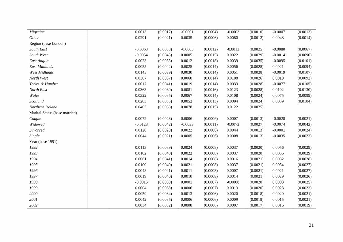
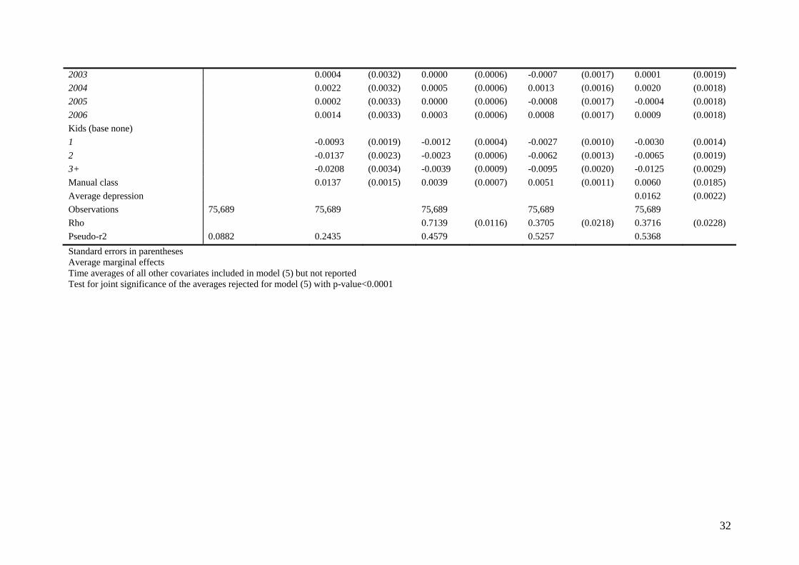
2003 0.0004 (0.0032) 0.0000 (0.0006) -0.0007 (0.0017) 0.0001 (0.0019) 2004 0.0022 (0.0032) 0.0005 (0.0006) 0.0013 (0.0016) 0.0020 (0.0018) 2005 0.0002 (0.0033) 0.0000 (0.0006) -0.0008 (0.0017) -0.0004 (0.0018) 2006 0.0014 (0.0033) 0.0003 (0.0006) 0.0008 (0.0017) 0.0009 (0.0018) Kids (base none) 1 -0.0093 (0.0019) -0.0012 (0.0004) -0.0027 (0.0010) -0.0030 (0.0014) 2 -0.0137 (0.0023) -0.0023 (0.0006) -0.0062 (0.0013) -0.0065 (0.0019) 3+ -0.0208 (0.0034) -0.0039 (0.0009) -0.0095 (0.0020) -0.0125 (0.0029) Manual class 0.0137 (0.0015) 0.0039 (0.0007) 0.0051 (0.0011) 0.0060 (0.0185) Average depression 0.0162 (0.0022) Observations 75,689 75,689 75,689 75,689 75,689 Rho 0.7139 (0.0116) 0.3705 (0.0218) 0.3716 (0.0228) Pseudo-r2 0.0882 0.2435 0.4579 0.5257 0.5368 Standard errors in parentheses Average marginal effects Time averages of all other covariates included in model (5) but not reported Test for joint significance of the averages rejected for model (5) with p-value<0.0001

Table VIII. Regression models containing area wage and unemployment effects Random-Effects dynamic and time averages Random-Effects dynamic and time averages

(with area wage and unemployment rates) Random-Effects dynamic and time averages (area specification sample excluding area rates)

Males Depressed 0.0040 (0.0019) 0.0011 (0.0024) 0.0010 (0.0024) IB claim past year 0.0486 (0.0025) 0.0529 (0.0039) 0.0531 (0.0039) Initially IB claim 0.0268 (0.0019) 0.0177 (0.0025) 0.0179 (0.0025) Area unemp. Rate 0.0019 (0.0006) Area wage rate 0.0022 (0.0081) Average depression 0.0352 (0.0034) 0.0383 (0.0043) 0.0383 (0.0043) Observations 69,436 39,644 39,446 Rho 0.3031 (0.0208) 0.2618 (0.0334) 0.2606 (0.0333) Pseudo-R2 0.5667 0.5820 0.5814 Females Depressed 0.0067 (0.0012) 0.0067 (0.0017) 0.0067 (0.0017) IB claim past year 0.0347 (0.0022) 0.0386 (0.0035) 0.0387 (0.0035) Initially IB claim 0.0261 (0.0016) 0.0209 (0.0022) 0.0209 (0.0022) Area unemp. Rate 0.0011 (0.0005) Area wage rate 0.0077 (0.0069) Average depression 0.0162 (0.0022) 0.0204 (0.0030) 0.0205 (0.0030) Observations 75,689 42,795 42,795 Rho 0.3716 (0.0228) 0.3648 (0.0351) 0.3631 (0.0350) Pseudo-R2 0.5368 0.5499 0.5495 Standard errors in parentheses Average marginal effects In addition to the area rates, the same covariates are included as those in the final models of Tables VI and VII but not reported. Test for joint significance of the averages rejected for all models with p-values<0.0001

Table IX. Regression models with GHQ caseness as the measure of depression Health Problems: Depression GHQ caseness Raw Pooled Random-Effects Random-Effects

dynamic and time averages

Raw Pooled Random-Effects Random-Effects dynamic and time averages

Males 0.1236 (0.0027) 0.0654 (0.0022) 0.0142 (0.0014) 0.0040 (0.0019) 0.0689 (0.0020) 0.0378 (0.0017) 0.0090 (0.0009) 0.0041 (0.0013) Depressed Average depression 0.0352 (0.0034) 0.0193 (0.0027) Observations 69,436 69,436 69,436 69,436 67,874 67,874 67,874 67,874 Rho 0.6890 (0.0127) 0.3031 (0.0208) 0.6984 (0.0125) 0.3143 (0.0211) Pseudo-R2 0.0746 0.3202 0.4769 0.5667 0.044 0.311 0.476 0.566 Females Depressed 0.0770 (0.0018) 0.0470 (0.0016) 0.0061 (0.0007) 0.0067 (0.0012) 0.0467 (0.0015) 0.0300 (0.0014) 0.0036 (0.0005) 0.0063 (0.0009) Average depression 0.0162 (0.0022) 0.0126 (0.0020) Observations 75,689 75,689 75,689 75,689 74,109 74,109 74,109 74,109 Rho 0.7139 (0.0116) 0.3716 (0.0228) 0.7224 (0.0112) 0.3702 (0.0229) Pseudo-R2 0.0882 0.2435 0.4579 0.5368 0.0428 0.2274 0.4540 0.5359 Standard errors in parentheses Average marginal effects Full range of covariates not reported Test for joint significance of the averages rejected for models (4) and (8) with p-values<0.0001 for both.

Figure 1

010

2030

Per

cent

-4000 -2000 0 2000 4000Contribution (£)

All claimants

010

2030

Per

cent

-4000 -2000 0 2000 4000Contribution (£)

IB claimants

Males

010

2030

Per

cent

-4000 -2000 0 2000 4000Contribution (£)

All claimants

010

2030

Per

cent

-4000 -2000 0 2000 4000Contribution (£)

IB claimants

Females

Contributions of less than -£3000 and those more than £3000 are excluded

Distribution of Contributions