Merging tidal datums and Lidar elevation for species distribution modeling in South San Francisco Bay Abstract: Because high tides increase in elevation across South San Francisco Bay, and because tidal inundation structures tidal salt marshes plant zonation, species distribution models (SDMs) of salt marsh plants require integrated, spatially continuous measures of tidal patterns and elevation. Continuous Lidar elevation data is available for South San Francisco Bay, but tidal datum values from National Ocean Service (NOS) tidal stations in the region are available only as point locations. In order to effectively normalize Lidar elevations to tidal heights, an interpolated data layer of tidal datums was created in ArcGIS. MHHW from 16 tide stations were extracted from tidesandcurrents.noaa.gov, translated to NAVD88 using a conversion table created by NOS for a 2005 hydrographic survey, then interpolated using the spline tool in ArcGIS. Then, the lidar elevation layer was subtracted from the MHHW layer, normalizing elevation relative to MHHW and creating an input meaningful for region wide marsh vegetation distribution models. Results and sources of error in the output are discussed. Introduction: Commonly used species distribution models, such as maximum entropy, or logistic regression models rely on meaningful environmental inputs to accurately predict species ranges (Phillips et al, 2004; Guisan and Zimmerman, 2000). In tidal marshes, while vegetation distributions depend on many factors including salinity, soil properties and competition, the single biggest predictor of marsh vegetation zonation is frequency and duration of inundation by the tides (Chapman, 1938; Hinde, 1954). Therefore, species distribution models and studies of South Bay marsh vegetation are likely to benefit from access to a raster layer which relates the interplay of tides and elevation across the South Bay. In the South Bay, frequency and duration of inundation by tides increase relative to a fixed geodetic datum the farther South one travels (Figure 1). This effect is amplified in the lower reaches of the South Bay as open water transitions to shallow shoals and channels (Waters et al, 1985). Addressing this regional inundation gradient, one author notes, “the tidal range is greater in the southern reach- 2.6 m at the southward boundary as compared to 1.7 m at the Golden Gate” (Conomos, 1979). And while the increase in the elevation of high tides is less pronounced in the North Bay than the South, the vertical range of salt marsh vegetation species in both reaches of the estuary respond to the change. Figure 1: Measures of average high tides increase relative to mean tide level in the San Francisco Bay Estuary with distance from the Golden Gate. This effect is amplified in the S. Bay due to tidal geometry (Conomos, 1979).
Transcript
Merging tidal datums and Lidar elevation for species distribution modeling in South San Francisco Bay
Abstract: Because high tides increase in elevation across South San Francisco Bay, and because tidal inundation structures tidal salt marshes plant zonation, species distribution models (SDMs) of salt marsh plants require integrated, spatially continuous measures of tidal patterns and elevation. Continuous Lidar elevation data is available for South San Francisco Bay, but tidal datum values from National Ocean Service (NOS) tidal stations in the region are available only as point locations. In order to effectively normalize Lidar elevations to tidal heights, an interpolated data layer of tidal datums was created in ArcGIS. MHHW from 16 tide stations were extracted from tidesandcurrents.noaa.gov, translated to NAVD88 using a conversion table created by NOS for a 2005 hydrographic survey, then interpolated using the spline tool in ArcGIS. Then, the lidar elevation layer was subtracted from the MHHW layer, normalizing elevation relative to MHHW and creating an input meaningful for region wide marsh vegetation distribution models. Results and sources of error in the output are discussed. Introduction: Commonly used species distribution models, such as maximum entropy, or logistic regression models rely on meaningful environmental inputs to accurately predict species ranges (Phillips et al, 2004; Guisan and Zimmerman, 2000). In tidal marshes, while vegetation distributions depend on many factors including salinity, soil properties and competition, the single biggest predictor of marsh vegetation zonation is frequency and duration of inundation by the tides (Chapman, 1938; Hinde, 1954). Therefore, species distribution models and studies of South Bay marsh vegetation are likely to benefit from access to a raster layer which relates the interplay of tides and elevation across the South Bay. In the South Bay, frequency and duration of inundation by tides increase relative to a fixed geodetic datum the farther South one travels (Figure 1). This effect is amplified in the lower reaches of the South Bay as open water transitions to shallow shoals and channels (Waters et al, 1985). Addressing this regional inundation gradient, one author notes, “the tidal range is greater in the southern reach- 2.6 m at the southward boundary as compared to 1.7 m at the Golden Gate” (Conomos, 1979). And while the increase in the elevation of high tides is less pronounced in the North Bay than the South, the vertical range of salt marsh vegetation species in both reaches of the estuary respond to the change.
Figure 1: Measures of average high tides increase relative to mean tide level in the San Francisco Bay Estuary with distance from the Golden Gate. This effect is amplified in the S. Bay due to tidal geometry (Conomos, 1979).
A number of studies have found that tidal salt marsh species distributions vary with the average elevation of high tides. Perhaps the most thorough longitudinal study of San Francisco Bay marsh vegetation found that high marsh plains are “typically situated 0.0 - 0.15 m above MHHW”, though the study also finds one marsh plains -.15 and another -.3 m below MHHW (Figure 2). Addressing the variability between high marsh elevations, the authors suggest that more recently formed tidal marshes are situated lower in the tidal frame and when mature reach an equilibrium elevation slightly above MHHW. (Atwater and Hegel, 1976)
Figure 2: Elevations of 6 high marsh plains along the northern reach of the SF Bay Estuary are situated within a few decimeters of MHHW (From Atwater and Hegel, 1976).
Other studies which have measured the vertical distribution of specific species in multiple marshes along the S. Bay reinforce this finding. While not specifically testing the effect of average high tides on species distribution, two separate data sets show that the vertical ranges of Spartina foliosa, Sarcocornia pacifica and Distichlis spicata (species representative of the low, mid and high tidal salt marsh in San Francisco Bay- see Hinde, 1954), each increase vertically at marshes further south in the S. Bay. This holds true whether species vertical distributions are measured relative to a vertically fluctuating tidal datum such as MLLW (Orlando, 1983) or a fixed geodetic datum such as NAVD88 (PWA and Faber, 2004). The idea that marsh vegetation trends with average high tides, and that predicting species distributions hinges on understanding how tides interact with elevation, is supported by tidal marsh restoration practice. A recent planning document for the South Bay Salt Pond Restoration Project at Pond A21 states that, “the relationship between pond elevations and tide heights is fundamental to the outcome of the [project]”. Furthermore, the project, now underway, successfully predicted vegetation would establish shortly after pond breach based on locally measured tidal datums and pond hydrographic survey data (USFWS and SCVWD, 2006). A planning document for nearby Pond A6 cited as the likely elevation of the future marsh plain MHHW, and specifies sections of an outboard levy surrounding the former salt pond be lowered to that elevation for the establishment of Sarcocornia pacifica (PWA, 2007). However, not all studies in the San Francisco Bay agree that inundation, considered alone, is a useful predictor of marsh elevation. In particular, the upland transition zone on the West Coast appears to vary considerably relative to tidal datums (Josselyn, 1983), though this review relies in part on studies that acknowledge that difficulty in accurately measuring tidal datums across their study range may have contributed to that finding (Frenkel, 1981).
And not all marsh species may trend primarily with the MHHW tidal datum. A recent study of the vertical range occupied by Spartina alterniflora x foliosa in S.F. Bay found that the invasive hybrid is more closely correlated to tidal range than variation in measures of tidal height (Collins, 2002), a result supported by studies of Spartina alterniflora on the East Coast (McKee, 1988). It’s worth noting here that MHHW and tidal range will be positively correlated so long as mean tide level remains constant or increases at the same time- which is true progressively south across the S. bay. Table 1: 10 factors operating in a salt marsh (Chapman, 1934)
It is well established that multiple factors influence salt marsh species zonation (Chapman, 1934; Table 1) and no one factor will explain all variability in spatial patterns. Indeed, any species distribution model seeking to predict vegetation patterns at the landscape scale across San Francisco Bay would be well advised to include salinity data, which is also known to structure marsh species distribution patterns and can affect inundation tolerance, and thus species vertical distributions in regard to tide levels (Atwater and Hegel, 1976). This study focuses on deriving one of many potential raster layers useful for species distribution modeling, a key ecological factor termed by Atwater and Hedel, “elevation with respect to tide level”. Based on literature reviewed for this study, the tide level of greatest utility in species distribution modeling may be the MHHW tide level, though interpolations of MHW, MLW, MSL, MLLW, and MN are also included, as these tidal datums may also be of use in vegetation studies in South San Francisco Bay. Methods: Overview: In order to derive a single raster layer representing the elevation of S. Bay tidal marshes with respect to the MHHW, the following analyses were performed. First, an elevation layer was derived from a 2004 Lidar survey made available through the San Francisco Estuary Institute. Next, tidal datum values and spatial locations of tide stations were extracted relative to MLLW from tidesandcurrents.noaa.gov and converted using a MLLW to NAVD88 conversion table from a 2005 hydrographic survey of South San Francisco Bay, then interpolated using ArcGIS 9.3.1. Next, the elevation and MHHW layers were arithmetically combined using raster calculator. Table 2: Data Sources: Elevation layer: San Francisco Bay 2004 Topographic Lidar
data set (Foxgrover, 2005) acquired through San Francisco Estuary Institute
Tidal datum point locations and values:
NOS tidal datums acquired from the Benchmark Sheet page at tidesandcurrents.noaa.gov
Tidal to geodetic datum conversion:
MLLW to NAVD88 conversion table from the 2005 NOS hydrographic survey of S. SF Bay (Foxgrover, 2007)
Elevation layer: The South San Francisco Bay 2004 Topographic Lidar data set (Foxgrover and Jaffee, 2005) was acquired from the San Francisco Estuary Institute in 2009 and used to create a 1-meter resolution digital elevation model (DEM) for analysis. Using ArcMap 9.3, Lidar ground return data was converted from xyz lattice files to multipoint features. Average point spacing was set to 1.2 meters. Multipoint features were converted to raster files, projected horizontally in NAD 1983 UTM Zone 10 and vertically in NAVD88. Tidal datum point locations and values: The National Ocean Service (NOS) and U.S. government predecessors have maintained tide gauges in San Francisco Bay since the first continuously operating water level monitoring station was installed in San Francisco in 1854 (Theberg, 2004). Tidal data from these gauges have been developed primarily for nautical charting and ship navigation tools (such as PORTS) as well as flood protection (USACE, 1984) but tidal datums from these stations have also been used many purposes including flood prediction (Knowles, 2008), and marsh vegetation studies (Hinde 1954, Atwater, 1979). 17 NOS water level monitoring stations from San Francisco to Gold Street Bridge (Figure 3) have tidal datums available within the current national tidal epoch (1983- 2001). These values were accessed using the interactive map available through tidesandcurrents.noaa.gov. Tidal datums relative to the MLLW tidal datum were extracted from the Benchmark Sheets page. Station location, station number, date of installation, date of removal, mean range and diurnal range were acquired from the Station Information page. Tidal range values, which are independent from any tidal datum, were extracted from the Datums page. These data were compiled into and Excel spreadsheet.
Figure 3: Tidal station data, including tidal datums were accessed using the interactive map at tidesandcurrents.noaa.gov. Tidal datum values were extracted from the Tidal Benchmark sheet where values are listed relative to the MLLW tidal datum.
Tidal to geodetic datum conversion: Tidal datums (Figure 4) are vertical references based on averages of tidal patterns over a 19 year tidal epoch. Because tides vary across the estuary, the absolute elevation of each tidal datum relative to a fixed geodetic datum, such as NAVD88, varies at each water leveling station. This means that each tide station requires a unique adjustment to convert tidal datums to NAVD88.
Ideally, to convert tidal datums relative to MLLW to tidal datums relative to NAVD88, each tide station gauge should be surveyed relative to a nearby tidal benchmark with a known absolute elevation, allowing a simple arithmetic conversion. This conversion is provided on the Benchmark Sheet page if a minimum of two tidal benchmarks connected to the same tide gauge have been surveyed as part of the National Geodetic Survey (NGS), and survey results place the benchmarks vertically within 9mm of each other. In these cases, the simplest and most reliable way to convert MLLW to NAVD88 is by using the adjustment provided by the NGS on the Benchmark Sheets page (Michael Michalski, personal communication, 2010). However, not all station gauges have tidal benchmarks that meet NGS standards. For these stations, the most reliable source to convert MLLW values to NAVD88, currently, is a conversion table created by a NOS 2005 hydrographic survey of S. San Francisco Bay (Anne Sturm, personal communication, 2010). The conversion table was created in order to convert bathymetry data measured relative to MLLW to NAVD88. The survey used existing NGS verified tidal benchmarks and updated additional tidal benchmark with GPS, then interpolated the MLLW to NAVD88 conversion factor across the study extent adjusting for changes in diurnal tide range (Foxgrover, 2007). The complete Foxgrover conversion table is provided in the Appendix, Figure 1 and Table 3. Therefore, in this study, at locations where NGS leveled gauges were available, tidal datum values relative to MLLW were converted to NAVD88 in Excel by subtracting the posted NAVD88 elevation from tidal datum values listed on the Benchmark Sheets page. Where NGS leveled gauges were not available the elevation conversion “NAVD88 above MLLW”
Figure 4: Tidal datums provide vertical references based on average tidal patterns. For example, elevations on nautical charts of San Francisco Bay are referenced relative to mean lower low water (MLLW).
(Appendix, Table 3, Foxgrover, 2007) was subtracted from tidal datum values on the Benchmark sheets page. The resulting Excel file with tidal datum values listed in NAVD88, with additional information extracted from tidesandcurrents.noaa.gov, is provided in the Appendix, Table 1. Vdatum for conversion to NAVD88 is not recommended in S. San Francisco Bay MLLW relative tidal datums were also converted to NAVD88 using the VDatum module (http://vdatum.noaa.gov/) to contrast with NOS conversion table results. Datum translations using VDatum are known to be particularly inaccurate in the S. Bay and the Foxgrover, 2007 conversion table is currently the recommended conversion (Anne Sturm, personal communication). To demonstrate the differences between Vdatum and NOS conversion factors, a single interpolation of MHHW values only was performed using Vdatum to convert MLLW values at non-NGS leveled tide stations. The conversion to Vdatum was performed using methods described at vdatum.noaa.gov. Interpolation of tidal station data: Spatial interpolation is fast and relatively accurate method of creating “tidal datum fields”. This can be accomplished by interpolating tidal constituents independently, or more simply by interpolating tidal values such as MHHW, MLLW, etc (Hess, 2002; Hess and Gill, 2003). Previously in San Francisco Bay, tidal datum values from NGS leveled tidal stations have been extracted from NOS tide stations and interpolated using a spine interpolator to create an input for a hydrodynamic numerical model to predict impacts of sea level rise in the Bay Area (Knowles, 2008). All interpolations (Table 3) were carried out using ArcGIS 9.3.1 using the spline interpolator with the following settings: tension, cell size = 10 meters, weight = .1, number of points = 12. The spline tool creates a surface that minimizes curvature but that passes through the source points and is often the best method for representing smoothly varying variables (Childs, 2004). The tension option uses more points than the regular option and usually results in a smoother surface. The analysis extent includes tidal stations outside of the lidar extent because these data points are significant in determining the trend of interest within the lidar extent. Slough geometry was not considered during interpolation. Table 3: Interpolations using the following data sources, number of stations and tidal datums relative to NAVD88 were performed for this study: Source of MLLW to NAVD88 conversion:
* The Alameda Creek station was included for comparison, but not used for further analysis because of anomalously low MHHW.
** No Vdatum conversion was available for Gold Street Bridge, but Alameda Creek and two additional stations near the central bay were included, for a total of 18 stations. The two central bay stations could not be included in NOS interpolations because NOS conversions were not available for those stations.
Of the 17 tide stations with tidal datum values, 16 tide stations were used for NOS converted interpolations of MHHW, MHW, MSL, MLW, MLLW and MN. These are the “best available data” based on this study. Alameda Creek station was removed because it has anomalously low values, and therefore was only included in only one interpolation (17 stations) to demonstrate the effect of inclusion and justify elimination. Additionally, one interpolation was carried out with Vdatum converted datum values to demonstrate differences between converting MLLW to NAVD88 with NOS conversion table vs. Vdatum. Normalizing elevation to tidal datums: Lidar ground elevations were subtracted on a cell by cell basis from the NOS/NGS leveled 16 station tidal datum interpolations of MHHW using raster calculator in ArcGIS at the cell size of the Lidar data (1 meter resolution). The resulting raster depicts elevation relative to the MHHW tidal datum layer. Results:
Lidar DEM:
Figure 5: Elevation DEM (1 m resolution) derived from 2004 Lidar data set (Foxgrover, 2005)
Interpolations of tidal station data: Datum field: MHHW Datum field: MHHW Datum source: NOS tidal stations Datum source: NOS tidal stations Conversion: Foxgrover, 2007 Conversion: Foxgrover, 2007 Stations included: 16 Stations included: 17 (w/ Alameda Creek)
Datum field: MHHW Datum field: MHHW Datum source: NOS tidal stations Datum source: NOS tidal stations Conversion: Foxgrover, 2007 Conversion: Vdatum Stations included: 16 Stations included: 18
Figure 6: Comparisons of MHHW interpolated tidal datum layers. The interpolation made using “best available data” (16 stations w/ NOS and NGS converted data) is shown twice (left side panels) for ease of comparison with MHHW interpolation results when Alameda Creek is included (top right) and when the MLLW- NAVD88 conversion is made using Vdatum (bottom right).
Datum field: MHW Datum field: MSL Datum source: NOS tidal stations Datum source: NOS tidal stations Conversion: Foxgrover, 2007 Conversion: Foxgrover, 2007 Stations included: 16 Stations included: 16
Datum field: MLW Datum field: MLLW Datum source: NOS tidal stations Datum source: NOS tidal stations Conversion: Foxgrover, 2007 Conversion: Foxgrover, 2007 Stations included: 16 Stations included: 16
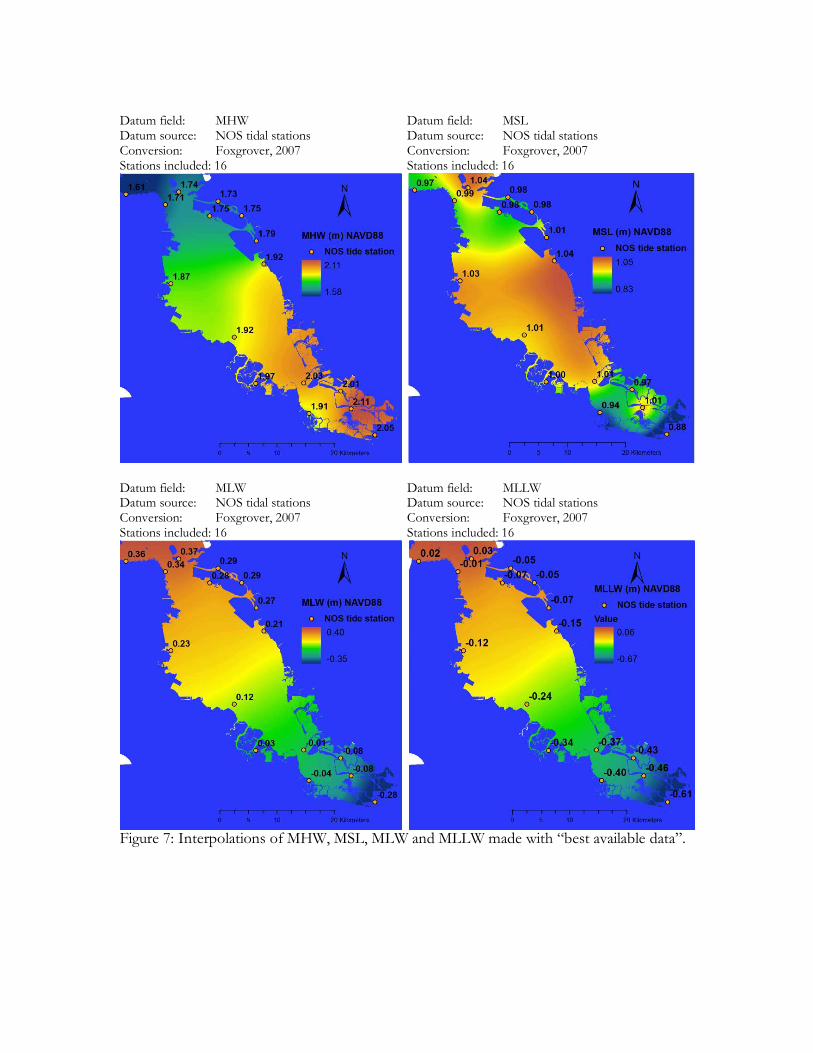
Figure 7: Interpolations of MHW, MSL, MLW and MLLW made with “best available data”.
Elevation normalized to MHHW:
Figure 8: Subtracting the Lidar elevation layer from the interpolated MHHW tidal datum field using raster calculator in ArcGIS results in Lidar elevations displayed relative to MHHW. Results are displayed here with interpolated MHHW tidal datum layer behind. Discussion: MHHW tidal datum interpolations: Interpolating using the best available data from 16 NOS and NGS adjusted tidal stations results in a MHHW tidal datum field that increases from 1.76 to 2.28 meters from the Golden Gate to Coyote Creek. This contrasts to Conomos, 1979 finding that tidal MHHW shifts from 1.7 to 2.6 meters across the same range. Interestingly, the MHHW interpolation made when the MLLW- NAVD88 conversion is made using Vdatum results in a MHHW
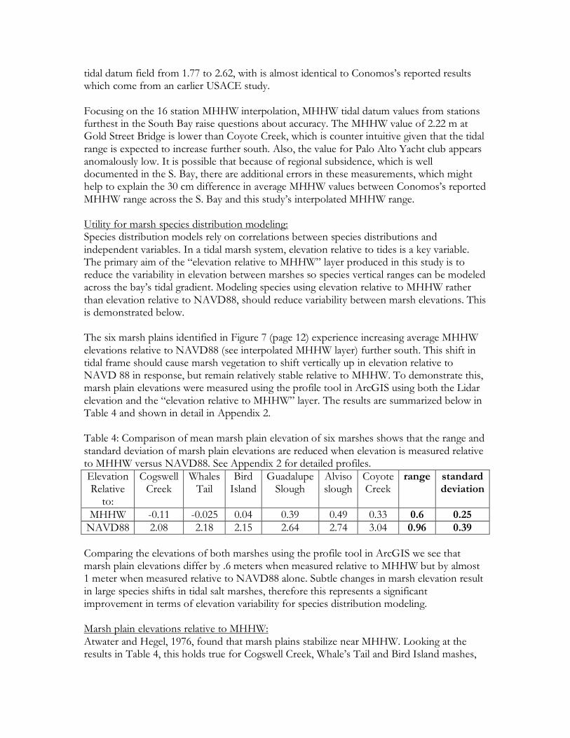
tidal datum field from 1.77 to 2.62, with is almost identical to Conomos’s reported results which come from an earlier USACE study. Focusing on the 16 station MHHW interpolation, MHHW tidal datum values from stations furthest in the South Bay raise questions about accuracy. The MHHW value of 2.22 m at Gold Street Bridge is lower than Coyote Creek, which is counter intuitive given that the tidal range is expected to increase further south. Also, the value for Palo Alto Yacht club appears anomalously low. It is possible that because of regional subsidence, which is well documented in the S. Bay, there are additional errors in these measurements, which might help to explain the 30 cm difference in average MHHW values between Conomos’s reported MHHW range across the S. Bay and this study’s interpolated MHHW range. Utility for marsh species distribution modeling: Species distribution models rely on correlations between species distributions and independent variables. In a tidal marsh system, elevation relative to tides is a key variable. The primary aim of the “elevation relative to MHHW” layer produced in this study is to reduce the variability in elevation between marshes so species vertical ranges can be modeled across the bay’s tidal gradient. Modeling species using elevation relative to MHHW rather than elevation relative to NAVD88, should reduce variability between marsh elevations. This is demonstrated below. The six marsh plains identified in Figure 7 (page 12) experience increasing average MHHW elevations relative to NAVD88 (see interpolated MHHW layer) further south. This shift in tidal frame should cause marsh vegetation to shift vertically up in elevation relative to NAVD 88 in response, but remain relatively stable relative to MHHW. To demonstrate this, marsh plain elevations were measured using the profile tool in ArcGIS using both the Lidar elevation and the “elevation relative to MHHW” layer. The results are summarized below in Table 4 and shown in detail in Appendix 2. Table 4: Comparison of mean marsh plain elevation of six marshes shows that the range and standard deviation of marsh plain elevations are reduced when elevation is measured relative to MHHW versus NAVD88. See Appendix 2 for detailed profiles. Elevation Relative
to:
Cogswell Creek
Whales Tail
Bird Island
Guadalupe Slough
Alviso slough
Coyote Creek
range standard deviation
MHHW -0.11 -0.025 0.04 0.39 0.49 0.33 0.6 0.25
NAVD88 2.08 2.18 2.15 2.64 2.74 3.04 0.96 0.39
Comparing the elevations of both marshes using the profile tool in ArcGIS we see that marsh plain elevations differ by .6 meters when measured relative to MHHW but by almost 1 meter when measured relative to NAVD88 alone. Subtle changes in marsh elevation result in large species shifts in tidal salt marshes, therefore this represents a significant improvement in terms of elevation variability for species distribution modeling. Marsh plain elevations relative to MHHW: Atwater and Hegel, 1976, found that marsh plains stabilize near MHHW. Looking at the results in Table 4, this holds true for Cogswell Creek, Whale’s Tail and Bird Island mashes,
but Coyote Creek, Alviso Slough and Guadalupe Slough Marshes are between .3 and .5 meters higher than MHHW datum layer. This result is likely associated with errors in Lidar data, raw tidal datum values, and interpolated datum values.
Figure 7: Six marsh plains were measured using the profile tool in ArcGIS to demonstrate reduced variability in marsh elevation using the “elevation relative to MHHW” layer, rather than if marsh plain elevations are measured relative to NAVD88. See Appendix 2 for detailed vertical profiles of each marsh. Sources of Error: A number of error sources are known to affect the results of this data layer, including error in LIDAR measurements, error in tidal datum measurements and errors in interpolation. Elevation error: Table 5: Error estimates of Lidar data over different terrain types.
2σ Error (cm) Terrain Description
+/- 10 – 15 Hard Surfaces (roads and buildings) +/- 15 – 25 Soft/Vegetated Surfaces (flat to rolling terrain) +/- 25 – 40 Soft/Vegetated Surfaces (hilly terrain)
Errors in Lidar data measurements are higher for vegetated marsh surfaces than flat hard surfaces, (Foxgrover, 2005) as shown below in Table 5. Furthermore, RTK GPS measurements in vegetated marshes frequently show a bias towards higher Lidar surface elevation measurements in dense vegetation- which is likely because ground points and vegetation points are more readily confused. Foxgrover discusses these errors in the 2005 report: “Lidar estimates of the bare earth surface in areas of pickleweed (salicornia virginica) marsh were good with a 2σ error of 18 cm while in the bulrush (Scirpus californicus or Scirpus maritimus), lidar performed poorly with a 2σ error of 192 cm. Based upon our limited number of bulrush ground-truth locations, we believe the high error is the result of the very dense vegetation that was impenetrable by the lidar.” This bias may account for the progressively higher marsh plain elevations in brackish marshes (Guadalupe Slough, Coyote Creek, Alviso Slough) which are dominated by bulrush.
Tidal datum error: Tidal datum errors are caused by the length of the time series (Table 6) used to calculate datum averages, the distance from primary tide stations, and measurement error. The Computational Technique for Tidal Datums Handbook (NOAA, 2003) describes these errors in more detail, but it is unlikely these errors contribute significantly to the observed increase in marsh elevations further south, since these errors are relatively small. Table 6: Estimated error in tidal datums based on series length.
Errors in tidal datum measurements are also associated with the reliability of leveled tidal benchmarks. If leveling is not recent, tide gauges may have moved vertically relative to benchmarks due to seismic activity and regional subsidence. Currently, the NGS does not employ a field staff and therefore the most likely updates of tidal benchmark locations are likely to come from the ongoing USACE Shoreline Project (Anne Strum, personal communication, 2010) Errors in tidal benchmarks are exacerbated by error by error in the Goid3 model, the geodetic model of the earth’s surface NAVD88 is based on, which is known to be relatively inaccurate for S bay (Anne Strum, personal communication, 2010). The degree to which this error impacts this study is unknown. Interpolation error: Interpolation errors also impact this study- particularly in sloughs in the South Bay. Tidal stations are located along major slough channels or along the open bay. MHHW datum values should continue to increase up channels and further south in the S. Bay, but because
of relatively low MHHW values at Gold Street Bridge and Palo Alto Yacht Harbor, interpolation results fail to capture this increasing MHHW trend in the S. Bay. This, combined with Lidar data error in dense vegetation likely explain why marsh plain elevations appear to increase relative to MHHW in the S. Bay marshes examined in Figure 7. Tidal datum interpolation validation Two known independent tidal gauges in the area are available to validate the tidal datum portion of this model. 1. Phillip Williams and Associates installed a temporary one-month water leveling station near pond A6 along Guadalupe Slough in the S. Bay. Using a vertical control established by Towill Inc., MHHW was measured at 7.37ft (2.24 m) NAVD88m. (PWA, 2007). The interpolated MHHW tidal datum layer used in this study is 2.25 m at this location. 2. A three month long tide series was collected near at railroad bridge in Coyote Creek. The gauge was leveled to a benchmark on the bridge which had been surveyed relative to NGVD29 and Vertcon was used to translate this value to NAVD88. MHHW was calculated to be 7.6 feet (2.32 m) NAVD 88 (USFWS and SCVWD, 2006). The interpolated MHHW tidal datum layer used in this study is 2.27 m at this location. This agreement between independent tidal datum measurements and the interpolated MHHW tidal datum layer suggests the tidal datum layer used in this model is accurate at the entrance to major tidal sloughs in the Coyote Creek/Guadalupe slough area. In conclusion, combining Lidar elevation with tidal datum values from NOS tide stations creates an elevation layer relative to MHHW that has less variability between marsh plain elevations and is therefore a more effective input for species distribution models than if elevation relative to NAVD88 were to be used alone. The resulting elevation relative to MHHW datum is more accurate for fully saline marshes in the central part of South San Francisco Bay then marshes in the brackish, southern part of San Francisco Bay where dense vegetation likely results in systematic Lidar errors falsely raising marsh elevations relative to MHHW. Installing tide stations in sloughs and channels in the S. Bay and updating the GEOG3 model and tidal benchmarks surveys would improve tidal datum layer interpolation accuracy. References: Ann Sturm, Personal Communication, 2010. Coastal Engineer, U.S. Army Corps of Engineers. Atwater, B. and C. W. Hedel, 1976. Distribution of seed plants with respect to tide levels and water salinity in the natural tidal marshes of the northern San Francisco Bay estuary, California. United States Department of the Interior Geological Survey, Menlo Park, Ca.Open-File Report 76- 389. Conomos, J. T., 1979. Properties and Circulation of San Francisco Bay Waters. Pacific Division of the American Association for the Advancement of Science c/o California Academy of Sciences Golden Gate Park San Francisco, California.
Chapman, V. J. 1934. The ecology of Scolt Head Island. In Scolt Head Island. Ed. J. A. Steers. Cambridge: W. Heffer & Sons, Ltd. 234 pp. Childs, C. 2004. Interpolating Surfaces in ArcGIS Spatial Analyst. ESRI Educational Servcies. Collins, J.N. 2002. Invasion of San Francisco Bay Smooth Cordgrass, Spartina alterniflora: A Forecast of Geomorphic Effects On the Intertidal Zone. San Francico Estuary Institute, Ca. Foxgrover, A. C., and B. E. Jaffe. 2005. South San Francisco Bay 2004 Topographic Lidar Survey: Data Overview and Preliminary Quality Assessment. U.S. Geological Survey Pacific Science Center, Santa Cruz, CA. Open-File Report 2005–1284 Foxgrover, A.C., Jaffe, B.E., Hovis, G.T., Martin, C.A., Hubbard, J.R., Samant, M.R., and Sullivan, S.M., 2007, 2005 Hydrographic Survey of South San Francisco Bay, California, U.S. Geological Survey Open-File Report 2007-1169 113 p. [URL: http://pubs.usgs.gov/of/2007/1169] Frenkel, R. E., Eilers, H. P., and C. A. Jefferson. 1981. Oregon Coastal Salt Marsh Upper Limits and Tidal Datums. Estuaries. Vol. 4:3 pp 198-205 Guisan, A. and N. Zimmerman. 2000. Predictive habitat distribution models in Ecology. Ecological modeling, Vol .135 pp147-186. Hess, K.W. 2003: Water level simulation in bays by spatial interpolation of tidal constituents, residual water levels, and datums. Continental Shelf Research. Vol. 23:5, 395-414. Hess, K. W. and S. K. Gill. 2002. Puget sound tidal datum by spatial interpolation. National Ocean Service, NOAA. 6.1. Hinde, H. P. 1954. The Vertical Distribution of Salt Marsh Phanerogams in Relation to Tide Levels. Ecological Monographs, Vol. 24:2, 209-225 Josselyn, M. 1983. The Ecology of San Francisco Bay Tidal Marshes: A Community Profile. U.S. Fish and Wildlife Service, Division of Biological Services, Washington, D.C. FWS/OBS-83/23. 102 pp. Knowles, N. 2008. Potential inundation due to rising sea levels in the San Francisco Bay region. California Climate Change Center. 31 pp. Michalski, Michael. 2010. Personal Communication. National Oceanic and Atmospheric Administration, National Ocean Service, and Center for Operational Oceanographic Products and Services, 2003. Computational Technique for Tidal Datums Handbook: NOAA Special Publication NOS CO-OPS 2. U.S. Department of Commerce. Silver Spring, Maryland.
Orlando, J. L., Drexler, J. Z. and K. G. Dedrick. 1983. South San Francisco Bay Tidal Marsh Vegetation and Elevation Surveys- Corkscrew Marsh, Bird Island, and Palo Alto Baylands, California, 1983: U.S. Geological Survey Data Series 134, 45 p. Phillips, S. J., Dudik, M., and R. E. Schapire. 2004. A maximum entropy approach to species distribution modeling. Proceedings of the 21st International Conference on Machine Learning, Banff, Canada. Phillip Williams and Associates, Ltd. and P. M. Faber. 2004. Design Guidelines for Tidal Wetland Restoration in San Francisco Bay. The Bay Institute. Appendix 1. Phillip Williams and Associates, Ltd. and H.T. Harvey and Associates. 2007. Alviso Pond A6 Tidal Restoration Preliminary Design Memorandum. Theberg, A. E. 150 years of tides on the western coast: The longest series of tidal observation in the Americas. NOAA Central Library. Accessed at http://tidesandcurrents.noaa.gov/pub.html US Army Corps of Engineers, 1984. San Francisco Bay Tidal Stage vs. Frequency Study. USACE San Francisco District. US Fish and Wildlife Service Don Edwards National Wildlife Refuge and the Santa Clara Valley Water District. 2006. Final Restoration and Mitigation Monitoring Plan for the Island Ponds Restoration Project.