at SciVerse ScienceDirect

Renewable Energy 48 (2012) 57e71

Contents lists available

Renewable Energy

journal homepage: www.elsevier .com/locate/renene

Mesoscale wind speed simulation using CALMET model and reanalysisinformation: An application to wind potential

Luis Morales, Francisco Lang*, Cristian MattarLARES (Laboratory for Research in Environmental Science), Department of Environmental Sciences and Renewable Natural Resources, University of Chile, Av. Santa Rosa 11315,La Pintana, Santiago, Chile

a r t i c l e i n f o

Article history:Received 28 November 2011Accepted 24 April 2012Available online xxx

Keywords:Wind fieldsSimulationNCEP-1CALMETWind potentialChile

* Corresponding author. LARES, Departamentoy Recursos Naturales Renovables, Universidad de CBox: 1104, La Pintana, Santiago, Chile. Tel.: þ56 2 978

E-mail address: fcolang@renare.uchile.cl (F. Lang).

0960-1481/$ e see front matter � 2012 Elsevier Ltd.doi:10.1016/j.renene.2012.04.048

a b s t r a c t

This work presents a simple methodology to simulate the mesoscale wind field using dynamic modelingand complementarymeteorological data.Meteorological information obtained from the project developedby theNational Center of Environmental Research (NCEP) and theNational Center of Atmospheric Research(NCAR), meteorological stations, a digital elevation model and a land use data were used in this study. Allthese datawere input for the simulation of wind fields at three different heights (20, 30 and 40m) throughthe CALMET model. Simulations were made for an area corresponding to the south central region of Chile,known as the Maule Region. The results show that the simulated spatial resolution (1 � 1 km) in theCALMETmodel yields good results, yielding an RMSE value near 1m s�1 for all the heights simulated, witha greater RMSE at 40 m (1.15 m s�1) and a lesser RMSE at 20 m (1.10 m s�1). The direction of the simulatedwind fieldswas also evaluated, yielding an RMSE near 31� at 40m. The determination of thewind potentialis presented as a direct application of the method shown in this work.

� 2012 Elsevier Ltd. All rights reserved.

1. Introduction

Wind speed is the most important meteorological variable fordetermining wind potential. In effect, wind energy is based on thedetermination of wind fields to determine their potential. Spatialand temporal variability are also measured across layers of theatmosphere near the surface. This is why the determination of windfields holds particular interest in the development of renewableenergy sources, as is the case of wind power, which has experi-enced significant growth over the last two decades and has becomea sustainable, reliable and efficient energy source [1]. However, themain barriers that arise when addressing the concept of windpotential are related to wind variability and the technical difficultyof identifying areas with good wind conditions [2]. The firstobstacle comes from the fact that wind is considered one of themost difficult meteorological variables to model and predict due toits dependence on the specific characteristics of any given location,such as topography and surface roughness [3]. The second is relatedto surface coverage, mainly to the classification and definition of an

de Ciencias Ambientaleshile, Av. Santa Rosa 11315,586; fax: þ56 2 9785929.

All rights reserved.

area with high or low wind potential, which requires analysis ofspatial and temporal variations in the speed and direction ofthe wind in a specific location and the vertical profile of the windspeed [4].

The most commonway of characterizing wind speed is throughin-situ measurements, which are not always available to thedesired extent and only allow a specific point determination of themagnitude and direction of the wind [5]. In addition, use of thesemeasurements is a major obstacle in developing countries, whichdo not have a dense network of meteorological stations [6]. Asa result, the most commonway to characterize the wind spatially isto interpolate point-specific measurements. However, this methodhas limited validity because, in many cases, interpolation can onlybe performed when the characteristics of the landscape areuniform and there is a dense distribution of wind speed measuringstations [7]. Therefore, a possible solution for the determination ofthe magnitude and direction of wind fields is utilization of differenttypes of simulations, depending on the desired spatial resolution ofthe results, the number of in-situ measurements (meteorologicalstations), and the complexity of the landscape (topography androughness of the surface), among others [8].

Themodels that allow simulation of wind fields are based on theintegration of information from field measurements, land use data,a digital elevation model, and complementary information, suchas vertical wind profiles, among others. For instance, there are

L. Morales et al. / Renewable Energy 48 (2012) 57e7158

different models, which differ in characteristics such as numericalformulation, assumptions, equation simplifications and type(diagnostic and prediction model). Prediction models solve theequations describing the atmospheric process and how the atmo-sphere changes with time [9]. Examples of these prediction modelsare MM5 [10], WRF [11], HIRLAM [12], and HRM [13]. On the otherhand, diagnostic models represent the actual state of the atmo-sphere [14] (Hu et al., 2010). Examples of diagnostic models areAERMET [15], MCSCIPUF [16] and CALMET [17]. Other models usedin wind energy assessment were analyzed in [18] and [19]. One ofthese models with interesting features is CALMET, which is a freedistribution model that generates wind fields over complex terrain.

The precision of the simulation of wind fields, in CALMET,depends in large measure on the quality and quantity of in-situmeasurements that are input into the model and on their spatialdistribution [20,21], which makes it necessary to have differentinformation sources to minimize sources of error. This integrationof meteorological observations from different sources and atdifferent resolutions (spatial or temporal) can come from satellitedata or low-resolution global databases [22]. Within this context,one database meets these requirements is the NCEP/NCAR Rean-alysis project (here-in-after NCEP-1), which was created in 1948 bythe National Center of Environmental Prediction (NCEP) and theNational Center of Atmospheric Research (NCAR). The availabledata represent global grids or meteorological information ondifferent variables including wind speed, thus permitting spatialinformation to be obtained that complements data from meteoro-logical stations for the CALMET simulation.

Both the NCEP-1 data and the CALMET model have beenpreviously used for studies of wind as a resource. In the case ofNCEP-1, the data have been used to visualize wind conditions inCanada [23,24] and also to develop the Wind Atlas Analysis andApplication Program (WAsP), of the Risø National Laboratory ofDenmark, which includes an extreme wind atlas [25]. CALMET hasbeen used in combination with forecast models and has yieldedgood results for more detailed resolution of the evaluation of windresources, for example with MM5 [22,26] or WRF [27,28]. This isbecause the model is suited to work on complex terrain [29] andlong-term simulations [30].

The goal of this work is to present a simple method to simulatewind fields with data from the NCEP-1 project and the CALMETmodel. As an application of this methodology, the wind potential ofan area in south central Chile, known as the Maule Region, thatexhibits complex terrain with few meteorological stations wasdetermined. This article is structured as follows: Section 2 describes

Fig. 1. Study area and location of the meteorological stations used in this work (b

the study area, the meteorological stations used and presents themain characteristics of the CALMET model and the NCEP-1 data-base. Section 3 presents the simulation methodology for the windfields, its evaluation and the determination of the wind potential.Section 4 shows the results obtained from the model, the evalua-tion of data from a meteorological station, the wind potential mapsand limitations of the proposed method. In addition, this sectionpresents the analysis of these results, and, finally, section 5 presentsthe conclusions of this study.

2. Study area and data set

2.1. Study area and in-situ measurements

The study area covers the south central region of Chile, knownas theMaule Region. This area is located between 34�410 and 36�330

south latitude and 70�180 and 72�450 west longitude, with a surfacearea of 30,269.1 km2. The weather in this region is a typicalMediterranean semiarid climate, with a mean temperature of17.1 �C between September and March (spring and summer). Themean annual precipitation in this region is approximately 676 mm,mainly concentrated during the winter months. The summerperiod is generally dry and hot (2.2% of the annual precipitation),whereas the spring is wetter (16% of the annual precipitation) [31].In-situ measurements from five meteorological stations were usedin this work. The measurements consisted of hourly records of themagnitude and direction of the wind. Fig. 1 shows the study areaand the location of the meteorological stations.

Of all the stations, four were used as inputs for the modelingperformed in CALMET. Two of these correspond to the Pahuil (35�

360 S. e 72� 340 W., 52 m.a.s.l.) and Putú (35� 120 S. e 72� 160 W.,8 m.a.s.l.) stations managed by the Dirección Meteorológica deChile, with a recording period between May and October of 1992.The other two stations correspond to the meteorological station ofthe Cauquenes Experimental Center of the INIA (Instituto deInvestigaciones Agropecuarias) (35� 580 S.e 72� 170 W.,140m.a.s.l.),with a recording period between the years 2003 and 2005, and thePanguilemo experimental station (35� 230 S. e 71� 400 W.,102 m.a.s.l.) of the University of Talca, with a recording periodbetween 2003 and 2006. The measurements performed by thesefour stations correspond to a height of 10 m. The remaining stationis Faro Carranza (35� 320 S.e 72� 350 W., 21 m.a.s.l), which was usedfor evaluation of the modeling. This station provides wind speedmeasurements at 20, 30 and 40 m and wind direction at 40 m, withdata records between January 29, 2006 and June 8, 2007. The area

lack triangles) superimposed on a digital elevation model of the same region.

Fig. 2. Flow chart of the calculation of the wind fields.

L. Morales et al. / Renewable Energy 48 (2012) 57e71 59

in which this meteorological station is located is known as PuntaCarranza is considered one of the sections most representative ofregional patterns. The location exhibits a wind direction predomi-nantly from the S and SW, which is consistent with the datarecorded by the Faro Carranza station and the results obtained fromthe CALMET simulation [32]. Table 1 summarizes the technicalcharacteristics of the stations used in this work.

2.2. Reanalysis information

Two data sets were configured as a grid of wind fields given bysub-daily data (four times a day), provided as the u (horizontal) andv (vertical) components of the wind (m s�1) given by the NCEP-1[33,34]. One of the data sets consists of surface information(10 m) of the speed and direction of the wind, whereas the otherconsists of information of the wind at the 1000, 925, 850, 700, 600and 500 HPa, according to the limitation that CALMET only usesdata up to 500 HPa in its model. These data correspond to a globalgrid of 2.5� � 2.5� latitude-longitude between January 1, 1948 andthe present. However, this work used data corresponding to theperiod between 1977 and 2006. These last 30 years were used toobtain themean climate behavior at the sub-daily level in the studyarea.

2.3. Land surface data

The CALMET model uses a terrain with complex topography ineach simulation of the wind fields. In general terms, CALMET usesthe GTOPO30 digital elevation model, which has a spatial resolu-tion of 1 � 1 km. This model was developed by the United StatesGeological Survey’s EROS Data Center. The type of land use is alsoa significant variable in the simulations performed by CALMET. Inthis case, the model uses the Global Land Cover Characterization(GLCC) database, which was developed by the U.S. GeologicalSurvey (USGS), the University of Nebraska-Lincoln (UNL), and theEuropean Commission’s Joint Research Centre (JRC). These data areavailable in the data set on the webpage of the CALMET model [35].

2.4. CALMET meteorological model

CALMET is a diagnostic meteorological model originally devel-oped by the California Air Resources Board and later improved bythe U.S. Environmental Protection Agency (EPA). The goal ofCALMET is to provide a simulation of wind fields that will be usedafterward in a pollutant dispersion model known as CALPUFF [17].

A series of variables is required for the CALMET model toperform a wind field simulation, such as wind observations at thesurface level (hourly temporal resolution) integrated with an inputof surface information, vertical profiles of the atmosphere (at leasttwo times a day) structured in a database of heights, and topo-graphic and land use information, structured in a geophysical datafile.

The CALMET model uses two steps for the calculation of windfields. In the first step, the observations configured in the surfaceinput are adjusted for kinematic effects of terrain, such asmountain-valley breeze effects, flow due to slopes and blocking

Table 1Summary of the characteristics of the meteorological stations.

Station name Latitude S Longitude W m.a.s.l. [m]

Pahuil 35� 360 450 ’ 72� 340 020 ’ 52Putú 35� 120 340 ’ 72� 160 540 ’ 8Cauquenes 35� 580 020 ’ 72�170 000 ’ 140Panguilemo 35� 220 120 ’ 71� 350 400 ’ 102Faro Carranza 35� 320 32" 72� 350 20" 21

effects (thermodynamic blocking effect of the terrain on airmovement), ending with calculation of the minimum divergence ofthe winds [17]. For the second step, the data of the observations areinput into thewind field obtained from step 1. In this procedure, theobservations are interpolated by the inverse square of the weighteddistance (Eq. (1)), giving more weight to the nearness of theobservation points.

ðu; vÞ02 ¼

ðu; vÞ1R2

þXk

ðuobs; vobsÞkR2k

1R2

þXk

1R2k

(1)

where (uobs, vobs)k are the observed wind components at station k(m s�1), (u,v)1 are the step 1 wind components at a particular grid

Start of sampling End of sampling Anemometer height [m]

28-04-1992 16-10-1992 1028-04-1992 16-10-1992 1001-01-2003 31-12-2005 1001-01-2003 31-12-2006 1029-01-2006 21-07-2008 20, 30 and 40

Table 2Classes of wind potential density.

Class Density of wind potential (W m�2) Viability

1 0e200 Very poor2 200e300 Poor3 300e400 Marginal4 400e500 Good5 500e600 Very good6 >600 Excellent

Source: State Energy Conservation Office.

L. Morales et al. / Renewable Energy 48 (2012) 57e7160

point (m s�1), (u,v)20 are the initial step 2 wind components (m s�1),Rk is the distance from observational station k to the grid point (m),and R is the weight parameter for the winds calculated in step 1.Next, a vertical extrapolation of the surface wind observations isperformed according to the power law (Eq. (2)).

uz ¼ um

�zzm

�p

(2)

where z is the height (m) of the middle point of the grid cell, zm isthe height (m) at the measurement height of the surface windobservation (typically 10 m), um is the component of the wind(m s�1) measured at height zm, uz is the extrapolation of thecomponent u of the wind (m s�1) at height z, and p is the exponent

Fig. 3. Flow chart of the methodology

of the power law. The same equation is applied to the other hori-zontal component v of the wind. The typical values for the expo-nent p of the power law are given by the CALMET model accordingto Douglas and Kessler [36], where the value of p is 0.143 on theground and 0.286 over water.

Subsequently, discontinuities are reduced in the horizontalwind fields, and the vertical velocities are fitted according to theprocedure described by O’Brien [37]. At the end of each step, thecontinuity equation is verified throughout the entire volume,verifying the minimum divergence of the winds in each cell, asshown by Eq. (3).

dudx

þ dvdy

þ dwdz

< ε (3)

where u and v are the horizontal wind components (m s�1),w is thevertical velocity (m s�1), and ε is the maximum allowable diver-gence. Fig. 2 summarizes the CALMET steps through a flow chart.

3. Methodology

3.1. Data processing

Before inputting the data to the CALMETmodel, it was necessaryto pre-process the NCEP-1 data and the meteorological stations to

used to determine wind potential.

Fig. 4. Mean monthly wind speed for the Maule region at a height of 10 m.

L. Morales et al. / Renewable Energy 48 (2012) 57e71 61

Fig. 4. (continued).

L. Morales et al. / Renewable Energy 48 (2012) 57e7162

Table 3Statistical results (in m s�1) of the simulation of wind speed with CALMET for 10 and40 m.

10 m 40 m

Min. Max. Mean SD Min. Max. Mean SD

January 1.60 10.26 4.59 1.01 1.95 12.52 5.60 1.24February 1.48 9.84 4.43 1.01 1.80 12.01 5.40 1.23March 1.42 8.86 4.00 0.94 1.73 10.80 4.88 1.14April 1.41 7.80 3.66 0.75 1.72 9.51 4.47 0.92May 1.23 8.67 4.11 0.78 1.50 10.58 5.01 0.95June 0.85 8.62 4.14 1.04 1.04 10.52 5.06 1.19July 0.88 8.68 4.22 1.26 1.07 10.59 5.15 1.40August 1.36 8.65 4.17 0.94 1.66 10.55 5.09 1.18September 1.39 8.04 3.81 0.75 1.70 9.80 4.73 0.91October 1.54 8.29 3.88 0.85 1.87 10.11 4.73 1.03November 1.46 8.30 4.08 0.94 1.78 10.89 4.98 1.15December 1.52 9.87 4.42 1.00 1.86 12.03 5.39 1.23Total 1.34 8.82 4.13 0.94 1.64 10.83 5.04 1.13

L. Morales et al. / Renewable Energy 48 (2012) 57e71 63

configure the surface meteorological data file. To optimize thesimulation process in CALMET, a representative area greater thanthe study areawas selected for the data fromNCEP-1 (at the surfaceand profile levels), covering a 10 � 10 adaptive kernel. To thisadaptive window, Kriging was applied with a linear variogram,generating a new grid with dimensions of 0.5 � 0.5� latitude-longitude. Once the data had been re-gridded, a temporal inter-polation of every 6-h period (sub-daily data) was made to obtainhourly data, because this is a mandatory requirement of theCALMET model. Accordingly, the cubic spline segmented interpo-lation method was used, yielding hourly data of wind speed anddirection. This interpolation uses a vector of point [xi,yi](i ¼ 0,1,.,n) with a continuous curve by parts that passes througheach of the values of the following equation:

SiðxÞ ¼ aiðx� xiÞ3þbiðx� xiÞ2þciðx� xiÞ þ di x˛½xi; xiþ1� (4)

where ai, bi, ci and di are coefficients and S(x) is the spline cubicinterpolation function. Finally, the hourly climatologic mean valueof the 30-year period was calculated, yielding 8760 hourly meanscorresponding to a mean year. This informationwas combined withdata from the four meteorological stations, and input files forCALMET were structured. For the vertical profile of wind speed, theinput file was structured only with the sub-daily data from NCEP-1.Finally, the values used for the land surface data were obtainedfrom the webpage of the CALMET model [35].

3.2. Wind field simulations and evaluation

CALMET was used for the simulation of the wind fields at anhourly frequency for one average year. To this end, the study areawas configured in a spatial domain of 265 columns by 235 rowswith a grid width of 1 km both in x (longitude) and in y (latitude)with 5 height layers of 10, 20, 30, 40 and 50 m. The first heightrepresents the measurement at the same height as the input fromthemeteorological stations. The following three heights (20, 30 and40 m) were selected to evaluate the modeling with data froma meteorological station that was not included in the model. Thechoice of a height of 50m is due to common use of this height valuefor the calculation of wind potential as shown in several studies,such as those by Refs. [23,24,38].

The data input to themodel at the surface level correspond to theNCEP-1 data combined with those from the complementary mete-orological stations (at an hourly time resolution). In the verticalprofile, the NCEP-1 data were input four times a day. As a final step,a digital model of vertical terrain elevation corresponding toGTOPO30 (1 km) and a land use map at the same spatial resolutionwere input (The Global Land Coverage Characterization, GLCC).These last two are enabled for automatic reading in CALMET.

To evaluate the results obtained in the simulation of wind fieldswith CALMET, a meteorological station not included in themodeling was used to compare the simulated results with in-situobservations. The Faro Carranza meteorological station wasselected for this purpose. The data obtained at this station for thethree heights (20, 30 and 40 m) were used for comparison with thespeed and direction of the wind simulated by CALMET. The statis-tical parameter used for the evaluation was the root mean squareerror (RMSE), which is defined as:

RMSE ¼"1N

XNi¼1

ðoi � eiÞ2#1=2

(5)

where oi is the wind speed (m s�1) at the Faro Carranza station, ei isthe wind speed (m s�1) yielded by the simulation, and N is the totalnumber of data points.

3.3. Wind potential determination

Starting from the simulated wind fields at 50 m, the windpotential was determined. This wind potential was calculated usingWeibull’s probability density function, which experimentallyapproximates the probability density curve of the wind and yieldsa good representation of the variation of the mean hourly windspeed at many locations [6,39,40]. The success of Weibull’s distri-bution function, expressed in Eq. (6), is based on the fit of twoparameters, which can give great flexibility in the distributionfunction of the measured values with different behavior [38].

f ðvÞ ¼ kc$�vc

�k�1exp

h��vc

�ki(6)

where v is the wind speed, c (m s�1) is theWeibull scale parameter,and k (dimensionless) is the form parameter that characterizes theasymmetry of the probability function.

There are several methods to determine these parameters (k andc). Using the method proposed by [41], the maximum probabilitywas calculated for data in the wind time series format. This methoduses the mean and the standard deviation to determine the k and cparameters with the following approximations:

k ¼�sv

��1;086ð1 � k � 10Þ (7)

c ¼ v

Gð1þ 1=kÞ (8)

where v (m s�1) is themeanwind speed, s is the standard deviation,and G is the Gamma function, which is defined by the followingequation [38]:

GðxÞ ¼ZN0

tx�1expð�tÞdt (9)

Once the wind speed distribution was known, the wind poten-tial was determined [38] by the following equation.

PðvÞ ¼ 12rv3 (10)

where v (m s�1) is the wind speed, and r (kg m�3) is the density ofair. At standard conditions of 1 atm and 15 �C, the density of air is1.225 kg m�3 [42]. The surface units are given by the areaperpendicularly exposed to the flow of the wind.

L. Morales et al. / Renewable Energy 48 (2012) 57e7164

Keeping in mind that the wind speed varies over time, anadequate characterization of the available wind potential must takeinto account the potential values of each wind speed. Accordingly,these speeds must be averaged over a determined time period. Thiscan be expressed by the following equation:

PðvÞ ¼ 12r

ZN0

v3f ðvÞdv (11)

Fig. 5. Mean monthly wind speed for th

where f ðvÞ is Weibull’s probability density function given by Eq. (6).Eq. (11) yields the maximum available wind potential at a deter-mined site.

Once the wind potential estimate was determined, a classifica-tion was made of different wind potential densities following thecriteria of the Texas State Energy Conservation Office [43], whichestablishes qualitative magnitudes of the availability of the windresource shown on Table 2. Fig. 3 shows a flow chart of the meth-odology presented in this section.

e Maule region at a height of 40 m.

L. Morales et al. / Renewable Energy 48 (2012) 57e71 65

4. Results and analysis

4.1. Wind field simulations

Fig. 4 shows the monthly mean of the wind speed at a height of10 m for one year. It can be seen that the maximum speed areassociated with mountainous sectors, which contrast in magnitudewith the wind speed values obtained for flat sectors. The flat areasdisplay the minimum values of the wind fields for the entiresimulated time range. Table 3 shows the mean, standard deviation,and the monthly minima and maxima. The month with the highest

Fig. 5. (cont

mean speed is January, with a maximum of 10.3 (m sec�1). Incontrast, April is the month with the lowest speed, havinga maximum of 7.8 (m sec�1). Fig. 5 shows the wind fields at a heightof 40 m. The figure also shows that the mean wind speed in somemountainous sectors surpasses 10 m s�1 for most of the year. Inaddition, it is seen that high speed are not only associated withmountains east, but also with mountainous sectors to the west ofthe region. At this height, the maxima also reach 12.5 (m sec�1) forthe month of January. For both heights, in the hourly determinationof the wind characteristics, it is possible to see that there aremarked seasonal periods that are mainly due to different synoptic

inued).

Fig. 6. Hourly comparison between the results of the model and the Faro Carranza station for three heights: (a) 20 m, (b) 30 m and (c) 40 m.

L. Morales et al. / Renewable Energy 48 (2012) 57e7166

factors that exist during the summer, such as the influence of highpressures and of the Pacific anticyclone, which produces anincrease in wind speed with maxima for the month of January andminima for the month of April. For the winter months (June, July,

Table 4Statistical results (in m s�1) of the comparison between thewind speed simulated by CALMmonthly mean for the heights of 20, 30 and 40 m. N ¼ 8760.

20 m 30 m

Bias s RMSE Bias s RM

January �1.6 � 10�3 1.18 1.18 �1.1 � 10�3 1.21 1.2February �4.3 � 10�4 0.93 0.93 �1.9 � 10�3 0.97 0.9March �7.4 � 10�4 0.89 0.89 �3.0 � 10�4 0.93 0.9April �4.1 � 10�4 0.83 0.83 �2.0 � 10�4 0.86 0.8May �3.4 � 10�4 0.77 0.77 9.2 � 10�4 0.88 0.8June �2.1 � 10�3 1.06 1.06 �1.4 � 10�4 1.16 1.1July �1.2 � 10�3 1.50 1.50 �2.1 � 10�3 1.56 1.5August �2.3 � 10�3 1.20 1.20 �1.7 � 10�3 1.25 1.2September �2.0 � 10�3 0.83 0.83 �9.1 � 10�4 0.88 0.8October �6.3 � 10�4 1.01 1.01 �1.5 � 10�3 1.05 1.0November 8.9 � 10�4 0.98 0.98 �1.6 � 10�3 1.06 1.0December �2.4 � 10�3 1.21 1.21 �2.7 � 10�3 1.37 1.3Total �1.1 � 10L3 1.03 1.03 L1.1 � 10L3 1.10 1.1

August), the region is exposed to sporadic frontal storms, which area product of baroclinic instability [44]. This effect is reflected inoccasional increases in the wind speed that generate a higher meanvalue of wind speed.

ETand the values recorded for each height at Faro Carranza. The results are shown at

40 m Total

SE Bias s RMSE Bias s RMSE

1 �2.2 � 10�3 1.34 1.34 �1.6 � 10�3 1.24 1.247 �1.3 � 10�3 0.95 0.95 �1.2 � 10�3 0.95 0.953 �1.9 � 10�3 0.95 0.95 �9.9 � 10�4 0.92 0.926 �1.2 � 10�3 0.88 0.88 �6.1 � 10�4 0.86 0.868 �4.1 � 10�4 0.90 0.90 6.1 � 10�5 0.85 0.856 �1.5 � 10�3 1.16 1.16 �1.3 � 10�3 1.13 1.136 1.1 � 10�3 1.71 1.71 �7.3 � 10�4 1.59 1.595 �2.3 � 10�3 1.35 1.35 �2.1 � 10�3 1.27 1.278 �3.2 � 10�4 0.97 0.97 �1.1 � 10�3 0.89 0.895 �1.7 � 10�3 1.14 1.14 �1.3 � 10�3 1.07 1.076 �3.4 � 10�4 1.13 1.13 �3.3 � 10�4 1.06 1.067 �2.3 � 10�3 1.37 1.37 �2.5 � 10�3 1.32 1.320 L1.2 � 10L3 1.15 1.15 L1.1 � 10L3 1.09 1.09

Fig. 7. Polar diagrams for (a) Faro Carranza and (b) the simulation.

Table 5Statistical results (in degrees) of the comparison between the direction of the windsimulated by CALMETand the records observed for each height at Faro Carranza. Theresults are shown at the monthly mean for a height of 40 m.

40 m

Bias s RMSE

January 10.4 28 30February 10.1 31 32March 5.4 33 33April 2.0 30 30May 1.3 30 30June 2.9 26 26July 2.3 26 26August 4.1 28 29September 2.8 32 32October 1.8 32 32November 5.5 34 34December 6.9 32 33Total 4.6 30 31

L. Morales et al. / Renewable Energy 48 (2012) 57e71 67

For the wind direction, the movement patterns are similar forthe two heights. During the summer months (December, Januaryand February), the winds with a northeasterly direction prevail. Incontrast, during the winter months (June, July and August),southwesterly winds prevail. At both 10 and 40 m, the influence ofthe mountains in this sector of the study area permits observationof the variations and channeling patterns of air that result from thelocal topography. In contrast, the central valleys and the coastalmountainous sector exert less influence on the air flows.

4.2. Evaluation of modeling

The comparison of the simulated time series at the hourlylevel with the data from the Faro Carranza meteorological stationis presented in Fig. 6. In the case of the wind speed, the annualbehavior of the simulation for the three heights has a high degreeof similarity with the patterns from the Faro Carranza station,with a mean determination coefficient of 0.85. The similarity ofthe maxima during the winter months of June, July and Auguststands out. In general, the simulated values are greater than thevalues from the meteorological station, with differences of up to7 m s�1 at 40 m in the winter months. Table 4 shows the errorsobtained when comparing the simulated wind magnitudes withthe Faro Carranza station. These results are shown for each heightand for the entire time range for which this station recorded data.A bias is revealed, with negative values for the three heights andfor all months, that indicates that the CALMET model over-estimated the resulting wind magnitudes. The RMSE values rangefrom 0.77 m s�1 in the month of May at 20 m to 1.71 m s�1 in themonth of July at 40 m, with a mean of 1.09 m s�1 Fig. 7(a) and (b)shows the polar diagram for the measured and simulated winddirections. It can be seen that the direction of the wind is similaramong the observations and simulations, where the NNWdirection is the least common in both cases. In contrast, the SSWdirection is most common for Faro Carranza, whereas the Sdirection is most common for the simulation. The percentage ofcalms was 4.2% for Faro Carranza and 0.16% for the CALMETsimulation. Table 5 shows the statistical results, in which theRMSE ranges between 26 and 34�.

4.3. Wind potential determination

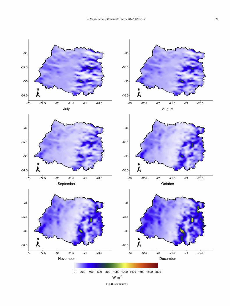
Fig. 8 shows the density of the monthly mean wind potential ataheightof50mcalculatedwithEquation(11),which incorporates the

distribution of the wind speed, allowing determination of the varia-tion in thewindpotential resulting fromdailycycles [45]. Themaximaduring theyearfluctuate between725and2062Wm�2,with Januaryhaving the highest potentials. High values were observed on themountain tops, which is in agreement with thewind fields obtained.Coastal sectors also standout,withpotentials that rangebetween300and 680Wm�2 and are associated with the hills present in the area.The central valleys, mountain valleys and canyon depths have lowpotentials throughout all the months of the year.

The density classes ofwindpotential for 50mare showed in Fig. 9.The central zoneof the studyareawas classifiedashaving “verypoor”wind availability, preventing the development of wind energy in thissector, which agrees with the fact that this zone has the lowest windspeed. Mountainous sectors of the coast generally feature a “verypoor” or “poor” availability; however, there is a zone with “good”availability south of this sector that is a suitable site for the devel-opment ofwind energy. In the case of the great heights present in thestudy area, these have sectors classified as “excellent”, with a windpotential that surpasses 600 W m�2 and a surface area of approxi-mately 206.7 km2 (Table 6). Other sectors of this mountain range,such as river beds and valley depths, exhibit “very poor” availability.

4.4. Limitations of the proposed method

The main drawback of the proposed method is related to the in-situ data set used in CALMET. The in-situ measurements were

Fig. 8. Mean monthly wind potential density for the Maule region at a height of 50 m.

L. Morales et al. / Renewable Energy 48 (2012) 57e7168

Fig. 8. (continued).

L. Morales et al. / Renewable Energy 48 (2012) 57e71 69

Fig. 9. Classes of wind potential density (W m�2) available at 50 m of height.

Table 6Surface by wind potential class (km2).

Class Area

1 23536.22 4454.73 1400.74 483.35 164.36 206.7

L. Morales et al. / Renewable Energy 48 (2012) 57e7170

realized for different periods and the meteorological stations havea loose spatial distribution. Thus, the obtained results present someconcerns in high altitudes where the wind potential can be over-estimated and the wind speed could be biased, since acquired windmeasurements can be affected by global climate events such as ElNiño or La Niña. Despite these facts, the results showed in thecomparison with Faro Carranza measurements (R2 w 0.86 andRMSE average w 1 m s�1) support the objective of the proposedmethod which is to simulate the wind potential using Reanalysisdata as a main information layer and coupled with a numericalmodel like CALMET. However, to evaluate these possible biasessuch as the overestimation of wind potential due to topographiceffects or the measurements affected by climatic conditions, anincrease of the measurement periods and of the number of in-situstations is needed.

The method presented in this work can be a valid approach inthe case of exploratory analysis for wind energy applications whichrequires a minimum wind data period assessment about one year[19]. However, longer periods (10 years or more) of wind data willprovide more reliable results and identify any long-term variability[46]. Using data from weather stations is widely used in the eval-uation of wind energy resources, but has several limitations whichrequire researchers to find alternative source of accurate data [19].Therefore, it was proposed the use of reanalysis data as the maininput in the CALMETmodel, considering a period of 30 years for thesimulations, and data from weather stations complementing theNCEP-1 period.

5. Conclusions

This work presents a simple methodology for the determinationof wind fields at the hourly level, with a spatial resolution of1 � 1 km and at different heights of interest through the combi-nation of in-situ data, the NCEP-1 database, relief data, land useclasses and the meteorological CALMET model. From the resultsobtained by simulation, the combination of terrain observations

along with the NCEP-1 database is capable of reproducing thecharacteristics of the vertical and horizontal structure of the wind(magnitude and direction) over the study area, thus allowing thegeneration of wind fields for the evaluation of wind potential.

For evaluation of the wind field simulation at the hourly level,only one meteorological station was used for heights of 20, 30 and40 m. The results were similar to previous studies. However, inmountainous areas, there is still no in-situ information available tovalidate the results of this study. Therefore, even if the potential isabundant, it is only indicative and must be analyzed with futurewind power prospective studies, considering accessibility to theterrain and other factors.

The CALMET diagnostic meteorological model depends on theprecision and frequency of the observations used as inputs forcalculation of thewind fields. As a result, the combination of terrainobservations and the NCEP-1 database in CALMET permit anapproximation representation of the meteorological conditions ofthe study area and determination of the wind potential, showingthat this methodology is very useful as an exploratory tool thatyields reference values and makes it possible to define theboundaries of areas that are potentially suitable for the develop-ment of wind energy projects. However, the low number of mete-orological stations limits the precision of the model in sectors withcomplex topography. Despite this, in sections of the study areawithmissing measurements, it is possible to substitute these with datafrom NCEP-1 in spite of the size of the data entry grid.

Finally, in thiswork, a simplemethodwas presented to determinethewindfields for regionswith a lowdensity of in-situmeasurementsand complex topography. This method can be a valid approach in thecaseofwindenergyapplications due the limitations ofmeteorologicalstations. Through this methodology, it is possible to determineprospective zones of high wind potential for future projects thatsupport renewable energy. The wind potential of south central Chilehas been analyzed in recent studies that have determined the windpotential density using data from the Faro Carranza station [47]. In thenamed study, the high wind potential of the south central region ofChile was shown, despite the low number of wind measurementpoints. This reality can be complemented and perfected by a simplemethodology, such as the one presented in this work.

Acknowledgments

The authors would like to thank the Instituto de InvestigacionesAgropecuarias (INIA) and Samuel Ortega-Farias (University of Talca)for the meteorological data. We also thank the NCEP/NCAR Rean-alysis project, which provided the data from the NOAA/OAR/ESRLPSD, Boulder, Colorado, USA, on their website at http://www.esrl.noaa.gov/psd/.

References

[1] Fyrippis I, Axaopoulos P, Panayiotou G. Wind energy potential assessment inNaxos Island, Greece. Appl Energ 2010;87:577e86.

[2] Archer CL, Jacobson MZ. Evaluation of global wind power. J Geophys Res 2005;110:D12110.1e12110.20.

[3] Abdel-Aal RE, Elhadidy MA, Shaahid SM. Modeling and forescasting the meanhourly wind speed time series using GMDH-based abductive networks.Renew Energ 2009;34:1686e99.

[4] Keyhani A, Ghasemi-Varnamkhasti M, Mand Khanali, Abbaszadeh R. Anassessment of wind energy potential as a power generation source in thecapital of Iran, Tehran. Energy 2010;35:188e201.

[5] Wang W, Shaw W. Evaluating wind fields from a diagnostic model overcomplex terrain in the Phoenix region and implications to dispersion calcu-lations for regional emergency response. Meteorol Appl 2009;16:557e67.

[6] Omer AM. On the wind energy resources of Sudan. Renew Sustain Energ Rev2007;12:2117e39.

[7] Yim S, Fung J, Lau A. Mesoescale simulation of year-to-year variation of windpower potential over Southern China. Energies 2009;2:340e61.

L. Morales et al. / Renewable Energy 48 (2012) 57e71 71

[8] Yim S, Fung J, Lau A, Kot S. Developing a high-resolution wind map fora complex terrain with a coupled MM5/CALMET system. J Geophys Res 2007;112:D05106.

[9] Centre Bureau of Meteorology Training. Meteorologist course: numericalweather prediction. Melbourne: Bureau of Meteorology Training Centre;1994. p. 1096848.

[10] Grell GA, Dudhia J, Stauffer DR. A description of the fifth-generation PennState/NCAR mesoscale model (MM5). Boulder: National Center for Atmo-spheric Research; 1994. s.n., Technical Report. NCAR/TN-398þSTR.

[11] NCAR. WRF version 3 modeling system user’s guide. Mesoscale & Microscalemeteorology Division. National Weather for Atmospheric Research NCAR. s.l.;2008.

[12] Rantamäki M, Pohjola MA, Tisler P, Bremer P, Kukkonen J, Karppinen A.Evaluation of two versions of the HIRLAM numerical weather predictionmodel during an air pollution episode in southern Finland. Atmos Environ2005;39:2775e86.

[13] Majewski D. HRMduser’s guide. s.l. Deutschen Wetterdienstes DWD; March2009.

[14] Hua J, Ying Q, Chen J, Mahmudc A, Zhao Z, Chen S, et al. Particulate air qualitymodel predictions using prognostic vs. diagnostic meteorology in centralCalifornia. Atmos Environ 2010;44:215e26.

[15] U.S. EPA. User’s guide for the AERMOD meteorological preprocessor (AER-MET). EPA-454/B-03e002. Research Triangle Park, NC: U.S. EnvironmentalProtection Agency; 2004.

[16] Sykes RI, Parker SF, Henn DS, Cerasoli CP. PC-SCIPUFF Version 1.0. TitanCorporation, Titan ARAP Report No. 717, DTRA Technical Report, Alexandria,VA; 1998.

[17] Scire JS, Robe FR, Fernau ME, Yamartino RJ. A User`s guide for the CALMETmeteorological model (version 5.0). Concord, MA, USA: Earth-Tech Inc.; 2000.

[18] Lei M, Shiyan L, Chuanwen J, Hongling L, Yan Z. A review on the forecasting ofwind speed and generated power. Renew Sust Energ Rev 2009;13:915e20.

[19] Al-Yahyai S, Charabi Y, Gastli A. Review of the use of numerical weatherprediction (NWP) models for wind energy assessment. Renew Sust Energ Rev2010;14:3192e8.

[20] Cox RM, Sontowski J, Dougherty CM. An evaluation of three diagnostic windmodels (CALMET, MCSCIPUF, and SWIFT) with wind data from the dipolepride 26 field experiments. Meteorol Appl 2005;12(4):329e41.

[21] Wang W, Shaw W, Seiple TE, Rishel JP, Xie Y. An evaluation of a (diagnosticwind model CALMET). J Appl Meteorol Climatol 2008;47:1739e57.

[22] Wisse J, Stigter K. Wind engineering in Africa. J Wind Eng Ind Aerodyn 2007;2007(95):908e27.

[23] Khan MJ, Iqbal MT. Wind energy resource map of Newfoundland. RenewEnerg 2004;29:1211e21.

[24] Jewer P, Iqbal MT, Khan MJ. Wind energy resource map of Labrador. RenewEnerg 2004;30:989e1004.

[25] Larsén X, Mann J, Jøgensen H. Extreme Einds and the Connection to reanalysisData. In: Proceedings of the one-day conference on extreme winds anddevelopments in Modelling of wind storms. Cranfield University; 2004.

[26] Prieto M, Navarro J, Copeland J. A comparison of wind field simulationsthrough a coupling of MM5/CALMET in a complex terrain. In: Proceedingsof European wind energy Conference & Exhibition (EWEC). Milano, Italy;2007.

[27] Radonjic Z, Chambers D, Telenta B, Music S, Janjic Z. Coupling NMMmesoscaleweather forecast model with CALMET for wind energy applications. GeophysRes Abstracts 2009;11:1152.

[28] Mari R, Bottai L, Busillo C, Calastrini F, Gozzini B, Gualtieri G. A GIS-basedinteractive web decision support system for planning wind farms in Tuscany(Italy). Renew Energ 2011;36:754e63.

[29] Scire JS, Robe FR. Fine-scale application of the CALMET meteorological modelto a complex terrain site. In: Proceedings of AWMA’s 90th annual meeting andExhibition. Toronto, Canada; 1997.

[30] Faghani D, Fozza R, Aït-Driss B. Synchronization of production time series ofgeographically dispersed wind farms. In: Proceedings of 7th World windenergy Conference 2008 (WWEC 2008). Kingston, Canada; 2008.

[31] Ortega-Farías S, Poblete-Echeverría C, Brisson N. Parameterization of a two-layer model for estimating vineyard evapotranspiration using meteorolog-ical measurements. Agric for Meteorol 2010;150(2010):276e86.

[32] Saavedra N, Müller EP, Foppiano AJ. On the climatology of surface winddirection frequencies for the central Chilean coast. Aust Meteorol Oceanogr J2010;60(2010):103e12.

[33] Kalnay E, Kanamisu M, Kistle R, Collins W, Deaven D, Gandin L, et al. TheNCEP/NCAR 40-year reanalysis project. Bull Am Meteorological Soc 1996;1996(77):437e70.

[34] Kistler R, Kalnay E, Collins W, Saha S, White G, Woollen J, et al. 50-yearreanalysis: monthly means CD-rom and documentation. Bull Am Meteoro-logical Soc 2001;82(2):247e67.

[35] Atmospheric Studies Group (ASG) at TRC. Air quality modeling data sets.Available at: http://www.src.com/datasets/datasets_main.html; 2011.

[36] Douglas S, Kessler R. User’s Guide to the diagnostic field model (version 1.0).San Rafael, California, USA: Systems Aplications Inc.; 1988.

[37] O’Brien J. A note on the vertical structure of the eddy exchange coefficient inthe planetary boundary layer. J Atmos Sci 1970;27:1213e5.

[38] Zhou W, Yang H, Fang Z. Wind power potential and characteristic analysis orthe Pearl River Delta region, China. Renew Energ 2006;31:739e53.

[39] Burton T, Sharpe D, Jenkins N, Bossanyi E. Wind energy handbook. England:John Wiley & Sons, Ltd.; 2001.

[40] Naci A. Energy output estimation for small-scale wind power generators usingWeibull-representative wind data. J Wind Eng 2003;91:693e707.

[41] Seguro JV, Lambert TW. Modern estimation of the parameters of the Weibullwind speed distribution for wind energy analysis. J Wind Eng Ind Aerodyn2000;85:75e85.

[42] Jaramillo OA, Saldaña R, Miranda U. Wind power potential of Baja CaliforniaSur, México. Renew Energ 2004;29:2087e100.

[43] Texas State Energy Conservation Office. Texas renewable energy resources.Available at: http://www.infinitepower.org/reswind.htm; 2011.

[44] Faley M, Garreaud R. Wintertime precipitation episodes in Central Chile:associated meteorological conditions and orographic influences.J Hydrometeorol 2007;8:171e93.

[45] Weisser D. A wind energy analysis of Grenada: an estimation using the‘‘Weibull’’ density function. Renew Energ 2003;28:1803e12.

[46] Erik LP, Niels GM, Landberg L, Hjstrup J, Helmut PF. Wind power meteorology.s.l. Denmark: Riso National laboratory; 1997. Riso-1e1206(EN).

[47] Watts D, Jara D. Statistical analysis of wind energy in Chile. Renew Energ2011;36:1603e13.