META: An Efficient Matching-Based Method for Error-Tolerant Autocompletion Dong Deng † Guoliang Li † He Wen † H. V. Jagadish ‡ Jianhua Feng † † Department of Computer Science, Tsinghua National Laboratory for Information Science and Technology (TNList), Tsinghua University, Beijing, China. ‡ Electrical Engineering and Computer Science, University of Michigan, Ann Arbor, USA. {dd11,wenhe13}@mails.tsinghua.edu.cn;[email protected];{liguoliang,fengjh}@tsinghua.edu.cn ABSTRACT Autocompletion has been widely adopted in many comput- ing systems because it can instantly provide users with re- sults as users type in queries. Since the typing task is te- dious and prone to error, especially on mobile devices, a recent trend is to tolerate errors in autocompletion. Exist- ing error-tolerant autocompletion methods build a trie to index the data, utilize the trie index to compute the trie nodes that are similar to the query, called active nodes, and identify the leaf descendants of active nodes as the re- sults. However these methods have two limitations. First, they involve many redundant computations to identify the active nodes. Second, they do not support top-k queries. To address these problems, we propose a matching-based framework, which computes the answers based on matching characters between queries and data. We design a compact tree index to maintain active nodes in order to avoid the redundant computations. We devise an incremental method to efficiently answer top-k queries. Experimental results on real datasets show that our method outperforms state-of- the-art approaches by 1-2 orders of magnitude. 1. INTRODUCTION Autocompletion has been widely used in many comput- ing systems, e.g., Unix shells, Google search, email clients, software development tools, desktop search, input methods, and mobile applications (e.g., searching contact list), be- cause it instantly provides users with results as users type in queries and saves their typing efforts. However in many applications, especially for mobile devices that only have virtual keyboards, the typing task is tedious and prone to error. A recent trend is to tolerate errors in autocomple- tion [7,14,16–19,30]. Edit distance is a widely used metrics to capture typographical errors [1,21] and is supported by many systems, such as PostgreSQL 1 , Lucene 2 , OpenRefine 3 , 1 http://www.postgresql.org/docs/8.3/static/fuzzystrmatch.html 2 http://lucene.apache.org/core/4_6_1/suggest/index.html 3 https://github.com/OpenRefine/OpenRefine/wiki/Clustering This work is licensed under the Creative Commons Attribution- NonCommercial-NoDerivatives 4.0 International License. To view a copy of this license, visit http://creativecommons.org/licenses/by-nc-nd/4.0/. For any use beyond those covered by this license, obtain permission by emailing [email protected]. Proceedings of the VLDB Endowment, Vol. 9, No. 10 Copyright 2016 VLDB Endowment 2150-8097/16/06. Table 1: Dataset S . id s1 s2 s3 s4 s5 s6 string soho solid solo solve soon throw Figure 1: The trie index for strings in Table 1. and the Unix file comparison tool diff [1]. In this paper, we study the error-tolerant autocompletion with edit-distance constraints problem, which, given a query (e.g., an email prefix) and a set of strings (e.g., email addresses), efficiently finds all strings with prefixes similar to the query (e.g., email addresses whose prefixes are similar to the query). Existing methods [7,14,18,30] focus on the threshold-based error-tolerant autocompletion problem, which, given a thresh- old τ , finds all the strings that have a prefix whose edit distance to the query is within the threshold τ . Note ev- ery keystroke from the user will trigger a query and error- tolerant autocompletion needs to compute the answers for every query. Thus the performance is crucial and it is rather challenging to support error-tolerant autocompletion. To efficiently support error-tolerant autocompletion, ex- isting methods adopt a trie structure to index the strings. Given a query, they compute the trie nodes whose edit dis- tances to the query are within the threshold, called active nodes, and the leaf descendants of actives nodes are answers. For example, Figure 1 shows the trie index for strings in Ta- ble 1. Suppose the threshold is 2 and the query is “ssol”. Node n6 (i.e., the prefix “sol ”) is an active node. Its leaf descendants (i.e., s2, s3 and s4) are answers to the query. Actually, existing methods [7,14] need to access n7, n9, and n13 three times while our method only accesses them once. Existing methods have three limitations. First, they can- not meet the high-performance requirement for large datasets. For example, they take more than 1 second per query on a dataset with 4 million strings (see Section 7). Second, they involve redundant computations to compute the active nodes. For example, both n3 and n6 are active nodes. They need to check descendants of n3 and n6 and obviously the 828
Transcript
META: An Efficient Matching-Based Method forError-Tolerant Autocompletion
Dong Deng† Guoliang Li† He Wen† H. V. Jagadish‡ Jianhua Feng††Department of Computer Science, Tsinghua National Laboratory for Information Science and Technology (TNList),
Tsinghua University, Beijing, China.‡Electrical Engineering and Computer Science, University of Michigan, Ann Arbor, USA.
ABSTRACTAutocompletion has been widely adopted in many comput-ing systems because it can instantly provide users with re-sults as users type in queries. Since the typing task is te-dious and prone to error, especially on mobile devices, arecent trend is to tolerate errors in autocompletion. Exist-ing error-tolerant autocompletion methods build a trie toindex the data, utilize the trie index to compute the trienodes that are similar to the query, called active nodes,and identify the leaf descendants of active nodes as the re-sults. However these methods have two limitations. First,they involve many redundant computations to identify theactive nodes. Second, they do not support top-k queries.To address these problems, we propose a matching-basedframework, which computes the answers based on matchingcharacters between queries and data. We design a compacttree index to maintain active nodes in order to avoid theredundant computations. We devise an incremental methodto efficiently answer top-k queries. Experimental results onreal datasets show that our method outperforms state-of-the-art approaches by 1-2 orders of magnitude.
1. INTRODUCTIONAutocompletion has been widely used in many comput-
ing systems, e.g., Unix shells, Google search, email clients,software development tools, desktop search, input methods,and mobile applications (e.g., searching contact list), be-cause it instantly provides users with results as users typein queries and saves their typing efforts. However in manyapplications, especially for mobile devices that only havevirtual keyboards, the typing task is tedious and prone toerror. A recent trend is to tolerate errors in autocomple-tion [7,14,16–19,30]. Edit distance is a widely used metricsto capture typographical errors [1,21] and is supported bymany systems, such as PostgreSQL1, Lucene2, OpenRefine3,
This work is licensed under the Creative Commons Attribution-NonCommercial-NoDerivatives 4.0 International License. To view a copyof this license, visit http://creativecommons.org/licenses/by-nc-nd/4.0/. Forany use beyond those covered by this license, obtain permission by [email protected] of the VLDB Endowment, Vol. 9, No. 10Copyright 2016 VLDB Endowment 2150-8097/16/06.
and the Unix file comparison tool diff [1]. In this paper, westudy the error-tolerant autocompletion with edit-distanceconstraints problem, which, given a query (e.g., an emailprefix) and a set of strings (e.g., email addresses), efficientlyfinds all strings with prefixes similar to the query (e.g.,email addresses whose prefixes are similar to the query).
Existing methods [7,14,18,30] focus on the threshold-basederror-tolerant autocompletion problem, which, given a thresh-old τ , finds all the strings that have a prefix whose editdistance to the query is within the threshold τ . Note ev-ery keystroke from the user will trigger a query and error-tolerant autocompletion needs to compute the answers forevery query. Thus the performance is crucial and it is ratherchallenging to support error-tolerant autocompletion.
To efficiently support error-tolerant autocompletion, ex-isting methods adopt a trie structure to index the strings.Given a query, they compute the trie nodes whose edit dis-tances to the query are within the threshold, called activenodes, and the leaf descendants of actives nodes are answers.For example, Figure 1 shows the trie index for strings in Ta-ble 1. Suppose the threshold is 2 and the query is “ssol”.Node n6 (i.e., the prefix “sol”) is an active node. Its leafdescendants (i.e., s2, s3 and s4) are answers to the query.Actually, existing methods [7,14] need to access n7, n9, andn13 three times while our method only accesses them once.
Existing methods have three limitations. First, they can-not meet the high-performance requirement for large datasets.For example, they take more than 1 second per query ona dataset with 4 million strings (see Section 7). Second,they involve redundant computations to compute the activenodes. For example, both n3 and n6 are active nodes. Theyneed to check descendants of n3 and n6 and obviously the
descendants of n6 will be checked twice. In practice thereare a large number of active nodes and they involve hugeredundant computations. Third, it is rather hard to setan appropriate threshold, because a large threshold returnsmany results while a small threshold leads to few or even noresults. For example, the query “parefurnailia” and itstop match for human observer “paraphernalia” has an editdistance of 5 which is too large for short words and commonerrors. An alternative is to return top-k strings that aremost similar to the query. However existing methods can-not directly and efficiently support top-k error-tolerant au-tocompletion queries. This is because the active-node set isdependent on the threshold, and once the threshold changesthey need to calculate the active nodes from scratch.
To address these limitations, we propose a matching-basedframework for error-tolerant autocompletion, called META,which computes the answers based on matching charactersbetween queries and data. META can efficiently support thethreshold-based and top-k queries. To avoid the redundantcomputations, we design a compact tree structure, whichmaintains the ancestor-descendant relationship between theactive nodes and can guarantee that each trie node is ac-cessed at most once by the active nodes. Moreover, wefind that the maximum number of edit errors between atop-k query and its results increases at most 1 with eachnew keystroke and thus we can incrementally answer top-kqueries. To summarize, we make the following contributions.(1) We propose a matching-based framework to solve thethreshold-based and the top-k error-tolerant autocompletionqueries (see Sections 3 and 4). To the best of our knowledge,this is the first study on answering the top-k queries.(2) We design a compact tree structure to maintain theancestor-descendant relationship between active nodes whichcan avoid the redundant computations and guarantee eachtrie node is accessed at most once (see Section 5).(3) We propose an efficient method to incrementally answera top-k query by fully using the maximum number of editerrors between the query and its results (see Section 6).(4) Experimental results on real datasets show that ourmethods outperform the state-of-the-art approaches by 1-2 orders of magnitude (see Section 7).
2. PRELIMINARY2.1 Problem Definition
To tolerate errors between a query and a data string, weneed to quantify the similarity between two strings. In thispaper we utilize the widely-used edit distance to evaluatethe string similarity. The edit distance ED(q, s) between twostrings q and s is the minimum number of edit operationsneeded to transform q to s, where permitted edit operationsinclude deletion, insertion and substitution. For example,ED(sso, solve) = 4 as we can transform ‘sso’ to ‘solve’ by adeletion (s) and three insertions (l, v, e) .
Let s[i] denote the i-th character of s and s[i, j] denotethe substring of s starting from s[i] and ending at s[j]. Aprefix of string s is a substring of s starting from the firstcharacter, i.e., s[1, j] where 0 ≤ j ≤ |s|. Specifically s[1, 0] isan empty string and s[0] = φ. For example, s[1, 2]=‘so’ is aprefix of ‘solve’. To support error-tolerant autocompletion,we define the prefix edit distance PED(q, s) from q to s asthe minimum edit distance from q to any prefix of s.
Definition 1 (Prefix Edit Distance). For any twostrings q and s, PED(q, s) = min
0≤j≤|s|ED(q, s[1, j]).
For example, PED(sso, solve)=min(ED(sso, φ),ED(sso, s),ED(sso, so), ED(sso, sol), ED(sso, solv), ED(sso, solve)) =ED(sso, so)=1. We aim to solve the threshold-based andtop-k error-tolerant autocompletions as formulated below.
Definition 2. Given a set of strings S, a query stringq, and a threshold τ , the threshold-based error-tolerant au-tocompletion finds all s ∈ S such that PED(q, s) ≤ τ .
Definition 3. Given a set of strings S, a query stringq, and an integer k (|S| ≥ k), the top-k error-tolerant au-tocompletion finds a result set R ⊆ S where |R| = k and∀s1 ∈ R, ∀s2 ∈ S −R, PED(q, s1) ≤ PED(q, s2).
In line with existing methods [7,14,18,30], we also assumethe user types in queries letter by letter4 and use qi to de-note the query q[1, i]. For example, consider the dataset S inTable 1 and suppose the threshold is τ = 2. For the contin-uous queries q1=‘s’, q2=‘ss’, q3=‘sso’, and q4=‘ssol’, the re-sults are respectively {s1,s2,s3,s4,s5,s6}, {s1,s2,s3,s4,s5,s6},{s1,s2,s3,s4,s5}, and {s1,s2,s3,s4,s5}.
For top-k queries, suppose k = 3. For the top-k queriesq1=‘s’, q2=‘ss’, q3=‘sso’, and q4=‘ssol’, the results are {s1,s2,s3},{s1,s2,s3}, {s1,s2,s3}, and {s2,s3,s4}.2.2 Related WorksThreshold-Based Error-Tolerant Autocompletion: Jiet al. [14] and Chaudhuri et al. [7] proposed two similarmethods, which built a trie index for the dataset, computedan active node set, and utilized the active nodes to answerthreshold-based queries. Li et al. [18] improved their worksby maintaining the pivotal active node set, which is a subsetof the active node set. Xiao et al. [30] proposed a neigh-borhood generation based method, which generated O(lτ )deletion neighborhoods for each data string with length land threshold τ , and indexed them into a trie. Obviouslythis method had a huge index, which is O(lτ ) times largerthan ours. These methods keep an active node set Ai foreach query qi. When the user types in another letter andsubmits the query qi+1, they calculate the active node setAi+1 based on Ai. However, if the threshold changes, theyneed to calculate the active node set A′i+1 from scratch, i.e.calculate all A′1, A′2, . . . , A′i+1. Thus they cannot efficientlyanswer the top-k queries. Our method has two significantdifferences from existing works. First, our method can sup-port top-k queries. Second, our method can avoid redun-dant computations in computing active nodes and improvethe performance. In addition, some recent work studied thelocation-based instant search on spatial databases [13,23,33],which is orthogonal to our problem.
Query Auto-Completion: There are a vast amount ofstudies [3,4,10,20,29] on Query Auto-Completion (QAC) whichis different from our Error-Tolerant Autocompletion (ETA)problem. Typically QAC has two steps: (1) getting all thestrings with the prefix same as the query; (2) ranking thesestrings to improve the accuracy. Existing work on QAC fo-cus on the second step by using the historical data, e.g.,search log and temporal information. Our paper studies theETA problem with edit-distance constraints which is differ-ent from QAC. ETA is a general technique and can be usedto improve the recall of QAC. Considering a query ‘uun’, thefirst step of QAC may return an empty list as there is nodata string starting with ‘uun’ and the second step will be
4For a copy-paste query, we answer it from scratch; for deleting a
character, we use the result of its previous query to answer it.
829
skipped. With ETA, we can return those strings with prefixessimilar to the query, e.g., ‘unit’ and ‘universal’, and thenthe second step can rank them. SRCH25 and Cetindil etal. [4] studied fuzzy top-k autocompletion queries: given aquery, it finds the similar prefixes whose edit distance to thequery is within a pre-defined threshold (using the methodin [14]). Then it ranks the answer based on its relevanceto the query, which is defined based on various pieces ofinformation such as the frequencies of query keywords inthe record, and co-occurrence of some query keywords as aphrase in the record. Duan et al. [10] proposed a Markov n-gram transformation model, where the edit distance modelis a special case of the transformation model. However, itcan only correct a misspelled query to previously observedqueries which are not provided in our problem. There arealso lots of studies on query recommendation which gener-ate query reformulations to assist users [12,24,25]. Howeverthey mainly focus on improving the quality of recommenda-tions while we aim to improve the efficiency.
String Similarity Search and Join: There have beenmany studies on string similarity search [2,5,8,9,22,32] andstring similarity joins [6,15,27,28,31]. Given a query anda set of objects, the string similarity search (SSS) finds allsimilar objects to the query. Given two sets of objects, thestring similarity joins (SSJ) compute the similar pairs fromthe two sets. We can extend the techniques of the SSS prob-lem to address the ETA problem as follows. We first generateall the prefixes of each data string. Then we perform the SSStechniques to find the similar answers of the query from allthe prefixes (called candidate prefixes). For the threshold-based query, the strings containing the candidate prefixesare the answers of the ETA query. For the top-k query, weincrementally increase the thresholds until finding top-k an-swers. However, the SSS techniques cannot efficiently sup-port the ETA problem [7,14,18,30], because (i) they generatehuge number of prefixes and (ii) cannot share the computa-tions between the continuous queries typed letter by letter.Discussion. (1) Our proposed techniques can support theETA query with multiple words (e.g., the person name). Wefirst split them to single words and add them to the trieindex. Then for a multiple-word query, we return the inter-section of the result sets of each query word as the results.Moreover, the techniques in [14,18] to support multiple-wordquery using the single-word error-tolerant autocompletionmethods also apply to META. Our method can be integratedinto them to improve the performance. (2) Edit distance canwork with the other scoring functions (such as TF/IDF, fre-quency, keyboard edit distance, and Soundex). There aretwo possible ways to combine them. Firstly, we can aggre-gate edit distance with other functions using a linear com-bination, e.g., combining edit distance with TF/IDF. Thenwe can use the TA algorithm [11] to compute the answers.The TA algorithm takes as input several ranked score lists,e.g., the list of strings sorted by edit distance to the querystring and the list of strings sorted by TF/IDF. Note thatthe second list can be gotten offline and we need to com-pute the first list online. Obviously our method can be usedto get the first list, i.e., top-k strings. (2) We can use ourmethod as the first step to generate k data strings with thesmallest prefix edit distance to the query, and then re-rankthese data strings by the other scoring functions.
5http://www.srch2.com
o
s
s
φ
φ s o l v e
0
0
1
1 45
4
5
4
(a) deduced edit distance
o
s
s
φ
φ s o l v e
0
0
1
11223
(b) deduced prefix edit distance
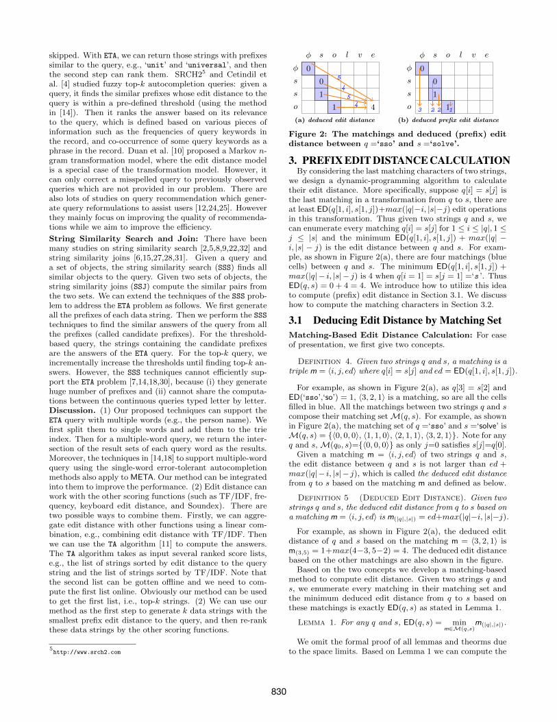
Figure 2: The matchings and deduced (prefix) editdistance between q =‘sso’ and s =‘solve’.
3. PREFIX EDIT DISTANCE CALCULATIONBy considering the last matching characters of two strings,
we design a dynamic-programming algorithm to calculatetheir edit distance. More specifically, suppose q[i] = s[j] isthe last matching in a transformation from q to s, there areat least ED(q[1, i], s[1, j])+max(|q|−i, |s|−j) edit operationsin this transformation. Thus given two strings q and s, wecan enumerate every matching q[i] = s[j] for 1 ≤ i ≤ |q|, 1 ≤j ≤ |s| and the minimum ED(q[1, i], s[1, j]) + max(|q| −i, |s| − j) is the edit distance between q and s. For exam-ple, as shown in Figure 2(a), there are four matchings (bluecells) between q and s. The minimum ED(q[1, i], s[1, j]) +max(|q|− i, |s|− j) is 4 when q[i = 1] = s[j = 1] =‘s ’. ThusED(q, s) = 0 + 4 = 4. We introduce how to utilize this ideato compute (prefix) edit distance in Section 3.1. We discusshow to compute the matching characters in Section 3.2.
3.1 Deducing Edit Distance by Matching SetMatching-Based Edit Distance Calculation: For easeof presentation, we first give two concepts.
Definition 4. Given two strings q and s, a matching is atriple m = 〈i, j, ed〉 where q[i] = s[j] and ed = ED(q[1, i], s[1, j]).
For example, as shown in Figure 2(a), as q[3] = s[2] andED(‘sso’,‘so’) = 1, 〈3, 2, 1〉 is a matching, so are all the cellsfilled in blue. All the matchings between two strings q and scompose their matching setM(q, s). For example, as shownin Figure 2(a), the matching set of q =‘sso’ and s =‘solve’ isM(q, s) = {〈0, 0, 0〉, 〈1, 1, 0〉, 〈2, 1, 1〉, 〈3, 2, 1〉}. Note for anyq and s,M(q0, s)={〈0, 0, 0〉} as only j=0 satisfies s[j]=q[0].
Given a matching m = 〈i, j, ed〉 of two strings q and s,the edit distance between q and s is not larger than ed +max(|q|− i, |s|− j), which is called the deduced edit distancefrom q to s based on the matching m and defined as below.
Definition 5 (Deduced Edit Distance). Given twostrings q and s, the deduced edit distance from q to s based ona matching m = 〈i, j, ed〉 is m(|q|,|s|) = ed+max(|q|−i, |s|−j).
For example, as shown in Figure 2(a), the deduced editdistance of q and s based on the matching m = 〈3, 2, 1〉 ism(3,5) = 1+max(4−3, 5−2) = 4. The deduced edit distancebased on the other matchings are also shown in the figure.
Based on the two concepts we develop a matching-basedmethod to compute edit distance. Given two strings q ands, we enumerate every matching in their matching set andthe minimum deduced edit distance from q to s based onthese matchings is exactly ED(q, s) as stated in Lemma 1.
Lemma 1. For any q and s, ED(q, s) = minm∈M(q,s)
m(|q|,|s|).
We omit the formal proof of all lemmas and theorms dueto the space limits. Based on Lemma 1 we can compute the
(i−1,j−1)〉 in H 〈1, 0〉 〈1, 1〉 〈2, 2〉 〈2, 1〉 〈2, 1〉
edit distance based on the matching set. We show how tocalculate the matching set M(q, s) later in Section 3.2.
Matching-Based Prefix Edit Distance Calculation:The basic idea of the matching-based prefix edit distancecalculation is illustrated in Figure 2(b). Given a query q anda string s, to calculate their prefix edit distance PED(q, s)we need to find a transformation from q to a prefix of swith minimum number of edit operations. Suppose q[i] =s[j] is the last matching in this transformation, we havePED(q, s) = ED(q[1, i], s[1, j]) + (|q| − i), as the prefix editdistance is exactly the number of edit operations in thistransformation. Thus we can enumerate every matchingq[i] = s[j] between a query q and a string s and the mini-mum of ED(q[1, i], s[1, j])+(|q|−i) is the prefix edit distancebetween q and s. For example, as shown in Figure 2(b), theminimum of ED(q[1, i], s[1, j])+(|q|− i) is 1 when q[i = 3] =s[j = 2] =‘o ’ and thus PED(q, s) = 1 + 0 = 1. Next we givea concept and formalize our idea.
Definition 6 (Deduced Prefix Edit Distance).Forany two strings q and s, the deduced prefix edit distance fromq to s based a matching m = 〈i, j, ed〉 is m|q| = ed+ (|q|− i).
For example, as shown in Figure 2(b), the deduced prefixedit distance between q and s based on their matching m =〈3, 2, 1〉 is m3 = 1 + (3 − 3) = 1. The deduced prefix editdistance based on the other matchings are also shown in thefigure. Based on this definition we propose a matching-basedmethod to compute prefix edit distance. Given two stringsq and s we enumerate every matching in their matchingset and the minimum deduced prefix edit distance based onthese matchings is exactly PED(q, s) as stated in Lemma 2.
Lemma 2. For any q and s, PED(q, s) = minm∈M(q,s)
m|q|.
Based on Lemma 2, we can compute the prefix edit dis-tance based on the matching set. Next we discuss how tocalculate the matching set M(q, s).
3.2 Calculating the Matching SetAs M(qi−1, s) ⊆ M(qi, s), we can calculate M(qi, s) in
an incremental way, i.e., calculate the matchings 〈i, j, ed〉in M(qi, s)−M(qi−1, s) for each 1 ≤ i ≤ |q|. More specifi-cally, we first initializeM(q0, s) as {〈0, 0, 0〉}. Then for each1 ≤ i ≤ |q|, we find all the 1 ≤ j ≤ |s| s.t. s[j] = q[i] and cal-culate ed = ED(q[1, i], s[1, j]) using M(qi−1, s). We have anobservation that if q[i] = s[j], ED(q[1, i], s[1, j]) is exactly theminimum of m(i−1,j−1) where m ∈M(qi−1, s[1, j−1]). Thisis because on the one hand, Ukkonen [26] proved when q[i] =s[j], ED(q[1, i], s[1, j]) = ED(q[1, i−1], s[1, j−1]) and on theother hand, based on Lemma 1, ED(q[1, i− 1], s[1, j − 1]) isthe minimum of m(i−1,j−1) where m ∈ M(qi−1, s[1, j − 1]).Thus ED(q[1, i], s[1, j]) = minm∈M(qi−1,s[1,j−1]) m(i−1,j−1) asstated in Lemma 3.
Lemma 3. Given two strings q and s, for any q[i] = s[j]we have ED(q[1, i], s[1, j]) = min
m∈M(qi−1,s[1,j−1])m(i−1,j−1).
In addition, asM(qi−1, s[1, j−1]) is a subset ofM(qi−1, s),we can enumerate every m′ = 〈i′, j′, ed′〉 in M(qi−1, s) s.t.j′ < j
(which indicates m′ ∈ M(qi−1, s[1, j − 1])
)and the
Algorithm 1: MatchingSetCalculation
Input: q: a query string; s: a data string.Output: M(q, s): the matching set of q and s.M(q0, s) = {〈0, 0, 0〉};1
foreach qi where 1 ≤ i ≤ |q| do2
H = φ; // minimum deduced edit distance3
foreach m′ = 〈i′, j′, ed′〉 ∈ M(qi−1, s) do4
foreach j > j′ s.t. q[i] = s[j] do5
if H[j] > m′(i−1,j−1) then H[j] = m′(i−1,j−1)6
foreach entry 〈j, ed〉 in H do7
add the matching 〈i, j, ed〉 to M(qi, s);8
add all the matchings in M(qi−1, s) to M(qi, s);9
output M(q, s);10
minimum of m′(i−1,j−1) is exactly the minimum of m(i−1,j−1)
where m ∈ M(qi−1, s[1, j − 1]). In this way we can get edand the new matching 〈i, j, ed〉 inM(qi, s)−M(qi−1, s). Allthese new matchings and all those matchings in M(qi−1, s)forms M(qi, s). Finally we can get M(q, s).
The pseudo code of the matching set calculation is illus-trated in Algorithm 1. It takes two strings q and s as inputand outputs their matching set. It first initializes M(q0, s)as {〈0, 0, 0〉} (Line 1). Then for each 1 ≤ i ≤ |q|, it initial-izes a hash map H to keep the minimum deduced edit dis-tance (Lines 2 to 3). For each matching m′ = 〈i′, j′, ed′〉 ∈M(qi−1, s), it finds all j > j′ s.t. q[i] = s[j], calculatesthe deduced edit distance m′(i−1,j−1), and updates H[j] if
m′(i−1,j−1) is smaller (Lines 4 to 6). Then for each entry〈j, ed〉 in the hash map H, it adds the matching 〈i, j, ed〉 toM(qi, s). (Lines 7 to 8). In addition, it adds all the match-ings in M(qi−1, s) to M(qi, s) (Line 9). Finally it outputsthe matching set M(q, s) (Line 10).
Example 1. Table 2 shows a running example of the mat-ching set calculation. Note the entries in H with deletionsare replaced by others. We first set M(q0, s) = {〈0, 0, 0〉}.For i = 1, for the matching m′ = 〈0, 0, 0〉, we have j = 1s.t. q[1] = s[1]. Thus we set H[1] = m′(0,0) = 0. We tra-verse H and add 〈1, 1, 0〉 toM(q1, s). We also add 〈0, 0, 0〉 ∈M(q0, s) to M(q1, s). Thus M(q1, s) = {〈0, 0, 0〉, 〈1, 1, 0〉}.For i = 2, for m′ = 〈0, 0, 0〉 we have j = 1 s.t. q[2] = s[1].Thus we set H[1] = m′(1,0) = 1. For m′ = 〈1, j′ = 1, 0〉, as
q[2] 6= s[j] for any j > j′ = 1, we do nothing. We traverse Hand add 〈2, 1, 1〉 to M(q2, s). We also add the matchings inM(q1, s) to it and haveM(q2, s) = {〈0, 0, 0〉, 〈1, 1, 0〉, 〈2, 1, 1〉}.For i = 3, for m′ = 〈0, 0, 0〉, we set H[2] = m′(2,1) = 2. For
m′ = 〈1, 1, 0〉, as m′(2,1) = 1 < H[2] = 2, we update H[2] as 1.
For m′ = 〈2, 1, 1〉, as m′(2,1) = 1 is not smaller than H[2] =1, we do not update H[2]. We traverse H and add 〈3, 2, 1〉 toM(q3, s). We also add the matchings in M(q2, s) to it andhave M(q3, s) = {〈0, 0, 0〉, 〈1, 1, 0〉, 〈2, 1, 1〉, 〈3, 2, 1〉}. Notebased on Lemmas 1 and 2 we have ED(q3, s) = 〈1, 1, 0〉(3,5) =4 and PED(q3, s) = 〈3, 2, 1〉3 = 1.
4. THE MATCHING-BASED FRAMEWORKIn this section, we calculate the prefix edit distance be-
tween a query and a set of data strings. We first design amatching-based framework for threshold-based queries andthen extend it to support top-k queries in Section 6.
831
Table 3: A running example of the matching-based framework (τ = 2, q=‘sso’, T in Figure 1).i and query qi i = 1, q1 = s i = 2, q2 = ss i = 3, q3 = sso
Indexing. We index all the data strings into a trie. Wetraverse the trie in pre-order and assign each node an idstarting from 1. For each leaf node, we also assign it withthe corresponding string id. For example, Figure 1 showsthe trie index for the dataset S in Table 1. Each node n inT contains a label n.char, an id n.id, a depth n.depth = |n|and a range n.range = [n.lo, n.up] where n.lo and n.up arerespectively the smallest and largest node id in the subtreerooted at n. Each node n corresponds to a prefix whichis composed of the characters from the root to n. All thestrings in the subtree rooted at n share this common pre-fix. For simplicity, we interchangeably use node n with itscorresponding prefix. We also use n.parent to denote theparent node of n. For each keystroke x, to efficiently findthe node n where n.char = x, we build a two-dimensionalinverted indexes I for the trie nodes where the inverted listI[depth][x] contains all the nodes n in T s.t. |n| = depthand n.char = x. The nodes in the inverted list are sortedby their id for ease of binary search.
Querying. Since each trie node corresponds to a prefix,the definitions of the matching and deduced (prefix) editdistance can be intuitively extended to trie nodes and weuse them interchangeably. For example, consider the trie inFigure 1 and suppose q =‘ss’. m = 〈2, n2, 1〉 is a matchingas n2.char = q[2] =‘s’ and ED(q[1, 2], n2) = 1. The deducededit distance from q to n3 based on m is m(2,|n3|=2) = 1 +max(2−2, 2−1) = 2. The deduced prefix edit distance of qbased on m is m|q|=2 = 1 + (2− 2) = 1. Next, we introducea concept and give the basic idea of querying.
Definition 7 (Active Matching and Active Node).Given a query q and a threshold τ , m = 〈i, n, ed〉 is an activematching of q and n is an active node of q iff m|q| ≤ τ .
Consider the example above and suppose τ = 2, we havem = 〈2, n2, 1〉 is an active matching of q and n2 is an activenode of q as m|q| = 1 ≤ τ . All the active matchings be-tween a query q and a trie T compose their active matchingsetA(q, T ). Following the example above we haveA(q, T ) ={〈0, n1, 0〉〈1, n2, 0〉〈2, n2, 1〉}. NoteA(q0, T )={〈0, T .root, 0〉}.
Next we give the basic idea of our matching-based frame-work. We have an observation that given a query q and athreshold τ , for any string s ∈ S, if PED(q, s) ≤ τ theremust exist an active matching 〈i, n, ed〉 of q s.t. s is a leafdescendant of n. This is because if PED(q, s) ≤ τ , based onLemma 2 there exists a matching m = 〈i, j, ed〉 ∈ M(q, s)s.t. m|q| = ed+(|q|−i) ≤ τ . Suppose n is the correspondingtrie node of the prefix s[1, j], we have q[i] = s[j] = n.charand ed = ED(q[1, i], s[1, j]) = ED(q[1, i], n). Based on Defi-nition 7, 〈i, n, ed〉 is an active matching of q as 〈i, n, ed〉|q| =ed+ (|q| − i) ≤ τ . Thus to answer a query, we only need tofind its active matching set. Next we show how to incremen-tally get A(qi, T ) based on A(qi−1, T ) for each 1 ≤ i ≤ |q|.
For each query qi, there are two kinds of active match-ings m′′ = 〈i′′, n′′, ed′′〉 in A(qi, T ). Those with i′′ < i andthose with i′′ = i. Note based on Definition 7, m′′i ≤ τ .For the first kind, m′′ is also an active matching of qi−1 asm′′i−1 = m′′i −1 ≤ τ−1 ≤ τ . Thus we can get all the first kindof active matchings from A(qi−1, T ). For the second kind,we have m′′i = ed′′ + (i− i′′) = ed′′ ≤ τ . To get all this kindof active matchings, we need to find all the nodes n′′ s.t.
Algorithm 2: MatchingBasedFramework
Input: T : a trie; τ : a threshold; q: a continuous query;Output: Ri={s ∈ S
∣∣PED(qi, s) ≤ τ} for each 1≤i≤|q|;A(q0, T ) = {〈0, T .root, 0〉};1
n′′.char = q[i] and ED(qi, n′′) ≤ τ , and calculate the value
ed′′ = ED(qi, n′′). Based on Lemma 3, for any node n′′ s.t.
n′′.char = q[i], ED(qi, n′′) is the minimum of m(i−1,|n′′|−1)
where m ∈ M(qi−1, n′′.parent). To satisfy ED(qi, n
′′) ≤ τ ,we require m(i−1,|n′′|−1) ≤ τ . As mi−1 ≤ m(i−1,|n′′|−1) ≤ τ ,m is an active matching of qi−1, i.e., m ∈ A(qi−1, T ). Thusfor each n′′ s.t. q[i] = n′′.char, we can enumerate ev-ery m′ = 〈i′, n′, ed′〉 ∈ A(qi−1, T ) where n′ is an ances-tor of n′′
(which indicates m′ ∈ M(qi−1, n
′′.parent))
andm′(i−1,|n′′|−1) ≤ τ , and the minimum of m′(i−1,|n′′|−1) is ex-
actly ed′′ = ED(qi, n′′) if ED(qi, n
′′) ≤ τ . In this way we canget ed′′ and all the second kind of active matchings.
The pseudo-code of the matching-based framework is shownin Algorithm 2. It takes a trie T , a threshold τ and a querystring q as input and outputs the result set Ri for eachquery qi where 1 ≤ i ≤ |q|. It first initializes A(q0, T )as {〈0, T .root, 0〉} (Line 1). Then for each query qi, itfirst initializes a hash map H = φ to keep the minimumdeduced edit distance (Line 3). Then, for each matchingm′ = 〈i′, n′, ed′〉 ∈ A(qi−1, T ), it finds all the descendantnodes n of n′ s.t. n.char = q[i] and m′(i−1,|n|−1) ≤ τ
and uses the deduced edit distances m′(i−1,|n|−1) to updateH[n] (Line 4 to 7). Next for each entry 〈n, ed〉 in H, itadds the active matching 〈i, n, ed〉, which is the second kindas described above, to A(qi, T ) (Lines 8 to 9). For eachm′ ∈ A(qi−1, T ), if m′i ≤ τ , it adds the active matching m′,which is the first kind, to A(qi, T ) (Lines 10 to 11). Finally,it adds the leaves of the active nodes of the active matchingsin A(qi, T ) to Ri and outputs Ri (Lines 12 to 14).
Example 2. Table 3 shows a running example of the mat-ching based framework. For i = 3 and q3 =‘sso’, initially wehave A(q2, T ) = {〈0, n1, 0〉, 〈2, n2, 1〉, 〈1, n2, 0〉}. For m′ =〈0, n1, 0〉, we have the descendants n3 and n12 of n1 s.t.q[3] = n3.char and q[3] = n12.char and m′(3−1,|n3|−1) = 2 ≤τ and m′(3−1,|n12|−1) = 2 ≤ τ . Thus we set H[n3] = 2 and
H[n12] = 2. For m′ = 〈2, n2, 1〉, the descendants n3 and n12
of n2 have the same label as q[3] and m′(2,1) = 1 < H[n3]
and m′(2,2) = 2 ≥ H[n12]. Thus we only update H[n3] = 1.
832
Note the descendants n5 and n11 of n2 also have the samelabel as q[3]. However we skip them as m′(2,3) = 3 > τ .
For m′ = 〈1, n2, 0〉, the descendants n3, n12, n5 and n11 ofn2 have the same label as q[3] and m′(2,1) = 1, m′(2,2) = 1,
m′(2,3) = 2 and m′(2,3) = 2. Thus we update H[n12] = 1and set H[n5] = 2 and H[n11] = 2. Then we traverse H andadd 〈3, n3, 1〉, 〈3, n12, 1〉,〈3, n5, 2〉 and 〈3, n11, 2〉 to A(q3, T ).Next we traverse A(q2, T ) and add 〈2, n2, 1〉 and 〈1, n2, 0〉 toA(q3, T ). Note we do not add m′ = 〈0, n1, 0〉 as m′3 = 3 > τ .Finally we add the strings on the leaf descendants of n2, n3,n5, n11 and n12 to R3 and output R3 = {s1, s2, s3, s4, s5}.
Note in the matching-based framework, for each m′ =〈i′, n′, ed′〉 ∈ A(qi−1, T ) we need to find all the descendantsn of n′ s.t. n.char = q[i] and m′(i−1,|n|−1) ≤ τ . We can
achieve this by binary searching I[d][q[i]
]where d ∈ [|n′|+
1, |n′| + τ + 1] to get nodes n with id within n′.range andm′(i−1,|n|−1) ≤ τ . This is because on the one hand these
nodes have label same as q[i] and are descendants of n′. Onthe other hand for any descendant n of n′, m′(i−1,|n|−1) =
The matching-based framework satisfies correctness andcompleteness as stated in Theorem 1.
Theorem 1. The matching-based framework satisfies (1)correctness: for each string s found by the matching-basedframework, PED(q, s) ≤ τ , and (2) completeness: for eachstring s ∈ S satisfying PED(q, s) ≤ τ , it must be reported bythe matching-based framework.
Complexity: The time complexity for answering query qiis O
(|A(qi−1, T )|τ log |S| + |A(qi, T )|(τ2 + log |S|)
)where
binary searching inverted lists costs O(|A(qi−1, T )|τ log |S|),getting matching set costs O(|A(qi, T )|τ2) and getting theresults costs O(|A(qi, T )| log |S|) as we can store the datain the order of their ids and perform binary search for eachactive matching to get the results. The space complexity isO(|S|) as S is larger than T , H and the matching sets.
5. COMPACT TREE BASED METHODWe have an observation that the matching-based frame-
work has a large number of redundant computations. Con-sider two active matchings with the active nodes n and pas shown in Figure 3. If n = p, it leads to redundant com-putation on the descendants of n. We combine the activematchings with the same active node to avoid this type ofredundant computations in Section 5.1. If p is an ancestorof n, it may lead to redundant computation on the overlapregion of their descendants. We only check those descen-dants of n with depth in [|p|+ τ + 2, |n|+ τ + 1] to eliminatethis kind of redundant computations in Section 5.2. To ef-ficiently identify the active nodes with ancestor-descendantrelationship (such as p and n), we design a compact treeindex in Section 5.3. Lastly, we discuss how to maintain thecompact tree index in Section 5.4.
5.1 Combining Active MatchingsWe have an observation that some active matchings may
share the same active node n and we need to perform redun-dant binary searches on the descendants of n with depth in[|n| + 1, |n| + τ + 1]. For example, consider the two activematchings 〈1, n2, 0〉 and 〈2, n2, 1〉 of q2 in Example 2, weneed to check the descendants of n2 twice. To address this
p
n
n p
n
d
d d
(a) active matchings with
the same active node (b) active nodes with nearest ancestor relationship
issue, we combine the active matchings with the same ac-tive node. We use a hash map F to store all the activenodes where F [n] contains all the active matchings withthe active node n. For each query qi, for each node n s.t.n.char = q[i], the matching-based framework enumeratesevery m ∈ A(qi−1, T ) and uses m(i−1,|n|−1) to update H[n].To achieve the same goal with F , we enumerate every ac-tive node n′ ∈ F and use minm∈F[n′] m(i−1,|n|−1) to updateH[n]. We discuss more details of utilizing F to answer thethreshold-based query in Section 5.3.
5.2 Avoiding Redundant Binary SearchBoth the matching-based framework and all the previous
works [7,14,18,30] store the active nodes in a hash map andprocess them independently, and they involve many redun-dant computations. Using the matching-based framework asan example, consider the two active matchings 〈0, n1, 0〉 and〈1, n2, 0〉 of q2 in Example 2, as [|n1|+1, |n1|+τ +1] = [1, 3]and [|n2| + 1, |n2| + τ + 1] = [2, 4], it needs to perform du-plicate binary searches on both I
[2][q[3]
]and I
[3][q[3]
].
Next we formally discuss how to avoid the redundant com-putations. Consider two active nodes n and p of the queryqi−1 where p is an ancestor of n as shown in Figure 3(b).In the matching-based framework, we need to perfom bi-nary search on the inverted lists I
[d][q[i]
]to find nodes
with id within n.range where d ∈ [|n| + 1, |n| + 1 + τ ] andon the inverted lists I
[d′][q[i]
]to find nodes with id within
p.range where d′ ∈ [|p| + 1, |p| + 1 + τ ]. As p.range cov-ers n.range, the binary search on the overlap region forn.range is redundant. To avoid this, for the active noden, we do not perform binary searches on the overlap region,i.e., we only perform the binary search on I
[d][q[i]
]where
d ∈ [max(|n|+ 1, |p|+ 2 + τ), |n|+ 1 + τ ] to get nodes withid within n.range. Thus we can eliminate all the redun-dant binary search by maintaining the ancestor-descendantrelationship between the active nodes. As |p| + 2 + τ ismonotonically increasing with the depth |p| and the nearestancestor of n has the largest depth, we only need the nearestancestor p of n to avoid the redundant binary searches. Tothis end, we design a compact tree index to keep the nearestancestor relationship for the active nodes in Section 5.3.
5.3 The Compact Tree based MethodTo effectively maintain the nearest ancestor for each active
node, we design a compact tree index for the active nodes.
Definition 8 (Compact Tree). The compact tree ofa query is a tree structure, which satisfies,(1) There is a bijection between the compact nodes and theactive nodes of the query.(2) For any two compact nodes p and n and their corre-sponding active nodes p′ and n′, p is the parent of n iff p′ isthe nearest ancestor of n′ among all the active nodes.
833
Table 4: A running example of the compact tree based method (τ = 2, q=‘ssol’, T in Figure 1).i and query qi i = 1, q1 = s i = 2, q2 = ss i = 3, q3 = sso i = 4, q4 = ssol
n ∈ F (n ∈ C) n1 n1 n2 n1 n2 n2 n3 · · ·m ∈ F [n] 〈0, n1, 0〉 〈0, n1, 0〉 〈1, n2, 0〉 〈0, n1, 0〉
Input: T : a trie; τ : a threshold; q: a continuous query;Output: Ri = {s ∈ S
∣∣PED(qi, s)≤τ} for each 1≤i≤|q|;F [T .root] = {〈0, T .root, 0〉} and add T .root to C;1
foreach query qi where 1 ≤ i ≤ |q| do2
traverse C in pre-order and get all its nodes;3
foreach compact node n in pre-order do4
foreach d ∈ [max(|n|+ 1, |p|+ 2 + τ),5
|n|+ 1 + τ ] where p is the parent of n in C doL = BinarySearch(I
[d][q[i]
], n.range);6
h = minm∈F[n]m(i−1,d−1);7
AddIntoCompactTree(n,L, d, i, h);8
foreach compact node n in C do9
foreach m ∈ F [n] do remove m if mi > τ ;10
if F [n] = φ then11
remove n from F , and C by setting the12
parent of n as the parent of n’s children;
foreach first-level compact node n in C do13
add all the leaf descendants of n to Ri;14
output Ri;15
(3) The children of a compact node are ordered by their ids.
For example, Figure 5 shows the compact tree of the queryq3 in Example 2. Note the active nodes of q3 are shown inFigure 1 with bold border. For ease of presentation, we in-terchangeably use the compact node with its correspondingactive node when the context is clear.
We discuss how to build and maintain the compact tree inSection 5.4. In this section we focus on utilizing the compacttree to answer the threshold-based query while avoiding theredundant binary search. The compact tree based methodis similar to the matching-based framework except that theactive nodes are processed in a top-down manner, we onlybinary search the non-overlapping region of the descendantsof an active node and the active-node set F and the compacttree C are updated in-place. The pseudo code is shown in Al-gorithm 3. Initially, it sets F [T .root] = {〈0, T .root, 0〉} andinserts the active node T .root of q0 to the empty compacttree C (Line 1). Then for each query qi, instead of process-ing the active nodes independently, it processes them in atop-down manner. Specifically, it first traverses the compacttree in pre-order and gets all the compact nodes (Line 3).Then for each compact node n (in pre-order), for each depthd ∈ [max(|n|+1, |p|+2+τ), |n|+1+τ ] where p is the parentof n in the compact tree, it binary searches the inverted listI[d][q[i]
]to get a list L of ordered nodes with id within
n.range, i.e., the nodes in L are ordered, have label q[i],with depth d and are descendants of n (Lines 4 to 6). Thenit inserts the active nodes in L to the compact tree C andadds the corresponding active matchings, which are the sec-ond kind as described in Section 4, to F using the procedureAddIntoCompactTree which we discuss later in Section 5.4.Note h is used to keep the minimum deduced edit distance(Lines 7 to 8). Next for each compact node n, it removesthe non-active matchings m in F [n] where mi > τ and thusall the first kind of active matchings are remained in F [n]
(Line 10). If all the matchings in F [n] are removed, it alsoremoves the node n from F and C by pointing the parent ofn to the children of n (Line 12). Finally it adds all the leafdescendants of the first-level compact nodes in C to Ri andoutputs Ri as the leaf descendants of all the other compactnodes are covered by those of the first-level (Lines 14 to 15).
Example 3. Table 4 shows a running example of the com-pact tree based method. For query q3, we traverse C and gettwo compact nodes n1 and n2. For n1, as [max(0+1,−∞+2 + 2), 0 + 1 + 2] = [1, 3] (Note if a compact node has noparent p in C, we set |p| as −∞), we binary search I[1][o],I[2][o], and I[3][o] for n1.range and get three lists L of or-dered nodes φ, {n3} and {n12}. For the compact node n2, as[max(1+1, 0+2+2), 1+1+2] = [4, 4], we binary search theinverted list I[4][o] for n2.range and get a list L of orderednodes L = {n5, n11}. Note we only show the non-empty listsin the table. We discuss later how to add the active nodes inthese lists to C and F . For node n1, as 〈0, n1, 0〉3 = 3 > τ ,we remove it from F [n1] and have F [n1] = φ. Thus we alsoremove n1 from F and C and now C is that in Figure 5.Finally we add the leaves of the first-level compact node n2
in C to R3 and have R3 = {s1, s2, s3, s4, s5}.We can see that for each query, each trie node is accessed
at most once by the active nodes. The compact tree basedmethod is correct and complete as stated in Theorem 2.
Theorem 2. The compact tree based method satisfies cor-rectness and completeness.
5.4 Adding Active Nodes to the Compact TreeFor a query qi, for a compact node n and a depth d, the
compact tree based method binary searches the inverted listI[d][q[i]
]and get a list L of ordered nodes which are all
descendants of n in the trie and with depth d. In this sectionwe focus on inserting the active nodes in L to the compacttree and add the corresponding active matchings to F . Thebasic idea is that for each node a ∈ L we find a properposition for it in C. Then we compute ed = ED(qi, a) ifED(qi, a) ≤ τ . As ed+ (i− i) = ed ≤ τ , 〈i, a, ed〉 is an activematching and we add it to F [a]. In addition, a is an activenode and we insert a to C at the proper position.
We first discuss how to find a proper position in C for anode a ∈ L to insert to. The proper position for a in Cshould satisfy the three conditions in Definition 8. As thenode a ∈ L is a descendant of n in the trie, based on condi-tion 2 of Definition 8, we should also insert a as a descendantof n in the compact tree. Based on condition 3 of Defini-tion 8, the children of n are already ordered and the properposition for a in C should keep the children of n ordered.To this end, we develop a procedure AddIntoCompactTree
which sequentially compare a with each child c of n and tryto find the proper position for a as a child of n. There arefive cases in the comparison of a and c as shown in Figure 4.Case 1: a is on the left of c, i.e., a.up < c.lo. In this casethe proper position of a is exactly the left of c and the childof n as the comparisons are performed sequentially and theleft siblings of c are all smaller than a.Case 2: a is an ancestor of c, i.e., c.range ⊂ a.range. Inthis case, based on condition 2 of Definition 8, the proper
834
�
������
������ ������
�����
�� ������������
�������������
��������������
� �
�
�
�
�
�
�
�
�
�
�������
�
�
�
� �
�
������
�
���������� �� �
�
� �
�
�
�
�
��������� �������
�����
��
����������������������� �����
Figure 4: Comparing nodes in L with children of the compact node n.
position of a is the child of n and the parent of c and all theright siblings c′ of c s.t. c′.range ⊂ a.range.Case 3: a = c, i.e., a.range = c.range. In this case aalready exists in the compact tree. To satisfy the condition1 of Definition 8, we do not insert a to C. Thus there is noproper position for a in the compact tree.Case 4: a is a descendant of c, i.e., a.range ⊂ c.range. Inthis case, based on condition 2 of Definition 8, the properposition of a in C should be a descendant of c. Thus werecursively invoke the procedure AddIntoCompactTree whichcompares a with the children of c to find the proper position.Case 5: a is on the right of c, i.e., c.up < a.lo. In this case,to keep the descendants of n ordered, we skip c and comparea with the next sibling of c.
Note if c reaches the end, a is larger than all the childrenof n and the proper position for a is the last child of n.Based on the structure of trie and compact tree, all the othercases cannot happen. Thus we can recursively find a properposition in C for each node in L. Moreover, as the nodes in Lare ordered and so are the children of n, instead of processingeach node in L independently, we actually can perform thecomparison between all the nodes in L and all the childrenof n in a merging fashion. Specifically, we first compare thefirst node in L with the first child of n. Whenever we getthe proper position in C for a node a ∈ L, we continuouslycompare the next node of a in L with the current child c ofn and check the five cases until we reach the end of L. Inthis way we can get all the proper positions for nodes in L.
Next we discuss how to compute ed = ED(qi, a) in the sit-uation ED(qi, a) ≤ τ where a ∈ L and |a| = d. Based on thediscussion in Section 4, when ED(qi, a) ≤ τ , ED(qi, a) is theminimum of m(i−1,|a|−1) , where m = 〈i′, n′, ed′〉 is an activematching of qi−1 inM(qi−1, a.parent) s.t. m(i−1,|a|−1) ≤ τ .As m is an active matching, n′ is an active node and n′
is in C. Moreover, as m ∈ M(qi−1, a.parent), n′ is an
ancestor of a in the trie. Based on condition 2 of Defini-tion 8, n′ is also an ancestor of a in C. In addition, asτ ≥ m(i−1,|a|−1) = ed′ + max(i − 1 − i′, d − 1 − |n′|) ≥d − 1 − |n′| ≥ |p| + 2 + τ − 1 − |n′| where p is the nearestancestor of n among all active nodes, we have |n′| > |p|.Thus n′ is on the path from n (included) to a (not in-cluded) in C. Thus to get ED(qi, a) we only need to enu-merate every active node n′ on the path from n to a andthe minimum of minm∈F[n′] m(i−1,d−1) is ed = ED(qi, a) if
ED(qi, a) ≤ τ . We can achieve this simultaneously with theprocessing of finding the proper position for a by updating has minm∈F[c] m(i−1,d−1) if the latter is smaller whenever weinvoke the procedure AddIntoCompactTree in Case 4. Fi-nally if ed ≤ τ , 〈i, a, ed〉 is an active matching and we addit to F [a]. In addition, a is an active node and we insert ato the proper position in C.
Example 4. Figure 5 gives an example of adding a nodeto the compact tree C of the query q3 =‘sso’. For i = 4and q4 =‘ssol’, for node n2 and d = 3, we have L = {n6}.Next we add n6 to C and calculate ED(q4, n6). We use hto keep the minimum deduced edit distance. As F [n2] ={〈1, n2, 0〉, 〈2, n2, 1〉}, initially we set h = 〈1, n2, 0〉(3,2) = 2.We first compare n6 with the first child n3 of n2 and wehave n3.range ⊂ n6.range (Case 4). Thus we recursivelyinvoke this procedure and update h as 〈3, n3, 1〉(3,2) = 1 asF [n3] = {〈3, n3, 1〉}. We compare n6 with the first child n5
of n3 and have n5.u < n6.l (Case 5). Thus we move forwardand compare n6 with next sibling n11 of n5. As n11.range ⊂n6.range (Case 2) and n12.range 6⊂ n6.range, the properposition for n6 in C is the child of n3 and the parent of n11.Moreover as h = 1 ≤ τ , we add the active matching 〈4, n6, 1〉to F [n6] and insert n6 to the proper position in C.
Complexity: The time complexity for answering query qi isO(|C|τ log |S|+ |A(qi, T )|τ2 + |C′| log |S|) where C and C′ arerespectively the compact trees before and after processingthe query qi. Note |C| ≤ |A(qi−1, T )| and |C′| ≤ |A(qi, T )|.Also in practice we can skip the redundant binary searchesand the cost for binary search is smaller than O(|C|τ log |S|).The space complexity is O(|S|).
6. SUPPORTING TOP-K QUERIESGiven two continuous queries qi and qi+1, suppose bi+1 (or
bi) is the maximum prefix edit distance between qi+1 (or qi)and its top-k results. We prove that bi+1 = bi or bi+1 = bi+1(Section 6.1). Thus we can first use the same techniques forthreshold-based queries to find all strings with prefix editdistance to qi+1 equal to bi. If there are not enough results,we expand the matching set and find those data strings withprefix edit distance to qi+1 equal to bi + 1 until we get kresults (Section 6.2). In this way, we can answer the top-kquery using the matching-based method (Section 6.3).
6.1 The b-Matching SetGiven two queries qi−1 and qi, where qi is a new query
by adding a keystroke after qi−1, and let Ri denote thetop-k answers of qi and bi denote the maximal prefix editdistance between qi and the top-k answers of qi (i.e., bi =maxs∈Ri PED(qi, s)). We have an observation that eitherbi = bi−1 or bi = bi−1 + 1. This is because on the one hand,for any s ∈ Ri−1, we have PED(qi, s) ≤ PED(qi−1, s) + 1 ≤bi−1+1 as we can first delete the last character of qi and thentransform the rest of qi to a prefix of s with PED(qi−1, s)edit operations. Thus there are at least k strings in S with
835
prefix edit distances to qi no larger than bi−1 + 1 whichleads to bi ≤ bi−1 + 1. On the other hand, for any strings, based on the definition of prefix edit distance, we havePED(qi, s) ≥ PED(qi−1, s), i.e., the prefix edit distance fromthe continuous query to a string is monotonically increasingwith the query length. This leads to bi ≥ bi−1. Thus wehave either bi = bi−1 or bi = bi−1 + 1 as stated in Lemma 4.
Lemma 4. Given a continuous top-k query q, for any 1 ≤i ≤ |q| we have either bi = bi−1 or bi = bi−1 + 1.
For example, consider the dataset in Table 1. For the top-3 queries q1=‘s’, q2=‘ss’, and q3=‘sso’, we have b1 = 0, b2 = 1and b3 = 1. Note b0 = 0 for any top-k query q.
Based on Lemma 4 we give the basic idea of the matching-based method for top-k query. For each query qi, as eitherbi = bi−1 or bi = bi−1 + 1, we first find all the strings in Swith prefix edit distance to qi less than bi−1. Then we findthose equal to bi−1 until we get k results and set bi = bi−1.If there are not enough results, we continuous to find thoseequal to bi−1 + 1 until we get k results and set bi = bi−1 + 1.In this way we can answer the top-k query. The challenge inthe matching-based method is how to get the strings withspecific prefix edit distance to a query. Before addressingthis challenge, we introduce a concept.
Definition 9 (b-matching). A matching 〈i, n, ed〉 is ab-matching iff ed ≤ b. It is an exact b-matching iff ed = b.
For example, the matching 〈1, n2, 0〉 of q2 =‘ss’ is a 1-matching. All the b-matchings of a query q compose its b-matching set P(q, b, T ), abbreviated as P(q, b) if the contextis clear. For example, P(q2, 1)={〈0, n1, 0〉,〈1, n2, 0〉,〈2, n2, 1〉}.
We have an observation that given a query q, for anystring s ∈ S, if PED(q, s) ≤ b, there must exist a b-matching〈i, n, ed〉 s.t. s is a leaf descendant of n. This is becausebased on Lemma 2, if PED(q, s) ≤ b, there exists a matchingm = 〈i, j, ed〉 s.t. m|q| = ed + (|q| − i) ≤ b. Suppose n isthe corresponding node of s[1, j] in the trie T , 〈i, n, ed〉 isa b-matching as ed = ED(q[1, i], s[1, j]) = ED(q[1, i], n) anded ≤ ed + (|q| − i) ≤ b. Thus we can use P(q, b) to get allthe strings in S with prefix edit distance to q within b.
Moreover, given a continuous query q, for any integer band 1 ≤ i ≤ |q|, we find that we can (1) calculate P(qi, b −1) based on P(qi−1, b) and (2) calculate P(qi, b) based onP(qi, b − 1). We discuss how to achieve these later in Sec-tion 6.2. Thus given a b-matching set P(qi−1, b), we cancalculate P(qi, b− 1), P(qi, b), and P(qi, b+ 1) as follows.
P(qi−1, b)(1)−−→ P(qi, b− 1)
(2)−−→ P(qi, b)(2)−−→ P(qi, b+ 1)
Then we can answer the top-k query using the b-matchingset as follows. Given a trie T and a continuous query q, ini-tially we have b0 = 0 and P(q0, 0) = {〈0, T .root, 0〉}. Thenfor each 1 ≤ i ≤ |q|, we can use P(qi−1, bi−1) to calculateP(qi, bi) and answer the query qi. This is because on the onehand, we can use P(qi−1, bi−1) to calculate P(qi, bi−1 − 1),P(qi, bi−1) and P(qi, bi−1 + 1). On the other hand, we canuse P(qi, bi−1 − 1), P(qi, bi−1) and P(qi, bi−1 + 1) to getall the strings with prefix edit distance to qi less than bi−1,equal to bi−1 and equal to bi−1 + 1. Based on Lemma 4,Ri can be achieved from these strings and P(qi, bi) is eitherP(qi, bi−1) or P(qi, bi−1 + 1). In this way we can answer thecontinuous query q. Next we calculate the b-matching sets.
6.2 Calculating the b-Matching SetWe first discuss calculating P(qi, b−1) based on P(qi−1, b),
which is (almost) all the same as the incremental activematching set calculation when τ = b−1 in Section 4. Thereare two kinds of (b−1)-matchings m′′=〈i′′, n′′, ed′′〉 in P(qi, b−1). Those with i′′ > i and those with i′′ = i. Based onDefinition 9, ed′′ ≤ b − 1. For the first case, m′′ is also ab-matching in P(qi−1, b) as ed′′ ≤ b−1 ≤ b. Thus we can getall of them from P(qi−1, b). To get all the (b−1)-matchingswhere i = i′′, for each node n′′ s.t. n′′.char = q[i], we enu-merate every m′ = 〈i′, n′, ed′〉 ∈ P(qi−1, b) where n′ is an an-cestor of n′′ and m′(i−1,|n′′|−1) ≤ b−1, and have the minimum
of m′(i−1,|n′′|−1) is ed′′=ED(qi, n′′) if ED(qi, n
′′) ≤ b−1. This
is because based on Lemma 3 ED(qi, n′′) is the minimum of
m′(i−1,|n′′|−1) where m′ = 〈i′, n′.ed′〉 ∈ M(qi−1, n′′.parent)
while m′ should also be a b-matching and thus in P(qi−1, b)as ed′ ≤ m′(i−1,|n|−1) ≤ b−1 ≤ b. In this way we can also getall the second kind of (b−1)-matchings based on P(qi−1, b).
Next we discuss calculating P(qi, b) based on P(qi, b− 1).As P(qi, b−1) ⊆ P(qi, b), we only need to calculate those ex-act b-matchings in P(qi, b)−P(qi, b−1). Consider any exactb-matching m′′ = 〈i′′, n′′, ed′′ = b〉 in P(qi, b)− P(qi, b− 1).Based on Lemma 3, as q[i′′] = n′′.char, there exists a match-ing m′ = 〈i′, n′, ed′〉 ∈ M(qi′′−1, n
′′.parent) s.t. ed′′ =m′(i′′−1,|n′′|−1). This leads to ed′ ≤ m′(i′′−1,|n′′|−1) = ed′′ =
b. If ed′ < b, m′ is a (b− 1)-matching in P(qi, b− 1). Other-wise, ed′ = b and m′ is an exact b-matching in P(qi, b) −P(qi, b − 1). Thus to get all the exact b-matchings, wecan enumerate every (b − 1)-matching m′ = 〈i′, n′, ed′〉 inP(qi, b−1) and find all the descendants n′′ of n′ and i′′ > i′
s.t. q[i′′] = n′′.char and m′(i′′−1,|n′′|−1) = b. If 〈i′′, n′′, ∗〉 6∈P(qi, b − 1) where ∗ denotes an arbitrary integer6, we haveED(qi′′ , n
′′) = b. This is because 〈i′′, n′′, ∗〉 6∈ P(qi, b − 1)indicates ED(qi′′ , n
′′) ≥ b while m′(i′′−1,|n′′|−1) = b indi-
cates ED(qi′′ , n′′) ≤ b. Thus 〈i′′, n′′, ed′′ = b〉 is an exact
b-matching. For the newly generated exact b-matchings, werepeat the process above until there is no more new exact b-matchings. In this way we can get all the exact b-matchingsin P(qi, b)−P(qi, b−1) and achieve P(qi, b) using P(qi, b−1).
6.3 Matching-based Method for Top-k QueriesBased on Lemma 4, it is easy to see that P(qi−1, bi−1) ⊆P(qi, bi) for any 1 ≤ i ≤ |q|. Thus we calculate the b-matching set in-place using P. The pseudo-code of thematching-based method for top-k queries is shown in Al-gorithm 4. It first initializes b0 = 0 and the 0-matching setP as {〈0, T .root, 0〉} (Line 1). Then for qi, it first gets allthe (bi−1 − 1)-matchings and adds them to P by the proce-dure FirstDeducing (Line 3). Then it gets all the stringswith prefix edit distance to qi less than bi−1 using P andadds them to Ri (Lines 4 to 5). Next it invokes the proce-dure SecondDeducing to get the rest of answers, sets bi andoutputs Ri (Lines 6 to 9). The procedure FirstDeducing isthe same as the inner loop of Algorithm 2. SecondDeducing
takes P, Ri, query length i, and two integers b and k asinput and outputs true if it finds enough results whose pre-fix edit distance to qi are b. For each m′ in P, if m′i = b,it adds the leaves of n′ to Ri until |Ri| = k and returnstrue (Lines 2 to 4). If there is not enough results, it findsall the descendants n′′ of n′ and i′′ > i′ s.t. q[i′′] = n′′.char
6We can achieve this by implementing P(qi, b) as a hash map and
use 〈i′, n′〉 as the key of the b-matching 〈i′, n′, ed′〉 in it.
836
Table 5: A Running Example of the Matching-based Method for Top-k Queries (k = 3, q=‘sso’, T in Figure 1).i, query qi and bi−1 i = 1, q1 = s, b0 = 0 i = 2, q2 = ss, b1 = 0 i = 3, q3 = sso, b2 = 1
Ri: the result set; b, k: two integers.Output: true if |Ri| = k. Otherwise, false.foreach m′ = 〈i′, n′, ed′〉 ∈ P do1
if m′i = b then2
add the leaves of n′ to Ri until |Ri| = k;3
if |Ri| = k then return true4
find all the descendants n′′ of n′ and i′′ > i′ s.t.5
q[i′′]=n′′.char and m′(i′′−1,|n′′|−1)=b and append
〈i′′, n′′, b〉 to P for looping if 〈i′′, n′′, ∗〉 6∈ P;
return false;6
and m′(i′′−1,|n′′|−1) = b and appends 〈i′′, n′′, b〉 to P to get
new exact b-matchings if 〈i′′, n′′, ∗〉 6∈ P (Line 5). Notethis can be achieved by binary searching I[|n′′|][q[i′′]], where|n′′| = |n′|+ 1 + b− ed′ and i′′ ∈ [i′ + 1, i′ + 1 + b− ed′] ori′′ = i′+1+b−ed′ and |n′′| ∈ [|n′|+1, |n′|+1+b−ed′] (lessthan 2b binary searches). Finally it returns false (Line 6).
Example 5. Table 5 shows a running example for top-kqueries. The last three rows show the achieved answers ormatchings with deduced (prefix) edit distance less than bi−1,equalling bi−1 and equalling bi−1 + 1 respectively. For thequery q3, we have b2 = 1. At first, P = {〈1, n2, 0〉, 〈0, n1, 0〉}.As the deduced (prefix) edit distances based on these match-ings are not less than b2 = 1, we do not find any results.Then we invoke SecondDeducing to find answers and match-ings with (prefix) edit distance equalling b2. For m = 〈1, n2, 0〉,as m3 = 2 6= b, we do not get any answers. However we havethe descendants n3 and n12 of n2 and i′′ = 3 > 1 s.t. thededuced edit distance based on m equal to b2 = 1. Thus weadd the two matchings 〈3, n3, 1〉 and 〈3, n12, 1〉 to P. Wethen process m = 〈3, n3, 1〉. As m3 = 1, we add the leaves ofn3 to R3 and get R3 = {s1, s2, s3}.
The matching-based method for top-k queries satisfiescorrectness as stated in Theorem 3.
Theorem 3. The matching-based method for top-k queriescorrectly finds the top-k results.
Complexity: For the top-k query qi, as FirstDeducing
is the same as the inner loop of Algorithm 2 by settingτ as bi−1 − 1, it costs O
Table 6: Datasets.Datasets Cardinality Avg Len Max Len Min Len |Σ|Word 146,033 8.77 30 1 27Querylog 1,000,000 19.06 32 2 56
O(|P(qi, bi)|bi log |S|) as for each matching in P(qi, bi) itconducts at most 2bi binary searches. Based on Definition 9,P(qi−1, bi−1) ⊆ P(qi, bi) and P(qi, bi−1 − 1) ⊆ P(qi, bi).Thus the overall time complexity isO
(|P(qi, bi)|(b2i+bi log |S|)
).
The space complexity is O(|S|).Discussion: When there are a lot of data strings with thesame maximum prefix edit distance to the query, we can re-rank them by the other scoring functions, such as TF/IDF.
7. EXPERIMENTSWe conducted extensive experiments to evaluate the effi-
ciency and scalability of our techniques. We compared ourmethod META with state-of-the-art approaches IncNGTrie [30],ICAN [14] and IPCAN [18]. As state-of-the-art methods can-not answer top-k queries, we extended them to support top-k queries as follows. Based on Lemma 4, for each queryqi, either bi=bi−1 or bi=bi−1+1. Thus we first invoked thestate-of-the-art methods to calculate all the strings with pre-fix edit distance to the query not larger than bi−1 basedon active node sets. If the number of returned strings isno smaller than k, we returned the smallest k results fromthem. Otherwise, we increased the threshold by 1 and in-voked the state-of-the-art methods with the new thresholdbi=bi−1+1 to calculate k results from scratch. We also com-pared with the string similarity search methods HSTree [27]and Pivotal [8] for threshold-based queries and HSTree [27]and TopK [9] for top-k queries using the adaptation as de-scribed in Section 2.2. We obtained all the source codesfrom the authors. All the methods were implemented us-ing C++ and compiled using g++ 4.8.2 with -O3 flag. Allthe experiments were conducted on a machine running on64-bit Ubuntu Server 12.04 LTS version with an Intel XeonE5-2650 2.00 GHz processor and 48 GB memory.Dataset: We used two real datasets Word and Query-log7. Word contained 146,033 English words. Querylogcontained 1 million query logs from AOL. The details aregiven in Table 6. We used 1000 common misspellings inWikipedia8 as queries for Word and randomly chose 1000strings from Querylog as the queries for Querylog. Wedid not make any change for queries and data on Query-log. These queries were representative as they containedtypos in real world. We reported the average querying timewhere τ and k were evenly distributed in [1,6] and [10,40].
7.1 Evaluating the Compact Tree based MethodIn this section we evaluated the compact tree. We im-
plemented two methods Matching and Compact. Matchingutilized the matching-based framework while Compact usedcompact tree to remove redundant computations. We firstvaried the threshold τ and fixed the query length of 4 and5 for Word and Querylog respectively. We reported theaverage number of binary searches used by the two methods
(d) AOL QueryLogFigure 6: Matching vs Compact: number of binary searches and avg. search time for threshold-based queries.
10-2
100
102
104
1 2 3 4
Ave
rag
e T
ime (
ms)
τ, query length=4
METAICAN
IPCAN
IncNGTriePivotal
HSTree
(a) English Word
10-2
100
102
104
106
1 2 3 4
Ave
rag
e T
ime (
ms)
τ, query length=5
METAICAN
IPCAN
PivotalHSTree
(b) AOL QueryLog
0
200
400
600
1 2 3 4
Ave
rag
e T
ime (
ms)
τ=4, query length
METAICAN
IPCAN
IncNGTriePivotal
HSTree
(c) English Word
0
1000
2000
1 2 3 4 5 6
Ave
rag
e T
ime (
ms)
τ=6, query length
METAICAN
IPCAN
(d) AOL QueryLogFigure 7: Comparing with state-of-the-arts for threshold-based queries: varying threshold and query length.
10-2
100
102
104
106
10 20 30 40
Ave
rag
e T
ime
(m
s)
k, query length=6
METAICAN
IPCAN
IncNGTrieTopK
HSTree
(a) English Word
100
102
104
106
10 20 30 40
Ave
rag
e T
ime
(m
s)
k, query length=10
METAICAN
IPCAN
TopKHSTree
(b) AOL QueryLog
10-2
100
102
104
106
1 2 3 4 5
Ave
rag
e T
ime
(m
s)
k=20, query length
METAICAN
IPCAN
IncNGTrieTopK
HSTree
(c) English Word
10-2
100
102
104
106
108
1 2 3 4 5 6 7 8
Ave
rag
e T
ime
(m
s)
k=40, query length
METAICAN
IPCAN
TopKHSTree
(d) AOL QueryLogFigure 8: Comparing with state-of-the-arts for top-k queries: varying k and query length.
on the two datasets. Figure 6(a) and 6(b) show the results.We can see that Compact only took about one sixth binarysearches of Matching. For example, on Querylog dataset,for τ=4, Matching took about 130,000 binary searches foreach query while Compact only took about 22,000 binarysearches. This is because the compact tree can avoid alarge number of redundant binary searches for the activematchings with same active node and for the active nodeswith ancestor-descendant relationships. We also comparedthe average search time for the two methods. Figure 6(c)and 6(d) show the results. We can see that Compact outper-formed Matching by 6 times. For example, on Querylog,for τ=4, the average time for Matching and Compact were150ms and 31ms respectively, because the search time de-pended on the number of binary searches (more than 80%)and Compact took fewer binary searches than Matching.
7.2 Comparison with State-of-the-art MethodsThreshold-Based Query. We compared META with ICAN[14], IPCAN [18], IncNGTrie [30], Pivotal [8] and HSTree [27]for threshold-based queries. We first varied the threshold τand fixed the query length of 4 and 5 for Word and Query-log respectively. We reported the average search time andFigure 7(a) and 7(b) show the results. Note IncNGTrie tookhuge memory to store the deletion neighborhoods and ac-tive nodes, and it ran out of memory on Querylog datasets.The similarity search methods Pivotal and HSTree could notfinish in reasonable time on Querylog dataset for largethresholds. META achieved the best performance and out-performed existing methods by an order of magnitude. Forexample, on Word dataset, for τ = 4, the average time forIncNGTrie, ICAN, IPCAN, META, Pivotal and HSTree wereabout 23ms, 78ms, 33ms, 5ms, 230ms and 548ms respec-tively. This is because our method META can save a lot of
redundant binary searches compared with the state-of-the-art approaches. The string similarity search methods wereslower as they had poor pruning power for extremely shortqueries and they generated huge number of prefixes. Noteon Querylog when τ = 1, the average result set size forquery prefixes with length 10 was around 87. It was 38 forquery prefixes with length 6 on Word when τ = 1.
We then varied the query length and fixed τ as 4 and 6 forWord and Querylog respectively. We reported the aver-age search time and Figure 7(c) and 7(d) show the results.META also achieved the best performance. For example,on Word dataset, for query length of 3, the average searchtime for IncNGTrie, ICAN, IPCAN, META, Pivotal and HSTreewere 22ms, 66ms, 31ms, 4ms, 188ms and 447ms respectively.
Top-k Query. We compared META with ICAN [14], IP-CAN [18], IncNGTrie [30], HSTree [27], and TopK [9] for top-k queries. We reported the average search time by varyingk and query length. Figure 8 shows the results. Note thatthe y-axles are log scale. We can see that META outper-formed the other methods by 1-4 orders of magnitudes. Forexample, as shown in Figure 8(c), on Word dataset, fork=20 and query length of 4, the average time for IncNGTrie,ICAN, IPCAN, META, HSTree and TopK were respectively22ms, 0.50ms, 0.10ms, 0.007ms, 250ms and 0.047ms. Thisis because META can answer the top-k query incrementally.IncNGTrie was slower than others as it took more time for ini-tialization. Our method outperformed the string similaritysearch methods as we shared the computations between thecontinuous queries typed in letter by letter while TopK andHSTree cannot. On Querylog when k=10, there were 34%and 5% of the query prefixes with lengths 10 and 8 whosemaximum prefix edit distance in their top-k results were nosmaller than 3; there were 58% and 18% when k = 40.
838
0
10
20
30
1 2 3 4
Ave
rag
e T
ime (
ms)
Scales (*30k), query length=3
META τ=3META τ=4
IPCAN τ=3IPCAN τ=4
(a) English Word
0
1000
2000
3000
1 2 3 4 5
Ave
rag
e T
ime (
ms)
Scales (*2m), query length=5
META τ=3META τ=4
IPCAN τ=3IPCAN τ=4
(b) AOL QueryLog
0
0.5
1
1.5
2
2.5
1 2 3 4
Ave
rag
e T
ime (
ms)
Scales (*30k), query length=6
META k=30META k=40
IPCAN k=30IPCAN k=40
(c) English Word
0
30
60
90
1 2 3 4 5
Ave
rag
e T
ime (
ms)
Scales (*1m), query length=10
META k=30META k=40
IPCAN k=30IPCAN k=40
(d) AOL QueryLog
Figure 9: Evaluating scalability for threshold-based queries and top-k queries.
7.3 ScalabilityWe evaluated the scalability of our method. We used the
same queries and varied the dataset sizes. Figure 9 shows theresults for both threshold-based queries and top-k queries.For threshold-based queries, we used a fixed query length of3 and 5 for Word and Querylog respectively and reportedthe average time for different thresholds. We can see thatMETA scaled very well on the two datasets. For example,on Word dataset, for τ = 4, the average time for 30,000strings, 60,000 strings, 90,000 strings and 120,000 stringswere respectively 1.1ms, 1.9ms, 2.6ms and 2.9ms. This is be-cause with the increase of dataset sizes, the size of the trieindex only slightly increased as many strings shared com-mon prefixes. We also evaluated the most efficient existingmethod IPCAN on the large dataset. IPCAN took more than1 second on the Querylog dataset with 4 million stringsfor τ = 4 and could not meet the high-performance require-ment. For top-k queries, we used a fixed query length of 6and 10 for Word and Querylog respectively, and reportedthe average time for different k’s. We can see that METAstill had good scalability for top-k queries. The average timeslightly decreased as with the increases of dataset sizes, themaximum prefix edit distance for the top-k queries decreasedwhile the number of active nodes slightly increased.
8. CONCLUSIONWe study the threshold-based and top-k error-tolerant
autocompletion problems. We propose a matching-basedframework. To the best of our knowledge, this is the firststudy on answering top-k queries. We design a compacttree index to effectively maintain the active nodes. We pro-pose an efficient method to incrementally answer the top-kqueries. Experimental results showed our method signifi-cantly outperformed state-of-the-art methods.
Acknowledgements. This work was partly supported by the 973
Program of China (2015CB358700), NSF of China (61272090, 61373024,
(Y1-L3)-FST13-GZ, 863 Program (2012AA012600), and Chinese Spe-
cial Project of Science & Technology(2013zx01039-002-002).
9. REFERENCES[1] A. V. Aho. Algorithms for finding patterns in strings. In
Handbook of Theoretical Computer Science, Volume A:Algorithms and Complexity (A), pages 255–300. 1990.
[2] A. Behm, S. Ji, C. Li, and J. Lu. Space-constrained gram-basedindexing for efficient approximate string search. In ICDE,pages 604–615, 2009.
[3] F. Cai, S. Liang, and M. de Rijke. Time-sensitive personalizedquery auto-completion. In CIKM, pages 1599–1608, 2014.
[4] I. Cetindil, J. Esmaelnezhad, T. Kim, and C. Li. Efficientinstant-fuzzy search with proximity ranking. In ICDE, pages328–339, 2014.
[5] S. Chaudhuri, K. Ganjam, V. Ganti, and R. Motwani. Robustand efficient fuzzy match for online data cleaning. In SIGMODConference, pages 313–324, 2003.
[6] S. Chaudhuri, V. Ganti, and R. Kaushik. A primitive operatorfor similarity joins in data cleaning. In ICDE, pages 5–16, 2006.
[7] S. Chaudhuri and R. Kaushik. Extending autocompletion totolerate errors. In SIGMOD Conference, pages 707–718, 2009.
[8] D. Deng, G. Li, and J. Feng. A pivotal prefix based filteringalgorithm for string similarity search. In SIGMOD Conference,pages 673–684, 2014.
[9] D. Deng, G. Li, J. Feng, and W.-S. Li. Top-k string similaritysearch with edit-distance constraints. In ICDE, pages 925–936,2013.
[10] H. Duan and B. P. Hsu. Online spelling correction for querycompletion. In WWW, pages 117–126, 2011.
[11] R. Fagin, A. Lotem, and M. Naor. Optimal aggregationalgorithms for middleware. In PODS, 2001.
[12] J. Guo, X. Cheng, G. Xu, and H. Shen. A structured approachto query recommendation with social annotation data. InCIKM, pages 619–628, 2010.
[13] S. Ji and C. Li. Location-based instant search. In SSDBM,pages 17–36, 2011.
[14] S. Ji, G. Li, C. Li, and J. Feng. Efficient interactive fuzzykeyword search. In WWW, pages 433–439, 2009.
[15] G. Li, D. Deng, J. Wang, and J. Feng. Pass-join: Apartition-based method for similarity joins. PVLDB,5(3):253–264, 2011.
[16] G. Li, J. Feng, and C. Li. Supporting search-as-you-type usingsql in databases. IEEE Trans. Knowl. Data Eng.,25(2):461–475, 2013.
[17] G. Li, S. Ji, C. Li, and J. Feng. Efficient type-ahead search onrelational data: a TASTIER approach. In SIGMOD, pages695–706, 2009.
[18] G. Li, S. Ji, C. Li, and J. Feng. Efficient fuzzy full-texttype-ahead search. VLDB J., 20(4):617–640, 2011.
[19] G. Li, J. Wang, C. Li, and J. Feng. Supporting efficient top-kqueries in type-ahead search. In SIGIR, pages 355–364, 2012.
[20] Y. Li, A. Dong, H. Wang, H. Deng, Y. Chang, and C. Zhai. Atwo-dimensional click model for query auto-completion. InSIGIR, pages 455–464, 2014.
[21] G. Navarro. A guided tour to approximate string matching.ACM Comput. Surv., 33(1):31–88, 2001.
[22] J. Qin, W. Wang, Y. Lu, C. Xiao, and X. Lin. Efficient exactedit similarity query processing with the asymmetric signaturescheme. In SIGMOD Conference, pages 1033–1044, 2011.
[23] S. B. Roy and K. Chakrabarti. Location-aware type aheadsearch on spatial databases: semantics and efficiency. InSIGMOD, pages 361–372, 2011.
[24] E. Sadikov, J. Madhavan, L. Wang, and A. Y. Halevy.Clustering query refinements by user intent. In WWW, 2010.
[25] S. K. Tyler and J. Teevan. Large scale query log analysis ofre-finding. In WSDM, pages 191–200, 2010.
[26] E. Ukkonen. Algorithms for approximate string matching.Information and Control, 64(1-3):100–118, 1985.
[27] J. Wang, G. Li, D. Deng, Y. Zhang, and J. Feng. Two birdswith one stone: An efficient hierarchical framework for top-kand threshold-based string similarity search. In ICDE, pages519–530, 2015.
[28] J. Wang, G. Li, and J. Feng. Trie-join: Efficient trie-basedstring similarity joins with edit-distance constraints. PVLDB,3(1):1219–1230, 2010.
[29] S. Whiting and J. M. Jose. Recent and robust queryauto-completion. In WWW, pages 971–982, 2014.
[30] C. Xiao, J. Qin, W. Wang, Y. Ishikawa, K. Tsuda, andK. Sadakane. Efficient error-tolerant query autocompletion.PVLDB, 6(6):373–384, 2013.
[31] C. Xiao, W. Wang, and X. Lin. Ed-join: an efficient algorithmfor similarity joins with edit distance constraints. PVLDB,1(1):933–944, 2008.
[32] Z. Zhang, M. Hadjieleftheriou, B. C. Ooi, and D. Srivastava.Bed-tree: an all-purpose index structure for string similaritysearch based on edit distance. In SIGMOD, 2010.
[33] Y. Zheng, Z. Bao, L. Shou, and A. K. H. Tung. INSPIRE: Aframework for incremental spatial prefix query relaxation.IEEE Trans. Knowl. Data Eng., 27(7):1949–1963, 2015.