Metastability and Inter-Band Frequency Modulation in Networks of Oscillating Spiking Neuron Populations David Bhowmik*, Murray Shanahan Department of Computing, Imperial College London, London, United Kingdom Abstract Groups of neurons firing synchronously are hypothesized to underlie many cognitive functions such as attention, associative learning, memory, and sensory selection. Recent theories suggest that transient periods of synchronization and desynchronization provide a mechanism for dynamically integrating and forming coalitions of functionally related neural areas, and that at these times conditions are optimal for information transfer. Oscillating neural populations display a great amount of spectral complexity, with several rhythms temporally coexisting in different structures and interacting with each other. This paper explores inter-band frequency modulation between neural oscillators using models of quadratic integrate- and-fire neurons and Hodgkin-Huxley neurons. We vary the structural connectivity in a network of neural oscillators, assess the spectral complexity, and correlate the inter-band frequency modulation. We contrast this correlation against measures of metastable coalition entropy and synchrony. Our results show that oscillations in different neural populations modulate each other so as to change frequency, and that the interaction of these fluctuating frequencies in the network as a whole is able to drive different neural populations towards episodes of synchrony. Further to this, we locate an area in the connectivity space in which the system directs itself in this way so as to explore a large repertoire of synchronous coalitions. We suggest that such dynamics facilitate versatile exploration, integration, and communication between functionally related neural areas, and thereby supports sophisticated cognitive processing in the brain. Citation: Bhowmik D, Shanahan M (2013) Metastability and Inter-Band Frequency Modulation in Networks of Oscillating Spiking Neuron Populations. PLoS ONE 8(4): e62234. doi:10.1371/journal.pone.0062234 Editor: Lawrence M. Ward, University of British Columbia, Canada Received January 7, 2013; Accepted March 19, 2013; Published April 16, 2013 Copyright: ß 2013 Bhowmik, Shanahan. This is an open-access article distributed under the terms of the Creative Commons Attribution License, which permits unrestricted use, distribution, and reproduction in any medium, provided the original author and source are credited. Funding: EPSRC Doctorial Training Award to David Bhowmik. The funders had no role in study design, data collection and analysis, decision to publish, or preparation of the manuscript. Competing Interests: The authors have declared that no competing interests exist. * E-mail: [email protected]Introduction There has been growing interest in brain dynamics and oscillatory behaviour within neuroscience communities due to the realization that different perceptual and behavioural states are associated with different brain rhythms. The oscillatory activity of large populations of neurons observed in the local field potential (LFP) can be the result of complex dynamics at a number of scales: from a role played in theta LFP by subthreshold membrane potential oscillations of individual neurons [1], to population entrainment by the rhythmic firing of pacemaker neurons [2,3], as well as re-entrant architectures involving inhibitory interneurons that result in LFP gamma oscillations [3]. As Buszaki and Draguhn claim: ‘The synchronous activity of oscillating networks is now viewed as the critical ‘‘middle ground’’ linking single-neuron activity to behaviour’ [4]. The various rhythms have diverse associations. Thalamocortical networks display increased delta band (0.123.5 Hz) power during deep sleep [5]. Theta (427.5 Hz) activity is increased during memory encoding and retrieval [6]. Alpha band (8213 Hz) changes are associated with attentional demands [7]. Beta (14230 Hz) oscillations have been related to the sensorimotor system [8]. Of all the frequency bands the role of gamma (30– 80 Hz) is thought to be most extensive and is hypothesized to provide a mechanism that underlies many cognitive functions such as: attention [9], associative learning [10], working memory [11], the formation of episodic memory [12,3], visual perception [13], and sensory selection [14]. The evidence suggests that basic modes of dynamical organi- zation are reflected in brain rhythms [15]. In addition the ‘‘communication through coherence’’ hypothesis proposes that such synchronization opens up communication channels between distant neuronal groups[16], providing optimal conditions for information transfer [17]. With these insights in mind it has also been suggested that transient periods of synchronization and desynchronization provide a mechanism for dynamically integrat- ing and forming coalitions of functionally related neural areas [18]. Such transient dynamics have been demonstrated in systems of phase lagged, delayed and pulse coupled oscillators that have been organized into a modular community structured small world networks akin to those found in the brain [18,19]. These systems exhibit interesting phenomena such as: metastability, chimera-like states and coalition entropy. Metastability is quantified by the variance of synchrony within an individual oscillator cluster over time, averaged for all clusters in the system, and so characterizes the tendency of a system to continuously migrate between a variety of synchronous states. Fixing time and calculating the variance across clusters gives an index of how chimera-like the system is, indicating the level of spontaneous partitioning into synchronized and desynchronized subsets. Coalition entropy measures the variety of metastable states entered by a system of oscillators and is calculated from the number of distinct states the system can generate and the probability of each state occurring. As a PLOS ONE | www.plosone.org 1 April 2013 | Volume 8 | Issue 4 | e62234
Transcript
Metastability and Inter-Band Frequency Modulation inNetworks of Oscillating Spiking Neuron PopulationsDavid Bhowmik*, Murray Shanahan
Department of Computing, Imperial College London, London, United Kingdom
Abstract
Groups of neurons firing synchronously are hypothesized to underlie many cognitive functions such as attention,associative learning, memory, and sensory selection. Recent theories suggest that transient periods of synchronization anddesynchronization provide a mechanism for dynamically integrating and forming coalitions of functionally related neuralareas, and that at these times conditions are optimal for information transfer. Oscillating neural populations display a greatamount of spectral complexity, with several rhythms temporally coexisting in different structures and interacting with eachother. This paper explores inter-band frequency modulation between neural oscillators using models of quadratic integrate-and-fire neurons and Hodgkin-Huxley neurons. We vary the structural connectivity in a network of neural oscillators, assessthe spectral complexity, and correlate the inter-band frequency modulation. We contrast this correlation against measuresof metastable coalition entropy and synchrony. Our results show that oscillations in different neural populations modulateeach other so as to change frequency, and that the interaction of these fluctuating frequencies in the network as a whole isable to drive different neural populations towards episodes of synchrony. Further to this, we locate an area in theconnectivity space in which the system directs itself in this way so as to explore a large repertoire of synchronous coalitions.We suggest that such dynamics facilitate versatile exploration, integration, and communication between functionallyrelated neural areas, and thereby supports sophisticated cognitive processing in the brain.
Citation: Bhowmik D, Shanahan M (2013) Metastability and Inter-Band Frequency Modulation in Networks of Oscillating Spiking Neuron Populations. PLoSONE 8(4): e62234. doi:10.1371/journal.pone.0062234
Editor: Lawrence M. Ward, University of British Columbia, Canada
Received January 7, 2013; Accepted March 19, 2013; Published April 16, 2013
Copyright: � 2013 Bhowmik, Shanahan. This is an open-access article distributed under the terms of the Creative Commons Attribution License, which permitsunrestricted use, distribution, and reproduction in any medium, provided the original author and source are credited.
Funding: EPSRC Doctorial Training Award to David Bhowmik. The funders had no role in study design, data collection and analysis, decision to publish, orpreparation of the manuscript.
Competing Interests: The authors have declared that no competing interests exist.
There has been growing interest in brain dynamics and
oscillatory behaviour within neuroscience communities due to
the realization that different perceptual and behavioural states are
associated with different brain rhythms. The oscillatory activity of
large populations of neurons observed in the local field potential
(LFP) can be the result of complex dynamics at a number of scales:
from a role played in theta LFP by subthreshold membrane
potential oscillations of individual neurons [1], to population
entrainment by the rhythmic firing of pacemaker neurons [2,3], as
well as re-entrant architectures involving inhibitory interneurons
that result in LFP gamma oscillations [3]. As Buszaki and Draguhn
claim: ‘The synchronous activity of oscillating networks is now viewed as the
critical ‘‘middle ground’’ linking single-neuron activity to behaviour’ [4].
The various rhythms have diverse associations. Thalamocortical
networks display increased delta band (0.123.5 Hz) power during
deep sleep [5]. Theta (427.5 Hz) activity is increased during
memory encoding and retrieval [6]. Alpha band (8213 Hz)
changes are associated with attentional demands [7]. Beta
(14230 Hz) oscillations have been related to the sensorimotor
system [8]. Of all the frequency bands the role of gamma (30–
80 Hz) is thought to be most extensive and is hypothesized to
provide a mechanism that underlies many cognitive functions such
as: attention [9], associative learning [10], working memory [11],
the formation of episodic memory [12,3], visual perception [13],
and sensory selection [14].
The evidence suggests that basic modes of dynamical organi-
zation are reflected in brain rhythms [15]. In addition the
‘‘communication through coherence’’ hypothesis proposes that
such synchronization opens up communication channels between
distant neuronal groups[16], providing optimal conditions for
information transfer [17]. With these insights in mind it has also
been suggested that transient periods of synchronization and
desynchronization provide a mechanism for dynamically integrat-
ing and forming coalitions of functionally related neural areas
[18].
Such transient dynamics have been demonstrated in systems of
phase lagged, delayed and pulse coupled oscillators that have been
organized into a modular community structured small world
networks akin to those found in the brain [18,19]. These systems
exhibit interesting phenomena such as: metastability, chimera-like
states and coalition entropy. Metastability is quantified by the
variance of synchrony within an individual oscillator cluster over
time, averaged for all clusters in the system, and so characterizes
the tendency of a system to continuously migrate between a variety
of synchronous states. Fixing time and calculating the variance
across clusters gives an index of how chimera-like the system is,
indicating the level of spontaneous partitioning into synchronized
and desynchronized subsets. Coalition entropy measures the
variety of metastable states entered by a system of oscillators and
is calculated from the number of distinct states the system can
generate and the probability of each state occurring. As a
PLOS ONE | www.plosone.org 1 April 2013 | Volume 8 | Issue 4 | e62234
collection these measures capture the ability and tendency of a
system to best explore the space of dynamic synchronous
coalitions. In the afore-mentioned work in which these transient
dynamics were demonstrated, a key area within the oscillator
network parameter space was identified where the combination of
these measures is optimal. An embodied neural oscillator system
tuned to such a sweet spot would facilitate versatile exploration,
integration and communication of functionally related areas
throughout the behavioural problem solving process.
It is increasingly common for simple oscillator models to be used
as abstractions of oscillating neural populations in brain modelling
[20]. Whilst there is a greater perceived affinity to neural systems
when moving from phase lagged, to delayed, to pulse coupled
oscillator system, our previous work experimentally demonstrated
that such oscillator models display close behavioural similarities to
networks of oscillating neural populations [21]. However, the
latter work illustrates how neural models display greater spectral
complexity during synchronization than more abstract oscillator
models, with several oscillatory frequencies coexisting within an
individual neural oscillator population. This work explored the
relationship between simple oscillator models and their neural
population cousins by emulating neurally the Kuramoto critical
coupling experiment [22] which showed an increase in synchrony
as connection strength is increased in a uniformly connected
network of simple oscillators. It was demonstrated that at the point
of maximum synchrony the neural systems not only displayed
several coexisting frequencies within an individual oscillator
population but that the system also showed deviations from a
measure of full synchrony likely caused by these additional
fluctuating influences.
The spectral complexity of neural systems has been observed in
vivo [23]. It has been hypothesized that slower oscillations provide
a framework for other faster oscillations to operate such that fast
oscillations communicate content while slow oscillations mediate
transient connectivity [3]. Very large networks are recruited
during slow oscillations whereas higher frequency oscillations are
confined to a small neuronal space [4]. Widespread slow
oscillations modulate faster local events. Some such interactions
have received much attention, for example the nesting of gamma
in theta during memory formation [24,25]. However, the
phenomenon as a whole is not well understood. Within the same
neuronal structure neighbouring frequency bands, which are
typically associated with different brain states, coexist but compete
with each other. However, several rhythms temporally coexist not
only in the same structure but also in different structures and
interact with each other [4]. How these different frequencies affect
each other across populations is an area demanding much
exploration and is the focus of this paper.
Much research has focused on measuring the effect when
different populations of neurons synchronize to the same
frequency [17,26,27], with further interest in correlations across
frequency bands, as for example assessed by the mean local time-
frequency energy correlation [28]. It has been shown that, within a
single neural population coexisting oscillatory frequencies in
different bands start, stop and restart. Further to this we show
that these frequencies fluctuate. The frequency of an oscillating
population does not remain at a constant but may speed up and
slow down over time. The aim of this work is to understand how
the fluctuation in the frequency of one neural populations’oscilla-
tion over time affects the other neural populations it is connected
to. The results in this paper demonstrate that the fluctuation in
frequency in one neural population modulates the fluctuation in
frequency in other neural populations, and that this influence
increases with greater structural connectivity between the popu-
lations. Due to the connective interdependency of each population
to the others in a network, the fluctuating oscillatory frequency of
each population modulates the other populations’ oscillatory
frequencies. It is shown that, this interaction of fluctuating
frequencies in the network as a whole is able to drive different
populations towards episodes of synchrony.
The approach taken in this paper is to build simulations of
interacting neural oscillator populations, to capture in detail the
intermittent fluctuating frequencies in each oscillator as fragments
of times series (time series strands), and to correlate these strands
against other such strands across bands and across neural
populations. We average this correlation measure for the network
as a whole in order to give a mean intermittent frequency correlation. This
is then contrasted against measures of synchrony and coalition
entropy in the network as a whole. By varying the amount of
structural connectivity between neural populations we show that
the interaction of fluctuating frequencies in different bands and
across neural populations directly relates to synchrony, and that
this correlation measure is inversely related to coalition entropy in
the network. Further to this, we identify an area in the connection
space at which the causal interaction of fluctuating frequencies
across neural populations and the coalition entropy of the system
are optimal. The latter entails that the fluctuating frequencies in
different populations are not only modulating each other so as to
drive each other towards episodes of inter-population synchrony,
but also that the variation in the make-up of these synchronous
coalitions over time is very high. We hypothesise that such
dynamics would form a good basis for contextual exploration, as
well as integration among, and communication between function-
ally related areas during cognitive processing.
The paper is organized as follows. First we describe the neural
models used in our experiments. After this we describe methods
for generating neural oscillator architectures using a genetic
algorithm. Following this, the method for extracting intermittent
frequency strands from each oscillator is detailed before explaining
how these are used to obtain a measure of mean intermittent
frequency correlation for the network. The measures for
synchrony and coalition entropy are then detailed. The experi-
ments and results follow this and we close with a brief discussion.
Methods
Neural modelsHodgkin [29] distinguishes between types of neuron responses.
The first type of neuron (Type I) always responds to small
depolarization by advancing the next spike. An example of such a
neuron is the integrate-and-fire model. The second type (Type II)
is exemplified by the Hodgkin-Huxley model in which there is a
negative region just after the refractory period, where a
depolarization delays the firing of the next spike because the
delayed rectifier potassium current is greater than the sodium
current, while an excitatory post-synaptic potential received at a
later time advances the firing. In this paper both Type I and Type
II models are assessed.
Quadratic integrate-and-fire neuronsThe QIF model [30] displays Type I neuron dynamics [31].
The time evolution of the neuron membrane potential is given by:
dV
dt~
1
tV{Vrð Þ V{Vtð Þz I
C
where V is the membrane potential, with Vr and Vt being the
resting and threshold values respectively. C is the capacitance of
Metastability and Inter-Band Frequency Modulation
PLOS ONE | www.plosone.org 2 April 2013 | Volume 8 | Issue 4 | e62234
the cell membrane. t is the membrane time constant such that
t = RC with R being the resistance. I represents a depolarizing
input current to the neuron.
An action potential occurs when V reaches a value Vpeak at which
point it is reset to value Vreset. The QIF model is equivalent to the
theta neuron model described by Ermentrout and Kopell [32] if
one sets the reset condition Vpeak = ‘ and Vreset = 2‘. Like Borgers
and Kopell [33] we use values Vr = Vreset = 0 and Vt = Vpeak = 1,
which reduces the above equation to:
dV
dt~aV V{1ð Þz I
C
Here a~1
tand is set to the value 2 for all experiments carried
out in the paper. When working with the QIF model we assume a
membrane potential between Vr = 265 mV and Vt = 245 mV.
Hodgkin-Huxley neuronsThe Hodgkin-Huxley [34] model is widely considered as the
benchmark standard for neural models. It is based upon
experiments on the giant axon of the squid. Hodgkin and Huxley
found three different types of ion current: sodium (Na+), potassium
(K+), and a leak current that consists mainly of chloride (Cl2) ions.
Different voltage-dependent ion channels control the flow of ions
through the cell membrane. From their experiments, Hodgkin and
Huxley formulated the following equation defining the time
evolution of the model:
CdV
dt~gK n4 V{EKð Þ{gNam3h V{ENað Þ{gL u{ELð Þ
dn
dt~an Vð Þ 1{nð Þ{bn Vð Þn
dm
dt~am Vð Þ 1{mð Þ{bm Vð Þm
dh
dt~ah Vð Þ 1{hð Þ{bh Vð Þh
C is the capacitance and n, m and h describe the voltage
dependent opening and closing dynamics of the ion channels. The
maximum conductances of each channel are: gk = 120, gNa = 36
and gL = 0.3. The reversal potentials are set so that that Ek = 212,
ENa = 115 and EL = 10.6. The rate functions for each channel are:
an Vð Þ~ 0:1{0:01vð Þexp 1:0{0:1vð Þ{1:0
bn Vð Þ~0:125exp{v
80:0
� �
am Vð Þ~ 2:5{0:1v
exp 2:5{0:1vð Þ{1:0
bm Vð Þ~4:0exp{v
18:0
� �
ah Vð Þ~0:07exp{v
20:0
� �
bh Vð Þ~ 1:0
exp 3:0{0:1vð Þz1:0
All work in this paper using the HH model adjusts the neuron
resting potential from 0 mV of the standard HH implementation
to the more accepted value of 65 mV [35].
Synaptic modelThe synaptic model for simulations using the QIF model is a
current synapse that simply multiplies the incoming spike by a
synaptic weight:
Ij tð Þ~X
iwij
Xn
kd t{dij{ti,k
� �
where Ij(t) is the input to neuron j and time t. wij is the synaptic
weight from neuron i to neuron j, and dij is the synaptic delay from
neuron i to neuron j. A list of the all n spikes produced from
neuron i during a simulation are denoted by their spike times ti,k,
where k = 1,2…..n. d is a delta function applied to t-dij-ti,k, such that
adjusting the current time t by the synaptic delay dij identifies the
spike production time at neuron i for which a spike is due to arrive
at neuron j at time t. If ti,k matches this spike time then the delta
function produces an output value 1.
The HH model uses conductance synapses, and so uses reversal
potentials to further scale incoming spikes. The latter model is as
follows:
Ij tð Þ~X
iRev{Vj
� �wij
Xn
kd t{dij{ti,k
� �
The additions to the previous synaptic model are, Rev which is
the reversal potential, and Vj, which is the voltage of the target
neuron. The reversal potentials for the model are set to the same
values in all experiments. For excitatory inputs the reversal
potential is set to 0 mV, and for inhibitory inputs the reversal
potential is 270 mV. Not using a synaptic reversal model for the
QIF model is equivalent to using a synaptic reversal model with
reversal potentials set to +‘mV for excitatory neurons and -‘mV
for inhibitory neurons.
Evolution of the architecture for neural oscillatory nodesGroups of neurons firing together rhythmically can occur
because of intrinsic firing patterns of excitatory principal cells or
due to common input from a pacemaker, however, it is more
common both in the cortex and the hippocampus that rhythmic
firing happens as an emergent property of interactions between
excitatory principal cells and inhibitory interneurons. Variations of
this mechanism, known as pyramidal inter-neuronal gamma
(PING), can give rise to both faster gamma oscillations as well as
slower oscillations such as theta in the cortex and the hippocampus
[3].
Excitatory neurons drive the entire local network, including
inhibitory interneurons. The most strongly driven inhibitory
Metastability and Inter-Band Frequency Modulation
PLOS ONE | www.plosone.org 3 April 2013 | Volume 8 | Issue 4 | e62234
neurons will fire first and provide inhibition to numerous other
inhibitory neurons. The inhibitory effect on all these neurons will
disappear at approximately the same time. Affected inhibitory
neurons will then fire roughly together, causing large numbers of
inhibitory neurons to be entrained to a rhythm within just a few
oscillatory cycles [36]. This rhythmically synchronized inhibition
also affects the network’s excitatory neurons with a fast and strong
synaptic input [37] thus leaving only a short window for the
excitatory neurons to fire after one period of inhibition wears off
and before the next one starts [38].
The oscillators used in this work conform to a PING
architecture. Whilst the general PING architecture is well
understood, the specific details required for both particular
oscillatory frequencies and neuron model vary and involve a large
space of parameter values within the general PING framework. In
order to provide a wide range of different intrinsic oscillatory
frequencies for the neural oscillator nodes used in the experiment,
it was decided to obtain these parameter values by use of a genetic
algorithm (described below). The genetic algorithm evolved,
within biologically plausible bounds, every oscillatory frequency
between 30 Hz and 50 Hz for both QIF and HH models. The
evolutionary mechanisms were constrained so that each neural
network was evolved in accordance with the general PING
architecture mentioned above. All neural populations for the
PING oscillators used an excitatory layer of 200 neurons and an
inhibitory layer of 50 neurons. The excitatory layer drives the
entire network and so is the only one to receive external input. The
input is generated from a Poisson process with parameter
l= 4.375. For QIF models the inputs were scaled by 8 and for
the HH models the inputs were scaled by 15 in order to provide
sufficient stimulus to induce firing. The networks were wired up
with connections between inhibitory neurons (II), from excitatory
to inhibitory neurons (EI) and from inhibitory to excitatory
neurons (IE). Excitatory to excitatory (EE) connections were
excluded in order to limit saturation effects (by which we mean all
neurons firing all of the time). Saturation effects tend to arise in the
later simulations in which many neural PING nodes were wired
together. The possibility of saturation was not otherwise catered
for in the evolutionary process due to the PING networks being
evolved in isolation. The PING architecture used is illustrated in
figure 1a. In addition to the synaptic weight, a scaling factor of 5
was used on all synaptic current in the oscillatory populations for
both QIF and HH models to simulate networks of a larger size
than we could feasibly simulate, given the number individuals in a
population and the number of generations in an evolutionary run,
as well as the large number of simulation runs using 10 neural
PING nodes in our final experiment.
A genetic algorithm is a blind search and optimisation
technique based upon the theory of natural selection [39].
Parameters are encoded in a pseudo genome, and are used to
instantiate an individual, in this case a neural network. A
population of individuals are tested and scored for their fitness
at performing the test. Based upon their fitness ranking pairs of
individuals are chosen to produce offspring for the next generation
via crossover of their genomes. Mutation is then applied to some
parameters in the new offspring genome. As this process continues
over generations individuals in the population become optimised
at performing the target task. The parameters that were evolved in
this work were the synaptic weights and delays. Both of these were
generated during genome expression of each individual in each
generation using an approximately normal distribution, with the
means and variances for the weights and the delays being the
parameters in the genome evolved. The distribution is approxi-
mately normal as the weights were bound to evolve values between
0 and 1 for excitatory connections and 0 and 21 for inhibitory
connections. Delays were similarly bound. Long delays are quite
unrealistic for a cluster of neurons in which all neurons are
anatomically close together. In the cortex synaptic latency ranges
from 0.2 ms to 6 ms [40]. In order to produce realistic results,
excitatory delays were bounded between 1 ms and 10 ms. The IE
and II delays were allowed to have a maximum value of 50 ms to
simulate the effect of slow inhibitory interneurons, the behaviour
of which was otherwise not modelled.
Individuals were tested for 5000 ms of simulated time in which
they received external input to the excitatory layer as described
above. The fitness function for the genetic algorithm consisted first
of taking the spike firing times of the excitatory population and
converting it to a continuous time-varying signal. This was
achieved by binning the spikes over time, and then passing a
Gaussian smoothing filter over the binned data. Next a Fourier
transform was performed on the mean centred signal to produce
the frequency spectrum of the signal. The main fitness term was
calculated by creating a scaled Gaussian centred around the
desired frequency f in the spectrum of the form:
clip~20G f ,1
1000
� �
The frequency spectrum s was subtracted from this and
normalized:
fitness~{abs clip{sð ÞP
clip
An extra penalty term was introduced to discourage frequencies
outside the desired range. This was achieved by multiplying the
frequency spectrum by 20.002 in the areas further away from the
desired frequency whilst ignoring the area at and immediately
around the desired frequency. The result was then normalized and
added to the main fitness term.
The evolutionary population consisted of 20 individual
genomes. For each generation, each individual was tested for
5000 ms of simulated time. After this each individual was rated for
fitness and probabilistically selected for the next generations’
parents based upon their fitness ranking. Crossover was performed
on parent genomes after which mutation was applied to the
offspring with a probability of 0.1.
All evolved weights for QIF solutions had very high means and
small variances, whereas the HH solution showed greater variation
in the weight means across evolved solutions for different
frequencies, indicating greater sensitivity in the model and solution
in that they require a very specific balance of the parameters for
each particular solution. The means for the delays evolved for both
QIF and HH solutions had a similar form, from which can be
concluded that the EI mean delay+IE mean delay<1000/2f.
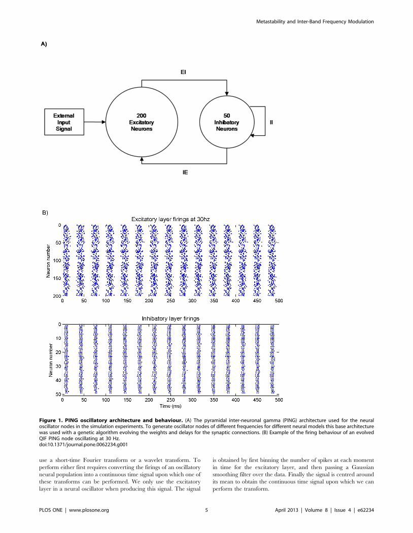
Figure 1b shows a raster plot of an evolved PING oscillator with
regular bursts of firing in the excitatory layer at 30 Hz.
Extraction of intermittent frequency strandsThe work presented in this paper aims at assessing the
correlation between the fluctuating frequencies in different neural
oscillators that are connected together in a network. In order to
achieve this we first need to extract the instantaneous frequency
responses for each neural oscillator at each moment in time during
a simulation. The standard techniques for doing this are to either
Metastability and Inter-Band Frequency Modulation
PLOS ONE | www.plosone.org 4 April 2013 | Volume 8 | Issue 4 | e62234
use a short-time Fourier transform or a wavelet transform. To
perform either first requires converting the firings of an oscillatory
neural population into a continuous time signal upon which one of
these transforms can be performed. We only use the excitatory
layer in a neural oscillator when producing this signal. The signal
is obtained by first binning the number of spikes at each moment
in time for the excitatory layer, and then passing a Gaussian
smoothing filter over the data. Finally the signal is centred around
its mean to obtain the continuous time signal upon which we can
perform the transform.
Figure 1. PING oscillatory architecture and behaviour. (A) The pyramidal inter-neuronal gamma (PING) architecture used for the neuraloscillator nodes in the simulation experiments. To generate oscillator nodes of different frequencies for different neural models this base architecturewas used with a genetic algorithm evolving the weights and delays for the synaptic connections. (B) Example of the firing behaviour of an evolvedQIF PING node oscillating at 30 Hz.doi:10.1371/journal.pone.0062234.g001
Metastability and Inter-Band Frequency Modulation
PLOS ONE | www.plosone.org 5 April 2013 | Volume 8 | Issue 4 | e62234
Both Fourier and wavelet based approaches for extracting the
time-frequency information from a signal suffer from shortcomings
due to the time-frequency uncertainty principle. A Gabor wavelet
transform has been chosen for use in this work, because the
responses of Gabor wavelets have optimal properties with respect
to the time-frequency uncertainty principle [41]. The Gabor
wavelet used had a centre frequency of 0.6 Hz and was applied
with a continuous wavelet transform using scales from 1 to 100 in
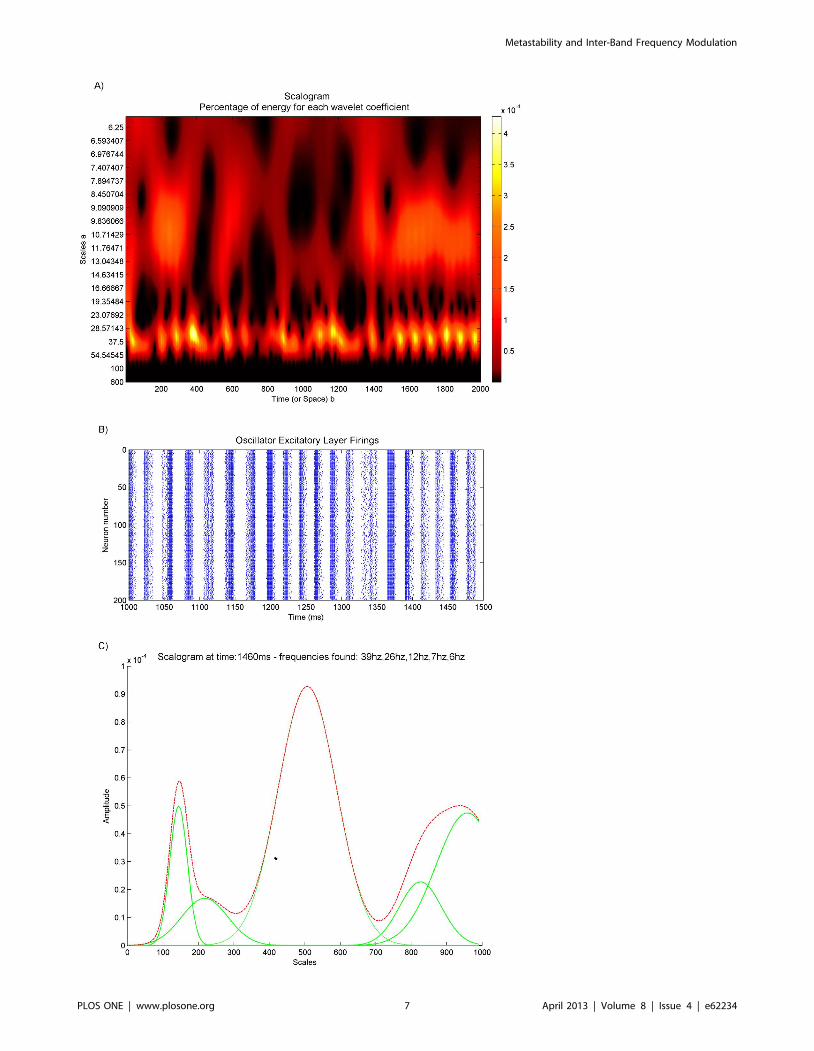
increments of 0.1, and a delta of 0.001. Figure 2a shows the
scalogram of a wavelet transform taken from the excitatory layer
of a neural oscillator in one of the experiments. In this experiment,
as in all others, the oscillator was placed in a network with 9 other
oscillators, each oscillating at a different intrinsic frequency. There
is a given probability of connecting each oscillator to another in
the network, and a given synaptic connection weight for the
connections formed between oscillators. Both connection proba-
bility and synaptic weight are unique to each experimental run.
Figure 2b shows a raster plot of the firing behaviour of the same
excitatory layer between time points 1000 ms and 1500 ms in the
simulation. It can be seen that the spacing of the bursts of firing
between 1050 ms and 1150 ms is wider and thus at a different
slower frequency to the spacing of the bursts of firing between
1200 ms and 1275 ms. The wavelet response to the slow and then
faster bursting can be seen as a difference from low to high
frequency on the scalogram in the same temporal area and around
the frequency range from 30 Hz–50 Hz. These responses are
deviations from the regular 33 Hz bursting that the PING
oscillator was evolved to fire at and are due to the interaction
with the other oscillator nodes.
The Gabor wavelet produces a blurred impulse response
around given frequency responses at each point in time. The
blurring from a Gabor wavelet is in the form of a Gaussian [41], as
illustrated by a time slice at time point 1460 ms shown in figure 2c
taken from the scalogram in figure 2a. Further techniques have to
be applied to the transformed data in order to extract the
instantaneous frequency information. Standard ridge and skeleton
methods do not perform well when there are many components,
some of which remain very close for a while and separate again, or
when they can die out, or when new ones can appear from
nowhere [42]. As can be seen by the scalogram in figure 2a the
data in the work presented here is of this type. Drawing upon the
Gaussian nature of the impulse response from the Gabor wavelet,
we apply a technique of fitting a sum-of-Gaussians model to the
transformed data at each point in time [41]. Figure 2c shows such
a fitting. Identifying the means and magnitudes of the means of the
fitted Gaussians gives the instantaneous frequencies and their
amplitudes respectively.
The next stage in preprocessing the data requires forming a
time series of the instantaneous frequencies as they fluctuate over
time, what we call a strand. These fluctuating frequency responses
may also be intermittent due to the frequency response dropping
out and starting again. Zero values are substituted into the time
series strands during the drop out moments to identify the fact that
there is no frequency response at those times. There may be many
coexisting frequencies for each neural oscillator at each time point
in a simulation, and therefore many coexisting strands. To obtain
these strands, after the instantaneous frequencies at each point in
time for an oscillator are calculated, the movement of each
frequency is tracked over time so as to link them together into a
single time series fragment.
The algorithm for forming the frequency time series strands has
three parts. The first part is simply to sequence the nearest
frequencies in time into a strand as follows:
T = start_time.
while T is not equal to end_time.
For each unassigned instantaneous frequency at time point T
create a new strand containing that frequency.
T = T+1.
while there are strands and frequencies within the distance
limit L.
Find the strand at time point T-1 with the closest frequency to
one of the instantaneous frequencies at time point T.
If the frequency is within limit L add the frequency to the strand
and remove the strand from further consideration until the next
iteration.
endend
Further to this, we need to cope with bifurcations in the
oscillator behaviour when an oscillator in a particular state A1,
flips to another state B1, and then flips again to a state A2 such
that states A1 and A2 have the same number of coexisting
frequencies and these frequencies have approximately the same
values. Hence the system is returning to its original state (A1) after
the middle state B1. In each state there may be several coexistent
frequency strands. We wish the strands in the original state A1 and
its return state A2 after the middle state, to be stitched together so
as to maximize the strand length and as a result the correlation.
The distance between the frequencies in the strands in the state A1
and state A2 may be near enough within a limit L to make a direct
match as in the previous algorithm, due to the fact that there is a
close continuation between the two. However, there are situations
in which the values of the frequencies in A2 are not near enough
for direct matching, but instead have values similar to how state
A1 would have been at that time if the bifurcations had not
occurred and state A1 had instead continued developing. That is
to say, whilst being the same state as A1, state A2 is in a later stage
of development. In such a situation we use regression to project
where the frequencies of strands in the original state A1 would
have progressed to, and match these projections to the frequencies
of the strands in A2. We apply a maximum frequency distance
limit L as before on this projected matching.
In order to stitch states in this way, we first group all strands
together which share the same start time so as to identify them as
being in the same state. The state matching algorithm then
preferentially matches states nearest to each other whose strands
have the closest frequencies or projected frequencies. There is a
maximum time limit between states for which we allow such
stitching to occur. In order to get the best matching between states,
we first perform the algorithm with the constraint that stitched
states must contain the same number of strands, and then perform
the algorithm again without this constraint.
After the state stitching has been carried out we extract the
individual strands that are contained within the states, as we only
consider pairs of individual strands during correlation. The strands
are time series of fluctuating frequencies sequenced by closeness.
Each strand will have a start and end and may contain zero values
in its time series where the frequency dropped out due to a
bifurcation.
Mean Intermittent frequency correlationFor each pair of oscillators, m and n, there is a collection of
fluctuating frequency strands scattered over the frequency domain
and stretching over time. We correlate each strand in oscillator m
with each strand in oscillator n, for all oscillator combinations in
the network. We do this by passing a 100 millisecond window over
time in incremental steps of 1 millisecond. In each of these
Metastability and Inter-Band Frequency Modulation
PLOS ONE | www.plosone.org 6 April 2013 | Volume 8 | Issue 4 | e62234
Metastability and Inter-Band Frequency Modulation
PLOS ONE | www.plosone.org 7 April 2013 | Volume 8 | Issue 4 | e62234
windows we take the time series data in that window for all pairs of
strands i and j, where i and j are from different oscillators m and n
respectively. For each pair of windowed strands we then remove
time points from each strand where both strands do not have a
response at that time point in the window, or when both the
frequencies in the strands at one time point are the same as at the
previous time point. This results in two time series strands for the
window at time t, wm,i(t) and wn,j (t). Both are the same length and
are potentially shorter than the window size. Each time series
contains only data where both original strands have a frequency
response and they are both fluctuating. We then correlate these
two series. We select only correlations where the coefficient is
greater than or equal to 0.5 or the coefficient of the anti-
correlation is less than or equal to 20.5, and the p-value for either
is less than 0.05. By randomizing the order of one of the series and
performing the same correlation and selection process we obtain a
phantom correlation. We use phantom correlations to evaluate the
importance of the measure of real correlation found. For both
types of correlation we calculate the mean intermittent frequency
correlation as follow:
MIFC~1
tmax{100
Xtmax{100
t
Xn
Xm=n
XI(t)
i
XJ(t)
j
W (t)
100coef � wm,i(t),wn,j(t)
� ��� ��
Where n and m are oscillators, I(t) and J(t) are the total number
of strands in the window at time t for each oscillator respectively,
and i and j are particular strands within each oscillator. coef*
defines the value of a significant correlation coefficient as
previously described. W(t) is the length of the two series wm,i(t)
and wn,j (t), that only contain time points that have a fluctuating
frequency response in both original windowed strands. 100 is the
length of the window. Thus the significant correlation coefficient is
normalized according to the length of the two series in that
window. t is the time of the particular window and tmax is the length
of the simulation time. The metric calculates all pairwise
significant frequency correlations between all oscillators, normal-
izes them by their length, and averages them over time.
Synchronisation metricAll the simulations in this work consisted of 10 neural oscillators
connected together. Each neural oscillator consisted of an
excitatory layer and an inhibitory layer. We only calculated
synchrony for the excitatory neuron layers in the oscillators. The
spikes of each neuron in each excitatory layer were binned over
time, and then a Gaussian smoothing filter was passed over the
binned data to produce a continuous time varying signal.
Following this, we performed a Hilbert transform on the mean-
centred filtered signal in order to identify its phase. No band-pass
filtering was performed during this process. The synchrony at time
t was then calculated as follows:
Q(t)~1
N
XN
j
ehj tð Þi
����������
Q~1
tMax
Xt
Q(t)
where hj(t) is the phase at time t of oscillatory population j. i is the
square root of -1. N is the number of oscillators, and tmax is the
length of time of the simulation.
Coalition entropyCoalition entropy measures the variety of metastable states
entered by a system of oscillators. We only calculated coalition
entropy for the excitatory neuron layers in the oscillators. As with
the synchrony metric, we calculated the phase of each oscillator at
each time point t using a Hilbert transform. We then performed
clustering at each time point by picking the two most synchronous
oscillators/coalitions using the first equation defined for the
synchrony metric. Once a pair was identified they were joined to
form a new coalition and the new coalitions mean complex
exponential phase was calculated for use in the future most
synchronous pair selection process. A threshold of 0.05 from full
synchrony was used to limit the cluster merging. The process was
repeated until no oscillators/coalitions fell within the threshold to
allow merging into a new coalition.
Having identified the synchronous coalitions at each point in
time we calculated the probability p(s) of each coalition occurring
from the number of times it appeared throughout the simulation.
The coalition entropy Hc was then calculated as follows:
Hc~�1
log2 jSjXs[S
p sð Þlog2 p sð Þð Þ
where |S| is the number of possible coalitions given the number of
oscillators in the system.
Hardware accelerationEach of our simulations required 10 neural PING nodes each of
250 neurons, resulting in 2500 neurons and <880,000 synapses,
and entailing an immense computational burden across the entire
parameter space sweep in our experiments. To cope with this, we
used the NeMo neural network simulator, which processes
neurons concurrently on general purpose graphics processing
units (GPUs) [43]. The NeMo software permits the addition of
user plugins for neural models, which allowed us to implement
both QIF and HH models for the NeMo simulator facilitating the
work presented here.
Results
We performed a series of experimental simulations in each of
which 10 neural PING oscillators were chosen from the set we had
evolved with intrinsic frequencies ranging from 30 Hz to 50 Hz.
Figure 2. Extraction of frequencies from population firings (A) Scalogram of the excitatory layer of a neural PING node that hasbeen connected to 9 other nodes each oscillating at a different frequency. (B) Firing behaviour of the same excitatory layer between1000 ms to 1500 ms in the simulation. Note how the spacing in between the burst of firing is reflected as different frequencies in the scalogram inpanel A. (C) Time slice of the scalogram in panel A taken at 1460 ms. The red line shows the time slice and the green lines show different Gaussians,the sum of which fits the red line.doi:10.1371/journal.pone.0062234.g002
Metastability and Inter-Band Frequency Modulation
PLOS ONE | www.plosone.org 8 April 2013 | Volume 8 | Issue 4 | e62234
The probability of one oscillator providing neural input to another
was determined with a given probability P. The probability P was
the same for all oscillator to oscillator connections in the same
experimental simulation. Given that a connection was established
from oscillator n to oscillator m the excitatory neurons in oscillator
n would form synaptic connections to the excitatory neurons in
oscillator m. The number of synaptic connections formed was 20
percent of the 40000 possible synaptic connections from the 200
excitatory neurons in oscillator n to the 200 excitatory neurons in
oscillator m. For all synaptic connections formed the weight of the
synapse was set to W. The value for W and P were randomly
chosen at the beginning of each experimental simulation from a
uniform distribution between 0 and 1. 250 simulations were
performed for the QIF neural model and 250 simulations for the
HH neural model. As the weight and connection probability for
each simulation were chosen at random these data points are
scattered throughout the space, the 250 simulations thus constitute
a scattered sweep of weight and the inter-oscillator network
connection sparsity. Figures 3, 4, 5 and 6 show various measures
taken from these 250 simulations of QIF and HH neuron models.
These are analysed and discussed in detail below. In each of these
figures a surface has been fitted to the underlying trend of the 250
data point for each measure depicted. The original scatter plots for
the 250 data points of each measure are included in the supporting
information (figures S1, S2, S4, S4 respectively).
Throughout each simulation external stimulus input was
provided to each neural oscillator from a Poisson process with
parameter l= 4.375. For QIF models the inputs were scaled by 8
and for the HH models the inputs were scaled by 15 in order to
provide sufficient stimulus to induce firing. Each experiment was
run for 2000 ms of simulated time. After each experiment, the
firing activity of the excitatory layers in each oscillator was used to
calculate synchrony, coalition entropy and the mean intermittent
frequency correlation as described in the Methods section. The
first 500 ms of each simulation were discarded in the calculation of
these metrics to eliminate initial transients.
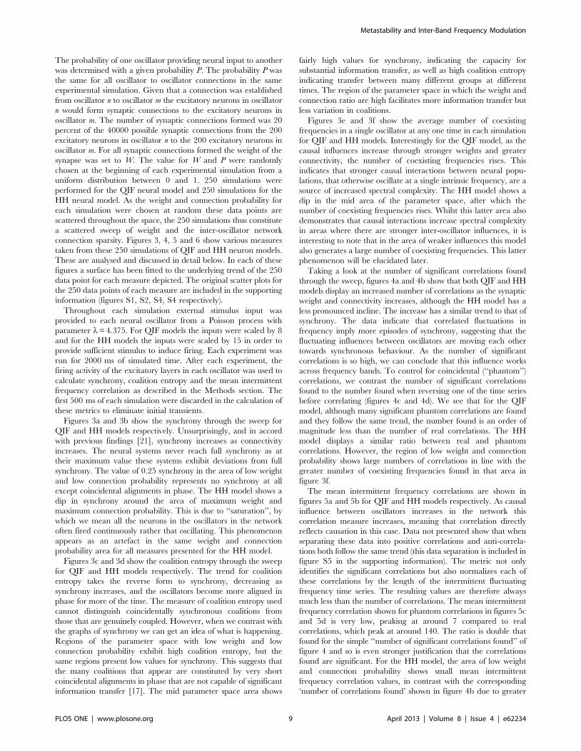
Figures 3a and 3b show the synchrony through the sweep for
QIF and HH models respectively. Unsurprisingly, and in accord
with previous findings [21], synchrony increases as connectivity
increases. The neural systems never reach full synchrony as at
their maximum value these systems exhibit deviations from full
synchrony. The value of 0.25 synchrony in the area of low weight
and low connection probability represents no synchrony at all
except coincidental alignments in phase. The HH model shows a
dip in synchrony around the area of maximum weight and
maximum connection probability. This is due to ‘‘saturation’’, by
which we mean all the neurons in the oscillators in the network
often fired continuously rather that oscillating. This phenomenon
appears as an artefact in the same weight and connection
probability area for all measures presented for the HH model.
Figures 3c and 3d show the coalition entropy through the sweep
for QIF and HH models respectively. The trend for coalition
entropy takes the reverse form to synchrony, decreasing as
synchrony increases, and the oscillators become more aligned in
phase for more of the time. The measure of coalition entropy used
cannot distinguish coincidentally synchronous coalitions from
those that are genuinely coupled. However, when we contrast with
the graphs of synchrony we can get an idea of what is happening.
Regions of the parameter space with low weight and low
connection probability exhibit high coalition entropy, but the
same regions present low values for synchrony. This suggests that
the many coalitions that appear are constituted by very short
coincidental alignments in phase that are not capable of significant
information transfer [17]. The mid parameter space area shows
fairly high values for synchrony, indicating the capacity for
substantial information transfer, as well as high coalition entropy
indicating transfer between many different groups at different
times. The region of the parameter space in which the weight and
connection ratio are high facilitates more information transfer but
less variation in coalitions.
Figures 3e and 3f show the average number of coexisting
frequencies in a single oscillator at any one time in each simulation
for QIF and HH models. Interestingly for the QIF model, as the
causal influences increase through stronger weights and greater
connectivity, the number of coexisting frequencies rises. This
indicates that stronger causal interactions between neural popu-
lations, that otherwise oscillate at a single intrinsic frequency, are a
source of increased spectral complexity. The HH model shows a
dip in the mid area of the parameter space, after which the
number of coexisting frequencies rises. Whilst this latter area also
demonstrates that causal interactions increase spectral complexity
in areas where there are stronger inter-oscillator influences, it is
interesting to note that in the area of weaker influences this model
also generates a large number of coexisting frequencies. This latter
phenomenon will be elucidated later.
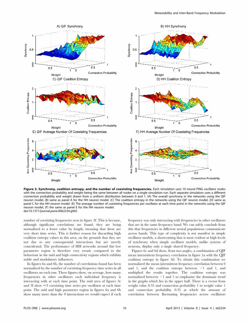
Taking a look at the number of significant correlations found
through the sweep, figures 4a and 4b show that both QIF and HH
models display an increased number of correlations as the synaptic
weight and connectivity increases, although the HH model has a
less pronounced incline. The increase has a similar trend to that of
synchrony. The data indicate that correlated fluctuations in
frequency imply more episodes of synchrony, suggesting that the
fluctuating influences between oscillators are moving each other
towards synchronous behaviour. As the number of significant
correlations is so high, we can conclude that this influence works
across frequency bands. To control for coincidental (‘‘phantom’’)
correlations, we contrast the number of significant correlations
found to the number found when reversing one of the time series
before correlating (figures 4c and 4d). We see that for the QIF
model, although many significant phantom correlations are found
and they follow the same trend, the number found is an order of
magnitude less than the number of real correlations. The HH
model displays a similar ratio between real and phantom
correlations. However, the region of low weight and connection
probability shows large numbers of correlations in line with the
greater number of coexisting frequencies found in that area in
figure 3f.
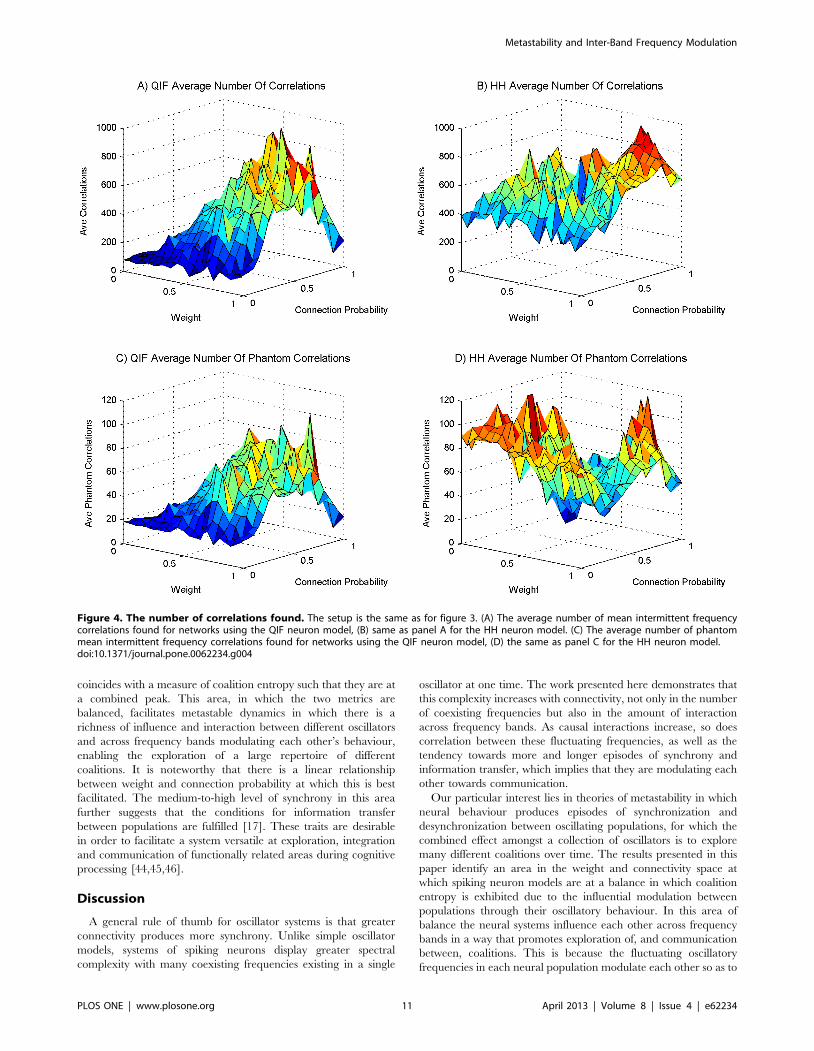
The mean intermittent frequency correlations are shown in
figures 5a and 5b for QIF and HH models respectively. As causal
influence between oscillators increases in the network this
correlation measure increases, meaning that correlation directly
reflects causation in this case. Data not presented show that when
separating these data into positive correlations and anti-correla-
tions both follow the same trend (this data separation is included in
figure S5 in the supporting information). The metric not only
identifies the significant correlations but also normalizes each of
these correlations by the length of the intermittent fluctuating
frequency time series. The resulting values are therefore always
much less than the number of correlations. The mean intermittent
frequency correlation shown for phantom correlations in figures 5c
and 5d is very low, peaking at around 7 compared to real
correlations, which peak at around 140. The ratio is double that
found for the simple ‘‘number of significant correlations found’’ of
figure 4 and so is even stronger justification that the correlations
found are significant. For the HH model, the area of low weight
and connection probability shows small mean intermittent
frequency correlation values, in contrast with the corresponding
‘number of correlations found’ shown in figure 4b due to greater
Metastability and Inter-Band Frequency Modulation
PLOS ONE | www.plosone.org 9 April 2013 | Volume 8 | Issue 4 | e62234
number of coexisting frequencies seen in figure 3f. This is because,
although significant correlations are found, they are being
normalized to a lesser value by length, meaning that these are
very short time series. This is further reason for discarding high
coalition entropy values in this area, on the grounds that they are
not due to any consequential interactions but are merely
coincidental. The performance of HH networks around this low
parameter region is therefore very erratic compared to the
behaviour in the mid and high connectivity regions which exhibits
stable and modulatory influences.
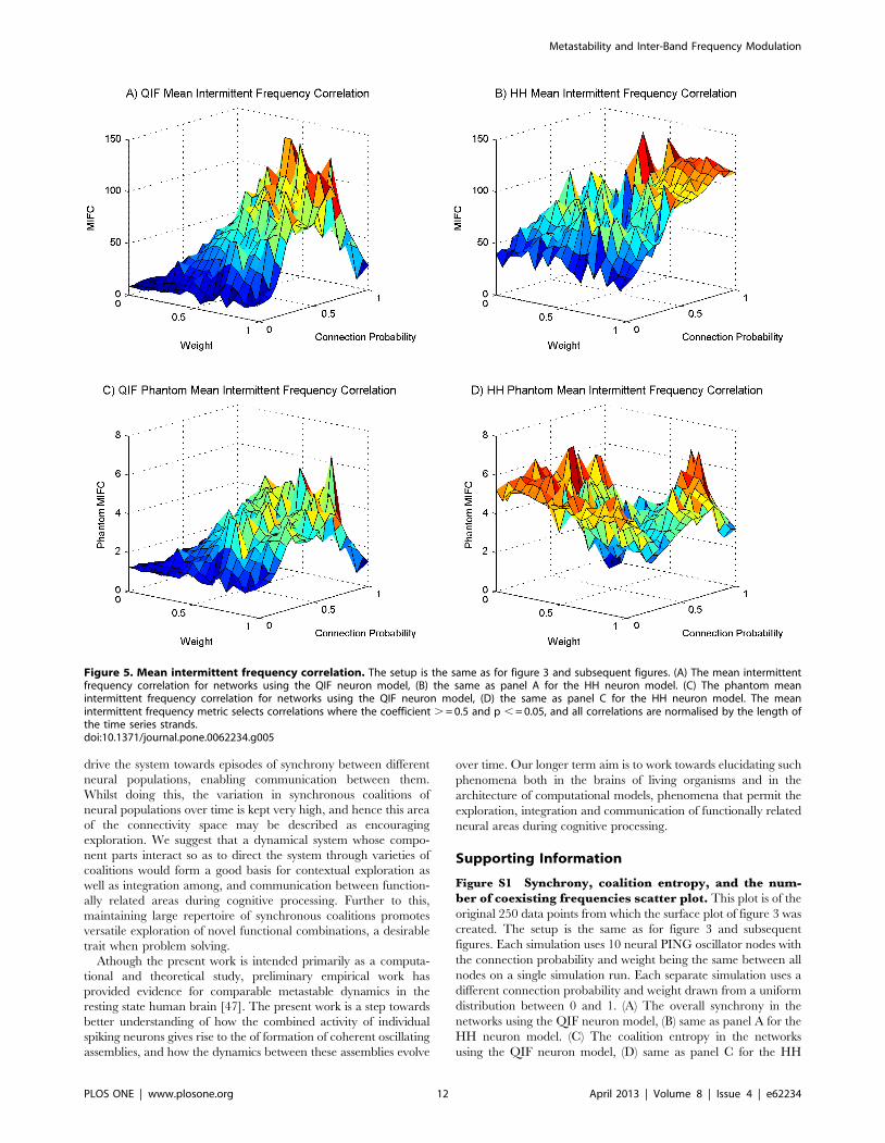
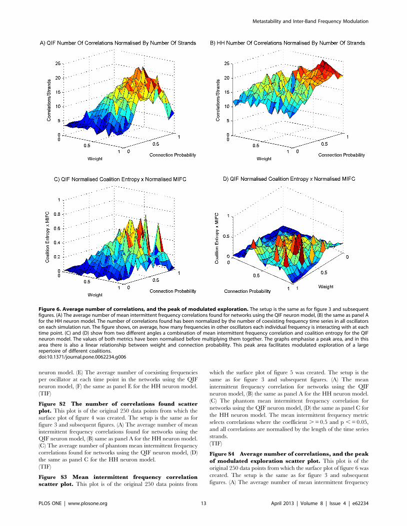
In figures 6a and 6b, the number of correlations found has been
normalized by the number of coexisting frequency time series in all
oscillators on each run. These figures show, on average, how many
frequencies in other oscillators each individual frequency is
interacting with at each time point. The mid area of figures 3e
and 3f show <3 coexisting time series per oscillator at each time
point. The mid and high parameter region in figures 6a and 6b
show many more than the 9 interactions we would expect if each
frequency was only interacting with frequencies in other oscillators
that are in the same frequency band. We can safely conclude from
this that frequencies in different neural populations communicate
across bands. This type of complexity is not manifest in simple
oscillator models, a shortcoming that is most evident at high levels
of synchrony when simple oscillator models, unlike systems of
neurons, display only a single shared frequency.
Figures 6c and 6d show, from two angles, a combination of QIF
mean intermittent frequency correlation in figure 5a with the QIF
coalition entropy in figure 3d. To obtain this combination we
normalized the mean intermittent frequency correlation between 0
and 1, and the coalition entropy between 21 and 1, and
multiplied the results together. The coalition entropy was
normalized between 21 and 1 to emphasize the dominant trend
in the graphs which lies in the upper half. There is a vector from
weight value 0.35 and connection probability 1 to weight value 1
and connection probability 0.35 at which the amount of
correlation between fluctuating frequencies across oscillators
Figure 3. Synchrony, coalition entropy, and the number of coexisting frequencies. Each simulation uses 10 neural PING oscillator nodeswith the connection probability and weight being the same between all nodes on a single simulation run. Each separate simulation uses a differentconnection probability and weight drawn from a uniform distribution between 0 and 1. (A) The overall synchrony in the networks using the QIFneuron model, (B) same as panel A for the HH neuron model. (C) The coalition entropy in the networks using the QIF neuron model, (D) same aspanel C for the HH neuron model. (E) The average number of coexisting frequencies per oscillator at each time point in the networks using the QIFneuron model, (F) the same as panel E for the HH neuron model.doi:10.1371/journal.pone.0062234.g003
Metastability and Inter-Band Frequency Modulation
PLOS ONE | www.plosone.org 10 April 2013 | Volume 8 | Issue 4 | e62234
coincides with a measure of coalition entropy such that they are at
a combined peak. This area, in which the two metrics are
balanced, facilitates metastable dynamics in which there is a
richness of influence and interaction between different oscillators
and across frequency bands modulating each other’s behaviour,
enabling the exploration of a large repertoire of different
coalitions. It is noteworthy that there is a linear relationship
between weight and connection probability at which this is best
facilitated. The medium-to-high level of synchrony in this area
further suggests that the conditions for information transfer
between populations are fulfilled [17]. These traits are desirable
in order to facilitate a system versatile at exploration, integration
and communication of functionally related areas during cognitive
processing [44,45,46].
Discussion
A general rule of thumb for oscillator systems is that greater
connectivity produces more synchrony. Unlike simple oscillator
models, systems of spiking neurons display greater spectral
complexity with many coexisting frequencies existing in a single
oscillator at one time. The work presented here demonstrates that
this complexity increases with connectivity, not only in the number
of coexisting frequencies but also in the amount of interaction
across frequency bands. As causal interactions increase, so does
correlation between these fluctuating frequencies, as well as the
tendency towards more and longer episodes of synchrony and
information transfer, which implies that they are modulating each
other towards communication.
Our particular interest lies in theories of metastability in which
neural behaviour produces episodes of synchronization and
desynchronization between oscillating populations, for which the
combined effect amongst a collection of oscillators is to explore
many different coalitions over time. The results presented in this
paper identify an area in the weight and connectivity space at
which spiking neuron models are at a balance in which coalition
entropy is exhibited due to the influential modulation between
populations through their oscillatory behaviour. In this area of
balance the neural systems influence each other across frequency
bands in a way that promotes exploration of, and communication
between, coalitions. This is because the fluctuating oscillatory
frequencies in each neural population modulate each other so as to
Figure 4. The number of correlations found. The setup is the same as for figure 3. (A) The average number of mean intermittent frequencycorrelations found for networks using the QIF neuron model, (B) same as panel A for the HH neuron model. (C) The average number of phantommean intermittent frequency correlations found for networks using the QIF neuron model, (D) the same as panel C for the HH neuron model.doi:10.1371/journal.pone.0062234.g004
Metastability and Inter-Band Frequency Modulation
PLOS ONE | www.plosone.org 11 April 2013 | Volume 8 | Issue 4 | e62234
drive the system towards episodes of synchrony between different
neural populations, enabling communication between them.
Whilst doing this, the variation in synchronous coalitions of
neural populations over time is kept very high, and hence this area
of the connectivity space may be described as encouraging
exploration. We suggest that a dynamical system whose compo-
nent parts interact so as to direct the system through varieties of
coalitions would form a good basis for contextual exploration as
well as integration among, and communication between function-
ally related areas during cognitive processing. Further to this,
maintaining large repertoire of synchronous coalitions promotes
versatile exploration of novel functional combinations, a desirable
trait when problem solving.
Athough the present work is intended primarily as a computa-
tional and theoretical study, preliminary empirical work has
provided evidence for comparable metastable dynamics in the
resting state human brain [47]. The present work is a step towards
better understanding of how the combined activity of individual
spiking neurons gives rise to the of formation of coherent oscillating
assemblies, and how the dynamics between these assemblies evolve
over time. Our longer term aim is to work towards elucidating such
phenomena both in the brains of living organisms and in the
architecture of computational models, phenomena that permit the
exploration, integration and communication of functionally related
neural areas during cognitive processing.
Supporting Information
Figure S1 Synchrony, coalition entropy, and the num-ber of coexisting frequencies scatter plot. This plot is of the
original 250 data points from which the surface plot of figure 3 was
created. The setup is the same as for figure 3 and subsequent
figures. Each simulation uses 10 neural PING oscillator nodes with
the connection probability and weight being the same between all
nodes on a single simulation run. Each separate simulation uses a
different connection probability and weight drawn from a uniform
distribution between 0 and 1. (A) The overall synchrony in the
networks using the QIF neuron model, (B) same as panel A for the
HH neuron model. (C) The coalition entropy in the networks
using the QIF neuron model, (D) same as panel C for the HH
Figure 5. Mean intermittent frequency correlation. The setup is the same as for figure 3 and subsequent figures. (A) The mean intermittentfrequency correlation for networks using the QIF neuron model, (B) the same as panel A for the HH neuron model. (C) The phantom meanintermittent frequency correlation for networks using the QIF neuron model, (D) the same as panel C for the HH neuron model. The meanintermittent frequency metric selects correlations where the coefficient . = 0.5 and p , = 0.05, and all correlations are normalised by the length ofthe time series strands.doi:10.1371/journal.pone.0062234.g005
Metastability and Inter-Band Frequency Modulation
PLOS ONE | www.plosone.org 12 April 2013 | Volume 8 | Issue 4 | e62234
neuron model. (E) The average number of coexisting frequencies
per oscillator at each time point in the networks using the QIF
neuron model, (F) the same as panel E for the HH neuron model.
(TIF)
Figure S2 The number of correlations found scatterplot. This plot is of the original 250 data points from which the
surface plot of figure 4 was created. The setup is the same as for
figure 3 and subsequent figures. (A) The average number of mean
intermittent frequency correlations found for networks using the
QIF neuron model, (B) same as panel A for the HH neuron model.
(C) The average number of phantom mean intermittent frequency
correlations found for networks using the QIF neuron model, (D)
the same as panel C for the HH neuron model.
(TIF)
Figure S3 Mean intermittent frequency correlationscatter plot. This plot is of the original 250 data points from
which the surface plot of figure 5 was created. The setup is the
same as for figure 3 and subsequent figures. (A) The mean
intermittent frequency correlation for networks using the QIF
neuron model, (B) the same as panel A for the HH neuron model.
(C) The phantom mean intermittent frequency correlation for
networks using the QIF neuron model, (D) the same as panel C for
the HH neuron model. The mean intermittent frequency metric
selects correlations where the coefficient . = 0.5 and p , = 0.05,
and all correlations are normalised by the length of the time series
strands.
(TIF)
Figure S4 Average number of correlations, and the peakof modulated exploration scatter plot. This plot is of the
original 250 data points from which the surface plot of figure 6 was
created. The setup is the same as for figure 3 and subsequent
figures. (A) The average number of mean intermittent frequency
Figure 6. Average number of correlations, and the peak of modulated exploration. The setup is the same as for figure 3 and subsequentfigures. (A) The average number of mean intermittent frequency correlations found for networks using the QIF neuron model, (B) the same as panel Afor the HH neuron model. The number of correlations found has been normalized by the number of coexisting frequency time series in all oscillatorson each simulation run. The figure shows, on average, how many frequencies in other oscillators each individual frequency is interacting with at eachtime point. (C) and (D) show from two different angles a combination of mean intermittent frequency correlation and coalition entropy for the QIFneuron model. The values of both metrics have been normalised before multiplying them together. The graphs emphasise a peak area, and in thisarea there is also a linear relationship between weight and connection probability. This peak area facilitates modulated exploration of a largerepertoire of different coalitions.doi:10.1371/journal.pone.0062234.g006
Metastability and Inter-Band Frequency Modulation
PLOS ONE | www.plosone.org 13 April 2013 | Volume 8 | Issue 4 | e62234
correlations found normalised by the number of coexisting strands
for networks using the QIF neuron model, (B) the same as panel A
for the HH neuron model. The number of correlations found has
been normalised by the number of coexisting frequency time series
in all oscillators on each simulation run. The figure shows, on
average, how many frequencies in other oscillators each individual
frequency is interacting with at each time point. (C) and (D) show
from two different angles a combination of mean intermittent
frequency correlation and coalition entropy for the QIF neuron
model. The values of both metrics have been normalised before
multiplying them together. The graphs emphasise a peak area, and
in this area there is also a linear relationship between weight and
connection probability. This peak area facilitates modulated
exploration of a large repertoire of different coalitions.
(TIF)
Figure S5 Separation of positive and anti mean inter-mittent frequency correlation. (A) The positive mean
intermittent frequency correlation for the QIF neuron model. (B)
The same as panel A for the HH neuron model. (C) The anti
mean intermittent frequency correlation for the QIF neuron
model. (B) The same as panel C for the HH neuron model.
(TIF)
File S1. Supporting Figure Descriptions.
DOC)
Author Contributions
Conceived and designed the experiments: DB MS. Performed the
experiments: DB. Analyzed the data: DB MS. Contributed reagents/
materials/analysis tools: DB MS. Wrote the paper: DB MS.
References
1. Alonso A, Llinas R (1989) Subthreshold Na+-dependent theta-like rhythmicity instellate cells of entorhinal cortex layer II. Nature 342: 175–177.
2. Ramirez J, Tryba AK, Pea F (2004) Pacemaker neurons and neuronal networks:
an integrative view. Current Opinion in Neurobiology 14(6): 665–674.3. Nyhus E, Curran T (2010) Functional role of gamma and theta oscillations in
episodic memory. Neuroscience and biobehavioral reviews 2010;34(7): 1023–35.4. Buzsaki G, Draguhn A (2004) Neuronal oscillations in cortical networks. Science
(New York, N.Y.) 304(5679): 1926–9.5. McCormick DA, Sejnowski TJ, Steriade M (1993) Thalamocortical oscillations
in the sleeping and aroused brain. Science 262: 679–85.
6. Basar E, Basar-Eroglu C, Karakas S, Schurmann M (2000) Brain oscillations inperception and memory. International Journal of Psychophysiology 35(23): 95–
124.7. Klimesch W (1999) EEG alpha and theta oscillations reflect cognitive and
memory performance: a review and analysis. Brain Research Reviews 29(23):
169–195.8. Pfurtscheller G, Stancak Jr A, Neuper C (1996) Post-movement beta
synchronization. correlate of an idling motor area? Electroencephalographyand Clinical Neurophysiology 98(4): 281–293.
9. Jensen O, Kaiser J, Lachaux J (2007) Human gamma-frequency oscillations
associated with attention and memory. Trends in Neurosciences 30(7): 317–324.10. Miltner WHR, Braun C, Matthias A, Witte H, Taub E (1999) Coherence of
gamma-band EEG activity as a basis for associative learning. Nature 397(6718):434–436.
11. Siegel M, Warden MR, Miller EK (2009) Phase-dependent neuronal coding ofobjects in short-term memory. Proceedings of the National Academy of Sciences
of the United States of America 106(50): 21341–6.
12. Lisman J (2005) The theta/gamma discrete phase code occuring during thehippocampal phase precession may be a more general brain coding scheme.
Hippocampus 2005;15(7): 913–22.13. Fries P, Reynolds JH, Rorie AE, Desimone R (2001) Modulation of oscillatory
neuronal synchronization by selective visual attention. Science 291(5508): 1560–
1563. 2.1.14. Fries P, Schroder J, Roelfsema PR, Singer W, Engel AK (2002) Oscillatory
neuronal synchronization in primary visual cortex as a correlate of stimulusselection. Journal of Neuroscience 22(9): 3739–3754.
15. Steriade M, Jones EG, Llinas RR (1990) Thalamic Oscillations and Signalling.John Wiley and Sons 1990.
16. Fries P (2005) A mechanism for cognitive dynamics: neuronal communication
through neuronal coherence. Trends in cognitive sciences 2005;9(10): 474–80.17. Buehlmann A, Deco G (2010) Optimal Information Transfer in the Cortex
through Synchronization. (K. J. Friston, Ed.) PLoS Computational Biology 6(9).18. Shanahan M (2010) Metastable chimera states in community structured
oscillator networks. Chaos 20(1): 013108.
19. Wildie M, Shanahan M (2012) Metastability and chimera states in modularpulse-coupled oscillator networks. Chaos 22(4): 043131.
20. Breakspear M, Heitmann S, Daffertshofer A (2010) Generative models ofcortical oscillations: neurobiological implications of the kuramoto model. Front
Hum Neurosci 4: 190.21. Bhowmik D, Shanahan M (2012) How Well Do Oscillator Models Capture the
Behaviour of Biological Neurons? Proceedings IJCNN 2012: 1–8.
22. Kuramoto Y (1984) Chemical Oscillations, Waves and Turbulence. Springer-Verlag Berlin 1984.
23. Steriade M (2012) Impact of Network Activities on Neuronal Properties inCorticothalamic Systems. J Neurophysiol 86(1): 1–39.
formation by neuronal synchronization. Brain research reviews, 52(1): 170–82.25. Roopun AK, Kramer M, Carracedo LM, Kaiser M, Davies CH, Traub RD,
Kopell NJ (2008) Period concatenation underlies interactions between gammaand beta rhythms in neocortex. Frontiers in cellular neuroscience, 2(April): 1.
26. Wildie M, Shanahan M (2011) Establishing Communication between Neuronal
Populations through Competitive Entrainment. Frontiers in computational