Metastable Argon Atoms and the Portable … Argon Atoms and the Portable Rydberg Generator: ......

Wesleyan University The Honors College

Metastable Argon Atoms and the

Portable Rydberg Generator:

or, How I Learned To Stop Worrying and Love

Excited Atoms

by

Joshua Houston Gurian

Class of 2004

A thesis submitted to the

faculty of Wesleyan University

in partial fulfillment of the requirements for the

Degree of Bachelor of Arts

with Departmental Honors in Physics

Middletown, Connecticut April, 2004

Abstract

The purpose of this thesis is twofold. I first aim to give an overview of Stark

recurrence spectroscopy of Rydberg atoms suitable for an undergraduate inter-

ested in experimental research in the Morgan Lab. In the second part of the

thesis a new apparatus for metastable production and Stark recurrence spec-

troscopy is introduced, known as the Portable Rydberg Generator. Various

methods for metastable production are discussed and compared from an exper-

imental viewpoint. Finally, initial experimental data of metastable argon from

this new apparatus is presented.

Acknowledgements

They say it takes a village to raise a child, and this thesis has been no excep-

tion. This experiment never would have materialized from paper if not for the

hard work and support of David Boule, Tom Castelli, Bruce Strickland, Dick

Widlansky, Vacek Miglus, Mirek Koziol, and Anna Milardo. They work magic.

There is also a long list of people who have really gone out of their way to

foster my physics education in the lab. I’m greatly indebted to Heric Flores-

Rueda, Len Keeler, David Wright, Jon Lambert, and Thomas Clausen. They

have all been great mentors and kind friends.

I would have lost my sanity in the lab if were not for the good times with

the esteemed Council of Elders. Intown 21, 84 High, 76 Lawn, and 42 Miles.

Hilarity ensues. I have been incredibly lucky to have Marcus Van Lier - Walqui

as my fellow lab-monkey. As the other half of the atomic duo, he’s been a superb

labmate and a true friend.

My parents have been incredibly understanding and encouraging, even when

they’ve said to me, “We don’t understand what it is that you’re doing, but we’re

glad you’re enjoying it.”

And the person who started me on this whole adventure, Professor Tom

Morgan.

Contents

Abstract 1

Acknowledgements 2

Table of Contents 3

List of Figures 5

1 Introduction 8

1.1 Motivation for Study . . . . . . . . . . . . . . . . . . . . . . . . . 8

1.2 Introduction to Rydberg Atoms in Stark Fields . . . . . . . . . . 9

1.2.1 Hydrogen . . . . . . . . . . . . . . . . . . . . . . . . . . . 9

1.2.2 Multi-electron Atoms . . . . . . . . . . . . . . . . . . . . . 19

1.3 Previous Research . . . . . . . . . . . . . . . . . . . . . . . . . . . 20

2 Methodologies of Spectroscopy 22

2.1 Absorption Spectra . . . . . . . . . . . . . . . . . . . . . . . . . . 22

2.2 Fourier Transforms . . . . . . . . . . . . . . . . . . . . . . . . . . 24

2.3 Recurrence Spectra . . . . . . . . . . . . . . . . . . . . . . . . . . 26

2.4 Closed Orbit Theory . . . . . . . . . . . . . . . . . . . . . . . . . 26

Contents 4

3 The Portable Rydberg Generator 29

3.1 Overview of Design . . . . . . . . . . . . . . . . . . . . . . . . . . 29

3.2 Metastable States . . . . . . . . . . . . . . . . . . . . . . . . . . . 32

3.2.1 Metastable Hydrogen . . . . . . . . . . . . . . . . . . . . . 32

3.2.2 Multi-Electron Metastable States . . . . . . . . . . . . . . 35

3.2.3 Methods of Metastable Creation . . . . . . . . . . . . . . . 35

3.3 Electron Sources . . . . . . . . . . . . . . . . . . . . . . . . . . . 37

3.3.1 HeatWave Labs Source . . . . . . . . . . . . . . . . . . . . 37

3.3.2 Southwest Vacuum Devices Source . . . . . . . . . . . . . 38

3.4 Operating Parameters . . . . . . . . . . . . . . . . . . . . . . . . 38

4 Experimental Data and Analysis 42

5 Conclusion and Future Work 46

Appendices

A Stark Frequency Derivation 48

B Hamiltonian Scaling Derivation 53

C Southwest Vacuum Devices Cathode Installation 55

D Properties of Hydrogenic Ellipses 57

E Pictures of the Portable Rydberg Generator 58

Bibliography 61

Index 68

List of Figures

1.1 Diagram of a Bohr atom, a negatively charged electron of mass

m revolving around an infinitely massive nucleus at distance r . . 9

1.2 Illustration of ~A, the Runge-Lenz vector, for an elliptical orbit

around focus F . . . . . . . . . . . . . . . . . . . . . . . . . . . . . 13

1.3 Comparison of (a) Coulomb potential and (b) Coulomb potential

with a linear Stark term . . . . . . . . . . . . . . . . . . . . . . . 15

1.4 First order Stark shift for hydrogen for n = 15 to n = 20 generated

by Eq. (1.27) . . . . . . . . . . . . . . . . . . . . . . . . . . . . . 16

1.5 Parabolic coordinate system. Lines of constant ξ approach −∞,

lines of constant η approach ∞. Rotation through φ about the

z-axis from 0 to 2π. . . . . . . . . . . . . . . . . . . . . . . . . . . 18

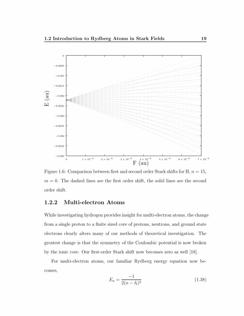
1.6 Comparison between first and second order Stark shifts for H,

n = 15, m = 0. The dashed lines are the first order shift, the

solid lines are the second order shift. . . . . . . . . . . . . . . . . 19

1.7 Example of avoided crossings. Stark Rydberg sodium absorption

calculation from [57]. . . . . . . . . . . . . . . . . . . . . . . . . 21

List of Figures 6

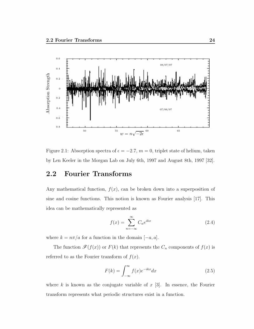
2.1 Absorption spectra of ε = −2.7, m = 0, triplet state of helium,

taken by Len Keeler in the Morgan Lab on July 6th, 1997 and

August 8th, 1997 [32]. . . . . . . . . . . . . . . . . . . . . . . . . 24

2.2 A plot of Eq. (2.6) . . . . . . . . . . . . . . . . . . . . . . . . . . 25

2.3 Fourier transform of Eq. (2.6). . . . . . . . . . . . . . . . . . . . . 25

2.4 Recurrence spectra of Fig. 2.1 taken by Len Keeler in the Morgan

Lab [32] . . . . . . . . . . . . . . . . . . . . . . . . . . . . . . . . 27

3.1 Diagram of PRG . . . . . . . . . . . . . . . . . . . . . . . . . . . 30

3.2 End-cup assembly (Side View) . . . . . . . . . . . . . . . . . . . . 31

3.3 End-cup assembly (Top View) . . . . . . . . . . . . . . . . . . . . 31

3.4 Diagram of charged particle sweepers (Side View) . . . . . . . . . 32

3.5 Diagram of charged particle sweepers (Top View) . . . . . . . . . 33

3.6 Decay routes by spontaneous emission of the first four energy

levels of hydrogen governed by dipole selection rules. . . . . . . . 34

3.7 Diagram of HeatWave TB-198 standard series barium tungsten

dispenser cathode . . . . . . . . . . . . . . . . . . . . . . . . . . . 37

3.8 PRG electron source (Side and Exploded Top View) (SW-Vacuum

Device Configuration) . . . . . . . . . . . . . . . . . . . . . . . . 39

3.9 Southwest Vacuum Devices C−14 cathode diagram . . . . . . . . 40

3.10 Electron source output current (A) of Southwest Vacuum Devices

source as a function of acceleration voltage (V). Electron Source

heaters were at 12 V , drawing ∼2 A. . . . . . . . . . . . . . . . . 41

List of Figures 7

4.1 Experimental argon data illustrating production of metastables by

HeatWave source. Plot of normalized end cup current (arb. units)

as a function of electron acceleration voltage(volts)(07/09/03). . . 42

4.2 Experimental argon data illustrating production of metastables by

Southwest Vacuum Devices source. Plot of normalized end cup

current (arb. units) as a function of electron acceleration volt-

age(volts)(1/23/04). . . . . . . . . . . . . . . . . . . . . . . . . . 43

4.3 Comparison of experimental argon metastable data from Fig. 4.1

and Fig. 4.2. . . . . . . . . . . . . . . . . . . . . . . . . . . . . . . 44

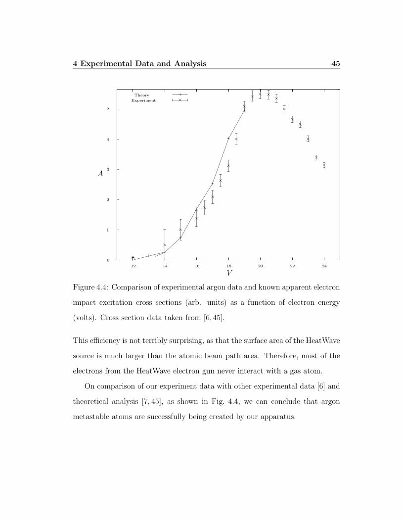
4.4 Comparison of experimental argon data and known apparent elec-

tron impact excitation cross sections (arb. units) as a function of

electron energy (volts). Cross section data taken from [6, 45]. . . . 45

E.1 View of metastable source from the Portable Rydberg Generator

(Southwest Vacuum Devices cathodes) . . . . . . . . . . . . . . . 58

E.2 Wide view of the Portable Rydberg Generator . . . . . . . . . . . 59

E.3 Side view of the Portable Rydberg Generator . . . . . . . . . . . . 60

Chapter 1

Introduction

1.1 Motivation for Study

Highly excited atoms in external perturbations have long been a subject of in-

terest in atomic physics. These highly excited atoms, known as Rydberg atoms,

straddle an interesting place in physics. They represent a quantum mechanical

system extended into a classical domain. One of the driving purposes of this

research has been to try to coalesce these two mechanical formulations. Many of

these systems also exhibit the unique property of being classical chaotic, while

still being solvable in a quantum mechanical regime. This has become known as

“quantum chaos” and is a motivating interest in these systems [30].

The study of Rydberg atoms in static external electric fields, or Stark fields,

has become a extremely interesting problem in physics. Even small deviations

from a Coulomb potential lead to notable changes in the physics of these Rydberg

atoms. Although Rydberg systems have been heavily studied since the 1970s,

the application of recurrence spectroscopy to Rydberg systems is a relatively

1.2 Introduction to Rydberg Atoms in Stark Fields 9

new innovation [18]. The Nobel gases, with a single electron excited out of the

valence shell, provide a complex and interesting system for study. In this thesis

we first look to lay a foundation for investigating Rydberg atoms in Stark fields.

1.2 Introduction to Rydberg Atoms in Stark

Fields

1.2.1 Hydrogen

Hydrogen, with a single proton and a single electron, clearly represents the

simplest classical or quantum mechanical atomic model. Theoretical models of

hydrogen can therefore provide a comparison for more complex atoms and yield

insight into experimental data.

Semi-Classical Hydrogen

The qualitative classical picture of the Rydberg atom is similar to Keplerian

planetary motion. We can quantitatively investigate the classical model of hy-

drogen by first looking at the Bohr model of the atom.

-�r e−

Figure 1.1: Diagram of a Bohr atom, a negatively charged electron of mass m

revolving around an infinitely massive nucleus at distance r

First developed by Bohr in 1913, his theory placed a negative electron in a cir-


cular orbit about a stationary positive nucleus of infinite mass (see Fig 1.1) [18].

Bohr himself made the assumption that the angular momentum in the atom was

quantized in units of ~. In order to align his theory with experimental results,

Bohr also postulated that the atom did not radiate energy continuously, but

only made transitions between states of well defined energies. The angular force

on the electron,

mv2

r(1.1)

can be equated to the attractive force between the proton and electron,

e2

4πε0r2. (1.2)

The angular momentum can be quantized as,

mvr = n~ (1.3)

leading to an expression of the orbital radius of the electron as,

r =4πε0~

2n2

e2m(1.4)

which notably scales as n2.

We can justify the analogy of the electron being in a Kepler orbit by com-

paring the orbital radius to the de Broglie wavelength of the electron. For an

n = 15 excited atom, by Eq. (1.4), our orbital radius is around 119A. We can

compare this distance to the wavelength of the electron, given by the de Broglie

formula,

p =h

λ(1.5)

This puts the de Broglie wavelength at 5.6A, or 0.047 of the electron orbital

radius. The de Broglie wavelength is so small compared to the orbital radius


that we can view this highly excited system as a independent particle very far

from the nucleus, much akin to a Keplerian system. We can consider the electron

in a classical regime when it is far from the nucleus, and no longer as a quantum

system.

If the energy of the electron is written as the sum of the kinetic and Coulombic

potential energies, where

T =1

2mv2 (1.6a)

U = − e2

4πε0r(1.6b)

We can then write the energy as,

E = − e4m

8πε0n2~2(1.7)

clearly scaling as 1/n2. This equation is known as the Rydberg energy equation.

We can now further investigate the first order classical energy shift of the

electron in an electric field by examining the time averaged permanent dipole

moment of hydrogen. It can be noted that any particle in a central field po-

tential has its motion limited to a plane, which we can take to be in polar

coordinates [22]. We can begin by writing down the total energy of the system,

E = 1/2mr2 + 1/2mr2φ2 + U(r) (1.8)

The angular kinetic energy can be expressed in terms of the angular momentum

by noting that

l = mr2φ (1.9)

and therefore

E = 1/2mr2 + 1/2l2

mr2+ U(r) (1.10)


By manipulating this equation we can write,

r =

√

2

m(E − U(r)) − l2

m2r2=

dr

dt(1.11)

or rather,

dt =dr

√

2m

(E − U(r)) − l2

m2r2

(1.12)

Substituting Eq. (1.9), the above equation can be written as

dφ =l

mr2dr√

2m

(E − U(r)) − l2

m2r2

(1.13)

Now is an opportune moment to introduce atomic units (au) in an attempt to

simplify our equations [9]:

me = 1 (1.14a)

a0 = 1 (1.14b)

e = 1 (1.14c)

~ = 1 (1.14d)

6.5761 × 106GHz = 1 (1.14e)

5.137 × 109V/cm = 1 (1.14f)

One should note that Eq. (1.7), our familiar Rydberg energy formula, now be-

comes,

E =−1

2n2(1.15)

Applying Eq. (1.6b) to Eq. (1.13) and integrating both sides yields

φ = cos−1 l/r − m/l√

2mE + m2

l2

(1.16)


As Landau and Lifshitz note [40], the eccentricity of the classical orbit can

be written as

ε =

√

1 +2El2

m(1.17)

We can now apply Eq. (1.14) and Eq. (1.17) to Eq. (1.16) and write our

equation of motion as

l2/r = 1 + εcosφ, (1.18)

an ellipse with one focus at the origin.

We can further investigate the classical hydrogen atom by defining the Runge-

Lenz vector,

~A = ~p × ~L − r (1.19)

It can be shown that the Lenz vector is a constant of motion in Coulombic and

gravitational fields, yet d ~Adt

6= 0 when the potential deviates from 1/r.

•F~Ar

φ

Figure 1.2: Illustration of ~A, the Runge-Lenz vector, for an elliptical orbit around

focus F .

We can now write the average dipole moment of the atom, ~d, as pointing in

the direction of the pericenter, equivalent to the direction of ~A,

< ~d >=< rcosφ > ( ~A/| ~A|) (1.20)

We can integrate over a period of motion to find the magnitude of the dipole

moment,

| < ~d > | =1

τ

∫ τ

0

rcosφdt =1

τ

∫ τ

0

rcosφ1

φdφ (1.21)


By applying Eq. (1.9), and substituting Eq. (1.18) we can rewrite this integral

as

| < ~d > | =l5

2πn3

∫ π

−π

cosφdφ

(1 + εcosφ)3(1.22)

noting that

τ = 2πn3 (1.23)

We can now evaluate the integral Eq. (1.22) as

| < ~d > | =3

2n2ε (1.24)

As Hezel et al note [27], the magnitude of the Runge-Lenz vector is equal to the

eccentricity of the orbit, and therefore

< ~d >=3

2n2 ~A (1.25)

The energy of a dipole in an electric field ~F is simply

E = −~d · ~F (1.26)

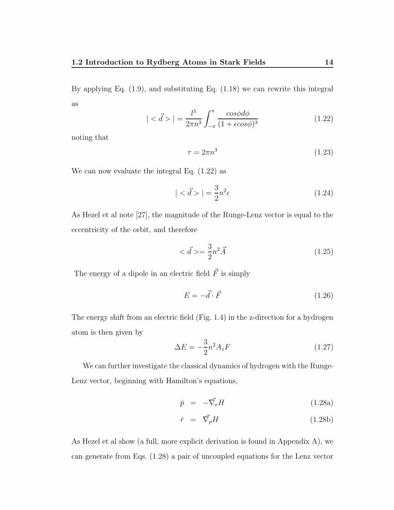
The energy shift from an electric field (Fig. 1.4) in the z-direction for a hydrogen

atom is then given by

∆E = −3

2n2AzF (1.27)

We can further investigate the classical dynamics of hydrogen with the Runge-

Lenz vector, beginning with Hamilton’s equations,

p = − ~∇rH (1.28a)

r = ~∇pH (1.28b)

As Hezel et al show (a full, more explicit derivation is found in Appendix A), we

can generate from Eqs. (1.28) a pair of uncoupled equations for the Lenz vector


(a) (b)

–2

–1.5

–1

–0.5

0.5

1

–10 –8 –6 –4 –2 2 4 6 8 10

PSfrag replacements

V (r)

r

–2

–1.5

–1

–0.5

0.5

1

–10 –8 –6 –4 –2 2 4 6 8 10

PSfrag replacements

r

V (r)

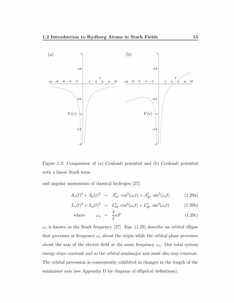
Figure 1.3: Comparison of (a) Coulomb potential and (b) Coulomb potential

with a linear Stark term

and angular momentum of classical hydrogen [27]:

Ax(t)2 + Ay(t)

2 = A2x0 cos2(ωst) + A2

y0 sin2(ωst) (1.29a)

Lx(t)2 + Ly(t)

2 = L2x0 cos2(ωst) + L2

y0 sin2(ωst) (1.29b)

where ωs =3

2nF (1.29c)

ωs is known as the Stark frequency [27]. Eqs. (1.29) describe an orbital ellipse

that precesses at frequency ωs about the origin while the orbital plane precesses

about the axis of the electric field at the same frequency ωs. Our total system

energy stays constant and so the orbital semimajor axis must also stay constant.

The orbital precession is consequently exhibited in changes in the length of the

semiminor axis (see Appendix D for diagram of elliptical definitions).


PSfrag

replacem

ents

E(a

u)

F (au)0

0

5 × 10−7

5×

10−

7

1 × 10−6 1.5 × 10−6 2 × 10−6

−0.0005

−0.001

−0.0015

−0.002

−0.0025

−0.003

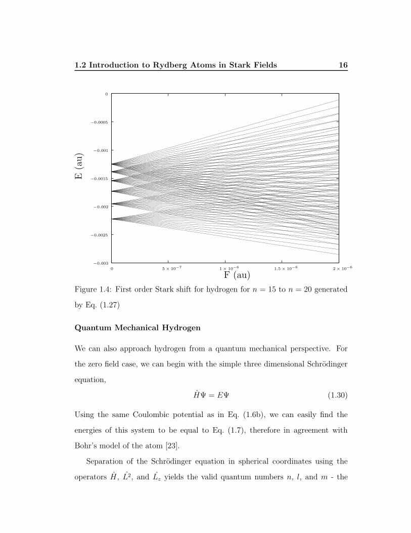
Figure 1.4: First order Stark shift for hydrogen for n = 15 to n = 20 generated

by Eq. (1.27)

Quantum Mechanical Hydrogen

We can also approach hydrogen from a quantum mechanical perspective. For

the zero field case, we can begin with the simple three dimensional Schrodinger

equation,

HΨ = EΨ (1.30)

Using the same Coulombic potential as in Eq. (1.6b), we can easily find the

energies of this system to be equal to Eq. (1.7), therefore in agreement with

Bohr’s model of the atom [23].

Separation of the Schrodinger equation in spherical coordinates using the

operators H, L2, and Lz yields the valid quantum numbers n, l, and m - the


familiar principle, angular, and magnetic quantum numbers, respectively. How-

ever, when an electric field is applied to the atom, and therefore an additional

term added to the potential, the Hamiltonian is no longer separable in spheri-

cal coordinates [18]. Our Hamiltonian is still separable in parabolic coordinates

(Fig. 1.5):

ξ = r + z (1.31a)

η = r − z (1.31b)

φ = tan−1(y/x) (1.31c)

with operators H, L2, and Az, the z-component of the Runge-Lenz vector. Sep-

arating our Hamiltonian in parabolic coordinates yields the quantum numbers

n, n1, n2, and m. These four quantum numbers adhere to the relation

n = n1 + n2 + |m| + 1 (1.32)

and can be re-expressed as n, k, and m when k is written as [2]

k = n1 − n2 (1.33)

The quantum number k is commonly referred to as the electric quantum num-

ber [18]. As Hezel et al note [27], Az can be written as,

Az =(n1 − n2)

n=

k

n(1.34)

The energies to first order of the hydrogen atom in an electric field can then be

written as,

E = − 1

2n2+

3

2nkF (1.35)

A very clean derivation of this can be found in Bethe and Salpeter [4]. This

energy shift as a function of field strength is the same as found in Eq. (1.27).


PSfrag replacements

0

16/5

−16/5

12/5

−12/5

8/5

−8/5

4/5

−4/5

1

2

3

4

−4

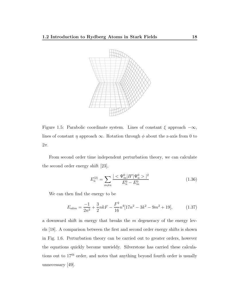
Figure 1.5: Parabolic coordinate system. Lines of constant ξ approach −∞,

lines of constant η approach ∞. Rotation through φ about the z-axis from 0 to

2π.

From second order time independent perturbation theory, we can calculate

the second order energy shift [23],

E(2)n =

∑

m6=n

| < Ψ0m|H ′|Ψ0

n > |2E0

n − E0m

(1.36)

We can then find the energy to be

Enkm =−1

2n2+

3

2nkF − F 2

16n4[17n2 − 3k2 − 9m2 + 19], (1.37)

a downward shift in energy that breaks the m degeneracy of the energy lev-

els [18]. A comparison between the first and second order energy shifts is shown

in Fig. 1.6. Perturbation theory can be carried out to greater orders, however

the equations quickly become unwieldy. Silverstone has carried these calcula-

tions out to 17th order, and notes that anything beyond fourth order is usually

unnecessary [49].


PSfrag

replacem

ents

E(a

u)

F (au)0

0

1 × 10−6 2 × 10−6 3 × 10−6 4 × 10−6 5 × 10−6 6 × 10−6 7 × 10−6

−0.0005

−0.001

−0.0015

−0.002

−0.0025

−0.003

−0.0035

−0.004

−0.0045

−0.005

Figure 1.6: Comparison between first and second order Stark shifts for H, n = 15,

m = 0. The dashed lines are the first order shift, the solid lines are the second

order shift.

1.2.2 Multi-electron Atoms

While investigating hydrogen provides insight for multi-electron atoms, the change

from a single proton to a finite sized core of protons, neutrons, and ground state

electrons clearly alters many of our methods of theoretical investigation. The

greatest change is that the symmetry of the Coulombic potential is now broken

by the ionic core. Our first-order Stark shift now becomes zero as well [18].

For multi-electron atoms, our familiar Rydberg energy equation now be-

comes,

En =−1

2(n − δl)2(1.38)

1.3 Previous Research 20

where δl is an empirically determined, l dependent number known as the quan-

tum defect. This quantum defect also represents a phase shift in the quantum

wave-function of the atom [26, 36].

Due to the finite sized core of the atom, n1 is no longer a good quantum

number and therefore our atom is not separable in parabolic coordinates. The

greatest implication of n1 no longer being a good quantum number is a coupling

between the red (down-shifted) and blue (up-shifted) states of the atom [18].

As a result, avoided crossings exist in the energy spectra of non-hydrogenic

atoms [50]. These avoided crossings alter the classical dynamics of Rydberg

atoms and provide the deviations from the simple hydrogenic dynamics derived

above. A powerful technique for understanding the dynamics of highly excited

multi-electron atoms is closed orbit theory, which will be discussed in Sec. 2.4.

1.3 Previous Research

Previous research in the Morgan Lab has focused on Rydberg helium [32,34–36]

and Rydberg argon [16,33]. Much work by other groups has been conducted on

the alkali metals, both experimentally and theoretically [47, 57]. Our lab next

looks to investigate excited xenon in an electric field. Research into Rydberg

xenon seems to have first been undertaken by Stebbings et al in 1975 [51, 56].

However, this work was done only for the zero-field case. Other previous work

on xenon has primarily been done by Knight and Wang [37, 38, 54] and Ernst

et al [15]. Knight and Wang’s research is primarily at zero-field [37, 54], with

one investigation of xenon in an electric field for a small energy range around

n = 17 [38]. Ernst et al have only investigated the n range between 14 and 21.

1.3 Previous Research 21

Figure 1.7: Example of avoided crossings. Stark Rydberg sodium absorption

calculation from [57].

Warntjes et al have previously investigated the decay paths of autoionizing Ry-

dberg xenon Stark states [55]. Optogalvanic spectroscopy has also been done on

Rydberg xenon for the zero-field case [39]. In the next chapter we will introduce

a powerful method of spectral investigation known as recurrence spectroscopy.

No previously published recurrence spectra have been taken for xenon.

Chapter 2

Methodologies of Spectroscopy

2.1 Absorption Spectra

Recurrence spectroscopy begins with first taking absorption spectra. An atom

absorbs energy at specific quantized energy levels, and absorption spectra such

as Fig. 2.1 represents a plot of the available energy levels for helium over the

energy range from n = 19 to n = 30.

As we add an external electric field to our system in our experiment, the

total system energy changes accordingly,

H =p2

2− 1

r+ Fz (2.1)

However, we can scale our Hamiltonian variables r and p so that our Hamiltonian

is invariant in an electric field. As Keeler describes [32], we can find the scaling

2.1 Absorption Spectra 23

variables,

r = F−1/2r (2.2a)

p = F 1/4p (2.2b)

z = F−1/2z. (2.2c)

We can fold these ideas into a scaled energy relation, which we will refer to as

epsilon. Our scaled energy is then defined as

ε = E/√

F (2.3)

A full derivation can be found in Appendix B. For a given ε our system Hamil-

tonian is now completely independent of the external electric field applied to it.

We therefore scale our absorption spectroscopy accordingly, altering our electric

field and laser energy to keep ε constant. This holds the classical dynamics of

the system constant.

Our spectroscopy is conducted using the second harmonic of a pulsed 1064nm

Nd:YAG (Neodymium doped Yttrium Aluminum Garnet) laser pumping a home-

made dye laser. The light from the dye laser is then sent through a doubling

crystal. This method gives us a laser bandwidth of less than 0.5 cm−1 with a

wide tunable range over multiple tens of wavenumbers [32]. Selection of the mag-

netic angular momentum state (quantum number m) investigated is dependent

on the polarization of the laser with respect to the electric field. Laser polariza-

tion parallel to the applied electric field corresponds to m = 0 and polarization

perpendicular to the field yields m = 1 excitation [16].

Successive scans are taken with the laser for different ε values. These scans

are then collated together to form a scaled absorption map.

2.2 Fourier Transforms 24

PSfrag replacements

50 55 60 65

0

0.2

0.2

0.4

0.4

0.6

0.6

0.8

w = n√−2ε

08/07/97

07/06/97

Abso

rption

Str

engt

h

Figure 2.1: Absorption spectra of ε = −2.7, m = 0, triplet state of helium, taken

by Len Keeler in the Morgan Lab on July 6th, 1997 and August 8th, 1997 [32].

2.2 Fourier Transforms

Any mathematical function, f(x), can be broken down into a superposition of

sine and cosine functions. This notion is known as Fourier analysis [17]. This

idea can be mathematically represented as

f(x) =∞

∑

n=−∞

Cneikx (2.4)

where k = nπ/a for a function in the domain [−a, a].

The function F (f(x)) or F (k) that represents the Cn components of f(x) is

referred to as the Fourier transform of f(x).

F (k) =

∫ ∞

−∞

f(x)e−ikxdx (2.5)

where k is known as the conjugate variable of x [3]. In essence, the Fourier

transform represents what periodic structures exist in a function.

2.2 Fourier Transforms 25

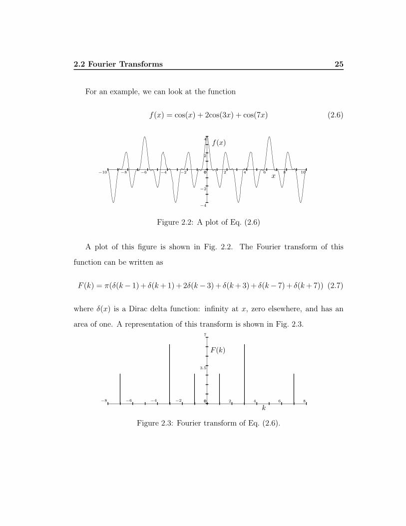
For an example, we can look at the function

f(x) = cos(x) + 2cos(3x) + cos(7x) (2.6)

−10 −8 −6 −4 −2 0 2 4 6 8 10x

−4

−2

0

2

4f(x)

Figure 2.2: A plot of Eq. (2.6)

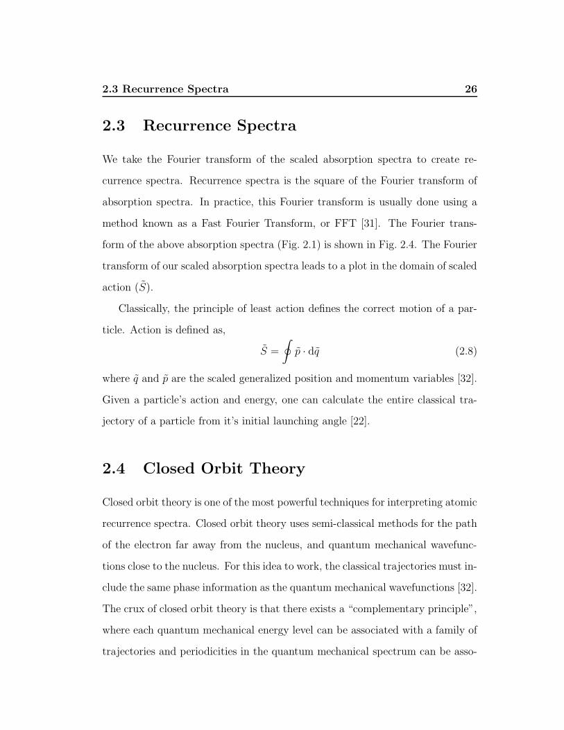
A plot of this figure is shown in Fig. 2.2. The Fourier transform of this

function can be written as

F (k) = π(δ(k− 1)+ δ(k + 1) +2δ(k− 3) + δ(k + 3)+ δ(k− 7) + δ(k + 7)) (2.7)

where δ(x) is a Dirac delta function: infinity at x, zero elsewhere, and has an

area of one. A representation of this transform is shown in Fig. 2.3.

−8 −6 −4 −2 0 2 4 6 8

k0

3.5

7

F (k)

Figure 2.3: Fourier transform of Eq. (2.6).

2.3 Recurrence Spectra 26

2.3 Recurrence Spectra

We take the Fourier transform of the scaled absorption spectra to create re-

currence spectra. Recurrence spectra is the square of the Fourier transform of

absorption spectra. In practice, this Fourier transform is usually done using a

method known as a Fast Fourier Transform, or FFT [31]. The Fourier trans-

form of the above absorption spectra (Fig. 2.1) is shown in Fig. 2.4. The Fourier

transform of our scaled absorption spectra leads to a plot in the domain of scaled

action (S).

Classically, the principle of least action defines the correct motion of a par-

ticle. Action is defined as,

S =

∮

p · dq (2.8)

where q and p are the scaled generalized position and momentum variables [32].

Given a particle’s action and energy, one can calculate the entire classical tra-

jectory of a particle from it’s initial launching angle [22].

2.4 Closed Orbit Theory

Closed orbit theory is one of the most powerful techniques for interpreting atomic

recurrence spectra. Closed orbit theory uses semi-classical methods for the path

of the electron far away from the nucleus, and quantum mechanical wavefunc-

tions close to the nucleus. For this idea to work, the classical trajectories must in-

clude the same phase information as the quantum mechanical wavefunctions [32].

The crux of closed orbit theory is that there exists a “complementary principle”,

where each quantum mechanical energy level can be associated with a family of

trajectories and periodicities in the quantum mechanical spectrum can be asso-

2.4 Closed Orbit Theory 27

PSfrag replacements

Rec

urr

ence

Str

engt

h

Scaled Action0 2 4 6 8 10 12 14

5

5

15

15

25

25

35

35

08/07/97

07/06/97

Figure 2.4: Recurrence spectra of Fig. 2.1 taken by Len Keeler in the Morgan

Lab [32]

ciated with a single closed orbit [30]. Initially, the excited electron is formulated

to be an outgoing wavefront. Away from the nucleus this wavefront is consid-

ered as a set of trajectories. These trajectories form an incoming wavefront that

interferes with the outgoing wavefront to create oscillations in the absorption

spectra [14].

Closed orbit theory originated primarily from work by Delos, Du, and Gao

[12–14, 19–21, 24, 48]. Closed orbit theory has grown into a strong bridge over

the gap between semi-classical and quantum mechanical physics in these highly

excited systems. Taking the Fourier transform of our absorption spectra lets us

assign specific trajectories to lines in the absorption spectra. The Fourier trans-

form illustrates the periodicities in the quantum mechanical structure. These

trajectories can be labeled as ratios of rational numbers, u/v, corresponding to

2.4 Closed Orbit Theory 28

a ratio of angular frequencies of the orbit in parabolic coordinates [16]. This

gives us the ability to relate classical orbital dynamics to the quantum mechan-

ical spectra taken by our apparatus. A more thorough investigation of closed

orbit theory can be found in the doctoral theses of Len Keeler and Heric Flores-

Rueda [16, 32].

Chapter 3

The Portable Rydberg Generator

3.1 Overview of Design

Previous experimentation in the Morgan Lab employed the use of collinear fast-

atom beam technology for conducting laser spectroscopy. Maintaining a 10 keV

particle accelerator for conducting research brings along large and often unnec-

essary headaches. As well, due to the limitations of some of the materials of the

ion source, a finite operating uptime is usually limited to less than one hundred

hours [32].

A new very small apparatus was designed by Len Keeler to fit in an MDC Del-

Seal flange 3 − 3/8′′ six-way cross vacuum chamber. Combined with a diffusion

pump, mechanical pump, and small rack of power supplies, this new apparatus

was designed with the idea that the apparatus could be moved to any available

laser, with laser time being a precious commodity. Because of this notable

quality, the new apparatus was dubbed “The Portable Rydberg Generator”, or

PRG for short (see Fig 3.1 for a schematic diagram and Appendix E for pictures).

3.1 Overview of Design 30

To Vacuum System

?

Gas Handling System

?

Channeltron

�

End-Cup Detector�Stark Plates

6

Electron Source

* Sweepers

�

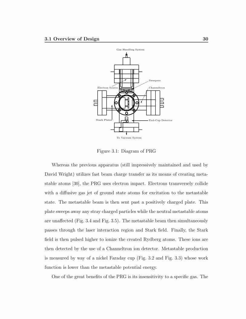
Figure 3.1: Diagram of PRG

Whereas the previous apparatus (still impressively maintained and used by

David Wright) utilizes fast beam charge transfer as its means of creating meta-

stable atoms [30], the PRG uses electron impact. Electrons transversely collide

with a diffusive gas jet of ground state atoms for excitation to the metastable

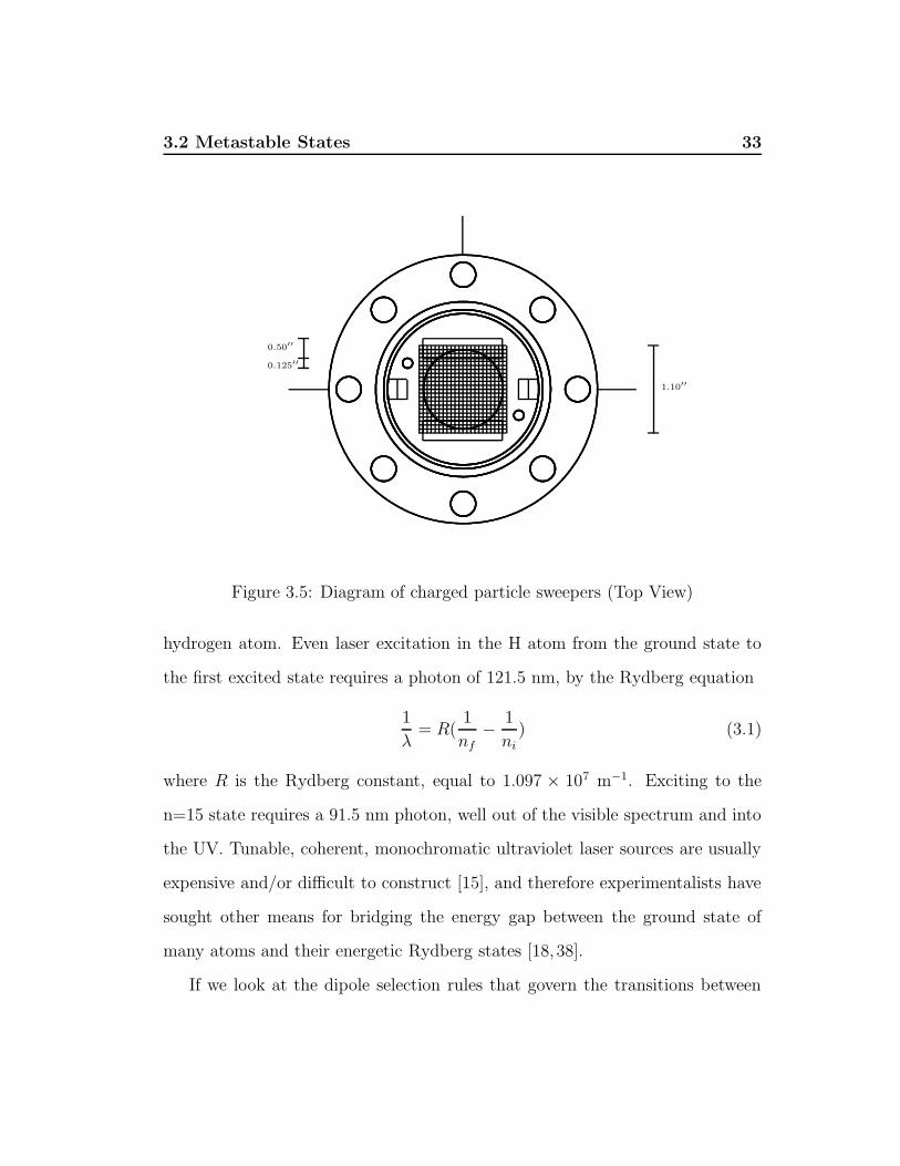
state. The metastable beam is then sent past a positively charged plate. This

plate sweeps away any stray charged particles while the neutral metastable atoms

are unaffected (Fig. 3.4 and Fig. 3.5). The metastable beam then simultaneously

passes through the laser interaction region and Stark field. Finally, the Stark

field is then pulsed higher to ionize the created Rydberg atoms. These ions are

then detected by the use of a Channeltron ion detector. Metastable production

is measured by way of a nickel Faraday cup (Fig. 3.2 and Fig. 3.3) whose work

function is lower than the metastable potential energy.

One of the great benefits of the PRG is its insensitivity to a specific gas. The

3.1 Overview of Design 31

0.75′′

0.25′′

0.125′′

0.20′′

0.375′′

1.25′′

0.25′′ 0.25′′ 1.00′′

0.5′′

0.25′′

Teflon

Nickel

Copper

Cylinder

Figure 3.2: End-cup assembly (Side View)

0.25′′

0.375′′

1.00′′

Figure 3.3: End-cup assembly (Top View)

3.2 Metastable States 32

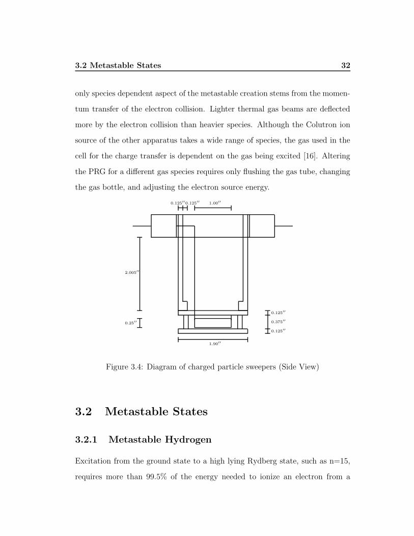
only species dependent aspect of the metastable creation stems from the momen-

tum transfer of the electron collision. Lighter thermal gas beams are deflected

more by the electron collision than heavier species. Although the Colutron ion

source of the other apparatus takes a wide range of species, the gas used in the

cell for the charge transfer is dependent on the gas being excited [16]. Altering

the PRG for a different gas species requires only flushing the gas tube, changing

the gas bottle, and adjusting the electron source energy.

2.005′′

0.125′′

0.375′′

0.125′′

0.125′′0.125′′ 1.00′′

1.90′′

0.25′′

Figure 3.4: Diagram of charged particle sweepers (Side View)

3.2 Metastable States

3.2.1 Metastable Hydrogen

Excitation from the ground state to a high lying Rydberg state, such as n=15,

requires more than 99.5% of the energy needed to ionize an electron from a


1.10′′

0.50′′

0.125′′

Figure 3.5: Diagram of charged particle sweepers (Top View)

hydrogen atom. Even laser excitation in the H atom from the ground state to

the first excited state requires a photon of 121.5 nm, by the Rydberg equation

1

λ= R(

1

nf− 1

ni) (3.1)

where R is the Rydberg constant, equal to 1.097 × 107 m−1. Exciting to the

n=15 state requires a 91.5 nm photon, well out of the visible spectrum and into

the UV. Tunable, coherent, monochromatic ultraviolet laser sources are usually

expensive and/or difficult to construct [15], and therefore experimentalists have

sought other means for bridging the energy gap between the ground state of

many atoms and their energetic Rydberg states [18, 38].

If we look at the dipole selection rules that govern the transitions between


states of a hydrogen atom,

∆m = ±1, 0 (3.2a)

∆l = ±1 (3.2b)

we can generate a diagram of the decay paths of the first four levels of H

(see Fig 3.6). There is no decay route for the hydrogen 2s level to decay to the

ground state via spontaneous emission. This state is known as the metastable

state and is long-lived (∼0.2 seconds for H [23,41]). Excitation from the hydrogen

metastable state to the n=15 state requires a 371.2 nm photon, obtainable by a

dye laser and doubling crystal. Excitation to the metastable state is done by a

variety of means [15,18,32], most notably charge exchange and electron impact.

n = 4

n = 3

n = 2

n = 1

l = 0 l = 1 l = 2 l = 3

� � �j j

� �

�

Rj

�

Figure 3.6: Decay routes by spontaneous emission of the first four energy levels

of hydrogen governed by dipole selection rules.


3.2.2 Multi-Electron Metastable States

As Bethe and Salpeter describe [4], selection rules can be abstracted to any

general atom as

∆m = 0,±1 (3.3a)

∆J = 0,±1 (3.3b)

J = 0 9 J = 0 (3.3c)

where J is the sum of the total system orbital and spin angular momenta. If

the spin-orbit coupling is small (notably for low atomic number) and L and S

are reasonably good quantum numbers, the Russell-Saunders approximation is

valid [10]. In this case, four other selection rules also apply:

∆Ψparity : g → u, u → g (3.4a)

∆L = 0,±1 (3.4b)

L = 0 9 L = 0 (3.4c)

∆S = 0 (3.4d)

Argon has two important metastable states1, 3p54s 3P2 state and 3p54s 3P0

state [5]. Xenon likewise has two notable metastable states, the 5p56s 3P2 state

and the 5p56s 3P0 state [37].

3.2.3 Methods of Metastable Creation

Charge Transfer

One of the more experimentally popular methods for creating metastable atoms

is a method known as charge transfer or electron capture [46]. A beam of accel-

1Denoted 2S+1LJ .


erated ions is sent through a thermal vapor or gas and the ions capture valence

electrons from the vapor (or gas) [11]. Experimental research by Il’in pointed to

much higher efficiencies of electron capture of fast-atoms beams with alkali metal

vapors than gases, by up to a factor of five [28,46]. This experimental work also

confirmed the theoretical research of Oppenheimer [44] and Jackson [29] that

charge transfer from thermal atoms to fast ions populates n-states as 1/n3.

The choice of gas or alkali metal vapor is primarily dependent on two factors,

one practical, one physical. First, the species is experimentally easy to work with;

the substance has a relatively low vaporization temperature, is non-toxic, is non-

reactive, etc. The other criteria is a small energy defect between the species and

the atomic beam excited metastable state [11]. The Morgan Lab has primarily

used sodium and potassium metals for charge transfer [11, 16, 32, 33, 46].

In practice, neutralization rates between forty and fifty percent occur [32].

The neutralization rate can be adjusted by the temperature of the vapor. How-

ever, increasing the vapor temperature increases the number of multiple collision

events. Multiple collisions can directly de-excite a metastable, further excite a

newly created metastable atom to ionization or to a further excited state (quickly

decaying back to the ground state). Using sodium for metastable helium cre-

ation, Len Keeler found up to 75% of created neutrals were in the 23S metastable

state.

Electron Impact

Electron impact has not previously been used for recurrence spectroscopy in the

Morgan Lab. Electron impact is simply colliding a gas with energetic electrons

corresponding to the energy gap of the desired excitation [1]. Therefore, creation

3.3 Electron Sources 37

of metastable states from a ground state gas requires accelerating electrons to

the energy of the metastable state. The electron collides with a gas particle and

the energy transfer excites the ground state electron to the metastable state.

The drawback of this technique is the momentum transfer from the accel-

erated electron inelastically colliding with the gas particle. This effect is small

or even negligible for heavy atoms (such as Ar or Xe) but will heavily deflect

a thermal beam of light atoms [42]. Tommasi et al report a 12◦ deflection for

helium-electron collisions to the 23S1 and 21S0 metastable states [52].

3.3 Electron Sources

3.3.1 HeatWave Labs Source

The original electron source for our apparatus was purchased from HeatWave

Labs, Inc. in Watsonville, California. We purchased a STD 400 TB-198 Standard

Series Barium Tungsten Dispenser Cathode from HeatWave Labs. This source is

reported by the manufacturer to yield 2.5− 4.0 A of electrons with an operating

lifetime greater than ten thousand hours. [25]

-MolyBody

R

Pure AluminaPotting

Emitter Face

-HeaterLead

0.40′′

0.45′′

0.35′′

Figure 3.7: Diagram of HeatWave TB-198 standard series barium tungsten dis-

penser cathode

However, we were unable to obtain lifetimes greater than roughly one hun-

3.4 Operating Parameters 38

dred hours without cathode surface pitting and only marginal electron output.

We also had difficulty fitting these sources into our apparatus without overly

stressing the leads to the source. The high operating temperatures of these

sources, above one thousand degrees Celsius, made it difficult to use any mate-

rials in our apparatus other than stainless steel (which out-gasses impurities at

such high temperatures) and ceramic2. Due to the cost of these electron sources

($562/source) and the difficulty in operating them, we soon looked for other

electron sources.

3.3.2 Southwest Vacuum Devices Source

On the further recommendation from Len Keeler, our lab contacted Southwest

Vacuum Devices. They sell electron guns and emission products, primarily for

televisions and industry. However, their C−14 cathode and related H−61 heaters

suited our needs quite well. Together the cathodes and heaters sell for around

thirteen dollars. Very little concrete documentation on these products was avail-

able from Southwest Vacuum Devices. The cathode is rated to produce around

600 mA off a surface roughly an eighth of an inch in diameter. Unlike the pre-

vious HeatWave Labs electron source, two of these electron sources can be run

in parallel in the PRG.

3.4 Operating Parameters

The first part of getting the PRG operational was investigating whether or not

we can generate metastable atoms. We started with argon gas rather than xenon

2Experimenters take note: Aluminum melts at 660.37◦C [8]


1.060′′0.625′′

0.25′′

0.125′′

0.375′′

0.684′′

0.188′′

0.22′′

1.060′′

0.19′′0.116′′

0.0825′′ 0.0825′′0.375′′ 0.375′′0.145′′

0.062′′

0.10′′

0.10′′

0.55′′

0.094′′

0.562′′

0.094′′

0.10′′ 0.325′′

0.094′′ 0.094′′0.872′′

0.125′′

0.188′′ 0.188′′

0.188′′

0.188′′

0.684′′

0.374′′

0.52′′

0.50′′ 0.375′′

0.52′′

0.375′′

Figure 3.8: PRG electron source (Side and Exploded Top View) (SW-Vacuum

Device Configuration)


0.50′′

0.125′′ 0.10′′

0.075′′0.125′′ 0.70′′

Figure 3.9: Southwest Vacuum Devices C−14 cathode diagram

for our initial experiments. Recent experimental argon data by David Wright on

the other apparatus in the Morgan Lab gave us experimental data to check our

results to. Xenon is also more expensive compared to argon. We first biased our

nickel end-cup by 27 V using three 9 V batteries. After warming up our electron

sources and letting them stabilize, we measured the current from the end-cup

as we increased the electron energy from eight to twenty-four electron-volts.

Nickel has a low electron work function of 5.15 eV [8]. Colliding the nickel with

energetic neutral thermal atoms generates a current in the nickel from secondary

electron emission that can be measured with a picoammeter.

We first measured the background signal by measuring the end-cup current

with no argon gas in the system, a background pressure around 2×10−7 torr, and

the sweepers off for electron accelerations between eight and twenty-four volts.

This negative background signal therefore stems from stray electrons from the

electron source and other errant charged particles in the apparatus. Next, a po-

tential of approximately one hundred and forty volts was placed on the sweepers

to keep stray electrons from reaching the end-cup and the end-cup current was

once again measured for electron acceleration voltages of eight to twenty-four

volts. Argon gas was next introduced into the system to a total pressure of

4.2×10−6 torr. The current from the end-cup was once again measured for elec-

tron acceleration voltages between eight and twenty-four volts with the sweepers


PSfrag

replacem

ents

V

A = 0.00030625V 2− 0.0038195V + 0.0049097

A

6

8 10 12 14 16 18 20 22 24

0

0.12

0.1

0.08

0.06

0.04

0.02

−0.02

Figure 3.10: Electron source output current (A) of Southwest Vacuum Devices

source as a function of acceleration voltage (V). Electron Source heaters were at

12 V , drawing ∼2 A.

off and then on. Argon has a metastable energy of 11.55 eV [43] and an ion-

ization energy of 15.76 eV [53]. Therefore, we should start to see metastable

atoms being made just at 11.55 eV , with the metastable production increasing

until ionization takes over past 15.76 eV . This data was then analyzed to see if

metastable argon atoms were being produced.

Chapter 4

Experimental Data and Analysis

PSfrag

replacem

ents

V

A

6 8 10 12 14 16 18 20 22 24

0

No SweepersSweepers

2 × 10−11

−2 × 10−11

−4 × 10−11

−6 × 10−11

−8 × 10−11

−1 × 10−10

−1.2 × 10−10

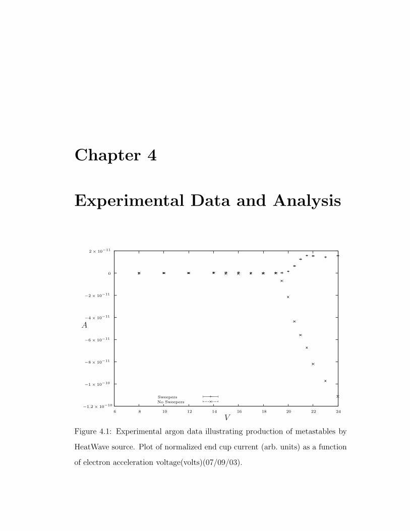
Figure 4.1: Experimental argon data illustrating production of metastables by

HeatWave source. Plot of normalized end cup current (arb. units) as a function

of electron acceleration voltage(volts)(07/09/03).


PSfrag

replacem

ents

A

V

6

8 10 12 14 16 18 20 22 24

0

−2 × 10−10

2 × 10−10

−4 × 10−10

4 × 10−10

−6 × 10−10

6 × 10−10

−8 × 10−10

8 × 10−10

1 × 10−9

1.2 × 10−9

No Sweepers

Sweepers

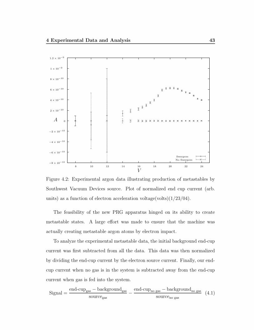
Figure 4.2: Experimental argon data illustrating production of metastables by

Southwest Vacuum Devices source. Plot of normalized end cup current (arb.

units) as a function of electron acceleration voltage(volts)(1/23/04).

The feasibility of the new PRG apparatus hinged on its ability to create

metastable states. A large effort was made to ensure that the machine was

actually creating metastable argon atoms by electron impact.

To analyze the experimental metastable data, the initial background end-cup

current was first subtracted from all the data. This data was then normalized

by dividing the end-cup current by the electron source current. Finally, our end-

cup current when no gas is in the system is subtracted away from the end-cup

current when gas is fed into the system.

Signal =end-cupgas − backgroundgas

sourcegas

−end-cupno gas − backgroundno gas

sourceno gas

(4.1)


PSfrag

replacem

ents

A

V

SW Vacuum Devices

HeatWave Inc.

6 8 10 12 14 16 18 20 22 24

0

−2 × 10−10

2 × 10−10

−4 × 10−10

4 × 10−10

−6 × 10−10

6 × 10−10

8 × 10−10

Figure 4.3: Comparison of experimental argon metastable data from Fig. 4.1

and Fig. 4.2.

Plots of the normalized signal vs electron acceleration voltage can be seen in

Fig. 4.1 (HeatWave source) and Fig. 4.2 (Southwest Vacuum Devices source).

The points in these plots are of experimentally measured data, while the error

bars in these plots are the range given by the precision of our measurement

devices. This signal represents excitation to both the 3P0 and 3P2 metastable

states of argon.

Although the Southwest Vacuum Devices sources produces a much smaller

electron current than the HeatWave electron sources, the Southwest Vacuum

Devices source is much more efficient in its metastable production. The normal-

ized, sweepers on, end-cup current from the two sources is compared in Fig. 4.3.


PSfrag

replacem

ents

V

A

12 14 16 18 20 22 24

0

1

2

3

4

5

Experiment

Theory

Figure 4.4: Comparison of experimental argon data and known apparent electron

impact excitation cross sections (arb. units) as a function of electron energy

(volts). Cross section data taken from [6, 45].

This efficiency is not terribly surprising, as that the surface area of the HeatWave

source is much larger than the atomic beam path area. Therefore, most of the

electrons from the HeatWave electron gun never interact with a gas atom.

On comparison of our experiment data with other experimental data [6] and

theoretical analysis [7, 45], as shown in Fig. 4.4, we can conclude that argon

metastable atoms are successfully being created by our apparatus.

Chapter 5

Conclusion and Future Work

Our lab has not yet successfully taken absorption spectra with our new appara-

tus. However, we have certainly seen the feasibility of using electron impact as

a method for creating metastable atoms.

Difficulties in obtaining absorption spectra from the new apparatus come

from an overwhelming background absorption signal on our Channeltron detec-

tor. The laser beam seems to not only excite our desired beam of atoms, but

background gas as well, even at Ultra-High Vacuum pressures. In our previous

experiments we have been able to steer our fast-atom beam towards our ion de-

tector with electric fields [32]. This method has let us separate our excited beam

from our excited background noise. However, our thermal beam passes directly

in front of our Channeltron detector and cannot be easily separated from the

background signal. We continue to search for a clean absorption signal from the

Portable Rydberg Generator.

As stated earlier, our eventual goal is to take scaled recurrence spectra of

Rydberg xenon in Stark fields. An interesting area of investigation may be

5 Conclusion and Future Work 47

utilizing the electron impact source with the particle accelerator used in previous

experiments in the Morgan Lab. After investigating xenon, our lab looks to begin

research into scaled recurrence spectroscopy of Rydberg molecular hydrogen. As

Professor Tom Morgan likes to tell his lab group, “The future is molecules!”

Appendix A

Stark Frequency Derivation

This derivation comes from Hezel et al [27], but is included for completeness.

We can first begin with Hamilton’s equations:

~p = − ~∇rH (A.1a)

~r = ~∇pH (A.1b)

for the Hamiltonian,

H = HCoulomb + V (~r) (A.2)

From this we can generate the change in momentum as

~p = ~pc − ~∇V (~r) (A.3)

By manipulating the definition of angular momentum,

~L = ~r × ~p, (A.4)

to find the change in angular momentum,

~L = ~r × ~p + ~r × ~p (A.5)


Substituting our Hamiltonian into Eq. (A.5) and noting that

~Lc = 0 (A.6)

we find

~L = −~r × ~∇V (~r) (A.7)

The gradient of potential is the electric field, ~F . Eq. (A.7) can therefore be

rewritten as

~L = −~r × ~F (A.8)

The change in angular momentum is torque, written as,

~L = ~τ (A.9)

Due to the rapid motion of the electron,

< r >= − < d > (A.10)

Note that by applying Eq. (A.9) and Eq. (A.10) to Eq. (A.8) yields the expression

for the torque of a dipole,

~τ = ~d × ~F (A.11)

From Eq. (1.25), the average distance can be written as

< d >=3

2n2 ~A = − < r > (A.12)

This makes our change in angular momentum

~L =3

2n2( ~A × ~F ) (A.13)

Setting ~F = Fz makes Lz = 0. Lz is therefore a conserved quantity and usable

as a commuting operator for the Stark effect in parabolic coordinates.


We can derive a similar expression for ~A in the following manner. Taking the

derivative of the definition of ~A leads to

~A = ~p × ~L + ~p × ~L − ˙r (A.14)

We can substitute Eq. (A.3) for ~p,

~A = ( ~pc − ~∇V (~r)) × ~L + ~p × ~L − ˙r (A.15)

~A = ( ~pc × ~L − ˙r) − ~F × ~L + ~p × ~L (A.16)

We can refer to the Coulombic Runge-Lenz vector as

~Ac = ~pc × ~L − ˙r (A.17)

For a 1/~r potential, ~Ac = 0. Therefore,

~A = −~F × ~L + ~p × ~L (A.18)

By applying Eq. (A.8) to ~p × ~L, we can write

~p × ~L = ~p × (−~r × ~F ) (A.19)

Using the ”BAC-CAB” rule for triple cross products,

~A × ( ~B × ~C) = ~B · ( ~A · ~C) − ~C · ( ~A · ~B) (A.20)

We can now write Eq. (A.19) as

~p × ~L = F (~p · ~r) − ~r(~p · ~F ) (A.21)

We now look to evaluate the time average of these two above terms.

~p · ~r =d~r

dt· ~r =

1

2

d

dt(~r)2 (A.22)


The average over a whole period of an exact differential of a periodic function is

zero, so Eq. (A.22) = 0. Thus,

~p × ~L = −~r(~p · ~F ) (A.23)

This makes Eq. (A.18) become

~A = −~F × ~L − ~r(~p · ~F ) (A.24)

If we inspect the product ~F × ~L,

~F × ~L = ~F × (~r × ~p) (A.25)

which by the ”BAC-CAB”, Eq. (A.20), rule can be written as,

~F × ~L = ~r(~F · ~p) − ~p(~F · ~r) (A.26)

This quantity can be shown to be equal to the negative derivative of ~r(~r · ~F ),

~r(~F · ~p) − ~p(~F · ~r) = − d

dt~r(~r · ~F ) (A.27)

This exact differential also averages to zero. Therefore,

< ~r(~F · ~p) >= − < ~p( ~F · ~r) > (A.28)

If we substitute this into Eq. (A.26) we have the expression

~F × ~L = − < 2~p(~F · ~r) > (A.29)

Finally applying this to Eq. (A.24) leads to an equation for ~A:

~A =3

2(~L × ~F ) (A.30)


Eqs. (A.13) and (A.30) can be uncoupled and evaluated by differentiating

one and substituting into the other equation. Differentiation of Eq. (A.30) yields

the equation

~A =3

2((~L × ~F ) + ( ~F × ~L)) (A.31)

Since we are investigating static fields, we can drop the second term from

Eq. (A.31). Substituting Eq. (A.13) into Eq. (A.31) leads to

~A =3

2n2(( ~A × ~F ) × ~F ) (A.32)

Applying the fact that

~A × ~B = −( ~B × ~A) (A.33)

and the “BAC-CAB” rule, Eq. (A.20), we can then write

~A = −(3

2n)2( ~A(~F · ~F ) − ~F (~F · ~A)) (A.34)

If ~F = Fz then we have the set of equations

Ax = −(3

2)2n2F 2Ax (A.35a)

Ay = −(3

2)2n2F 2Ay (A.35b)

Az = 0 (A.35c)

These second-order differential equations can be solved by an equation of the

form

A(t) = Cei( 32nFt) (A.36)

Setting our amplitudes as Ax0 and Ay0, respectively, and Ay(t = 0) = 0, gener-

ates the equation:

Ax(t)2 + Ay(t)

2 = A2x0cos2(ωst) + A2

y0sin2(ωst) (A.37)

where ωs = 3/2nF , the Stark frequency. A similar treatment of ~L leads to an

equation analogous to Eq. (A.37).

Appendix B

Hamiltonian Scaling Derivation

This derivation is thanks to [32]. Our Coulombic Hamiltonian is the familiar

H =p2

2− 1

r(B.1)

We can add a Stark field term in the z-direction to our Hamiltonian,

H =p2

2− 1

r+ Fz (B.2)

We now look to scale our position, r, and momentum, p, so that our Hamiltonian

is independent of the applied Stark field. We can define our scaled variables as

r = F αr (B.3a)

p = F βp (B.3b)

Our scaled Hamiltonian therefore becomes,

H = F 2β p2

2− F−α 1

r+ F α+1z (B.4)

Each term in our scaled Hamiltonian must have the same field dependence.

Thus,

2β = −α = α + 1 (B.5)

B Hamiltonian Scaling Derivation 54

We can solve for α and β to be

α = −1

2(B.6a)

β =1

4(B.6b)

We now have the scaling parameters:

r = F−1/2r (B.7a)

p = F 1/4p (B.7b)

When these scaling variable are substituted into our Hamiltonian, Eq. (B.2),

we can develop a scaled Hamiltonian relationship,

H = F 1/2 p2

2− F 1/2 1

r+ F (F−1/2)z (B.8)

H = HF−1/2 (B.9)

We can referred to the scaled energy of our scaled Hamiltonian as ε. From

Eq. (B.9) leads the scaled energy relation

ε =E√F

(B.10)

Our scaled Hamiltonian is now completely independent of the external field.

Appendix C

Southwest Vacuum Devices

Cathode Installation

1. Place C−14 cathodes in cathode holder.

2. Using resistance welder, weld cathode leads onto cathode holder body.

3. For each source, weld one heater lead to cathode lead.

4. Weld nickel wire between un-welded heater leads(1)1.

5. Weld nickel wire between cathode leads (2).

6. Assemble cathode holder together with base and extraction grid.

7. Weld external leads to nickel wire (1) and nickel wire (2) using nickel wire.

8. Install sweeper assembly onto source.

1To keep from confusion about heater leads, each heater has two leads. One lead of a heater

shall be denoted (1), the other (2). The two heaters are wired in parallel.

C Southwest Vacuum Devices Cathode Installation 56

9. Install source into vacuum chamber.

10. Pump chamber below 10−7 torr.

11. Check for electrical shorting between cathode and case, as well as continu-

ity on cathode leads.

12. Apply 7.5 V to the cathode for three minutes.

13. Apply 12.5 V to the cathode for two minutes.

14. Apply 10 V to the cathode for thirty minutes. Put 125 V - 150 V bias on

the cathode during this step.

15. Lower cathode voltage to ∼4 V and purge gas valve at a pressure no higher

than 5 × 10−5 torr.

16. Run source at ∼9 V. Heaters should draw roughly 2.0 A.

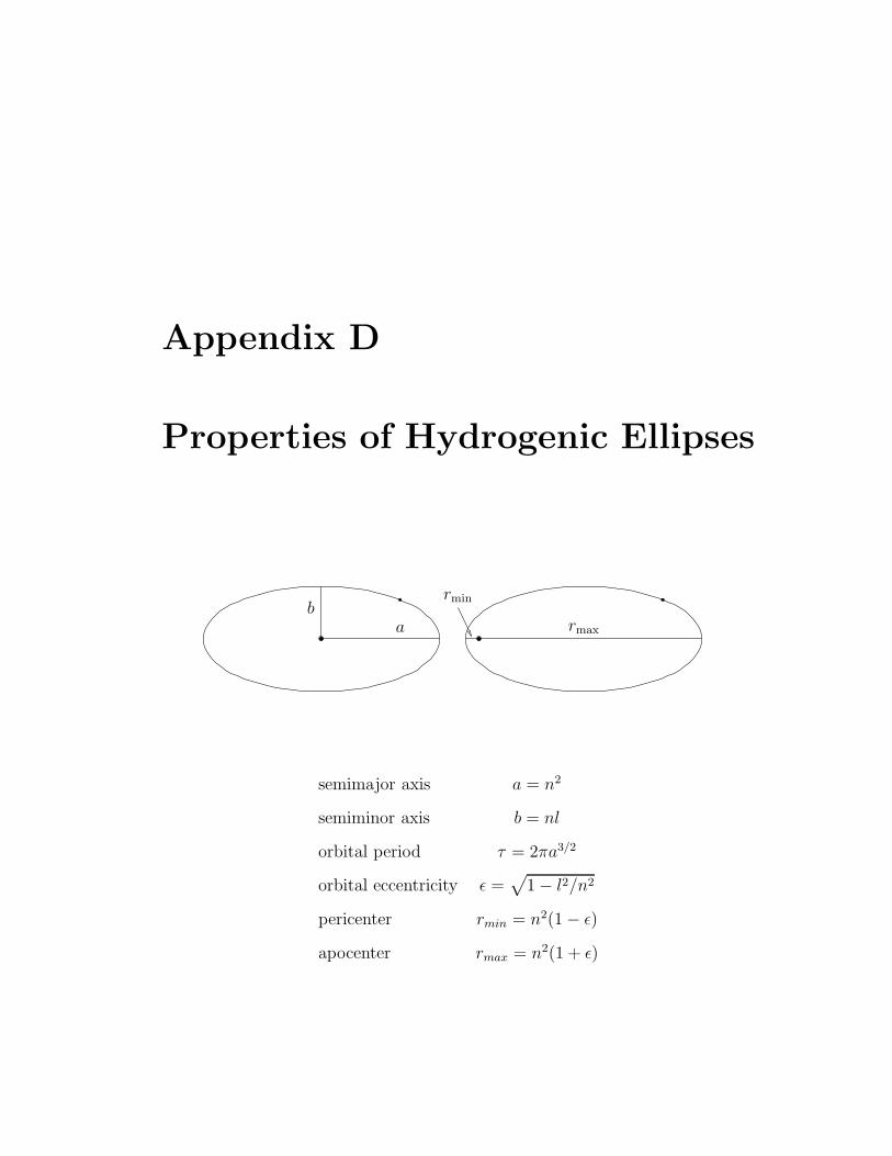
Appendix D

Properties of Hydrogenic Ellipses

ab

rmax

rmin

semimajor axis a = n2

semiminor axis b = nl

orbital period τ = 2πa3/2

orbital eccentricity ε =√

1 − l2/n2

pericenter rmin = n2(1 − ε)

apocenter rmax = n2(1 + ε)

Appendix E

Pictures of the Portable Rydberg

Generator

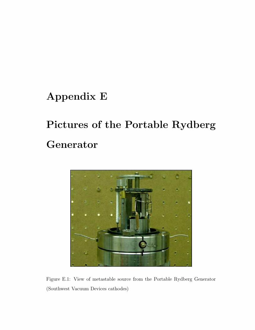
Figure E.1: View of metastable source from the Portable Rydberg Generator

(Southwest Vacuum Devices cathodes)


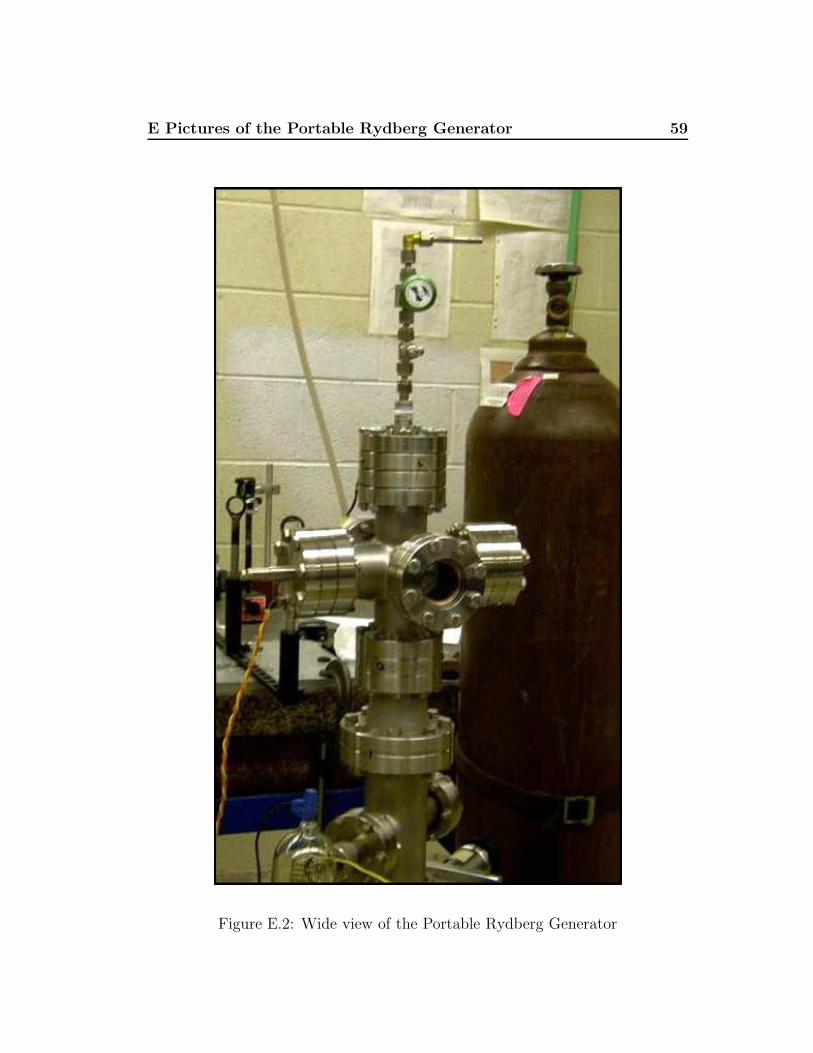
Figure E.2: Wide view of the Portable Rydberg Generator


Figure E.3: Side view of the Portable Rydberg Generator

Bibliography

[1] N. Andersen, J. W. Gallagher, and I. V. Hertel. Collisional alignment and

orientation of atomic outer shells: I. direct excitation by electron and atom

impact. Physics Reports, 165:1, 1988.

[2] J. F. Baugh, D. A. Edmonds, P. T. Nellesen, C. E. Burkhardt, and J. J. Lev-

enthal. Coherent states composed of Stark eigenfunctions of the hydrogen

atom. Am. J. Phys., 65:1097, 1997.

[3] R. J. Bell. Introductory Fourier Transform Spectroscopy. Academic Press,

1972.

[4] H. Bethe and E. Salpeter. Quantum Mechanics of One- and Two-Electron

Systems. Plenum Publishing, 1977.

[5] J. B. Boffard, G. A. Piech, M. F. Gehrke, M. E. Lagus, L. W. Anderson,

and C. C. Lin. Electron impact excitation out of the metastable levels of

argon into the 3p54p J = 3 level. J. Phys. B: At. Mol. Opt. Phys., 29:L795,

1996.

[6] W. L. Borst. Excitation of metastable argon and helium atoms by electron

impact. Phys. Rev. Lett., 9:1195, 1974.

Bibliography 62

[7] J. Bretagne, G. Delouya, J. Godart, and V. Puech. High-energy electron

distribution in an electron-beam-generated argon plasma. J. Phys. D: Appl.

Phys., 14:1225, 1981.

[8] Chemical Rubber Company. CRC standard mathematical tables and formu-

lae. CRC Press, 1991.

[9] T. Clausen. Quantum Chaos in the periodically driven Hydrogen Atom. PhD

thesis, Wesleyan University, 2002.

[10] E. U. Condon and G. H. Shortley. The Theory of Atomic Spectra. Cambridge

University Press, 1959.

[11] D. Cullinan. Electric field effects on helium Rydberg atoms. Master’s thesis,

Wesleyan University, 1997.

[12] J. B. Delos, R. L. Waterland, and M. L. Du. Semiclassical interpretation

of eigenvectors for excited atoms in external fields. Phys. Rev. A, 37:1185,

1988.

[13] M. L. Du and J. B. Delos. Effect of closed classical orbits on quantum

spectra: Ionization of atoms in a magnetic field, I. physical picture and

calculations. Phys. Rev. A, 38:1896, 1988.

[14] M. L. Du and J. B. Delos. Effect of closed classical orbits on quantum

spectra: Ionization of atoms in a magnetic field. II. derivation of formulas.

Phys. Rev. A, 38:1913, 1988.

Bibliography 63

[15] W. E. Ernst, T. P. Softley, and R. N. Zare. Stark-effect studies in xenon au-

toionizing Rydberg states using a tunable extreme-ultraviolet laser source.

Phys. Rev. A, 37:4172, 1988.

[16] H. Flores-Rueda. Stark Recurrence Spectroscopy of Rydberg Helium and

Argon Atoms: The Covergence of Quantum and Classical Mechanics. PhD

thesis, Wesleyan University, 2002.

[17] A. P. French. Vibrations and Waves. W. W. Norton & Company, 1971.

[18] T. Gallagher. Rydberg Atoms. Cambridge University Press, 1994.

[19] J. Gao and J. B. Delos. Closed-orbit theory of oscillations in atomic pho-

toabsorption cross sections in a strong electric field. II. derivation of formu-

las. Phys. Rev. A, 46:1455, 1992.

[20] J. Gao and J. B. Delos. Resonances and recurrences in the absorption

spectrum of an atom in an electric field. Phys. Rev. A, 49:869, 1994.

[21] J. Gao, J. B. Delos, and M. Baruch. Closed-orbit theory of oscillations

in atomic photoabsorption cross sections in a strong electric field. I. com-

parison between theory and experiments on hydrogen and sodium above

threshold. Phys. Rev. A, 46:1449, 1992.

[22] H. Goldstein. Classical Mechanics. Addison-Wesley, 1980.

[23] D. Griffiths. Introduction of Quantum Mechanics. Prentice Hall, Inc., 1995.

[24] M. R. Haggerty and J. B. Delos. Recurrence spectroscopy in time-dependent

fields. Phys. Rev. A, 61:053406, 2000.

Bibliography 64

[25] HeatWave Labs, Inc. TB-198 Standard Series Barium Tungsten Dispenser

Cathodes. http://www.cathode.com/, 2002.

[26] T. P. Hezel, C. E. Burkhardt, M. Ciocca, L.-W. He, and J. J. Leventhal.

Classical view of the properties of Rydberg atoms: Application of the cor-

respondence principle. Am. J. Phys., 60:329, 1992.

[27] T. P. Hezel, C. E. Burkhardt, M. Ciocca, and J. J. Leventhal. Classical

view of the Stark effect in hydrogen atoms. Am. J. Phys., 60:324, 1991.

[28] R. N. Il’in, B. I. Kikiani, V. A. Oparin, E. S. Solov’ev, and N. V. Fedorenko.

Formation of highly excited hydrogen atoms by proton charge exchange in

gases. Sov. Phys. - JETP, 20:835, 1965.

[29] J. D. Jackson and H. Schiff. Electron capture by protons passing through

hydrogen. Phys. Rev., 89:359, 1953.

[30] R. V. Jensen, H. Flores-Rueda, J. D. Wright, M. L. Keeler, and T. J. Mor-

gan. Structure of the Stark recurrence spectrum. Phys. Rev. A, 62:053410,

2000.

[31] J. Kauppinen and J. Partanen. Fourier Transforms in Spectroscopy. Wiley-

Vch, 2001.

[32] M. L. Keeler. The Recurrence Spectroscopy of Helium. PhD thesis, Wesleyan

University, 1998.

[33] M. L. Keeler, H. Flores-Rueda, J. D. Wright, and T. J. Morgan. Scaled-

energy spectroscopy of argon atoms in an electric field. J. Phys. B, 37:809,

2004.

Bibliography 65

[34] M. L. Keeler and T. J. Morgan. Scaled-energy spectroscopy of the Rydberg-

Stark spectrum of helium: Influence of exchange on recurrence spectra.

Phys. Rev. Lett., 80:5726, 1998.

[35] M. L. Keeler and T. J. Morgan. Core-scattered combination orbits in the

m = 0 Stark spectrum of helium. Phys. Rev. A, 59:4559, 1999.

[36] M. L. Keeler and T. J. Morgan. Behavior of non-classical recurrence am-

plitudes near closed orbit bifurcations in atoms. Phys. Rev. A, 69:012103,

2004.

[37] R. D. Knight and L. Wang. One-photon laser spectroscopy of the np and

nf Rydberg series in xenon. J. Opt. Soc. Am. B, 2:1084, 1985.

[38] R. D. Knight and L. Wang. Stark structure in Rydberg states of xenon.

Phys. Rev. A, 32:896, 1985.

[39] P. Labastie, F. Biraben, and E. Giacobino. Optogalvanic spectroscopy of

the ns and nd Rydberg states of xenon. J. Phys. B: At. Mol. Phys., 15:2595,

1982.

[40] L. D. Landau and E. M. Lifshitz. Mechanics. Butterworth-Heinemann,

1976.

[41] M. Mizushima. Quantum Mechanics of Atomic Spectra and Atomic Struc-

ture. W.A. Benjamin, 1970.

[42] A. J. Murray and P. Hammond. Laser probing of metastable atoms and

molecules deflected by electron impact. Phys. Rev. Lett., 82:4799, 1999.

Bibliography 66

[43] National Institute of Standards and Technology. NIST Atomic

Spectra Database Levels Data Ar I. http://physics.nist.gov/cgi-

bin/AtData/display.ksh?XXE1qArqIXXT2XXI, 2004.

[44] J. R. Oppenheimer. On the quantum theory of the capture of electrons.

Phys. Rev., 31:349, 1928.

[45] V. Puech and L. Torchin. Collision cross sections and electron swarm pa-

rameters in argon. J. Phys. D: Appl. Phys., 19:2309, 1986.

[46] S. P. Renwick. Quasi-Free Scattering in the Ionization and Destruction

of Hydrogen and Helium Rydberg Atoms in Collision with Neutral Targets.

PhD thesis, Wesleyan University, 1991.

[47] J. R. Rubbmark, M. M. Kash, M. G. Littman, and D. Kleppner. Dynamical

effects at avoided level crossing: A study of the Landau-Zener effect using

Rydberg atoms. Phys. Rev. A, 23:3107, 1981.

[48] J. A. Shaw, J. B. Delos, M. Courtney, and D. Kleppner. Recurrences asso-

ciated with a classical orbit in the node of a quantum wave function. Phys.

Rev. A, 52:3695, 1995.

[49] H. J. Silverstone. Perturbation theory of the Stark effect in hydrogen to

arbitrarily high order. Phys. Rev. A, 18:1853, 1978.

[50] R. F. Stebbings and F. B. Dunning. Rydberg states of atoms and molecules.

Cambridge University Press, 1983.

[51] R. F. Stebbings, C. J. Latimer, W. P. West, F. B. Dunning, and T. B. Cook.

Studies of xenon atoms in high Rydberg states. Phys. Rev. A, 12:1453, 1975.

Bibliography 67

[52] O. Tommasi, G. Bertuccelli, M. Francesconi, F. Giammanco, D. Romanini,

and F. Strumia. A high-density collimated metastable he beam with pop-

ulation inversion. J. Phys. D: Appl. Phys., 25:1408, 1992.

[53] I. Velchev, W. Hogervorst, and W. Ubachs. Precision VUV spectroscopy of

Ar I at 105 nm. J. Phys. B: At. Mol. Opt. Phys., 32:L511, 1999.

[54] L. Wang and R. D. Knight. Two-photon laser spectroscopy of the ns′ and

nd′ autoionizing Rydberg series in xenon. Phys. Rev. A, 34:3902, 1986.

[55] J. B. M. Warntjes, C. Nicole, F. Rosca-Pruna, I. Sluimer, and M. J. J.

Vrakking. Two-channel competition of autoionizing Rydberg states in an

electric field. Phys. Rev. A, 63:053403, 2001.

[56] W. P. West, G. W. Foltz, F. B. Dunning, C. J. Latimer, and R. F. Stebbings.

Absolute measurements of collisional ionization of xenon atoms in well-

defined high Rydberg states. Phys. Rev. Lett., 36:854, 1975.

[57] M. L. Zimmerman, M. G. Littman, M. M. Kash, and D. Kleppner. Stark

structure of the Rydberg states of alkali-metal atoms. Phys. Rev. A, 20:2251,

1979.

Index

action, 26

principle of least action, 26

aluminum, 38

angular momentum, 10, 11, 15, 48

argon, 1, 20, 37, 38, 40, 41, 43, 45

atomic units, 12

avoided crossings, 20

Bethe, H., 17, 35

Bohr, N., 9, 10

Bohr model, 9, 16

Channeltron, 30, 46

charge transfer, 30, 32, 34–36

closed orbit theory, 20, 26–28

Colutron, 32

Coulomb potential, 8, 11, 13, 15, 16,

19

de Broglie

formula, 10

wavelength, 10

Delos, J. B., 27

dipole

energy, 14

moment, 11, 13

selection rules, 33, 34

torque, 49

Dirac delta function, 25

Du, M. L., 27

Dunning, F. B., 20

electric quantum number, 17

electron orbital radius, 10

electron impact, 30, 32, 34, 36, 43,

45–47

electron orbital radius, 10

ellipse, 13, 15

apocenter, 57

eccentricity, 13, 14, 57

focus, 13

orbit, 13

orbital period, 57

pericenter, 13, 57

Index 69

precession, 15

semimajor axis, 15, 57

semiminor axis, 15, 57

end-cup, 30, 31, 40, 43, 44

energy defect, 36

Ernst, W. E., 20

fast-atom beam, 29, 30, 36, 46

Flores-Rueda, H., 28

Fourier transform, 24–27

FFT, 26

Gao, J., 27

Hamilton’s equations, 14, 48

Hamiltonian, 17, 22, 23, 48, 49, 53,

54

HeatWave Labs, 37, 38, 42, 44, 45

helium, 20, 36, 37

Hezel, T. P., 14, 17, 48

hydrogen, 9, 11, 13–17, 19, 33, 34

molecular, 47

zero field, 16

Il’in, R. N., 36

Jackson, J. D., 36

Keeler, M. L., 22, 24, 27–29, 36, 38

Keplerian orbit, 9–11

Knight, R. D., 20

Landau, L. D., 13

Lifshitz, E. M., 13

MDC, 29

metastable, 1, 30, 32, 34–38, 41–46

Morgan, T. J., 47

Morgan Lab, 1, 20, 24, 27, 29,

36, 47

Nd:YAG laser, 23

nickel, 40, 55

work function, 40

Oppenheimer, J. R., 36

parabolic coordinates, 17, 18, 20, 28,

49

perturbation theory, 18

first order, 18, 19

second order, 18, 19

polar coordinates, 11

potassium, 36

PRG, 1, 29, 30, 32, 38, 39, 43, 58–60

quantum chaos, 8

quantum defect, 20

Index 70

Runge-Lenz vector, 13, 14, 17, 50

Russell-Saunders approximation, 35

Rydberg atom, 1, 8, 9, 20, 21, 30, 32,

33, 46

Rydberg formula, 11, 12, 19, 33

Salpeter, E., 17, 35

scaled action, 26

scaled energy, 23, 24, 54

scaling variables, 23

Schrodinger equation, 16

Silverstone, H. J., 18

sodium, 21, 36

Softley, T. P., 20

Southwest Vacuum Devices, 38–41,

43, 44, 58

spectroscopy, 23

absorption, 21–24, 26, 27, 46

laser, 29

optogalvanic, 21

recurrence, 1, 8, 21, 22, 26, 27,

36, 47

spherical coordinates, 16, 17

spin-orbit coupling, 35

spontaneous emission, 34

Stark

field, 1, 8, 9, 11, 15, 17, 21, 30,

46, 49, 53

frequency, 15, 52

shift, 19

Stebbings, R. F., 20

sweepers, 30, 32, 33, 40, 44

Tommasi, O., 37

Wang, Liang-guo, 20

Warntjes, J. B. M., 21

Wright, J. D., 30

xenon, 20, 21, 35, 37, 38, 40, 46, 47

Zare, R. N., 20

Date post:	04-Apr-2018
Category:	Documents
Upload:	votruc
View:	229 times
Download:	1 times

Metastable Argon Atoms and the Portable … Argon Atoms and the Portable Rydberg Generator: ......

Documents