1 Metastable Walking Machines Katie Byl, Member, IEEE and Russ Tedrake, Member, IEEE Abstract— Legged robots that operate in the real world are inherently subject to stochasticity in their dynamics and uncer- tainty about the terrain. Due to limited energy budgets and limited control authority, these “disturbances” cannot always be canceled out with high-gain feedback. Minimally-actuated walking machines subject to stochastic disturbances no longer satisfy strict conditions for limit-cycle stability; however, they can still demonstrate impressively long-living periods of continuous walking. Here, we employ tools from stochastic processes to examine the “stochastic stability” of idealized rimless-wheel and compass-gait walking on randomly generated uneven terrain. Furthermore, we employ tools from numerical stochastic optimal control to design a controller for an actuated compass gait model which maximizes a measure of stochastic stability - the mean first-passage-time - and compare its performance to a deterministic counterpart. Our results demonstrate that walking is well-characterized as a metastable process, and that the stochastic dynamics of walking should be accounted for during control design in order to improve the stability of our machines. I. I NTRODUCTION The dynamics of legged locomotion are plagued with com- plexity: intermittent ground interactions, variations in terrain and external perturbations all have a significant (and stochas- tic) impact on the evolution of dynamics and ultimate stability of both animals and machines which walk. Detailed analytical and computational investigations of simplified models have captured much that is fundamental in the dynamics of walking (Coleman, Chatterjee, & Ruina, 1997; Garcia, Chatterjee, Ruina, & Coleman, 1998; Goswami, Thuilot, & Espiau, 1996; Koditschek & Buehler, 1991; McGeer, 1990). These analyses reveal the limit cycle nature of ideal walking systems and often employ Poincar´ e map analysis to assess the stability of these limit cycles. However, the very simplifications which have made these models tractable for analysis can limit their utility. Experimental analyses of real machines based on these simple models (Collins, Ruina, Tedrake, & Wisse, 2005) reveal that the real devices differ from their idealized dynamics in a number of important ways. Certainly the dynamics of impact and contact with the ground are more subtle than what is cap- tured by the idealized models. But perhaps more fundamental is the inevitable stochasticity in the real systems. More than just measurement noise, robots that walk are inherently prone to the stochastic influences of their environment by interacting with terrain which varies at each footstep. Even in a carefully designed laboratory setting, and especially for passive and minimally-actuated walking machines, this stochasticity can have a major effect on the long-term system dynamics. In practice, it is very difficult (and technically incorrect) to apply deterministic limit cycle stability analyses to our experimental walking machines - the real machines do not have true limit cycle dynamics. In this paper, we extend the analysis of simplified walking models toward real machines by adding stochasticity into our models and applying mathematical tools from stochastic analysis to quantify and optimize stability. We examine two classic models of walking: the rimless wheel (RW) and the compass gait (CG) biped. Although we have considered a number of sources of uncertainty, we will focus here on a compact and demonstrative model - where the geometry of the ground is drawn from a random distribution. Even with mild deviations in terrain from a nominal slope angle, the resulting trajectories of the machine are different on every step, and for many noise distributions (e.g., Gaussian) the robot is guaranteed to eventually fall down (with probability one as t →∞). However, one can still meaningfully quantify stochastic stability in terms of expected time to failure, and maximization of this metric in turn provides a principled approach to controller design for walking on moderately rough, unmodeled terrain. Stochastic optimization of a controlled compass gait model on rough terrain reveals some important results. Modeling walking as a metastable limit cycle changes the optimal control policy; upcoming terrain knowledge, or knowledge of the terrain distribution, can be exploited by the controller to enhance long-term “stochastic” stability. Using our newly defined stability metrics, we demonstrate that these risk- adjusted modifications to the control policy can dramatically improve the overall stability of our machines. The paper proceeds as follows, Section II provides a quick background on metastable stochastic processes. Section III applies metastability analysis to limit cycle dynamics on the Poincar´ e map. Section IV numerically investigates the stochastic stability of simple passive walking models. The concepts and methodologies presented in Sections II through IV were originally introduced in (Byl & Tedrake, 2008c). Section V extends this stochastic analysis of walking devices by employing the same tools demonstrated for the evaluation of the MFPT of purely passive walkers toward (approximately) optimal stochastic control of an actuated compass gait model; stochastic stability of the resulting systems is then investigated. Finally, Section VI discusses some important implications of viewing our robots as “metastable walking machines”. II. BACKGROUND Many stochastic dynamic systems exhibit behaviors which are impressively long-living, but which are also guaranteed to exit these locally-attractive behaviors (i.e., to fail) with probability one, given enough time. Such systems cannot be classified as “stable”, but it is also misleading and incomplete to classify them as “unstable”. Physicists have long used the term metastable to capture this interesting phenomenon
Abstract— Legged robots that operate in the real world areinherently subject to stochasticity in their dynamics and uncer-tainty about the terrain. Due to limited energy budgets andlimited control authority, these “disturbances” cannot alwaysbe canceled out with high-gain feedback. Minimally-actuatedwalking machines subject to stochastic disturbances no longersatisfy strict conditions for limit-cycle stability; however, they canstill demonstrate impressively long-living periods of continuouswalking. Here, we employ tools from stochastic processes toexamine the “stochastic stability” of idealized rimless-wheel andcompass-gait walking on randomly generated uneven terrain.Furthermore, we employ tools from numerical stochastic optimalcontrol to design a controller for an actuated compass gaitmodel which maximizes a measure of stochastic stability - themean first-passage-time - and compare its performance to adeterministic counterpart. Our results demonstrate that walkingis well-characterized as a metastable process, and that thestochastic dynamics of walking should be accounted for duringcontrol design in order to improve the stability of our machines.
I. INTRODUCTION
The dynamics of legged locomotion are plagued with com-plexity: intermittent ground interactions, variations in terrainand external perturbations all have a significant (and stochas-tic) impact on the evolution of dynamics and ultimate stabilityof both animals and machines which walk. Detailed analyticaland computational investigations of simplified models havecaptured much that is fundamental in the dynamics of walking(Coleman, Chatterjee, & Ruina, 1997; Garcia, Chatterjee,Ruina, & Coleman, 1998; Goswami, Thuilot, & Espiau, 1996;Koditschek & Buehler, 1991; McGeer, 1990). These analysesreveal the limit cycle nature of ideal walking systems andoften employ Poincare map analysis to assess the stability ofthese limit cycles. However, the very simplifications whichhave made these models tractable for analysis can limit theirutility.
Experimental analyses of real machines based on thesesimple models (Collins, Ruina, Tedrake, & Wisse, 2005) revealthat the real devices differ from their idealized dynamics in anumber of important ways. Certainly the dynamics of impactand contact with the ground are more subtle than what is cap-tured by the idealized models. But perhaps more fundamentalis the inevitable stochasticity in the real systems. More thanjust measurement noise, robots that walk are inherently proneto the stochastic influences of their environment by interactingwith terrain which varies at each footstep. Even in a carefullydesigned laboratory setting, and especially for passive andminimally-actuated walking machines, this stochasticity canhave a major effect on the long-term system dynamics. Inpractice, it is very difficult (and technically incorrect) to applydeterministic limit cycle stability analyses to our experimentalwalking machines - the real machines do not have true limitcycle dynamics.
In this paper, we extend the analysis of simplified walkingmodels toward real machines by adding stochasticity intoour models and applying mathematical tools from stochasticanalysis to quantify and optimize stability. We examine twoclassic models of walking: the rimless wheel (RW) and thecompass gait (CG) biped. Although we have considered anumber of sources of uncertainty, we will focus here on acompact and demonstrative model - where the geometry ofthe ground is drawn from a random distribution. Even withmild deviations in terrain from a nominal slope angle, theresulting trajectories of the machine are different on everystep, and for many noise distributions (e.g., Gaussian) therobot is guaranteed to eventually fall down (with probabilityone as t →∞). However, one can still meaningfully quantifystochastic stability in terms of expected time to failure, andmaximization of this metric in turn provides a principledapproach to controller design for walking on moderatelyrough, unmodeled terrain.
Stochastic optimization of a controlled compass gait modelon rough terrain reveals some important results. Modelingwalking as a metastable limit cycle changes the optimalcontrol policy; upcoming terrain knowledge, or knowledgeof the terrain distribution, can be exploited by the controllerto enhance long-term “stochastic” stability. Using our newlydefined stability metrics, we demonstrate that these risk-adjusted modifications to the control policy can dramaticallyimprove the overall stability of our machines.
The paper proceeds as follows, Section II provides a quickbackground on metastable stochastic processes. Section IIIapplies metastability analysis to limit cycle dynamics onthe Poincare map. Section IV numerically investigates thestochastic stability of simple passive walking models. Theconcepts and methodologies presented in Sections II throughIV were originally introduced in (Byl & Tedrake, 2008c).Section V extends this stochastic analysis of walking devicesby employing the same tools demonstrated for the evaluationof the MFPT of purely passive walkers toward (approximately)optimal stochastic control of an actuated compass gait model;stochastic stability of the resulting systems is then investigated.Finally, Section VI discusses some important implications ofviewing our robots as “metastable walking machines”.
II. BACKGROUND
Many stochastic dynamic systems exhibit behaviors whichare impressively long-living, but which are also guaranteedto exit these locally-attractive behaviors (i.e., to fail) withprobability one, given enough time. Such systems cannot beclassified as “stable”, but it is also misleading and incompleteto classify them as “unstable”. Physicists have long usedthe term metastable to capture this interesting phenomenon
2
U( x)
xBA
escape attempts
Fig. 1. Cartoon of a particle subject to Brownian motion in a potential U(x)with two metastable states, A and B.
and have developed a number of tools for quantifying thisbehavior (Hanggi, Talkner, & Borkovec, 1990; Kampen, 2007;Muller, Talkner, & Reimann, 1997; Talkner, Hanggi, Freidkin,& Trautmann, 1987). Many other branches of science and en-gineering have also borrowed this terminology to describe dy-namic systems in a wide variety of fields. Familiar metastablesystems include crystalline structures (e.g. diamonds), flip-flop circuits, radioactive elements, oscillatory wave patternsin the brain, and ferromagnetic materials, such as spin glassor magnetic tape film (which explains why a taped recordingsitting in storage still inevitably fades over time).
The canonical example of metastability is a particle in apotential well subject to Brownian motion, as cartooned inFigure 1. These systems have local attractors which tend tokeep the dynamics within a particular neighborhood in statespace. In the limit as such systems become deterministic(no noise), these local attractors are fixed points, and thesystem is truly stable whenever the dynamics begin with aninitial condition somewhere inside the basin of attraction ofthe fixed point. In contrast, stochasticity constantly pushesthe dynamics about within this neighborhood, and for somesystems and noise types, this turns a stable system into ametastable one. Occasionally but repeatedly, such systems willdeviate particularly far from a metastable attractor in statespace (making “escape attempts”), and eventually, they willsuccessfully exit (by which we mean entering a region wherea different attractor is now a far more dominating influence).
The study of metastable phenomena is reasonably well-developed. For readers searching for additional references onmetastability, we suggest the following small, representativeset of the literature on metastable system dynamics (Hanggiet al., 1990; Huisinga, Meyn, & Schutte, 2004; Muller etal., 1997; Gaveau & Schulman, 1998), tools for estimatingstochastic stability in discrete cases (Markov chains) (Talkneret al., 1987; Bovier, Eckhoff, Gayrard, & Klein, 2000; Bovier,2004; Boyd, Diaconis, & Xiao, 2004; Jain & Jain, 1994;Larralde & Leyvraz, 2005; Weber, Kube, Walter, & Deuflhard,2006), and issues of model order reduction (Horenko, Dittmer,Fischer, & Schutte, 2006; Vijayakumar, D’Souza, & Schaal,2005; Au, 2004). Additionally, two recommended texts onstochastic processes are (Gardiner, 2004; Kampen, 2007).
III. METASTABLE LIMIT CYCLE ANALYSIS
The dynamics of walking systems are continuous, but theyare punctuated by discrete impact events when a foot comesinto contact with the ground. These impacts provide a naturaltime-discretization of a gait onto a Poincare map. Therefore,we will consider walking systems governed by the discrete,closed-loop return-map dynamics:
x[n + 1] = f(x[n], γ[n]), (1)
where x[n] denotes the state of the robot at step n and γ[n]represents the slope of the ground, which is a random variabledrawn independently from a distribution Pγ at each n. Thismodel for stochastically rough terrain dramatically simplifiesour presentation in this paper, but it also restricts our analysisto strictly forward walking1. These state evolution equationsnaturally represent a discrete-time, continuous-state Markovprocess (or infinite Markov chain). For computational pur-poses, we will also discretize the continuous-state dynamics,approximating the continuous state space with a finite set ofstates, xi. Defining the state distribution vector, p[n], as
pi[n] = Pr(X[n] = xi), (2)
we can describe the state distribution (master) equation in thematrix form:
T is the (stochastic) state-transition matrix; each row must sumto one. The n-step dynamics are revealed by the Chapman-Kolmogorov equation,
p[n] = p[0]Tn.
We obtain the transition matrix numerically by integratingthe governing differential equations forward from each meshpoint, using barycentric interpolation (Munos & Moore, 1998)to represent the transition probabilities; details of that dis-cretization are in the Appendix.
For walking, we will designate one special state, x1, as anabsorbing state representing all configurations in which therobot has fallen down. Transitions to this state can come frommany regions of the state space, but there are no transitionsaway from this absorbing, failure state. Assuming that it ispossible to get to this failure state (possibly in multiple steps)from any state, then this absorbing Markov chain will have aunique stationary distribution, with its entire probability massin the absorbing state.
The dynamics of convergence to the absorbing state canbe investigated using an eigenmode analysis (Byl & Tedrake,2006, 2008b). Without loss of generality, let us order theeigenvalues, λi, in order of decreasing magnitude, and labelthe corresponding (left) eigenvectors, vi, and characteristictimes, τi = −1
log(λi). The transition matrix for an absorbing
Markov chain will have λ1 = 1, while v1 represents thestationary distribution, with all probability mass in the ab-sorbing state. The magnitudes of the remaining eigenvalues
1Including backward steps is straightforward, but it requires the model toinclude spatio-temporal correlations in the slope angle.
3
(0 ≤ |λi| < 1, ∀i > 1) describe the transient dynamics andconvergence rate (or mixing time) to this stationary distribu-tion. Transient analysis on the walking models we investigatehere will reveal a general phenomenon: λ2 is very close to1, and τ2 À τ3. This is characteristic of metastability: initialconditions (in eigenmodes 3 and higher) are forgotten quickly,and v2 describes the long-living (metastable) neighborhoodof the dynamics in state space. In metastable systems, it isuseful to define the metastable distribution, φ, as the stationarydistribution conditioned on having not entered the absorbingstate:
φi = limn→∞
Pr(X[n] = xi | X[n] 6= x1).
This is easily computed by zeroing the first element of v2 andnormalizing the resulting vector to sum to one.
Individual trajectories in the metastable basin are character-ized by random fluctuations around the attractor, with occa-sional “exits”, in which the system enters a region dominatedby a different attractor. For walking systems this is equivalentto noisy, random fluctuations around the nominal limit cycle,with occasional transitions to the absorbing (fallen) state. Theexistence of successful escape attempts suggests a naturalquantification of the relative stability of metastable attractorsin terms of first-passage times. The mean first-passage time(MFPT) to the fallen absorbing state describes the time weshould expect our robot to walk before falling down, measuredin units of discrete footsteps taken.
Let us define the mean first-passage time vector, m, wheremi is the expected time to transition from the state xi intothe absorbing state. Fortunately, the mean first-passage time isparticularly easy to compute, as it obeys the relation:
mi =
{0 i = 11 +
∑j>1 Tijmj otherwise
(the expected first-passage time must be one more than theexpected first-passage time after a single transition into anon-absorbing state). In matrix form, this yields the one-shotcalculation:
m =[
0(I− T)−11
], (4)
where T is T with the first row and first column removed.The vector of state-dependent mean first-passage times, m,quantifies the relative stability of each point in state space.
One interesting characteristic of metastable systems is thatthe mean first-passage time around an attractor tends be veryflat; most system trajectories rapidly converge to the samemetastable distribution (forgetting initial conditions) beforeescaping to the absorbing state. Therefore, it is also meaningfulto define a system mean first-passage time, M , by computingthe expected first-passage time over the entire metastabledistribution,
M =∑
i
miφi. (5)
When τ2 À τ3, we have M ≈ τ2, and when λ2 ≈ 1, we have
M ≈ τ2 =−1
log(λ2)≈ 1
1− λ2.
IV. NUMERICAL MODELING RESULTS
This section uses two simple, classic walking models todemonstrate use of the methodology presented in Section IIIand to illustrate some of the important characteristics typicalfor metastable walking systems more generally. The twosystems presented here are the rimless wheel and the passivecompass gait walker, each of which is illustrated in Figure 2.
α
m
θ
γ
g
l
γ
a
−θ θ
mh
stsw
m
b
Fig. 2. The Rimless Wheel (left) and Compass Gait Walker (right) models.
A. Rimless Wheel Model
The rimless wheel (RW) model consists of a set of Nmassless, equally-spaced spokes about a point mass. Kineticenergy is added as it rolls downhill and is lost at eachimpulsive impact with the ground. For the right combinationof constant slope and initial conditions, a particular RW willconverge to a steady limit cycle behavior, rolling forever andapproaching a particular velocity at any (Poincare) “snapshot”in its motion (e.g., when the mass is at a local apex, withthe stance leg oriented at θ = 0 in Fig. 2). The motions ofthe rimless wheel on a constant slope have been studied indepth (Coleman et al., 1997; Tedrake, 2004).
In this section, we will examine the dynamics of the RWwhen the slope varies stochastically at each new impact. To dothis, we discretize the continuous set of velocities, using a setof 250 values of ω, from 0.01 to 2.5 (rad/s). We also includean additional absorbing failure state, which is defined hereto include all cases where the wheel did not have sufficientvelocity to complete an additional, downhill step. Our wheelmodel has N = 8 spokes (α = π
4 ). At each ground collision,we assume that the slope between ground contact points of theprevious and new stance leg is drawn from an approximately2
Gaussian distribution with a mean of γ = 8◦.For clarity, we will study only wheels which begin at
θ = 0 with some initial, downhill velocity, ωo, and weconsider a wheel to have failed on a particular step if themass does not reach an apex in travel (θ = 0) with ω > 0.(Clockwise rotations go downhill, as depicted in Fig. 2, andhave positive values of ω.) Note that the dynamic evolutionof angular velocity over time does not depend on the choiceof a particular magnitude of the point mass, and we will usespokes of unit length, l = 1 meter, throughout.
On a constant slope of γ = 8◦, any wheel which startswith ωo > 0 has a deterministic evolution over time and is
2To avoid simulating pathological cases, the distribution is always truncatedto remain within ±10◦, or roughly 6σ, of the mean.
4
guaranteed to converge to a fixed point of ω = 1.2097 (rad/s).The return map defining the step-to-step transitions from ωn
to ωn+1 for the Poincare section taken when the stance leg isprecisely vertical is given as:
ωn+1 =
√cos2 α
(ω2
n +2g
L(1− cosβ1)
)− 2g
L(1− cosβ2)
where β1 = α2 +γ and β2 = α
2 −γ, with γ > 0 as the downhillslope. A plot of this return function is shown in Figure 3.
0 0.5 1 1.5 2 2.50
0.5
1
1.5
2
2.5
ωn [rad/s]
ωn+
1 [rad
/s]
Deterministic Return Map for Rimless Wheel
return functionline of unity sloperolling fixed point
Fig. 3. Return map and fixed point for an 8-spoke rimless wheel on constant,downhill slope of 8◦. Here, ωn, is defined as the angular velocity when thesupport spoke is exactly vertical.
Fig. 4. Return distribution and metastable “neighborhood” for an 8-spokerimless wheel on downhill terrain with a mean step-to-step slope of 8 degreesand σ = 1.5◦. There is now a probability density function describing thetransition from ωn to ωn+1.
When the slope between successive ground contacts isdrawn from a stochastic distribution, the function given inFigure 3 is now replaced by a probabilistic description of thetransitions, as illustrated in Figure 4. Given the current stateis some particular ωn, there is a corresponding probability
mass function (PMF) to describe what the next state, ωn+1,will be. Because the actual state space of the true systemdynamics are continuous, we have chosen here to illustratethese probabilities using the more intuitive probability densityfunction (PDF), instead of using the discrete PMF.
Figure 5 shows the set of PDF’s describing the stochasticdynamics more clearly; it is a 3D plot of the same probabilisticreturn map shown from overhead in Figure 4. Each heightvalue in Figure 5 is proportional to element Tij of thetransition matrix, where i is the state we are coming from (ωn,on the x-axis) and j is the state we are going to (ωn+1, onthe y-axis); Figures 4 and 5 provide a graphical representationof the transition matrix describing this metastable dynamicsystem.
Fig. 5. 3D view of the return distribution for the stochastic rimless wheelsystem. This is a smoothed rendering of the step-to-step transition matrix,T , with the probability density functions for some particular values of ωn
overlaid as lines for greater clarity.
To generate the discrete transition matrix, we calculateωn+1 = f(ωn, γ) for each of a discrete set of 601 possibleγ values, in the range of ±10 degrees from the mean. Eachnew state is then represented in the mesh using barycentricweighting interpolation (Munos & Moore, 1998), which (wenote) inherently adds a small level of additional (unintended)noise to the modeled dynamics.
In Figures 4 and 5, the terrain slope variation has a standarddeviation of σ = 1.5◦. Using MATLAB to take the 3 largesteigenvalues of the transpose of the transition matrix for thiscase, we find that the largest eigenvalue, λ1, is within 10−14 ofbeing exactly unity, which is within the mathematical accuracyexpected. This eigenvalue corresponds to the absorbing failurestate, and the corresponding eigenvector sums to 1, with allvalues except the failure state having essentially zero weight3
in this vector (since all rimless wheels will eventually be atthis state, as t → ∞). All other eigenvectors sum to zero(within numerical limits), since they must die away as t →∞.The second-largest eigenvalue is λ2 = 0.999998446. Using the
3All states except the failure state had a magnitude less than 10−10,numerically.
5
methods presented in Section III, this corresponds to a system-wide MFPT of about 1/0.000001554 = 643, 600 steps.
Each initial condition also has a particular state-dependentMFPT, m(ω), which is obtained from Eq. 4 and plotted inFigure 6. Note that the value of the mean first-passage timeis nearly flat throughout a large portion of state space. This ischaracteristic for metastable systems, which justifies the notionof a “system-wide” MFPT, M ≈ 1/(1 − λ2), quantifyingthe overall stochastic stability of a particular dynamic system.For this particular case, there are no regions in state space(except the failure state) with MFPT significantly lower thanthe system-wide value, which is not typical more generally;the passive compass gait walker in Section IV-B is highlysensitive to initial conditions, for example, although it too hasregions of state space which share a nearly uniform MFPTvalue.
0 0.5 1 1.5 2 2.56.41
6.415
6.42
6.425
6.43
6.435
6.44x 10
5
ωo (rad/s)
MF
PT
(ωo)
for
rimle
ss w
heel
MFPT from discrete approximationcurved fit
Fig. 6. Mean first-passage time as a function of the initial condition, ωo. Dataare for a rimless wheel on stochastic terrain with mean slope of 8 deg andσ = 1.5◦. Points show the approximation obtained through eigen-analysis ofthe discretized system, and a smoothed line is overlaid. Note that MFPT islargely constant over a large portion of state space.
The eigenvector associated with λ2 yields the PDF of themetastable dynamic process – the relative probability of beingin any particular location in continuous state space, giveninitial conditions have been forgotten and the walker has notyet failed. Figure 7 shows the resulting probability distributionfunctions for the metastable rimless wheel for each of severallevels of terrain noise. Pictorially, each system-wide PDF for ametastable system is analogous to the fixed point for a stable,deterministic system. In the deterministic case, the probabilityof being exactly at the fixed point approaches unity as t →∞.
The third-largest eigenvalue of the transition matrix, λ3,quantifies the characteristic time scale in which initial con-ditions are forgotten, as the dynamics evolve toward themetastable distribution (or toward failure). For the case illus-trated in Figures 4, 5 and 6 (i.e., σ = 1.5◦), λ3 ≈ 0.50009,which means almost half of the contribution to the probabilityfunction at the initial condition which is due to this eigenvectoris lost (“forgotten”) with each, successive step; an even largerfraction-per-step is lost for all remaining eigenvectors (as theywill have even smaller values of λ). Within a few steps,initial conditions for any wheel beginning in our range ofanalysis, 0 < ωo ≤ 2.5, have therefore predominantly evolvedinto the metastable PMF (or have failed). If we multiply the(discretized) metastable PMF, φ(ω), by the transition matrix,we obtain the joint probability, Pr(ωn, ωn+1), of having justtransitioned from ωn to ωn+1, given the wheel has not failedby step n+1. This joint probability is illustrated as a smoothed
0.8 0.9 1 1.1 1.2 1.3 1.4 1.5 1.6 1.70
1
2
3
4
5
6
7
8
9
10
ωroll
PD
F
Quasi−stationary distribution of states
σ = .5 degσ = 1.0 degσ = 1.5 degσ = 2.0 degcurve fits to data
ω* (deterministic)
Fig. 7. Quasi-stationary probability density functions for the stochasticrimless wheel for each of several values of terrain noise, σ. Each distributionis estimated by renormalizing the eigenvector associated with the second-largest eigenvalue of the transpose of the transition matrix. Note that meshinginherently adds noise to the dynamic system; smoothed lines are drawn ontop of the raw data (shown as points) from the scaled eigenvectors.
PDF in a 3D plot over continuous state space in Figure 8 andas a set of overlaid contour lines in Figure 4.
Fig. 8. 3D view of the metastable “neighborhood” of state-to-state transitions,(ωn, ωn+1). If a rimless wheel starts from some arbitrary initial conditionand has not fallen after several steps, this contour map represents the jointprobability density function of being in state ωn now and transitioning toωn+1. The contour lines drawn are identical to those overlaid in Figure 4.They correspond to the neighborhood of likely (ωn, ωn+1) pairings, analo-gous to the unique fixed point of the deterministic case.
This particular system has a beautiful simplicity which al-lows us to extract some additional insight from the conditionalprobability in Figure 8. Because of the definition of ωn asbeing the velocity when the mass is at its apex in a givenstep, the value of ωn+1 = 0 represents the boundary to theabsorbing failure state in this example. If we visualize thecontours of the conditional probability as they extend towardωn+1 = 0 in Figure 4, we see that most failures do not occurbecause we transition from a very slow state (ωn close to zero)to failure but are more typically due to sudden transitions from
6
more dominant states in the metastable distribution to failure.Finally, when this methodology is used to analyze the
rimless wheel for each of a variety of noise levels (σ), thedependence of system-wide MFPT on σ goes as shown inFigure 9. For very low levels of noise, MATLAB does notfind a meaningful solution (due to numerical limits). As thelevel of noise increases, the MFPT decreases smoothly butprecipitously. (Note that the y-axis is plotted on a logarithmicscale.) The stochastic stability of each particular system can bequantified and compared by calculating this estimate of MFPTwhich comes from λ2 of the transition matrix.
1 1.5 2 2.5 310
2
104
106
108
1010
1012
1014
1016
σ of terrain per step (degrees)
MF
PT
of s
toch
astic
rim
less
whe
el (
step
s)
mfptnumerical limit
Fig. 9. Mean first-passage time (MFPT) for the rimless wheel, as a functionof terrain variation, σ. Estimates above 1014 correspond to eigenvalues on theorder of 1− 10−14 and are beyond the calculation capabilities of MATLAB.
B. Passive Compass Gait Walker
The second metastable dynamic system we analyze in thispaper is a passive compass gait (CG) walker. This systemconsists of two, rigid legs with distributed mass. In our model,there are three point masses: at the intersection of the legs(“the hip”) and partway along each leg. The dynamics of thecompass gait have been studied in detail by several authors,e.g., (Garcia et al., 1998; Goswami, Thuilot, & Espiau, 1996;Spong & Bhatia, 2003). Referring to Figure 2, the parametersused for our metastable passive walker4 are m = 5, mh = 1.5,a = .7, and b = .3. Given an appropriate combination of initialconditions, physical parameters and constant terrain slope, thisideal model will walk downhill forever.
When each step-to-step terrain slope is instead selected froma stochastic distribution (near-Gaussian, as in Section IV-A),evolution of the dynamics becomes stochastic, too, and wecan analyze the stochastic stability by creating a step-to-steptransition matrix, as described in detail for the rimless wheel.The resulting system-wide MFPT as a function of terrainnoise, M(σ), is shown in Figure 10. Note that it is similarin shape to the dependence shown in Figure 9.
4This particular mass distribution was chosen based on empirical results sothat it provides good passive stability on rough terrain.
0 0.2 0.4 0.6 0.8 1 1.2 1.410
2
104
106
108
1010
1012
1014
1016
σ of terrain per step (degrees)
MF
PT
for
pass
ive
com
pass
gai
t wal
ker
mfptnumerical limit
Fig. 10. Mean first-passage time as a function of terrain variation. Results foranalysis of a compass gait walker using a discretized (meshed) approximationof the transitions. Average slope is 4 degrees, with the standard deviation inslope shown on the x-axis. Noise is a truncated Gaussian distribution, limitedto between 0 and 8 degrees for all cases.
To analyze this system, our discretized mesh is defined usingthe state immediately after each leg-ground collision. The stateof the walker is defined completely by the two leg anglesand their velocities. On a constant slope, these four statesare reduced to three states, since a particular combination ofslope and inter-leg angle will exactly define the orientation ofboth the stance and swing leg during impact. Although theslope is varying (rather than constant) on stochastic terrain,we still use only three states to define our mesh. To do so,we simulate the deterministic dynamics (including impacts)a short distance forward or backward in time to find therobot state at the Poincare section where the slope of the lineconnecting the “feet” of the legs is equivalent to our desired,nominal slope. Because the dynamics between collisions areentirely deterministic, these two states are mathematicallyequivalent for the stochastic analysis. If such a state does notexist for a particular collision (which occurs only very rarely),we treat this as a member of the absorbing failure state. Thisapproximation allows us to reduce the dimensionality from 4states to 3, which improves numerical accuracy significantly.Specifically, it has allowed us to mesh finely enough tocapture near-infinite MFPT for low-noise systems, while usingfour states did not. The three states we use in meshing are:(1) absolute angular velocity of the stance leg, X3, (2) relativevelocity of the swing leg, X4, and (3) the inter-leg angle, α.
Figure 11 shows a slice of the basin of attraction (BoA) forthis compass gait on a constant slope (top), along with regionsin state space with nearly-constant MFPT (bottom two) for twodifferent magnitudes of noise (σ) in terrain. Each slice is takenat the same inter-leg angle, α ≈ 25.2◦. In the deterministiccase, the basin of attraction defines the set of all states withinfinite first-passage time: all walkers beginning with an initialcondition in this set will converge toward the fixed point withprobability 1. For stochastic systems which result in metastable
7
dynamics, there is an analogous region which defines initialconditions having MFPT very close to the system-wide value,M . Interestingly, the deterministic and stochastic basin shapesare quite similar here; we expect this may often be the casefor systems such as this with discrete jumps in state space.
Fig. 11. Basin of attraction (top) for deterministic CG walker and mapof MFPT for lower-noise (σ = 0.5◦, lower left) and higher-noise (σ =1.0◦, lower right) examples. To aid in visual comparison, all 3 plots use thesame mesh. The “near-constant MFPT basin” for each stochastic system isessentially a low-pass filtered version of the deterministic basin of attraction,and its shape does not change significantly, even when the magnitude of theMFPT itself varies greatly (e.g., 180,000 steps [left] vs 390 [right]). Thisregion represents a boundary in the volume in state space within which awalker is likely to be pulled into the metastable distribution.
The image at the top of Figure 12 shows the deterministicBoA for this CG walker more clearly. This plot was generatedby sampling carefully over the state space and simulatingthe dynamics. By contrast, the plot at the top of Figure 11intentionally uses the same mesh discretization used for thestochastic system, to provide a better head-to-head comparisonof the change in shape due to the addition of terrain noise(as opposed to the noise of the discretization itself). Thesecond image in Figure 12 shows the deterministic basin ofattraction for a different set of physical parameters (m = mh;a = b = .5) on the same, constant slope of 4◦. This basinlooks qualitatively more delicate and the resulting performanceof this walker on stochastic terrain is in fact much worse(e.g., MFPT of about 20 steps when σ = 0.5◦, where wefind M = 180, 000 for the other walker).
Just as in the case of the rimless wheel, the fixed point (forour deterministic compass gait system) is now replaced (inthe stochastic case) by a probability density function, definingthe likelihood of being in any particular state (conditioned onnot having fallen) as t → ∞. Figure 13 shows 2D contourplot sections of the approximate PDF, obtained from aneigen-analysis of the stochastic compass gait. The outermostcontour defines a boundary containing 0.999 of the probabilitydistribution in state space. The distribution spreads over moreof state space as the level of noise increases, in a manneranalogous to the widening of the probability distribution withnoise seen in Figure 7.
Finally, we note that the relationship in state space between
−3.5 −3 −2.5 −2 −1.5 −1 −0.5 0−4
−2
0
2
4
6
8
10
X3: stance leg abs. vel. (rad/s)
X4: s
win
g le
g re
l. ve
l. (r
ad/s
)
fixed point
−3.5 −3 −2.5 −2 −1.5 −1 −0.5 0−4
−2
0
2
4
6
8
10
fixed point
X3: stance leg abs. vel. (rad/s)
X4: s
win
g le
g re
l. ve
l. (r
ad/s
)
Fig. 12. Basins of attraction (blue regions) and fixed point for two compassgait walkers, each on a constant slope of 4◦. Walker with basin at top is morestable and uses the parameters defined for the stochastic system describedthroughout Section IV-B; for the other walker, m = mh and a = b = .5.MFPT is infinite inside the shaded region and is small (1-4 steps) outsideof it. This image shows only a slice of the 3D basin, taken at the inter-legangle of the fixed point for each respective walker. The fixed point is atX3 = −.89 (rad/s), X4 = 2.89 (rad/s), α = 25.2◦ for the first walker, andit is at X3 = −1.14 (rad/s), X4 = 1.26 (rad/s), α = 33.4◦ for the lowerone. The deterministic basin of attraction for the second walker is narrowerin shape, and this walker is significantly less stable on stochastic terrain.
the PDF of the metastable dynamics, shown in Figure 13,and the region of nearly-uniform mean first-passage time, M ,shown at the bottom of Figure 11, hints at where successful“escape attempts” (i.e., failures) are most likely to occur overtime. Figure 14 overlays these two regions across a differentdimensional slice of the 3D space for both σ = .5◦ andfor σ = 1.0◦. As the tails of the metastable PDF (shownin yellow) approach the boundary of the near-uniform MFPTbasin (shown in blue), there is a higher probability of failingon any given step during the metastable process, resulting inturn in a less stochastically stable system (i.e., one with alower system-wide value of M ).
8
−1.8 −1.6 −1.4 −1.2 −1 −0.8 −0.6 −0.4 −0.2 0 0
2
4
0
0.1
0.2
0.3
0.4
0.5
0.6
0.7
0.8
X4 (rad/s)
X3 (rad/s)
α (r
ad)
Σ(Pn) = .9
Σ(Pn) = .99
Σ(Pn) = .999
−1.8 −1.6 −1.4 −1.2 −1 −0.8 −0.6 −0.4 −0.2 0 0
2
4
0
0.1
0.2
0.3
0.4
0.5
0.6
0.7
0.8
X4 (rad/s)
X3 (rad/s)
α (r
ad)
Σ(Pn) = .9
Σ(Pn) = .99
Σ(Pn) = .999
Fig. 13. On stochastic terrain, there is no fixed point for the compass gaitwalker. Instead, there are metastable “neighborhoods” of state space whichare visited most often. As time goes to infinity, if a walker has not fallen, itwill most likely be in this region. The contours shown here are analogous tothe PDF magnitude contours in Figure 7; they are drawn to enclose regionscapturing 90%, 99%, and 99.9% of walkers at any snapshot during metastablewalking. Top picture corresponds to σ = 0.5◦. Larger noise (σ = 1.0◦,bottom) results in larger excursions in state space, as expected.
C. Mean-first Passage Time as Policy Evaluation
The numerical analysis performed on these simple (low-dimensional) models, based on a fine discretization of the statespace, will not scale to more complicated systems. The analy-sis, however, can be generalized to higher dimensional systemsby observing that the mean-first passage time calculation canbe recast into a “policy evaluation”(Sutton & Barto, 1998) -estimating the expected cost-to-go of executing a fixed policy- using the one-step cost function:
g(x) =
{0 x ∈ fallen−1 otherwise.
(6)
If this cost function is evaluated on every visit to the Poincaremap, then evaluating the infinite horizon cost-to-go,
V (x0) =∞∑
n=1
g(x[n]), x[0] = x0 (7)
−3.5 −3 −2.5 −2 −1.5 −1 −0.5 00
0.2
0.4
0.6
0.8
1
1.2
X3 (rad/s)
α (r
ad)
−3.5 −3 −2.5 −2 −1.5 −1 −0.5 00
0.2
0.4
0.6
0.8
1
1.2
X3 (rad/s)
α (r
ad)
Fig. 14. Metastable system: Contours of the stochastic “basin of attraction”are shown where MFPT is 0.5M , 0.9M and 0.99M (blue) versus contourswhere the integral of the PDF accounts for .9, .99, and .999 of the totalmetastable distribution (yellow). The metastable dynamics tend to keep thesystem well inside the “yellow” neighborhood. As the tails of this regionextend out of the blue region, the system dynamics become less stochasticallystable (lower M ). The axis into the page represents the swing leg relativevelocity, X4, and a slice is taken at X4 = 2.33 (rad/s). Terrain variability forthe top plot is σ = 0.5 degrees (with M ≈ 180, 000 steps). For the noisiersystem at bottom (σ = 1.0 degrees), M is only 20 steps or so.
is equivalent to evaluating the (negative of the) mean-firstpassage time of the system (in units of number of steps). If wewished to evaluate the MFPT in seconds, we could replace the−1 on each step with the time taken for the step. The sameidea works to evaluate distance traveled. Although the costfunction is deceptively simple, the resulting policy evaluationcomputation is quite rich due to the stochasticity in the plantmodel.
Recasting the MFPT calculation in terms of optimal con-trol has a number of important implications. First, in thecase of a Markov chain with known transition probabilities,computing V (x0) exactly reduces to equation 4. But in thecase where the state space is too large to be effectively
9
discretized, this policy evaluation can also be accomplishedvery efficiently with function approximation, using methodsfrom reinforcement learning such as least-squares temporal-difference learning (LSTD)(Boyan, 2002). Although reinfor-cment learning, in general, struggles with high-dimensionalsystems, it is important to remember that policy evaluation isconsiderably easier and more efficient than policy optimizationand can be implemented effectively in medium-scale problems.Furthermore, these tools can potentially allow the MFPT to beevaluated on a real robot, even without a model of the plant.
The connection between mean first passage times and op-timal control cost functions also makes it natural to considerthe problem of designing a controller which maximizes theMFPT. This optimization, in general, will require the tools forpolicy optimization from optimal control and reinforcementlearning. In this paper, with a focus on simple models, wehave the luxury of examining the implications of the optimalcontrol formulation using brute-force dynamic programmingmethods operating on the discretized dynamics - which in thecontrol case are a Markov Decision Process (MDP).
V. APPROXIMATE OPTIMAL CONTROL ON ROUGH TERRAIN
In this section, we study a minimally-actuated version ofthe compass gait walker introduced in Section IV-B on roughterrain. Two types of rough terrain are explored: wrappingterrain (allowing the walker to travel an arbitrary distancewhile using a finite representation of a particular terrain) andstochastic terrain (where the change in terrain height at eachfootstep is drawn from a random distribution). While our goalis to maximize the MFPT of the walker, we limit our controlpolicy here to a hierarchical approach, so that we can employthe tools introduced in Section III directly to further illustratethe characteristics of metastable walking, now for the case ofan actively-controlled system. Correspondingly, this sectionpresents results for the approximate optimal control of anactuated compass gait walker on rough terrain.
In Section V-A, we begin our presentation on optimizationof the mean first-passage time metric for the actuated compassgait walker by examining the performance of a baselinecase, where we have access to perfect terrain knowledge.In Sections V-B and V-C, we then quantify and discuss theperformance that is achieved when only limited or statisticalinformation about upcoming rough terrain is available insolving for the optimal control policy.
A full description of the actuated model, the general con-trol strategy over which we perform optimization, and theoptimization algorithm itself are presented in detail in theAppendix.
A. Controlled CG on Wrapping Rough Terrain
Figure 15 illustrates both example terrain (at a somewhatexaggerated scale) and the four meshing states used in dis-cretizing the system dynamics. The actuation strategy usedthroughout our presentation of the controlled compass gaitis described in Section IX-A. Briefly, it employs 1) a torquesource at the hip joint where the legs meet one another and2) an impulsive toe-off, delivered axially at each step. The
τ
pre−collision
impulse
xstance
Xm3 = θ1
Xm4 = θ2
Xm1 = XstXm2 = Xsw − Xst
Fig. 15. Compass gait on wrapping terrain. At left, the actuation for thismodel includes a torque at the hip and a constant magnitude impulse whichoccurs at each step. At right, the model is labeled with the four states whichdefine each post-collision element in the discrete mesh.
torque is set by a low-level PD controller, which attempts todrive the interleg angle to a particular set-point angle, selectedonce per step. It is this choice of a desired interleg anglewhich constitutes the control policy for our model. Section IX-B presents our implementation of the value iteration algorithmfor deriving the approximate optimal stochastic control solu-tion for this actuated walking model; the same actuated modeland value iteration algorithms are used throughout all workpresented in Section V.
7 meters
Fig. 16. Intermittent-foothold terrain. Terrain profile repeats every 7 meters,allowing the numerical mesh to “wrap”.
Results on wrapping terrain: Below are simulation resultsfor the control strategy of a constant magnitude toe-off andPD regulation of desired interleg angle, described in detailin Section IX-B. We attempted to solve the optimal controlproblem on a variety of both continuous and discontinuous5
wrapping terrains. Examples are shown in Figures 16, 17, 18and 20.
Summarized briefly, the PD control contribution can beeffective in regulating foot placement on terrain, although italso contributes importantly to the coupled dynamic motionsof both legs. Interestingly, use of PD control alone, (i.e.,without the impulsive toe-off at each step) allows for only verylimited variations in step width or height. Use of an impulsecontrol action alone (without PD control) cannot regulate theupcoming step length effectively in our simulations, even ifwe allow for the selection of a different magnitude of impulseat each step. Combining a constant magnitude toe-off withthe PD controller provides significantly better performancethan either actuation component demonstrates alone, allowingfor significantly greater variations in both step length andstep height during continuous walking, through the combined
5Our tests of the hip-actuated compass gait walker on discontinuous terrainwere inspired by the results from (Hodgins & Raibert, 1991) in using a simple,intuitive strategy to control the Raibert hopper on intermittent terrain.
10
actions of energy addition (from the toe-off) and step lengthregulation (via hip torque).
0 1 2 3 4 5 6 7 8 9 10−0.5
0
0.5
Flat, intermittent terrain (m)
Ht (m)
0 1 2 3 4 5 6 7 8 9 10−0.5
0
0.5
Piecewise−sloped terrain (m)
Ht (m)
0 1 2 3 4 5 6 7 8 9 10−1
−0.5
0
0.5
Downhill, sloped terrain (m)
Ht (m)
Fig. 17. Examples of terrain which were successfully negotiated using PDcontrol alone. Without the added energy contribution of an impulsive toe-off,the actuated walker is limited to either mild variations in height or to terrainwith an average gradient downhill. Terrain at top is flat except for a set ofbottomless no-go gaps. The middle and bottom examples consist of piecewiseslopes. Each was successfully solved both as a continuous terrain, shown asa solid black line, and as an intermittent terrain, represented by the solidregions. Figure 18 shows detail from the bottom plot.
5 5.5 6 6.5 7−0.2
0
0.2
Piecewise−sloped terrain (m)
Ht (m)
Fig. 18. A close-up of the bottommost terrain in Figure 17.
For our combined actuation strategy of toe-off and PDregulation of the interleg angle at each step, the terrain shownin Figure 20 was iteratively scaled (vertically) to find the mostextreme variations that could still be negotiated. The mostextreme scaling for which the optimal control policy yieldscontinuous walking had a standard deviation in terrain heightof 4.7 cm and a max-to-min difference in height of 19.1 cm.The deviations in the width and height of the actual footstepstaken using the optimal policy vary in height with a standarddeviation of 3.3 cm, and the SD of the inter-leg angle at eachstep is about 5.9◦.
B. Controlled CG on Stochastically Rough TerrainIn addition to the wrapping terrain models described in
Section V-A, we also solved for the approximate optimalpolicy for the same, actuated walker on stochastically roughterrain. In the stochastic case, the height difference betweensuccessive footholds is drawn from a Gaussian distribution.Figure 21 illustrates the nature of the resulting terrain. Thismodel for the terrain is somewhat artificial, since height wouldtypically be a function of step length on real terrain. Bycontrast, the next upcoming step in our simulation occurs at aparticular pre-selected height, regardless of step length. How-ever, this compact terrain model can still produce arbitrarily
0 1 2 3 4 5 6 7−1
−0.5
0
0.5
Terrain position (m)
Terrain ht (m) Initial Footholds
First Pass
Remaining Passes
36 37 38 39 40 41 42 43 44−0.5
0
0.5
1
1.5
Terrain position (m)
Terrain ht (m)
17 18 19 20 21 22 23 24 25−0.5
0
0.5
1
1.5
Terrain position (m)
Terrain ht (m)
Fig. 19. Foothold patterns from optimal control. The optimal footholds onextreme terrain quickly converge to fixed pattern (top). On easier terrain, nofixed pattern emerges (bottom). In intermediate terrain, we see an intermediatelevel of organization in the pattern of footholds (middle). Footholds taken areplotted as dots in the lower two figures, with the earliest steps plotted lowestand with dots repeating as the terrain repeats, every 7 meters.
68 69 70 71 72 73 74 75
−1.5
−1
−0.5
0
0.5
1
1.5
2
2.5
t = 60.000
Fig. 20. Dots represent the horizontal locations of footsteps taken during a60-second trial using the optimal control policy from value iteration.
τ
pre−collision
impulse
xstance
Xm3 = θ1
Xm4 = θ2
Xm1 = ∆z
Xm2 = −∆x
Fig. 21. Compass gait on stochastic terrain. At left, the actuation for thismodel again includes a torque at the hip and a constant magnitude impulsewhich occurs at each step. At right, the four states which define each post-collision elements in the discrete mesh are given.
11
extreme terrain (by increasing the standard deviation of thestep heights, as desired). Based on the results obtained onwrapping terrain, we included both the low-level PD controllerand the constant-magnitude impulsive toe-off in all simulationson stochastic terrain. As in the wrapping terrain case, detailson the discretization of meshing are given in the Appendix.
Optimizing the MFPT cost function over the post-collisionstate (which again used four state variables, as for the wrap-ping terrain) on stochastic terrain results in a policy thatrequires no information about specifics of the terrain but does(through the transition model used in the optimization) knowthe statistics of what may happen. Not surprisingly, the optimalcontrol solutions for this “blind” walker were quite poor whencompared with the performance obtained on wrapping terrainwith statistically similar variations in terrain height.
Intuitively, including some information about theimmediately-upcoming terrain should improve theperformance of our underactuated biped significantly.For example, it would allow the biped walker to execute ashorter step (which loses less energy) if going uphill or alonger step going downhill. We tested this hypothesis byimplementing a one-step lookahead. This required enhancingthe four-variable representation of the post-collision state ofthe walker with an additional, fifth state variable: the ∆zvalue giving the height of the next, immediate step.
This one-step lookahead improved the mean first-passage onstochastic terrain dramatically. Figure 22 compares the MFPTfor the one-step and no lookahead cases. For example, onterrain where the value of ∆z is known to be drawn froma Gaussian with zero mean and a standard deviation of 1 cm,the MFPT is about 76 with no lookahead, versus 12,000 withthe additional knowledge of the particular height of the next,immediate step.
Comparisons between the passive walker and the same,two control policies are even more dramatic, as one wouldexpect. We note first that the passive walker can only locomotecontinually on downhill terrain, so that our comparisons onlyhave any meaning at all if we allow the passive walker to usegravity to compensate for energy lost at each ground collision.Given this limitation, a passive walker with the same physicalparameters (i.e., masses and lengths) walking down an average4◦ slope with a standard deviation of 0.5 cm in terrain perstep has a mean first-passage time (MFPT) of only about 9.3steps. When the active walker is tested on terrain with thesame variability (but on terrain that is flat on average - notdownhill), no lookahead and one-step policies yield MFPT’son the order of 104 and > 109 steps, respectively. Althoughthe controlled system is still significantly underactuated, itsperformance is dramatically improved over that of the purelypassive dynamics when we optimize for rough-terrain walking.
Given these results, it is natural to enquire how a two-stepor (more generally) an n-step lookahead would compare ona similar plot. Unfortunately, obtaining such results wouldrequire multiplying the size of the total mesh by a factor of19 for each additional lookahead, because our representationof the upcoming terrain is discretized to be drawn from oneof 19 particular values. To compare the one-step lookaheadwith a longer lookahead, we will instead return (in Section V-
C, ahead) to the case of wrapping terrain, where arbitrarylookahead can be obtained without adjusting the size of ourstate space (nor our mesh).
0 0.005 0.01 0.015 0.02 0.02510
0
105
1010
1015
σ of vertical height change per step [meters]
MF
PT
(st
ep)
One−step lookaheadNo lookahead
Fig. 22. MFPT for one-step vs. no lookahead on stochastic terrain
C. Efficacy of a Limited Lookahead on Wrapping Terrain
For our passive walking examples, we noted that initialconditions are forgotten very quickly when walking on roughterrain. Correspondingly, we posit that an actively-controlledwalker may often require only a short lookahead to negotiaterough terrain with near-optimal results. Intuitively, if weassume that a particular walker has not yet fallen down, aquick mixing time (to forget initial conditions rapidly) impliesthat the consequences of decisions made now should not havea significant impact on long-term stability, given that at leasta few steps will in fact be successfully taken.
To explore this hypothesis, we began with an estimateof the value function for a model of stochastic terrain thathad approximately the same standard deviation in step-to-step terrain height as our known, wrapping terrain. Usingthis initialization of the value function, we then ran the valueiteration algorithm for one additional pass, now using theknown, wrapping terrain in our dynamic model (instead of thestochastic approximation). This strategy provides the optimalpolicy with one-step lookahead knowledge of the particularterrain. Similarly, running a second pass results in the optimalpolicy for a two-step lookahead, and so on.
This approach results in surprisingly effective walking,but it has important limitations. We found that even theone-step lookahead solution was able to walk continuouslyon terrain which was intentionally scaled until the optimalsolution (with an essentially infinite lookahead) was onlybarely able to achieve continuous walking. As one wouldexpect, any n-step policy (where n > 1) resulted in the sameperformance. Essentially, because the terrain was wrapping, itwas impossible to distinguish between two different policieswhich both had very large MFPTs. This became clear when weobserved that simulations of the one-step lookahead policy onwrapping terrain resulted in a repeating pattern of footholds,
12
automatically selected over time. If the walker successfullycompleted its first pass around the wrapping terrain, it wouldoften converge to a particular, repeating pattern of twenty ofso steps that resulted in continuous walking, forever. Figure 23shows such a convergence of states over time. As observed inSection V-A, we notice that selected footsteps are more apt torepeat themselves on wrapping terrain which is more extreme;the foothold selection appears more haphazard on “easier”terrain. We suspect this occurs because particular regions ofthe terrain have a locally-optimal “goal” foothold, which actsto regulate an entire, emergent pattern on wrapping terrain.
Finally, we should emphasize, briefly, that resetting thevalue function with the optimal values found for control onstochastic terrain is a critical step: if the value function isinitiated as zero everywhere (for example), then a single passof value iteration only results in a value of either 0 or -1 atevery mesh state, for each possible action. This means theonly information we have is whether or not a single step willbe successful. Not surprisingly, the resulting policy does notwork well in our simulations. The walker has no notion of thestability of its internal dynamic state when the value functionis initiated with such a “blank slate”; using the solution fromstochastic terrain to preset the value function intrinsicallyprovides some information about the dynamic capability totake future steps.
0 50 100 150 200 25010
−14
10−12
10−10
10−8
10−6
10−4
10−2
100
102
step number
abs. val. of delta in state for step n+18 vs n
Fig. 23. One-step policy shows convergence on wrapping terrain. Even whenonly a one-step lookahead is used to fix a policy on wrapping terrain, thestates converge over time to a particular, repeating pattern. This logarithmicplot shows the deviation in the value in each state, comparing step n to stepn+18, i.e., after one complete 18-step “lap” about the wrapping terrain. Theplot illustrates an exponential convergence of the controlled system to a fixedtrajectory through state space.
The fact that the one-step control policy is nearly as effec-tive as the optimal policy on our wrapping terrain simulationsprovides some evidence that use of a limited lookahead (e.g.,1 to 3 steps) results in near-optimal performance. We findthis particularly compelling, as it correspondingly impliesthat near-optimal results should also be possible on real-world legged robots having only a short-sighted knowledgeof upcoming terrain. We anticipated this result after analyzingour results on passive CG walkers, where we noted a sur-
prisingly fast mixing dynamics of the metastable limit cyclegenerated by a passive compass gait walker on statisticallyrough terrain (Byl & Tedrake, 2006, 2008c), and further workis currently planned to test this hypothesis on a real compass-gait robot, as discussed in Section VI-C.
VI. DISCUSSION
This section briefly discusses our use of the stochastic meth-ods presented in designing controllers for walking systems.Additionally, we provide further observations on the propertiesof metastable systems which result in multiple attractors (e.g.,period-n gaits). Finally, we note work is currently underwayto apply our methods and results to real walking machines.
A. Impacts on Control Design
One of the primary goals of a controller is to enhancethe dynamic stability of a system. For walking systems, wepropose throughout this paper that this should be definedas increasing the stochastic stability of a walking machine.We would like time-to-failure to be long, and we wouldlike a system to converge toward its long-term, metastabledistribution quickly from a large set of initial conditions. Themethods described here can be used in optimizing controllerswith either or both of these two aims in mind.
One key point to observe is that the perspective that walkingis (by its nature) a metastable process results in optimal controlpolicies which automatically adapt to exploit knowledge aboutthe upcoming terrain characteristics; as the statistics and par-ticular local features of the environment change, the optimalstrategy for walking changes as well. Ideally, our performancemetrics for a robot should not be dictated by nominal distancesfrom particular reference trajectories (e.g., in state space) butshould instead fully reflect the ultimate goal of the device:maximizing the longevity of successful locomotion. Correctformulation of our optimization problem can achieve this.
As a motivating example, we have presented results for anactive compass gait model, with a torque source at the hip butwith the ankles still unactuated at the ground contact duringmid-step. By designing a low-level PD controller to regulateinter-leg angle, we simplify the control problem to a create atractable model which can be solved using standard numericalmethods from machine learning. Our results for such a controlmethodology allow this underactuated compass gait modelto walk continuously over impressively rough terrain. Someof our initial results for control on wrapping terrain havepreviously appeared in (Byl & Tedrake, 2008a).
B. Periodicity of Stable Limit Cycles
Metastable dynamic systems sometimes have an inherentperiodicity. We expect this may be the case on a slightlysteeper slope, for instance, where compass gait models ex-perience period-doubling bifurcations (Goswami, Thuilot, &Espiau, 1996). Another case where periodicity arises is forwrapping terrain, such as the terrain for the controlled walkerin Figure 24. Wrapping is a realistic model for many in-laboratory walking robots, as they are often confined to walk
13
−1 −0.8 −0.6 −0.4 −0.2 0 0.2 0.4 0.6 0.8 1
−1
−0.8
−0.6
−0.4
−0.2
0
0.2
0.4
0.6
0.8
1
Real
Imag
Top 300 Eigenvalues
−0.2 −0.15 −0.1 −0.05 0 0.05 0.1 0.15 0.2
−0.2
−0.15
−0.1
−0.05
0
0.05
0.1
0.15
0.2
Real
Imag
An Eigenvector
−1 0 1 2 3 4 5 6 7 8−0.5
0
0.5
1
1.5
terrain location (m)
Fig. 24. Controlled compass gait walker, with torque at the hip. To solve foran optimal policy using value iteration, the terrain wraps every 7 meters. Theoptimization maximizes the MFPT from any given state. An eigen-analysisreveals a complex set of eigenvalues (top), spaced evenly about (but strictlyinside of) the unit circle. Corresponding eigenvectors are also complex.
on a boom – repeatedly covering the same terrain again andagain. In our simulation of a hip-actuated CG walker onwrapping terrain, we observe that a repeating, n-step cycleresults in multiple eigenvalues, λ2 through λn+1, all withmagnitude just under unity. They are complex eigenvalues,as are the corresponding eigenvectors. The top left imagein Figure 24 shows such a set of eigenvalues, all lying justwithin the unit circle. The next-smallest set of eigenvalues areall significantly smaller in this example. The complex eigen-values and eigenvectors mathematically capture an inherentperiodicity, in which the probability density function changesover time in a cyclical manner.
C. Verification of Compass Gait Results on a Real Robot
Given the success of our simulations, we plan to implementa similar control strategy on a real compass-gait robot. Thisrobot is shown in Figure 25 and was designed and built bylabmates at the Robot Locomotion Group at MIT. The designis intentionally similar to the idealized model studied in ourinvestigations here of active control. Specifically, it has adirect-drive motor at the hip and a constant-magnitude (post-collision) toe-off at each sensed ground collision. It is mountedon a boom, providing lateral stability but also introducingsome additional, unmodeled dynamics. We operate this robotin a motion capture environment on well-characterized terrain,allowing us to know both the state of the robot and theupcoming, rough terrain profile with good accuracy, and havecompleted a number of initial control experiments(Iida &Tedrake, 2009; Manchester, Mettin, Iida, & Tedrake, 2009).
D. Implications for Development of Highly Dynamic Robots
We conclude by highlighting the implications our resultshave toward the development of dynamic, autonomous robotsin the coming years. First, we reiterate that global stabilitywill not typically exist for our walking machines, and that ourgoal should be to optimize stochastic stability.
The success of short-sighted strategies, discussed in Sec-tion V-C, has important implications in kinodynamic planning
Fig. 25. Compass gait robot posed on rough terrain.
for legged robots. It means that near-optimal strategies maysimply require good low-level control, and that selecting a“greedy” short-term action may often be a good policy forlong-term stability.
Finally, we note that much of this work applies moregenerally to a broader class of highly dynamic robots (flying,swimming, etc.) in realworld environments, and that we havepresented powerful tools which can be adapted quite naturallyfor machine learning.
VII. CONCLUSIONS
The goal of this paper has been to motivate the use ofstochastic analysis in studying and (ultimately) enhancing thestability of walking systems. Robots that walk are inherentlymore prone to the stochastic influences of their environmentthan traditional (e.g., factory) robots. Locomotory systemscapable of interacting with the real world must deal with sig-nificant uncertainty and must perform well with both limitedenergy budgets and limited control authority.
The stochastic dynamics of walking on rough terrain fitnicely into the well-developed study of metastability. Thesimplified models studied here elucidate the essential pictureof metastable limit cycle dynamics which make occasionalescape attempts to the fallen-down state. We anticipate thatmetrics for stochastic stability, such as the mean first-passagetime, will provide potent metrics for quantifying both therelative stability across state-space and the overall systemstability for real walking systems.
VIII. ACKNOWLEDGEMENTS
This work was funded by AFRL contract FA8650-05-C-7262 and NSF Award 0746194.
IX. APPENDIX:COMPASS GAIT IMPLEMENTATIONDETAILS
This appendix provides details on the compass gait modelsimulations on both stochastic and (known) wrapping terrain.
14
Included are a description of the control strategy implementa-tion for the actuated model and of the value iteration algorithmused to obtain an approximate optimal control solution for agiven terrain type. This is followed by the equations of motionthat describe the dynamic system and details on meshing andon implementation of interpolation for post-collision states instate space.
A. Actuated Compass Gait Model
θ 1
θ 2
-γ
τ
-α
a
b
m h
m
Fig. 26. Actuated compass gait model with torque source at hip. Simulationsfor the actuated compass gait use the following parameters: m = mh = 2kg,a = b = 0.5m
The basic compass gait model, introduced by (Goswami,Espiau, & Keramane, 1996), is used in all simulations andis depicted in Figure 26. In addition to the modeling detailspreviously given for the passive compass gait (in Section IV-B), the actuated model now also includes a pure torque sourceat the “hip” linkage where the legs meet. The stance leg isoriented at an absolute angle θ1 and contacts the ground ata zero-torque, frictionless joint, called the “toe”. The swingleg position is measured relative to the stance leg at angleθ2. Parameters of the model used for the controlled walkerare given in the caption of Figure 26, and the direction ofwalking for all simulations is (once again) strictly from theleft to the right.
In addition to the hip torque actuation, we also include anideal impulse actuation at each toe which we assume can bedelivered at a prescribed magnitude, axially at the stance legcontact at the moment that the swing leg collides with theground, when support is instantaneously transferred from oneleg to the other. Inclusion of an impulse source is inspired bythe work of (Kuo, Donelan, & Ruina, 2005), who illustratethat this can be an efficient method for imparting energy tothe system to make up for energy lost in ground collisions6.
B. Approximate Stochastic Optimal ControlTo solve for the approximate optimal control solution for
the compass gait walker given a particular definition of rough
6Note that (Kuo et al., 2005) use the simplified version of the compassgait, with all mass concentrated at the hip and infinitesimal mass at each toe.However, the effect is similar in the model with distributed mass.
terrain, we use the same methods as before both to discretizeand to interpolate the dynamics. Now, however, instead ofthe discretization resulting in a Markov Chain, the result isa Markov Decision Process, where the transition matrix, T,is parameterized by one or both of the following possiblecontrol actions: (1) an instantaneous impulse at the toe and(2) the hip torque. To avoid using an enormous action spaceof possible torque profiles for a given step for this illustrativecontrol example, we apply hip torques based on a proportional-derivative (PD) controller which regulates the inter-leg angle,α. The choice of control action is the desired inter-leg angle,αdes, which can be selected from a discretized set of values.We employ the value iteration algorithm (Sutton & Barto,1998) to find an optimal step-to-step feedback policy for thediscretized system. We present results for the system with hip-torque alone, with the impulsive toe-off alone, and with bothsources of actuation together.
To address the practical concerns of defining and detectingground collisions as the swing leg moves across variable-height terrain, we assume the swing leg shortens in lengthimmediately after a ground collision occurs and remains sountil an interleg angle within 10◦ of the desired value isachieved. At this point, the swing leg extends to full length,instantaneously. Note that this retraction does not affect thecontinuous dynamics of the walker, since the lower portionof the leg is massless. If, after simulating the extension ofthe swing leg to its full length, we discover its tip (“foot”)would be below the ground height, we consider the walker tohave failed to have taken a successful step: it then enters theabsorbing failure state. For successful steps, the identities ofthe stance and swing legs are swapped when the (extended)swing leg toe finally collides with the ground.
1) Value iteration algorithm: Our goal is to find a policywhich will maximize the number of steps taken before falling.To determine the full capabilities of the walker, one wouldwish to discretize with greater resolution over time and toselect a torque magnitude at each dt. We chose instead todiscretize on a step-to-step basis, to reduce the size of thestate space (by one dimension) in order to keep the problemcomputationally tractable. We were pleased to find that sucha strategy still produces continuous walking on significantlyrough terrain in our simulations.
The post-collision state of the walker is represented in mostplots using four meshing state variables: Xm1: x location ofthe stance leg; Xm2: the distance ∆x from the stance legground contact to the swing leg contact; Xm3: the angularvelocity of the stance leg, θst; and Xm4: the angular rate ofchange of the inter-leg angle, α. Details on the discretizationused are given in the Appendix (IX). Note that the inter-leg angle is increasing when the swing leg rotates “forward”.Counter-clockwise is positive for all angle measurements, asillustrated by Figure 26.
In solving for the optimal policy, we begin by assigninga value Vo(s) = 0 for each state (s) in the mesh. Throughiteration, we update these values to reflect which states canachieve the greatest estimated number of steps before falling.Equation 8 shows the update for the estimated cost of starting
15
in state i and performing control action option a.
Qn (i, a) =∑
j
T aij [g(j) + γVn−1(j)] , (8)
where g(j) is the cost function from equation 6, now definedas a function of discrete state j.
After this update is done for every possible control action,we can then update Vn(s) for each state, so that it is the lowestof all Qn(s, a) values (corresponding to the best action foundso far):
Vn(s) = mina
Qn(s, a) (9)
and our optimal n-step policy is the set of actions at each step(after n iteration steps) which gives this lowest cost:
πn(s) = arg mina
Qn(s, a) (10)
We include a discount factor, γ = 0.9, in Equation 8 toensure that the value function converges to a finite valueeverywhere as the number of iterations goes to infinity. Aspreviously discussed, our choice of one-step cost functionin this work results in a policy that maximizes MFPT, asmeasured in expected number of steps taken.
2) Hierarchical controller design: Our simulations use atwo-part actuation strategy: PD control of a desired inter-legangle and a constant magnitude impulsive stance-foot toe-off,applied just before the ground collision occurs for each newstep. At each step, the control policy dictates a high-levelcontrol action, which is the set-point for the inter-leg angle,αdes, to be used by the PD controller for this step. Below,we describe the qualitative contribution of each of the twoactuations toward negotiating rough terrain.
The primary purpose of the PD controller is to regulate thestep length of the walker, which in turn selects upcoming footplacement on the terrain. However, the dynamics are coupled,so that the controller also affects the entire dynamic state of thewalker. There is currently no closed-form description for thestep-to-step transitions resulting from this coupling, which isprecisely why simulation of the dynamics provides a practicalmethodology for investigating the system.
The main goal in employing the impulsive toe-off actionis to compensate for the energy that is lost at each groundcollision. This in turn allows the walker to take larger stepsthan would otherwise be possible, since more energy is ofcourse lost for larger step angles (Coleman, 1998).
3) PD control of inter-leg angle: A low-level PD controllerregulates the inter-leg angle, α, which is defined as:
α = θsw − θst = θ2 − π (11)
Our PD controller was designed by hand, to obtain swingleg motions which do not overpower the stance leg dynamicsentirely but which are still effective in regulating the desiredstep length approximately. The PD controller is active through-out the course of any particular step. Equation 12 gives thecommanded controller torque at the hip:
τ = Kp(αdes − α) + Kd(0− α) (12)
where Kp = 100 and Kd = 10.
4) Impulsive toe-off at impact: In this control strategy, aparticular magnitude impulse is applied axially from the stanceleg downward, primarily to add energy at each step. Towardeventual implementation on a real robot, we note here that itis well-known that applying the impulse immediately beforecollision is more efficient in imparting energy to the compassgait walker (Kuo et al., 2005). We assume the impulse is im-parted instantaneously in our simulations. As a result, a giventoe-off simply results in a particular, prescribed, instantaneouschange in the angular velocity of each leg, which is a functionof the interleg angle. Correspondingly, no additional dynamicsimulations are necessary to implement value iteration withthis when this control actuation is included.
We note briefly that the velocity of the upcoming stance legmust be tested after the impulse is applied to ensure that thisvelocity is still directed toward the ground. A large enoughimpulse could theoretically send the entire walker airborne!However, this has not been a practical concern for the impulsemagnitudes we have tested in our simulations, which are neverlarge enough to overcome the acceleration of gravity.
Our initial tests using value iteration allowed for the selec-tion of one of 21 values of impulse, ranging from 0 to 2 (kg-m/s). In practice, however, the largest allowable magnitudeof impulse was almost always selected. The resulting optimalcontrol policy performs almost identically to one in which theimpulse value is set to a constant magnitude of 2 at every step.
5) Scaling of wrapping terrain: To test the performancelimits of each control strategy analyzed, each terrain wasscaled to make its features more dramatic until value iterationfailed to converge on a stable walking solution. Each terrainconsisted of a particular profile which repeats every 7 meters,as shown in Figure 16. This allows value iteration to convergeon a fixed policy using a finite representation for the terrain. Arepeating terrain may also be thought to represent the terrainof a compass gait walker circling endlessly on a fixed boom,such as the boom-mounted robot described in Section VI-C.
C. Details of Dynamics and Meshing
θ1
θ2
τ
-α
a
b
mh
m
pre−collision
impulse stance leg
Fig. 27. Four states of the CG walker during continuous dynamics. Thebiped model is depicted here immediately after an impact. A pre-collisionimpulse occurs at each step, and only the torque source at the hip actuatesthe walker until the next step occurs.
16
Xm3 = θ1
Xm4 = θ2
Xm1 = ∆z
Xm2 = −∆x
Fig. 28. Compass gait meshing parameters for stochastic terrain.
Xm3 = θ1
Xm4 = θ2
Xm1 = XstXm2 = Xsw − Xst
Fig. 29. Compass gait meshing parameters for wrapping terrain.
If one considers only the continuous dynamics between twosteps, the dynamics of the compass gait walker are identical tothose of the underactuated acrobot. Figure 27 depicts the statevariables and model parameters which define the continuousphase of the dynamics. With the stance leg of the compass gaitmodeled as a passive pivot joint, the entire state of the bipedis defined by the two angles and two angular velocities of thelegs. We use the absolute angle of the stance leg, θ1, and therelative angle of the swing leg (with respect to the stance leg),θ2, along with their time derivatives, θ3 = θ1, θ4 = θ2. Themodel includes a point mass mh at the “hip” and a point massof magnitude m along each of the (otherwise massless) legs,all at the geometric locations shown.
Noise effects induced by meshing
W1
W2
W3
Xnew
Fig. 30. Illustration of meshing approximation.
The value function and feedback policy between the dis-cretized points of our mesh must be approximated, sincevalues are only stored at the particular mesh nodes. Figure 30illustrates the effect of meshing; each new post-collision state,Xnew, which we observe after a simulated step, must beapproximated by a weighted sum of some subset of nodeswhich exist in our pre-determined mesh. The minimal numberof nodes to create a meshed volume in an N-dimensional meshis N + 1; for our 4-dimensional mesh of post-collision states,this means each exact new state is modeled as if transitionsoccurs to 5 neighboring mesh nodes (each with correspondingweight, Wk). The individual transition probabilities are setthrough barycentric interpolation (Munos & Moore, 2002)(and must of course sum to unity). Any post-collision statesfalling outside the defined mesh range were automaticallybinned into the absorbing failure (fallen) state.
We note briefly that the optimal policy for walking on roughterrain often involves discontinuities. In these same regions,however, the cost function describing the value of being ata particular location in state space generally varies rathersmoothly. As a specific example, there are situations whereeither a small or large step is acceptable, while a middle-sized step would result in stumbling (e.g., into a pothole). Inthe corresponding regions of our mesh, the best choice of steplength may change suddenly from one of taking a “big” step tothe choice of a “small” step. However, although the transitionbetween selecting a large or small step may be sudden, thedifference in value between one (rather extreme) action and theother may be relatively small and will tend to vary smoothly.
Fig. 31. Typical smoothness of the cost function over state space.
Implications of meshing on numerical accuracy
The meshing noise discussed above acts to increase theoverall level of noise above that of the intended stochasticity(if any) of the terrain. Toward ensuring reasonable numericalaccuracy in our estimates of MFPT, our meshing imple-mentation was first tested in a worst-case situation, wherethese discretization effects would be expected to have themost significant impact: a passive compass gait walker ona constant, downhill terrain (no noise). We consider this anextreme case because (1) the effects of meshing noise aremore significant for the passive compass gait walker than for
17
TABLE IMESHING FOR COMPASS GAIT MODEL ON STOCHASTIC TERRAIN
the controlled models, since active control increases the rateof convergence toward a metastable neighborhood and (2) therelative contribution of unwanted meshing noise toward theoverall model noise goes down as the level of terrain noiseincreases.
For this test case of a passive walker on flat terrain, thenumerically calculated value of λ2 was within the numericallimits7 of its expected value of exactly one (i.e., correspond-ing to an infinite MFPT). We believe the overall effects ofmeshing noise on numerical accuracy are correspondingly notquantitatively significant and that the effect of meshing noiseis to provide a lower bound on the actual MFPT.
Meshing details for stochastic terrain modeling
Figure 28 illustrates the states used in meshing for optimalcontrol on stochastic terrain. Only post-collision states areused in meshing, meaning both legs are in contact with theground. For our stochastic terrain model, each upcoming stepheight is drawn from a Gaussian distribution. The figureillustrates the somewhat artificial nature of the terrain. Theentire post-collision state on stochastic terrain is defined bythe four meshing parameters shown. As compared with thestate definitions in Figure 27, the first two states are nowthe horizontal and vertical distances between the two feet(rather than the two angles of the legs). The meshing statesfor stochastic terrain are also defined in the equations below:
Xm1 = ∆z = zst − zsw
Xm2 = −∆x = xsw − xst
Xm3 = θ1
Xm4 = θ2
Table I gives the meshing discretization used for the stochas-tic terrain case. The spacing in the mesh for Table I is notlinear. The exact values are listed below:
profile over a repeating, 7-meter long stretch of terrain isknown exactly and is included in the simulation of step-to-step dynamics. Therefore, the entire post-collision state of thewalker can be defined using the absolute x position of the(upcoming) stance foot on terrain, the relative x distance tothe swing foot (which also touches the terrain instantaneouslyat collision), and the two angular velocities (given in bothFigures 27 and 28). Meshing states for wrapping terrain aregiven below:
Xm1 = xst
Xm2 = −∆x = xsw − xst
Xm3 = θ1
Xm4 = θ2
Table II gives the meshing discretization used for thestochastic terrain case. Unlike the stochastic case, the spacingin the mesh for the wrapping case (given in Table II) islinear. These simulations were done before the simulations onstochastic terrain, and the stochastic mesh was refined basedon the results on wrapping terrain (to refine more-frequentlyvisited regions in state space).
The rest of the modeling details given in this appendix applyto both the stochastic and wrapping terrain cases.
Swing phase dynamics
During the swing phase of the leg, the dynamics of thesystem are the so-called “acrobot” dynamics; this is a classicunderactuated model which has been studied in depth (Spong,1997; Boone, 1997; Brown & Passino, 1997; Spong, 1994).We intentionally choose to present the two equations of motionbelow using a familiar definition of the parameters and states:
d11θ1 + d21θ2 + h1 + p1 = 0 (13)
d12θ1 + d22θ2 + h2 + p2 = τ (14)
where
d11 = m1l2c1 + m2
(l21 + l2c2 + 2l1lc2 cos θ2
)+ I1 + I2
d12 = d21 = m2
(l2c2 + l1lc2 cos θ2
)+ I2
d22 = m2l2c2 + I2
h1 = −m2l1lc2 sin θ2θ22 − 2m2l1lc2 sin θ2θ2θ1
h2 = m2l1lc2 sin θ2θ21
p1 = (m1lc1 + m2l1) g cos θ1 + m2lc2g cos (θ1 + θ2)p2 = m2lc2g cos (θ1 + θ2)
18
and
m1 = m2 = m +12mh
l1 = l2 = a + b
lc1 = L− bm
m1
lc2 = L− lc1
I1 = I2 = m (b− lc2)2 +
12mhl2c2
Solving explicitly for the time derivatives of the state variables,we obtain:
θ1 =d22η1 − d12η2
d11 ∗ d22 − d212
(15)
θ2 =−d12η1 + d11η2
d11 ∗ d22 − d212
(16)
where
η1 = m2l1lc2 sin θ2θ22 + 2m2l1lc2 sin θ2θ2θ1 + ...
m2lc2g cos (θ1 + θ2) + (m1lc1 + m2l1) g cos θ1
η2 = −m2l1lc2 sin θ2θ21 −m2lc2g cos (θ1 + θ2) + τ
Collision dynamics
We assume collisions are instantaneous and inelastic. Forconvenience and for the reader to compare with typical nota-tion, e.g. (Goswami, Thuilot, & Espiau, 1996), we will defineabsolute angular velocities of the legs:
θns = θ3 + θ4 (17)θs = θ3 (18)
Geometry and conservation of angular momentum yield thefollowing relationships between the pre-collision and post-collision states, which are given the superscripts − and +,respectively.
θ+1 = θ−1 + θ−2 − π (19)
θ+2 = 2π − θ−2 (20)
Q−11θ−ns + Q−12θ
−s = Q+
11θ−ns + Q+
12θ−s (21)
Q−21θ−ns + Q−22θ
−s = Q+
21θ−ns + Q+
22θ−s (22)
where the last two equations can be expanded immediately, asgiven below. We also present an expanded form below, whichhas been useful for (vectorized) MATLAB implementation;many collision relationships can be calculated at once byusing expanded forms of the matrix inverse and other algebraicexpressions. Eqn. 21, which represents the angular momentumbalance about the swing toe immediately before collision, willbe modified later to account for pre-collision impulse later inthe appendix.
Q−11(θ−1 + θ−2
)+ Q−12θ
−1 = Q+
11
(θ+1 + θ+
2
)+ Q+
12θ+1
(23)
Q−21(θ−1 + θ−2
)+ Q−22θ
−1 = Q+
21
(θ+1 + θ+
2
)+ Q+
22θ+1
(24)
where
Q−11 = −mab
Q−12 = −mab +(mhL2 + 2maL
)cos (2α)
Q−21 = 0Q−22 = −mab
Q+11 = mb (b− L cos (2α))
Q+12 = mL (L− b cos (2α)) + ma2 + mhL2
Q+21 = mb2
Q+22 = −mbL cos (2α)
where 2α = π − θ−2 is the interleg angle. We can solve forthe two new angular velocities by using the matrix inverse ofQ+, R+ = (Q+)−1, which is simply:
R+11 =
Q+22
Q+11Q
+22 −Q+
12Q+21
R+12 =
−Q+12
Q+11Q
+22 −Q+
12Q+21
R+21 =
−Q+21
Q+11Q
+22 −Q+
12Q+21
R+22 =
Q+11
Q+11Q
+22 −Q+
12Q+21
Now let A = R+Q−:
A11 = R+11Q
−11 + R+
12Q−21
A12 = R+11Q
−12 + R+
12Q−22
A21 = R+21Q
−11 + R+
22Q−21
A22 = R+21Q
−12 + R+
22Q−22
The matrix A now relates the absolute angular velocities ofthe two legs. That is, the matrix A defines the following tworelationships:
A11
(θ−s θ−ns
)+ A12
(θ−s
)= θ+
s + θ+ns
A21
(θ−s θ−ns
)+ A22
(θ−s
)= θ+
s
We can simply rearrange these relationships to find a directtransformation, given θ2 = θns − θs is actually a relativevelocity. Note that these equations have also accounted forthe fact that the two legs “swap roles” during impact (withstance becoming swing leg, and vice versa). We will call thisfinal transformation matrix B:
B11 = A21 + A22
B12 = A21
B21 = A11 + A12 −A21 −A22
B22 = A11 −A21
These final relationships relating pre- and post-collision ve-locities are then:
θ+1 = B11θ
−1 + B12θ
−2 (25)
θ+2 = B21θ
−1 + B22θ
−2 (26)
19
PD controller
During a step, the interleg angle is regulated with respectto a desired set-point, which is selected as a high-level controlaction, once per step.
α = θsw − θst (27)
τ = Kp(αdes − α) + Kd(0− α), θst < 0 (28)
where Kp = 100 and Kd = 10. These two equations appearas Equations 11 and 12.
Pre-collision Impulse
Our control was much more successful if we used a pre-collision impulse in addition to a PD-controlled torque at thehip, as described in Section V-A (p. 9). We assume the impulseoccurs instantaneously and happens exactly before the step-to-step collision takes place.
If the imparted impulse is very large, the entire compassgait walker will become airborne. Calculation of a new statein this “ballistic” case simply involves solving two equationsfor conservation of angular momentum and another two toconserve linear momentum. For the magnitudes of impulse weuse in simulation, there is typically not enough momentumadded for the upcoming stance leg to lose contact with theground. In this “non-ballistic” case, we simply assume thatmomentum directed toward the ground is perfectly absorbedin an instantaneous collision.
For the case where the upcoming stance foot does notbecome ballistic, we simply add the effect of the impulse asan additional term in the equations of conservation of angularmomentum for the pre-to-post collision dynamics. Specifically,we rewrite Equation 23 to include a term which scales theimpulse to give its contribution to the angular momentumabout the pre-collision swing toe. Defining our impulse ashaving magnitude p, directed axially from the toe to the hipof the pre-collision stance leg, Equation 23 then becomes:
Q−11θ−ns+Q−12θ
−s −2p (sinα) (cos α) = Q+
11θ−ns+Q+
12θ−s (29)
Propagating these terms and solving algebraically, Equa-tions 25 and 26 are now replaced by the following:
θ+1 = B11θ
−1 + B12θ
−2 −R21 (2 cos α sin α) p (30)
θ+2 = B21θ
−1 + B22θ
−2 − (R11 −R21) (2 cos α sinα) p
(31)
REFERENCES
Au, S. K. (2004, Mar). Probabilistic failure analysis byimportance sampling markov chain simulation. Journal ofEngineering Mechanics, 303–311.
Boone, G. (1997). Minimum-time control of the acrobot. InIEEE International Conference on Robotics and Automation(ICRA) (Vol. 4, p. 3281-3287).
Bovier, A. (2004). Metastability and ageing in stochasticdynamics. In A. Maas, S. Martinez, & J. S. Martin (Eds.),Dynamics and Randomness II (pp. 17–81). Kluwer.
Bovier, A., Eckhoff, M., Gayrard, V., & Klein, M. (2000,Nov). Metastability and small eigenvalues in markov chains.J. Phys. A: Math. Gen., 33(46), L447–L451.
Boyan, J. A. (2002). Technical update: Least-squares temporaldifference learning. Machine Learning, 49, 233246.
Boyd, S., Diaconis, P., & Xiao, L. (2004, Dec). Fastest mixingmarkov chain on a graph. SIAM Review, 46(4), 667-689.
Brown, S. C., & Passino, K. M. (1997). Intelligent controlfor an acrobot. Journal of Intelligent and Robotic Systems,18, 209–248.
Byl, K. (2008). Metastable legged-robot locomotion. Unpub-lished doctoral dissertation, MIT.
Byl, K., & Tedrake, R. (2006, May). Stability of passivedynamic walking on uneven terrain. In A. Kuo (Ed.),Proceedings of Dynamic Walking II.
Byl, K., & Tedrake, R. (2008a). Approximate optimal controlof the compass gait on rough terrain. In Proceedings of theIEEE International Conference on Robotics and Automation(ICRA).
Byl, K., & Tedrake, R. (2008b). Control of the compassgait on rough terrain. In M. Wisse (Ed.), Proceedings ofDynamic Walking IV.
Byl, K., & Tedrake, R. (2008c). Metastable walking onstochastically rough terrain. In Proceedings of Robotics:Science and Systems IV.
Coleman, M. J. (1998). A stability-study of a three-dimensional passive-dynamic model of human gait (Doc-toral dissertation, Cornell University). Dissertations &Theses: A&I database. (Publication No. AAT 9831144).
Coleman, M. J., Chatterjee, A., & Ruina, A. (1997). Motionsof a rimless spoked wheel: a simple 3D system withimpacts. Dynamics and Stability of Systems, 12(3), 139-160.
Collins, S. H., Ruina, A., Tedrake, R., & Wisse, M. (2005,February 18). Efficient bipedal robots based on passive-dynamic walkers. Science, 307, 1082-1085.
Garcia, M., Chatterjee, A., Ruina, A., & Coleman, M. (1998,Apr). The simplest walking model: Stability, complexity,and scaling. Journal of Biomechanical Engineering –Transactions of the ASME, 120(2), 281–288.
Gardiner, C. (2004). Handbook of stochastic methods forphysics, chemistry and the natural sciences (Third ed.).Springer-Verlag.
Gaveau, B., & Schulman, L. S. (1998, Mar). Theory ofnonequilibrium first-order phase transitions for stochasticdynamics. Journal of Mathematical Physics, 39(3), 1517–1533.
Goswami, A., Espiau, B., & Keramane, A. (1996). Limitcycles and their stability in a passive bipedal gait. InProc. of the IEEE International Conference on Robotics andAutomation (ICRA) (pp. 246–251).
Goswami, A., Thuilot, B., & Espiau, B. (1996, October).Compass-like biped robot part I : Stability and bifurcationof passive gaits (Tech. Rep. No. RR-2996). INRIA.
Hanggi, P., Talkner, P., & Borkovec, M. (1990, Apr). Reaction-rate theory: fifty years after kramers. Reviews of ModernPhysics, 62(2), 251–342.
Hodgins, J., & Raibert, M. (1991, June). Adjusting step
20
length for rough terrain locomotion. IEEE Transactions onRobotics and Automation, 7(3), 289-298.
Horenko, I., Dittmer, E., Fischer, A., & Schutte, C. (2006).Automated model reduction for complex systems exhibitingmetastability. Multiscale Model. Simul., 5(3), 802–827.
Huisinga, W., Meyn, S., & Schutte, C. (2004). Phasetransitions and metastability in Markovian and molecularsystems. Annals of Applied Probability, 14(1), 419-458.
Iida, F., & Tedrake, R. (2009). Minimalistic control ofa compass gait robot in rough terrain. In Proceedingsof the ieee/ras international conference on robotics andautomation (icra).
Jain, S., & Jain, R. K. (1994, Nov). Problems of estimatingmeantime system failure. Microelectronics and reliability,34(11), 1755–1760.
Kampen, N. V. (2007). Stochastic processes in physics andchemistry (Third ed.). Elsevier.
Koditschek, D. E., & Buehler, M. (1991, Dec). Analysis of asimplified hopping robot. International Journal of RoboticsResearch, 10(6), 587-605.
Kuo, A. D., Donelan, J. M., & Ruina, A. (2005). Energeticconsequences of walking like an inverted pendulum: Step-to-step transitions. Exerc. Sport Sci. Rev., 33(2), 88–97.
Larralde, H., & Leyvraz, F. (2005, Apr). Metastability formarkov processes with detailed balance. Phys. Rev. Lett.,94(16).
Manchester, I. R., Mettin, U., Iida, F., & Tedrake, R. (2009).Stable dynamic walking over rough terrain: Theory andexperiment. In Under review.
McGeer, T. (1990, April). Passive dynamic walking. Interna-tional Journal of Robotics Research, 9(2), 62-82.
Muller, R., Talkner, P., & Reimann, P. (1997, Jun). Rates andmean first passage times. Physica A, 247(247), 338–356.
Munos, R., & Moore, A. (1998). Barycentric interpolatorsfor continuous space and time reinforcement learning. InM. S. Kearns, S. A. Solla, & D. A. Cohn (Eds.), Advances inneural information processing systems (Vol. 11, pp. 1024–1030). MIT Press.
Munos, R., & Moore, A. (2002, November/December). Vari-able resolution discretization in optimal control. MachineLearning, 49(2/3), 291-323.
Spong, M. W. (1994). Swing up control of the acrobot.In Proceedings of the IEEE International Conference onRobotics and Automation (ICRA) (p. 2356-2361).
Spong, M. W. (1997). Underactuated mechanical systems. InB. Siciliano & K. P. Valavanis (Eds.), Control problems inrobotics and automation. Springer-Verlag.
Spong, M. W., & Bhatia, G. (2003). Further results on controlof the compass gait biped. In Proceedings of the IEEEInternational Conference on Intelligent Robots and Systems(IROS) (p. 1933-1938).
Sutton, R. S., & Barto, A. G. (1998). Reinforcement learning:An introduction. MIT Press.
Talkner, P., Hanggi, P., Freidkin, E., & Trautmann, D. (1987).Discrete dynamics and metastability: Mean first passagetimes and escape rates. J. of Stat. Phys., 48(1/2), 231–254.
Tedrake, R. L. (2004). Applied optimal control for dy-namically stable legged locomotion (Doctoral dissertation,
Massachusetts Institute of Technology). Dissertations &Theses: A&I database. (Publication No. AAT 0807532).
Vijayakumar, S., D’Souza, A., & Schaal, S. (2005). Incremen-tal online learning in high dimensions. Neural Computation,17, 2602-2634.
Weber, M., Kube, S., Walter, L., & Deuflhard, P. (2006, Nov).Stable computation of probability densities for metastabledynamical systems (Tech. Rep. No. ZIB-Report 06-39).Konrad-Zuse-Zentrum fur Informationstechnik Berlin.

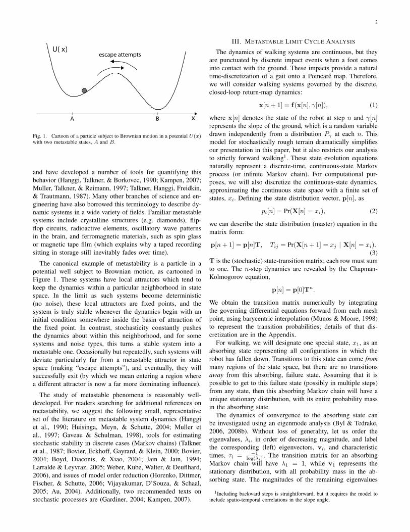

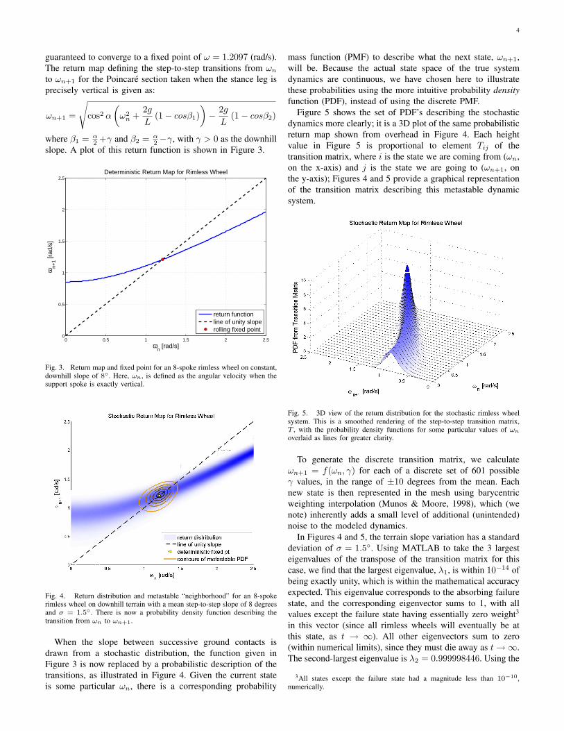
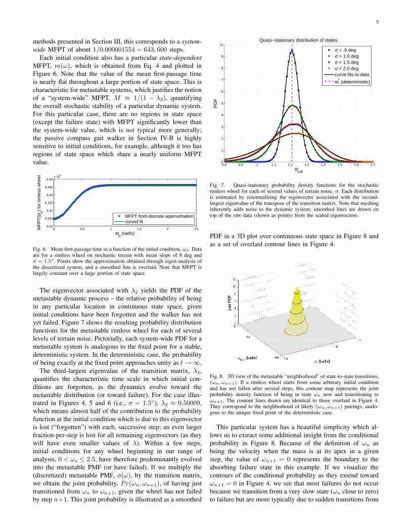

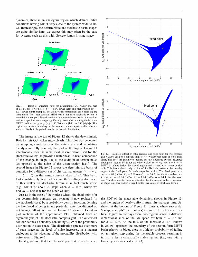

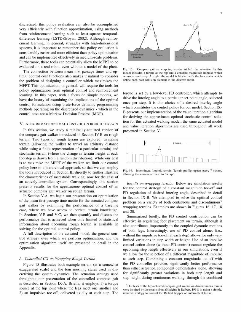
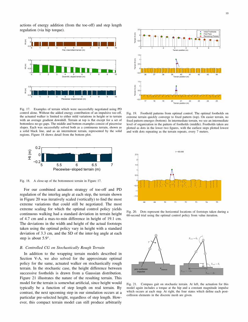
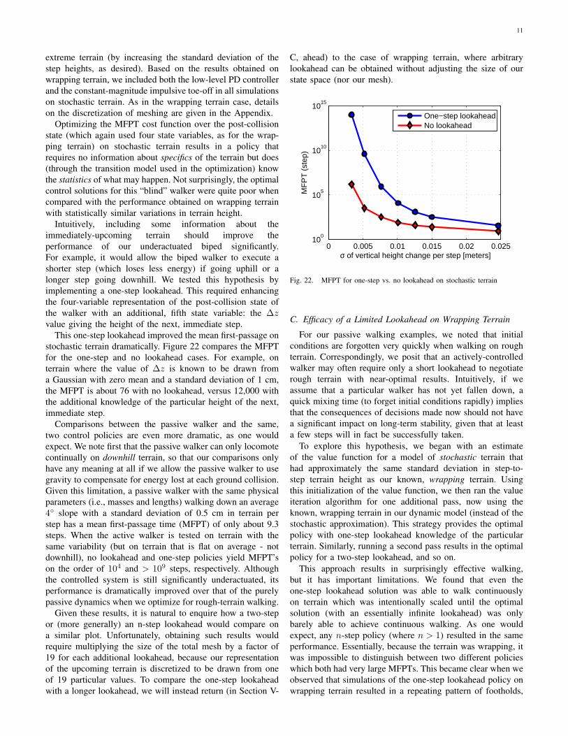
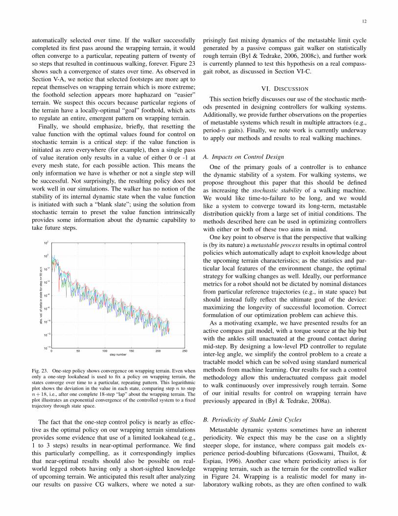

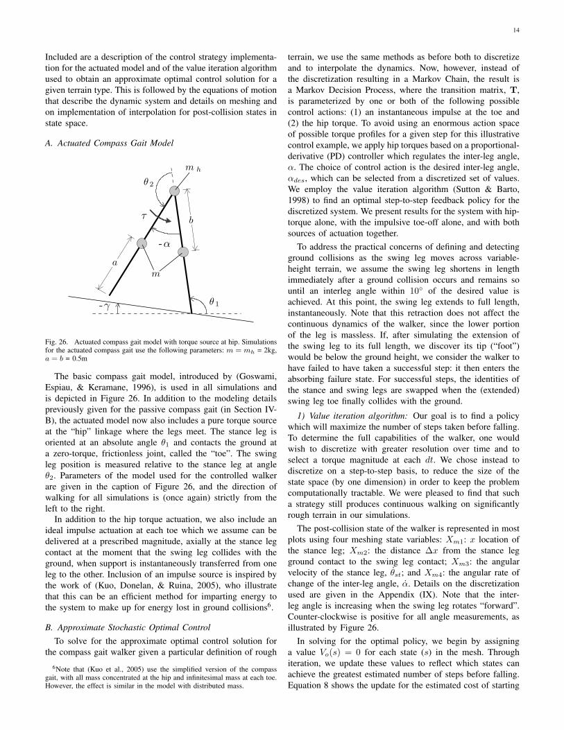


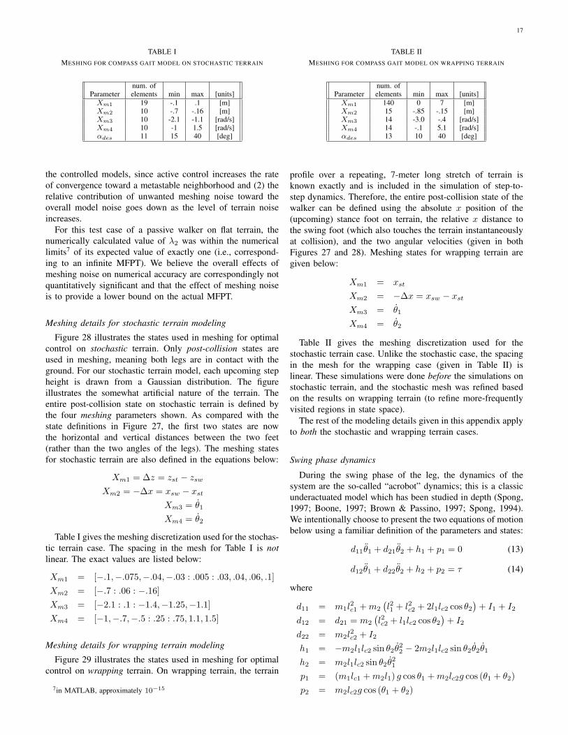
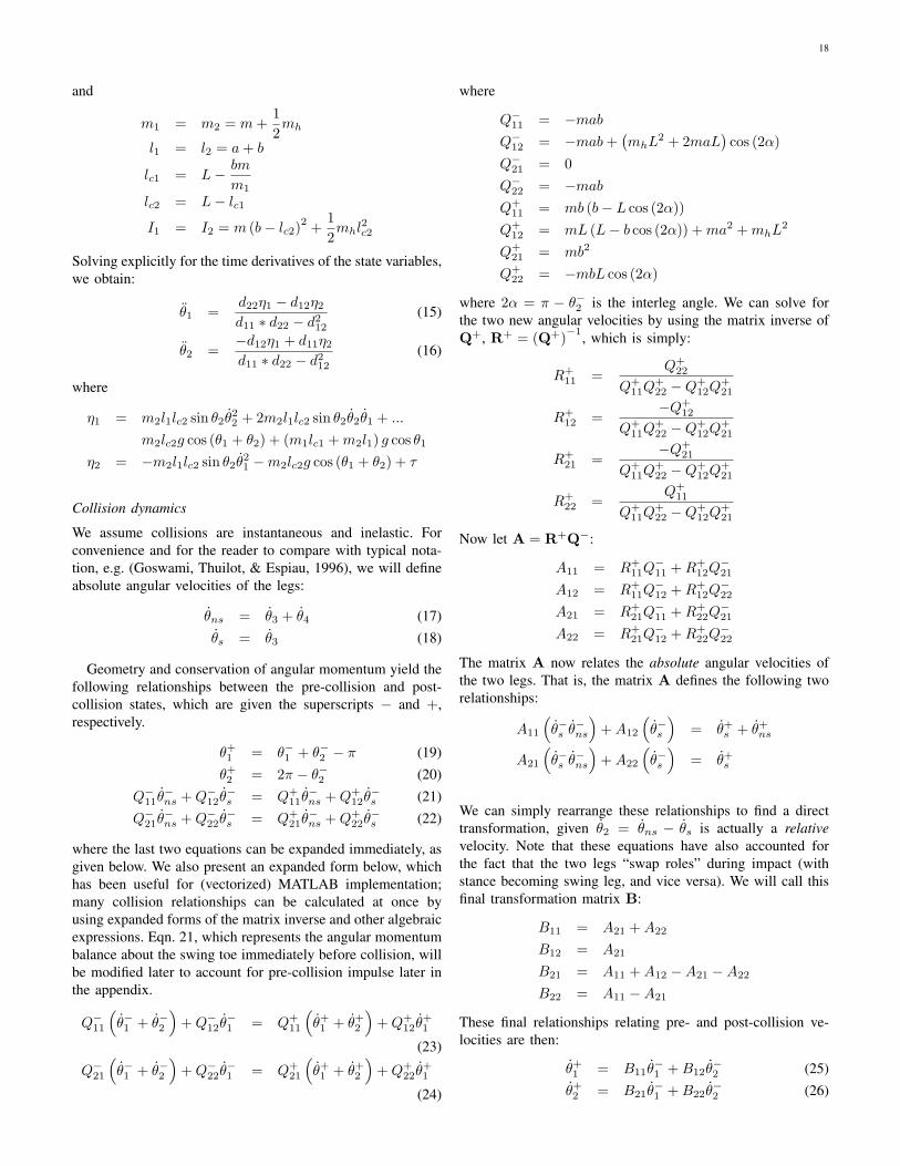

![Anextensivereviewofvibrationmodellingofrollingelementbeari ...data.mecheng.adelaide.edu.au/avc/publications/public_papers/2015/... · localisedandextendeddefects ... [170], ANSI (American](https://static.documents.pub/doc/80x56/5add2ae77f8b9aa5088c7ca7/anextensivereviewofvibrationmodellingofrollingelementbeari-data-170-ansi.jpg)


