224
METEOROLOGICAL CAUSES. OF ANOMALOUS MICROWAVE PROPAGATION T. Jones A thesis submitted in fulfilment of the requirements for the degree of Ph.D to the University of Edinburgh 1993 l b ovc%

METEOROLOGICAL CAUSES.
OF ANOMALOUS MICROWAVE
PROPAGATION
T. Jones
A thesis submitted in fulfilment of the requirements
for the degree of Ph.D
to the
University of Edinburgh
1993
lb ovc%

The echoes were abnormally strong today. Instead of slicing straight on
out into space as the curve of the earth fell away beneath it, the radar
beam was being bent downwards by some peculiarity of the atmosphere. It
was wa.vehopping all the way across the North Sea., bouncing off the Dutch
coast, and a. little more than a, thousandth of a second after it had started
its journey - returning along the same curving path with the secrets it had
gathered.
Glide Path
Arthur C. Clarke
1963

Declaration
This thesis has been composed by myself and it has not been submitted in any previous
application for a degree. The work reported within was executed by myself, unless
otherwise stated.
July 1993

Abstract
This thesis is concerned with the influence of the weather on radio signals on surface-
to-surface paths, looking particularly at the effects of fronts. The radio-meteorology
of anticyclones is well understood [COST 1991], but that of fronts is less so, despite
the knowledge that fronts can sometimes cause very severe radio interference through
anomalous signal propagation (anaprop).
A statistical analysis is made of two years signal data from seven paths in the UK and
to the Netherlands. By classifying weather conditions into 24 different types, the effects
of different types of weather as causes of anaprop have been determined. The results
confirm the belief [Bye 1988a] that the majority of anaprop occurs under anticyclonic
conditions, and that fronts are a relatively insignificant cause of anaprop. The results
for the different weather and path types are presented in a set of 'interference data
sheets', allowing rapid comparison of the effects of different weather conditions on
signals for land and sea paths. This analysis is one of only two that examine the effects
of different weather conditions on signals, and considers a far greater amount of both
signal and weather data than the other study [Spillard 1991].
To examine how fronts can cause anaprop, existing meteorological conceptual models
[e.g. Browning 19851 are adapted to show where super-refractive layers occur. The
models examine ana- and kata-fronts (both warm and cold), as well as warm and cold
occlusions. For each type of front, qualitative predictions of the liklihood of anaprop
are given.
The conceptual models are verified in two ways. Using dropsoude data from the
FRONTS'87 project, three fronts are examined at resolutions far higher than can be
obtained from routine observations. Super-refractive layers are found where the con-
ceptual models predict them, and it is possible to make estimates of the location and
strength of these layers. Using routine meteorological observations and signal data,
it is found that, when fronts cause anaprop, the signals occur where predicted by the
models. It is found, however, that only some 50% of fronts actually cause anaprop, but
it is not yet clear why this is so.
111

Acknowledgements
I acknowledge the copyright of all the authors and organisations whose diagrams are
reproduced in this work. All these are identified in the text.
I would like to thank everyone who has helped me during the course of this work,
especially:
Dr. Keith Weston (Edinburgh University) and Dr. Mick Mehier (BTL) for their super-
vision of this thesis.
Gail Bye and Bob Howell (BTL) for their help and advice throughout the project.
Drs. Sid Clough and John McKay (Meteorological Office) for allowing me access to the
FRONTS'ST data used in Chapter 5.
Special mentions to all my friends who have provided so much support and encourage-
ment over the last few years.
This work was funded and carried out under British Telecom
research contract A039339/1'.
The author is now at:
Department of Mathematics
Peterhead Academy
Prince Street, Peterhead
ABERDEENSHIRE, AB42 6QQ
iv

Contents
1 Introduction 1
1.1 The need for this research ..........................1
1.2 Outline of the thesis .............................4
1.2.1 Original material in this thesis ...................5
1.3 Summary of findings .............................5
2 Literature Survey 7
2.1 Radio propagation .............................. 7
2.1.1 Signal attenuation .......................... 8
2.1.2 Signal paths .............................. 9
2.2 Atmospheric refractivity ........................... 12
2.2.1 The radio refractive index ...................... 12
2.2.2 Presentation of refractivity da.ta................... 13
2.2.3 Refractivity regimes ......................... 16
2.2.4 Ducting ................................ 17
2.2.5 Duct meteorology .......................... 20
2.3 Radio-meteorology .............................. 22
2.3.1 Subsidence .............................. 22
2.3.2 Offshore Advection .......................... 23
2.3.3 Sea. breeze a.dvection ......................... 24
2.3.4 Nocturnal radiation cooling ..................... 25
2.3.5 Evaporation ducts .......................... 26
2.4 The radio-meteorology of anticyclones ................... 26
2.4.1 Anticyclones and a.naprop ...................... 27
2.4.2 The meteorology of anticyclones .................. 28
2.4.3 The BTL anticyclone model ..................... 29
2.5 The radio-meteorology of fronts ....................... 32
2.5.1 Fronts and a.na.prop ......................... 32
2.5.2 'Sporadic' subsidence ......................... 36
3 Statistical analysis of weather and anaprop 39
V
3.1 Previous work 40
3.1.1 Statistical analyses .......................... 40
3.1.2 Prediction methods .......................... 41
3.I.:3 Presentation of signal data ..................... 41
3.2 Data analysis ................................. 42
3.2.11 Selection of data ............................ 42
3.2.2 Weather classification ........................ 43
3.2.3 Verification of the weather classification scheme .......... 46
3.2.4 Data analysis ............................. 47
3.3 Results of analysis .............................. 47
3.3.1 Expected results ........................... 48
3.3.2 Occurrence of (liflerdnt. weather conditions ............. 49
3.3.3 Significance of signals ........................ .50
3.3.4 Interference Da.ta Sheets ....................... 52
3.3.5 Results for Dutch signal paths ................... 52
3.3.6 Results for UK signal paths ..................... 56
3.4 Discussion ................................... 59
3.4.1 Occurrence of different weather conditions ............. 59
3.4.2 Significance of signals ........................ 59
3.4.3 Interference data sheets ....................... 60
3.4.4 Dutch signal paths .......................... 60
3.4.5 UK signal paths ........................... 61
3.4.6 Conclusions .............................. 62
4 Conceptual models of fronts and anaprop 64
4.1 Meteorological Models of Fronts ....................... 65
4.1.1 'Conveyor Belt' Models ....................... 66
4.2 Adaptations of models for Radio-Meteorological use ........... 70
4.2.1 Objectives ............................... 71
4.2.2 Anapiop associated with Fronts ................... 71
4.2.3 Effects of surface temperature .................... 73
4.2.4 A word of warning! .......................... 74
4.3 Depressions with Ana-fronts ......................... 74
4.3.1 Structure ............................... 74
4.3.2 Expectations of anaprop ....................... 76
4.3.3 Discussion ............................... 77
4.4 Kata-type depressions without an Upper Cold Front ........... 77
4.4.1 Structure ............................... 77
4.1.2 Expectations of anaprop ....................... 77
4.4.3 Discussion ............................... 79
VI
4.5 Kata-type depressions with an Upper Cold Front 79
4.5.1 Structure ................................ 80
4.5.2 Expectations of aliaprop ....................... 81
4.5.3 Discussion ............................... 82
4.6 Occluded depressions ............................. 82
4.6.1 Warm occlusions ............................. 82
4.6.2 Cold occlusions ............................ 83
4.6.3 Discussion ............................... 85
4.7 Warm sector subsidence ........................... 85
5 Refractivity analysis I—FRONTS'87 86
5.1 The FRONTS'ST Project .......................... 86
5.1.1 The field experiment ......................... 87
5.1.2 The Intensive Observational Periods ................ 88
5.1.3 Instruments .............................. 89
5.2 Radio-Meteorological Studies ........................ 90
5.2.1 Data Processing ........................... 90
5.3 lOP 7 Case Study .............................. 93
5.3.1 Run 1 ................................. 94
5.3.2 Run 2 ................................. 94
5.3.3 Run 3 ................................. 97
5.3.4 Run 4 ................................. 97
5.3.5 Summary ............................... 97
5.4 lOP $ Case Study .............................. 101
5.4.1 Run I ................................. 101
5.4.2 Run 2 ................................. 103
5.4.3 Run 3 ................................. 103
5.4.4 Run 4 ................................. 106
5.4.5 Summary ............................... 106
5.5 lOP 4 Case Study .............................. 109
5.5.1 Run 2 .................................. 109
5.5.2 Run 3 ................................. 111
5.5.3 Run 4 ................................. 111
5.5.4 Summary ............................... 111
5.6 Discussion ................................... 115
6 Refractivity analysis II—Gt Baddow 116
6.1 Sources of Data ................................117
6.2 Data analysis .................................118
6.2.1 Signal data analysis .........................118
VII

6.2.2 Weather data. analysis 119
6.3 Correlation of surface data with signals .................. 120
6.3.1 Cold fronts parallel to the path ................... 121
6.3.2 Cold fronts perpendicular to the path ............... 122
6.3.3 Warm fronts ............................. 126
6.4 Correlation of refractivity sections with signals .............. 127
6.4.1 Selection of case studies ....................... 127
6.4.2 Analysis of a refractivity cross section ............... 128
6.4.3 Analysis of a refractivity time section ............... 130
6.5 Discussion ................................... 131
6.5.1 Surface analysis ............................ 131
6.5.2 Refractivity analysis ......................... 133
7 Conclusions 135
7.1 Summary of findings ..............................35
7.2 Further work .................................139
7.3 Evaluation ...................................141
A Interference data sheets 143
B Publications and reports 193
B.1 Reports ....................................193
B.2 Published Papers ...............................195
C Bibliography
'RXITI,
vilt
List of Figures
1.1 Long-term causes of anaprop 2
1.2 Short-term causes of anaprop ........................ 3
2.1 Signal attenuation from atmospheric absorption .............. 9
2.2 Attenuation due to rain ........................... 10
2.3 Signal paths set up for the COST 210 project ............... 11
2.4 Comparison of P EU and lUtE structures .................. 15
2.5 Radio and optical horizons .......................... 16
2.6 Refractivity regimes ............................. 17
2.7 Signal propagation in ducts ......................... 18
2.8 Refractivity profiles through ducts ..................... 20
2.9 Temperature and moisture profiles through ducts ............. 21
2.10 The BTL anticyclone model ......................... 29
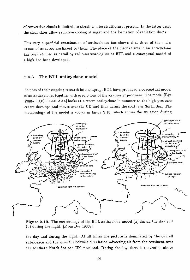
2.11 BTL model predictions for a sea path .................... 30
2.12 BTL model predictions for a. land path ................... 31
2.13 BTL model predictions for a. coastal path ................. 31
2.14 Refractivity structure near a cold front ................... 34
2.15 Refractivity structure near a warm front ................... 35
2.16 Refractivity structure of a 'sporadic subsidence' event .......... 37
2.17 Signal behaviour during a. 'sporadic subsidence' event .......... 37
2.18 Refractivity structure of a 'sporadic subsidence' event on a land path 38
3.1 Relationship between signal paths and weather conditions ........ 44
3.2 Significance ratios for Dutch signal paths ................. 51
3.3 Significance ratios for UN signal paths ................... 51
3.4 Cumulative distributions of signals on Dutch paths ............ 53
3.5 Annual distribution of signals on Dutch paths ............... 54
3.6 Diurnal distribution of signals on Dutch paths ............... 55
3.7 Cumulative distributions of signals on UK paths ............. 56
3.8 Annual distribution of signals on UK paths ................ 57
3.9 Diurnal distribution of signals on UK paths ................ 58
Ix
4.1 Ana.- and ka.ta- fronts 65
4.2 Warm and cold occlusions ........................... 66
4.3 Conveyor belts in a mid-latitude depression ................ 67
4.4 Cold front with rearwards sloping ascent .................. 68
4.5 Cold front with forwards sloping ascent .................. 69
4.6 Types of super-refractive layers associated with depressions . . . . . . . . 72
4.7 Effects of surface temperature on SRLs ................... 73
4.8 Plan of a typical depression with a.na-fronts ................ 75
4.9 Cross section through a depression with ana-fronts ............ 75
4.10 Anaprop in a depression with a.na-fronts .................. 76
4.11 Plan of a typical depression with kata-fronts ................ 78
4.12 Cross-section through a. depression with ka.ta-fronts ............ 78
4.13 Anaprop in a typical depression with kata-fronts ............. 79
4.14 Plan of a, typical depression with kata.- fronts and an tipper cold front 80
4.15 Cross section through a. depression with kata-fronts and an upper cold
front...................................... 81
4.16 Anaprop in a. depression with kata-fronts and an upper cold front . . . 81
4.17 Section through a. typical warm occlusion showing the location of SRLs 83
4.18 Expectations of a.na.prop in a warm occlusion................ 83
4.19 Section through a typical cold occlusion showing the location of SRLs. 84
4.20 Expected probability of anaprop in a cold occlusion ............ 84
5.1 The FRONTS'87 experimental area . . . . . . . . . . . . . . . . . . . . . 88
5.2 Met Office temperature analysis ....................... 92
5.3 Author's temperature analysis ........................ 93
5.4 lOP 7 run 1 O section ............................ 95
5.5 lOP 7 run 1 PRI section ........................... 95
5.6 lOP 7 run 2 Ge section ............................ 96
5.7 lOP 7 run 2 FRI section ........................... 96
5.8 lOP 7 run 3 0 section ............................ 98
5.9 lOP 7 run 3 PR.1 section ........................... 98
5.10 TOP 7 run 4 G section ............................ 99
5.11 lOP 7 run 4 PR1 section ........................... 99
5.12 lOP 7 dropsondes and location of SRLs .................. 100
5.13 SRLs observed during lOP 7 ........................ 100
5.14 lOP S Run 1 Ge section ........................... 102
5.15 lOP S Run 1 PRI structure ......................... 102
5.16 lOP 8 run 2 O section ............................ 104
5.17 lOP S Run 2 PRI structure ......................... 104
5.18 lOP S Run 3 0, section ........................... 105
x
5.19 lOP S Run 3 PRA structure 105
5.20 lOP S run 4 G section ............................. 107
5.21 lOP 8 Run 4 FRI structure ......................... 107
5.22 lop S dropsonde runs, frontal positions and SilLs ............ 108
5.23 Summary of SilLs observed for lop 8 ................... 108
5.24 lop 4 run 2 O section ............................ 110
5.25 lop 4 Run 2 PRI structure ......................... 110
5.26 lOP 4 run 3 O section ............................ 112
5.27 lOP 4 Run 3 Pill structure ......................... 112
5.28 lOP 4 lUll 4 Ge section ............................ 113
5.29 lOP 4 Run 4 PR.I structure ......................... 113
5.30 lop 4 clropsonde runs, frontal positions and SilLs ............ 114
5.31 Summary of SRLs from lOP 4 ....................... 114
6.1 The Ct Baddow-Martlesha.rn signal path ................... 18
6.2 Cold front parallel to path - no a.iiaprOp ................. 122
6.3 Cold (rout parallel to path - single period of a.na.prop .......... 123
6.4 Cold front parallel to path - two periods of anaprop ........... 123
6.5 Cold front perpendicular to path - no anaprop .............. 124
6.6 Cold front perpendicular to path - one period of anaprop ........ 125
6.7 Cold front perpendicular to path - two periods of anaprop ....... 126
6.8 Warm front parallel to path ......................... 127
6.9 Cross section analysis-signal behaviour .................. 129
6.10 Cross section analysis-refractivity structure ............... 129
6.11 Time section analysis-signal behaviour .................. 132
6.12 Time section analysis-refractivity structure ................ 132
7.1 Significance ratios for Dutch signal paths ................. 136
7.2 Significance ratios for UK signal paths ................... 136
7.3 Real and expected SR.Ls at an ana-cold front ................. .38
7.4 Real and expected SilLs at a kata-cold front ................ 13$
7.5 Real and expected SRLs in a warm occlusion ................. .39
xl
List of Tables
3.1 Signal paths used for statistical analysis in this work 43
3.2 Occurrence of different weather types on Dutch and UK paths .....49
5.1 The FRONTS'ST Intensive Observational Periods [Macun 1988] 89
5.2 lOP 7 Dropsonde runs [Machin 1988] ....................94
5.3 lOP 7 Dropsonde runs [Macun 1988] ....................101
5.4 lOP 4 Dropsoiicle runs [Machin 19881 ....................109
6.1 Fronts affecting the Ct Ba.cldow path. July-September 1989 .......119
XII

Chapter 1
Introduction
The object of this thesis is to investigate the part different weather conditions, in partic-
ular fronts, play in causing interference between different parts of a telecommunications
network. This chapter begins with the motivation behind this research, followed by an
outline of the remainder of the thesis and finally by a summary of the main findings.
1.1 The need for this research
This work has been undertaken at the request of British Telecom Laboratories (BTL),
and forms part of their continuing investigation of the effects of the Earth's atmosphere
on radio propagation. This sort of work is important since the radio and microwave
regions of the electromagnetic spectrum are limited in extent and are in demand for a
wide variety of uses, from broadcasting to radio astronomy. As a result there is con-
siderable pressure to minimise 'wastage' of the spectrum. British Telecom, in common
with most telecommunications agencies in the developed world, uses microwaves for
point to point communications, beaming signals along line of sight paths typically 50
to 100 km in length. To avoid interference, nearby paths must use different frequen-
cies and the object of BTL's research is to minimise the coordination distance within
which a frequency cannot be reused without unacceptable amounts of interference be-
tween the paths'. The coordination distance depends on both geographical factors
- the geometry of the paths and the underlying terrain - and on the meteorology,
through a number of interference propagation mechanisms in the atmosphere. These
'"Unacceptable" amounts are difficult to quantify, but typically are when interference occurs for more than 0.1% of the year [Hall 1979 p1791.
1
mechanisms can be divided into long-term (hence of importance when planning signal
networks) and short-term (unpredictable and often producing very severe interference)
mechanisms [COST 1991 p2.11.
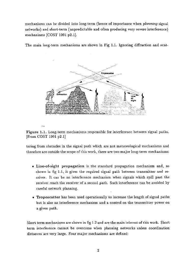
The main long-term mechanisms are shown in Fig 1.1. Ignoring diffraction and scat-
. : Troer
Une rv of
sight
- --_
Figure 1.1. Long-term mechanisms responsible for interference between signal paths. [From COST 1991 p2.1]
tering from obstacles in the signal path which are not meteorological mechanisms and
therefore are outside the scope of this work, there are two major long-term mechanisms:
• Line-of-sight propagation is the standard propagation mechanism and, as
shown in fig 1.1, it gives the required signal path between transmitter and re-
ceiver. It can be an interference mechanism when signals which spill past the
receiver reach the receiver of a second path. Such interference can be avoided by
careful network planning.
• Troposcatter has been used operationally to increase the length of signal paths
but is also an interference mechanism and a control on the transmitter power on
a given path.
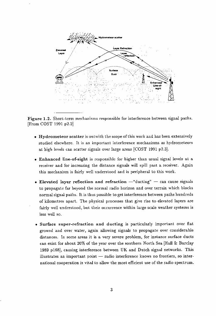
Short term mechanisms are shown in fig 1.2 and are the main interest of this work. Short
term interference cannot be overcome when planning networks unless coordination
distances are very large. Four major mechanisms are defined:
2
Hydrometeor scatter
Elevated Layer Refraction
Layer Layer rell
Suace
Duct
Line-of- sight
Figure 1.2. Short-term mechanisms responsible for interference between signal paths. [From COST 1991 p2.2]
• Hydrometeor scatter is outwith the scope of this work and has been extensively
studied elsewhere. It is an important interference mechanisms as hydrometeors
at high levels can scatter signals over large areas [COST 1991 p2.3].
• Enhanced line-of-sight is responsible for higher than usual signal levels at a
receiver and for increasing the distance signals will spill past a receiver. Again
this mechanism is fairly well understood and is peripheral to this work.
• Elevated layer reflection and refraction —"ducting" - can cause signals
to propagate far beyond the normal radio horizon and over terrain which blocks
normal signal paths. It is thus possible to get interference between paths hundreds
of kilometres apart. The physical processes that give rise to elevated layers are
fairly well understood, but their occurrence within large scale weather systems is
less well so.
• Surface super-refraction and ducting is particularly important over flat
ground and over water, again allowing signals to propagate over considerable
distances. In some areas it is a very severe problem, for instance surface ducts
can exist for about 20% of the year over the southern North Sea [Hall & Barclay
1989 p168], causing interference between UK and Dutch signal networks. This
illustrates an important point - radio interference knows no frontiers, so inter-
national cooperation is vital to allow the most efficient use of the radio spectrum.
3

The final two mechanisms are related, involving reflection and/or refraction from super-
refractive layers in the atmosphere. It is these mechanisms which are the main interest
of this work. Also, it should be remembered that these mechanisms operate together
and so interactions between different mechanisms can be as important as the individual
processes.
1.2 Outline of the thesis
This thesis looks at much of radio-meteorology, starting with an overview of the subject
and moving to a detailed study of the radio-meteorology of fronts. There are five main
chapters:
• Chapter 2 reviews the current state of knowledge of radio meteorology. It looks
at the essential details of radio propagation in the Earth's atmosphere and at
how certain weather conditions can cause anomalous propagation (anaprop).
The mechanisms responsible for anaprop are examined as is existing research
on anaprop due to anticyclones and fronts.
• Chapter 3 presents the results of an analysis of signal data for a number of paths
in North West Europe and correlates signal behaviour over a two-year period
with the prevailing weather conditions. After a discussion of the methods used to
analyse the signal and weather datasets, the results of the analysis are presented
and discussed. This analysis is one of the first to look at signal statistics under
different weather conditions rather than for a particular period, regardless of the
changing weather.
• Chapter 4 looks at conceptual models of fronts. Existing meteorological models
of depressions are examined and then adapted to radio-meteorology. Conceptual
models of the refractivity structure and the expected anaprop around all types of
fronts are presented here. These models are similar in idea to the BTL conceptual
model of an anticyclone, providing a framework for the case studies of frontal
anaprop in the final chapters of this work and also providing a basis for operational
predictions of anomalous propagation.
• Chapter 5 uses the conceptual models to analyse the detailed structure of ana-
and kata- cold fronts and an occlusion. Data have been obtained from the Mete-
orological Office's FRONTS'87 project and analysed to provide the first detailed
studies of the refractivity structure around these fronts.
4

• Chapter 6 contains a number of case studies of signal behaviour as fronts interact
with a short signal path in South East England. This path was selected since there
is very high resolution signal data for a period when there were a number of frontal
interference events and there were both upper air and surface meteorological data
available. The analysis looks both at the signal data and the refractivity structure
over the path. Again the conceptual models are used to interpret the findings.
1.2.1 Original material in this thesis
Being an interdisciplinary thesis, this work contains much material that has already
been published. This is necessary since the work may be used both by meteorologists
and by radio engineers and it is necessary to give each some background of the others
subject. This material is contained in chapter 2 as well as in the early part of chapter 4
Summarising the new material for each chapter:
• Chapter 3 presents the first examination of the effects of different weather con-
ditions on UK and Dutch signal paths. The only other work along these lines
[Spillard 1991] is a study of a much more limited number of weather types and
signal paths than this work.
• Chapter 4 takes existing meteorological conceptual models of fronts and adapts
them to radio-meteorology. This adaptation, together with the estimated proba-
bilities of anaprop associated with different types of fronts is entirely new.
• Chapter 5 contains entirely new material. No previous analysis of the detailed
refractivity structure around weather fronts has ever been made.
In chapter 6 the methods used to analyse the weather and signal data are not
new, but the application of them to fronts is.
• The Interference Data Sheets [Appendix A] are an entirely new idea. They repre-
sent the first attempt to give path planners a way of seeing the effects of different
weather conditions on the long term behaviour of anaprop.
1.3 Summary of findings
This section reviews the main results of each chapter of this thesis.
5

Chapter 3 looks at the statistics of anaprop in north west Europe under a wide range
of weather conditions. The results confirm the generally held belief that the majority
of anaprop occurs under anticyclonic conditions, but then goes further and looks at the
effects of the location of the high pressure centre and at differences between seasons.
Frontal conditions are found generally to give below average amounts of anaprop, but
there are some exceptions. Again seasonal differences are observed, but on the whole
they are less important than for anticyclonic conditions. Interactions of fronts with
anticyclones are important causes of anaprop, but they are not common enough to be
significant statistically.
Chapter 4 adapts meteorological models of fronts to radio- meteorology. The important
features are low level super-refractive layers ahead of warm fronts and behind cold
fronts. In the warm sector the refractivity structure depends on the type (ana-type or
kata-type) of the front. An occlusion has characteristics of warm and cold fronts. These
models are conceptual and give qualitative predictions of the likelihood of anaprop near
the front. The models can be used to account for all observations of frontal anaprop
in the published literature.
Chapter 5 begins the process of verifying the conceptual models, using high resolution
data from the FRONTS'87 project. Although not all types of fronts can be studied,
those that can be (ana- and kata-cold fronts, and an occlusion) show the features
expected from the conceptual models. This allows some values to be given to the
extent, position and strength of the super-refractive layers. Due to the variability of
fronts, the values obtained may not be typical, but they represent a much more detailed
study than has been made in the past.
Chapter 6 continues the verification of the conceptual models, linking the meteorology
to anaprop. Much of the observed signal behaviour can be explained by the models and
cross- and time-sections show how the refractivity structure is correlated to the signals.
The range of behaviour of the signals stresses the variability of fronts and brings home
the point that no front can be considered 'typical'.
An implicit, but generally unstated, goal of this work is to increase the links between
the very different disciplines of meteorology and radio-science. Each has much to offer
the other, and both should be willing to learn. Whether this goal has been achieved,
only time will tell.
6

Chapter 2
Literature Survey
A considerable amount of research has been done on the links between radio science and
meteorology since the development of radio early this century. This chapter examines
the current state of knowledge of the field, looking at several different areas. Much of
the existing research is, while interesting and important elsewhere, of little relevance
to the remainder of this thesis, which concentrates on the meteorological aspects of
anomalous propagation. Such material will be mentioned only in passing, with key
references provided for the reader who wishes to investigate further. Material important
later in the work will be explained in detail.
The literature survey begins with the basics of radio propagation and then looks at at-
mospheric refractivity, the major effect in radio-meteorology. This is followed by details
of the meteorological mechanisms which give rise to anaprop and then by summaries
of the current knowledge of the radio-meteorology of anticyclones and fronts.
2.1 Radio propagation
Radio waves (including the microwaves that are of particular interest in this work)
form part of the electromagnetic spectrum, with wavelengths between millimetres and
kilometres. Of most interest to this work is the short wavelength end of this range.
Radio signals are vital to all forms of telecommunications, ranging from radio and TV
broadcasts to point-to-point links on the Earth's surface or between the Earth and a
satellite.
7
dio signals propagate according to an inverse square law. _t6', 1$c IeJ • by factors such as the type of transmitting and receiving antennae and the medium
through which the signals travel. Further effects can come from terrain, which can block
or scatter signals. The physics of radio propagation, antenna design and terrain effects
are all outwith the scope of this research but can be found in many texts [e.g. Booker
& Walkinshaw 1947, Bean & Dutton 1966, Hall 1979, Boithias 1987, Hall & Barclay
1989].
For this research, signals transmitted in a narrow beam are the only type studied. This
allows us to consider the behaviour of signals as a problem in ray optics, rather than
having to use mode theory, and simplifies the physics side of the problem considerably.
2.1.1 Signal attenuation
A signal propagating through the atmosphere will suffer attenuation from two causes.
These are absorption by atmospheric gases and water droplets and scattering by aerosols 1
and turbulence. Under normal circumstances this attenuation is a problem, but it is
used to advantage in over-the-horizon troposcatter propagation [Spillard 19911.
At microwave frequencies atmospheric absorption is due to oxygen molecules and water
vapour. Attenuation depends on frequency as well as atmospheric pressure, tempera-
ture and humidity and can vary from almost nothing to as much as 40 dB/km. The
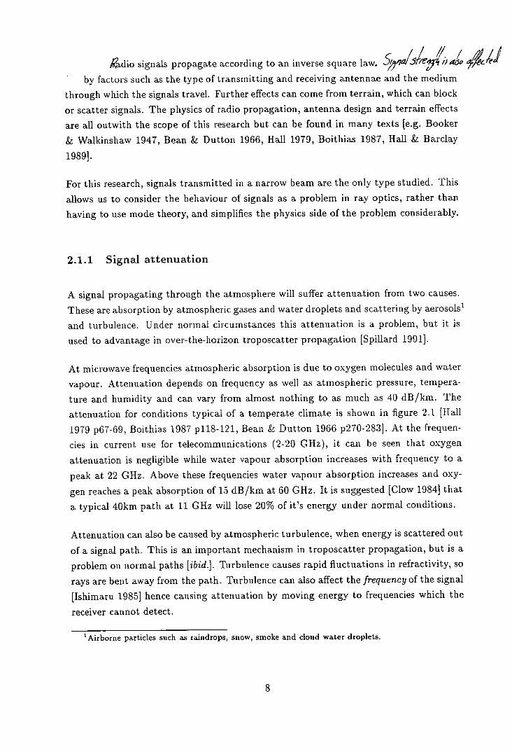
attenuation for conditions typical of a temperate climate is shown in figure 2.1 [Hall
1979 p67-69, Boithias 1987 p118-121, Bean & Dutton 1966 p270-283]. At the frequen-
cies in current use for telecommunications (2-20 GHz), it can be seen that oxygen
attenuation is negligible while water vapour absorption increases with frequency to a
peak at 22 GHz. Above these frequencies water vapour absorption increases and oxy -
gen reaches a peak absorption of 15 dB/km at 60 GHz. It is suggested [Clow 1984] that
a typical 40km path at 11 GHz will lose 20% of it's energy under normal conditions.
Attenuation can also be caused by atmospheric turbulence, when energy is scattered out
of a signal path. This is an important mechanism in troposcatter propagation, but is a
problem on normal paths [ibid.]. Turbulence causes rapid fluctuations in refractivity, so
rays are bent away from the path. Turbulence can also affect the frequency of the signal
[Ishimaru 1985] hence causing attenuation by moving energy to frequencies which the
receiver cannot detect.
'Airborne particles such as raindrops, snow, smoke and cloud water droplets.
E
C 0
0
C
0
U,
Specific attenuation -y 0 and -j due to oxygen and water vapour
a 70 + for f> 10GHz '
b - for f> 10 G Hz scale A
c70 for f>1OGHz )
d70 for f< 10GHz scale
Pressure: 1 atm (1013mb)
Temperature: 20 ° C Wuervaoour density: 7.5gm/rn 3 (i.e. 'w = 7w7.5)
10
20 50 100 200 350 2 5 10 (B)
Frequency ,Gl4z
Figure 2.1. Signal attenuation due to atmospheric absorption [From Hall 1979 p68].
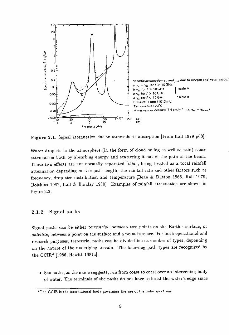
Water droplets in the atmosphere (in the form of cloud or fog as well as rain) cause
attenuation both by absorbing energy and scattering it out of the path of the beam.
These two effects are not normally separated [ibid.], being treated as a total rainfall
attenuation depending on the path length, the rainfall rate and other factors such as
frequency, drop size distribution and temperature [Bean & Dutton 1966, Hall 1979,
Boithias 1987, Hall & Barclay 1989]. Examples of rainfall attenuation are shown in
figure 2.2.
2.1.2 Signal paths
Signal paths can be either terrestrial, between two points on the Earth's surface, or
satellite, between a point on the surface and a point in space. For both operational and
research purposes, terrestrial paths can be divided into a number of types, depending
on the nature of the underlying terrain. The following path types are recognized by
the CCIR2 [1986, Hewitt 1987a].
• Sea paths, as the name suggests, run from coast to coast over an intervening body
of water. The terminals of the paths do not have to be at the water's edge since
'The CCIR is the international body governing the use of the radio spectrum.
9
100
150 mm/hr
50 mm/hr
101 I s.-- -
1 / / ,'_-------- 12.5 mm/hr
dB/kml / / If' ,'-_..-- 2.5 mm/hr
1
0.1
specific Attenuation in Rain Solid curves use Laws-Parsons DSD, dashed use Marshall-Palmer. 20 0C
0.01
1 10 100 1000
GHz
Figure 2.2. Attenuation of signals due to rain [From Hall & Barclay 1989 p1841
a path can be classified as sea type even if the terminals are a few kilometres
inland, provided there is no high terrain below the path.
• Land paths are those which are entirely above a land surface (rivers, streams
and minor water bodies are not enough to change the path type, but large water
bodies are [Hewitt 1987a]).
• Coastal paths are the most difficult to define. In general they run over land,
roughly parallel to the coastline. Further restrictions are that there should be
no high ground beneath the signal path. The CCIR have an official definition
of a coastal zone extending "50 km inland except where the terrain exceeds 100
metres altitude" [Bye 1988a], with all paths in this zone being coastal type. This
definition is not satisfactory, and various researchers have suggested alternative
definitions based on meteorological rather than geographical factors. These def-
initions suggest the coastal zone be defined by the furthest inland penetration
of sea air [Hewitt 1987a] or from climatological humidity statistics [Bye 1988a,
COST 1991]. Hewitt [1981] points out that coastal paths tend to have unique
propagation characteristics, so great care should be taken when discussing them
as a class.
• Mixed paths are a combination of the above types, for example most paths across
the Dover Straits will be mixed land-sea paths, land-type over the UK mainland,
with no coastal zone due to the height of the Downs, then sea type over the
10
Channel. It is suggested [Hewitt 1987b] that there should be a minimum of 40
km of a second terrain type before a path can be classified as 'mixed'.
• Operational paths are ones which carry telecommunications traffic. They are
generally short, typically 50 km long, with the terminals either in optical sight
of each other or slightly over the optical horizon'. For increased range, terminals
are often located on hills or on tall buildings, the London 'Telecom Tower' being
a prime example. To increase signal traffic, different polarizations may be used
simultaneously [Clow 19841. A large number of such terminals exist, covering the
UK (and much of the rest of the world) in an electronic web.
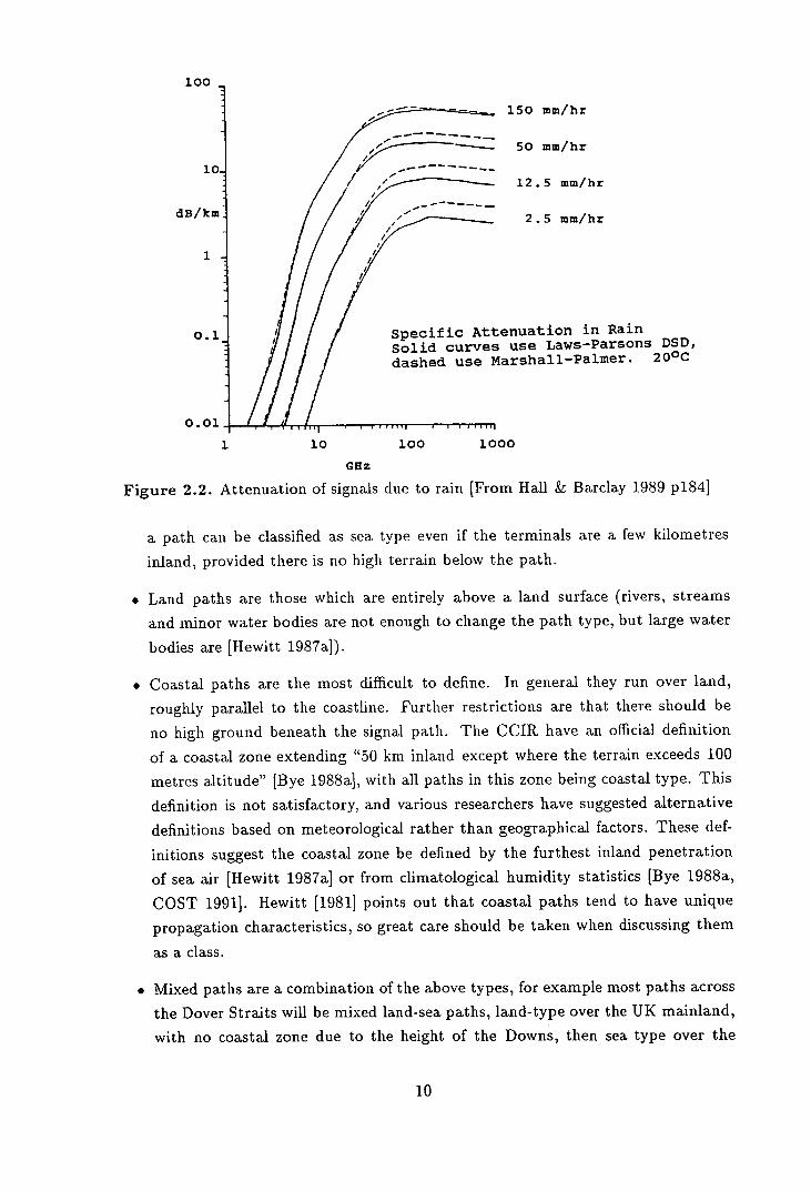
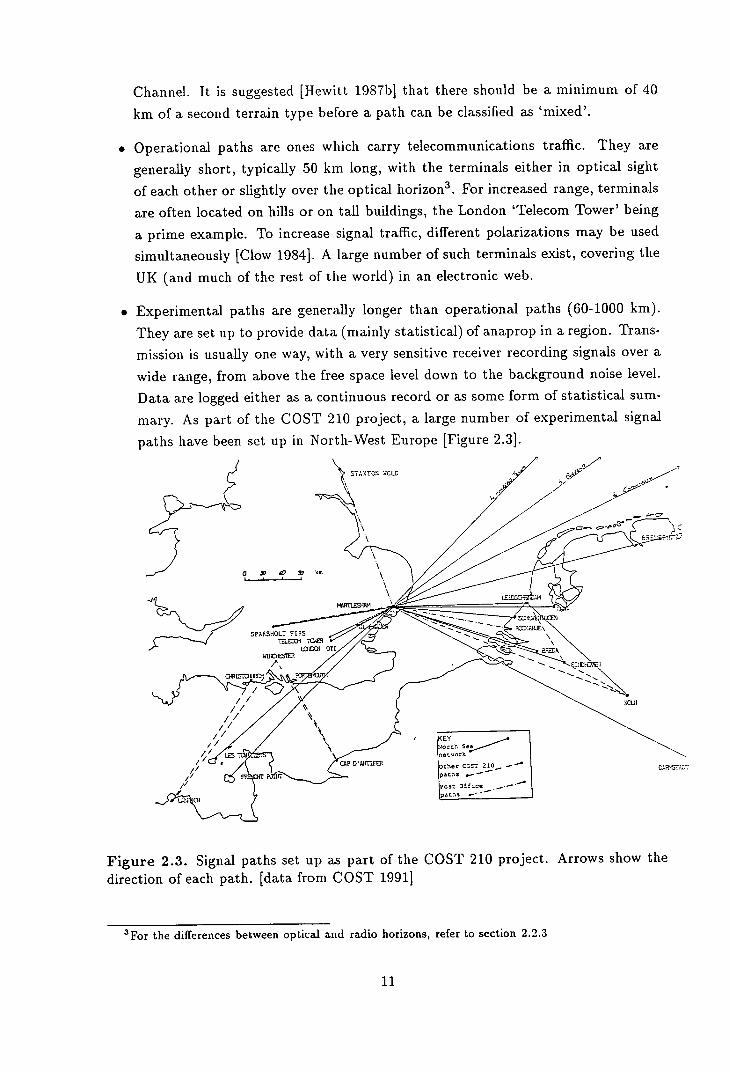
• Experimental paths are generally longer than operational paths (60-1000 km).
They are set up to provide data (mainly statistical) of anaprop in a region. Trans-
mission is usually one way, with a very sensitive receiver recording signals over a
wide range, from above the free space level down to the background noise level.
Data are logged either as a continuous record or as some form of statistical sum-
mary. As part of the COST 210 project, a large number of experimental signal
paths have been set up in North-West Europe [Figure 2.3].
STAXTON WCLD
C
\
SPASHOLT FLRS TELEM4 710.S
trfl:ol
cu'
D'MWIE CC5 2O_ —ther
ice
Figure 2.3. Signal paths set up as part of the COST 210 project. Arrows show the direction of each path. [data from COST 1991]
'For the differences between optical and radio horizons, refer to section 2.2.3
11
2.2 Atmospheric refractivity
Just as light rays are subject to reflection and refraction, so are radio waves, and the
atmospheric refractive index is the main control on anaprop.
2.2.1 The radio refractive index
Under 'typical' meteorological conditions, the atmosphere near the surface has a radio
refractive index, a, of about 1.00035, with a range of about ±0.0001. It is therefore
more convenient to consider the atmospheric refractivity, N, given by:
N = 106(n - 1)
(2.1)
T 'typical' refra tL
ivit is therefore about 359 N-units LCCIR 198 p1071. h2 C4' i " are it
The refractivity is a function of the temperature and the partial pressures of dry air,
carbon dioxide and water vapour, but it has been found that, under the range of
meteorological conditions found near the surface, the refractivity can be determined
to an accuracy of 0.02% from temperature (in Kelvins),
pressure (in mb) and vapour pressure (also in mb) by the equation:
P e (2.2)
where c = 77.6 and 3 = 373000 [Bye 1988a]. Equation 2.2 is sometimes given in the
form:
N = 77.6 ( P + 4810) (2.3)
Equation 2.3 has been accepted by the CCIR as the international standard method of
determining the refractivity from meteorological data [CCIR 1986 p107].
The accuracy of 0.02% quoted above assumes completely accurate meteorological mea-
surements. Such measurements are an unobtainable ideal, particularly in the upper air
observations that are of most interest to radio-meteorologists (see, for example, Hall
& Gardiner [1968], Ryder et.al. [1983], Nash & Schmidlin [1987] and Thompson [1989]
for discussions of the accuracy of upper air data
,±0 12' e.ts-,'o% For typical atmospheric conditions near the surface (P = 1000 mb, T = 288K and U
= 70%), the total error in RRI is given by equation 2.4 [Hall 1979 p20].
9N = 0.270P - 139T + 4.5& (2.4)
12
It can be seen that the vapour pressure is the source of most of the inaccuracy, which
is unfortunate since this is also the most difficult quantity to measure accurately.
The RRI can also be measured directly using refractometers. These are very accurate
(to about 0.01 N-unit) instruments [Bean & Dutton 1966 p30-7, Hall 1979 p19] and
have been used very successfully in the field [e.g. Levy et.al. 19911. Refractometers
are expensive instruments, so are not used for routine upper air observations, and no
refractometer data have been used in the course of this work.
2.2.2 Presentation of refractivity data
As altitude increases, atmospheric pressure falls as, on average, do temperature and
moisture content. The result is a systematic decrease in refractivity with height (the
refractivity lapse). In a well mixed atmosphere this decrease is exponential in form and
can be well represented by: N = N3 expz/z o ) (2.5)
where: N 3 is the surface RRI,
z (sometimes given as h) is the altitude,
zo is a scale height.
N 3 and zo vary with place and season, and radio-climatological maps exist showing
these variations [e.g. Bean & Dutton 1966 ch 4, DNOM 19841. The CCIR has defined
a reference atmosphere:
N = 315 exp(—z/7.36) (2.6)
where z is in km.
Other works [e.g. Hough 19 761 use the ICAN standard atmosphere with a constant
relative humidity of 80% as a reference atmosphere.
Several methods have been developed to present refractivity data. All have the common
aim of trying to emphasise small variations in refractivity and de-emphasise the large-
scale refractivity lapse. These methods have been well documented elsewhere [e.g. Bean
& Dutton 1966 p13-20] and have led to the following units used to define refractivity:
. The A-unit
. The B-unit
. The N0-unit
13
. The M-unit
. The K-unit
Only the latter two are of importance to this work.
The M-Unit
This method assumes that a horizontally launched ray will travel parallel to the Earth's
surface, giving a modified refractivity:
M=N +106 (z/a) (2.7)
where a is the Earth's radius (6371 km). This is often written as:
M = N + 157z
(2.8)
A refractivity profile in M-units clearly identifies the trapping level [Section 2.2.3] as
all layers where dM/dz < 0 [Turton et.al. 1988].
The K-unit
The K-unit, alone of all the other methods, which assume some sort of standard atmo-
sphere, uses actual meteorological data. It is common meteorological practice to con-
sider the potential temperature—the temperature a parcel of air would have if brought
adiabatically to a standard pressure level (usually 1000 mb). This method has been
applied to refractivity [Flavell 1962], allowing the preservation of the detailed structure
while removing the effects of the overall lapse. -
Potential temperature is given by:
9- T (1000) R1Cp
(2.9)
where R is the gas constant of air (287J kg- 'K - ') and C7, is the specific heat of air at
constant pressure (1.01 x 10³Jkg 1 Ii 1 )
Using the potential temperature, we can define the potential refractive index, or PRI,
as the refractivity if the temperature and moisture were reduced adiabatically to 1000
14
mb:
K = 77.6 ()
+ 3.73 x 10⁵()
(2.10)
where e0 = e(10001P).
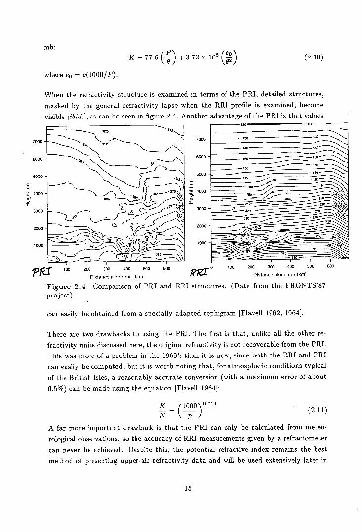
When the refractivity structure is examined in terms of the PRI, detailed structures,
masked by the general refractivity lapse when the RRI profile is examined, become
visible [ibid.], as can be seen in figure 2.4. Another advantage of the PIU is that values
7000
6000 - 6S
5000
E
4000 275
C)
275
3000
2000
1000 3
05
325
J30 130
—140 4o
160 —160
170
18O
—180
210
220 - 230'~
11 —240 250
260
- -33O —=
7000
6000
5000
E 4000
0) a, I
3000
2000
1000
0 100 200 300 400 UU 100 200 300 400 500 600
Distance alonq run (km) Distance alr,nn nm (km )
Figure 2.4. Comparison of PRI and RRI structures. (Data from the FRONTS'87 project)
600
can easily be obtained from a specially adapted tephigram [FIavell 1962, 19641.
There are two drawbacks to using the PRI. The first is that, unlike all the other re-
fractivity units discussed here, the original refractivity is not recoverable from the PRI.
This was more of a problem in the 1960's than it is now, since both the RRI and PRI
can easily be computed, but it is worth noting that, for atmospheric conditions typical
of the British Isles, a reasonably accurate conversion (with a maximum error of about
0.5%) can be made using the equation [Flavell 19641:
K = (1000)0 . 714 (2.11)
A far more important drawback is that the PRI can only be calculated from meteo-
rological observations, so the accuracy of RRI measurements given by a refractometer
can never be achieved. Despite this, the potential refractive index remains the best
method of presenting upper-air refractivity data and will be used extensively later in
15
this work.
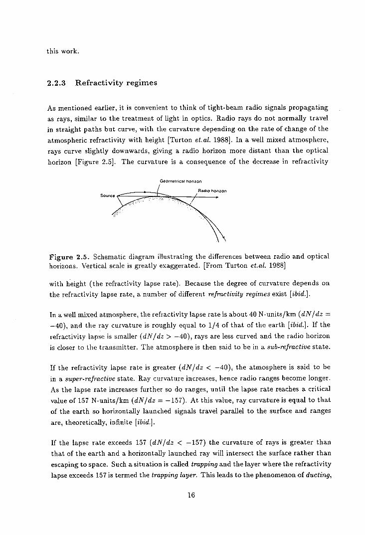
2.2.3 Refractivity regimes
As mentioned earlier, it is convenient to think of tight-beam radio signals propagating
as rays, similar to the treatment of light in optics. Radio rays do not normally travel
in straight paths but curve, with the curvature depending on the rate of change of the
atmospheric refractivity with height [Turton et.al. 1988]. In a well mixed atmosphere,
rays curve slightly downwards, giving a radio horizon more distant than the optical
horizon [Figure 2.5]. The curvature is a consequence of the decrease in refractivity
Geometrical horizon
Sour(
Figure 2.5. Schematic diagram illustrating the differences between radio and optical horizons. Vertical scale is greatly exaggerated. [From Turton et.al. 1988]
with height (the refractivity lapse rate). Because the degree of curvature depends on
the refractivity lapse rate, a number of different refractivity regimes exist [ibid.].
In a well mixed atmosphere, the refractivity lapse rate is about 40 N-units/km (dN/dz = —40), and the ray curvature is roughly equal to 1/4 of that of the earth [ibid.]. If the
refractivity lapse is smaller (dN/dz > — 40), rays are less curved and the radio horizon
is closer to the transmitter. The atmosphere is then said to be in a sub-refractive state.
If the refractivity lapse rate is greater (dN/dz < — 40), the atmosphere is said to be
in a super-refractive state. Ray curvature increases, hence radio ranges become longer.
As the lapse rate increases further so do ranges, until the lapse rate reaches a critical
value of 157 N-units/km (dN/dz = — 157). At this value, ray curvature is equal to that
of the earth so horizontally launched signals travel parallel to the surface and ranges
are, theoretically, infinite [ibid.].
If the lapse rate exceeds 157 (dN/dz < — 157) the curvature of rays is greater than
that of the earth and a horizontally launched ray will intersect the surface rather than
escaping to space. Such a situation is called trapping and the layer where the refractivity
lapse exceeds 157 is termed the trapping layer. This leads to the phenomenon of ducting,
16
one of the major causes of anaprop [ibid.].
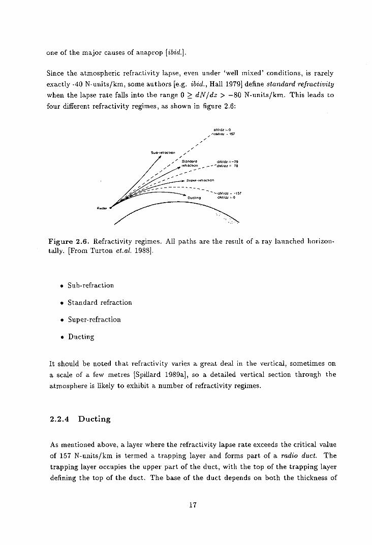
Since the atmospheric refractivity lapse, even under 'well mixed' conditions, is rarely
exactly -40 N-units/km, some authors [e.g. ibid., Hall 1979] define standard refractivity
when the lapse rate falls into the range 0 > dN/dz > —80 N-units/km. This leads to
four different refractivity regimes, as shown in figure 2.6:
dNIdz 0 'dM/di - 157
/
,
Sub-reiraclion
Standard dN/dz =-79
Radar
Figure 2.6. Refractivity regimes. All paths are the result of a ray launched horizon-tally. [From Turton et.al. 1988].
. Sub-refraction
. Standard refraction
• Super-refraction
• Ducting
It should be noted that refractivity varies a great deal in the vertical, sometimes on
a scale of a few metres [Spillard 1989a], so a detailed vertical section through the
atmosphere is likely to exhibit a number of refractivity regimes.
2.2.4 Ducting
As mentioned above, a layer where the refractivity lapse rate exceeds the critical value
of 157 N-units/km is termed a trapping layer and forms part of a radio duct. The
trapping layer occupies the upper part of the duct, with the top of the trapping layer
defining the top of the duct. The base of the duct depends on both the thickness of
17
the trapping layer and the altitude of its base above the surface, giving three possible
types of ducts [Booker & Walkinshaw 1947, Turton et.al. 19881.
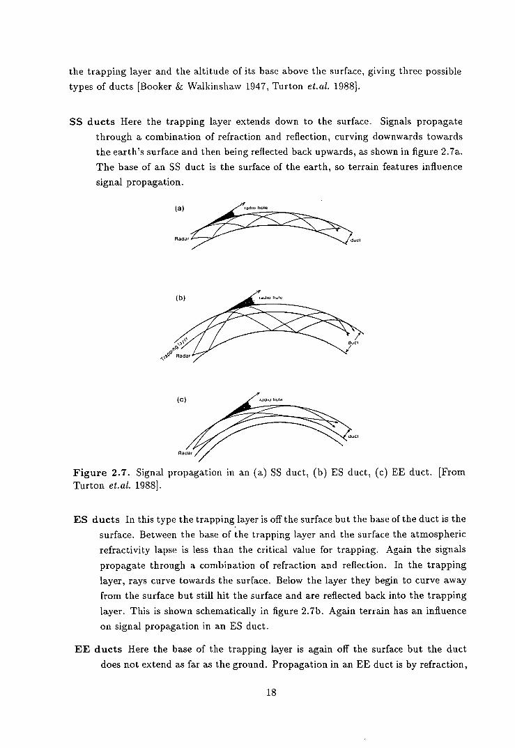
SS ducts Here the trapping layer extends down to the surface. Signals propagate
through a combination of refraction and reflection, curving downwards towards
the earth's surface and then being reflected back upwards, as shown in figure 2.7a.
The base of an SS duct is the surface of the earth, so terrain features influence
signal propagation.
(a) radio hole
:::4, dull
(C) ad.. I,k,
Raa,
auCt
Figure 2.7. Signal propagation in an (a) SS duct, (b) ES duct, (c) EE duct. [From Turton et.al . 19881.
ES ducts In this type the trapping layer is off the surface but the base of the duct is the
surface. Between the base of the trapping layer and the surface the atmospheric
refractivity lapse is less than the critical value for trapping. Again the signals
propagate through a combination of refraction and reflection. In the trapping
layer, rays curve towards the surface. Below the layer they begin to curve away
from the surface but still hit the surface and are reflected back into the trapping
layer. This is shown schematically in figure 2.7b. Again terrain has an influence
on signal propagation in an ES duct.
EE ducts Here the base of the trapping layer is again off the surface but the duct
does not extend as far as the ground. Propagation in an EE duct is by refraction,
18
with rays in the trapping layer being curved towards the surface and then being
curved back into the trapping layer but the more 'normal' refractivity conditions
below the base of the trapping layer. This is shown schematically in figure 2.7c.
Since an EE duct is not resting on the surface, terrain has no effect on signal
propagation.
The nomenclature for the three types of duct comes from one of the earliest works on
radio-meteorology [Booker & Walkinshaw 1947]. The letters refer to whether the base
of the trapping layer and duct are elevated or rest on the surface:
. SS duct: surface layer, surface duct
. ES duct: elevated layer, surface duct
. EE duct: elevated layer, elevated duct
This notation appears considerably simpler than the 'simple surface duct', 'surface S-
shaped duct' and 'elevated duct' used in more recent works [e.g. Hall 1979, DNOM
1984, Turton et.al. 1988].
Associated with ducting is the phenomenon of layer reflection. This occurs when there
is an extremely strong refractivity lapse (of hundreds of N-units/km). The layer acts
as a 'radio mirror', reflecting rays off it. This can be considered as an extreme form of
ducting, and will not be considered further in this work but is discussed in the various
works on propagation mentioned earlier.
The diagrams showing duct propagation make it clear that not all signals are trapped
in the duct. Trapping depends on the angle of elevation of the ray from the horizontal,
either when launched (if it starts within the duct) or when it enters the duct. The
critical angle at which rays begin to be trapped is a function of the thickness of the
duct and of the trapping layer [Dougherty & Hart 1979, Hall 1979 p32] and is found
in practice to be < ±0.5° [ibid.]. As well as the critical angle, there is also a critical
wavelength for trapping [Hall 1979 p30, Turton et.al .1988]
In a duct, signals are effectively trapped in two dimensions rather than three, so the
theoretical signal strength decreases inversely with range, rather following the inverse
square law of normal propagation [Hail 1979 p32]. Signal ranges are greatly enhanced,
e.g. the radar echoes from objects several thousand kilometres distant mentioned by
Durst [1947].
19
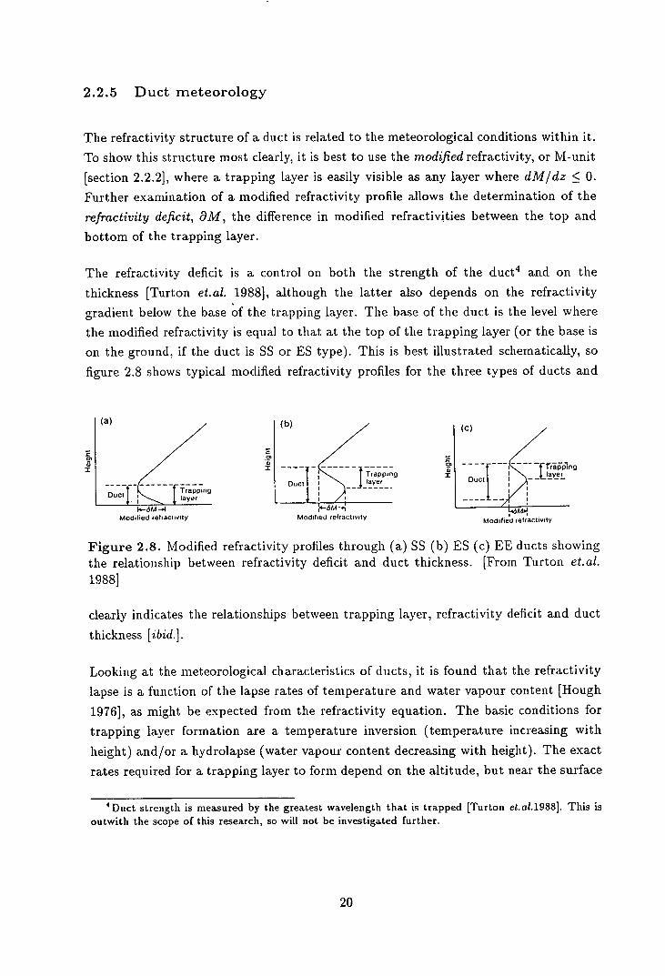
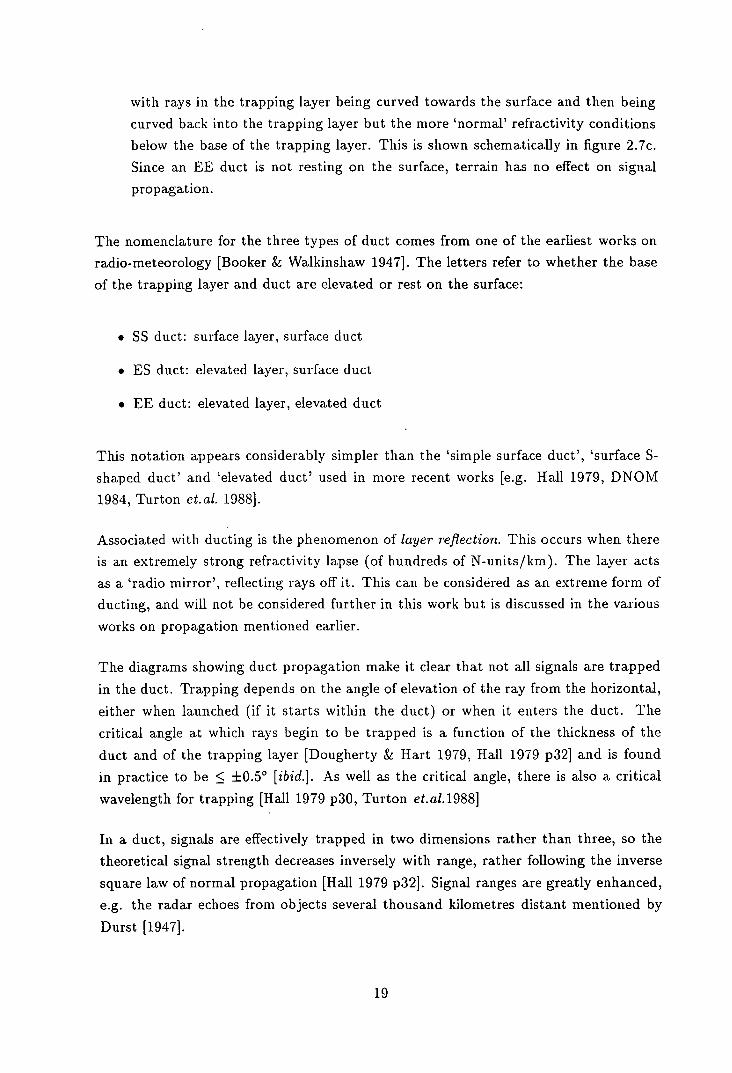
2.2.5 Duct meteorology
The refractivity structure of a duct is related to the meteorological conditions within it.
To show this structure most clearly, it is best to use the modified refractivity, or M- unit
[section 2.2.21, where a trapping layer is easily visible as any layer where dM/dz < 0.
Further examination of a modified refractivity profile allows the determination of the
refractivity deficit, OM, the difference in modified refractivities between the top and
bottom of the trapping layer.
The refractivity deficit is a control on both the strength of the duct 4 and on the
thickness [Turton et.al. 1988], although the latter also depends on the refractivity
gradient below the base of the trapping layer. The base of the duct is the level where
the modified refractivity is equal to that at the top of the trapping layer (or the base is
on the ground, if the duct is SS or ES type). This is best illustrated schematically, so
figure 2.8 shows typical modified refractivity profiles for the three types of ducts and
C Or a, I
(b) I(C)
C a 1 oJJ
u
Trapping
1EL Modified refractivity Modified refractivity Modified refractivity
Figure 2.8. Modified refractivity profiles through (a) SS (b) ES (c) EE ducts showing the relationship between refractivity deficit and duct thickness. [From Turton et.al.
1988]
clearly indicates the relationships between trapping layer, refractivity deficit and duct
thickness [ibid.].
Looking at the meteorological characteristics of ducts, it is found that the refractivity
lapse is a function of the lapse rates of temperature and water vapour content [1-lough
1976], as might be expected from the refractivity equation. The basic conditions for
trapping layer formation are a temperature inversion (temperature increasing with
height) and/or a hydrolapse (water vapour content decreasing with height). The exact
rates required for a trapping layer to form depend on the altitude, but near the surface
'Duct strength is measured by the greatest wavelength that is trapped [Turton et.ol.1988]. This is outwith the scope of this research, so will not be investigated further.
20
a trapping layer will form if [Hough 1976]:
UT ~ +0.087Km' (2.12)
az c9 r
< ~ —O .0F6gkg 1 m 1 (e rp) (2.13) az
If both the temperature and the moisture change, we find that the critical conditions
for trapping layer formation become:
1 O lOr (2.14)
where c and /3 are the critical gradients defined in equations 2.12 and 2.13 respectively
[ibid.].
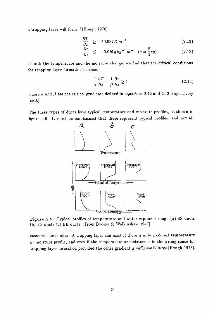
The three types of ducts have typical temperature and moisture profiles, as shown in
figure 2.9. It must be emphasised that these represent typical profiles, and not all
C
—Temperature
t Te .e t) TcrnPaj
—Potential Teinperal
I i)eficii DefcI!
L H... —peirii IIumid1't
ure-
I 1himitht tiff
Figure 2.9. Typical profiles of temperature and water vapour through (a) SS ducts (b) ES ducts (c) EE ducts. [From Booker & Walkinshaw 19471.
cases will be similar. A trapping layer can exist if there is only a correct temperature
or moisture profile, and even if the temperature or moisture is in the wrong sense for
trapping layer formation provided the other gradient is sufficiently large [Hough 1976].
21
2.3 Radio-meteorology
So far we have discussed ducts and the atmospheric conditions within them. It is now
time to turn our attention to the meteorological processes which give rise to ducts or
super-refractive layers. There are five major causes of ducts:
. Subsidence
. Offshore Advection
. Sea breezes (onshore advection)
. Nocturnal radiation
• Evaporation
This section will examine each mechanism briefly, giving key references where further
details may be found. The survey is made from a radio-meteorological point of view, all
five features are well understood meteorologically. Throughout the discussion, reference
will be made to ducts resulting from each process, but it should be understood that
the same conditions that lead to ducts also lead to super-refractive layers (SRLs) and
that both can be a cause of anaprop.
2.3.1 Subsidence
The meteorology of subsidence has been well understood for some time and is discussed
in many works [e.g. Namias 1933, McIntosh & Thom 1981 p144, Mcllveen 1986 p364].
The process basically involves the descent of cold, very dry air from near the tropopause.
As it descends, the air warms 5 . While the air subsides the mixing ratio (moisture
content) of the air hardly changes, resulting in a warm and dry air parcel near the
surface. Air below the base of the subsiding parcel is generally well mixed, moist and
cool relative to the subsiding air. At the boundary between the two, there is both a
temperature inversion and a hydrolapse, exactly the conditions that lead to a trapping
layer forming. Temperature and moisture changes can be very sharp, for example
a radiosonde ascent (Hemsby, 12Z, 18/8/78) showed a la/er 20 mb ( 200m) thick
exhibiting a temperature change of +5.6°C and a mixing ratio change of —4.1g kg'
[DAR 19781, giving a refractivity lapse rate of approximately 1.25 N-units/km.
'Descending air warms at the dry adiabatic lapse rate (9.8' C km - ') less the effects of radiational cooling (1-2°Cday 1 ).
22
The height of the interface (the subsidence inversion) varies on daily and seasonal
scales. At night, when convection in the boundary layer ceases, the inversion descends,
sometimes to as low as 500m, reaching a minimum at dawn. During the day it ascends,
reaching a maximum altitude at dusk [Bye 1988a]. The maximum altitude depends
very much on the type of surface and factors such as the amount of cloud cover and
the temperature. On a seasonal scale, inversions are generally higher in summer than
in winter [Bali 1960] since hotter surfaces give a greater depth of convection.
Subsidence ducts are almost always of the EE type [Gossard 1981], giving anaprop over
the entire area of subsidence. Subsidence is one of the most important mechanisms
causing interference.
2.3.2 Offshore Advection
In meteorology, advection is defined as "the horizontal transport (of heat, mass etc.)
effected by the horizontal exchange of air" [Mdllveen 1986 p4311. Like subsidence, it
is a well-understood phenomenon [ibid., McIntosh & Thom 1981 p94]. The form of
advection that is of particular interest to radio-meteorologists is the advection of air
offshore from land to sea.
When warm, dry air is advected offshore over a relatively cool sea, the lowest layers
are cooled by the evaporation of moisture into them [Turton et.al. 1988]. This leads
to, at the top of the modified layer, a temperature inversion and a hydrolapse, the
optimum conditions for the formation of a trapping layer. An advection duct is also
possible when cold, dry air is advected over a warmer sea. Here evaporation produces
a hydrolapse strong enough to overcome the effects of the temperature gradient and
cause super-refraction or trapping [Hough 1976]. In both cases, the resulting duct is of
the SS type or occasionally of the ES type [DNOM 1984].
Both the thickness and offshore extent of the advection duct are subject to debate.
The average thickness has been suggested to be as little as 25 metres [Hall & Barclay
1989 p159] or as much as 150 metres [Gough 1984, COST 19911. It is clear that the
thickness varies with distance offshore, building up to a maximum some 100 km from
the coastline, then decreasing slowly [DNOM 1984]. This profile has been modelled
for various parts of the world [Gossard 1982, Ko et.al. 1983, Garrett 1987, Garrett &
Ryan 1989]. The extent of the duct has been said to be between 50-200 km [DNOM
1984, Turton et.al.1988] and 1000 km [Bye 1988a], obviously depending on the size of
the sea area. It appears that the strength of the advection duct decreases with distance
offshore [DNOM 1984, COST 1991].
23
Advection ducts are not as effective at trapping signals as subsidence ducts, so they do
not give rise to such high signal levels as subsidence ducts [Bye 1988a].
2.3.3 Sea breeze advection
The sea breeze is a circulation set up when the land surface is at a greater temperature
than the sea. This results in a heat low overland and a low level flow from sea to
land [McIntosh & Thom 1981 p140]. This flow brings cool, moist air from sea to land,
undercutting the warmer, drier overland air and giving the ideal conditions for ducting.
Moisture gradients are particularly strong at the interface between sea and land air.
The sea breeze occurs during the day, building up as the land heats and reaching a
maximum in the late afternoon and early evening. Since the land must be warmer than
the sea for the circulation to develop, the sea breeze is more common in summer than
in winter.
The sea breeze flow is fairly shallow, only a few hundred metres thick [Mdllveen 1986
p289] so any radio ducts would be at low levels and so could have severe effects on
surface paths, and can penetrate some distance inland. Simpson et.al. [1977], studying
the sea breeze on the south coast of England, suggest that the sea air can regularly
penetrate over 40 km inland, even over the hilly terrain of the South Downs and
occasionally penetrates as far as 100 km inland. The inland penetration depends on
the relative temperatures of the land and sea surfaces [ibid.] as well as on any larger
scale air movements [Pearson et.al. 1983].
The association of the sea breeze with ducting was identified in the 1940's. Hatcher &
Sawyer [1947], using measurements made from aircraft near Madras, India, suggest a
radio duct about 1000 feet (300 m) thick, penetrating up to 15 miles (25 km) inland
during sea breeze conditions, but no indication of the strength of the duct is given.
The current Royal Navy document on radio-meteorology [DNOM 19841 suggests similar
thicknesses and inland penetrations, pointing out that the inland penetration will be
greater in low latitudes where sea breezes are more pronounced and that the sea breeze
duct will occur mainly in the afternoon and early evening, when the sea breeze is most
developed. An interesting observation is that the sea breeze duct extends offshore as
well as onshore. This could be of importance where there is no advection. Bye [1988a]
considers the sea breeze as an onshore extension of the advection duct, penetrating
some 30 to 40 km inland over flat terrain.
Although not studied in detail elsewhere in this work, the author feels that there are
problems with the existing treatment of the sea breeze by radio-meteorologists. Some
24
comments and suggestions for further work are made in the conclusions of this thesis
[Chapter 71.
2.3.4 Nocturnal radiation cooling
At night, if the sky is clear, the land surface will lose heat very rapidly through long-
wave radiation to space. This process, nocturnal radiation cooling, can cause anaprop
on land and coastal signal paths. The meteorology of nocturnal radiation cooling is well
understood [e.g. McIntosh & Thom 1983 p291 and the association with anaprop has
been recognised since the 1940's [e.g. Smith-Rose & Stickland 1947, Bean & Dutton
1966 p1331.
As the land surface cools, the lowest layers of the atmosphere will also cool and, if the
wind is sufficiently light to inhibit turbulent mixing, a low level temperature inversion
will form at the top of the cooled layer [Lochtie 1985]. There may also be a moisture
inversion, since water will condense out of the cooled air as it becomes saturated, but
this will depend on the initial moisture content and on the degree of cooling. If moisture
does condense out, the heat released will decrease the strength of the temperature
inversion, inhibiting the strength of the refractivity lapse.
The existence of a duct will depend on the strength of the temperature inversion and
the presence or absence of a moisture inversion [Hall 1979 p34]. The extent of a duct
will depend on the local topography, with 'pools' of super-refractivity trapped in areas
of flat ground [Bye 1988a]. A radiation duct will be strongest at the end of the night,
when the surface temperature is lowest, but may cause more severe anaprop shortly
after dawn, when convection is strong enough to lift the super-refractive layer above
the surface but not yet strong enough to destroy it [ibid.].
As part of their research into radio-meteorology, BTL considered ways of predicting
'radiation nights' from meteorological data [Lochtie 19851. Their criteria were:
• Little or no cloud cover throughout the night.
• Calm or light winds throughout the night.
• Dry air (R.H. less than 90%).
• High pressure.
Using computer analysis of surface observations, BTL were able to correctly 'predict'
25
about 80% of radiation nights identified on synoptic charts. Such analysis was consid-
ered a potential means of forecasting anaprop from meteorological data, but interest
in such work appears to have diminished in recent years.
2.3.5 Evaporation ducts
The four causes of ducting that have already been considered have been directly related
to synoptic scale weather systems. There is another ducting mechanism which has
been observed worldwide [Turton et.al . 19881 and can cover even larger areas than
the advection and subsidence ducts within anticyclones. These are Evaporation Ducts
which occur over water surfaces, not only the seas and oceans but also over large lakes.
As the name suggests, the ducts are formed by evaporation from the water surface
creating a saturated layer at the surface with unsaturated air a few metres up. The
resulting hydrolapse can be strong enough to allow a duct to form. The duct is an SS
type, and is only a few metres thick, showing complex diurnal, seasonal and geograph-
ical variations [DNOM 1984]. Average thickenesses are about 5m in the North Sea
[Rotherham 19741 and about 15m in the Mediterranean and Caribbean Seas [Turton
et.al . 1988]. Despite their small vertical extent, evaporation ducts can extend over
the entire open water surface so trapped signals are able to propagate far beyond the
radio horizon. The meteorology and radio-meteorology of the evaporation duct has
been investigated by a number of workers, including Hall & Gardiner [1968], Hamilton
& Laevastu [1973], Rotherham [1974], Gossard [1981] and Hall & Barclay [1989].
Evaporation ducts will be thickest under clear skies, during the day [Hall & Barclay
1989]. If the sea is warmer than the surface air there will be a continual upwards flux
of water vapour, thus reducing the strength of the duct [Hamilton & Laevastu 19731.
If there is an 'inversion' with warm air over a cooler sea (which can occur in regions
of upwelling or when warm air is advected offshore) the duct will be thicker. It is
suggested [Cossard 1981] that the thickness of the evaporation duct depends primarily
on atmospheric stability.
2.4 The radio-meteorology of anticyclones
It has been known for more than half a century that most cases of severe anaprop are
associated with anticyclones. This section looks at the relationship between anticy-
clones and anomalous propagation, starting with an examination of the evidence for
26
the relationship. This is followed by a brief examination of the meteorology of anticy-
clones and finally by an examination of a recently produced conceptual model of the
radio-meteorology of anticyclones.
2.4.1 Anticyclones and anaprop
Although the influence of atmospheric conditions on radio signals was identified during
the 1920's [Appleton 1947], it was not until the extensive use of radar during World War
II that the scale and severity of the problem was studied. It was quickly recognized that,
in Europe at least, the majority of anaprop occurred during anticyclonic conditions.
In the first ever conference on radio-meteorology, Appleton [ibid.] gave examples of
greatly increased radar ranges and noted that they were due to advection, nocturnal
radiative cooling and subsidence associated with high pressure systems. Smith-Rose &
Stickland [1947] noted the effects of radiative cooling as a cause of high signal levels on
land paths and also observed that the majority of enhanced signal levels on both land
and sea paths occurred during anticyclonic conditions. Johnson [1947] noted the effects
of temperature inversions, particularly those due to anticyclonic subsidence, on signals
while Alexander [1947] observed that advection of warm air offshore in the circulation
of a high gave increased ranges, even when the subsidence inversion was very weak.
Studies of anaprop over the Arabian Sea (where anomalous radar ranges of several
thousand kilometres had been observed, noted the effects of advection and the sea
breeze [Durst 1947, Booker 19481. Booker & Walkinshaw [1947], as well as making one
of the first detailed studies of ducts, noted that the majority of ducts occurred during
anticyclonic conditions and mentioned subsidence and nocturnal radiative cooling as the
causes. Booker [1948] stated that anticyclonic subsidence was linked to the majority
of anaprop, both directly and indirectly as an indicator of advection and nocturnal
cooling.
In the 1960's, Flavell [1964] noted anaprop was often due to the descent of the sub-
sidence inversion during anticyclonic conditions, while Bean & Dutton [1966 p132-41
consider advection, radiative cooling during anticyclones and anticyclonic subsidence
to be main meteorological processes responsible for ducts. Kuhn & Ogulewicz [1970]
note that the majority of anaprop they observed was caused by temperature inversions
within anticyclones. Hough [1976] and Muihearn [1976] give advection, anticyclonic
subsidence and nocturnal radiative cooling as the meteorological conditions associated
with ducting and Flavell [1978] again notes the importance of subsidence within anti-
cyclones as a cause of long-range propagation, as does Hail [1979], although the latter
author's meteorology is sometimes suspect. The importance of subsidence, nocturnal
27
radiative cooling and advection, all associated with anticyclones, is stressed many times
during the 1980's and early 90's [Hewitt & Adams 1980, Gossard 1981, Flavell 1981,83,
DNOM 1984, Clow 1984, Lochtie 1985, Juy & Spillard 1988, Turton et.al. 1988, Bye
1988a,b, Hall & Barclay 1989, Spillard 1989a,b, 1991, COST 1991].
From the above, it is clear that a great deal of anaprop occurs during anticyclonic
conditions, through the processes of subsidence, advection and nocturnal radiative
cooling. Models have been developed to show how these mechanisms occur within
anticyclones. Before these models are examined, it is useful to look briefly at the
meteorology of anticyclones.
2.4.2 The meteorology of anticyclones
Anticyclones are the weather systems associated with regions of high pressure and, in
the northern hemisphere, air flowing clockwise about the centre of the high. They are
generally areas of fine and settled weather, with light winds. Anticyclones come in two
main types - cold, or polar, highs and warm, or dynamic, highs, depending on the
temperature in the lower troposphere. The type of most interest to radio-meteorologists
is the warm anticyclone [Bye 1988a].
A warm high has a column of subsiding air from the tropopause to the top of the
boundary layer, with convergence aloft and divergence below to maintain continuity.
At the start of its descent the subsiding air is cold and very dry, so warms at the dry
adiabatic lapse rate of 9.8°Ckm 1 , modified by radiative cooling of about 2°C per
day. Since there is little mixing, the descending air does not gain moisture, so is hot
and dry as it reaches low levels. This contrasts sharply with the well mixed air in the
boundary layer which is both cool and moist relative to the subsiding air. The result
is a temperature inversion and a strong hydrolapse, the subsidence inversion discussed
above.
The subsidence inversion, and therefore the associated super- refractive layer, is dome-
shaped [Namias 1933], with the highest point over the place where the rate of increase
in surface pressure is greatest [ibid.], not centred over the highest surface pressure as
some works [e.g. Bye 1988a] suggest. The subsiding air descends in a clockwise spiral,
taking several days over the descent, and the mean flow below the subsidence inversion
is also clockwise, turned slightly away from the high pressure centre by friction. This
flow is the advection described in the previous section.
Because of the overall descent and the presence of the subsidence inversion, the growth
of convective clouds is limited, so clouds will be stratiforrn if present. In the latter case,
the clear skies allow radiative cooling at night and the formation of radiation ducts.
This very superficial examination of anticyclones has shown that three of the main
causes of anaprop are linked to them. The place of the mechanisms in an anticyclone
has been studied in detail by radio-meteorologists at BTL and a conceptual model of
a high has been developed.
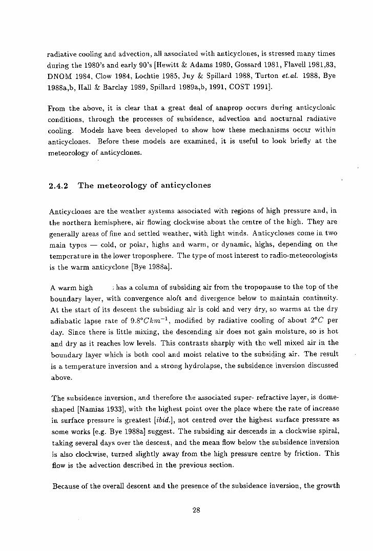
2.4.3 The BTL anticyclone model
As part of their ongoing research into anaprop, BTL have produced a conceptual model
of an anticyclone, together with predictions of the anaprop it produces. The model [Bye
1988a, COST 1991 A2.41 looks at a warm anticyclone in summer as the high pressure
centre develops and moves over the UK and then across the southern North Sea. The
meteorology of the model is shown in figure 2.10, which shows the situation during
converging air in converging the tropopause
air in the
t tropopause 4P 4P
tj air in low ascending I air subsiding )t
..— ascending
air in tow air subsidin_$ pressure 4-.. and warming
pressure ( and warmin
system
system general clockwise
— general clockwise 9 circulation of
J circulation — anticyclone
ir anticyclon
9 divergence of air
divergence of air at tow levels - 4 at low levels a
inversion level
/ - A inversion level S_Sb
A A"G . A convection &
is
o a C turbulent mixing
- at night
A
surface radiation
A C tQ at the surface
a S.f Cv
advection from the continent advection from the continent
Figure 2.10. The meteorology of the BTL anticyclone model (a) during the day and (b) during the night. [From Bye 1988a]
the day and during the night. At all times the picture is dominated by the overall
subsidence and the general clockwise circulation advecting air from the continent over
the southern North Sea and UK mainland. During the day, there is convection above
29
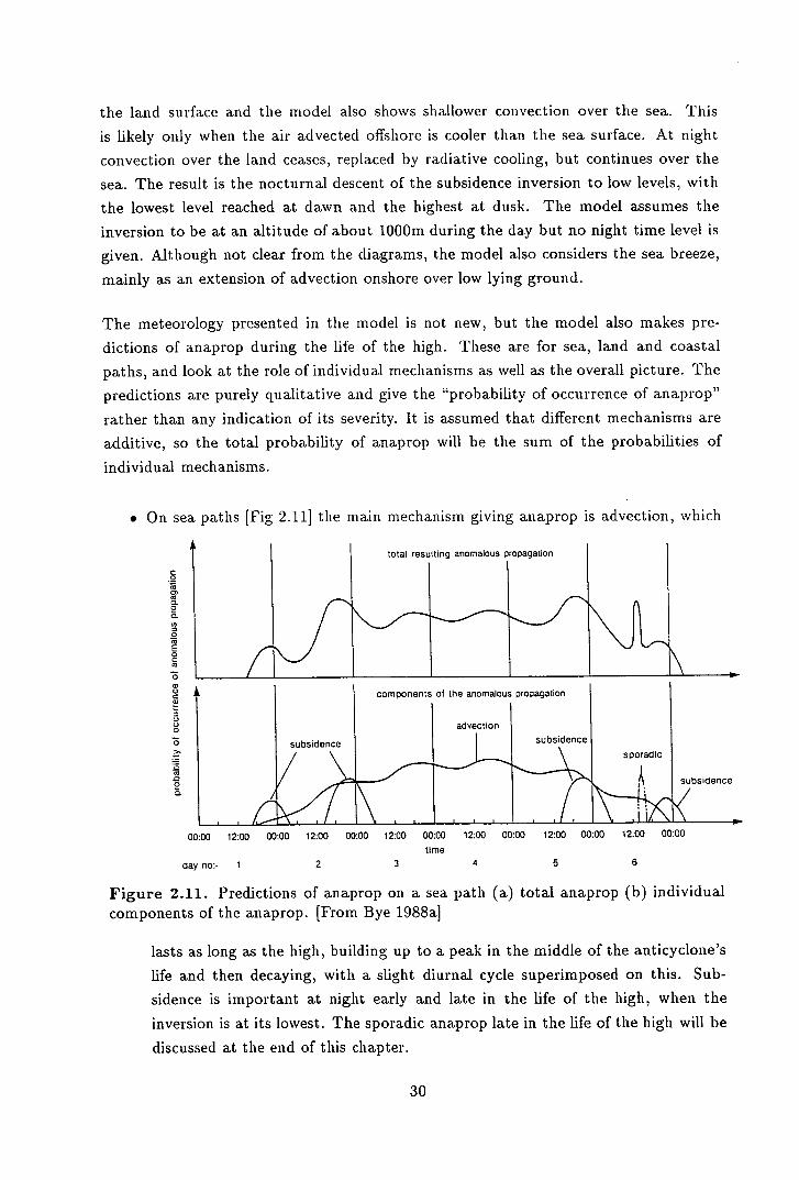
the land surface and the model also shows shallower convection over the sea. This
is likely only when the air advected offshore is cooler than the sea surface. At night
convection over the land ceases, replaced by radiative cooling, but continues over the
sea. The result is the nocturnal descent of the subsidence inversion to low levels, with
the lowest level reached at dawn and the highest at dusk. The model assumes the
inversion to be at an altitude of about 1000m during the day but no night time level is
given. Although not clear from the diagrams, the model also considers the sea breeze,
mainly as an extension of advection onshore over low lying ground.
The meteorology presented in the model is not new, but the model also makes pre-
dictions of anaprop during the life of the high. These are for sea, land and coastal
paths, and look at the role of individual mechanisms as well as the overall picture. The
predictions are purely qualitative and give the "probability of occurrence of anaprop"
rather than any indication of its severity. It is assumed that different mechanisms are
additive, so the total probability of anaprop will be the sum of the probabilities of
individual mechanisms.
On sea paths [Fig 2.11] the main mechanism giving anaprop is advection, which
0
ci C, Co 0 0 0
S 0
C 0 C a
0 a U C a,
S U C-, 0
0
Ca
0
a
4' I I components of the anomalous propagation I I
advection
subsidence I I I I subsidence
sporadic
subsidence
00:00 12:00 00:00 12:00 00:00 12:00 00:00 12:00 00:00 12:00 00:00 12:00 00:00
time
day no:- 1 2 3 4 5 6
Figure 2.11. Predictions of anaprop on a sea path (a) total anaprop (b) individual components of the anaprop. [From Bye 1988a]
lasts as long as the high, building up to a peak in the middle of the anticyclone's
life and then decaying, with a slight diurnal cycle superimposed on this. Sub-
sidence is important at night early and late in the life of the high, when the
inversion is at its lowest. The sporadic anaprop late in the life of the high will be
discussed at the end of this chapter.
Ku]
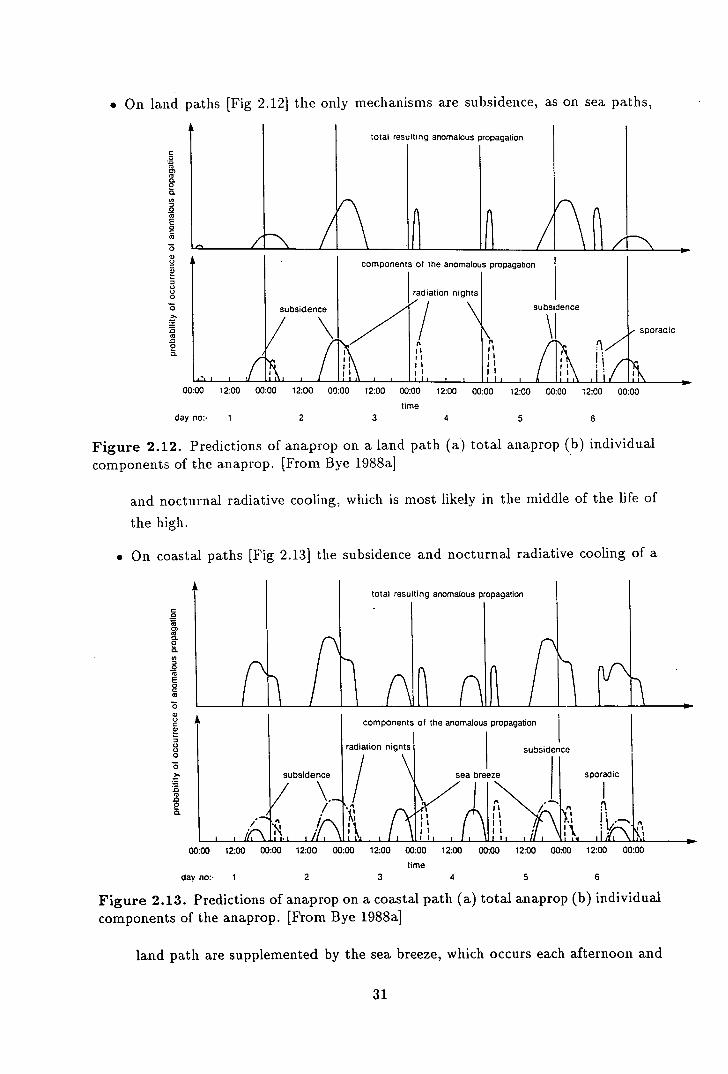
On land paths [Fig 2.12] the only mechanisms are subsidence, as on sea paths,
total resulting anomalous propagation
C 0
a 0) C, 0. 0 0.
0 0 'a E 0 C 'a
0 a U C a,
a, U
components of the anomalous propagation
U radiation nights I 0
subsidence ubsidence
/ \ 1 sporadic a
2 0.
II II
00:00 12:00 00:00 12:00 00:00 12:00 00:00 12:00 00:00 12:00 00:00 12:00 00:00
time
day no:- 1 2 3 4 5 6
Figure 2.12. Predictions of anaprop on a laud path (a) total anaprop (b) individual components of the anaprop. [From Bye 1988a]
and nocturnal radiative cooling, which is most likely in the middle of the life of
the high.
. On coastal paths [Fig 2.131 the subsidence and nocturnal radiative cooling of a
components of the anomalous propagation
radiation nights subsidence
subsidence / sea breeze
\._ /
sporadic
0. I
/I
/
I . II \i I lii i i/i
00:00 12:00 00:00 12:00 00:00 12:00 00:00 12:00 00:00 12:00 00:00 12:00 00:00
time
day no:- 1 2 3 4 5 6
Figure 2.13. Predictions of anaprop on a coastal path (a) total anaprop (b) individual components of the anaprop. [From Bye 1988a]
land path are supplemented by the sea breeze, which occurs each afternoon and
C 0
a CI a 0. C 0. 'a a, 0 M
E 0 C a
0 a, U C a,
a, U U 0
0 >.
M
31
early evening.
As part of the work for this project, the author made an examination of the BTL
model. This study [Jones 19891 looked at the meteorology behind the model and made
case studies of actual periods of anticyclonic anaprop which were compared with the
predictions given by the model. It was found that the model was generally good,
although mixed paths caused problems and some signals were observed at times when
the model predicted none. These were not considered important as the model gave the
probability of anaprop rather than signal levels. The study also suggested ways that
the model could be extended to consider anticyclones north, south and west of the UK
and in winter as well as in summer.
2.5 The radio-meteorology of fronts
Fronts have not been particularly well studied from a radio-meteorological point of
view, although they have been the target of a great deal of meteorological research. An
important objective of this thesis is to remedy this discrepancy, and apply some of the
current meteorological understanding of fronts to their radio- meteorology.
This section will look at two aspects of the radio-meteorology of fronts. The first is
the current understanding of the behaviour of radio signals at and near fronts. The
second is a particular problem which has been termed sporadic subsidence, which was
identified in the early 1980's as a cause of particularly severe anaprop at some fronts.
There will not be a detailed examination of the meteorology of fronts. Such a study
could easily fill several volumes, and is outwith the scope of this research. The most
important references on fronts are given in chapter 4, where the current meteorological
models are applied to the problem of frontal anaprop.
2.5.1 Fronts and anaprop
That fronts have an effect on radio signals has been known for nearly half a century.
Smith-Rose & Stickland [1947] mention 'disturbances' in signal levels as fronts cross a
sea path off Wales, but they note that "at present these cases are difficult to predict
since the effect is by no means uniform". They also note problems caused by the lack
of detailed meteorological data over the path, a mournful cry that will be heard many
times in the course of this work. Later in their paper, they state that signal levels
decrease as a warm front passes, remain low in the warm sector and then rise sharply
as the cold front passes.
Observations made in New Zealand from 1943-45 also indicated that depressions have
an effect on signals, with 'unexpectedly long' radar ranges reported when the radar
beam was pointing along the length of a trough [Alexander 19471. The paper noted,
however, that ranges in other directions could not be checked due to an absence of
radar targets! In the USA, Randall (1947, cited by Bean & Dutton [1966 p176]) also
observed signal strength changes when a cold front crossed a signal path, with high
signal levels before the front arrived, then a rapid fall as the surface front reached the
path.
Bean & Dutton [1966 p185-95] made a theoretical study of the refractivity structure of
warm and cold fronts, using the 'Bergen' model of frontal structure [Chapter 4]. This
work, although significant in that it was the first such study, sheds little light on the
problem of anaprop at fronts. A close examination reveals that the main aim of Bean
& Dutton's work was to show how different refractivity units highlighted the discon-
tinuity between different air masses at the frontal zone. A further study by the same
authors [Bean & Dutton 1966 p195-2111 uses real data, but concentrates on variations
in the horizontal refractivity structure at different levels with no consideration of the
potential for anaprop at the fronts. A final study [ibid. p212-223] looked at the vertical
refractivity structure, both in time and space, through a cold front as it crossed the
USA. The study again has no mention of super-refraction or the potential for anaprop,
but a close inspection of the figures shows a strongly super-refractive layer ahead of
and behind the front. The layer starts at an altitude of around 2000m, descends to
about 1000m just before the front, and then ascends (and weakens) behind the front
[ibid. p212].
The next reference to fronts comes from some research in Eastern Europe. Kuhn &
Ogulewicz [1970], studying a sea path over the Baltic, observed signal behaviour as
both warm and cold fronts passed. They found that, on average, passage of a warm
front was accompanied by an increase in signal level of some 30 dBf over a four hour
period while passage of a cold front was marked by a fall of some 25 dB?over a two
hour period. It should be noted that these represent the averages, and the authors were
careful to point out that not all fronts gave rise to such large changes in level [ibid.]. It
is also worth noting that the high signal levels in the warm sector are the opposite of
the earlier findings of Smith-Rose & Stickland [1947].
A number of references to the effects of fronts were made during the 1980's. Hewitt &
Adams [1980] mention weather froflts "cause significant enhancements" and that the
18
33
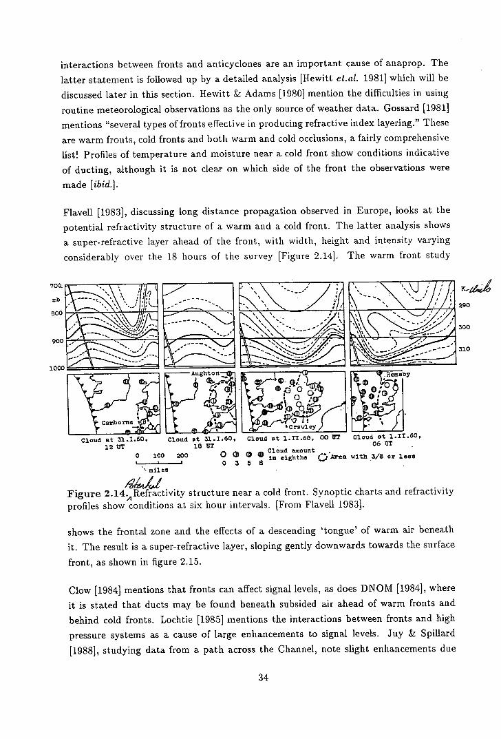
700.
inb
800
IVllaA! 900
1000 _ -
-I 01 M
290
300
310
interactions between fronts and anticyclones are an important cause of anaprop. The
latter statement is followed up by a detailed analysis [Hewitt et.al. 1981] which will be
discussed later in this section. Hewitt & Adams [1980] mention the difficulties in using
routine meteorological observations as the only source of weather data. Gossard [1981]
mentions "several types of fronts effective in producing refractive index layering." These
are warm fronts, cold fronts and both warm and cold occlusions, a fairly comprehensive
list! Profiles of temperature and moisture near a cold front show conditions indicative
of ducting, although it is not clear on which side of the front the observations were
made [ibid.].
Flavell [19831, discussing long distance propagation observed in Europe, looks at the
potential refractivity structure of a warm and a cold front. The latter analysis shows
a super-refractive layer ahead of the front, with width, height and intensity varying
considerably over the 18 hours of the survey [Figure 2.141. The warm front study
' 'e!nsby D '
AughtOTr1 II
o
'crw1ey
Cloud at 31.1.60, Cloud at 31.1.60, Cloud at 1.11.60, 00 T Cloud at 1.11.609
12 UT 18 UT - - 06 UT
?
100 200 in eighths Qea with .3/8 or less
' miles
A&e4ractivityFigure 2.14> structure near a cold front. Synoptic charts and refractivity profiles show conditions at six hour intervals. [From FlaveIl 19831.
shows the frontal zone and the effects of a descending 'tongue' of warm air beneath
it. The result is a super-refractive layer, sloping gently downwards towards the surface
front, as shown in figure 2.15.
Clow [1984] mentions that fronts can affect signal levels, as does DNOM [1984], where
it is stated that ducts may be found beneath subsided air ahead of warm fronts and
behind cold fronts. Lochtie [1985] mentions the interactions between fronts and high
pressure systems as a cause of large enhancements to signal levels. Juy & Spillard
[1988], studying data from a path across the Channel, note slight enhancements due
34
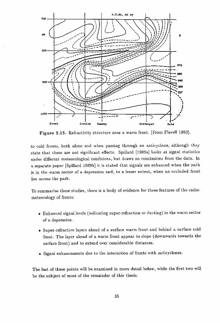
4.X.80, 00 UT
100_
ob
300—
_-
900-
000—
/ nr at ra1ey Heby Stavanger 0.1.
Figure 2.15. Refractivity structure near a warm front. [From Flavell 1983].
to cold fronts, both alone and when passing through an anticyclone, although they
state that these are not significant effects. Spillard [1989a] looks at signal statistics
under different meteorological conditions, but draws no conclusions from the data. In
a separate paper [Spillard 1989b] it is stated that signals are enhanced when the path
is in the warm sector of a depression and, to a lesser extent, when an occluded front
lies across the path.
To summarise these studies, there is a body of evidence for three features of the radio-
meteorology of fronts:
• Enhanced signal levels (indicating super-refraction or ducting) in the warm sector
of a depression.
• Super-refractive layers ahead of a surface warm front and behind a surface cold
front. The layer ahead of a warm front appear to slope (downwards towards the
surface front) and to extend over considerable distances.
• Signal enhancements due to the interaction of fronts with anticyclones.
The last of these points will be examined in more detail below, while the first two will
be the subject of most of the remainder of this thesis.
I
rio
280
290
,00
I-
t -1 1
35
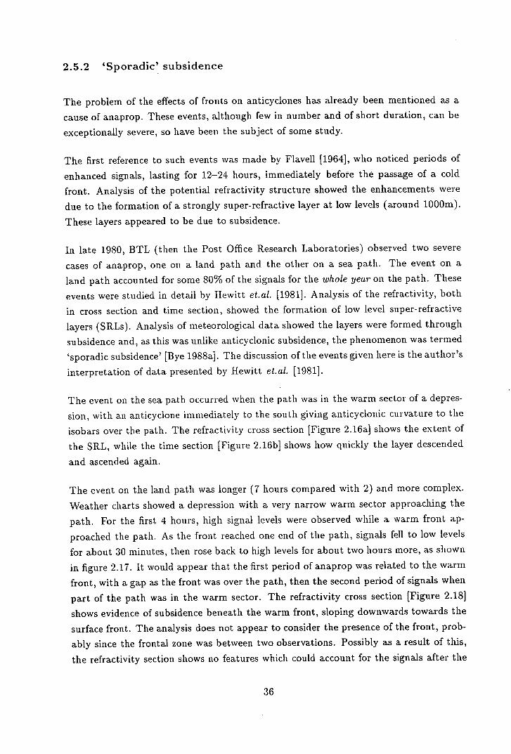
2.5.2 'Sporadic' subsidence
The problem of the effects of fronts on anticyclones has already been mentioned as a
cause of anaprop. These events, although few in number and of short duration, can be
exceptionally severe, so have been the subject of some study.
The first reference to such events was made by Flavell [1964], who noticed periods of
enhanced signals, lasting for 12-24 hours, immediately before the passage of a cold
front. Analysis of the potential refractivity structure showed the enhancements were
due to the formation of a strongly super-refractive layer at low levels (around 1000m).
These layers appeared to be due to subsidence.
In late 1980, BTL (then the Post Office Research Laboratories) observed two severe
cases of anaprop, one on a land path and the other on a sea path. The event on a
land path accounted for some 80% of the signals for the whole year on the path. These
events were studied in detail by Hewitt et.al. [1981]. Analysis of the refractivity, both
in cross section and time section, showed the formation of low level super-refractive
layers (SRLs). Analysis of meteorological data showed the layers were formed through
subsidence and, as this was unlike anticyclonic subsidence, the phenomenon was termed
'sporadic subsidence' [Bye 1988a]. The discussion of the events given here is the author's
interpretation of data presented by Hewitt et.al. [1981].
The event on the sea path occurred when the path was in the warm sector of a depres-
sion, with an anticyclone immediately to the south giving anticyclonic curvature to the
isobars over the path. The refractivity cross section [Figure 2.16a] shows the extent of
the SRL, while the time section [Figure 2.16b] shows how quickly the layer descended
and ascended again.
The event on the land path was longer (7 hours compared with 2) and more complex.
Weather charts showed a depression with a very narrow warm sector approaching the
path. For the first 4 hours, high signal levels were observed while a warm front ap-
proached the path. As the front reached one end of the path, signals fell to low levels
for about 30 minutes, then rose back to high levels for about two hours more, as shown
in figure 2.17. It would appear that the first period of anaprop was related to the warm
front, with a gap as the front was over the path, then the second period of signals when
part of the path was in the warm sector. The refractivity cross section [Figure 2.181
shows evidence of subsidence beneath the warm front, sloping downwards towards the
surface front. The analysis does not appear to consider the presence of the front, prob-
ably since the frontal zone was between two observations. Possibly as a result of this,
the refractivity section shows no features which could account for the signals after the
36
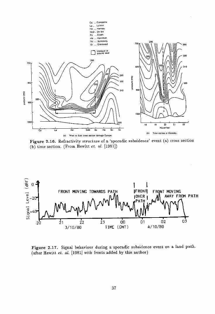
Ca .... Camoorno
La .....
He Hemsor
DeE.. Do Bit
Es ..... Essen
Ha ,... Hannover
Sc .... Sc#ieS'59
Dr .... GreilSWald
fl pressure at groUfla level
280
/
280
320 ,2 goo
290
300
n B
5, 0.
11 1000 [ 320 1 18 19 20 21 22
Ca La He DeE Es Ha Sc Or November
(b) Time section at Hemsby. (a) West to East cross section through Europe.
Figure 2.16. Refractivity structure of a 'sporadic subsidence' event (a) cross section (b) time section. (From Hewitt et. al. [19811)
I I IFRON11 FR NT MOVING JOVER AWAY FROM PATH
9 PATH K *fnA
di 62 6 4/10/80
Co 0 -c
FRONT MOVING TOWARDS PA Q.) > a.) -J
Co c —L
U.)
20 21 22 23 00
3/10/80 TIME (GMT)
Figure 2.17. Signal behaviour during a sporadic subsidence event on a land path.
(after Hewitt et. al. [1981] with fronts added by this author)
37
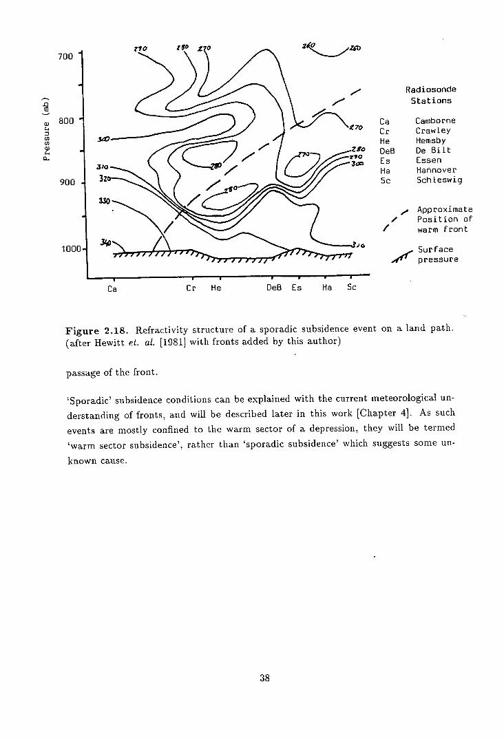
Ca C He DeB Es Ha Sc
800
CL
U) U) a)
700
.0 a
WX
1001
Radiosonde Stations
Ca Camborne Cr Crawley He Hemsby DeB De But Es Essen Ha Hannover Sc Schleswig
, Approximate / Position of
/ warm front
Surface .WK pressure
Figure 2.18. Refractivity structure of a sporadic subsidence event on a land path.
(after Hewitt et. al. [1981] with fronts added by this author)
passage of the front.
'Sporadic' subsidence conditions can be explained with the current meteorological un-
derstanding of fronts, and will be described later in this work [Chapter 41. As such
events are mostly confined to the warm sector of a depression, they will be termed
'warm sector subsidence', rather than 'sporadic subsidence' which suggests some un-
known cause.
M.
Chapter 3
Statistical analysis of weather
and anaprop
Most studies of radio propagation rely heavily on statistics to present results and to
support theories, and this work is no exception. Because most data are the result
of several months or even years of analysis, some form of statistical summary is the
most appropriate way of presenting them. Models of propagation processes are often
formulae, in terms of easily calculated parameters, to give a close approximation to the
observed statistical distribution of signals on paths of a given type.
What is exceptional about this work is that, rather than looking at the data for a
given path or group of paths over a given period, the data are first classified by the
meteorological conditions and then statistics produced. This allows the long term
effects of different weather conditions to be compared. This information is not only
important for this thesis, but also for end users, who can use this information to help
plan where paths should be built. Only one previous work [Spillard 1991] has made
an analysis based on weather conditions, and that is considerably more limited, both
in the number of weather types and in the range of signal paths used, than the one
presented here.
This chapter begins with a summary of the way signal statistics are normally presented
and some of the studies made in the past. This is followed by an examination of the
data available for this study and the schemes used to analyse it. The main results of
the analysis are then presented. For operational use, a portfolio of "Interference Data
Sheets" has been produced and supplied to BTL. These are discussed here, with the
entire portfolio given in Appendix A of this thesis. The chapter closes with a discussion
39
of the significance of the results.
3.1 Previous work
A great deal of research into radio-meteorology and anomalous propagation has been
carried out over the last half century, and many of the results have been statistical in
nature. The main reasons for this are that there is too much information for any other
form of non-selective analysis and that the main use of the information has been to
provide long-term summaries that can be used in network planning. This is reflected
in the published literature, which can be divided into statistical results and methods
of predicting signal statistics.
3.1.1 Statistical analyses
Statistical analyses date back to the earliest publications on radio-meteorology. Shep-
pard [1947] studied the relationship between signal strength and the refractivity gra-
dient, observing a direct connection between the two. Durst [1947] gave statistics of
radio ducts and correlated them with meteorological conditions for several parts of
the world while Alexander [1947] presented similar results for New Zealand. Bean &
Dutton [1966] give statistics of refractivity lapse rates and of surface refractivities over
much of the USA, as well as correlating signal strength with meteorological variables.
Much of their work was climatological in nature, and did not look at the effects of dif-
ferent types of weather. Hall & Corner [1969], examining data collected in the UK over
a three year period, studied the refractivity structure in the lowest 1000 metres and
correlated this to the temperature and moisture profiles, as well as examining seasonal
and diurnal patterns. Kuhn & Ogulewicz [1970] compared the results they observed
in the Baltic with predictions given by the CCIR as well as studying the seasonal dis-
tributions of refractivity and signal strength. Flavell [1978] presented the results of a
study of refractivity obtained from radiosonde observations, concentrating particularly
on seasonal variations, while Hewitt & Adams [1981] looked at diurnal variations and
at the length of anaprop events on paths in the UK and to the Netherlands.
As part of the COST 210 project a great deal of statistical data were gathered from
signal paths over the UK and north-western Europe. The bulk of the results are sum-
marised in the final report [COST 1991] but some interesting information is contained
in a number of the interim publications [Hewitt 1984, Lochtie 1985, Hewitt 1985a, 1987,
Hammond 1989, Diik & van Noort 19891. Bye & Howell [1989] made an interesting
40
study of the refractivity lapse rate from meteorological data and found considerable
differences between coastal and inland observations.
Of most interest to this work are the results obtained by Spillard [1989a,b, 1991]. Using
signal data from the COST 210 cross channel network and 'Daily weather report' charts,
the studies examined the behaviour of signals under different weather conditions. An
initial study of 10 weather types and one observation a day for 9 months [Spillard
1989b] suggested that most signals were observed when an anticyclone was centred to
the east of the path with moderate enhancements when the path was ahead of a warm
front or behind a cold front. As will be shown in the next chapter, these results are in
keeping with the meteorological models developed by this author. A more detailed work
[Spillard 19911 looked at 11 weather types, using a whole year of 6-hourly observations.
Further subdivision considered the origin of the air, temperature and cloud cover. The
results showed considerable variation between weather types and between subdivisions
of each type but in most cases each category has only a few tens of hours of data, not
enough for a valid statistical analysis. This is discussed in the work and it is suggested
that use of a longer period of data and less subdivision would make the results more
meaningful. Another limitation of Spillard's work is that data were limited to sea paths
only, rather than examining a mixture of path types.
3.1.2 Prediction methods
A number of methods have been developed to predict signal statistics from factoirsuch
as path length and type and transmission frequency. Most of these methods produce
a cumulative distribution of some sort, showing the percentage of the time that signals
are expected to exceed a particular level. Such works include Hewitt [1987, 1988b,c],
Spillard [1991] and COST [1991]. While of great importance to radio scientists, such
models are of little importance to this work.
3.1.3 Presentation of signal data
The works mentioned in the preceding sections contain a bewildering array of ways of
presenting signal statistics. Closer inspection shows that many are similar, with the
objects either of showing how signals behave on average over the course of time or how
much of the time signals are expected to exceed a given level.
The main method used to present signal statistics is the cumulative distribution or CD.
41
This is a curve showing what percentage of the time signals exceed a given level. The
time axis is logarithmic and will typically range from 100% to about 0.0001%, while
the signal level axis ranges from the receiver noise level to some suitable maximum.
CDs are used extensively in this work and examples can be seen later in this chapter.
It is often useful to examine diurnal or seasonal trends in signals and to make com-
parisons between levels. Such charts show either the percentage of total signals (at all
levels) in a given time band or the percentage of signals recorded at a particular level.
This sort of data are usually presented as a bar or line graph, sometimes accompanied
by some form of average to smooth the data [e.g. Hammond 1989]. Again such charts
are used extensively in this work and examples can be seen later in this chapter. Not
used here, but of importance to organisations such as BTL, are event duration charts.
These show the number of anaprop events for each of a number of durations. Differ-
ent signal levels may be shown for comparisons to he made. Such information is of
importance when planning signal networks.
3.2 Data analysis
During discussions with BTL early in this project, it transpired that little or no work
had been done on the statistics of signals under different weather conditions. Since this
project needed an indication of the scale of frontal anaprop, it was decided to make
a detailed statistical analysis of two or three years data, looking at the incidence of
anaprop under different weather conditions.
3.2.1 Selection of data
As BTL were a major contributor to the COST 210 project, they were able to make
large quantities of data available to the author. Signal data from paths in the COST
210 North Sea Network for the years 1986-8 were supplied, as were the corresponding
weather charts from the BTL library. 1986-8 was chosen since the signal data were the
most complete - more recent material was often off site or not fully transcribed onto
computers.
Due to some problems with the data for 1988 (mainly missing or corrupt data files, as
well as the amount of time required to process all the data), it was decided to limit
the analysis to the two years 1986-7 and only to look at signal paths within the UK
mainland or to the Netherlands. The table below [Table 3.1] shows the final set of
42
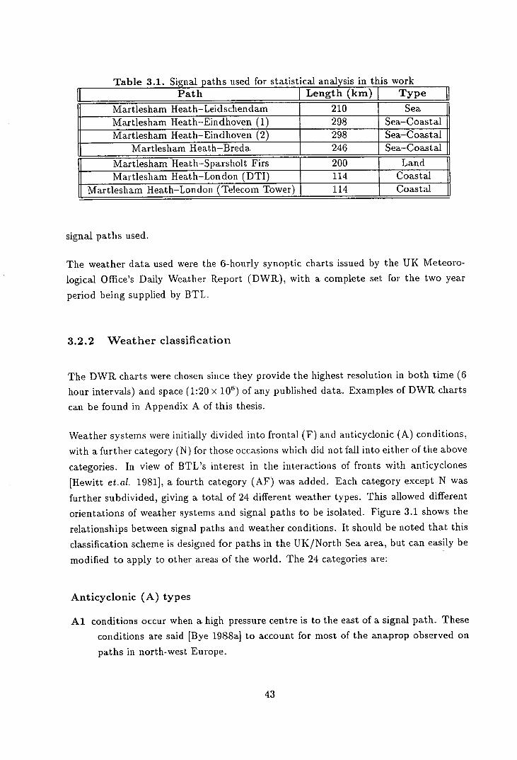
Table 3.1. Signal paths used for statistical analysis in this work Path I Length (km) I Type
Martlesham Heat h—Leidschendam 210 Sea Martlesham Heath—Eindhoven (1) 298 Sea—Coastal Martlesham Heath—Eindhoven (2) 298 Sea—Coastal
Martlesham Heath—Breda 246 Sea—Coastal
Martlesham Heath—Sparsholt Firs 200 Land Martlesham Heath—London (DTI) 114 Coastal
Martlesham Heath—London (Telecom Tower) 114 Coastal
signal paths used.
The weather data used were the 6-hourly synoptic charts issued by the UK Meteoro-
logical Office's Daily Weather Report (DWR), with a complete set for the two year
period being supplied by BTL.
3.2.2 Weather classification
The DWR charts were chosen since they provide the highest resolution in both time (6
hour intervals) and space (1:20 x 106) of any published data. Examples of DWR charts
can be found in Appendix A of this thesis.
Weather systems were initially divided into frontal (F) and anticyclonic (A) conditions,
with a further category (N) for those occasions which did not fall into either of the above
categories. In view of BTL's interest in the interactions of fronts with anticyclones
[Hewitt et.al. 1981], a fourth category (AF) was added. Each category except N was
further subdivided, giving a total of 24 different weather types. This allowed different
orientations of weather systems and signal paths to be isolated. Figure 3.1 shows the
relationships between signal paths and weather conditions. It should be noted that this
classification scheme is designed for paths in the UK/North Sea area, but can easily be
modified to apply to other areas of the world. The 24 categories are:
Anticyclonic (A) types
Al conditions occur when a high pressure centre is to the east of a signal path. These
conditions are said [Bye 1988a] to account for most of the anaprop observed on
paths in north-west Europe.
43
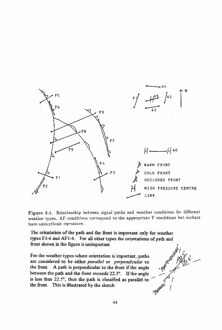
•-.. A 4
14fA2 V
f..JA6
) WARM FRONT
COLD FRONT
OCCLUDED FRONT
H HIGH PRESSURE CENTRE
LINK
Figure 3.1. Relationship between signal paths and weather conditions for different weather types. AF conditions correspond to the appropriate F conditions but isobars have anticyclonic curvature.
The orientation of the path and the front is important only for weather types Fl-6 and AF1-6. For all other types the orientations of path and front shown in the figure is unimportant.
V
For the weather types where orientation is important, paths are considered to be either parallel or perpendicular to the front. A path is perpendicular to the front if the angle between the path and the front exceeds 22.5°. If the angle is less than 22.5°, then the path is classified as parallel to the front. This is illustrated by the sketch:
q
44
A2 conditions are when the high pressure is centred to the west of a signal path.
A3 conditions occur when the high pressure centre is to the north of the signal path.
A4 conditions occur when the high pressure centre is to the south of the signal path.
A5 is when the high pressure is centred over or is very near to the signal path.
A8 conditions are when the path is between two highs, so pressures are higher at the
ends of the path than in the middle.
Frontal (F) types
Fl conditions occur when a cold front is 'perpendicular' to a signal path, that is,
moving along the path from one end to the other.
F2 conditions occur when a cold front is 'parallel' to a signal path, so the front moves
over the whole length of the path at once rather than moving from one end to
the other.
F3 corresponds to Fl conditions but for a warm front.
F4 corresponds to P2 conditions but for a warm front.
F5 corresponds to Fl conditions but for an occluded front.
F6 corresponds to F2 conditions but for an occluded front.
F7 conditions occur when a signal path cuts through the same front twice. The type
of front is unimportant.
F8 conditions occur when a path cuts both the warm and cold fronts of a single
depression, with the ends of the path ahead of and behind the warm sector.
F9 conditions occur when the entire path is in the warm sector of a depression and
isobars are either cyclonically curved or straight.
FO conditions are those where a path cuts two or more fronts, provided the weather
cannot be classified as P8.
Anticyclonic-Frontal (AF) types
AF1 corresponds to Fl but with anticyclonic curvature to the isobars.
AF2 corresponds to P2 but with anticyclonic curvature to the isobars.
AF3 corresponds to P3 but with anticyclonic curvature to the isobars.
AF4 corresponds to P4 but with anticyclonic curvature to the isobars.
45
AF5 corresponds to F5 but with anticyclonic curvature to the isobars.
AF6 corresponds to F6 but with anticyclonic curvature to the isobars.
AF9 corresponds to F9 but with anticyclonic curvature to the isobars.
unclassified (N) types
N covers cases where the large scale flow is cyclonic or linear, but there are no fronts
within about 100 km of the signal path. Any charts which cannot be classified
as A, F or AF are put into category N.
3.2.3 Verification of the weather classification scheme
The weather classification scheme was developed by meteorologists but was designed
to be used by non-professionals. To ascertain whether this was true, and to examine
the objectivity of the analysis, two tests were carried out. For the first, the author's
supervisor used the written classification guidelines [Jones 19901 to classify a two week
block of data. For the second, BTL were supplied with the same guidelines and were
asked to examine another two week block of data.
The first test provided a very good correlation between the two analysis, with 93%
(52/56 cases) of cases matching. The main differences were over whether some fronts
should be AF or F type, but it was felt that the scheme was objective and easy for a
meteorologist to use.
The second (BTL) analysis was less accurate, but still 84% (47/56) of cases agreed.
Again there were differences over AF and F types, as well as some between A and N
types. The problem appeared to be that meteorologists looked at the whole weather
pattern, looking at the large scale flow and ignoring local behaviour of the isobars.
The guidelines were modified to deal with this, so future analysts will be requested to
look at the large scale flow rather than the details.
These examinations demonstrated that the analysis scheme was objective and gave
results which could be duplicated closely.
46
3.2.4 Data analysis
As stated earlier, signal data from the COST 210 North Sea Network were supplied
by BTL. The original data covered four groups of paths - from East Anglia to the
Netherlands, the UK mainland, Scandinavia and the Channel Islands, but only the first
two groups had enough data available for a meaningful analysis to be made.
Signal data were supplied on disc, with compressed files each containing data for one
path for a month. When decompressed, the data gave, for each hour of the month,
the number of seconds of signals recorded at sixteen different levels, ranging from 60
dBf below the free space level (-60 dBf) to +15 dBf. The hourly data were divided
into 6 hour blocks, each one spanning a period from three hours before to three hours
after the time for a synoptic chart. This contrasts with the method used by Spillard
[1991], who only looked at one hour on either side of the synoptic chart. Each method
has advantages and disadvantages. Spillard's has the advantage that the signal data is
definitely related to the weather condition, whereas this not always so for the author's,
especially when conditions are changing rapidly. On the other hand, Spillard's method
does not allow diurnal variations to be examined while the author looks at signals for
each hour allowing charts of diurnal variations to be produced.
Data from all paths in a group were added together and adjusted to give a common
base level of -45 dBf 1 .
Due to the amount and complexity of the processed data, presentation was mainly
graphical. Cumulative distributions and plots of diurnal and seasonal variations were
produced for Dutch and for UK paths for each weather type. For the CD, the annual
data were divided into two half years with a summer half year running from May to
October and a winter half year running from November to April. These were based
roughly on the annual cycle of sea and land temperatures.
3.3 Results of analysis
This section presents a summary of the results of the statistical analysis. More de- (A)
tailed information is given in an appendixto this work and results are discussed in the
following section.
work by the author had correlated signals between different paths in a group, and had found the correlations to be statistically significant for those months examined. It was therefore safe to assume that merging data for all Dutch or all UK paths did not affect the results.
47

3.3.1 Expected results
From previous analyses, both by the author and by others, there are a number of
expected results which should be observed here.
• Because advection is an important cause of anaprop on sea paths but not on land
ones, there will be differences between UK and Dutch results. There will be more
differences at lower signal levels and the differences will be more obvious for A
and N weather types than for F and AF types.
• There should be differences between summer and winter half years, with more
anaprop observed in summer. The differences will he more pronounced on Dutch
(sea) paths than on UK paths, with the differences due to the seasonal changes
in land and sea temperatures.
• Anticyclonic conditions are expected to account for the majority of signals at all
levels and AF types for least. This is a consequence of the frequency with which
the different types occur.
• When the significance of the signals (the amount of anaprop for a particular
weather type compared with the amount of time that type is observed) is consid-
ered, anticyclonic types are expected to be the most significant, closely followed
by AF types. The majority of F types and N conditions are expected not to be
a significant cause of anaprop.
• A and N weather types should show a clear diurnal cycle, with more signals
recorded during the night than during the day. This is due to the nocturnal
descent of the subsidence inversion (if present) as well as to the formation of
nocturnal radiation ducts on land and coastal paths. Advection on sea paths
will modify this cycle at low signal levels, extending the maximum into the late
afternoon/ early evening.
• When anticyclonic conditions are examined in detail, Al and A3 conditions are
expected to cause more anaprop than A2 and A4 conditions, particularly on sea
paths. This is due to the source of advected air over the signal path - for Al and
A3 conditions the air has been advected offshore from the European mainland
while for A2/4 conditions the air has travelled the length of the North Sea or
come from the UK.
• Because fronts could be over a path at any time of day or night, frontal conditions
are generally unpredictable. Because subsidence inversions associated with fronts
are expected to descend at night [Chapter 41, some diurnal cycle should be visible.
48
It is clear from table 3.2 that some weather types occur for a very small percentage of the time, so signal statistics for these types will have little significance. The level at which weather types become insignificant is when the occurrence is less than 0.5%, equivalent to 15 cases over the two years of observations.
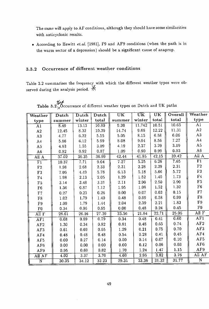
The same will apply to AF conditions, although they should have some similarities
with anticyclonic results.
• According to Hewitt et.al . [1981], F9 and AF9 conditions (when the path is in
the warm sector of a depression) should be a significant cause of anaprop.
3.3.2 Occurrence of different weather conditions
Table 3.2 summarises the frequency with which the different weather types were ob-
served during the analysis period.
Table 3.2.AOccurrence of different weather types on Dutch and UK paths
Weather Dutch Dutch Dutch UK UK I UK Overall Weather
type summer winter total summer winter total total type
Al 8.49 13.13 10.80 9.30 11.742 10.51 10.65 Al
A2 12.45 8.32 10.39 14.74 9.66 12.22 11.31 A2
A3 4.77 6.32 5.55 5.05 8.15 6.58 6.06 A3
A4 5.86 6.12 5.99 8.08 9.04 8.56 7.27 A4
A5 4.63 1.55 3.09 4.19 2.37 3.29 3.19 A5
A6 0.82 0.92 10.87 1.09 1 0.90 0.99 0.93 A6
All A 37.02 36.35 36.69 42.44 41.85 42.15 39.42 All A
Fl 10.37 7.71 9.04 7.27 5.25 6.26 7.65 Fl
F2 1.98 2.68 2.33 2.31 2.28 2.29 2.31 F2
F3 7.06 4.49 5.78 6.13 5.18 5.66 5.72 P3
F4 1.98 2.13 2.05 1.29 1.52 1.40 1.73 F4
F5 3.14 3.48 3.31 2.11 2.90 2.50 2.90 F5
P6 1.36 0.87 1.12 1.95 1.08 1.52 1.32 F6
F7 0.27 0.25 0.26 0.00 0.07 0.03 0.15 F7
F8 1.02 1.79 1.40 0.48 0.69 0.58 0.99 F8
P9 1.09 1.79 1.44 2.04 2.39 2.21 1.83 F9
P0 0.34 0.96 0.65 0.00 0.48 0.24 0.45 P0
All F 28.61 26.16 27.39 23.56 21.84 22.71 25.05 All F
AF1 0.68 0.89 0.79 0.34 0.48 0.41 0.60 AF1
AF2 1.30 0.34 0.82 0.81 0.48 0.65 0.74 AF2
AF3 0.61 0.69 0.65 1.29 0.21 0.75 0.70 AF3
AF4 0.48 0.48 0.48 0.54 0.28 0.41 0.45 AF4
AF5 0.00 0.27 0.14 0.00 0.14 0.07 0.10 AF5
AF6 0.00 0.00 0.00 0.00 0.12 0.06 0.03 AF6
AF9 0.95 0.69 0.82 1.70 1 1.24 1.47 1.15 AF9
All AF 4.02 3.37 3.70 4.69 1 2.95 3.82 3.76 All AF
N 30.35 34.12 32.23 11 29.31 1 33.36 1 31.32 31.77 11 N
49
It can be seen that, for both the Dutch and UK paths, A conditions are by far the
most common, followed by N, F and finally AF conditions. The only major difference
between the regions is that anticyclones are about 5% more frequent on UK paths
than on Dutch ones, balanced by a lower percentage of fronts. There are no obvious
seasonal differences, an important point in later discussion of the occurrence of signals
during each weather type. There are noticeable differences between, on the one hand,
fronts roughly perpendicular to signal paths (F1,3,5) and those roughly parallel to
the paths (F2,4,6). This stems from the classification scheme, which imposed stricter
conditions for a front to be 'parallel' to a path than for a front to be 'perpendicular',
so 'perpendicular' fronts would be expected to occur three times as often as 'parallel'
fronts. This is more or less what is observed.
3.3.3 Significance of signals
One goal of this project was to provide indications of which weather types gave most
interference problems. This was done using the weather data given above combined
with the signal data.
The scale of the interference problem was quantified by means of the 'significance
ratio' (SR). Using the signal data for -45dBf (the lowest observable level), the ratio
of percentage of total signals to percentage of total weather was calculated for each
weather type and season. For example, if weather type X occurred for 5% of the time
but accounted for 10% of total signals, the significance ratio would be SR(X)= 10/5,
or 2.00. If signals were produced by random processes, and not in any way dependant
on the weather conditions, the SR would be expected to be close to one. If the weather
conditions caused anaprop, the SR would be greater than one, and if the conditions
prevented or limited anaprop, the SR would be less than one. It was found that SR's
ranged from effectively zero, indicating that the weather type suppressed all anaprop,
to a maximum of nearly 5, indicating the weather type as a strong cause of anaprop.
These findings are summarised in figures 3.2 and 3.3.
On Dutch paths, the significance ratios are shown in figure 3.2. On almost all weather
types, there are clear seasonal differences, with summer giving higher SR's than winter.
Few frontal types have SR's much above one, and N has low SR's. Conversely most A
and AF types have high SR's.
On UK paths, SR's are shown in figure 3.3. Again there are clear seasonal differences,
with higher summer than winter values. Again, A and AF conditions show generally
high SR's while F and N show low values. All these results will be discussed later in
50
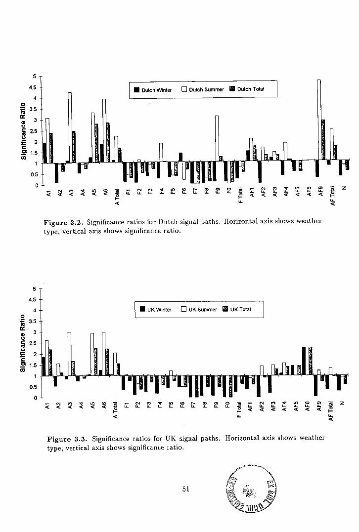
5
4.5
4 0
3.5 to cc a) U
2.5 U
2
. 1.5 U)
0.5
0 . u cc , W r- .— C'4 r U' CD O Z
< < < < < • LL. U IL. IL. LL. LL. IL. U- LI. LI. - LI. LI. LI. IL. IL. LL. LL. 16 < < < < < < <
LI. 'I.
Figure 3.2. Significance ratios for Dutch signal paths. Horizontal axis shows weather type, vertical axis shows significance ratio.
5
4.5
4 0
3.5 cc
U 2.5 cc
U
.' 1.5 Cl)
0.5
0 N M ' U) CO N. CD CD 0 N 0) U) CD CD Z
- LI. U. U. U. U. LI. U. LI. U. U. U. U. LI. LI. LI. <
U- U.
Figure 3.3. Significance ratios for UK signal paths. Horizontal axis shows weather type, vertical axis shows significance ratio.
51
this chapter.
3.3.4 Interference Data Sheets
The main method of presenting the statistical results is through a portfolio of 'inter-
ference data sheets' (IDS's). These give, for each weather type and for Dutch and UK
paths:
• A cumulative distribution showing signals at all levels for winter, summer and the
whole year, as well as a reference curve showing the total signals for all weather
types over the whole year.
• A chart showing the variation in signals over the course of a year as a percentage
of the total signals observed each month. Curves are given for three or four
different signals levels, from -45 dBf up to the free space level. This chart can
bring out the main seasonal influences on the anaprop but is also influenced by
the variation in occurrence of the weather type.
• A chart showing the behaviour of signals throughout the course of a day, again at
a number of different levels. This allows some determination of the main mecha-
nisms responsible for the anaprop, particularly during anticyclonic conditions.
• A DWR synoptic chart for a typical example of the weather type. This aids
operational use of the ID S's by giving a basis for comparison with forecast charts.
• A written summary of the results, detailing the main mechanisms likely to give
rise to the anaprop as well as giving the frequency with which the weather con-
dition occurs during the year and the significance ratios.
IDS's were produced at the request of BTL, who required statistics in a form easily used
by their engineers. The data can be used for planning purposes, giving indications of
which periods are most likely to be a risk from anaprop, as well as operationally, when
predictions of the likelihood of anaprop can be made using forecast weather charts.
The entire IDS portfolio is given as appendix A of this thesis.
3.3.5 Results for Dutch signal paths
To give an overview of the statistical results, data for all A-type conditions were merged,
as were data for all F and all AF-type conditions. With the N-type conditions, this
52
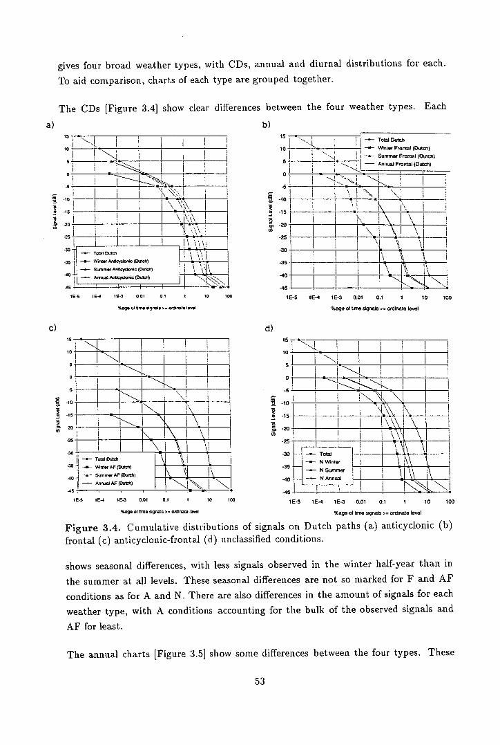
gives four broad weather types, with CDs, annual and diurnal distributions for each.
To aid comparison, charts of each type are grouped together.
The CDs [Figure 3.4] show clear differences between the four weather types. Each
a) b) 15
10
-5
it
.tt
2 .0 -25 U,
-21
-35
-35
-4
c)
-
-
-' -
I 1 Tow Dutch
WinterMticydonrc(Dslth) • II —a-- Summer An4cydsnrc(Ds4th)
AmSial As done flU)(
SE-S 56-4 554 0.01 0.1 I 10 500
%aqe SI time signals , ordinate level
15 -.-- Total Dutch --
10 —4— Winter Frontal (Dutch)
-- Summer Frontal (Dutch) 5 - Annual Frontal (Dutch)
-5 C
-10
-15
.20
-25
-30
.35
-40
-45
1E-5 16-4 16-3 0.01 0.5 1 10 100
%age of time signals x ordinate level
d)
0
[: _I
lfl\
15
to
5
0
-6
-to
-15
2 .5 -20 01
-25
-30
.35
-45
.45
15
10
5
0
.5
-10
-15
M i -20
11)
-25
-30
-35
-40
-45
a.-.--'
N\ N...
: Total L ii
—a-- N Summer
-j- NAnnual
I :Hii
SE-5 564 16-3 0.01 0.1 I 10 100 16-5 1E-4 1E-3 0.01 0.1 1 10 100
%age 01 Store signals n= ordinate level
%age of time signals >= ordinate level
Figure 3.4. Cumulative distributions of signals on Dutch paths (a) anticyclonic (b) frontal (c) anticyclonic-frontal (d) unclassified conditions.
shows seasonal differences, with less signals observed in the winter half-year than in
the summer at all levels. These seasonal differences are not so marked for F and AF
conditions as for A and N. There are also differences in the amount of signals for each
weather type, with A conditions accounting for the bulk of the observed signals and
AF for least.
The annual charts [Figure 3.5] show some differences between the four types. These
53
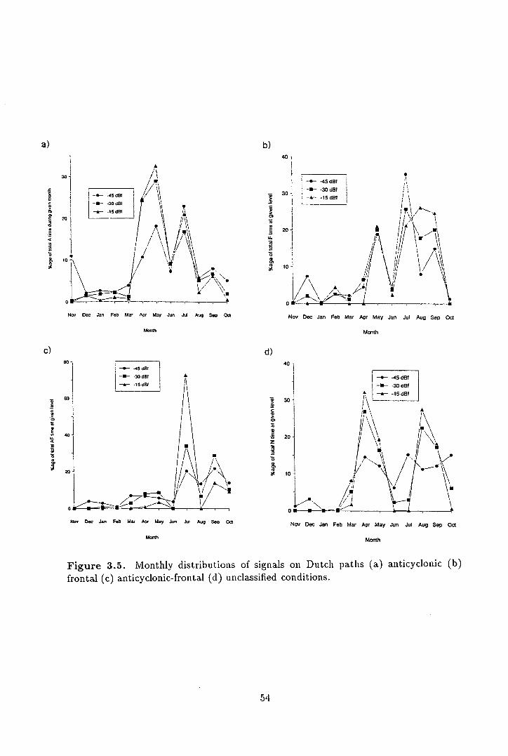
54
a)
0W
Nan Dec Jan Feb Mar Apr May Jun Jul Aug Sep Oct
Month
C)
80
- 80
S
E 40
.4
5, 20
Q • A
Non Dec Jan Feb Mar Apr May Jun ad Aug Sec Oct
Month
0S t
Nov Dec Jan Feb Mar Apr May Jun Jul Aug Sep Oct
Month
40
5 30
C P a Or
I :
0U_•_- U
Nov Dec Jan Feb Mar Apr May Jun Jul Aug Sep Oct
Month
Figure 3.5. Monthly distributions of signals on Dutch paths (a) anticyclonic (b) frontal (c) anticyclonic-frontal (d) unclassified conditions.
30
S p
20
E
to
40-I
-S- d5dBl
30j -s-- -30 dB?
C
Or
0
201 U.
0 P
lI ' 10 1
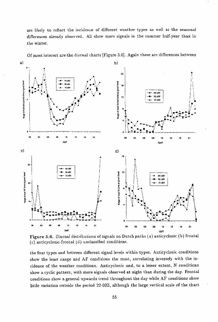
16
.0 01
12
a
8
0 01 a
4
0
00 03 06 09 12 15 18 21
GMT
are likely to reflect the incidence of different weather types as well as the seasonal
differences already observed. All show more signals in the summer half-year than in
the winter.
Of most interest are the diurnal charts [Figure 3.6]. Again there are differences between
a) b) 4
15 d131
/ ._.\ /\\ - - 30 dBf
-a- IOdBIj
4 - \ \
S ..
I 00 03 06 09 12 15 18 21
GMT
C)
30
20
S
ij 10
d) 16
12
a S 0
€8
I: 0 f -i A A l. 0 A 'A
00 03 08 09 12 15 18 21 00 03 06 09 12 15 18 21
GUT GMT
Figure 3.6. Diurnal distributions of signals on Dutch paths (a) anticyclonic (b) frontal (c) anticyclonic-frontal (d) unclassified conditions.
the four types and between different signal levels within types. Anticyclonic conditions
show the least range and AF conditions the most, correlating inversely with the in-
cidence of the weather conditions. Anticyclonic and, to a lesser extent, N conditions
show a cyclic pattern, with more signals observed at night than during the day. Frontal
conditions show a general upwards trend throughout the day while AF conditions show
little variation outside the period 22-03Z, although the large vertical scale of the chart
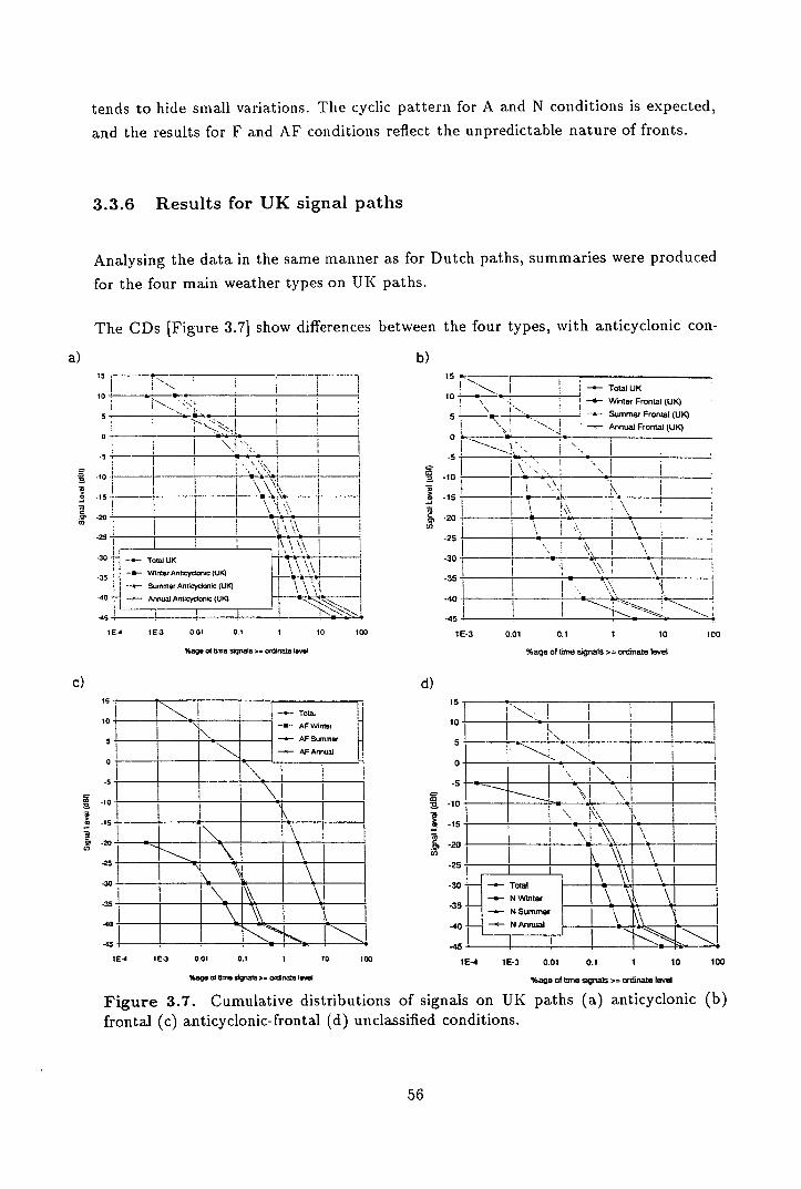
b) 15o
Total UK tO
0
-5
-10
-15
.20
-30
.35
-40
-45
- . -- Winter Frontal (UK)
Summer Fro (UK) I -. - Annual Frontal (UK)
_______
1
_
tends to hide small variations. The cyclic pattern for A and N conditions is expected,
and the results for F and AF conditions reflect the unpredictable nature of fronts.
3.3.6 Results for UK signal paths
Analysing the data in the same manner as for Dutch paths, summaries were produced
for the four main weather types on UK paths.
The CDs [Figure 3.7] show differences between the four types, with anticyclonic con-
a) 15
H 0
.5
1. 10
.15
20
.25
-31)
.35
-40
-45
154 IE-3 0.01 0.1 I 10 100
1605.01 time Signals c= ordinate level
C)
I —.-- AF Winter
AF Summer
AF Annual
1 I
1E-3 0.01 0.1 1 10 100
%age at lime signals >= ordinate level
d)
—4 N.
N ' \
11111 \J\
Li
TO
—.— NWtnter
—.— NSusnmer \ N
LI \
I \ \ \'• \ I' \ '
11111111 __
-a— Total UK
--
Winter Anyonal(UK)
-.- Summer Anlicycalnic (UK)
Amlual AntIcydoroc (UK)
I
\ \\
15
10
5
0
-5
-to
3 -15
.? -20 0,
-25
-30
.35
-40
-45
15
10
5
0
-5 C 0, •0 -10
-15
-20 in
.25
-30
-35
-40
-45
IE-4 104 0.01 0.1 1 TO 100 SE4 1E-3 0.01 0.1 1 10 tOO
1689001 time signals , OIthAOt. level %age at thvte signals s= ordinate level
Figure 3.7. Cumulative distributions of signals on UK paths (a) anticyclonic (b) frontal (c) anticyclonic-frontal (d) unclassified conditions.
56
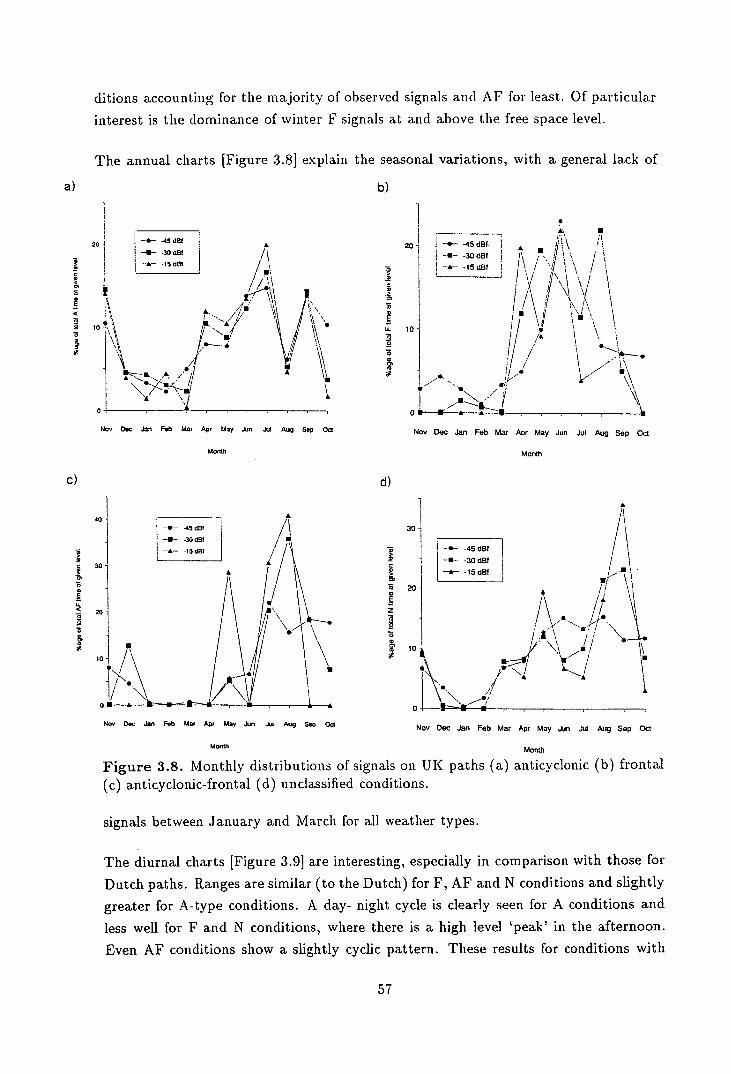
ditions accounting for the majority of observed signals and AF for least. Of particular
interest is the dominance of winter F signals at and above the free space level.
The annual charts [Figure 3.81 explain the seasonal variations, with a general lack of
a) b)
S
20
E
C 0 2 50
20 I -S-- -45d81
-U- -3OciBl
-h-- -15d8t
S
LL 10 a
0 S 0, C,
-S a
05
Nov Dec Jan Feb Mw Apr May Jan JulAug Sep Oct
Month
C)
OU —--- h - £ U
Nov Dec Jar, Feb Mar Apr May Jun JulAug Sep Oct
Month
91
40
30
a U-
20
a
Ut
SO
30
0
S
C 0
20 S S
z
0 S
g' 10
a. A. U —U -- U - U A- -L
Nov Dec Jan Feb Ma, Ay, May Jan Jul Aug Sep Oct Nov Dec Jan Feb Mar Apr May Jun Jul Aug Sep Oct
Month Month
Figure 3.8. Monthly distributions of signals on UK paths (a) anticyclonic (b) frontal (c) anticyclonic-frontal (d) unclassified conditions.
signals between January and March for all weather types.
The diurnal charts [Figure 3.91 are interesting, especially in comparison with those for
Dutch paths. Ranges are similar (to the Dutch) for F, AF and N conditions and slightly
greater for A-type conditions. A day- night cycle is clearly seen for A conditions and
less well for F and N conditions, where there is a high level 'peak' in the afternoon.
Even AF conditions show a slightly cyclic pattern. These results for conditions with
57
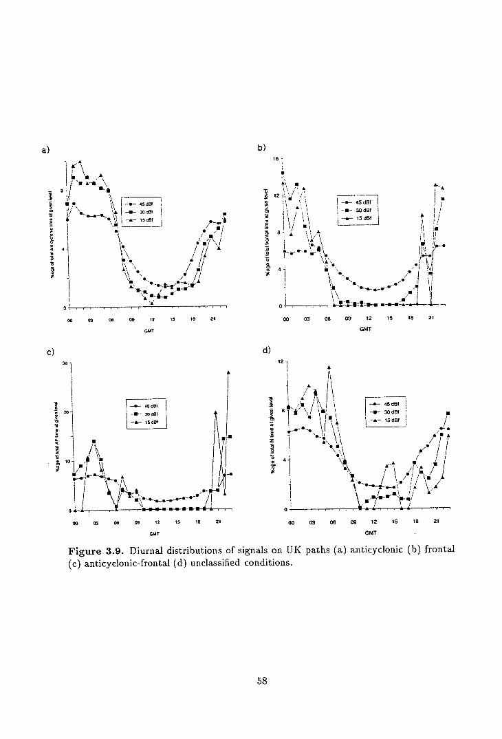
a) b) A
16-
A
sJ
• !. A
12 - A
- 45dBf
, -.-- ISM
\I_0_30dBl • J\ -u-30dBI - 1J
I.
81 \kA\ or
/75
Ar
A' 0
00 03 06 09 12 15 IS 21 00 03 06 09 12 15 18 21
GMT GMT
C) 30
20 2
8
6 10
d) 12
1 A
z
-ó
45d61
--3OdBl U
-A-- 15 d8 /
• A
/
/ \ •"! .E / i /1
I A \ A
- . •U--U-UUUA 0 .UA& . ....
00 03 06 00 12 15 18 21 00 03 06 09 12 15 18 21
GMT GMT
Figure 3.9. Diurnal distributions of signals on UK paths (a) anticyclonic (b) frontal (c) anticyclonic-frontal (d) unclassified conditions.
58
fronts are somewhat surprising.
3.4 Discussion
During the statistical analysis, some interesting results have been observed, in some
cases confirming existing expectations, and in others disagreing with them. This section
will consider the findings from the different statistical analyses.
3.4.1 Occurrence of different weather conditions
The main conclusion that can be drawn from this section is that the initial weather
classification scheme was too detailed. Of the 24 weather types considered, five (F7,
FO, AF4, AF5, AFG) occur so rarely that they could be omitted without any loss.
This could be done in any future analysis. Comparing observations for different paths
and seasons, there are few differences between winter and summer half-years, with the
notable exception of A2 conditions. AF and N conditions show few differences between
UK and Dutch paths, but A conditions are about 5% more frequent over UK paths
than over Dutch paths, balanced by a corresponding decrease in the number of fronts.
This general lack of differences between different seasons and different geographical
regions is expected from climatological studies. It is useful in that it allows the analyst
to concentrate on seasonal and geographical differences in the observed signals, without
having to take variations in the weather into account.
3.4.2 Significance of signals
Significance ratios have proved an important method of comparing different weather
types. They provide an at a glance' summary of seasonal differences and the differences
between path types.
The most obvious feature of the charts is the greater range of significances observed
on Dutch paths, where several SRs exceed 4, compared with a maximum SR of 3 for
UK paths. Different weather types have very different significances, too. A and AF
conditions generally have above-average significances on both UK and Dutch path,
while F and AF tend to have below average significance ratios. Seasonal differences
59
are also clear, with almost all weather types on both path groups showing higher SRS
in summer than in winter.
These results confirm many of the expectations of the analysis. There are clear dif -
ferences between A1/3 conditions (where advection is offshore from Europe) and A2/4
(where advection is from the UK or down the North Sea, with significant amounts of
anaprop associated with the former, and below average amounts with the latter. This
agrees with the view that high pressure to the East of the UK is a significant cause of
anaprop [Bye 1988a]. A5 and A6 conditions are also significant causes of anaprop.
Frontal conditions can be seen to be a fairly insignificant cause of anaprop on both
path types. In some cases (F7 and FO) this is due to lack of data, but for all other F
weather types there is enough data for the results to be valid. F9 conditions are, as
expected, more significant causes of anaprop than other types, but this is only clear on
Dutch signal paths. Despite this general insignificance of frontal conditions, it must be
remembered that severe anaprop can be associated with some fronts [Hewitt et.al.1981].
As expected, AF conditions are generally a significant cause of anaprop, although the
rarity of some types (AF4/5/6) makes their results suspect. AF9 conditions are seen
to be particularly significant on Dutch paths, but there are clear differences between
summer and winter half years. N conditions are not a significant cause of anaprop.
3.4.3 Interference data sheets
Produced as a reference guide for BTL engineers, the portfolio of interference data
sheets provides the statistical detail behind the summaries presented in this chapter.
There is too much information to examine in full here, and each sheet includes a
summary of the charts and the meteorological causes of the anaprop. It is hoped that
these sheets will be useful operational tools as well as a method of correlating weather
and signal data which can be used elsewhere in the world.
3.4.4 Dutch signal paths
Comparing the four main weather types (A, F, AF and N), some clear similarities are
evident. These may give clues to the mechanisms causing anaprop for different weather
types.
The cumulative distributions show similarities between F and AF conditions, as well as
60
between A and N. All four types show seasonal differences, but these are less marked
for A and N than for F and AF. These seasonal effects are likely to he caused by the
changing sea surface temperature during the year.
The same similarities are also visible on the diurnal charts, although not so clearly.
The similarities in diurnal behaviour between A and N conditions suggest the same
mechanisms at work, emphasising the message that the effects of advection, radiation
cooling and subsidence are not confined to anticyclones, but can occur during any
synoptic conditions. AF conditions show little variation throughout the day, with the
few observable peaks likely to be due to single, severe events. This lack of variation
is expected, since fronts are not constrained to any particular times of day. Frontal
conditions appear to show some diurnal variation with more signals observed as the day
progresses. This is surprising, as results similar to AF conditions are expected, with
signals distributed equally throughout the day. These results are not observed on land
paths, suggesting advection as a mechanism for the higher amounts of signals, leaving
the unresolved question of why similar patterns are not observed under AF conditions.
The monthly charts show the causes of the seasonal differences on the CDs. Each
weather type has a 'season' when the majority of signals are observed. It is difficult
to draw any conclusions from these without corresponding monthly distributions of
the weather conditions. With these, significance ratios could have been investigated
in more detail to see whether, as seems likely, much of the variation between months
reflects the incidence of that weather type. This is an area that could be addressed by
future work in this field.
Returning to the significance ratios, A and AF conditions have almost identical SRs
(around 1.7), as do F and N conditions (around 0.5). Do these SRs indicate links
between the weather types, different to the links hypothesized from the CDs and di-
urnal charts? This and other questions are in need of answers. Can AF conditions
be considered as special examples of F types, or are they more closely related to A
conditions? How do the mechanisms responsible for anaprop in anticyclones interact
with the mechanisms associated with fronts? Are the similarities in results for different
weather conditions due only to chance? Some of these questions will be examined in
the next chapter, but others will remain unanswered in this work.
3.4.5 UK signal paths
Once again, different weather types have similarities, suggesting common mechanisms
responsible for the anaprop. The links between weather types are different to those on
61
Dutch paths, again raising questions to be answered.
The CDs show similarities in the results for F, AF and N conditions, with the vast
majority of recorded signals in the summer half year. Anticyclonic conditions still
show a difference between the seasons, but it is less marked than for the other types.
Above the free space level, both F and A conditions show more signals in winter than in
summer, a feature not observed on Dutch paths. Because of the small time percentages
involved (less than 0.01% of the time), these are likely to be the product of a very small
number of events.
Diurnal charts show similar patterns, with more signals during darkness than daylight.
The variation in about the same on each chart once differences in scale are taken into
account. A closer examination shows the diurnal pattern to be less pronounced during
AF conditions than during the others, suggesting a mechanism independent of time as
the cause. This is similar to the observations for Dutch paths, but F conditions show
a very different pattern.
As on Dutch paths, it is difficult to draw any conclusions from the monthly charts
without more weather data. It is clear that signals are more common in summer than
in winter, but it would be necessary to produce monthly significance ratios to see how
important an effect this is.
The SRs for F and N conditions are very close, as observed on Dutch paths, but A and
AF conditions have very different SRs. Is this indicative of the same causes for anaprop
under F and N conditions? What causes the differences between UK and Dutch results
- are they all due to the effects of advection, as suggested by the BTL model, or are
they purely chance. Again some of these questions will be examined later in this work,
while others will remain for the radio-meteorologists of the future.
3.4.6 Conclusions
This analysis has confirmed the importance of anticyclones as a cause of anaprop as
well as showing fronts to be a relatively insignificant cause. This does not mean that
fronts can be ignored - they are still a problem when individual events cause severe
anaprop, but they are relatively trivial for the purposes of network planning. The
interactions of fronts with anticyclones are more important than fronts alone, but since
they occur rarely, they also have little statistical importance.
The techniques used to analyse and correlate signal and weather data are based on the
62

existing tools used by radio scientists. It is hoped that further studies of the effects of
weather on signals will be undertaken, so better models of the links between weather,
anaprop mechanisms and signals can he developed.
63

Chapter 4
Conceptual models of fronts and
anaprop
This chapter examines fronts and depressions through a number of conceptual models,
similar to the BTL anticyclone model, which provide a physical explanation of the
processes occurring in typical depressions of different types. The models are based on
current meteorological knowledge, adapted to radio-meteorology. It must he stressed
that the models are qualitative, not quantitative. This is clue to the great variety of
fronts, which can change dramatically in both the space and time scales, as well as the
relatively small amount of hard data available to quantify the models. These models
were developed in parallel with the case studies presented in the next two chapters,
and were modified continually during the analysis process.
The chapter begins with a survey of existing work on fronts and depressions, looking
in slightly more detail than usual at the conceptual models that will be used as a basis
for the remainder of this chapter. This is followed by a discussion of the adaptations
needed to use the meteorological models for radio-meteorology and then by a series of
studies of different types of fronts—ana-type, kata-type (with and without upper cold
fronts) and occlusions. For each type, there is an examination of conditions leading to
anaprop, and (qualitative) predictions of the likelihood of anaprop being observed. To
close the chapter, there is a brief look at warm sector subsidence and the relationship
between fronts and anticyclones.
64
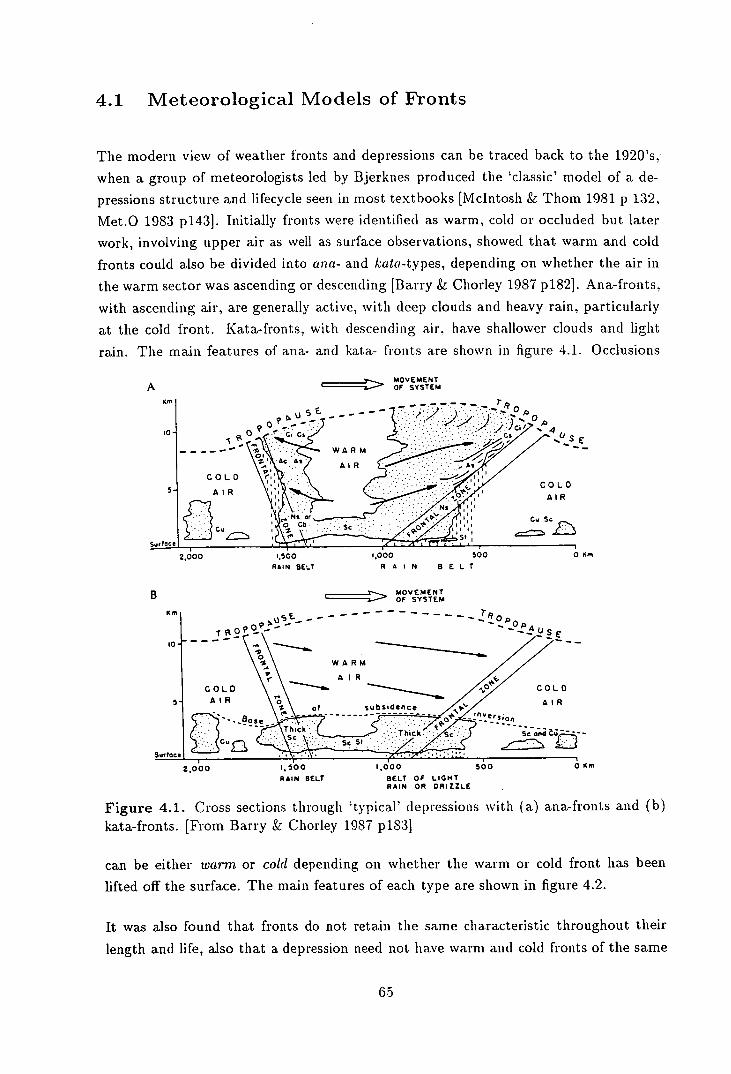
4.1 Meteorological Models of Fronts
The modern view of weather fronts and depressions can be traced back to the 1920's,
when a group of meteorologists led by Bjerknes produced the 'classic' model of a de-
pressions structure and lifecycle seen in most textbooks [McIntosh & Thom 1981 p 132,
Met.O 1983 p143]. Initially fronts were identified as warm, cold or occluded but later
work, involving upper air as well as surface observations, showed that warm and cold
fronts could also be divided into ana- and kata-types, depending on whether the air in
the warm sector was ascending or descending [Barry & Chorley 1987 p1821. Ana-fronts,
with ascending air, are generally active, with deep clouds and heavy rain, particularly
at the cold front. Kata-fronts, with descending air, have shallower clouds and light
rain. The main features of ana- and kata- fronts are shown in figure 4.1. Occlusions
c- MOVEMENT OF SYSTEM
WARM
ISIS
cu Sc
cu 0 cb SC
st
2,000 1.500 1,000 500
RAIN BELT RAIN BELT
B MOVEMENT OF SYSTEM
Km
WARM
COLD COLO
5- AIR AIR subsiden
Thick* SO
2,000 1,500 1,000 500
RAIN BELT BELT OF LIGHT RAIN OR DRIZZLE
Figure 4.1. Cross sections through 'typical' depressions with (a) ana-fronts and (b) kata-fronts. [From Barry & Chorley 1987 p 183]
can be either warm or cold depending on whether the warm or cold front has been
lifted off the surface. The main features of each type are shown in figure 4.2.
It was also found that fronts do not retain the same characteristic throughout their
length and life, also that a depression need not have warm and cold fronts of the same
65
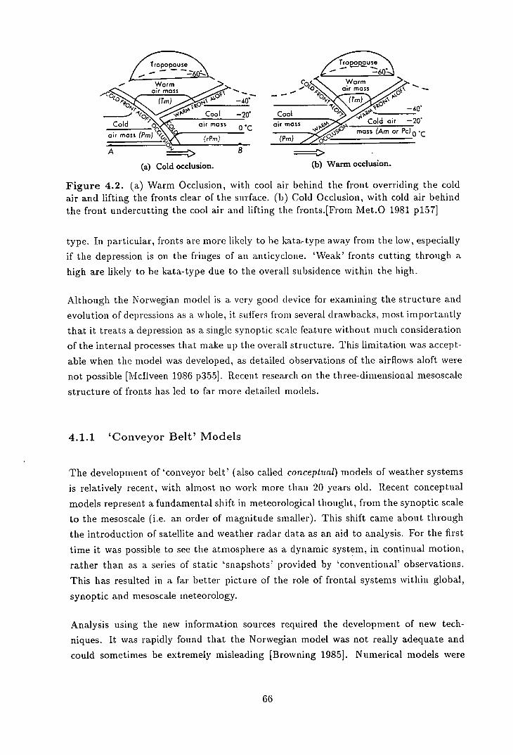
Tropopouse
Worm air cT ass
Cool —20*
Cold air moss air moss
A
(a) Cold occlusion.
lroeo`pa-se
Co <<N Worm air moss
-•::Cold air air moss ________________
mass (Am or Pc) ()
(b) Warm occlusion.
Figure 4.2. (a) Warm Occlusion, with cool air behind the front overriding the cold air and lifting the fronts clear of the surface. (h) Cold Occlusion, with cold air behind the front undercutting the cool air and lifting the fronts.[From Met.O 1981 p157]
type. In particular, fronts are more likely to be kata-type away from the low, especially
if the depression is on the fringes of an anticyclone. "Weak' fronts cutting through a
high are likely to he kata-type due to the overall subsidence within the high.
Although the Norwegian model is a very good device for examining the structure and
evolution of depressions as a. whole, it suffers from several drawbacks, most importantly
that it treats a depression as a single synoptic scale feature without much consideration
of the internal processes that make up the overall structure. This limitation was accept-
able when the model was developed, as detailed observations of the airflows aloft were
not possible [Mdllveen 1986 p3551. Recent research on the three-dimensional mesoscale
structure of fronts has led to fax more detailed models.
4.1.1 'Conveyor Belt' Models
The development of 'conveyor belt' (also called conceptual) models of weather systems
is relatively recent, with almost no work more than 20 years old. Recent conceptual
models represent a fundamental shift in meteorological thought, from the synoptic scale
to the mesoscale (i.e. an order of magnitude smaller). This shift came about through
the introduction of satellite and weather radar data as an aid to analysis. For the first
time it was possible to see the atmosphere as a dynamic system, in continual motion,
rather than as a series of static 'snapshots' provided by 'conventional' observations.
This has resulted in a far better picture of the role of frontal systems within global,
synoptic and mesoscale meteorology.
Analysis using the new information sources required the development of new tech-
niques. It was rapidly found that the Norwegian model was not really adequate and
could sometimes be extremely misleading [Browning 1985]. Numerical models were
66
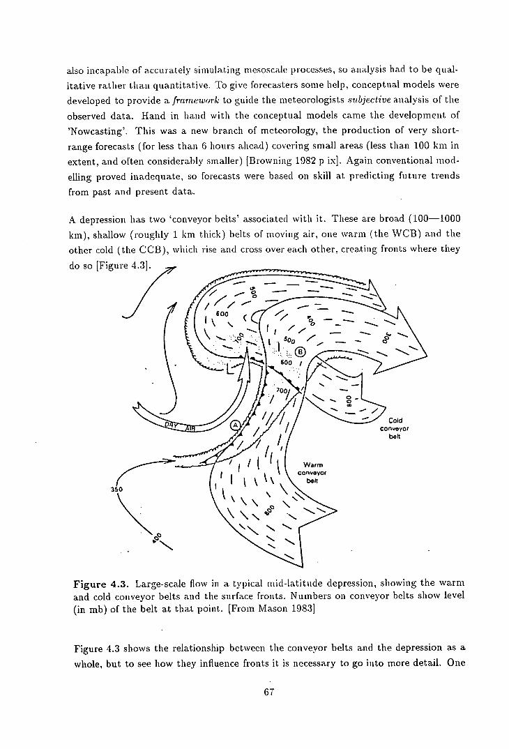
also incapable of accurately simulating mesoscale processes, so analysis had to be qual-
itative rather than quantitative. To give forecasters some help, conceptual models were
developed to provide a framework to guide the meteorologists subjective analysis of the
observed data. Hand in hand with the conceptual models came the development of
'Nowcasting'. This was a new branch of meteorology, the production of very short-
range forecasts (for less than 6 hours ahead) covering small areas (less than 100 km in
extent, and often considerably smaller) [Browning 1982 p ix]. Again conventional mod-
elling proved inadequate, so forecasts were based on skill at predicting future trends
from past and present data.
A depression has two 'conveyor belts' associated with it. These are broad (100-1000
km), shallow (roughly 1 km thick) belts of moving air, one warm (the WCB) and the
other cold (the CCB), which rise and cross over each other, creating fronts where they
do so [Figure 4.3]. .
Figure 4.3. Large-scale flow in a typical mid-latitude depression, showing the warm and cold conveyor belts and the surface fronts. Numbers on conveyor belts show level (in mb) of the belt at that point. [From Mason 19831
Figure 4.3 shows the relationship between the conveyor belts and the depression as a
whole, but to see how they influence fronts it is necessary to go into more detail. One
67
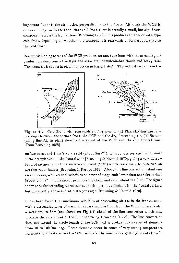
important factor is the air motion perpendicular to the fronts. Although the WCB is
shown running parallel to the surface cold front, there is actually a small, but significant
component across the frontal zone [Browning 1985]. This produces an ana- or kata-type
cold front, depending on whether this component is rearwards or forwards relative to
the cold front.
Rearwards sloping ascent of the WCB produces an ana-type front with the ascending air
producing a deep convective layer and associated cumulonimbus clouds and heavy rain.
The structure is shown in plan and section in Fig 4.4 [ibid.]. The vertical ascent from the
(0)
D.sc.nthng ___ dry a.r —In
10- lOwd.'
\
Warm
/ conw.vot bell
d
(b)
6 L. -
,
LU
a I A Sorloc. •
cold hani
Figure 4.4. Cold Front with rearwards sloping ascent. (a) Plan showing the rela-tionships between the surface front, the CCB and the dry, descending air. (b) Section (along line AB in plan) showing the ascent of the WCB and tile cold frontal zone. [From Browning 1985]
surface to around 2 km is very rapid (about 5ms'). This zone is responsible for most
of the precipitation in the frontal zone [Browning & Harrold 1970], giving a very narrow
band of intense rain at the surface cold front (SCF) which can clearly be observed on
weather radar images [Browning & Pardoe 1973]. Above this line convection, slantwise
ascent occurs, with vertical velocities an order of magnitude lower than near the surface
(about 0.477i.$). This ascent produces the cloud and rain behind the SCF. The figure
shows that the ascending warm conveyor belt does not coincide with the frontal surface,
but lies slightly above and at a steeper angle [Browning & Harrold 1970].
It has been found that maximum velocities of descending air are in the frontal zone,
with a descending layer of warm air separating the front from the WCB. There is also
a weak return flow (not shown on Fig 4.4) ahead of the line convection which may
produce the rain ahead of the SCF shown by Browning [1985]. The line convection
does not extend the whole length of the SCF, but is broken into a series of elements
from 10 to 100 km long. These elements occur in zones of very strong temperature
horizontal gradients across the SCF, separated by much more gentle gradients [ibid.].
68
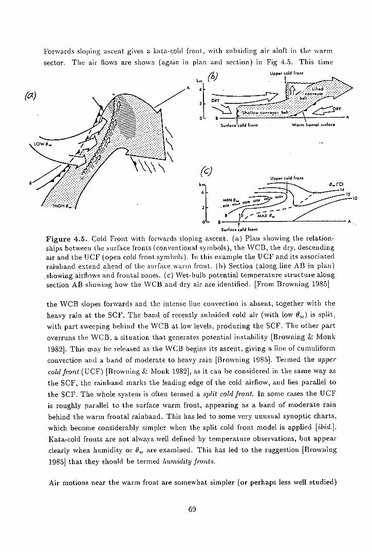
Forwards sloping ascent gives a. kata.-cold front., with subsiding air aloft in the warm
sector. The air flows are shown (again in plan and section) in Fig 4.5. This time
(c) Upper cold front
km
BL' T
6 14
mlN 8_ 10
Surface cold Front
Figure 4.5. Cold Front with forwards sloping ascent. (a) Plan showing the relation-ships between the surface fronts (conventional symbols), the WCB, the dry, descending air and the UCF (open cold front symbols). In this example the UCF and its associated rainband extend ahead of the surface warm front. (b) Section (along line AB in plan) showing airflows and frontal zones. (c) Wet-bulb potential temperature structure along section AB showing how the WCB and dry air are identified. [From Browning 1985]
the WCB slopes forwards and the intense line convection is absent, together with the
heavy rain at the SCF. The band of recently subsided cold air (with low 9,,) is split,
with part sweeping behind the WCB at low levels, producing the SCF. The other part
overruns the WCB, a situation that generates potential instability [Browning & Monk
1982]. This may be released as the WCB begins its ascent, giving a line of curnuliform
convection and a band of moderate to heavy rain [Browning 19851. Termed the upper
cold front (UCF) [Browning & Monk 1982], as it can be considered in the same way as
the SCF, the rainband marks the leading edge of the cold airflow, and lies parallel to
the SCF. The whole system is often termed a split cold front. In some cases the UCF
is roughly parallel to the surface warm front, appearing as a band of moderate rain
behind the warm frontal rainband. This has led to some very unusual synoptic charts,
which become considerably simpler when the split cold front model is applied [ibid.].
Kata-cold fronts are not always well defined by temperature observations, but appear
clearly when humidity or 0,, are examined. This has led to the suggestion [Browning
1985] that they should be termed humidity fronts.
Air motions near the warm front are somewhat simpler (or perhaps less well studied)
b Upper cold Front
A
k
DRY
Surloc.'cold front Worm lronial surface
69
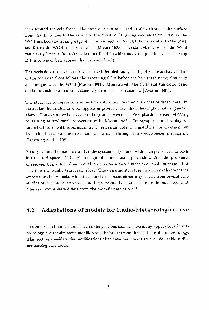
than around the COl(l front. The band of cloud and precipitation ahead of the surface
front (SWF) is due to the ascent of the moist WCB giving condensation. Just as the
WCB marked the trailing edge of the warm sector, the CCB flows parallel to the SWF
and forces the WCB to ascend over it [Mason 1983]. The slantwise ascent of the WCB
can clearly be seen from the isobars on Fig 4.3 (which mark the position where the top
of the conveyor belt crosses that pressure level).
The occlusion also seems to have escaped detailed analysis. Fig 4.3 shows that the line
of the occluded front follows the ascending CCB before the belt turns anti cycloni cally
and merges with the WCB [Mason 1983]. Alternatively the CCB and the cloud band
of the occlusion can curve cyclonically around the surface low [Weston 19871.
The structure of depressions is considerably more complex than that outlined here. In
particular the rainbands often appear in groups rather than the single bands suggested
above. Convection cells also occur in groups, Mesoscale Precipitation Areas (MPA's),
containing several small convection cells [Mason 1983]. Topography can also play an
important role, with orographic uplift releasing potential instability or creating low
level cloud that can increases surface rainfall through the seeder-feeder mechanism
[Browning & Hill 1981].
Finally it must be made clear that the system is dynamic, with changes occurring both
in time and space. Although conceptual models attempt to show this, the problems
of representing a four dimensional process on a, two dimensional medium mean that
much detail, usually temporal, is lost. The dynamic structure also means that weather
systems are individuals, while the models represent either a synthesis from several case
studies or a detailed analysis of a. single event. It should therefore be expected that
"the real atmosphere differs from the model's predictions"!
4.2 Adaptations of models for Radio-Meteorological use
The conceptual models described in the previous section have many applications in me-
teorology but require some modifications before they can he used in radio-meteorology.
This section considers the modifications that have been made to provide usable radio-
meteorological models.
EEO

4.2.1 Objectives
The models developed for this work are similar in idea to the BTL conceptual model
of an anticyclone [Bye 1988a]. They show the physical processes at work and indicate
the resulting potential for anaprop. A number of different models were developed, to
cover as broad a range of frontal characteristics as possible. They are:
• A depression with ana-fronts [Section 4.31.
• A depression with kata-fronts and no Upper Cold Front [Section 4.4].
• A depression with kata-fronts and an Upper Cold Front [Section 4.51.
• Warm and cold occlusions [Section 4.61.
Estimates of the probability of anaprop axe given for each type of depression under two
sets of conditions:
• Over a warm surface (land during the day or a warm sea).
• Over a cold surface (land during the night or a cool sea).
It is felt that these options cover almost all types of fronts in sufficient detail to be usable
operationally. It should be stressed that the models are based on current meteorological
thinking, and no new concepts are involved. What is new, however, is their application
to radio-meteorology.
4.2.2 Anaprop associated with Fronts
Many features of the radio-meteorological models are familiar from the standard con-
ceptual models, in particular the conveyor belts and the frontal zones. To adapt the
models to radio-meteorology, super-refractive layers have been added where appropri-
ate.
Ahead of the warm front' and behind the cold front there are super-refractive lay-
ers (SRLs), which the author has termed leading and trailing edge SRLs respectively
[Fig 4.6], that slope gently upwards away from the fronts. The slope is due to the
1 Front refers to the surface front, while frontal zone refers to the front aloft.
71
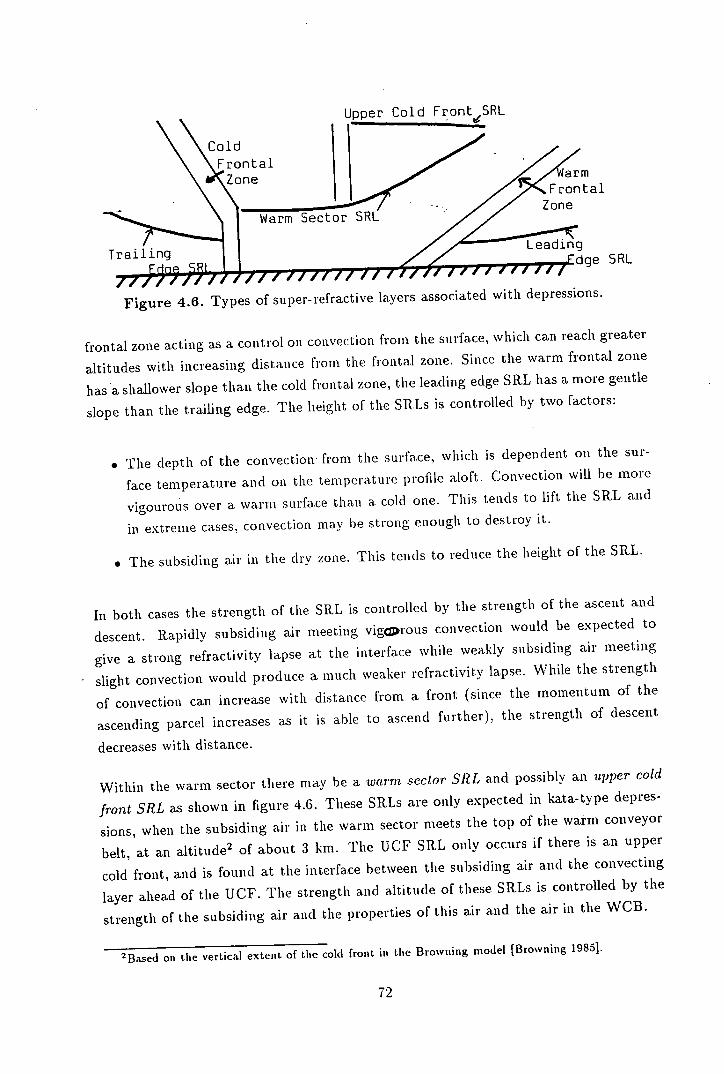
Upper Cold Front SRL I -
,' Warm Frontal Zone
Leading - -Edge SRL
Figure 4.6. Types of super-refractive layers associated with depressions.
frontal zone acting as a control on convection from the surface, which can reach greater
altitudes with increasing distance from the frontal zone. Since the warm frontal zone
has a shallower slope than the cold frontal zone, the leading edge SRL has a more gentle
slope than the trailing edge. The height of the SilLs is controlled by two factors:
• The depth of the convection from the surface, which is dependent on the sur-
face temperature and on the temperature profile aloft. Convection will be more
vigourous over a warm surface than a. cold one. This tends to lift the SRL and
in extreme cases, convection may be strong enough to destroy it.
The subsiding air in the dry zone. This tends to reduce the height of the SRL.
In both cases the strength of the SRL is controlled by the strength of the ascent and
descent. Rapidly subsiding air meeting vigorous convection would be expected to
give a strong refractivity lapse at the interface while weakly subsiding air meeting
slight convection would produce a much weaker refractivity lapse. While the strength
of convection can increase with distance from a front (since the momentum of the
ascending parcel increases as it is able to ascend further), the strength of descent
decreases with distance.
Within the warm sector there may be a warm sector SRL and possibly an upper cold
front SRL as shown in figure 4.6. These SRLs are only expected in kata-type depres-
sions, when the subsiding air in the warm sector meets the top of the warm conveyor
belt, at an altitude of about 3 km. The UCF SRL only occurs if there is an upper
cold front, and is found at the interface between the subsiding air and the convecting
layer ahead of the UCF. The strength and altitude of these SRLs is controlled by the
strength of the subsiding air and the properties of this air and the air in the WCB.
2Based on the vertical extent. of the cold front. in the Browning model [Browning 1985.
72
It might be expected that advection ducts will form when the WCB flows over the sea.
In the author's opinion these are unlikely since (for depressions affecting North West
Europe) the air in the WCB typically is of tropical maritime origin and is therefore
moist, compared with the classic advection duct formed when warm dry air flows over
a cooler sea.
4.2.3 Effects of surface temperature
As mentioned earlier, the conceptual models cover two situations - when fronts are
over warm and cool surfaces.
When fronts are over a warm surface (e.g. land during the day or when air flows over
a warmer sea) there is convection beneath the leading and trailing edge SRLs. This
would tend to lift and eventually disperse the SRLs, thus reducing the probability of
anaprop. Over a cool surface (e.g. the land during the night or when air flows over a
cooler sea) there is little convection, thus the leading and trailing edge SRLs can sink
to lower levels, just as the subsidence inversion in an anticyclone descends during the
night [Bye 1988a], so increasing the probability of anaprop on surface paths. This is
shown in figure 4.7.
Cold
Key
5RL (Warm surface) ' SRL (Cool surface)
ZoneWarm
Zone Frontal
Figure 4.7. Effects of surface temperature on the leading and trailing edge SR.Ls. The warm surface case is shown as a solid line while the cool surface case is shown as
a broken line.
It is not clear at what level the leading and trailing edge SRLs will be found. Browning
[1985] shows air subsiding in the dry zones to around 1 km, so it will be assumed here
that the leading and trailing edge SltLs will be found between 1 and 2 km (depending
on the strength and depth of the convection), near their fronts, and at higher levels
further from the fronts. Examination of data from the FRONTS'87 project (chapter 5)
will provide some verification of these values.
73
4.2.4 A word of warning!
The conceptual models presented here represent typical depressions, but it cannot be
stressed enough that 'real' weather rarely matches textbook examples. In particular
the scales of depressions vary considerably. The models presented here are of typical
mature depressions, but should be easy to adapt to other cases.
Since the models are qualitative, they give no indications of the strength of the SltLs,
and only a vague idea of their altitude and extent. This is not a drawback since the
models are intended to be a framework for the interpretation of observations which
may provide the missing details.
It is assumed throughout the following material that the whole of a depression has
either ana- or ka.ta.-type fronts. This is purely to make it easier to describe the SRLs
and anaprop associated with given types of fronts and is not intended to imply that in
'real' depressions warm and cold fronts are always of the same type. In fact real fronts
can change character along their length, and with time, but providing the characteristics
of a front at a particular point are known, the models can he applied to show what
SRLs and anaprop are expected.
4.3 Depressions with Ana-fronts
In a depression with ana-fronts there is general ascent in the warm sector, so any
anaprop is associated with the leading and trailing edge SRLs alone.
4.3.1 Structure
A plan of a typical depression with ana-fronts is shown in figure 4.8. The line AB
marks the section shown in figure 4.9. The main features to note are the trailing edge
SRL immediately behind the surface cold front and the leading edge Sill starting an
estimated 50-100 km ahead of the surface warm front. These are formed at the interface
between the dry air descending just below the frontal zones and the convection from
the surface (over a warm surface) or the turbulent boundary layer (over a cold surface).
The leading edge SRL is predicted to have a width of 100-200 km, thus extending up
to 300 km ahead of the surface front, while the trailing edge SRL is predicted to extend
only some 50-100 km, due to the greater slope of the cold front, which allows the depth
of convection to increase more rapidly with distance from the cold front than from the
74
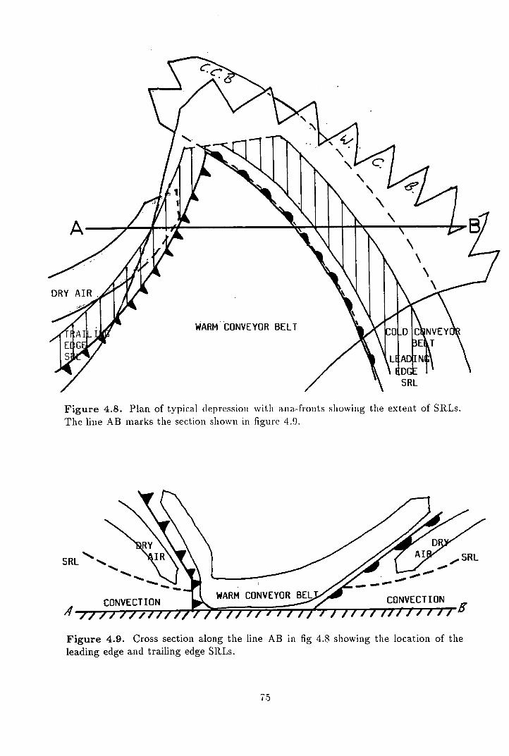
Figure 4.8. Plan of typical depression with ana-fronts showing the extent of SRLs. The line AB marks the section shown in figure 4.9.
7~ IRY
SRL'
00* Z.00 00
SRL
CONVECTION
}5WRM CONVEYOR B L CONVECTION Iff
Figure 4.9. Cross section along the line AB in fig 4.8 showing the location of the leading edge and trailing edge SRLs.
75
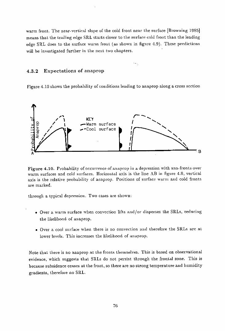
warm front. The near-vertical slope of the cold front near the surface [Browning 19851
means that the trailing edge SRL starts closer to the surface cold front than the leading
edge SRL does to the surface warm front (as shown in figure 4.9). These predictions
will be investigated further in the next two chapters.
4.3.2 Expectations of anaprop
Figure 4.10 shows the probability of conditions leading to anaprop along a cross section
KEY / ..—Warm surface I
.-Coo]. surface
A
Figure 4.10. Probability of occurrence of anaprop in a depression with ana-fronts over warm surfaces and cold surfaces. Horizontal axis is the line AB in figure 4.9, vertical axis is the relative probability of ariaprop. Positions of surface warm and cold fronts are marked.
through a typical depression. Two cases are shown:
. Over a warm surface when convection lifts and/or disperses the SRLs, reducing
the likelihood of anaprop.
. Over a cool surface when there is no convection and therefore the SRLs are at
lower levels. This increases the likelihood of anaprop.
Note that there is no anaprop at the fronts themselves. This is based on observational
evidence, which suggests that SRLs do not persist through the frontal zone. This is
because subsidence ceases at the front, so there are no strong temperature and humidity
gradients, therefore no SRL.
76
4.3.3 Discussion
In a depression with ana-fronts, SRLs are expected in a relatively narrow fringe, some
100-200 km in width, ahead of and behind the surface fronts. The anaprop "footprint"
reflects this configuration, with the long distance propagation possible when signals are
transmitted parallel to a front, and a decreasing range - as the angle between the path
and the front increases. The absence of a warm sector SRL means that a depression
has two periods of anaprop, separated by the passage of the warm sector. Depending
on the distance of the path from the low pressure centre and on the movement and
spacing of the fronts, this gap may last as long as 24 hours, or be almost non-existent.
4.4 Kata-type depressions without an Upper Cold Front
In this type of depression there is general subsidence in the warm sector, and no con-
vection above the warm conveyor belt. Anaprop is therefore associated with leading
and trailing edge SRLs together with an extended warm-sector SRL.
4.4.1 Structure
A plan of a typical depression of this type is given in figure 4.11. The line AB marks the
section shown in figure 4.12. The leading and trailing edge SRLs are the same as those
associated with ana-fronts, although it could be argued that the general subsidence
throughout the depression enhances the subsidence in the dry zones and thus lowers
and strengthens the leading and trailing edge SR.Ls. The cold front is severely limited
in vertical extent, and there is a warm sector SRL at the interface between the top of
the WCB and the base of the subsiding air. This SRL rises parallel to the WCB and
may extend above the leading edge SRL, as shown in figure 4.12.
4.4.2 Expectations of anaprop
In figure 4.13 we see the expected probability of anaprop along the cross section AB.
Once again, warm surface and cold surface cases are shown, and the leading and trailing
edge SRLs show the same expectation of anaprop as those for ana-fronts. The warm
sector SRL slopes upwards from the left to right so the probability of anaprop falls
slowly as this occurs. Since this SRL is at a higher level than the leading and trailing
7 7
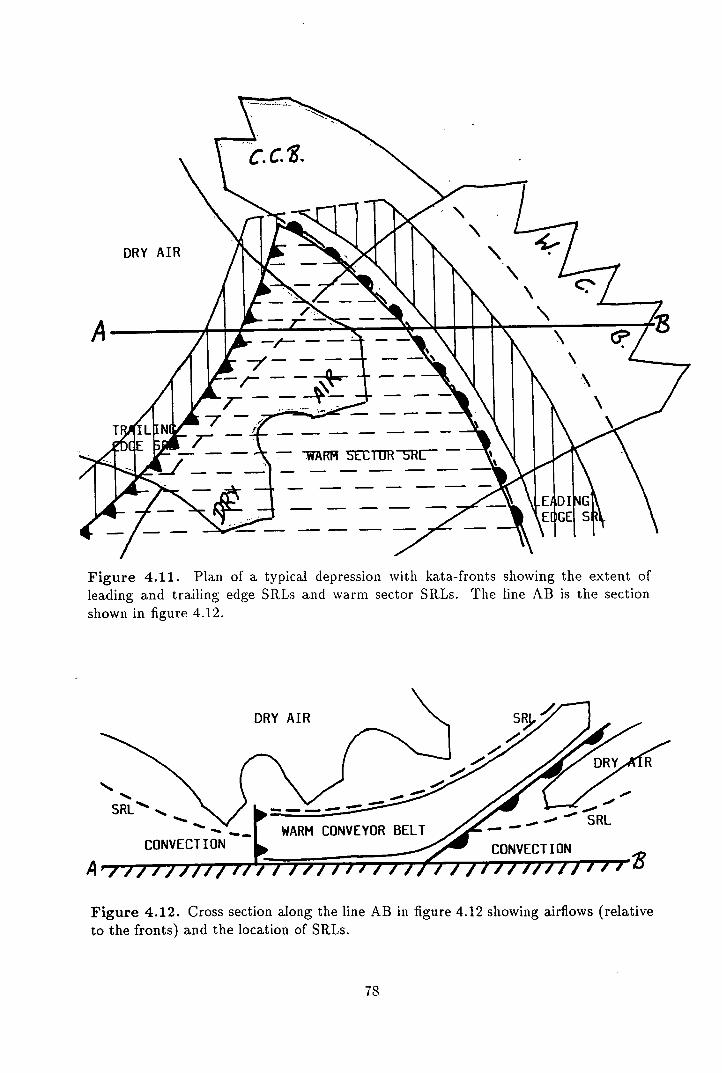
Figure 4.11. Plan of a typical depression with kata-fronts showing the extent of leading and trailing edge SRLs and warm sector SR.Ls. The line AB is the section shown in figure 4.12.
SR
IT SRL
CONVECTION
A
Figure 4.12. Cross section along the line AB in figure 4.12 showing airflows (relative to the fronts) and the location of SRLs.
78
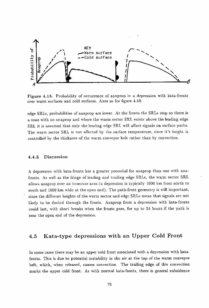
0 F'
I' >' I CL
CL
CO C
KEY ,.-Warm surface --Cold surface
1
Figure 4.13. Probability of occurrence of anaprop in a depression with kata-fronts over warm surfaces and cold surfaces. Axes as for figure 4.10.
edge SRLs, probabilities of anaprop are lower. At the fronts the SRLs stop so there is
a zone with no anaprop and where the warm sector SRL exists above the leading edge
SRL it is assumed that only the leading edge SR.L will affect signals on surface paths.
The warm sector SRL is not' affected by the surface temperature, since it's height is
controlled by the thickness of the warm conveyor belt rather than by convection.
4.4.3 Discussion
A depression with kata-fronts has a greater potential for anaprop than one with ana-
fronts. As well as the fringe of leading and trailing edge SRLs, the warm sector SRL
allows anaprop over an immense area (a depression is typically 1000 km from north to
south and 1000 km wide at the OCfl end). The path-front geometry is still important,
since the different heights of the warm sector and edge SRLs mean that signals are not
likely to be ducted through the fronts. Anaprop from a depression with kata-fronts
could last, with short breaks when the fronts pass, for up to 24 hours if the path is
near the open end of the depression.
4.5 Kata-type depressions with an Upper Cold Front
In some cases there may be an upper cold front associated with a depression with kata-
fronts. This is due to potential instability in the air at the top of the warm conveyor
belt, which, when released, causes convection. The trailing edge of this convection
marks the upper cold front. As with normal kata-fronts, there is general subsidence
79
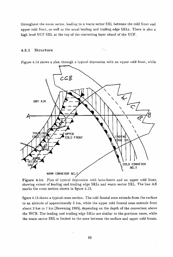
throughout the warm sector, leading to a warm sector SRL between the cold front and
upper cold front, as well as the usual leading and trailing edge SRLs. There is also a
high level UCF SRL at the top of the convecting layer ahead of the UCF.
4.5.1 Structure
Figure 4.14 shows a plan through a typical depression with an tipper cold front, while
Figure 4.14. Plan of typical depression with kata-fronts and an upper cold front, showing extent of leading and trailing edge SRLs and warm sector SRL. The line AB marks the cross section shown in figure 4.15.
figure 4.15 shows a typical cross section. The cold frontal zone extends from the surface
to an altitude of approximately 3 km, while the upper cold frontal zone extends from
about 3 km to 7 km [Browning 19851, depending on the depth of the convection above
the WCB. The leading and trailing edge SRLs are similar to the previous cases, while
the warm sector SRL is limited to the zone between the surface and upper cold fronts.
80
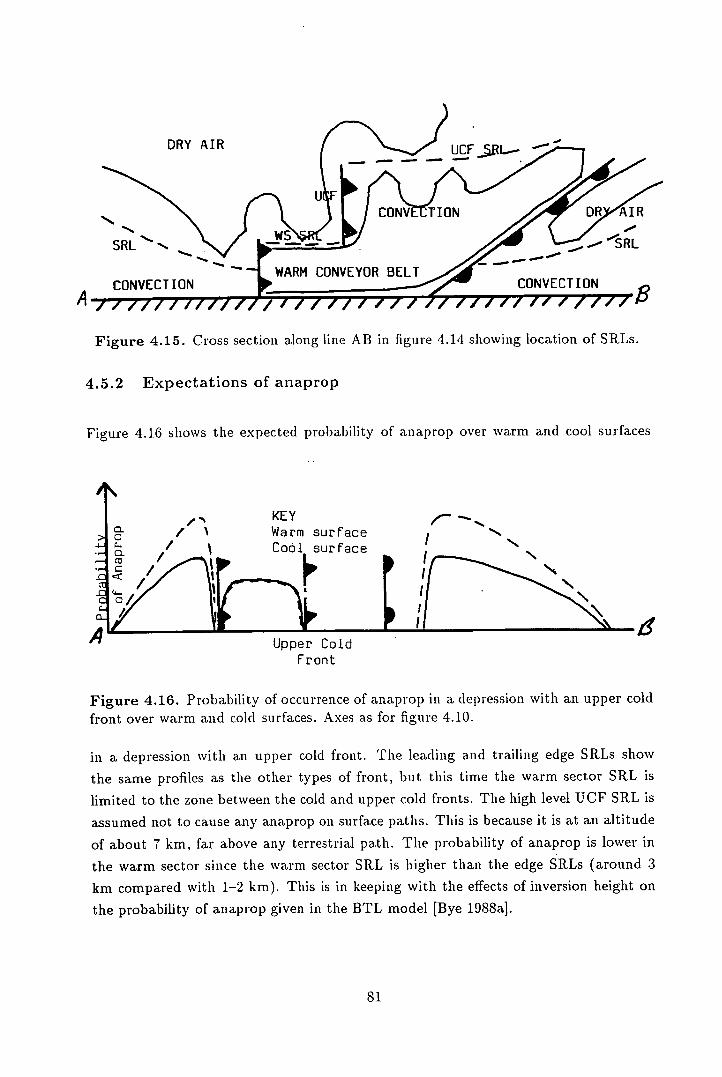
DRY AIR
SRL -
CONVECTION A ,,,,, r7
- -< UCFL2
A CONVECTION DR I
WARM CONVEYOR CONVECTION
1, flfJ FJI1JJ Z
Figure 4.15. Cross section along line AB in figure 4.14 showing location of SRLs.
4.5.2 Expectations of anaprop
Figure 4.16 shows the expected probability of anaprop over warm and cool surfaces
KEY -S I
I'
Warm surface Cool surface
/flT \ A Upper Cold
ri
Front
Figure 4.16. Probability of occurrence of anaprop in a depression with an upper cold front over warm and cold surfaces. Axes as for figure 4.10.
in a depression with an upper cold front. The leading and trailing edge SRLs show
the same profiles as the other types of front, but this time the warm sector SRL is
limited to the zone between the cold and upper cold fronts. The high level UCF SRL is
assumed not to cause any anaprop on surface paths. This is because it is at an altitude
of about 7 km, far above any terrestrial path. The probability of anaprop is lower in
the warm sector since the warm sector SRL is higher than the edge SRLs (around 3
km compared with 1-2 km). This is in keeping with the effects of inversion height on
the probability of anaprop given in the BTL model [Bye 1988a].
E1!

4.5.3 Discussion
Since low level (less than 3-4 km altitude) SRLs extend over a smaller area in a kata-
type depression with an UCF than in one without, anaprop is a less serious problem
than before, although more so than in a depression with ana-fronts. Three separate
periods of anaprop are expected, associated with the leading, warm sector and trailing
edge SRLs respectively. If the path is near the open end of the depression, there may be
a considerable gap between the leading edge and warm sector SRLs while if the path is
near the low pressure centre there may be only a short break as the warm front passes.
Since all three SRLs are relatively narrow, the path/front geometry is important, with
signals transmitted at small angles to the fronts propagating over far longer distances
than those transmitted nearly perpendicular to the front.
4.6 Occluded depressions
As a depression becomes occluded, the warm sector is squeezed upwards, leaving a
weak occluded front extending down to the surface. The formation of a warm or cold
occlusion depends on the relative temperatures of the air masses ahead of and behind
the occlusion. If the air behind the occlusion is warmer, it will override the air ahead,
lifting the cold front. If the air ahead is warmer, the cold air behind will undercut it,
resulting in the warm front being lifted [Figure 4.2]. As a consequence of this, either
the leading or trailing edge SRL is lifted considerably, while the other SRL is lifted
only slightly (if at all), resulting in anaprop on one side of the front only.
4.6.1 Warm occlusions
In a warm occlusion, air behind the depression is warmer than the air ahead of it.
When the warm sector is squeezed out, the trailing airmass rises up the occluded front,
which is effectively a weak warm front [Figure 4.171. The trailing edge SRL has been
lifted by the ascending air and is too high to cause anaprop on surface paths. The
leading edge SRL has also been lifted slightly, due to the ascent of the cold conveyor
belt once it is clear of the WCB [Figure 4.31. Probabilities of anaprop are therefore
lower than for the leading edge SRL ahead of a warm front. The resulting expectations
of anaprop over warm and cool surfaces are shown in figure 4.18.
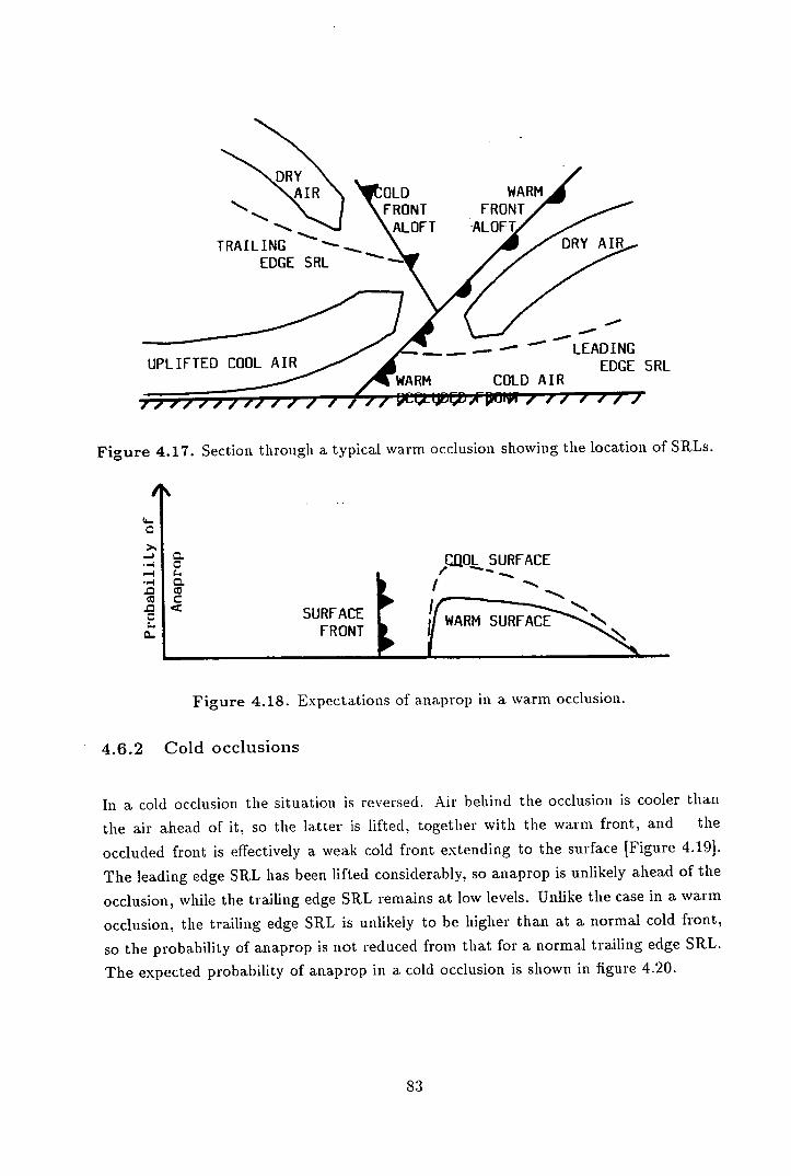
FRONT N.ALOFT
TRAILING ----- EDGE SRL
WARM FRONT/ ALOFT/
DRY Al
- -
LEADING UPLIFTED COOL AIR
EDGE SRL WARM COLD AIR
Figure 4.17. Section through a typical warm occlusion showing the location of SRLs.
>'I CL
.- I 0
•,-4 I C.
C V ( C .0< o SURFACE CL FRONT
CJjOL SURFACE I,
!(URFACEN
Figure 4.18. Expectations of anaprop in a warm occlusion.
4.6.2 Cold occlusions
In a cold occlusion the situation is reversed. Air behind the occlusion is cooler than
the air ahead of it, so the latter is lifted, together with the warm front, and the
occluded front is effectively a weak cold front extending to the surface [Figure 4.19].
The leading edge SRL has been lifted considerably, so anaprop is unlikely ahead of the
occlusion, while the trailing edge SRL remains at low levels. Unlike the case in a warm
occlusion, the trailing edge SRL is unlikely to behigher than at a normal cold front,
so the probability of anaprop is not reduced from that for a normal trailing edge SRL.
The expected probability of anaprop in a cold occlusion is shown in figure 4.20.
83
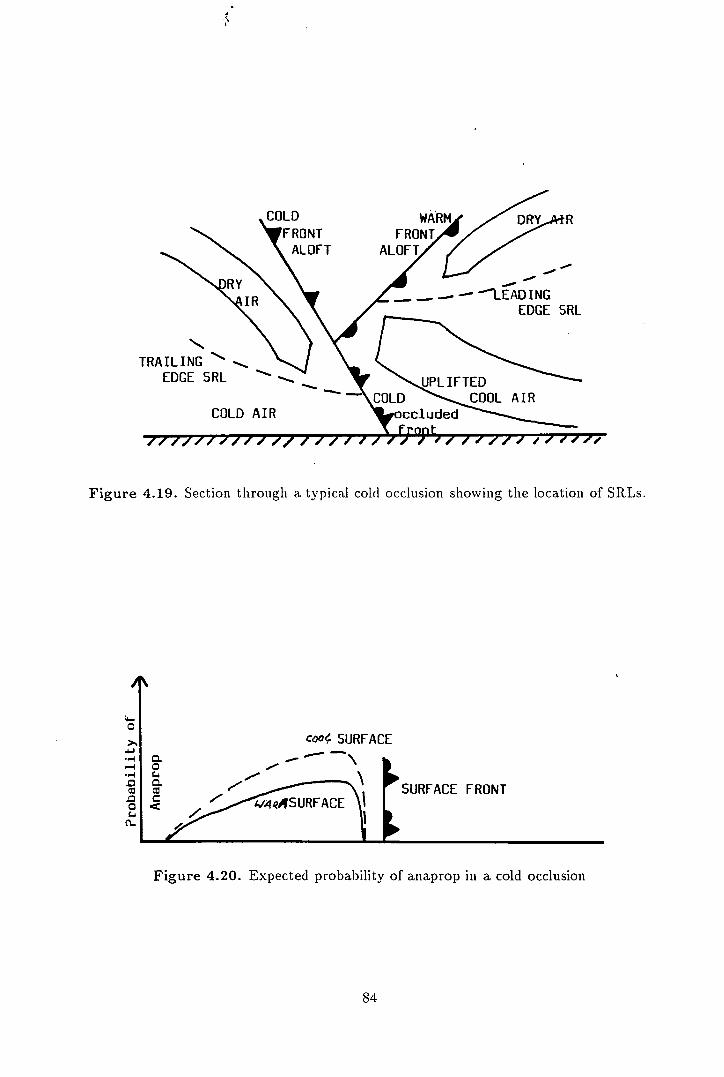
/FRONT DRY R COLD
TALOFT
~I \R 'LEADING EDGE SRL
TRAILING •• ._.
EDGE SRL UPLIFTED COLD COOL AIR
COLD AIR uded
Figure 4.19. Section through a typical cold occlusion showing the location of SRLs.
F. >j coo SURFACE
.1-31
..-Il 0.
.010.
ZASCE\ SURFACE FRONT
/ CLI
Figure 4.20. Expected probability of anaprop in a cold occlusion
84
4.6.3 Discussion
Since the SRLs associated with both types of occlusion are narrow, the path/front
geometry is important when considering anaprop. As usual, long range propagation is
possible when signals are transmitted parallel to the front.
4.7 Warm sector subsidence
As discussed earlier [Chapter 21, cases of very severe anaprop have been observed when
a signal path is in the warm sector of a depression as it skirts the edge of a high. For this
reason, the statistical analysis investigated the interactions of fronts and anticyclones
and found that, though rare, they gave rise to above average quantities of anaprop.
Initially termed 'sporadic subsidence' by BTL [Hewitt et.a.i. 1981, Bye 1988a], these
periods of anaprop appear to occur in the warm sector of a depression and have been
renamed 'warm sector subsidence' in this work.
Warm sector subsidence can be considered to he an extreme example of the models of
kata-fronts presented here. The large scale subsidence associated with the high pressure
system brings the frontal SR.Ls down to low levels, leading to higher probabilities of
anaprop. The dry, warm descending air will increase the strength of the inversion,
giving a bigger refractivity lapse rate and thus higher signal levels.
With the overall subsidence, the fronts will almost certainly be kata-type, since the
vigourous ascent at ana-fronts will not occur. It is unclear whether upper cold fronts
will occur, but it is likely that they will when potential instability is great enough.
It appears that warm sector subsidence is an extreme example of frontal anaprop, and
can be explained in terms of the mechanisms identified in this chapter. This helps
to confirm the statistical links hypothesized between frontal and anticyclonic-frontal
conditions in the previous chapter.
85

Chapter 5
Refractivity analysis
I FRONTS'87
One of the most detailed studies of fronts in the last decade was the FRONTS'87
project. This was a series of intensive studies, made by the UK Met Office and the
French Meteorological Service, of depressions approaching the south west of England.
Data from these studies were made available to the author and have been used to
develop and verify the conceptual models presented in the preceding chapter.
This chapter begins with an overview of the project, looking at some of the reasons it
was undertaken and at the data it has produced. This is followed by a discussion of
the studies selected to verify the models and the data which have been used.
Three case studies follow—of ana and kata cold fronts and of an occlusion. These allow
most aspects of the conceptual models to be verified, with the exception of warm fronts
(although these are, to a certain extent, considered with occlusions). In each case an
attempt is made to partially quantify the qualitative models.
5.1 The FRONTS'87 Project
The FRONTS'87 project has provided some of the most detailed studies of fronts in
recent years. It forms the observational element of the Mesoscale Frontal Dynamics
Project (MFDP), which, in turn, forms the British contribution to a larger European
programme on mesoscale meteorology [dough 1987, Clough & Testud 1988]. The
86
MFDP has three specific objectives [ibid.]:
. To obtain an improved dynamical understanding of synoptic, mesoscale and
smaller-scale interactions within cold-frontal systems.
. To acquire mesoscale data sets and use them- for the further development of
numerical models.
. To describe the structure and evolution of mesoscale features in cold fronts and
to derive conceptual models of value in nowcasting.
Preparations for the projects began in 1985, and the observations were made during
the winter of 1987-8, with a full analysis of the results expected to take several more
years.
5.1.1 The field experiment
As stated above, FRONTS'87 was the field experiment to provide data for the MFDP.
It was decided to concentrate on fronts approaching the English Channel from the
Atlantic, to make full use of the various sources of data and also to allow dropsondes
to be used over as large an area as possible. Use of a sea area also reduced topographic
effects [Clough 1987]. To achieve the aim of studying interactions between different
scales, data had to be obtained at all these scales. This was achieved by defining three
nested zones in the observational area [Fig 5.11:
• An outer zone, covering most of England, Ireland and France. Within this area,
routine observations, supplemented by some extra radiosonde ascents at 6 hourly
intervals, provided the data needed to study the synoptic scale.
• An inner zone, covering south-west England and north-west France. Here a num-
ber of special radiosonde sites, with ascents made every three hours, were set up
to provide mesoscale data. In the western part of this zone an aircraft operations
area was defined. Here the MRF (Meteorological Research Flight) Hercules was
used to provide dropsonde profiles through the front.
• A central area, around a number of radar and sodar installations in Brittany.
Together with surface observations, sonde ascents at 90 minute intervals and air-
borne observations, this area was the main source of data on small scale structures
and processes.
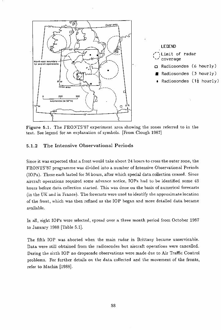
cc 55N
ji Outer area
It
52*
4 North-east boundary tor aircraft operations
Inner area 11
47*N
0 250 500
kilornetres (at 50- N) 0
LEGEND
"iLimit of radar -' coverage
C3 Radiosondes (6 hourly)
I Radiosondes (3 hourly)
• Radiosondes (1 12 hourly)
Figure 5.1. The FRONTS'87 experiment area showing the zones referred to in the text. See legend for an explanation of symbols. [From Clough 1987]
5.1.2 The Intensive Observational Periods
Since it was expected that a front would take about 24 hours to cross the outer zone, the
FRONTS'87 programme was divided into a number of Intensive Observational Periods
(TOPs). These each lasted for 36 hours, after which special data collection ceased. Since
aircraft operations required some advance notice, TOPs had to be identified some 48
hours before data collection started. This was done on the basis of numerical forecasts
(in the UK and in France). The forecasts were used to identify the approximate location
of the front, which was then refined as the lOP began and more detailed data became
available.
In all, eight TOPs were selected, spread over a three month period from October 1987
to January 1988 [Table 5.11.
The fifth TOP was aborted when the main radar in Brittany became unservicable.
Data were still obtained from the radiosondes but aircraft operations were cancelled.
During the sixth TOP no dropsonde observations were made due to Air Traffic Control
problems. For further details on the data collected and the movement of the fronts,
refer to Machin [1988].
88
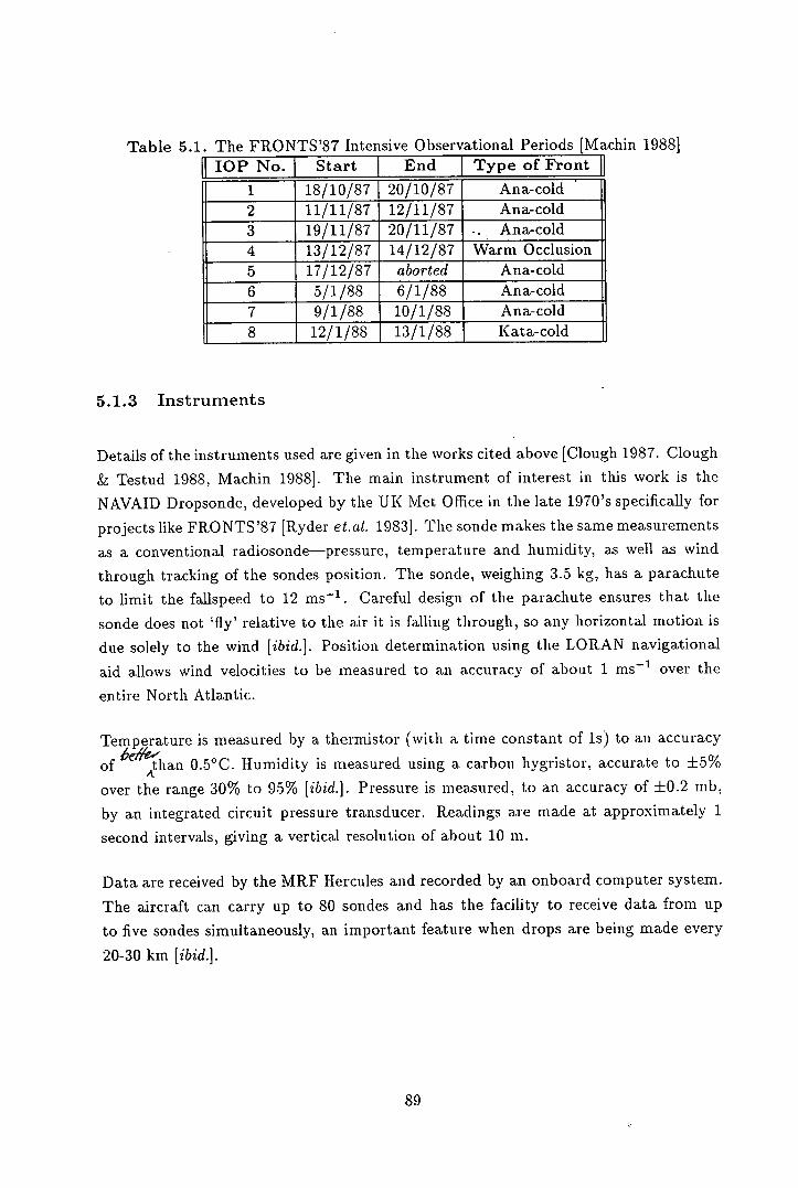
Table 5.1. The FRONTS'87 Intensive Observational Periods [Machin 1988]
lOP No. I Start End [Type of Front
1 18/10/87 20/10/87 Ana-cold
2 11/11/87 12/11/87 Ana-cold
3 19/11/87 20/11/87 . Ana-cold 4 13/12/87 14/12/87 Warm Occlusion
5 17/12/87 aborted Ana-cold
6 5/1/88 6/1/88 Ana-cold
7 9/1/88 10/1/88 Ana-cold
8 12/1/88 13/1/88 Kata-cold
5.1.3 Instruments
Details of the instruments used are given in the works cited above [Clough 1987. Clough
& Testud 1988, Machin 1988]. The main instrument of interest in this work is the
NAVAID Dropsonde, developed by the UK Met Office in the late 1970's specifically for
projects like FRONTS'87 [Ryder et.al . 1983]. The sonde makes the same measurements
as a conventional radiosonde—pressure, temperature and humidity, as well as wind
through tracking of the sondes position. The sonde, weighing 3.5 kg, has a parachute
to limit the fallspeed to 12 ms -1 . Careful design of the parachute ensures that the
sonde does not 'fly' relative to the air it is falling through, so any horizontal motion is
due solely to the wind [ibid.]. Position determination using the LORAN navigational
aid allows wind velocities to be measured to an accuracy of about 1 ms -1 over the
entire North Atlantic
Temperature is measured by a thermistor (with a time constant of is) to an accuracy
of 'han 0.5"C. Humidity is measured using a carbon hygristor, accurate to ±5%
over the range 30% to 95% [ibid.]. Pressure is measured, to an accuracy of ±0.2 mb,
by an integrated circuit pressure transducer. Readings are made at approximately 1
second intervals, giving a vertical resolution of about 10 m.
Data are received by the MRF Hercules and recorded by an onboard computer system.
The aircraft can carry up to 80 sondes and has the facility to receive data from up
to five sondes simultaneously, an important feature when drops are being made every
20-30 km [ibid.].
89
5.2 Radio-Meteorological Studies
Since the MFDP did not examine the refractivity structure of the. FRONTS'87 data,
the Met Office were happy to supply Edinburgh University with the entire FRONTS'87
dataset for refractivity research'. The dataset included dropsondes, radiosondes and
mesoscale model data, but it was decided at the beginning that the dropsonde data
should be the primary source. To study the widest possible range of conditions, three
lOPs were selected for analysis. These were:
. lOP 7, to examine an ana-type (rearwards sloping) cold front.
. lOP 8, to examine a kata-type (split, or forwards sloping) cold front.
. lOP 4, to examine an occlusion and, to a lesser extent, a warm front.
No studies were possible for lOPs 5 and 6, since no dropsonde observations were made,
and lOPs 1-3 had less data available than lOP 7, so they were rejected as ana-front
studies.
5.2.1 Data Processing
All the data were supplied on magnetic tape which was read into the Edinburgh Uni-
versity EMAS system and then transferred to the Meteorology Department's UNIX
network. Data were supplied in a coded format with one file per drop, a total of 206
files from all the TOPs. Initial processing—to extract height, pressure, temperature
and humidity—was then carried out.
It was initially decided that only four quantities were required for the analysis, to which
a fifth was later added. They are:
. The Potential Refractivity, K, calculated as shown below.
= 77.6- + 3.73 x 10 -"0 (5.1)
where 9 is the potential temperature (defined in equation 5.7).
e0 = e(10001P) (P is the pressure in mb) and e is given by:
'The author would like to take this opportunity to thank Drs S Clough and 3 McKay for their help in supplying and decoding the data. Without their assistance none of the FRONTS'87 work would have been possible.
90
( 17.27T e 3 = 6.11 exp
T + 237.3) - (5.2)
('c/ens 193oJ ohe T; ,1 0
and
e = Ue3 1100 (5.3)
Potential refractivity is the main quantity usedto verify the conceptual models.
The Refractivity, N.
N = 77.6ç + 3.73 x 10-- T 2
where P is the pressure (in mb), T is the temperature (in K) and e is the vapour
pressure in mb (as defined above).
N was chosen to support the potential refractivity structure and also to enable
the strength of the refractivity lapse to be determined.
The Equivalent Potential Temperature, 0e, given by:
= 0 + 2.45r (5.5)
where:
r = x 1000 (5.6) 8 p
This was seen as the main way of locating fronts, since they are zones of rapid
change in O.
. The Potential Temperature, 9, given by:
9 = T (2)0.286
This was seen as support for the 0e structure.
The Dewpoint Depression, T - Td, where Td is given by:
Td= 237.3a
1—of
c— ln(j)
17.27
This quantity was selected to aid in the location of fronts by indicating the loca-
tion of clouds and dry air.
The distance of each drop along the run was calculated from the plots given by Machin
[1988], with positions accurate to ±3km. No account was taken of the movement of the
sondes due to the wind. This was because the horizontal displacements were relatively
(5.4)
and:
(5.7)
(5.8)
(5.9)
91
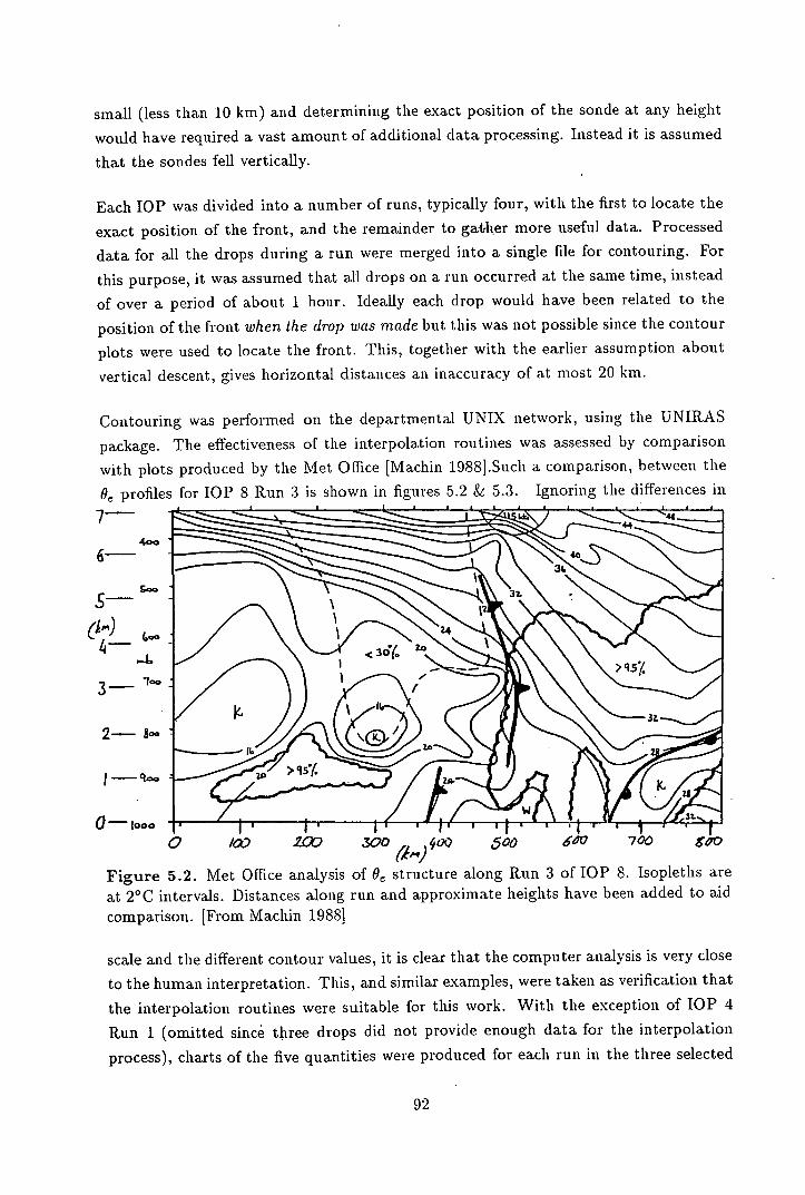
400
6-
500
too
3— Ica
2—Boo
0- 1000
small (less than 10 km) and determining the exact position of the sonde at any height
would have required a vast amount of additional data processing. Instead it is assumed
that the sondes fell vertically.
Each lOP was divided into a number of runs, typically four, with the first to locate the
exact position of the front, and the remainder to gat.her more useful data. Processed
data for all the drops during a run were merged into a single file for contouring. For
this purpose, it was assumed that all drops on a run occurred at the same time, instead
of over a period of about 1 hour. Ideally each drop would have been related to the
position of the front when the drop was made but this was not possible since the contour
plots were used to locate the front. This, together with the earlier assumption about
vertical descent, gives horizontal distances an inaccuracy of at most 20 km.
Contouring was performed on the departmental UNIX network, using the UNIRAS
package. The effectiveness of the interpolation routines was assessed by comparison
with plots produced by the Met Office [Machin 1988].Such a comparison, between the
0 profiles for lOP 8 Run 3 is shown in figures 5.2 & 5.3. Ignoring the differences in
7— i -44
0 ZO.7 300 (AM)
40 500 6t7 700 900
Figure 5.2. Met Office analysis of °e structure along Run 3 of lOP 8. Isopleths are at 2°C intervals. Distances along run and approximate heights have been added to aid comparison. [From Machin 19881
scale and the different contour values, it is clear that the computer analysis is very close
to the human interpretation. This, and similar examples, were taken as verification that
the interpolation routines were suitable for this work. With the exception of lOP 4
Run 1 (omitted since'three drops did not provide enough data for the interpolation
process), charts of the five quantities were produced for each run in the three selected
92
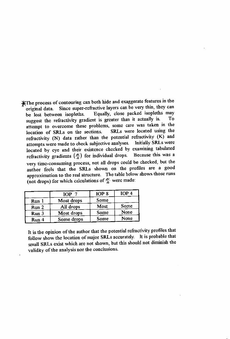
*The process of contouring can both hide and exaggerate features in the original data. Since super-refractive layers can be very thin, they can be lost between isopleths. Equally, close packed isopleths may suggest the refractivity gradient is greater than it actually is. To
attempt to overcome these problems, some care was taken in the location of SRLs on the sections. SRLs were located using the refractivity (N) data rather than the potential refractivity (K) and attempts were made to check subjective analyses. Initially SRLs were located by eye and their existence checked by examining tabulated
refractivity gradients (4) for individual drops. Because this was a
very time-consuming process, not all drops could be checked, but the author feels that the SRLs shown on the profiles are a good approximation to the real structure. The table below shows those runs (not drops) for which calculations of% were made:
______ lOP 7 10P8 10P4
Run 1 Most drops Some
Run 2 Run All drops Most Some
Run 3 Most drops Some None
4 Some drops r Some None
It is the opinion of the author that the potential refractivity profiles that follow show the location of major SRLs accurately. It is probable that small SRLs exist which are not shown, but this should not diminish the validity of the analysis nor the conclusions.
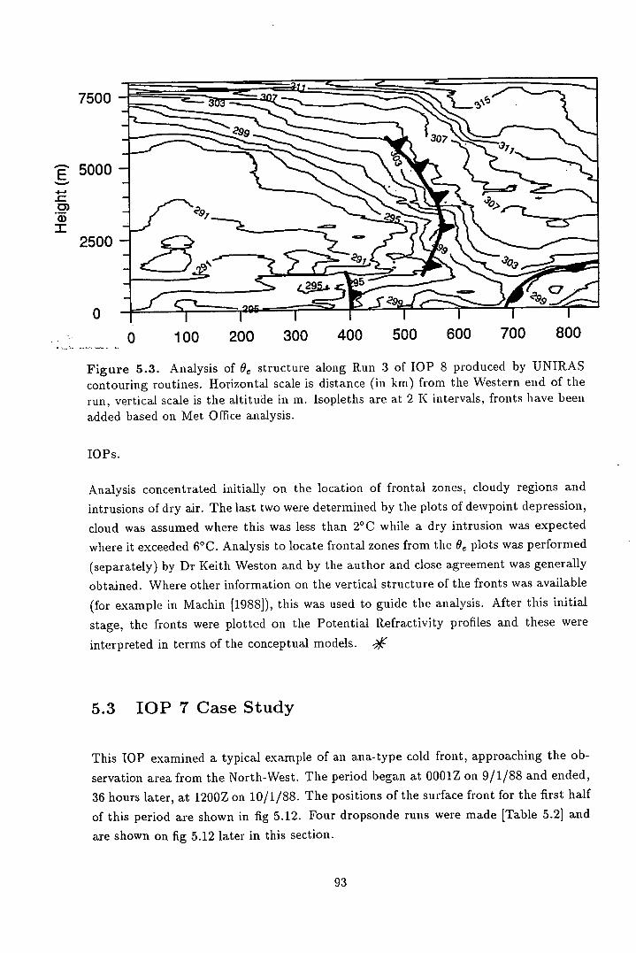
7500
'299 307
5000
0) a) I
2500
N_ 00a
3, A 99
[I]
0 100 200 300 400 500 600 700 800
Figure 5.3. Analysis of O structure along Run 3 of lOP 8 produced by UNIRAS contouring routines. Horizontal scale is distance (in km) from the Western end of the run, vertical scale is the altitude in in. Isopleths are at 2 K intervals, fronts have been
added based on Met Office analysis.
Tops.
Analysis concentrated initially on the location of frontal zones, cloudy regions and
intrusions of dry air. The last two were determined by the plots of dewpoint depression,
cloud was assumed where this was less than 2°C while a dry intrusion was expected
where it exceeded 6°C. Analysis to locate frontal zones from the 0e plots was performed
(separately) by Dr Keith Weston and by the author and close agreement was generally
obtained. Where other information on the vertical structure of the fronts was available
(for example in Machin [1988]), this was used to guide the analysis. After this initial
stage, the fronts were plotted on the Potential Refractivity profiles and these were
interpreted in terms of the conceptual models. -E'
5.3 lOP 7 Case Study
This TOP examined a typical example of an ana-type cold front, approaching the ob-
servation area from the North-West. The period began at 0001Z on 9/1/88 and ended,
36 hours later, at 1200Z on 10/1/88. The positions of the surface front for the first half
of this period are shown in fig 5.12. Four dropsonde runs were made [Table 5.21 and
are shown on fig 5.12 later in this section.
93
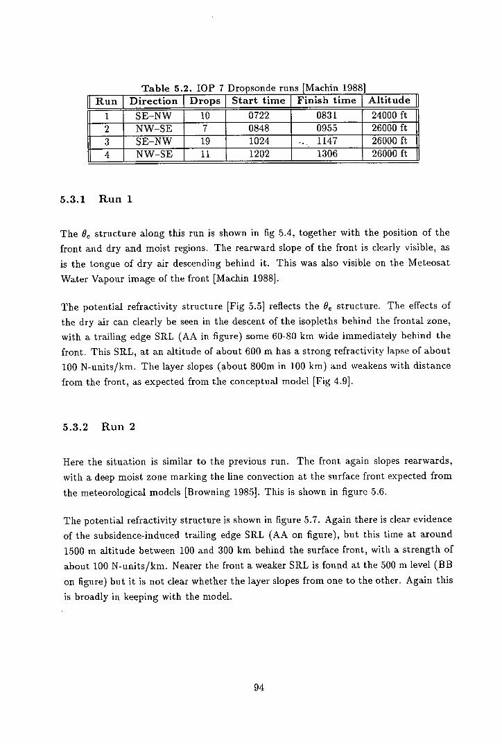
Table 5.2. lOP 7 Dropsonde runs [Machin 1988] [j Run I Direction I Drops I Start time I Finish time I Altitudefi
1 SE—NW 10 0722 0831 24000 ft 2 NW—SE 7 0848 0955 26000 ft
3 SE—NW 19 1024 -. 1147 26000 ft 4 NW—SE 11 1202 1306 26000 ft
5.3.1 Run 1
The Oe structure along this run is shown in fig 5.4, together with the position of the
front and dry and moist regions. The rearward slope of the front is clearly visible, as
is the tongue of dry air descending behind it. This was also visible on the Meteosat
Water Vapour image of the front [Machin 1988].
The potential refractivity structure [Fig 5.5] reflects the 9e structure. The effects of
the dry air can clearly be seen in the descent of the isopleths behind the frontal zone,
with a trailing edge SRL (AA in figure) some 60-80 km wide immediately behind the
front. This SRL, at an altitude of about 600 m has a strong refractivity lapse of about
100 N-units/km. The layer slopes (about 800m in 100 km) and weakens with distance
from the front, as expected from the conceptual model [Fig 4.91.
5.3.2 Run 2
Here the situation is similar to the previous run. The front again slopes rearwards,
with a deep moist zone marking the line convection at the surface front expected from
the meteorological models [Browning 1985]. This is shown in figure 5.6.
The potential refractivity structure is shown in figure 5.7. Again there is clear evidence
of the subsidence-induced trailing edge SRL (AA on figure), but this time at around
1500 m altitude between 100 and 300 km behind the surface front, with a strength of
about 100 N-units/km. Nearer the front a weaker SRL is found at the 500 m level (BB
on figure) but it is not clear whether the layer slopes from one to the other. Again this
is broadly in keeping with the model.
94
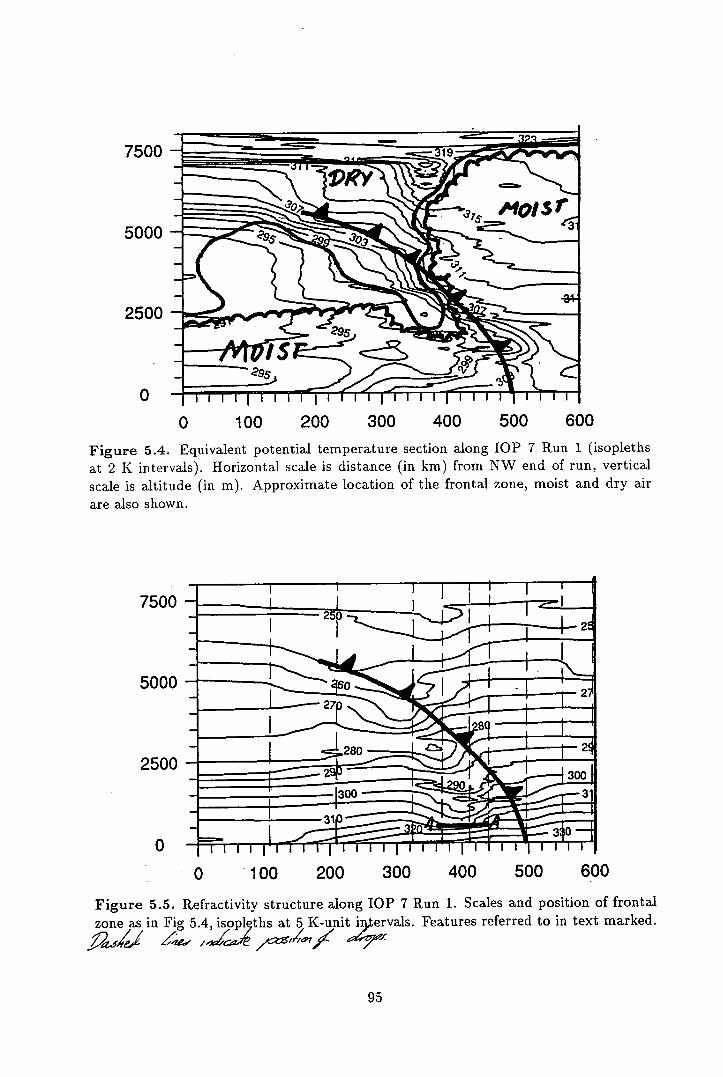
7500
5000
2500
0 100 200 300 400 500 600
Figure 5.4. Equivalent potential temperature section along TOP 7 Run 1 (isopleths at 2 K intervals). Horizontal scale is distance (in km) from NW end of run, vertical scale is altitude (in m). Approximate location of the frontal zone, moist and dry air
are also shown.
7500
5000
2500
0 100 200 300 400 500 600
Figure 5.5. Refractivity structure along TOP 7 Run 1. Scales and position of frontal zone as in Fig 5.4, isopi ths at 5 K-unit i5tervals. Features referred to in text marked.
z€
95
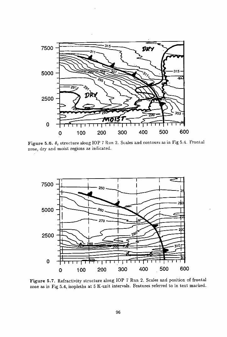
7500
5000
2500
IC
0 100 200 300 400 500 600
Figure 5.6. O structure along lOP 7 Run 2. Scales and contours as in Fig 5.4. Frontal zone, dry and moist regions as indicated.
7500
5000
2500
0 100 200 300 400 500 600
Figure 5.7. Refractivity structure along lOP 7 Run 2. Scales and position of frontal zone as in Fig 5.4, isopleths at 5 K-unit intervals. Features referred to in text marked.
96
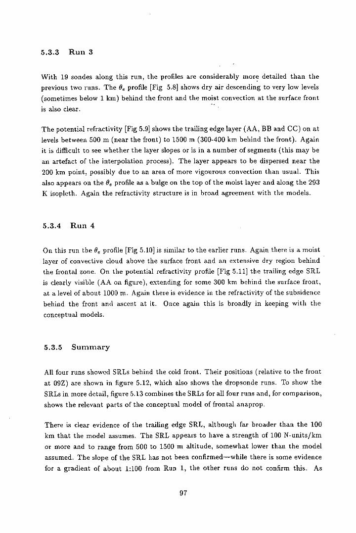
5.3.3 Run 3
With 19 sondes along this run, the profiles are considerably more detailed than the
previous two runs. The 9e profile [Fig 5.8] shows dry air descending to very low levels
(sometimes below 1 km) behind the front and the moist convection at the surface front
is also clear.
The potential refractivity [Fig 5.9] shows the trailing edge layer (AA, BB and CC) on at
levels between 500 m (near the front) to 1500 m (300-400 km behind the front). Again
it is difficult to see whether the layer slopes or is in a number of segments (this may be
an artefact of the interpolation process). The layer appears to be dispersed near the
200 km point, possibly due to an area of more vigourous convection than usual. This
also appears on the °e profile as a bulge on the top of the moist layer and along the 293
K isopleth. Again the refractivity structure is in broad agreement with the models.
5.3.4 Run 4
On this run the 9e profile [Fig 5.10] is similar to the earlier runs. Again there is a moist
layer of convective cloud above the surface front and an extensive dry region behind
the frontal zone. On the potential refractivity profile [Fig 5.11] the trailing edge SRL
is clearly visible (AA on figure), extending for some 300 km behind the surface front,
at a level of about 1000 m. Again there is evidence in the refractivity of the subsidence
behind the front and ascent at it. Once again this is broadly in keeping with the
conceptual models.
5.3.5 Summary
All four runs showed SRLs behind the cold front. Their positions (relative to the front
at 09Z) are shown in figure 5.12, which also shows the dropsonde runs. To show the
SRLs in more detail, figure 5.13 combines the SRLs for all four runs and, for comparison,
shows the relevant parts of the conceptual model of frontal anaprop.
There is clear evidence of the trailing edge SRL, although far broader than the 100
km that the model assumes. The SRL appears to have a strength of 100 N-units/km
or more and to range from 500 to 1500 m altitude, somewhat lower than the model
assumed. The slope of the SRL has not been confirmed—while there is some evidence
for a gradient of about 1:100 from Run 1, the other runs do not confirm this. As
97
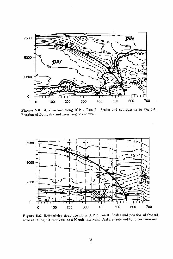
7500
5000
2500
0 100 200 300 400 500 600 700
Figure 5.8. °e structure along lOP 7 Run 3. Scales and contours as in Fig 5.4. Position of front, dry and moist regions shown.
7500
5000
2500
0 100 200 300 400 500 600 700
Figure 5.9. Refractivity structure along TOP 7 Run 3. Scales and position of frontal zone as in Fig 5.4, isopleths at 5 K-unit intervals. Features referred to in text marked.
W.
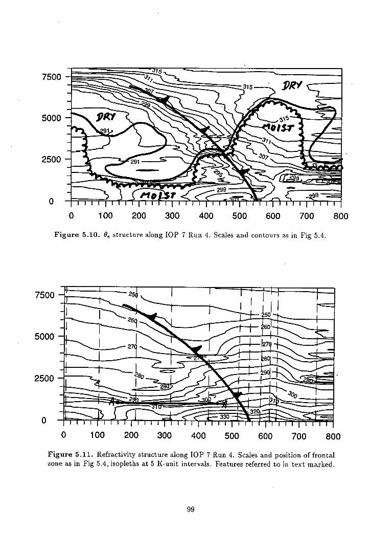
7500
5000
2500
0 100 200 300 400 500 600 700 800
Figure 5.10. °e structure along lOP 7 Run 4. Scales and contours as in Fig 5.4.
r1;1sI
5000
2500
51
0 100 200 300 400 500 600 700 800
Figure 5.11. Refractivity structure along lOP 7 Run 4. Scales and position of frontal zone as in Fig 5.4, isopleths at 5 K-unit intervals. Features referred to in text marked.
99
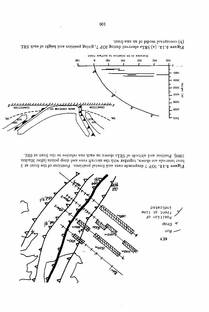
Pa1B 3 TPUT @WT4 qe qUOJJ
.Jo UOTTSO
doa
unJ _-
A 3>
ol
001
uoJJ-u we jo japoux jndalIoD (q)
'fliS pj0 'T!1 pue uo!!sod U!A ' L dOT urp paiasqo S'T3JS () " d
1UOJJ ODBJJflS ol CDAT1BTCDJ W)I Ut 03uBSTJ
O0L 0 00t OOZ ooc ootp ooc
I I I I I -o --
0001
- 000z CD
— 000 17
— 000c
N01133AN03 139 HOA3AN03 WdVN N01133AN03 — 0009
-INS IV HI 'INS 000L
Z60 IT luO.'J 0111 02 aAi2jOJ UflJ UO UMOJ4S s'pJg JO aprijj PITT 110!2!90d •[86T unpw iaje] s2urod doip PUT suni 4j'eJDJI'e alp q2tM ipao ' uMOIIs aJIR sIAJau! J11011
IT 2UOJJ aq JO SUOT2TSOd 5U012!SOdjvquoij pue suni apuosdo.ip L dOT a.inj.
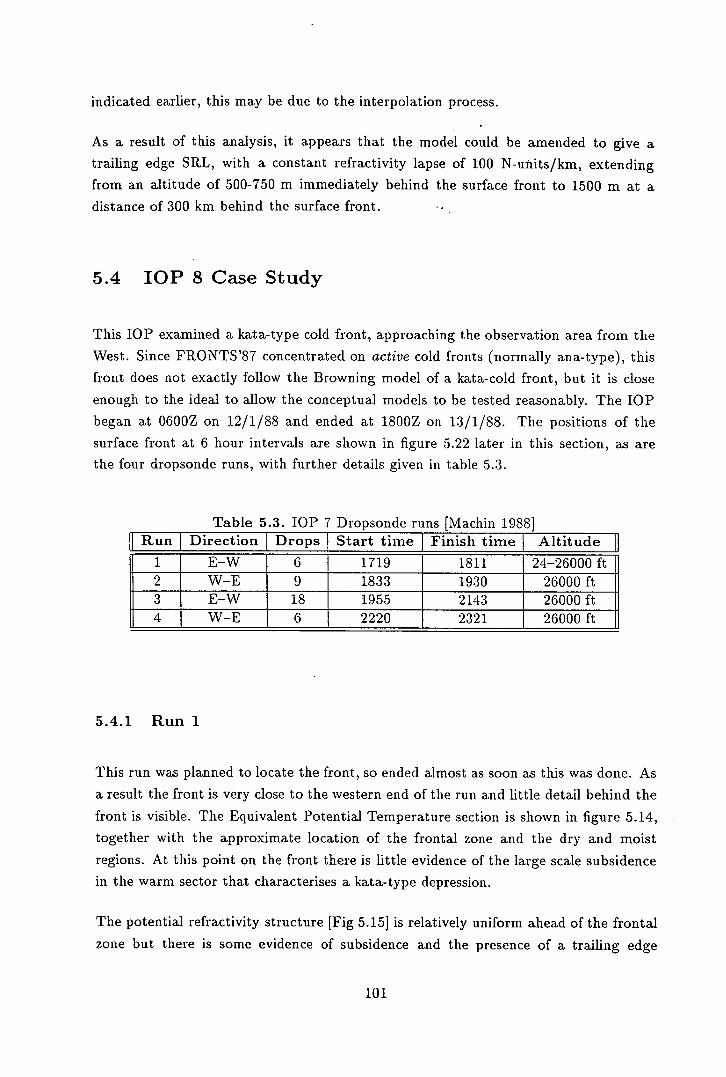
indicated earlier, this may be due to the interpolation process.
As a result of this analysis, it appears that the model could be amended to give a
trailing edge SRL, with a constant refractivity lapse of 100 N-uiiits/km, extending
from an altitude of 500-750 m immediately behind the surface front to 1500 m at a
distance of 300 km behind the surface front.
5.4 lOP 8 Case Study
This lOP examined a kata-type cold front, approaching the observation area from the
West. Since FRONTS'87 concentrated on active cold fronts (normally ana-type), this
front does not exactly follow the Browning model of a kata-cold front, but it is close
enough to the ideal to allow the conceptual models to be tested reasonably. The lOP
began at 0600Z on 12/1/88 and ended at 1800Z on 13/1/88. The positions of the
surface front at 6 hour intervals are shown in figure 5.22 later in this section, as are
the four dropsonde runs, with further details given in table 5.3.
Table 5.3. lOP 7 Dropsonde runs [Machin 19881 [[Run 1 Direction I Drops I Start time I Finish time I Altitude
1 E-W 6 1719 1811 24-26000 ft 2 W-E 9 1833 1930 26000 ft 3 E-W 18 1955 2143 26000 ft 4 W-E 6 2220 2321 26000 ft
5.4.1 Run 1
This run was planned to locate the front, so ended almost as soon as this was done. As
a result the front is very close to the western end of the run and little detail behind the
front is visible. The Equivalent Potential Temperature section is shown in figure 5.14,
together with the approximate location of the frontal zone and the dry and moist
regions. At this point on the front there is little evidence of the large scale subsidence
in the warm sector that characterises a kata-type depression.
The potential refractivity structure [Fig 5.15] is relatively uniform ahead of the frontal
zone but there is some evidence of subsidence and the presence of a trailing edge
101
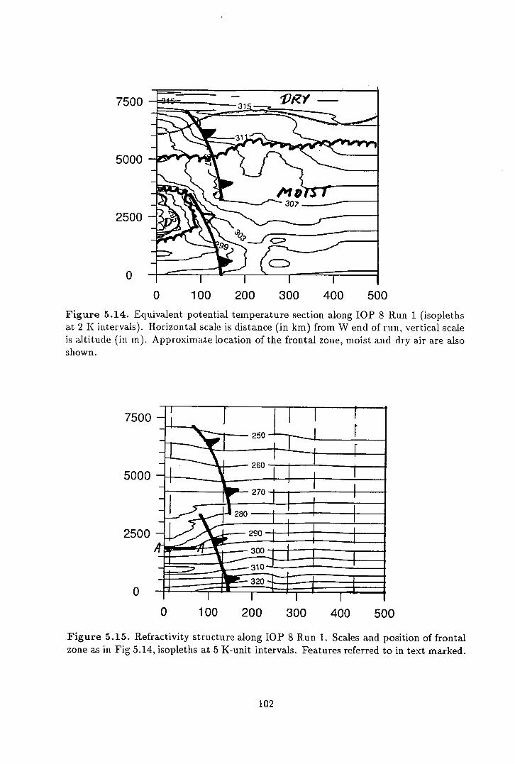
7500
5000
2500
0 100 200 300 400 500
Figure 5.14. Equivalent potential temperature section along lOP 8 Run 1 (isopleths at 2 K intervals). Horizontal scale is distance (in km) from W end of run, vertical scale is altitude (in in). Approximate location of the frontal zone, moist and dry air are also shown.
7500
5000
2500
0 100 200 300 400 500
Figure 5.15. Refractivity structure along lOP 8 Run 1. Scales and position of frontal zone as in Fig 5.14, isopleths at 5 K-unit intervals. Features referred to in text marked.
102
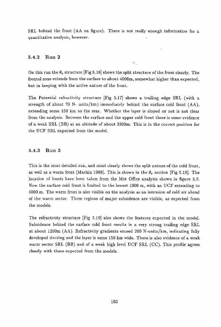
SRL behind the front (AA on figure). There is not really enough information for a
quantitative analysis, however. -
5.4.2 Run 2
On this run the Oe structure [Fig 5.16] shows the split structure of the front clearly. The
frontal zone extends from the surface to about 4000m, somewhat higher than expected,
but in keeping with the active nature of the front.
The Potential refractivity structure [Fig 5.171 shows a trailing edge SRL (with a
strength of about 70 N- units/km) immediately behind the surface cold front (AA),
extending some 150 km to the rear. Whether the layer is sloped or not is not clear
from the analysis. Between the surface and the upper cold front there is some evidence
of a weak SRL (BB) at an altitude of about 3500m. This is in the correct position for
the UCF SRL expected from the model.
5.4.3 Run 3
This is the most detailed run, and most clearly shows the split nature of the cold front,
as well as a warm front [Machin 19881. This is shown in the O section [Fig 5.18]. The
location of fronts have been taken from the Met Office analysis shown in figure 5.2.
Now the surface cold front is limited to the lowest 1000 m, with an UCF extending to
6000 m. The warm front is also visible on the analysis as an intrusion of cold air ahead
of the warm sector. Three regions of major subsidence are visible, as expected from
the models.
The refractivity structure [Fig 5.19] also shows the features expected in the model.
Subsidence behind the surface cold front results in a very strong trailing edge SRL
at about 1200m (AA). Refractivity gradients exceed 200 N-units/km, indicating fully
developed ducting and the layer is some 150 km wide. There is also evidence of a weak
warm sector SRL (BB) and of a weak high level UCF SRL (CC). This profile agrees
closely with those expected from the models.
103
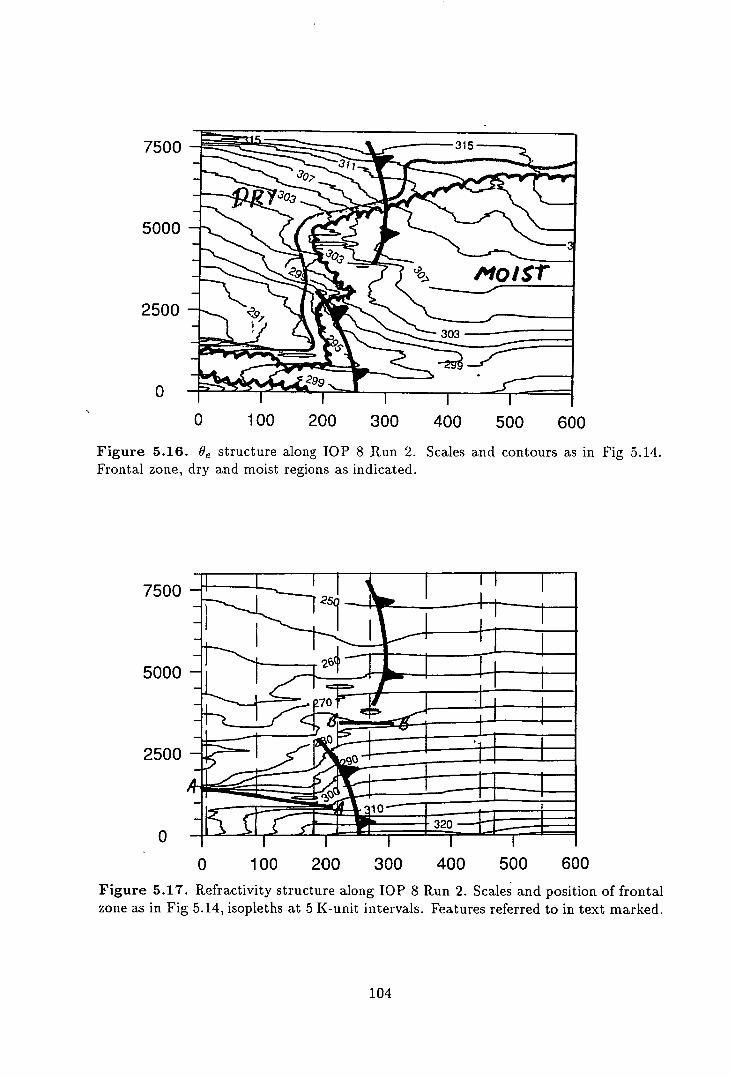
7500
5000
2500
0 100 200 300 400 500 600
Figure 5.16. °e structure along TOP 8 Run 2. Scales and contours as in Fig 5.14. Frontal zone, dry and moist regions as indicated.
7500
5000
2500
[S.]
0 100 200 300 400 500 600
Figure 5.17. Refractivity structure along lOP 8 Run 2. Scales and position of frontal zone as in Fig 5.14, isopleths at 5 K-unit intervals. Features referred to in text marked.
104
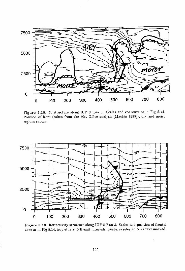
7500
5000
2500
[ii
0 100 200 300 400 500 600 700 800
Figure 5.18. °e structure along lOP 8 Run 3. Scales and contours as in Fig 5.14. Position of front (taken from the Met Office analysis [Machin 1988]), dry and moist regions shown.
7500
5000
2500
0 100 200 300 400 500 600 700 800
Figure 5.19. Refractivity structure along lOP 8 Run 3. Scales and position of frontal zone as in Fig 5.14, isopleths at 5 K-unit intervals. Features referred to in text marked.
105
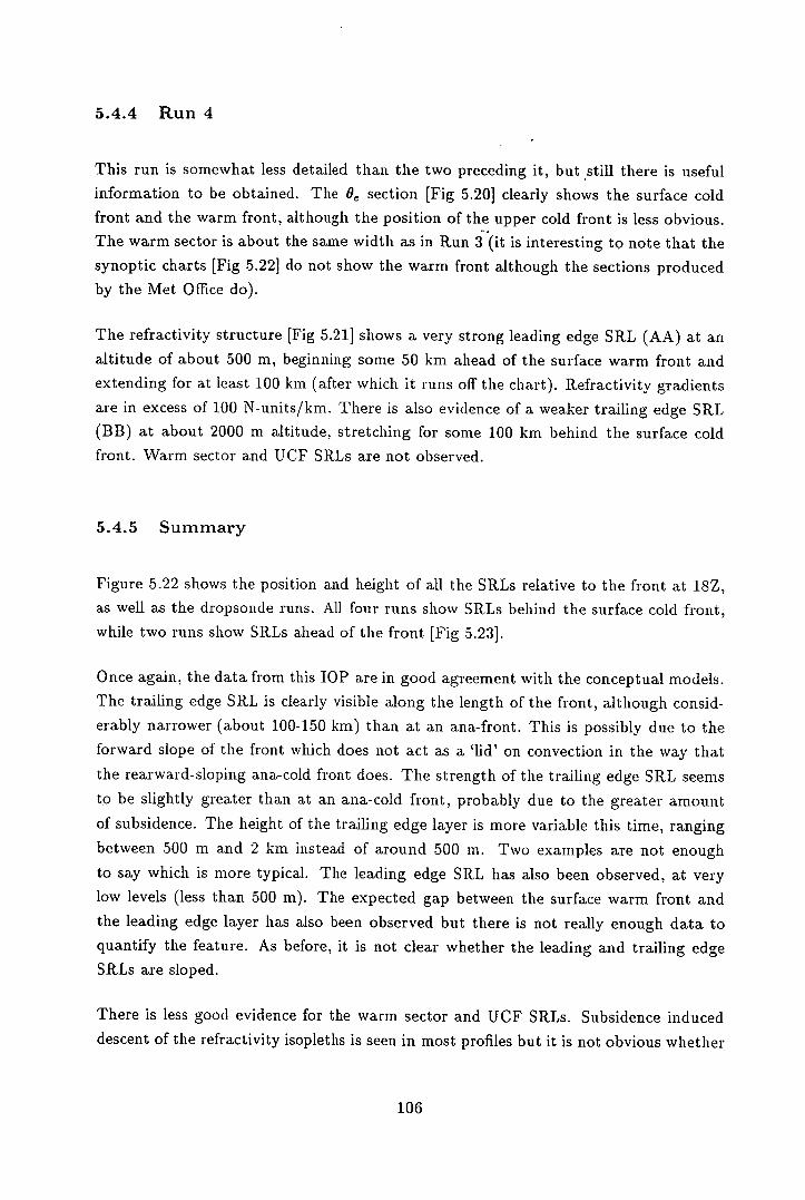
5.4.4 Run 4
This run is somewhat less detailed than the two preceding it, but still there is useful
information to be obtained. The 9 section [Fig 5.20] clearly shows the surface cold
front and the warm front, although the position of the upper cold front is less obvious.
The warm sector is about the same width as in Run 3 (it is interesting to note that the
synoptic charts [Fig 5.22] do not show the warm front although the sections produced
by the Met Office do).
The refractivity structure [Fig 5.211 shows a very strong leading edge SRL (AA) at an
altitude of about 500 m, beginning some 50 km ahead of the surface warm front and
extending for at least 100 km (after which it runs off the chart). Refractivity gradients
are in excess of 100 N-units/km. There is also evidence of a weaker trailing edge SRL
(BB) at about 2000 m altitude, stretching for some 100 km behind the surface cold
front. Warm sector and UCF SRLs are not observed.
5.4.5 Summary
Figure 5.22 shows the position and height of all the SRLs relative to the front at 18Z,
as well as the dropsonde runs. All four runs show SRLs behind the surface cold front,
while two runs show SRLs ahead of the front [Fig 5.23].
Once again, the data from this TOP are in good agreement with the conceptual models.
The trailing edge SRL is clearly visible along the length of the front, although consid-
erably narrower (about 100-150 km) than at an ana-front. This is possibly due to the
forward slope of the front which does not act as a 'lid' on convection in the way that
the rearward-sloping ana-cold front does. The strength of the trailing edge SRL seems
to be slightly greater than at an ana-cold front, probably due to the greater amount
of subsidence. The height of the trailing edge layer is more variable this time, ranging
between 500 m and 2 km instead of around 500 m. Two examples are not enough
to say which is more typical. The leading edge SRL has also been observed, at very
low levels (less than 500 m). The expected gap between the surface warm front and
the leading edge layer has also been observed but there is not really enough data to
quantify the feature. As before, it is not clear whether the leading and trailing edge
SRLs are sloped.
There is less good evidence for the warm sector and TJCF SRLs. Subsidence induced
descent of the refractivity isopleths is seen in most profiles but it is not obvious whether
106
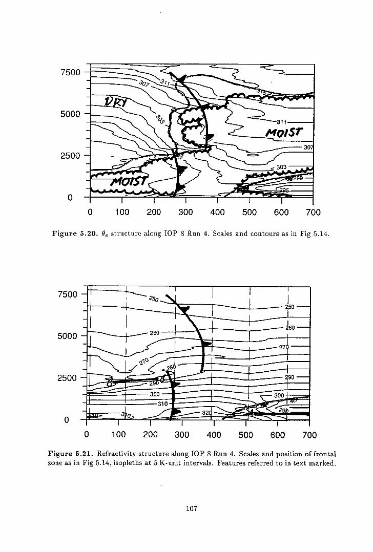
7500
5000
2500
Ell
0 100 200 300 400 500 600 700
Figure 5.20. 9 structure along lOP 8 Run 4. Scales and contours as in Fig 5.14.
7500
5000
2500
iJ
0 100 200 300 400 500 600 700
Figure 5.21. Refractivity structure along lOP 8 Run 4. Scales and position of frontal zone as in Fig 5.14, isopleths at 5 K-unit intervals. Features referred to in text marked.
107
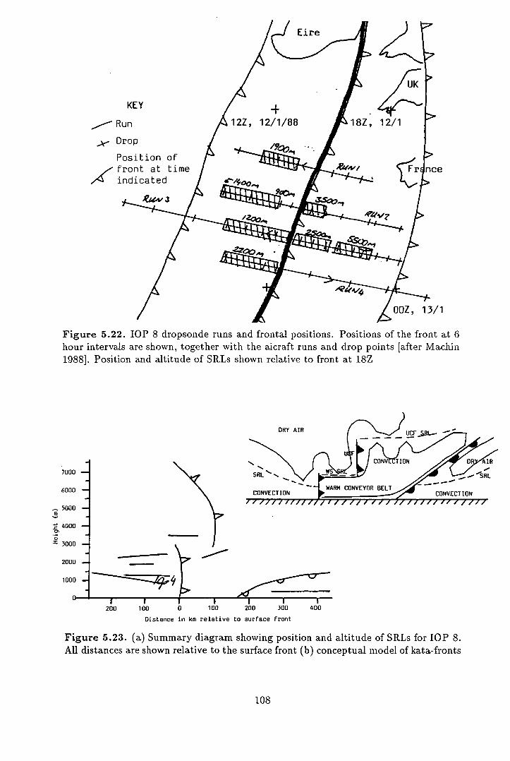
KEY
_- Run ><- Drop
Position of ,— front at time
,4 indicated
.L
Eire
-f 12Z, 12/1/88
72Aq
I18Z
4~ UK
, 12/1
cic
-,t_.____ l•"?
OOZ, 13/1
Figure 5.22. lOP 8 dropsonde runs and frontal positions. Positions of the front at 6 hour intervals are shown, together with the aicraft runs and drop points [after Machin 1988]. Position and altitude of SRLs shown relative to front at 18Z
DRY AIR ( — -- UCF- _5BL-
CON VEtT ION
0 AIR
7000 SRL-.. SRL
6000 CONVECTION _L WARM CONVEYOR
- CONVECTION
5000 - C
4000 -
3000 -
2000
1000 -
200 100 0 100 200 300 400
Distance in km relative to surface front
Figure 5.23. (a) Summary diagram showing position and altitude of SRLs for lOP 8. All distances are shown relative to the surface front (b) conceptual model of kata-fronts
108
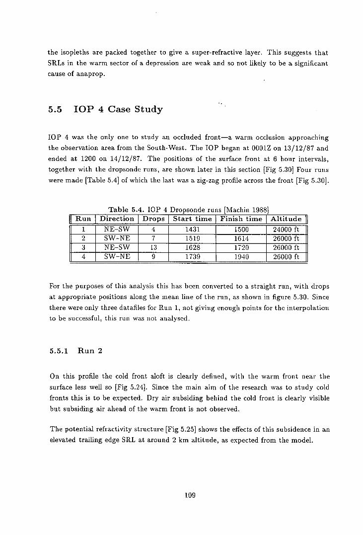
the isopleths are packed together to give a super-refractive layer. This suggests that
SRLs in the warm sector of a depression are weak and so not likely to be a significant
cause of anaprop.
5.5 lOP 4 Case Study
lOP 4 was the only one to study an occluded front—a warm occlusion approaching
the observation area from the South-West. The TOP began at 0001Z on 13/12/87 and
ended at 1200 on 14/12/87. The positions of the surface front at 6 hour intervals,
together with the dropsonde runs, are shown later in this section [Fig 5.30] Four runs
were made [Table 5.4] of which the last was a zig-zag profile across the front [Fig 5.301.
Table 5.4. lOP 4 Dropsonde runs [Machin 19881 Run I Direction [_Drops I Start time I Finish time _[ Altitude
1 NE–SW 4 1431 1500 24000 ft 2 SW–NE 7 1519 1614 26000 ft 3 NE–SW 13 1628 1720 26000 ft 4 SW–NE 9 1739 1940 26000 ft
For the purposes of this analysis this has been converted to a straight run, with drops
at appropriate positions along the mean line of the run, as shown in figure 5.30. Since
there were only three datafiles for Run 1, not giving enough points for the interpolation
to be successful, this run was not analysed.
5.5.1 Run 2
On this profile the cold front aloft is clearly defined, with the warm front near the
surface less well so [Fig 5.24]. Since the main aim of the research was to study cold
fronts this is to be expected. Dry air subsiding behind the cold front is clearly visible
but subsiding air ahead of the warm front is not observed.
The potential refractivity structure [Fig 5.25] shows the effects of this subsidence in an
elevated trailing edge SRL at around 2 km altitude, as expected from the model.
109
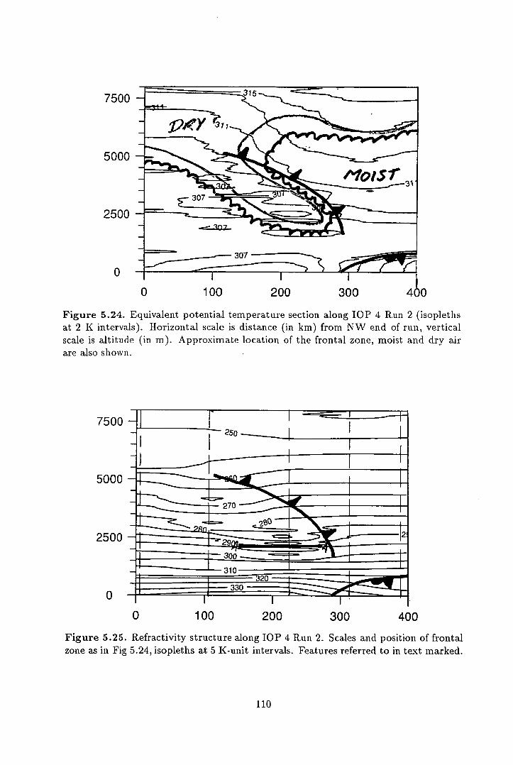
7500
2500
[I]
Figure 5.24. Equivalent potential temperature section along TOP 4 Run 2 (isopleths at 2 K intervals). Horizontal scale is distance (in km) from NW end of run, vertical scale is altitude (in m). Approximate location of the frontal zone, moist and dry air are also shown.
7500
5000
2500
0 100 200 300 400
Figure 5.25. Refractivity structure along lOP 4 Run 2. Scales and position of frontal zone as in Fig 5.24, isopleths at 5 K-unit intervals. Features referred to in text marked.
110
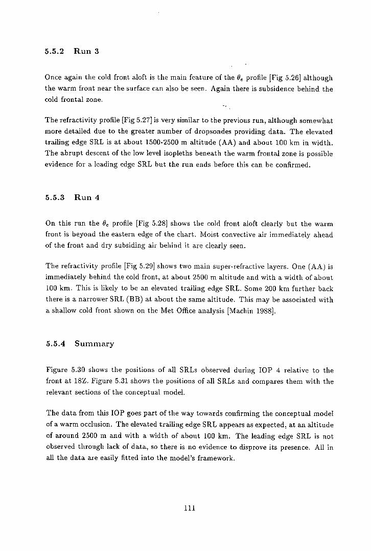
5.5.2 Run 3
Once again the cold front aloft is the main feature of the Oe profile Fig 5.26] although
the warm front near the surface can also be seen. Again there is subsidence behind the
cold frontal zone.
The refractivity profile [Fig 5.27] is very similar to the previous run, although somewhat
more detailed due to the greater number of dropsondes providing data. The elevated
trailing edge SRL is at about 1500-2500 m altitude (AA) and about 100 km in width.
The abrupt descent of the low level isopleths beneath the warm frontal zone is possible
evidence for a leading edge SRL but the run ends before this can be confirmed.
5.5.3 Run 4
On this run the °e profile [Fig 5.28] shows the cold front aloft clearly but the warm
front is beyond the eastern edge of the chart. Moist convective air immediately ahead
of the front and dry subsiding air behind it are clearly seen.
The refractivity profile [Fig 5.29] shows two main super-refractive layers. One (AA) is
immediately behind the cold front, at about 2500 m altitude and with a width of about
100 km. This is likely to be an elevated trailing edge SRL. Some 200 km further back
there is a narrower SRL (BB) at about the same altitude. This may be associated with
a shallow cold front shown on the Met Office analysis [Machin 1988].
5.5.4 Summary
Figure 5.30 shows the positions of all SRLs observed during lOP 4 relative to the
front at 18Z. Figure 5.31 shows the positions of all SRLs and compares them with the
relevant sections of the conceptual model.
The data from this lOP goes part of the way towards confirming the conceptual model
of a warm occlusion. The elevated trailing edge SRL appears as expected, at an altitude
of around 2500 m and with a width of about 100 km. The leading edge SRL is not
observed through lack of data, so there is no evidence to disprove its presence. All in
all the data are easily fitted into the model's framework.
111
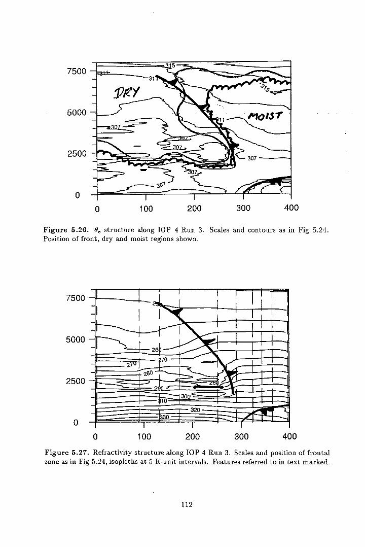
7500
5000
2500
[I]
0 100 200 300 400
Figure 5.26. 9 structure along lOP 4 Run 3. Scales and contours as in Fig 5.24. Position of front, dry and moist regions shown.
7500
5000
2500
sJ 0 100 200 300 400
Figure 5.27. Refractivity structure along lOP 4 Run 3. Scales and position of frontal zone as in Fig 5.24, isopleths at 5 K-unit intervals. Features referred to in text marked.
112
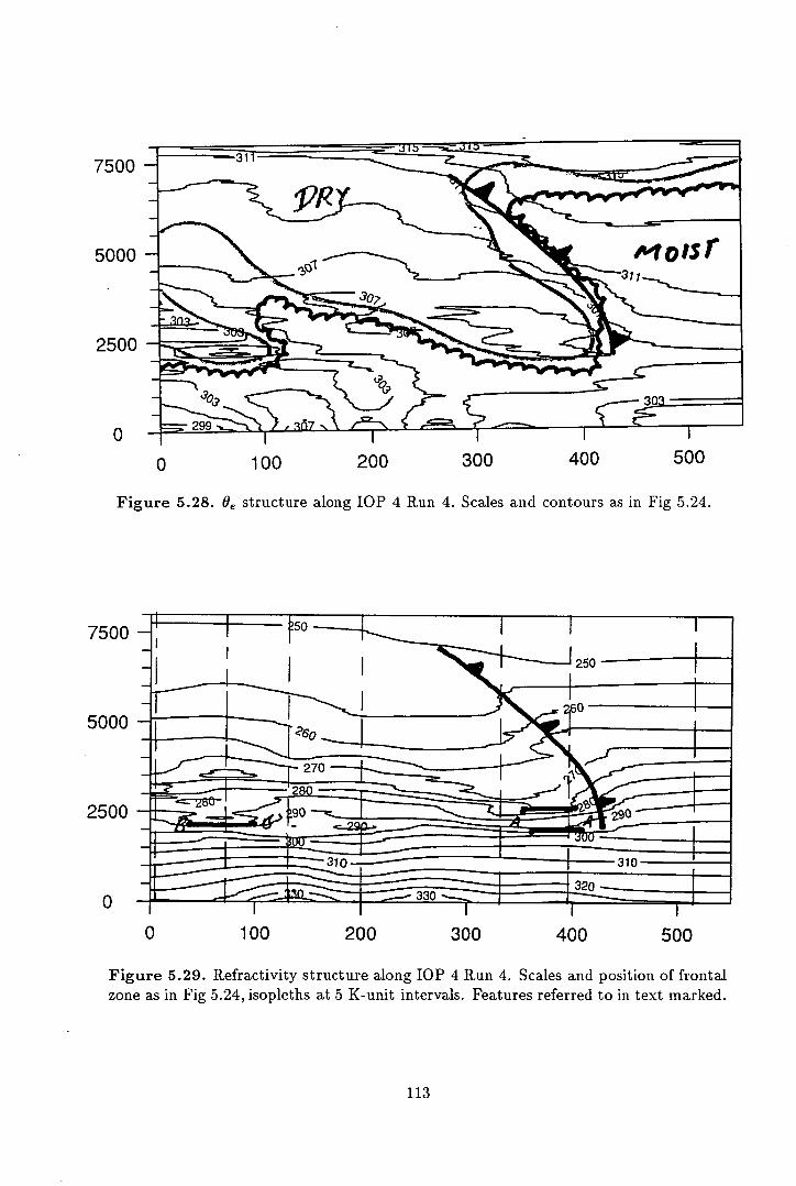
7500
5000
2500
1'•
imcfeTt
0
0 100 200 300 400 500
Figure 5.28. 9 structure along lOP 4 Run 4. Scales and contours as in Fig 5.24.
7500
5000
2500
:i,11___ •-
-Cl',-- -
0
0 100 200 300 400 500
Figure 5.29. Refractivity structure along lOP 4 Run 4. Scales and position of frontal zone as in Fig 5.24, isopleths at 5 K-unit intervals. Features referred to in text marked.
113
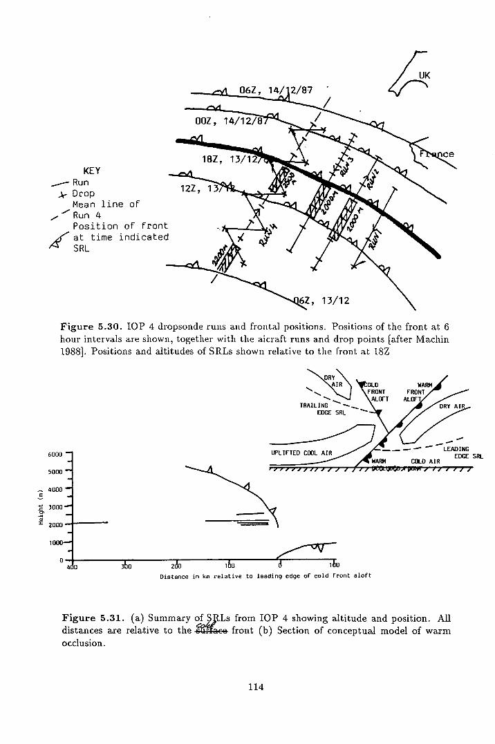
UP
UK
14/12/87 -
KEY __- Run
- Drop Mean line of Run4 Position of front
J' at time indicate( ,A SRL
Figure 5.30. lOP 4 dropsonde runs and frontal positions. Positions of the front at 6 hour intervals are shown, together with the aicraft runs and drop points [after Machin 1988]. Positions and altitudes of SRLs shown relative to the front at 18Z
•• 'AIR OLD \FRON \ALIJ
TRAILING EDGE SRI
6000 1 EDLAIR/
5000
4000
-1 30001
= 2000H
WARN
%AIR
1 SRL
N
0
Distance in km relative to leading edge of cold front aloft
Figure 5.31. (a) Summary of $RLs from lOP 4 showing altitude and position. All distances are relative to the -sufface front (b) Section of conceptual model of warm occlusion.
114
5.6 Discussion
The FRONTS'87 project has proved an invaluable source of data for this research.
The data allows the refractivity structure around cold fronts to be studied in far more
detail than conventional radiosonde ascents would allow, both in the horizontal, with
dropsondes every 20-100 km compared with a minimumof 200 km between radiosondes,
and in the vertical, with readings every 10 m compared with 500-1000 m for smoothed
radiosonde data.
Since the FRONTS'87 project concentrated on the structure of active cold fronts it was
not possible to verify all the models. However, a large amount of evidence supporting
certain features of the conceptual models has been gathered, which goes a long way to
suggest that the other, important, features are indeed correct. The FRONTS'87 data
has also allowed a certain amount of quantification of the (previously only qualitative)
models, although there is still a long way to go on this front.
The main finding from the FRONTS'87 dataset has been confirmation of the existence
of the trailing edge SRL, together with some indications of its height and strength. It
was found that the layer is considerably wider when the front is ana-type than when
a kata-front is present, but the strength remains similar, at about 100 N-units/km,
indicating a strongly super-refractive layer. The difference in width appears to be due
to the rearwards slope of the ana-cold front acting as more of a limit to convection
than the forward sloping kata-cold front. In the latter case only the subsiding air acts
to limit the vertical extent of convection while in the former case both the front and
the subsiding air limit convection.
The study of a kata-cold front failed to show strong warm sector and TJCF SRLs,
although there was evidence for a slightly super-refractive atmosphere. Since the models
did not predict the strength of the layers and also since the front was an 'active' one,
this may be a feature of the front rather than a major flaw in the models. Evidence
supporting a leading edge SRL was seen, with the gap between the layer and the surface
front visible. The study of the occlusion was not able to confirm the presence of a low
level leading edge SRL (due to lack of data). The trailing edge layer was found to be
higher than usual for a cold front, as expected from the models.
As has been mentioned before, the FRONTS'87 analysis has not contradicted any
features in the models, although not all the features have been observed. Possible ex-
tensions to this work would include the analysis of detailed data from other programmes
to study warm fronts and occlusions in greater detail.
115

Chapter 6
Refractivity analysis II Gt
Baddow
Although the previous chapter [5] has provided much evidence supporting the con-
ceptual models of frontal radio-meteorology [chapter 4], there has not yet been any
examination of the signals produced when a front intersects a path. This chapter at-
tempts to remedy that. Detailed signal data have been obtained for an experimental
path in south east England, together with routine surface and upper air observations.
This has provided the information for an extended case study of signals and weather
for a three month period in summer 1989. Two types of analysis have been made:
A simple correlation of time series signal data with the position of the surface
front as it approaches, crosses and recedes from the path.
• A more detailed comparison of signal time series with potential refractivity pro-
files derived from radiosonde ascents.
Use of routine weather observations to identify periods of frontal anaprop was of lead to
ways of using forecast data (either surface or upper air) to make short range predictions
of ana.prop associated with fronts.
The chapter begins with a survey of the signal path, the meteorological data available
and some of the reasons for the choice of path and dates. This is followed by a short
examination of the data processing. The signals produced by different types of fronts
are considered in an attempt to find characteristic 'signatures' of frontal anaprop.
Finally some examples of refractivity sections and their relation to signals are examined
116
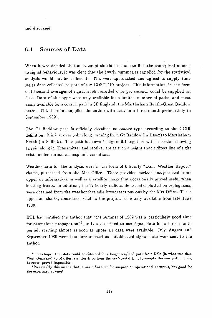
and discussed.
6.1 Sources of Data
When it was decided that an attempt should be made to link the conceptual models
to signal behaviour, it was clear that the hourly summaries supplied for the statistical
analysis would not be sufficient. BTL were approached and agreed to supply time
series data collected as part of the COST 210 project. This information, in the form
of .10 second averages of signal levels recorded once per second, could be supplied on
disk. Data of this type were only available for a limited number of paths, and most
easily available for a coastal path in SE England, the Martiesham Heath—Great Baddow
path'. BTL therefore supplied the author with data for a three month period (July to
September 1989).
The Gt Baddow path is officially classified as coastal type according to the CCIR
definition. It is just over 66km long, running from Gt Baddow (in Essex) to Martlesham
Heath (in Suffolk). The path is shown in figure 6.1 together with a section showing
terrain along it. Transmitter and receiver are at such a height that a direct line of sight
exists under normal atmospheric conditions.
Weather data for the analysis were in the form of 6 hourly "Daily Weather Report"
charts, purchased from the Met Office. These provided surface analyses and some
upper air information, as well as a satellite image that occasionally proved useful when
locating fronts. In addition, the 12 hourly radiosonde ascents, plotted on tephigrams,
were obtained from the weather facsimile broadcasts put out by the Met Office. These
upper air charts, considered vital to the project, were only available from late June
1989.
BTL had notified the author that 'the summer of 1989 was a particularly good time
for anomalous propagation" 2 , so it was decided to use signal data for a three month
period, starting almost as soon as upper air data were available. July, August and
September 1989 were therefore selected as suitable and signal data were sent to the
author.
'It was hoped that data could be obtained for a longer sea/land path from Köln (in what was then West Germany) to Martlesham Heath or from the sea/coastal Eindhoven—Martlesham path. This, however, proved impossible.
2 Presumably this means that it was a bad time for anaprop on operational networks, but good for the experimental ones!
117
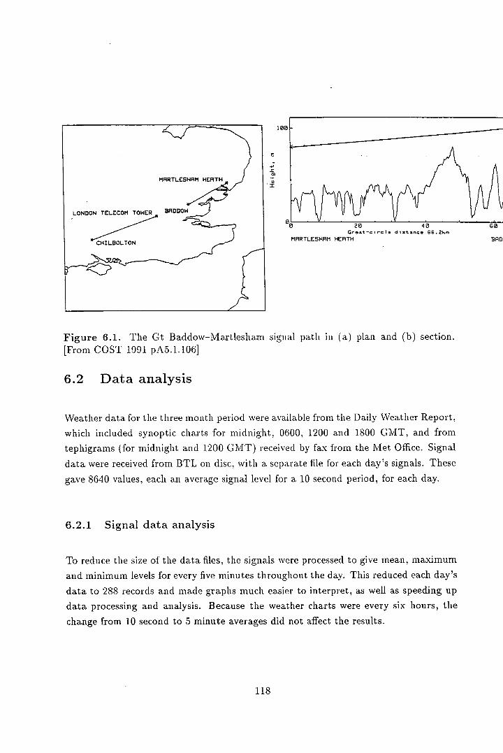
MARTLESHAM HERTH
LONDON TELECOM TOWER BRODOW
CHILBOLTON
0 I
lot
G.-t-ci,c. dtnc 66.2k.,
MRRTLESHAM HEATH BAD:
Figure 6.1. The Ct Baddow-Martlesham signal path in (a) plan and (h) section. [From COST 1991 pA5.1.106]
6.2 Data analysis
Weather data for the three month period were available from the Daily Weather Report,
which included synoptic charts for midnight, 0600, 1200 and 1800 GMT, and from
tephigrams (for midnight and 1200 GMT) received by fax from the Met Office. Signal
data were received from BTL on disc, with a separate file for each day's signals. These
gave 8640 values, each an average signal level for a 10 second period, for each day.
6.2.1 Signal data analysis
To reduce the size of the data files, the signals were processed to give mean, maximum
and minimum levels for every five minutes throughout the day. This reduced each day's
data to 288 records and made graphs much easier to interpret, as well as speeding up
data processing and analysis. Because the weather charts were every six hours, the
change from 10 second to 5 minute averages did not affect the results.
118
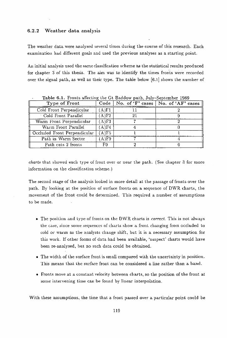
6.2.2 Weather data analysis
The weather data were analysed several times during the course of this research. Each
examination had different goals and used the previous analyses as a starting point.
An initial analysis used the same classification scheme as the statistical results produced
for chapter 3 of this thesis. The aim was to identify the times fronts were recorded
over the signal path, as well as their type. The table below [6.1] shows the number of
Table 6.1. Fronts affecting the Gt Baddow path, July—September 1989 Type of Front [ Code I No. of 'F' cases I No. of 'AF' cases
Cold Front Perpendicular (A)F1 11 2 Cold Front Parallel (A)F2 21 9
Warm Front Perpendicular (A)F3 7 2 Warm Front Parallel (A)F4 4 0
Occluded Front Perpendicular (A)F5 1 1 Path in Warm Sector (A)F9 7 4
Path cuts 2 fronts FO 2 0
charts that showed each type of front over or near the path. (See chapter 3 for more
information on the classification scheme.)
The second stage of the analysis looked in more detail at the passage of fronts over the
path. By looking at the position of surface fronts on a sequence of DWR charts, the
movement of the front could be determined. This required a number of assumptions
to be made.
• The position and type of fronts on the DWR charts is correct. This is not always
the case, since some sequences of charts show a front changing from occluded to
cold or warm as the analysts change shift, but it is a necessary assumption for
this work. If other forms of data had been available, 'suspect' charts would have
been re-analysed, but no such data could he obtained.
• The width of the surface front is small compared with the uncertainty in position.
This means that the surface front can be considered a line rather than a band.
• Fronts move at a constant velocity between charts, so the position of the front at
some intervening time can be found by linear interpolation.
With these assumptions, the time that a front passed over a particular point could be
119
found to a reasonable degree of accuracy'. This allowed fronts to be marked on the
signal level charts, either as a time the front moved from one side of the path to the
other (for fronts parallel to the path) or as the time it reached each end of the path
(for fronts perpendicular to the path).
A further stage of analysis was used for the more detailed cross-section studies. As
well as information from surface charts, tephigrams were used to produce refractivity
sections, both in time and in space. Because of the small scale and poor quality of
the tephigrams, it was not possible to read temperatures or dewpoints to an accuracy
better than ±1°C, nor pressures (except at standard pressure levels) to better than
±10mb. Calculated refractivities were therefore accurate to ±5 K-units [section 2.21.
Using synoptic charts as guides to the type and location of fronts, the refractivity
sections were contoured by hand.
6.3 Correlation of surface data with signals
Once the position and motion of fronts had been established, they were correlated with
the signal charts. This detailed analysis looked at three types of fronts.
. Cold fronts parallel to the signal path
. Cold fronts perpendicular to the signal path
. Warm fronts in any orientation
These categories are a reflection of the number of fronts of each type, and each will be
examined separately.
The aim of this analysis was to (if possible) identify patterns of signal behaviour which
could be considered a 'signature' of frontal anaprop of different types, and also to
identify features of surface observations and synoptic charts which could he used to
predict which fronts would cause anaprop.
3 Reasonable is not easy to define, and depends on individual cases, but it has been assumed for the rest of this chapter that times of passage are accurate to ±1 hour.
120
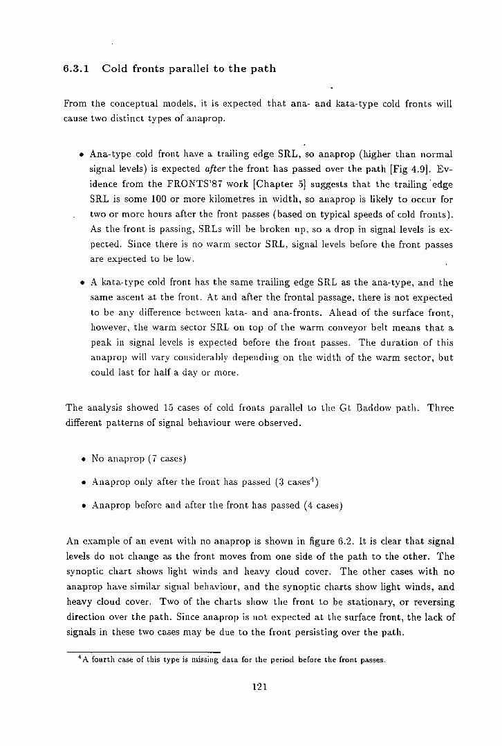
6.3.1 Cold fronts parallel to the path
From the conceptual models, it is expected that ana- and kata-type cold fronts will
cause two distinct types of anaprop.
• Ana-type cold front have a trailing edge SRL, so anaprop (higher than normal
signal levels) is expected after the front has passed over the path [Fig 4.9]. Ev-
idence from the FRONTS'87 work [Chapter 51 suggests that the trailing 'edge
SRL is some 100 or more kilometres in width, so anaprop is likely to occur for
two or more hours after the front passes (based on typical speeds of cold fronts).
As the front is passing, SRLs will he broken up, so a drop in signal levels is ex-
pected. Since there is no warm sector SRL, signal levels before the front passes
are expected to be low.
• A kata-type cold front has the same trailing edge SRL as the ana-type, and the
same ascent at the front. At and after the frontal passage, there is not expected
to be any difference between kata- and ana-fronts. Ahead of the surface front,
however, the warm sector SilL on top of the warm conveyor belt means that a
peak in signal levels is expected before the front passes. The duration of this
anaprop will vary considerably depending on the width of the warm sector, but
could last for half a clay or more.
The analysis showed 15 cases of cold fronts parallel to the Gt Baddow path. Three
different patterns of signal behaviour were observed.
• No anaprop 0 cases)
• Anaprop only after the front has passed (3 cases 4)
• Anaprop before and after the front has passed (4 cases)
An example of an event with no anaprop is shown in figure 6.2. It is clear that signal
levels do not change as the front moves from one side of the path to the other. The
synoptic chart shows light winds and heavy cloud cover. The other cases with no
anaprop have similar signal behaviour, and the synoptic charts show light winds, and
heavy cloud cover. Two of the charts show the front to be stationary, or reversing
direction over the path. Since anaprop is not expected at the surface front, the lack of
signals in these two cases may be due to the front persisting over the path.
4 A fourth case of this type is missing data for the period before the front passes.
121
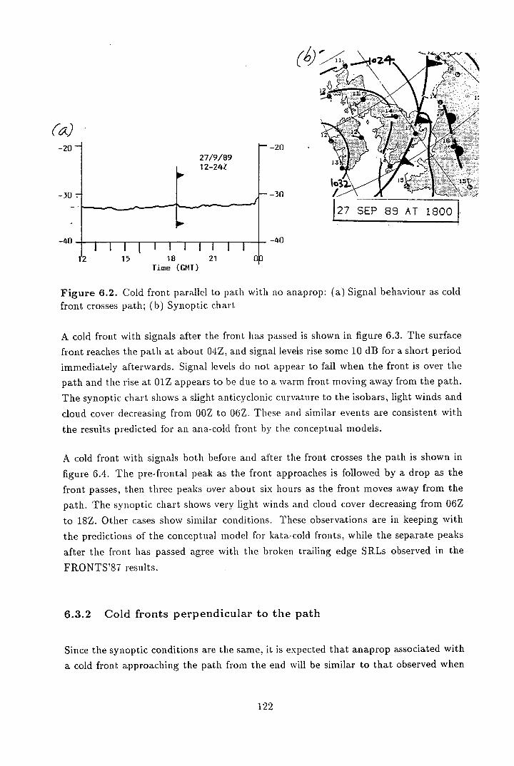
()
-20
-30
-40
Time (GMT)
()
16 -20
13
-30
1 27 SEP 89 AT 1800
-40
Figure 6.2. Cold front parallel to path with no anaprop: (a) Signal behaviour as cold front crosses path; (h) Synoptic chart
A cold front with signals after the front has passed is shown in figure 6.3. The surface
front reaches the path at about 04Z, and signal levels rise some 10 dB for a short period
immediately afterwards. Signal levels do not appear to fall when the front is over the
path and the rise at O1Z appears to he due to a warm front moving away from the path.
The synoptic chart shows a slight anticyclonic curvature to the isobars, light winds and
cloud cover decreasing from OOZ to 06Z. These and similar events are consistent with
the results predicted for an ana-cold front by the conceptual models.
A cold front with signals both before and after the front crosses the path is shown in
figure 6.4. The pre-frontal peak as the front approaches is followed by a drop as the
front passes, then three peaks over about six hours as the front moves away from the
path. The synoptic chart shows very light winds and cloud cover decreasing from 06Z
to 18Z. Other cases show similar conditions. These observations are in keeping with
the predictions of the conceptual model for kata-cold fronts, while the separate peaks
after the front has passed agree with the broken trailing edge SRLs observed in the
FRONTS'87 results.
6.3.2 Cold fronts perpendicular to the path
Since the synoptic conditions are the same, it is expected that anaprop associated with
a cold front approaching the path from the end will be similar to that observed when
122
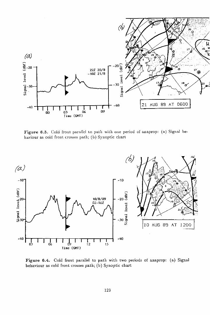
a
121 AUG 89 AT 06001
(4)
Time (GMT)
-20
> CU
-30
LO
-40
(a) CO 0
> -I
c. u-I
-10
-20
()
>
F110 AUG 89 AT 12O._j
C -30 c
U,
-4°
Figure 6.3. Cold front parallel to path with one period of anaprop: (a) Signal be-haviour as cold front crosses path; (b) Synoptic chart
(a)
Time (GMT)
Figure 6.4. Cold front parallel to path with two periods of anaprop: (a) Signal behaviour as cold front crosses path; (b) Synoptic chart
123
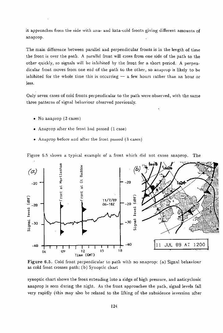
06 09 12 15 18 Time (GMT)
()
-20
I-
-20
>
U.,
-40 f ii JUL 89 AT 1200
co
-40
-20
-20
> CU
-30 Cn
Ln
it approaches from the side with ana- and kata-cold fronts giving different amounts of
anaprop.
The main difference between parallel and perpendicular fronts is in the length of time
the front is over the path. A parallel front will cross from one side of the path to the
other quickly, so signals will he inhibited by the front for a short period. A perpen-
dicular front moves from one end of the path to the other, so anaprop is likely to be
inhibited for the whole time this is occurring - a few hours rather than an hour or
less.
Only seven cases of cold fronts perpendicular to the path were observed, with the same
three patterns of signal behaviour observed previously.
. No anaprop (3 cases)
• Anaprop after the front had passed (1 case)
• Anaprop before and after the front passed (3 cases)
Figure 6.5 shows a typical example of a front which did not cause anaprop. The
Figure 6.5. Cold front perpendicular to path with no a.naprop: (a) Signal behaviour as cold front crosses path; (b) Synoptic chart
synoptic chart shows the front extending into a ridge of high pressure, and anticyclonic
anaprop is seen during the night. As the front approaches the path, signal levels fall
very rapidly (this may also be related to the lifting of the subsidence inversion after
124
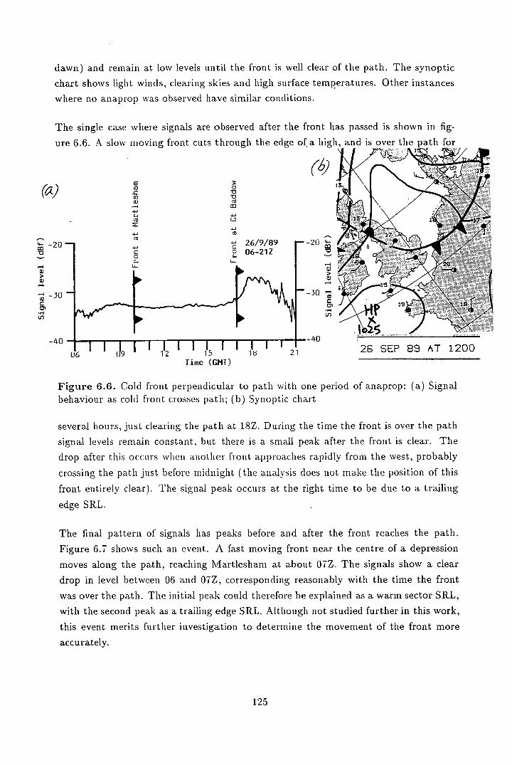
(4)
Time (GMT)
3. 0
co
LO
•0 CD
co
(a) C
(I, a)
—4
CD
Z
CD
-20
—4 a) > a) -4
-30 ca C
-20 •0
—4 a) > Q -4
-30 C
"-4 U•)
-40 -40
dawn) and remain at low levels until the front is well clear of the path. The synoptic
chart shows light winds, clearing skies and high surface temperatures. Other instances
where no anaprop was observed have similar conditions.
The single case where signals are observed after the front has passed is shown in fig-
ure 6.6. A slow moving front cuts through the edge ofia high, and is over the path for
2E SEP 89 AT 1200
Figure 6.6. Cold front perpendicular to path with one period of anaprop: (a) Signal behaviour as cold front crosses path; (b) Synoptic chart
several hours, just clearing the path at 18Z. During the time the front is over the path
signal levels remain constant, but there is a small peak after the front is clear. The
drop after this occurs when another front approaches rapidly from the west, probably
crossing the path just before midnight (the analysis does not make the position of this
front entirely clear). The signal peak occurs at the right time to be due to a trailing
edge SRL.
The final pattern of signals has peaks before and after the front reaches the path.
Figure 6.7 shows such an event. A fast moving front near the centre of a depression
moves along the path, reaching Martlesham at about 07Z. The signals show a clear
drop in level between 06 and 07Z, corresponding reasonably with the time the front
was over the path. The initial peak could therefore he explained as a warm sector SRL,
with the second peak as a trailing edge SRL. Although not studied further in this work,
this event merits further investigation to determine the movement of the front more
accurately.
125
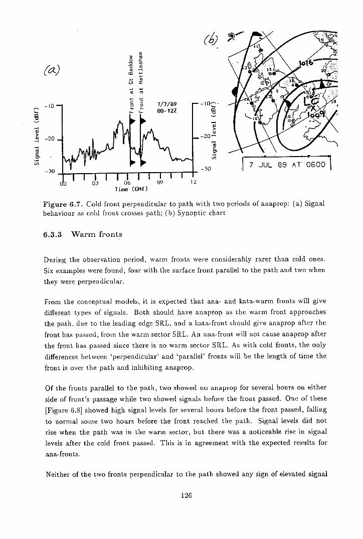
T 7 JUL89 AT oBool
C (0
or 0 0) 10 0) (0 —4
-- Co
Co (0
(a.)
__ -10
cc
—4
-20
—4 Co C
Ln
C,
-30
-1 0z . co
—I 0) > 0)
-20 —4 (0 C C,
Cl)
-30
(g)
Time (GMT)
Figure 6.7. Cold front perpendicular to path with two periods of anaprop: (a) Signal behaviour as cold front crosses path; (b) Synoptic chart
6.3.3 Warm fronts
During the observation period, warm fronts were considerably rarer than cold ones.
Six examples were found, four with the surface front parallel to the path and two when
they were perpendicular.
From the conceptual models, it is expected that ana- and kata-warm fronts will give
different types of signals. Both should have anaprop as the warm front approaches
the path, due to the leading edge SRL, and a kata-front should give anaprop after the
front has passed, from the warm sector SRL. An a.na-front will not cause anaprop after
the front has passed since there is no warm sector SRL. As with cold fronts, the only
differences between 'perpendicular' and 'parallel' fronts will be the length of time the
front is over the path and inhibiting a.naprop.
Of the fronts parallel to the path, two showed no anaprop for several hours on either
side of front's passage while two showed signals before the front passed. One of these
[Figure 6.81 showed high signal levels for several hours before the front passed, falling
to normal some two hours before the front reached the path. Signal levels did not
rise when the path was in the warm sector, but there was a noticeable rise in signal
levels after the cold front passed. This is in agreement with the expected results for
ana-fronts.
Neither of the two fronts perpendicular to the path showed any sign of elevated signal
126
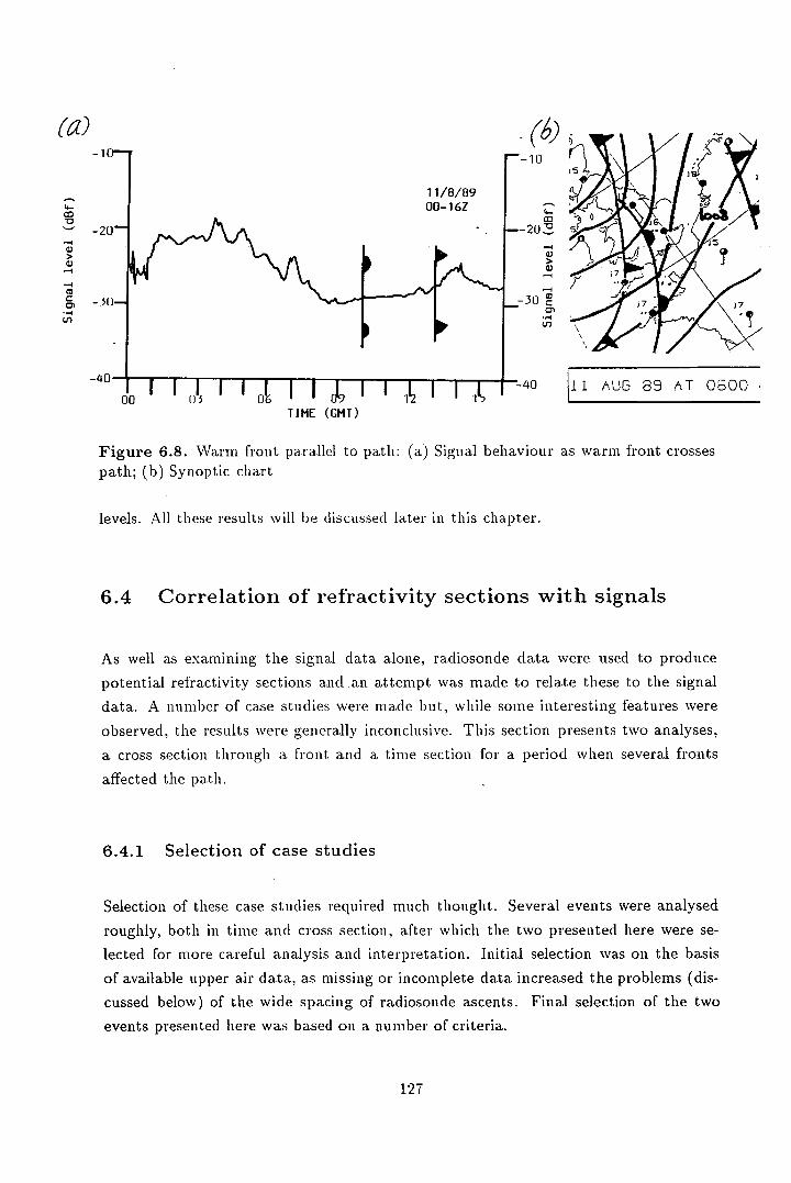
(a)
co
'- —2 '—I
> a)
—4 CO
-
U,
—4(
TIME (GMT)
)
10
cm 2O
-4 cu > W -4
—4 C
3 a C,
-4 U,
40 11 AUG 89 AT 0800
Figure 6.8. Warm front parallel to path: (a) Signal behaviour as warm front crosses path; (b) Synoptic chart
levels. All these results will be discussed later in this chapter.
6.4 Correlation of refractivity sections with signals
As well as examining the signal data alone, radiosonde data were used to produce
potential refractivity sections and an attempt was made to relate these to the signal
data. A number of case studies were made but, while some interesting features were
observed, the results were generally inconclusive. This section presents two analyses,
a cross section through a front and a time section for a period when several fronts
affected the path.
6.4.1 Selection of case studies
Selection of these case studies required much thought. Several events were analysed
roughly, both in time and cross section, after which the two presented here were se-
lected for more careful analysis and interpretation. Initial selection was on the basis
of available upper air data, as missing or incomplete data increased the problems (dis-
cussed below) of the wide spacing of radiosonde ascents. Final selection of the two
events presented here was based on a number of criteria.
127
• The cross section study was chosen from the cold fronts (since there was insuf-
ficient data. for meaningful studies of a warm or occluded front) studied earlier,
allowing comparison l)ct\VeelL the time series analysis and the refractivity section.
Analysis of a cold front also allowed comparison with the FRONTS'87 studies.
The event of 1/7/89 was eventually selected since a non-standard radiosonde as-
cent was made from Larkhill, giving extra resolution. This case study was also
part of the author's presentation at the ICAP'91 conference [Jones 19911.
• The time section studies each covered a period of 5 to 7 days with a number of
fronts passing in that time. The period 5-11/8/89 was eventually selected since
a range of frontal types (three cold fronts parallel and one perpendicular to the
signal path, together with one or two warm fronts) affected the path during that
period and there was only one missing radiosonde ascent.
Routine radiosonde ascents are made every twelve hours (00 and 12Z), from nine sites in
the British Isles. Two other sites make occasional ascents at irregular times. Since most
of the anaprop that seems to he associated with fronts lasts for considerably less than 12
hours, it is not possible to make refractivity cross sections for many cases of presumed
frontal anaprop. Similarly the space scale of about 200km between radiosonde stations
means that many features of the atmosphere are not observed because an ascent does
not pass through them.
Interpolation using a computer graphics package proved impossible since the contouring
routines did not have enough data for good interpolation. Instead contours were drawn
by hand, aided by calculated positions of the 10 K-unit isopleths on each ascent, giving
a linear interpolation. Minor isopleths were entirely hand drawn. Some obviously
incorrect data values were omitted from the interpolation scheme. Surface pressures
were not easily extracted from the tephigrams, so were ignored. This did no affect the
validity of the analysis.
6.4.2 Analysis of a refractivity cross section
The cold front of 1/7/89 was an example of anaprop before and after the front crosses
the path. The signal chart [Figure 6.9] shows these peaks. Note that the time axis has
been reversed to allow easy comparison with the refractivity structure [Figure 6.10].
As well as the position of the radiosondes, the profile also shows the approximate time
w.r.t. the passage of the surface front over the path, allowing correlation with the
signal chart. This assumes that the refractivity section moves with the front, not a
valid assumption meteorologically, but a useful approximation for this type of analysis.
128
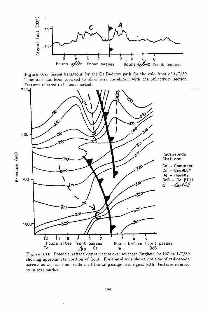
Radiosonde Stations
Ca - Camborne Cr - CraWLEY He - Hemsby DeB - De But
-h'//
:1'
E
0
1 0(
- -201 CU 0 - I
5 6 4 2 2.4 6 8 Hours front passes Hours 44#i. front passes
Figure 6.9. Signal behaviour for the Gt Baddow path for the cold front of 1/7/89. Time axis has been reversed to allow easy correlation with the refractivity section. Features referred to in text marked.
700_I ,
Hours after front passes Hours before front passes Ca / Cr He DeB
Figure 6.10. Potential refractivity structure over southern England for 12Z on 1/7/89 showing approximate position of front. Horizontal axis shows position of radiosonde ascents as well as 'time' scale w.r.t frontal passage over signal path. Features referred to in text marked
129
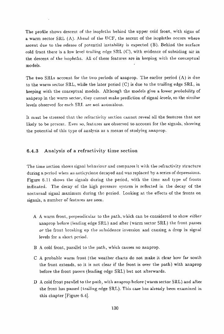
The profile shows descent of the isopleths behind the upper cold front, with signs of
a warm sector SRL (A). Ahead of the UCF, the ascent of the isopleths occurs where
ascent due to the release of potential instability is expected (B). Behind the surface
cold front there is a low level trailing edge SRL (C), with evidence of subsiding air in
the descent of the isopleths. All of these features are in keeping with the conceptual
models.
The two SRLs account for the two periods of anaprop. The earlier period (A) is due
to the warm sector SRL, while the later period (C) is due to the trailing edge SRL, in
keeping with the conceptual models. Although the models give a lower probability of
ana.prop in the warm sector, they cannot make prediction of signal levels, so the similar
levels observed for each SRL are not anomalous.
It must be stressed that the refractivity section cannot reveal all the features that are
likely to be present. Even so, features are observed to account for the signals, showing
the potential of this type of analysis as a means of studying anaprop.
6.4.3 Analysis of a refractivity time section
The time section shows signal behaviour and compares it with the refractivity structure
during a period when an anticyclone decayed and was replaced by a series of depressions.
Figure 6.11 shows the signals during the period, with the time and type of fronts
indicated. The decay of the high pressure system is reflected in the decay of the
nocturnal signal maximum during the period. Looking at the effects of the fronts on
signals, a number of features are seen.
A A warm front, perpendicular to the path, which can be considered to show either
anaprop before (leading edge SRL) and after (warm sector SRL) the front passes
or the front breaking up the subsidence inversion and causing a drop in signal
levels for a short period.
B A cold front, parallel to the path, which causes no anaprop.
C A probable warm front (the weather charts do not make it clear how far south
the front extends, so it is not clear if the front is over the path) with anaprop
before the front passes (leading edge SRL) but not afterwards.
D A cold front parallel to the path, with anaprop before (warm sector SRL) and after
the front has passed (trailing edge SRL). This case has already been examined in
this chapter [Figure 6.4].
130
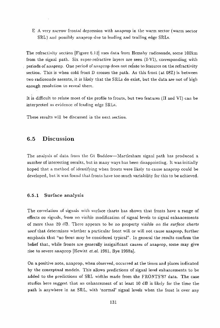
E A very narrow frontal depression with anaprop in the warm sector (warm sector
SRL) and possibly anaprop due to leading and trailing edge SRLs.
The refractivity section [Figure 6.121 uses data from Hemshy radiosonde, some 100km
from the signal path. Six super-refractive layers are seen (1-VI), corresponding with
periods of anaprop. One period of anaprop does not relate to features on the refractivity
section. This is when cold front D crosses the path. As this front (at 08Z) is between
two radiosonde ascents, it is likely that the SRLs do exist, but the data are not of high
enough resolution to reveal them.
It is difficult to relate most of the profile to fronts, but two features (II and VI) can be
interpreted as evidence of leading edge SRLs.
These results will be discussed in the next section.
6.5 Discussion
The analysis of data from the Gt Bacidow—Martlesham signal path has produced a
number of interesting results, but in many ways has been disappointing. It was initially
hoped that a method of identifying when fronts were likely to cause anaprop could be
developed, but it was found that fronts have too much variability for this to be achieved.
6.5.1 Surface analysis
The correlation of signals with surface charts has shown that fronts have a range of
effects on signals, from no visible modification of signal levels to signal enhancements
of more than 20 dB. There appears to be no property visible on the surface charts
used that determines whether a particular front will or will not cause anaprop, further
emphasis that "no front may be considered typical". In general the results confirm the
belief that, while fronts are generally insignificant causes of anaprop, some may give
rise to severe anaprop [Hewitt et.al. 1981, Bye 1988a].
On a positive note, anaprop, when observed, occurred at the times and places indicated
by the conceptual models. This allows predictions of signal level enhancements to be
added to the predictions of SRL widths made from the FR.ONTS'87 data. The case
studies here suggest that an enhancement of at least 10 dB is likely for the time the
path is anywhere in an SilL, with 'normal' signal levels when the front is over any
131
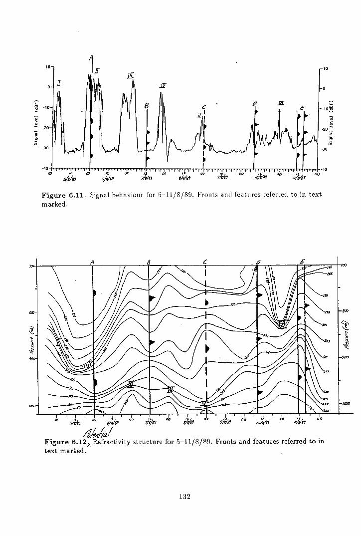
93
>
C
U,
>
C
U,
ltv
lox
Figure 6.11. Signal behaviour for 5-11/8/89. Fronts and features referred to in text marked.
A C 0 ___ -700
70
/ \\ se -Ia
I I I I I I •
- 7/(/8 9/c/iT
Figure 6.12 Refractivity structure for 5-11/8/89. Fronts and features referred to in text marked.
\
900
132
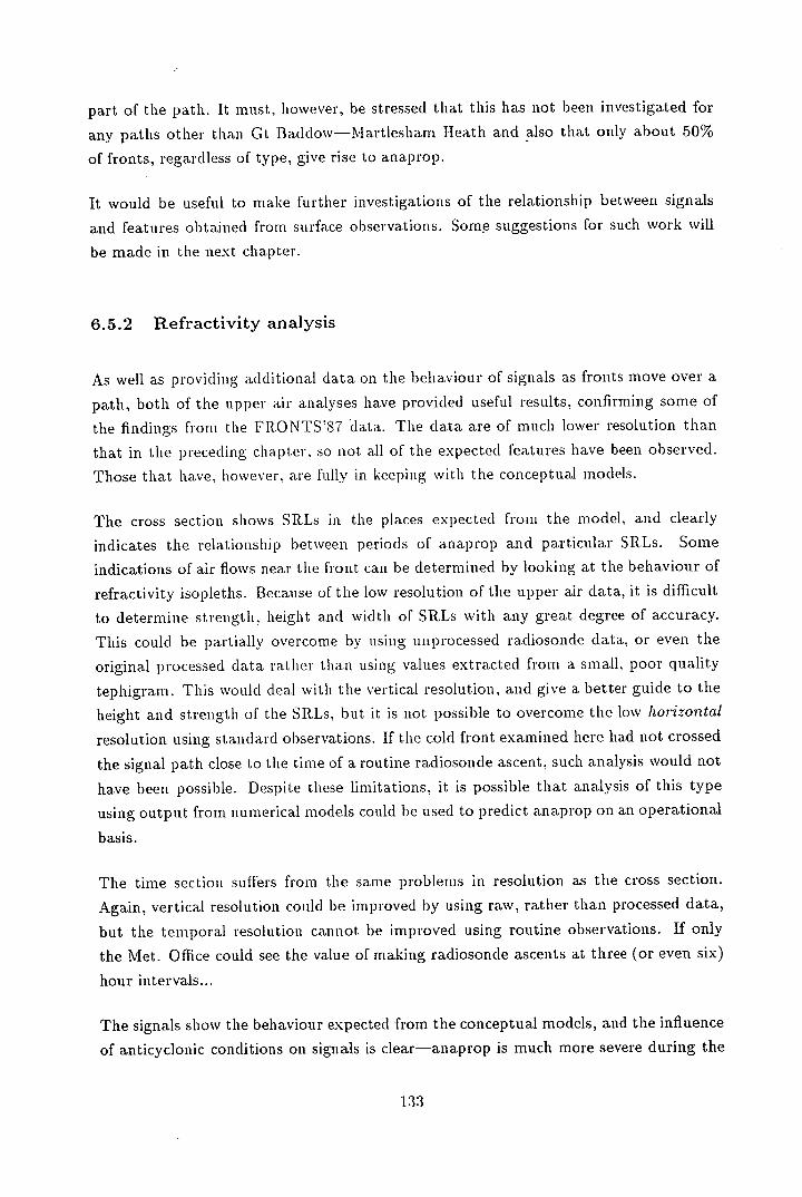
part of the path. It must, however, he stressed that this has not been investigated for
any paths other than Gt Bacldow—Martlesham Heath and also that only about 50%
of fronts, regardless of type, give rise to anaprop.
It would be useful to make further investigations of the relationship between signals
and features obtained from surface observations. Som.e suggestions for such work will
be made in the next chapter.
6.5.2 Refractivity analysis
As well as providing additional data on the behaviour of signals as fronts move over a
path, both of the upper air analyses have provided useful results, confirming some of
the findings from the FRONTS'87 data. The data are of much lower resolution than
that in the preceding chapter, so not all of the expected features have been observed.
Those that have, however, are fully in keeping with the conceptual models.
The cross section shows SItLs in the places expected from the model, and clearly
indicates the relationship between periods of anaprop and particular SRLs. Some
indications of air flows near the front can be determined by looking at the behaviour of
refractivity isopleths. Because of the low resolution of the upper air data, it is difficult
to determine strength, height and width of SRLs with any great degree of accuracy.
This could be partially overcome by using unprocessed radiosonde data, or even the
original processed data rather than using values extracted from a small, p°°' quality
tephigram. This would deal with the vertical resolution, and give a better guide to the
height and strength of the SRLs, but it is not possible to overcome the low horizontal
resolution using standard observations. If the cold front examined here had not crossed
the signal path close to the time of a routine radiosonde ascent, such analysis would not
have been possible. Despite these limitations, it is possible that analysis of this type
using output from numerical models could he used to predict anaprop on an operational
basis.
The time section suffers from the same problems in resolution as the cross section.
Again, vertical resolution could be improved by using raw, rather than processed data,
but the temporal resolution cannot be improved using routine observations. If only
the Met. Office could see the value of making radiosonde ascents at three (or even six)
hour intervals...
The signals show the behaviour expected from the conceptual models, and the influence
of anticyclonic conditions on signals is clear—anaprop is much more severe during the
133

first three days of the analysis. than at the end, when the weather had become cyclonic.
The refractivity section shows that almost all the anaprop can be ascribed to different
SRLs, but it is less easy to see which of the Sills are frontal in origin. This is (again)
a result of the low resolution of the data. Despite the negative tone of this discussion,
the analysis of the Ct Baddow data has provided much qualitative evidence in support
of the conceptual models. The determination of the variability of frontal anaprop has
also been useful, and plOvi(ICS many hints as to where further study may be fruitful.
134

Chapter 7
Conclusions
To bring this work to a close, this chapter provides a final overview of the thesis. It
begins with a chapter by chapter summary of the main findings, bringing the various
sections into a coherent whole. This is followed by a number of suggestions for further
research and finally by a personal evaluation of the whole project.
7.1 Summary of findings
Excluding the literature survey, which, althou ,0ti vital to the research, does not con-
tribute anything to the results, each chapter of this thesis contributes important results.
Most of the findings are linked by the conceptual models [Chapter 4], which provide a
framework for interpreting observational results.
Chapter 3 examines the effects of different weather conditions as causes of anaprop. The
results can be summarised in the significance ratios, the amount of anaprop caused by
a given weather type as a ratio of the amount of time that type occurs for [Figures 7.1
& 7.2]. These, and other results, confirm the expectation that anticyclones are the
most important cause of anaprop [Bye 1988a], with fronts as a relatively insignificant
source of interference propagation, statistically speaking. This does not stop some
fronts causing very severe anaprop [e.g. Hewitt et.al. 1981].
This work is one of only two to study the effects of different weather conditions on
anaprop, and uses a far more detailed classification scheme and greater range of signal
paths than the other work [Spillard 1991]. Results for each weather type have been used
135
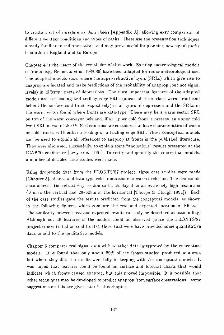
to create a. set of interference data .:heets [Appendix A], allowing easy comparison of
different weather conditions and types of paths. These use the presentation techniques
already familiar to radio scientists, and may prove useful for planning new signal paths
in southern England and to Europe.
Chapter 4 is the heart of the remainder of this work. Existing meteorological models
of fronts [e.g. Bennetts et.ai. 1988,89] have been adapted for radio-meteorological use.
The adapted models show where the super-refractive layers (SRLs) which give rise to
anaprop are located and make predictions of the probability of anaprop (but not signal
levels) in different parts of depressions. The most important features of the adapted
models are the leading and trailing edge SRLs (ahead of the surface warm front and
behind the surface cold front respectively) in all types of depression and the SRLs in
the warm sector found where fronts are kata-type. There may be a warm sector SRL
on top of the Wlll conveyor belt and, if an upper cold front is present, an upper cold
front SRL ahead of the UCF. Occlusions are considered to have characteristics of warm
or cold fronts, with either a leading or a trailing edge SRL. These conceptual models
can be used to explain all references to anaprop at fronts in the published literature.
They were also used, successfully, to explain some"anomalous" results presented at the
ICAP'91 conference [Levy et.al. 1991]. To verify and quantify the conceptual models,
a number of detailed case studies were made.
Using dropsonde data from the FRONTS'87 project, three case studies were made
[Chapter 5], of ana- and ka.ta-type cold fronts and of a warm occlusion. The dropsonde
data allowed the refractivity section to he displayed to an extremely high resolution
(lOrn in the vertical and 20-60km in the horizontal [Thorpe & Clough 1991]). Each
of the case studies gave the results predicted from the conceptual models, as shown
in the following figures, which compare the real and expected location of SRLs.
The similarity between real and expected results can only he described as astounding!
Although not all features of the models could be observed (since the FRONTS'87
project concentrated on cold fronts), those that were have provided some quantitative
data to add to the qualitative models.
Chapter 6 compares real signal data with weather data interpreted by the conceptual
models. It is found that only about 50% of the fronts studied produced anaprop,
but where they did, the results were fully in keeping with the conceptual models. It
was hoped that features could be found on surface and forecast charts that would
indicate which fronts caused anaprop, but this proved impossible. It is possible that
other techniques may be developed to predict ana.prop from surface observations—some
suggestions on this are given later in this chapter.
137
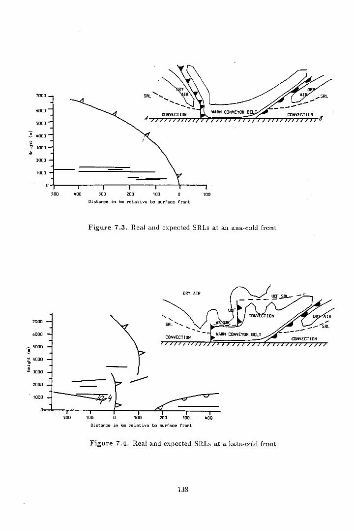
7000
6000
5000
4000
3000
2000
1000
•0
500
SRL
CONVECTION - WARM CONVEYOR BEL CONVECTION
JfJIJJJIfJJ If '/1 IffJ I I JfIf JJI JJJII
I I 1 I 400 300 200 100 0 100
Distance in km relative to surface front
Figure 7.3. Real and expected SRLs at an ana-cold front
DRY AIR
( - -
UCF
7000
6000
- 5000
4000
-1 .1 =3000
2000
1000
SRI
\ 9 Z~DRLI R SRL CONVECTION
WARN OEY0R BELT CONVECTION
200 100 0 100 200 300 400
Distance in km relative to surface front
Figure 7.4. Real and expected SRLs at a kata-cold front
138
DRY \AIR\
TRAILING S
EDGE SRI
ULD WARN FRONT FRONT ALOFT ALOFT
DRY Al
SRL I WARN COLD AIR
6000
I 4000
3000
(LIFTED COOL AIR
0 200 1I0 ii io
Distance in km relative to leading edge of cold front aloft
Figure 7.5. Real and expected STtLs in a warm occlusion
Looking at refractivity sections obtained from routine radiosonde ascents provided fur-
ther evidence to support the conceptual models. Anaprop on signal charts could easily
be related to SRLs on refractivity sections and, in some cases, the refractivity struc-
ture could be related to the conceptual models. This was not always possible, since the
resolution of the data was poor in both time and space. (Compare 500-1000m in the
vertical and 200-300km in the horizontal with the resolution of the FRONTS'87 data.)
All the studies of fronts showed how variable they can be, and how difficult it is to draw
general conclusions from a limited number of case studies. Through the conceptual
models, however, it is now possible to make useful predictions of the extent and, to a
certain degree, of the severity of frontal anaprop. These predictions may be of use to
BTL when operating their telecommunications network.
7.2 Further work
As with any piece of work, this thesis has raised questions as quickly as it has answered
them. This section considers some of the unresolved problems that have been found
during the work. Since this research was sponsored by industry, further work will
depend on the need industry perceives for it. From the author's viewpoint, there are
several areas that provide scope for further work.
139
• The statistics of a.naprop presented here show significant differences between dif -
ferent weather conditions but in some cases the analysis is hampered by lack of
data.. As with any statistical analysis, adding further data. will improve the ac-
curacy. Such data are available from the COST 210 project and it would not be
a difficult task to acid at least two more years to the two years already studied.
• The statistical analysis is confined to signal paths in the UK-Netherlands region,
so it is not known how valid the conclusions are for other parts of the world.
Radio- climatological maps could possibly give some indication of similar regions,
but it would be useful to produce IDS portfolios for other regions where good
signal data are available.
• The conceptual models of fronts used by meteorologists are continually changing
in the light of new research, so it would be useful to update the models presented
here on a regula.r basis.
• The Meteorological Office are planning to follow up the FR.ONTS'87 project with
further detailed studies of fronts. These could provide further verification of the
conceptual models presented here, and perhaps extend the verification to more
types of fronts. It would he particularly useful to set up signal paths in the area
of any new project, allowing a very detailed look at the relationships between
signals and the structure of fronts. Such a project would be a, major undertaking
and would require a. great deal of co-operation between the Met Office and the
researchers involved.
• Although the examination of surface charts and signal data from the Gt Baddow
path did not reveal any features that determined whether a front would produce
anaprop, it is possible that such features could be found. By examining hourly
or three-hourly surface observations, and by applying a. scheme similar to that
used by BTL to predict radiation nights [L.ochtie 1985], it might be possible to
identify which fronts produce a.na.prop.
• Many further case studies similar to those on the Great Baddow path could be
made. It would be useful to compare the effects of fronts in the UK and on similar
paths in Europe. It would also be useful to re-analyse some of the events to take
more account of the speed of the front. This would allow better comparison of
'similar' events. It would also be useful to try to understand why some fronts
cause anaprop while others don't appear to. This could be a consequence of the
direction the front approaches the signalpath from or due to upper air features
of the fronts.
• The effects of the sea breeze on ana.prop over coastal regions appears in need of
further investigation. Of particular importance is the relationship between the
140
sea breeze and offshore advection. On the downwind coastline, the sea breeze
could be cotisiclered as an extension of the advection duct onshore as fax inland
as the terrain allows, but what happens on the upwind coast? If advection is
weak, the sea breeze may bring moist air inland, giving the possibility of a.naprop
in the coastal zone, but how does this affect the formation of the advection duct?
If advection is stronger, the inland penetration of the sea breeze must be limited
to some extent but again the formation of the advection duct is bound to he
affected. These, and related, questions could possibly be answered through the
use of a relatively simple two-dimensional model of the transport of moisture and
heat between land and sea. Such a: piece of research should he a very fruitful field
for further study.
• A potentially interesting field of study is the energy spectrum of a.na.prop. Me-
teorological studies [Stull 1988 1)32] show that energy is mainly concentrated in
the synoptic scale (periods between 10 and 100 hours) and in the turbulent scale
(periods less than 0.1 hour), with an 'energy gap' between them. It would be
interesting to perform a spectral analysis of high resolution signal data and cor-
relate it with the energy spectra of different meteorological variables, particularly
those of pressure, temperature and moisture, that control the refractivity.
7.3 Evaluation
This brief, and personal, evaluation of the whole research is a welcome opportunity for
me to switch from the third to the first person.
When I began this work, the goals were to determine the cause, effects and scale of
frontal ana.prop, and to put it into place in the wider field of radio-meteorology. With
the aid of some judicious shifting of the goal-posts, all this has been achieved. As well
as these explicit goals. I felt from the beginning of the project that an unwritten, but
very important, goal was to increase the links between meteorology and radio-science,
but whether this has been achieved, only time will tell. The need for such links was,
for me, highlighted by reactions to my contribution to the ICAP'91 conference, where
I was asked many questions about conceptual models of fronts and how they could
be applied to different aspects of radio propagation. That such knowledge should be
familiar to meteorologists for more than a decade but unfamiliar to the majority of
radio-meteorologists seems to me to be indicative of the need for more links between
the disciplines. Meteorologists, too, may be able to learn from the wealth of data
collected by radio scientists on the detailed structure of the lower atmosphere.
141

I would like, again, to thank everyone who has helped me during the course of this
work. A full list would be too long to print, but you all know who you are! Special
thanks, though, to all my friends, both old and new, who have stood by me over the
last few years. Without your support, none of this would have seen the light of day.
Thanks, also, to the legions of previous workers in meteorology and radio-science whose
researches I have drawn on. As Sir Isaac Newton so truly said,
"If I have seen further, it is because I have stood on the shoulders of
giants."
142

Appendix A
Interference data sheets
The following material is a. copy of the full portfolio of interference data sheets produced
during this work.
Interference data sheets
Interference data sheets (IDSs) Provide a summary of signal behaviour under different
weather conditions. A total of 24 different weather types have been defined and for
classification purposes paths have been divided into 'Dutch' (running from Martlesham
Heath (in East Anglia) to the Netherlands) and 'UK' (running from Martlesham Heath
to other point on the UK mainland) types. This classification is discussed further in
this thesis. Each IDS has the same format:
A cumulative distribution showing summer, winter and whole year signals for
the weather type, as well as the total for all weather types. Summer refers to
the half-year from May to October, while winter refers to the half year running
from November to April. The percentages are the amount of signals at a given
level relative to the total amount of signals observed. The CD indicates seasonal
differences as well as the importance of signals produced by each weather type.
A chart showing the behaviour of signals in the course of a year at three different
levels (45, 30 and 15 dB below the free space level). The chart shows the per-
centage of the total years signals for that weather type and level received during
each month. This again shows seasonal differences, giving more detail than the
143
CD.
A chart, in the same format as the annual chart, showing the diurnal behaviour
of signals. The percentages are of the total years signals for the weather type and
level received during each hour. This chart can give indications of the anaprop
mechanisms at work, particularly for anticyclonic weather types, using conceptual
models such as Bye [1988].
A synoptic chart from the Daily Weather Report [HMSO 1986-71 showing a typical
example of the weather type. This chart, by comparison with forecast charts,
allows some predictions of anaprop to he made.
A written summary, including: The frequency of the weather type as a percentage
of the entire summer and winter ; The significance ratio for summer and winter.
This is the percentage of total signals recorded for the weather type divided by
the percentage of the time for which that the type occurs. An SR. of 1 indicates
average amounts of signals for the weather type. SRs greater than 1 denote above
average amounts of signals, indicating the weather type is a significant cause of
anaprop while SRs less than 1 signify below average amounts of signals, indicating
the weather type inhibits a.naprop.
A summary of the main features of the charts and an indication of the mechanisms
responsible for the anaprop. These mechanisms are based on work by BTL [Bye
1988] and by the author.
When using the IDSs, it is worth noting the following points. Firstly, weather systems
can be very variable, so particular events may well give results quite different from the
statistical summaries shown here. Secondly, some weather types do not have enough
data to make the analysis meaningful. These cases, typically giving data for one or two
signal producing events, are indicated on the sheets. One weather type, AF6 on Dutch
paths, has no recorded cases. For completeness, a blank IDS is given for this type.
144
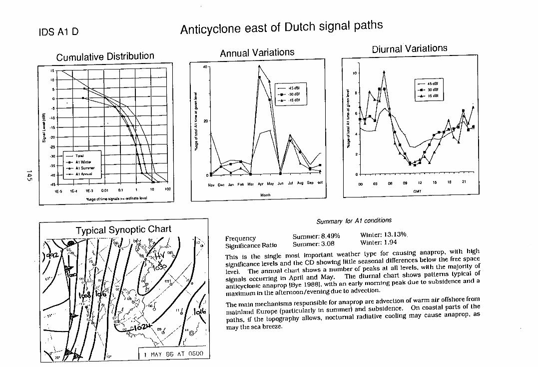
IDS Al D Anticyclone east of Dutch signal paths
Cumulative Distribution
g Total Al Wintar
u Al 'iII%I I..
A_......I I.-.+;,r'i'
J1
Typical Synoptic Chart
Or
03
" J t,o2 \09 /_,tl / \\ ,. / 1
1 °' 1A 86 AT 0600
Summary for Al conditions
Frequency Summer: 8.49% Winter: 13.13%.
Significance Ratio Summer: 3.08 Winter: 1.94
This Is the single most important weather type for causing anaprop, with high significance levels and the CD showing little seasonal differences below the free space level. The annual chart shows a number of peaks at all levels, with the majority of signals occurring in April and May. The diurnal chart shows patterns typical of anticyclonic anaprop (Bye 19881, with an early morning peak due to subsidence and a maximum In the afternoon/evening due to advection.
The main mechanisms responsible for anaprop are advection of warm air offshore from mainland Europe (particularly in summer) and subsidence. On coastal parts of the paths, if the topography allows, nocturnal radiative cooling may cause anaprop, as
may the sea breeze.
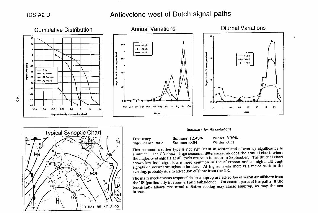
IDS A2D
Anticyclone west of Dutch signal paths
Cumulative Distribution
MMMMMMM MMMMMMM
A2Wntm
Sum uI-Iu'-I I1I
Anni iI \Iritirnc flhiirnI Viritinns
Typical Synoptic Chart
08: jO
1016 - / •\1016(
03
09
10
'1
\ 7
07
t ' 4-K 1009
-° ?. •
- 70 , . MAY 86 AT 2400
Summary for A2 conditions
Frequency Summer: 12.45% Winter: 8.32% Significance Ratio Summer: 0.94 Winter: 0.11
This common weather type is not significant In winter and of average significance in summer. The CD shows large seasonal differences, as does the annual chart, where the majority of signals at all levels are seen to occur in September. The diurnal chart shows low level signals are more common in the afternoon and at night, although signals do occur throughout the day. At higher levels there is a major peak in the evening, probably due to advection offshore from the UK.
The main mechanisms responsible for anaprop are advection of warm air offshore from the UK (particularly in summer) and subsidence. On coastal parts of the paths, if the topography allows, nocturnal radiative cooling may cause anaprop, as may the sea breeze.
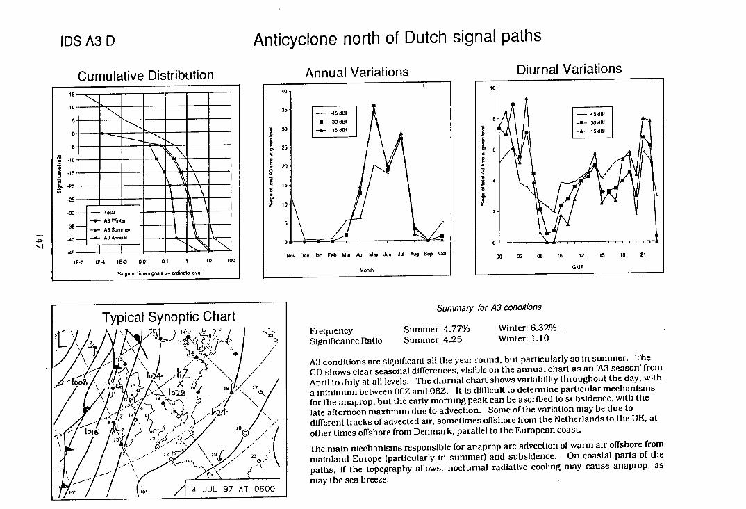
IDS A3D Anticyclone north of Dutch signal paths
Cumulative Distribution
Tot
at
A3 S uIIIII\U
Aririi iI \/rkitirtnQ flhmrrl
Typical Synoptic Chart L~j J4
12 9 is
JA
14 1~d 1016
oo
(;o. /[A JUL 87 AT 0600
Summary for A3 conditions
Frequency Summer: 4.77% Winter: 6.32%
Significance Ratio Summer: 4.25 Winter: 1.10
A3 conditions are significant all the year round, but particularly so in summer. The CD shows clear seasonal differences, visible on the annual chart as an 'A3 season' from April to July at all levels. '['he diurnal chart shows varlal)ility throughout the day, with a minimum between OGZ and 08Z. It is difficult to determine particular mechanisms for the anaprop, but the early morning peak can be ascribed to subsidence, with the late afternoon maximum due to advection. Some of the variation may be due to different tracks of advected air, sometimes offshore from the Netherlands to the UK, at other times offshore from Denmark, parallel to the European coast.
The main mechanisms responsible for anaprop are advection of warm air offshore from mainland Europe (particularly In summer) and subsidence. On coastal parts of the paths, if the topography allows, nocturnal radiative cooling may cause anaprop, as may the sea breeze.
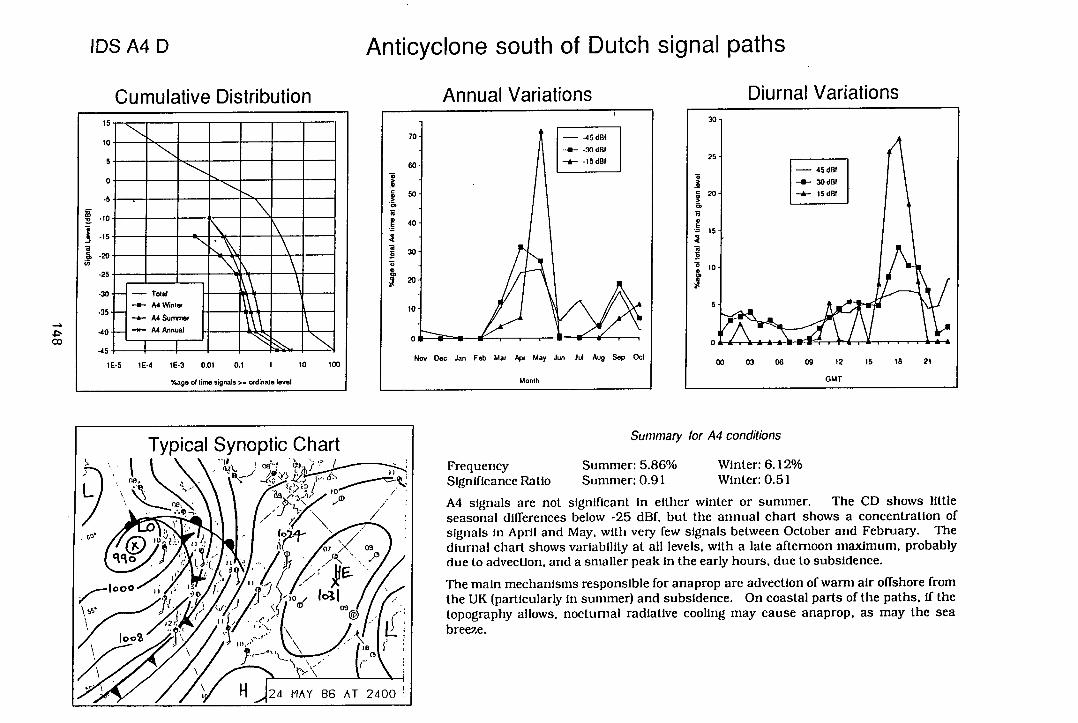
IDS A4D
Anticyclone south of Dutch signal paths
Cumulative Distribution
Arini iI Iricifrne flhiirnI IrtirnQ
Total
A4 Winter
A4 Summer —a
A4 Annual
cc
Summary for A4 conditions
Frequency Summer: 5.86% Winter: 6.12% Significance Ratio Summer: 0.91 Winter: 0.51
A4 signals are not significant in either winter or summer. The CD shows little seasonal differences below -25 dBf, but the annual chart shows a concentration of signals in April and May, with very few signals between October and February. The diurnal chart shows variability at all levels, with a late afternoon maximum, probably due to advection, and a smaller peak in the early hours, due to subsidence.
The main mechanisms responsible for anaprop are advection of warm air offshore from the UK (particularly in summer) and subsidence. On coastal parts of the paths, if the topography allows, nocturnal radiative cooling may cause anaprop, as may the sea breeze.
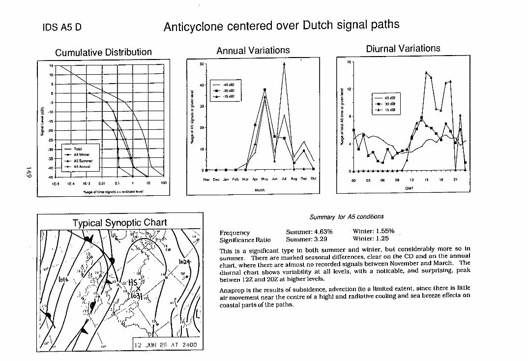
A.......-.I i- :. ....-.-.I
IDS A5D Anticyclone centered over Dutch signal paths
'.0
Cumulative Distribution
W11111111111 =M mm MM MW MM MM MIM. mm Elk M mm M mm 1111 WE__
AS Winim
I,,IuiI-I--I all • __
Typical Synoptic Chart
•! I .. \ \-Y
o•I
I v I Ile I I
/ 10(6 -, VCHS
12 JUN 8F, AT 2400
Summary for A5 conditions
Frequency Summer: 4.63% Winter: 1.55% Significance Ratio Summer: 3.29 Winter: 1.25
This is a significant type in both summer and winter, but considerably more so in summer. There are marked seasonal differences, clear on the CD and on the annual chart, where there are almost no recorded signals between November and March. The diurnal chart shows variability at all levels, with a noticable, and surprising, peak betwen 12Z and 20Z at higher levels.
Anaprop is the results of subsidence. advection (to a limited extent, since there is little air movement near the centre of a high) and radiative cooling and sea breeze effects on coastal parts of the paths.
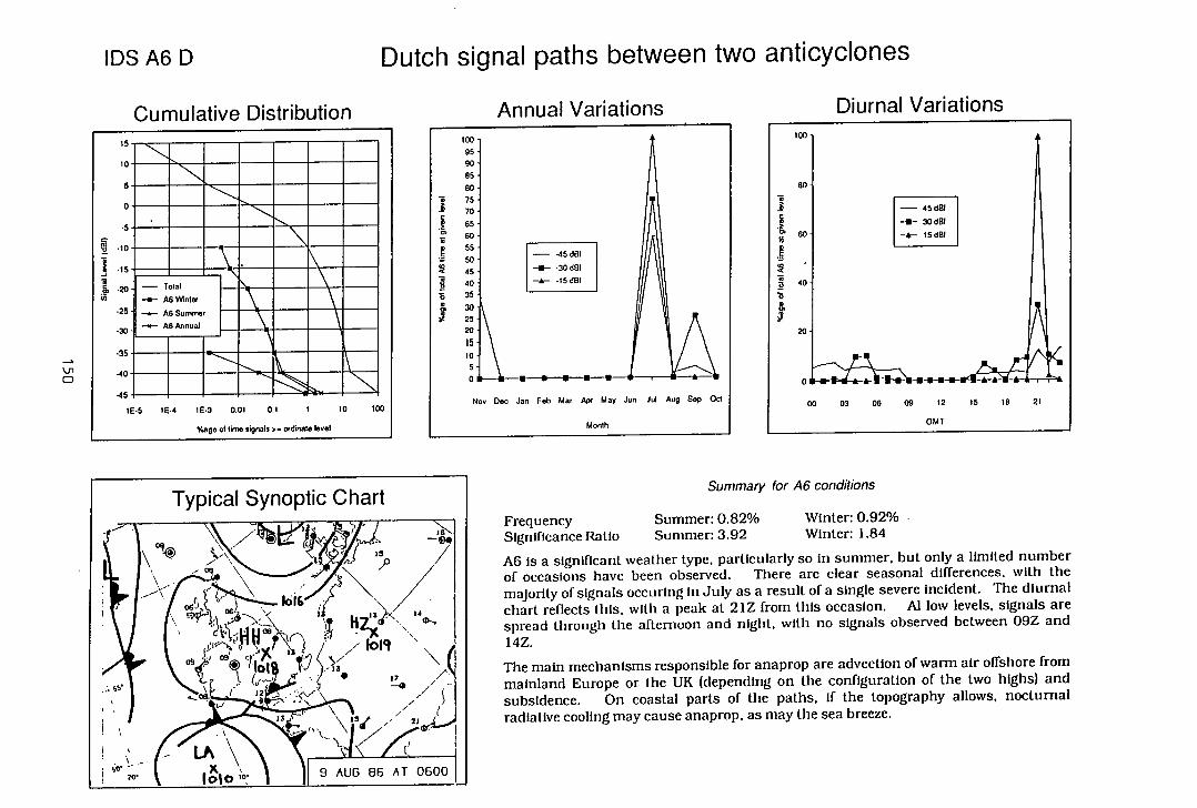
IDS A6D Dutch signal paths between two anticyclones
Cumulative Distribution AnniiI Viritirns fliiirnI Variations
M
!!#ffl —a— A6 Wmfer ii i•i
A6 nuad
Typical Synoptic Chart
C )c /\ /
I \) f ht4ci '1 114
/ 1014 ° ¶?NZ
32
33 is 4e 21
10
Summary for A6 conditions
Frequency Summer: 0.82% Winter: 0.92% Significance Ratio Summer: 3.92 Winter: 1.84
A6 is a significant weather type, particularly so in summer, but only a limited number of occasions have been observed. There are clear seasonal differences, with the majority of signals occuring in July as a result of a single severe Incident. The diurnal chart reflects this, with a peak at 21Z from this occasion. Al low levels, signals are spread through the afternoon and night, with no signals observed between 09Z and 14Z.
The main mechanisms responsible for anaprop are advection of warm air offshore from mainland Europe or the UK (depending on the configuration of the two highs) and subsidence. On coastal parts of the paths, if the topography allows, nocturnal radiative cooling may cause anaprop, as may the sea breeze.
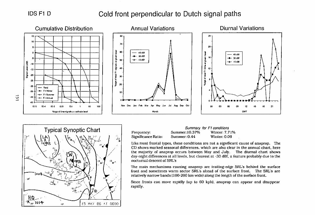
IDS F1 D
Cold front perpendicular to Dutch signal paths
Cumulative Distribution
Annual Variations
Diurnal Variations
-'
SI-_I FA
Typical Synoptic Synoptic Chart
12
n >Y
100%.
k
.........
/ o@_ ,
---. -.--------,I ,J .
. lolj . 15 MAY 86 AT 0600
Summary for Fl conditions Frequency: Summer: 10.37% Winter: 7.71% Significance Ratio: Summer: 0.44 Winter: 0.09
Like most frontal types, these conditions are not a significant cause of anaprop. The CD shows marked seasonal differences, which are also clear in the annual chart, here the majority of anaprop occurs between May and July. The diurnal chart shows day-night differences at all levels, but clearest at -30 dBf, a feature probably due to the nocturnal descent of SRL's
The main mechanisms causing anaprop are trailing-edge SRL's behind the surface front and sometimes warm sector SRL's ahead of the surface front. The SRL's are relatively narrow bands (100-200 km wide) along the length of the surface front.
Since fronts can move rapidly (up to 60 kph), anaprop can appear and disappear rapidly.
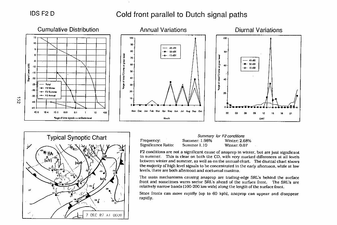
IDS F2D
Cold front parallel to Dutch signal paths
Cumulative Distribution
Anni iil \Iritir%nc
flh.rnI
2 Summer
I Typical Synoptic Chart
-00
102 W14 2
-OJ 03
10
02
EC8?FOQ(
Summary for F2 conditions Frequency: Summer: 1.98% Winter: 2.68% Significance Ratio: Summer 1.10 Winter: 0.07
F2 conditions are not a significant cause of anaprop in winter, but are just significant in summer. This is clear on both the CD, with very marked differences at all levels between winter and summer, as well as on the annual chart. The diurnal chart shows the majority of high level signals to be concentrated in the early afternoon, while at low levels, there are both afternoon and nocturnal maxima.
The main mechanisms causing anaprop are trailing-edge SRL's behind the surface front and sometimes warm sector SRL's ahead of the surface front. The SRL's are relatively narrow bands (100-200 km wide) along the length of the surface front.
Since fronts can move rapidly (up to 60 kph), anaprop can appear and disappear rapidly.
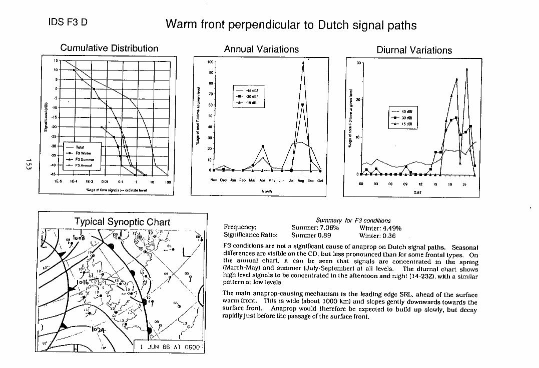
IDS F3D
Warm front perpendicular to Dutch signal paths
Cumulative Distribution
Anni iI
fliiirnI \/rkifirtno
- ¼)'
kin MM MEN
Total
F3 Winte, MV M.111111111111 F3 Su r F3 Ann at 11=11111011
Typical Synoptic Chart
12
09 3
10. 1 JUN 86ITI
Summary for F3 conditions Frequency: Summer: 7.06% Winter: 4.49% Significance Ratio: Summer 0.89 Winter: 0.36
F3 conditions are not a significant cause of anaprop on Dutch signal paths. Seasonal differences are visible on the CD. but less pronounced than for some frontal types. On the annual chart, It can be seen that signals are concentrated In the spring (March-May) and summer (July-September) at all levels. The diurnal chart shows high level signals to be concentrated in the afternoon and night (14-23Z. with a similar pattern at low levels.
The main anaprop-causing mechanism Is the leading edge SRI., ahead of the surface warm front. This is wide (about 1000 km) and slopes gently downwards towards the surface front. Anaprop would therefore be expected to build up slowly, but decay rapidlyjust before the passage of the surface front.
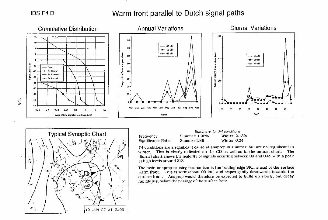
IDS F4D
Warm front parallel to Dutch signal paths
Cumulative Distribution
Annual Variations
Diurnal Variations
IIIl
IMIMM
4. MMIMM
Typical Synoptic Chart '\\
'4
Cq
09 ,
"
~\
\\__,/\
14
87 AT 2400
Summary for F4 conditions Frequency: Summer: 1.98% Winter: 2.13% Significance Ratio: Summer 1.86 Winter: 0.24
F4 conditions are a significant cause of anaprop in summer, but are not significant in winter. This is clearly indicated on the CD as well as In the annual chart. The diurnal chart shows the majority of signals occuring between 09 and OOZ, with a peak at high levels around 21Z.
The main anaprop-causing mechanism is the leading edge SRL, ahead of the surface warm front. This is wide (about 00 km) and slopes gently downwards towards the surface front. Anaprop would therefore be expected to build up slowly, but decay rapidlyjust before the passage of the surface front.
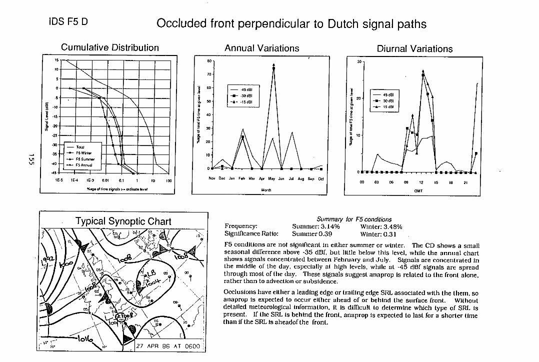
IDS F5 D Occluded front perpendicular to Dutch signal paths
Cumulative Distribution
AnniiI Vritinn
flit irnI Iritir'nc
MMMMMM - MMMMMMM MMMMMMM
Total
IWinter IE--- i F5 Annual
Typical Synoptic Chart 67
, X -,
0z\
CA
JJ N'Z f X
_\_- 1 ''/' ,' •
rbo 20, N. 'r 1 27 APR 86 AT 0600 1
Summary for F5 conditions Frequency: Summer: 3.14% Winter: 3.48% Significance Ratio: Summer 0.39 Winter: 0.31
F5 conditions are not significant in either summer or winter. The CD shows a small seasonal difference above -35 dBf, but little below this level, while the annual chart shows signals concentrated between February and July. Signals are concentrated In the middle of the day, especially at high levels, while at -45 dBf signals are spread through most of the day. These signals suggest anaprop Is related to the front alone, rather than to advection or subsidence.
Occlusions have either a leading edge or trailing edge SRL associated with the them, so anaprop Is expected to occur either ahead of or behind the surface front. Without detailed meteorological information, It Is difficult to determine which type of SRL Is present. If the SRI. is behind the front, anaprop Is expected to last for a shorter time than if the SRL is aheadof the front.
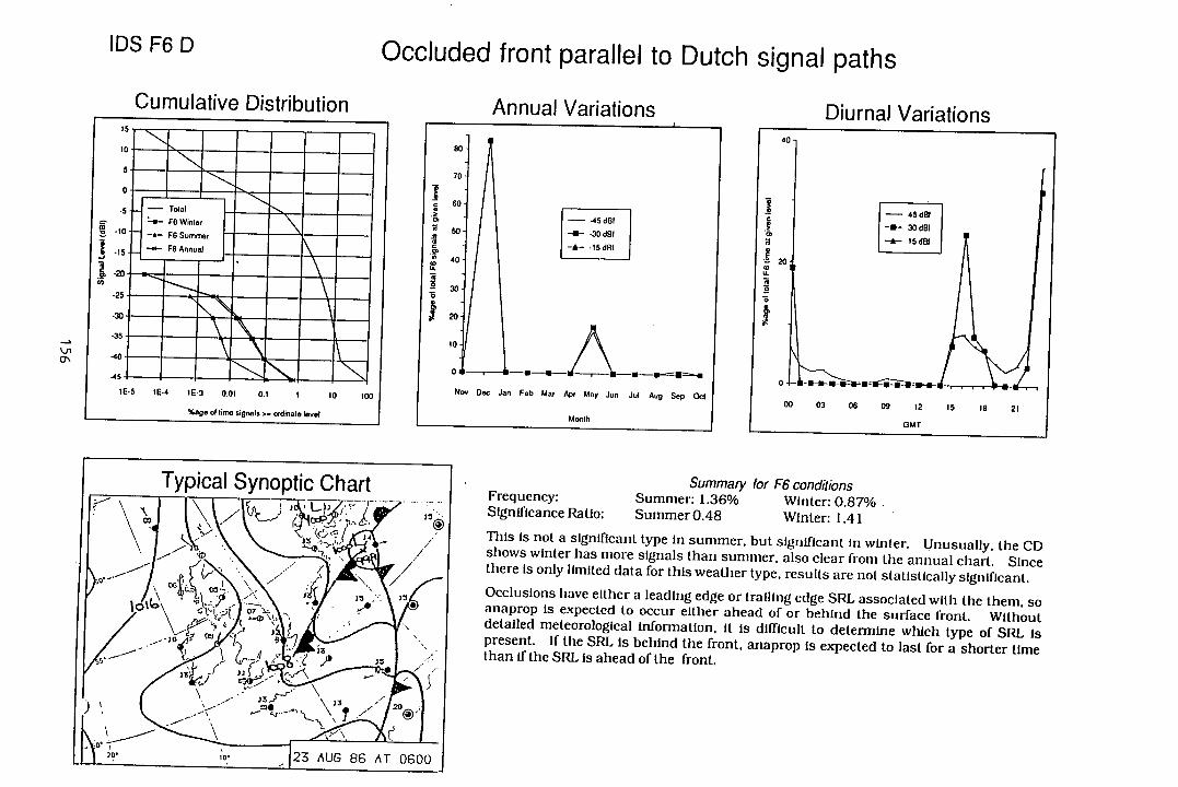
IDS F6 D Occluded front parallel to Dutch signal paths
Ci imi iIfiic flicfrihi ifrr AnniiI /arkfirtno fliijrniI Thritirno
-. Ln
Summary for F6 conditions Frequency: Summer: 1.36% Winter: 0.87% Significance Ratio: Summer 0.48 Winter: 1.41
This is not a significant type In summer, but significant in winter. Unusually, the CD shows winter has more signals than summer, also clear from the annual chart. Since there is only limited data for this weather type, results are not statistically significant.
Occlusions have either a leading edge or trailing edge SRL associated with the them, so anaprop is expected to occur either ahead of or behind the surface front. Without detailed meteorological information, it is difficult to determine which type of SRL is present. If the SRL Is behind the front, anaprop is expected to last for a shorter time than if the SRL is ahead of the front.
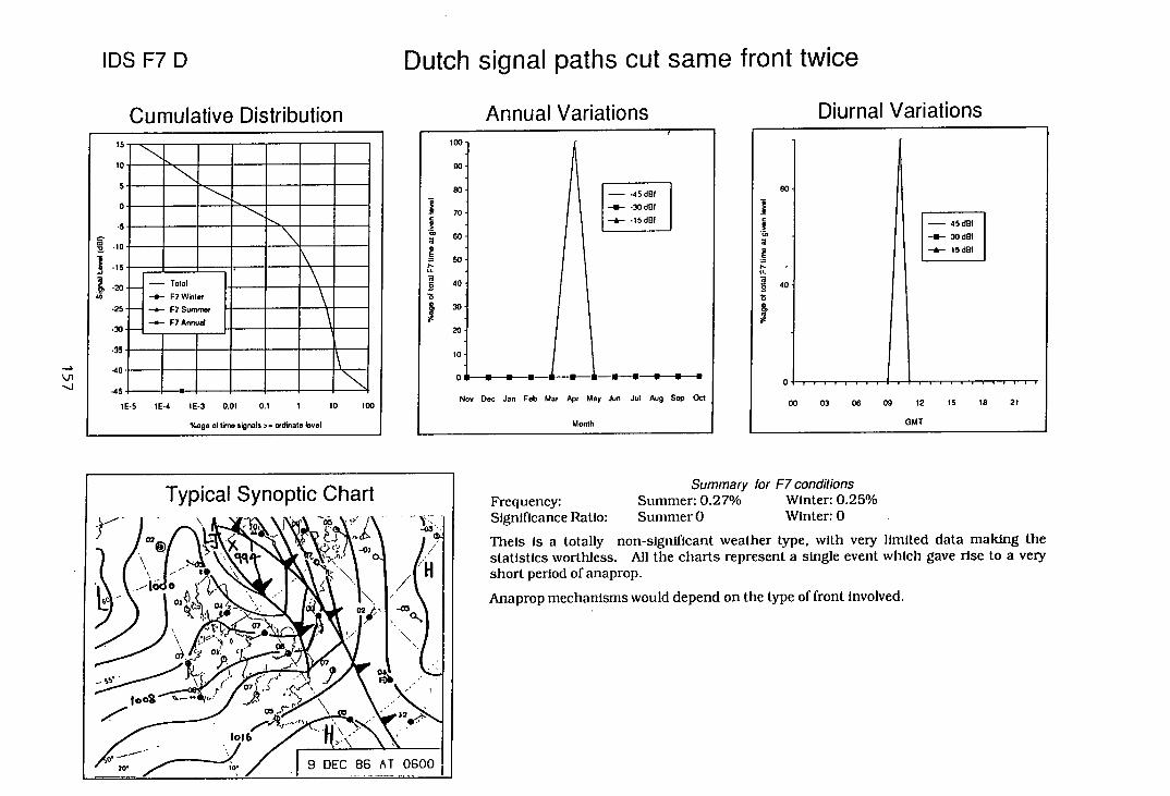
IDS F7D
Dutch signal paths cut same front twice
Cumulative Distribution
A rrii iI \/rktirnc
n;i,rI /ri!1+irflO
—a
977
F7 Annual
MMOMMMMM MMMMMMkM
Typical Synoptic Chart 03
02 M
02
07
02
05
) )°
4
32
- '°'I
/-./j 9 DEC 86ii±Iooi
Summary for F? conditions Frequency: Summer: 0.27% Winter: 0.25% Significance Ratio: Summer 0 Winter: 0
Theis is a totally non-significant weather type, with very limited data making the statistics worthless. All the charts represent a single event which gave rise to a very short period of anaprop.
Anaprop mechanisms would depend on the type of front involved.
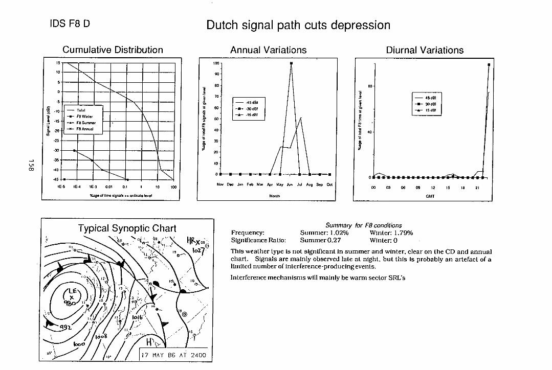
------ 1
mmmmmmm
mmmmmmm
L..
'2
\t / ir
7-
IDS F8D
Dutch signal path cuts depression
Cumulative Distribution
AnniiI Vriitinns
Diurnal Variations
Typical Synoptic Chart "'
12 , ID
7' fL 111.41 s.:f O2 1 3 I i IO' I I ij
" II/) fuLl loi
..v' /fi00% / 1000/
I I- fio' / / 117 MAY AT 2400
Summary for F8 conditions
Th is weather type is not significant In summer and winter, clear on the CD and annual chart. Signals are mainly observed late at night, but this is probably an artefact of a limited number of interference-producing events.
Frequency: Summer: 1.02% Winter: 1.79% Significance Ratio: SunmierO.27 Winter: 0
Interference mechanisms will mainly be warm sector SRL's
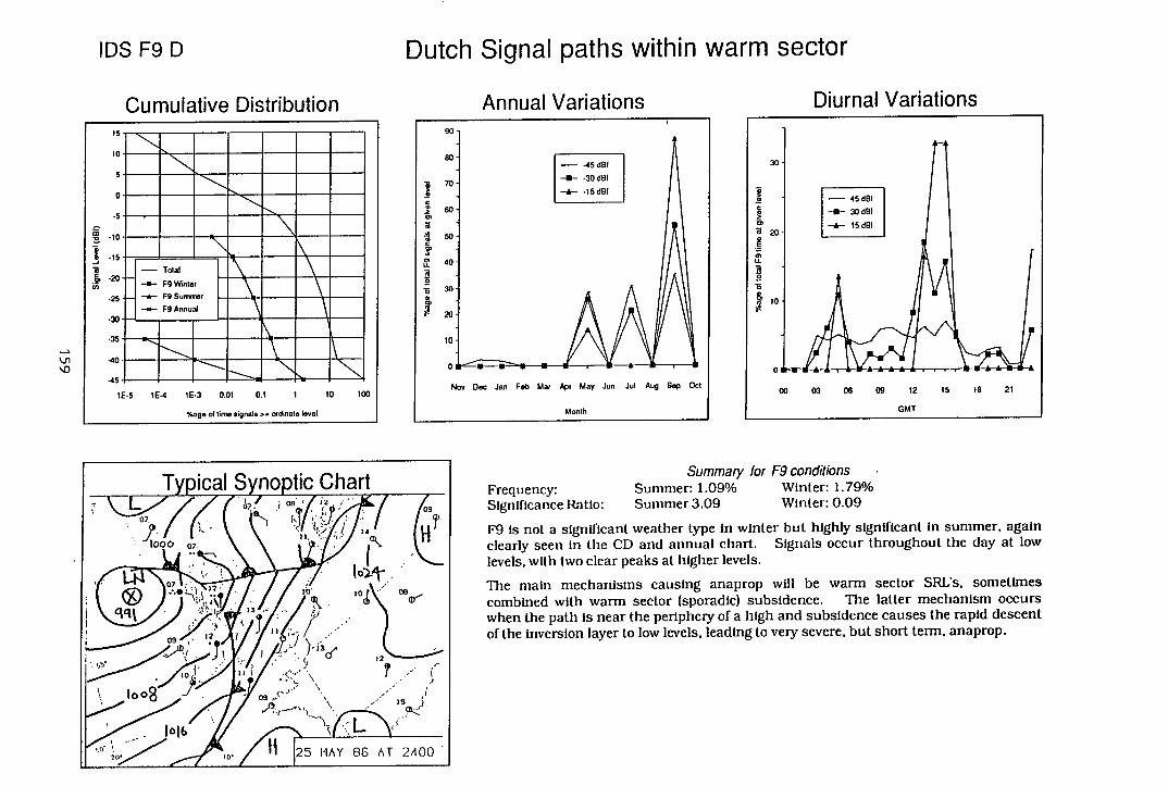
noptic Chart 09
JA
IQ'/
09
11 25 HAY 86 AT 2400
TvDical
Jf ( \ 1000 07.
0
32
V qq J. I
09
\ Ioo 7
1 0 16
/
IDS F9D
Dutch Signal paths within warm sector
Cumulative Distribution Anniiil Vritions
fli,irnI Vritions
'0
MMMMMM MMMMMMM MMMMMMM
JIL FgAnnuad
Summary for F9 conditions Frequency: Summer: 1.09% Winter: 1.79% Significance Ratio: Summer 3.09 Winter: 0.09
F9 is not a significant weather type in winter but highly significant in summer, again clearly seen in the CD and annual chart. Signals occur throughout the day at low levels, with two clear peaks at higher levels.
The main mechanisms causing anaprop will be warm sector SRL's, sometimes combined with warm sector (sporadic) subsidence. The latter mechanism occurs when the path is near the periphery of a high and subsidence causes the rapid descent of the Inversion layer to low levels, leading to very severe, but short term, anaprop.
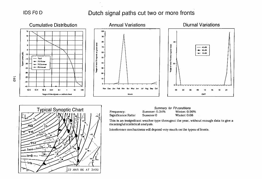
IDS FOD
Dutch signal paths cut two or more fronts
Cumulative Distribution
Anni iiI Viricitinnc. fliiirniI Vritinnc
—a 0\
-I
111177 =Otal
0— FO Winter
FO SU-1
Typical Synoptic Chart
03 1
J 3 A4f/oz
qq 01
oj/
1 10
oL
MAR 86 AT 2400
Summary for FO conditions Frequency: Summer: 0.34% Winter: 0.96% Significance Ratio: Summer 0 Winter: 0.08
This is an inslgnlfcant weather type througout the year. without enough data to give a meaningful statistical analysis.
Interference mechanisms will depend very much on the types of fronts.
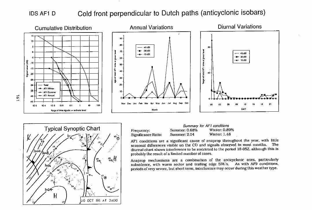
IDS AR D Cold front perpendicular to Dutch paths (anticyclonic isobars)
Cumulative Distribution
Annual Variations
Diurnal Variations
0'
-.j'flhI1-I'---I AF1 Summer
Typical Synoptic Chart
/17°Aoe8,: JI1I ....... 03 01
(T\ /i' / #' .................' I°
. I I
102+
7
10 OCT 86 AT 2400
Summary for AF1 conditions Frequency: Summer: 0.68% Winter: 0.89% Significance Ratio: Summer: 2.04 Winter: 1.48
AF1 conditions are a significant cause of anaprop throughout the year, with little seasonal differences visible on the CD and signals observed in most months. The diurnal chart shows interference to be restricted to the period 18-05Z. although this Is probably the result of a limited number of cases.
Anaprop mechanisms are a combination of the anticyclonic ones, particularly subsidence, with warm sector and trailing edge SRL's. As with AF9 conditions, periods of very severe, but short term, interference may occur during this weather type.
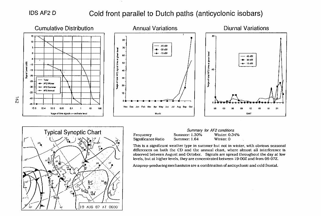
IDS AF2 D Cold front parallel to Dutch paths (anticyclonic isobars)
Cumulative Distribution
A rru ,.iI Irifr%nc' ri;, er r .-I
—a ON
a— 02Wnter
Typical Synoptic Chart
17
1%
c4, 14
10
7fl\. Hs
19 AUG 87 AT 0800
Summary for AF2 conditions Frequency Summer: 1.30% Winter: 0.34% Significance Ratio Summer: 1.64 Winter: 0
This is a significant weather type in summer but not in winter, with obvious seasonal differences on both the CD and the annual chart, where almost all interference Is observed between August and October. Signals are spread throughout the day at low levels, but at higher levels, they are concentrated between 19-OOZ and from 06-07Z.
Anaprop-producing mechanisms are a combination of anticyclonic and cold frontal. .,o.__-_ \I-A"07
IJ 37
.i\ 7 2?'
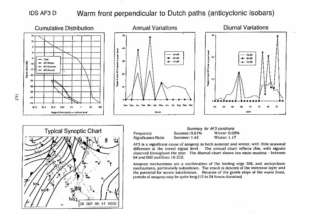
IDS AF3 D Warm front perpendicular to Dutch paths (anticyclonic isobars)
Cumulative Distribution
Anni iI Vnrinfinnc fliiirnil Irktir'nc
0'
MMMMMMM MMMMMMM
TotW
I All Into(
MMIMMMMIM
Summary for AF3 conditions Frequency Summer: 0.61% Winter: 0.69% Significance Ratio Summer: 1.43 Winter: 1.17
AM Is a significant cause of anaprop in both summer and winter, with little seasonal difference at the lowest signal level. The annual chart reflects this, with signals observed throughout the year. The diurnal chart shows two main maxima - between 04 and 09Z and from 16-21Z.
Anaprop mechanisms are a combination of the leading edge SRL and anticyclonic mechanisms, particularly subsidence. The result is descent of the inversion layer and the potential for severe interference. Because of the gentle slope of the warm front. periods of anaprop may be quite long (12 to 24 hours duration)
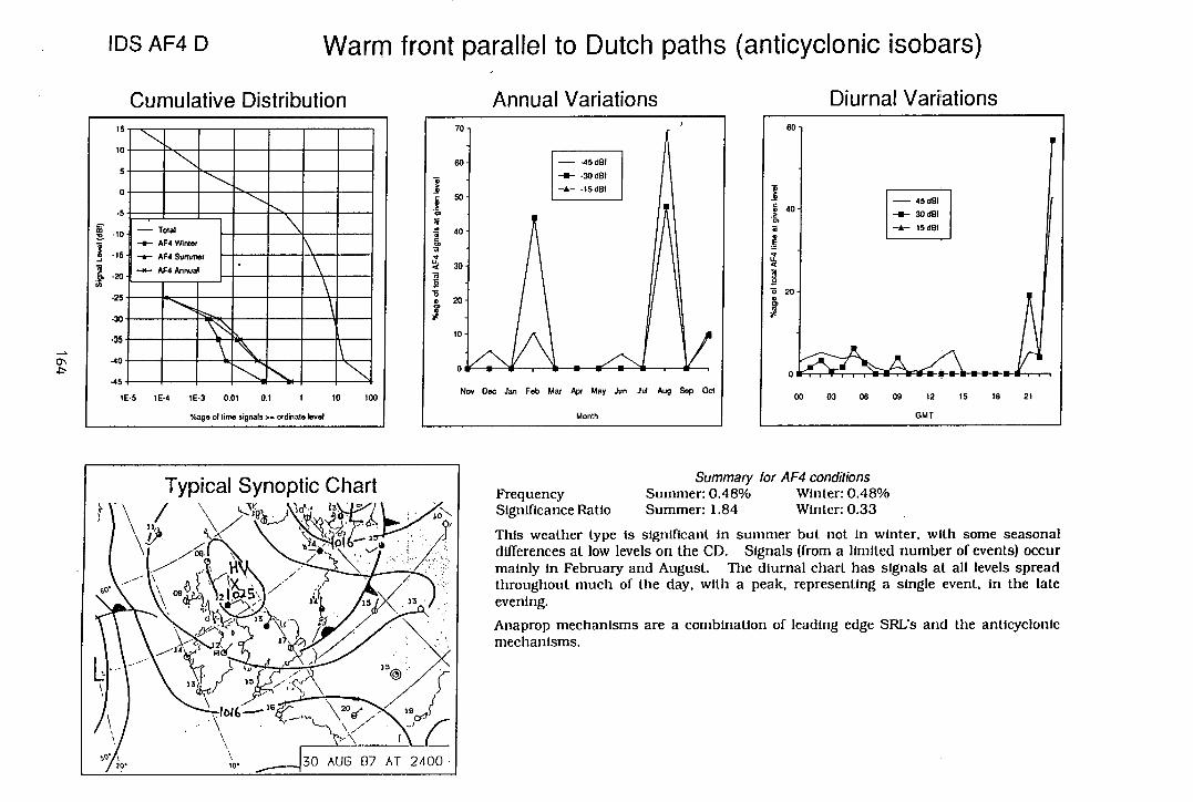
IDS AF4 D Warm front parallel to Dutch paths (anticyclonic isobars)
Cumulative Distribution Annual Variations Diurnal Variations
crs
MMMMMMM
MMMMMMM •1 I1iri.I I
AR Annual 1MM111§M • _______
--- -
-----
Typical Synoptic Chart
C3 33
15 lot
. '-430 AUG 87 AT 2400
Summary for AF4 conditions Frequency Summer: 0.48% Winter: 0.48% Significance Ratio Summer: 1.84 Winter: 0.33
This weather type is significant In summer but not in winter, with some seasonal differences at low levels on the CD. Signals (from a limited number of events) occur mainly in February and August. The diurnal chart has signals at all levels spread throughout much of the day. with a peak, representing a single event, in the late evening.
Anaprop mechanisms are a combination of leading edge SRL's and the anticyclonic mechanisms.
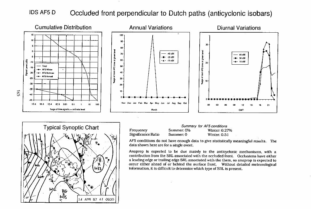
0"
MMMMMMMM MMMMMMMM MMMMMMMM MMMMMMMM MMMMMM
AFS now
MMMMMMMM
MMMM MM
IDS AF5 D Occluded front perpendicular to Dutch paths (anticyclonic isobars)
........ .I4:. . r:...4..:L. .4...... A ._. ....i i_.._,._ - ,_ - -
Typical Synoptic Chart
00
07
10 "(' I
J ]4 APR 87 AT 0600 -
Summary for AF5 conditions Frequency Summer: 0% Winter: 0.27% Significance Ratio Summer: 0 Winter: 0.51
AF5 conditions do not have enough data to give statistically meaningful results. The data shown here are for a single event.
Anaprop Is expected to be due mainly to the anticyclonic mechanisms, with a contribution from the SRL associated with the occluded front. Occlusions have either a leading edge or trailing edge SRI. associated with the them, so anaprop is expected to occur either ahead of or behind the surface front. Without detailed meteorological Information, It is difficult to determine which type of SRL is present.
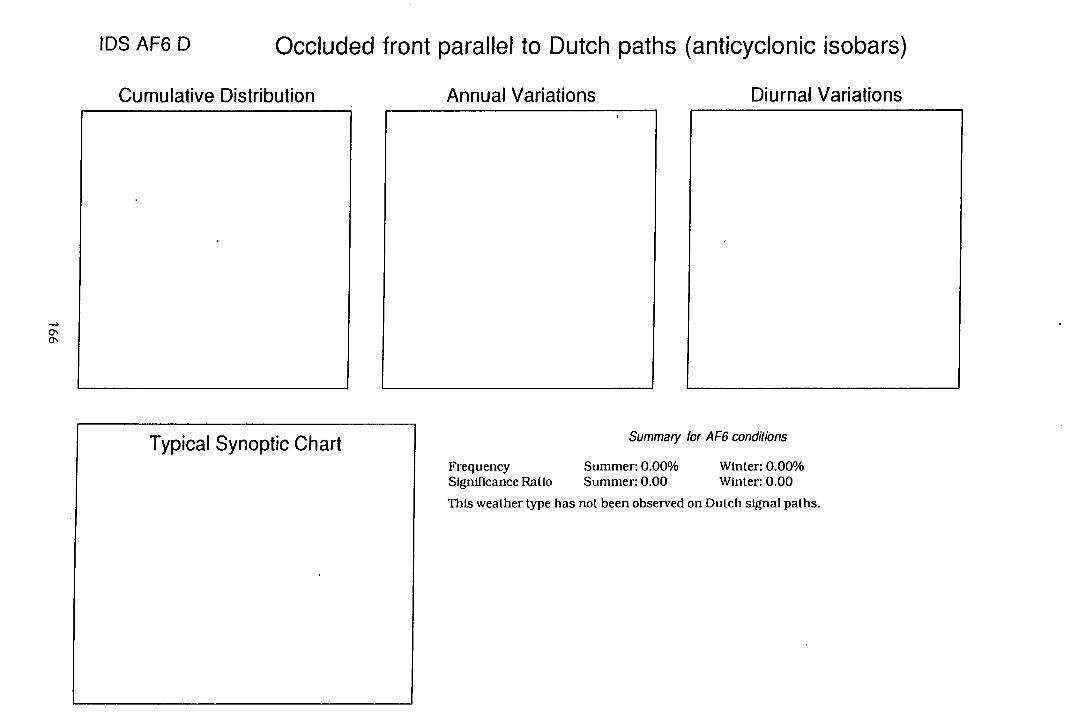
IDS AF6 D Occluded front parallel to Dutch paths (anticyclonic isobars)
Cumulative Distribution Annual Variations Diurnal Variations
0 .
Typical Synoptic Chart Summary for AF6 conditions
Frequency Summer: 0.00% Winter: 0.00% Significance Ratio Summer: 0.00 Winter: 0.00
This weather type has not been observed on Dutch signal paths.
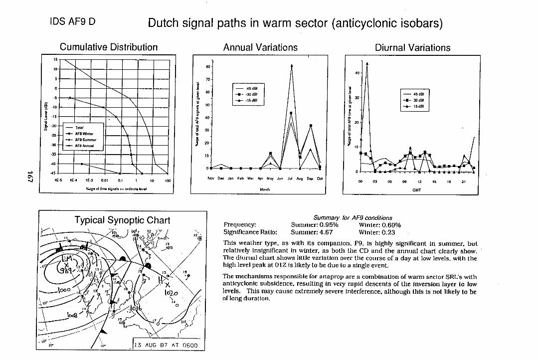
IDS AF9 D Dutch signal paths in warm sector (anticyclonic isobars)
Cumulative Distribution
Anni ,I \/rfirnc
fliirnI
0\ '.4
MMMMMM MMMMMMM MMMMMMM
MEMMMMM
UMIJL. AF
S-7 I'MMUM'M
Typical Synoptic Chart 126
IG
._1000 'ji ( / to2o \/
#2 ?<c \
0. I13 AUG 87 AT 0600
Summary for AF9 conditions Frequency: Summer: 0.95% Winter: 0.69% Significance Ratio: Summer: 4.67 Winter: 0.23
This weather type, as with its companion, F9, Is highly significant in summer, but relatively insignificant In winter, as both the CD and the annual chart clearly show. The diurnal chart shows little variation over the course of a day at low levels, with the high level peak at 01Z is likely to be due to a single event.
The mechanisms responsible for anaprop are a combination of warm sector SRL's with anticyclonic subsidence, resulting In very rapid descents of the inversion layer to low levels. This may cause extremely severe interference, although this Is not likely to be of long duration.
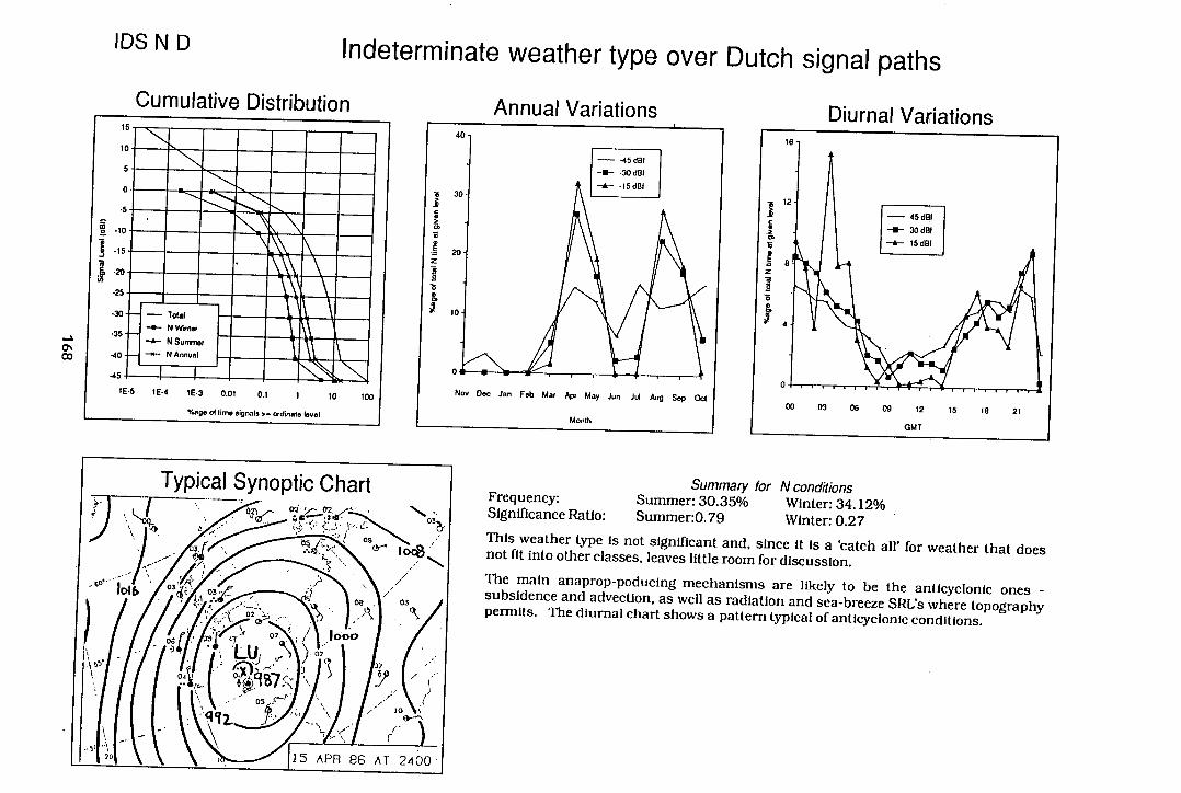
Cumultiv flitrihi ifirn Annual V2riutinn Diurnal Varitinn
0\ CO
IDS N 0 Indeterminate weather type over Dutch signal paths
Typical Synoptic Chart 00
as
as 03
15 APR 86 AT 2400
Summary for N Conditions Frequency: Summer: 30.35% Winter: 34.12% Significance Ratio: Summer:0.79 Winter: 0.27
This weather type is not significant and, since it is a 'catch all' for weather that does not fit into other classes, leaves little room for discussion.
The main anaprop-poducing mechanisms are likely to be the anticyclonic ones - subsidence and advection, as well as radiation and sea-breeze SRL's where topography permits. The diurnal chart shows a pattern typical of anticyclonic conditions.
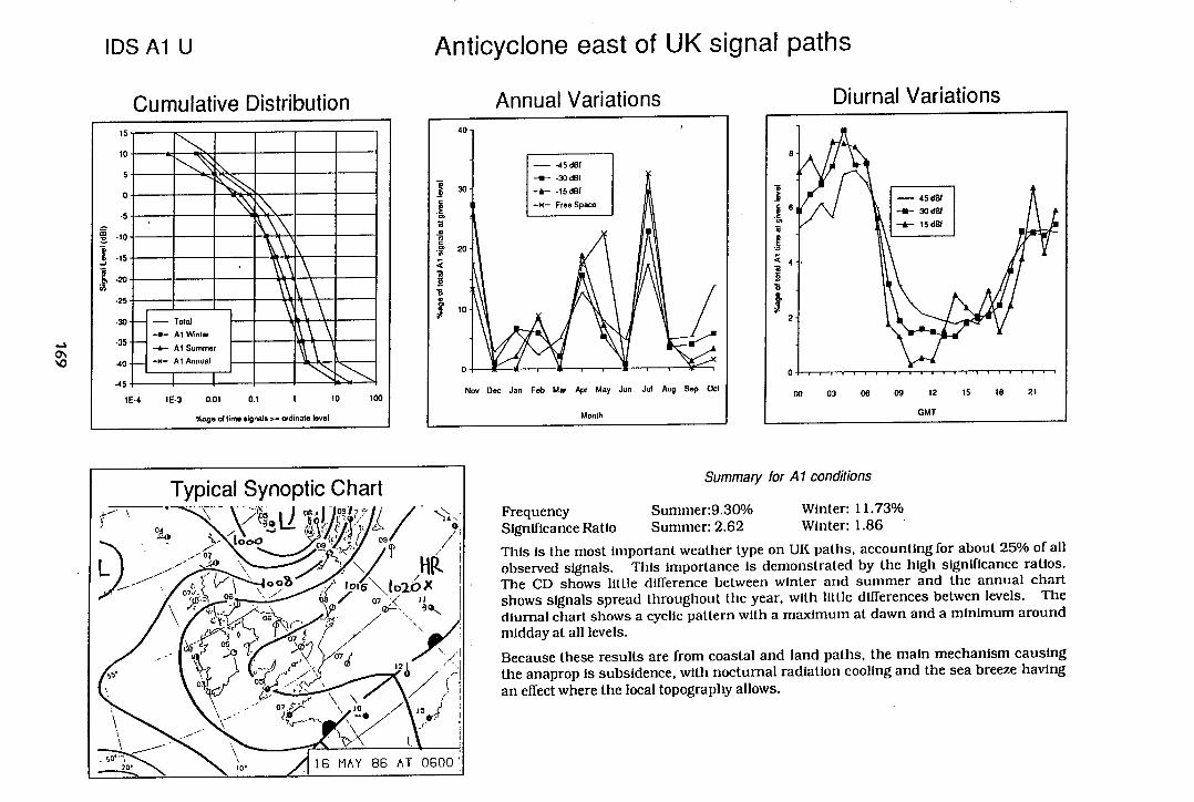
IDS Al U
Anticyclone east of UK signal paths
ON '0
Cumulative Distribution
_i- 11 WIN I
_________ I _____
______ I
--\!I
Al I'.J.__ •___.
Annual Variations Diurnal Variations
Typical Synoptic Chart
07
107 V2 x>10 X
07 4
Summary for Al conditions
Frequency Summer:9.30% Winter: 11.73% Significance Ratio Summer: 2.62 Winter: 1.86
This is the most important weather type on UK paths, accounting for about 25% of all observed signals. This importance is demonstrated by the high significance ratios. The CD shows little difference between winter and summer and the annual chart shows signals spread throughout the year. with little differences betwen levels. The diurnal chart shows a cyclic pattern with a maximum at dawn and a minimum around midday at all levels.
Because these results are from coastal and land paths, the main mechanism causing the anaprop is subsidence, with nocturnal radiation cooling and the sea breeze having an effect where the local topography allows.
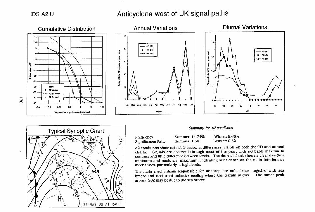
Cumulative Distribution
•i_ I
____ ____I III __I
___I _____
Total •4 I
A rrlI i.I /iriitirtna r..rr.iI
IDS A2U
Anticyclone west of UK signal paths
Typical Synoptic Chart
t7\ xI 7
I
W
07
1009
N. / MAY 86 AT 2400
Summary for A2 conditions
Frequency Summer: 14.74% Winter: 9.66% Significance Ratio Summer: 1.56 Winter: 0.52
A2 conditions show noticable seasonal differences, visible on both the CD and annual charts. Signals are observed through most of the year, with noticable maxima in summer and little difference between levels. The diurnal chart shows a clear day-time minimum and nocturnal maximum, indicating subsidence as the main interference mechanism, particularly at high levels.
The main mechanisms responsible for anaprop are subsidence, together with sea breeze and nocturnal radiative cooling where the terrain allows. The minor peak around 20Z may be due to the sea breeze.
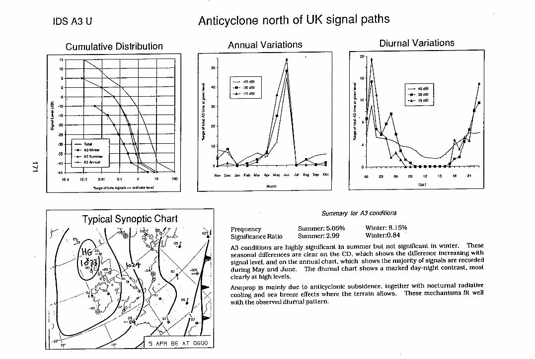
Cumulative Distribution
liii I III vtI___I
16SA a A3 Surnme'
A3 Annual
ONES
IDS A3U
Anticyclone north of UK signal paths
Summary for A3 conditions
10
Frequency Summer: 5.05% Winter: 8.15% Significance Ratio Summer: 2.99 Winter:0.84
A3 conditions are highly significant In summer but not significant in winter. These seasonal differences are clear on the CD, which shows the difference increasing with signal level, and on the annual chart, which shows the majority of signals are recorded during May and June. The diurnal chart shows a marked day-night contrast, most clearly at high levels.
Anaprop is mainly due to anticyclonic subsidence, together with nocturnal radiative cooling and sea breeze effects where the terrain allows. These mechanisms fit well with the observed diurnal pattern.
Typical Synoptic Chart
o
I - 0
.--.-.
-00
o• _
t o'X
QP 03,
/
5 APR 85 AT 0600
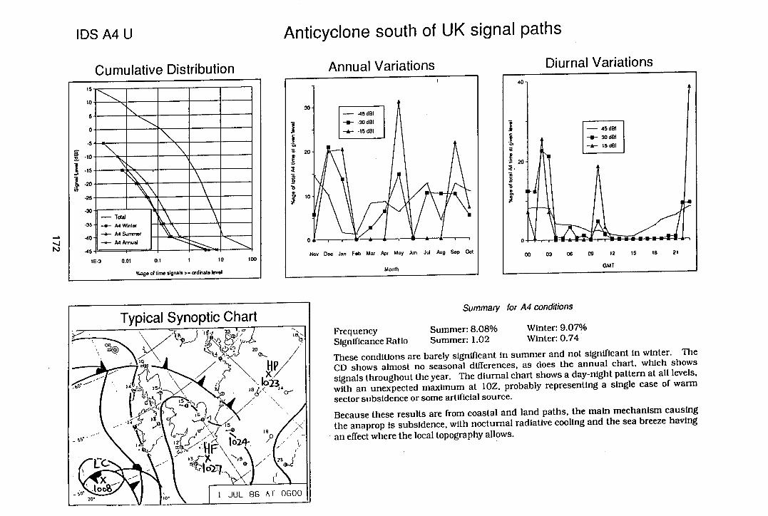
IDS A4U Anticyclone south of UK signal paths
Cumulative Distribution
Total __it__' !IlII% A4 Annual
Arrii,I VnrinfinnQ fli,irrI /iritinnQ
-4
Summary for A4 conditions
Frequency Summer: 8.08% Winter: 9.07%
Significance Ratio Summer: 1.02 Winter: 0.74
These conditions are barely significant in summer and not significant in winter. The CD shows almost no seasonal differences, as does the annual chart, which shows signals throughout the year. The diurnal chart shows a day-night pattern at all levels, with an unexpected maximum at 10Z. probably representing a single case of warm sector subsidence or some artificial source.
Because these results are from coastal and land paths, the main mechanism causing the anaprop is subsidence, with nocturnal radiative cooling and the sea breeze having an effect where the local topography allows.
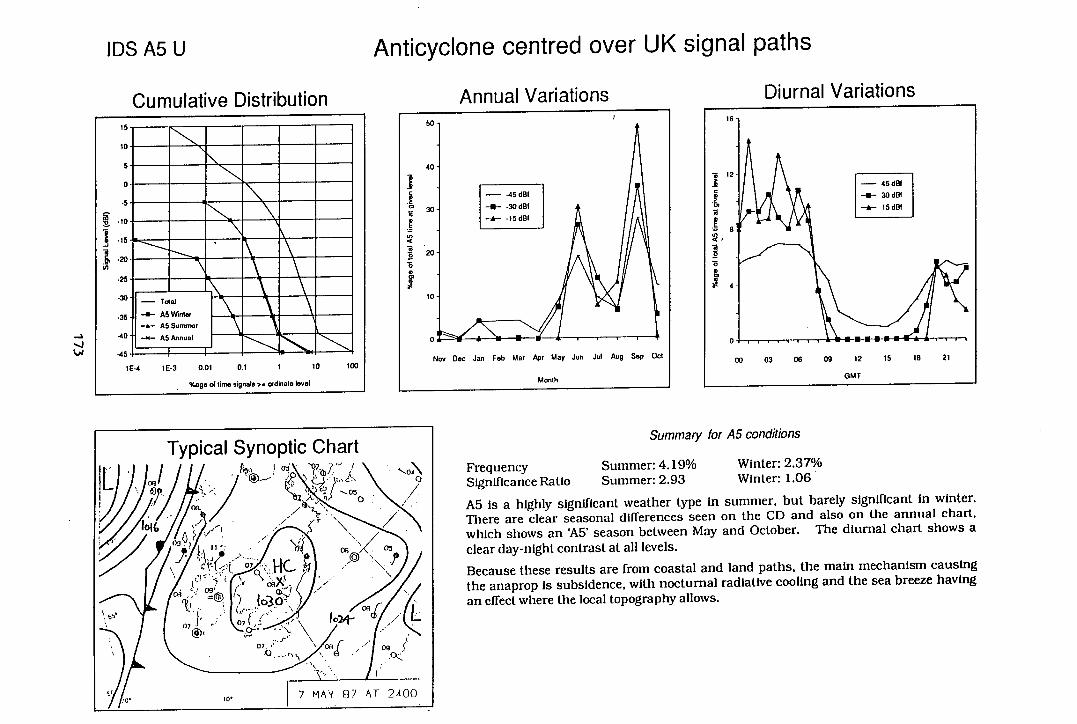
I-ri.,+irric
—a
IDS A5U
Cumulative Distribution
MINI ' I-
- ml AS
AS Sunnnner
nual
•__
Anticyclone centred over UK signal paths
r;..rI I!iritirflQ
Summary for A5 conditions
Frequency Summer: 4.19% Winter: 2.37%
Significance Ratio Summer: 2.93 Winter: 1.06
A5 is a highly significant weather type in summer, but barely significant in winter. There are clear seasonal differences seen on the CD and also on the annual chart, which shows an A5' season between May and October. The diurnal chart shows a clear day-night contrast at all levels.
Because these results are from coastal and land paths, the main mechanism causing the anaprop is subsidence, with nocturnal radiative cooling and the sea breeze having an effect where the local topography allows.
Typical Synoptic Chart
03
14c-
Oka
07 07 lox-
07. 0
J .
to- A7 AT 2A00
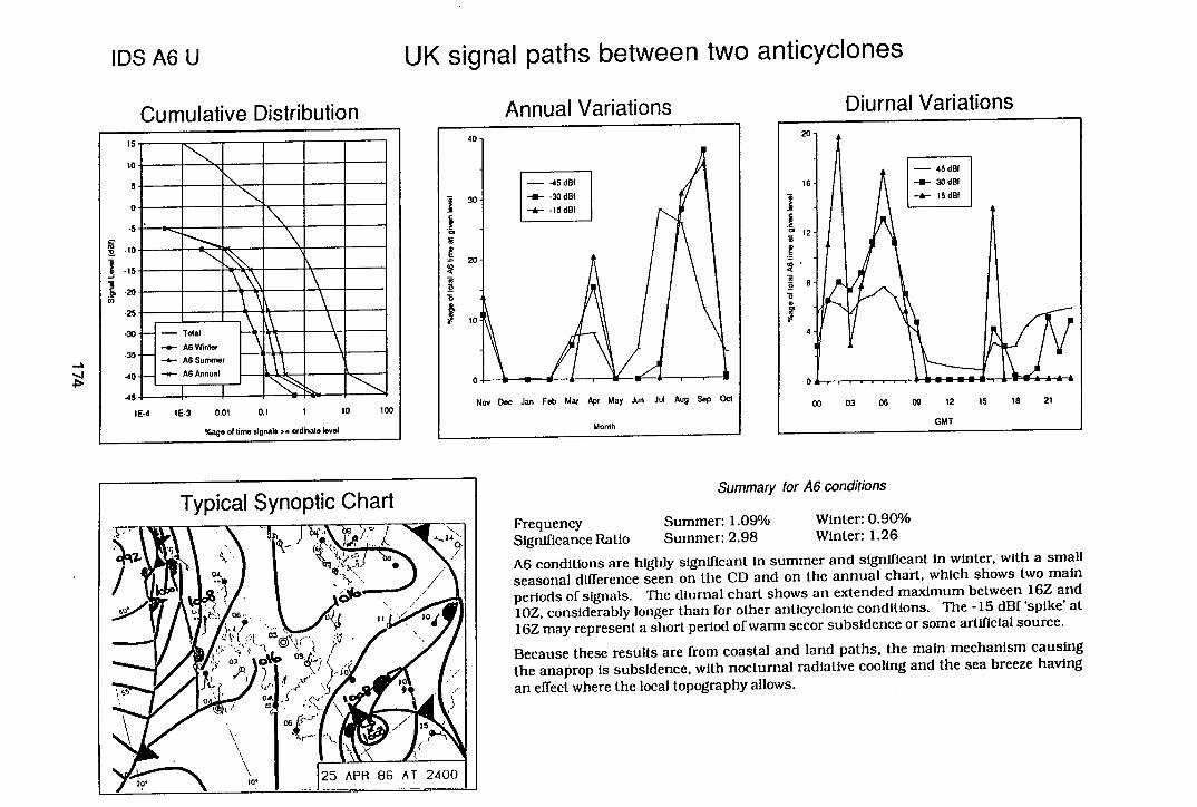
Cumulative Distribution
- - I
MM • __
III—MME A6 Summer A6 Annual
AO aWlinler
A 1.IrrI /irtirflQ
-
IDS A6U UK signal paths between two anticyclones
Typical Synoptic Chart
04.
-. 1• {J
'be
• //
.1 0 4 097/
06
\ 25 APR 86 AT 2400
Summary for A6 conditions
Frequency Summer: 1.09% Winter: 0.90%
Significance Ratio Summer: 2.98 Winter: 1.26
A6 conditions are highly significant in summer and significant in winter, with a small seasonal difference seen on the CD and on the annual chart, which shows two main periods of signals. The diurnal chart shows an extended maximum between 16Z and 10Z, considerably longer than for other anticyclonic conditions. The -15 dBf 'spike' at 16Z may represent a short period of warm secor subsidence or some artificial source.
Because these results are from coastal and land paths, the main mechanism causing the anaprop is subsidence, with nocturnal radiative cooling and the sea breeze having an effect where the local topography allows.
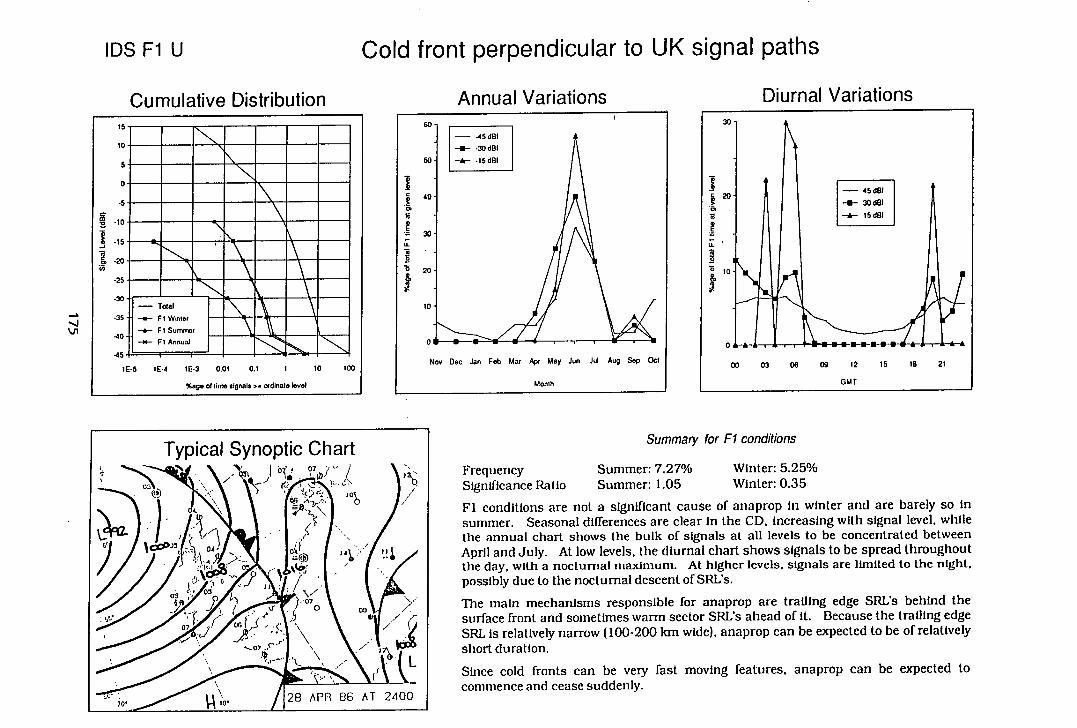
IDS F1
Cold front perpendicular to UK signal paths
Cumulative Distribution Armi ,I \/rktirnQ fliiirnI \/rLtinnc
—a Total _II'I'1I
-lIiI ,t1--I
Summary for Fl conditions
Frequency Summer: 7.27% Winter: 5.25% Significance Ratio Summer: 1.05 Winter: 0.35
Fl conditions are not a significant cause of anaprop In winter and are barely so in summer. Seasonal differences are clear in the CD, increasing with signal level, while the annual chart shows the bulk of signals at all levels to be concentrated between April and July. At low levels, the diurnal chart shows signals to be spread throughout the day, with a nocturnal maximum. At higher levels, signals are limited to the night, possibly due to the nocturnal descent of SRL's.
The main mechanisms responsible for anaprop are trailing edge SRL's behind the surface front and sometimes warm sector SRL's ahead of it. Because the trailing edge SRL Is relatively narrow (100-200 kin wide), anaprop can be expected to be of relatively short duration.
Since cold fronts can be very fast moving features, anaprop can be expected to commence and cease suddenly.
Typical Synoptic Chart
05
I Job
N
I
04- J4
03 03 it
70,
/ 28 APR 86 AT 2400
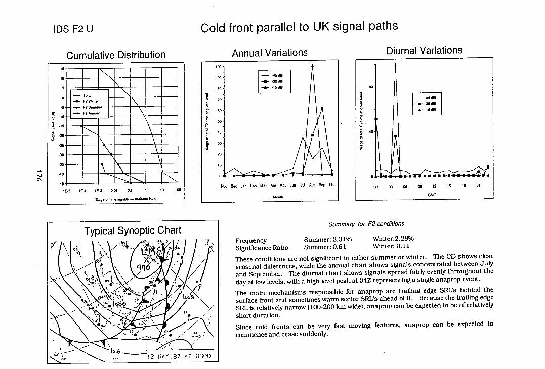
IDS F2U
Cold front parallel to UK signal paths
-
-4 CN
Cumulative Distribution
MM
w- F2 Winter
F2 Suntrne
INEENEENE
AnniiI /ritinnc fli .rnI Vnrintinnz
Typical Synoptic Chart
Y., \
\/ ). j I: 30
90
30
7? °Itoo ,
-
12 MAY 87 AT 0600
Summary for F2 conditions
Frequency Summer: 2.31% Winter:2.28%
Significance Ratio Summer: 0.61 Winter: 0.11
These conditions are not significant in either summer or winter. The CD shows clear seasonal differences, while the annual chart shows signals concentrated between July and September. The diurnal chart shows signals spread fairly evenly throughout the day at low levels, with a high level peak at 04Z representing a single anaprop event.
The main mechanisms responsible for anaprop are trailing edge SRL's behind the surface front and sometimes warm sector SRL's ahead of it. Because the trailing edge SRL is relatively narrow (100-200 km wide), anaprop can be expected to be of relatively short duration.
Since cold fronts can be very fast moving features, anaprop can be expected to commence and cease suddenly.
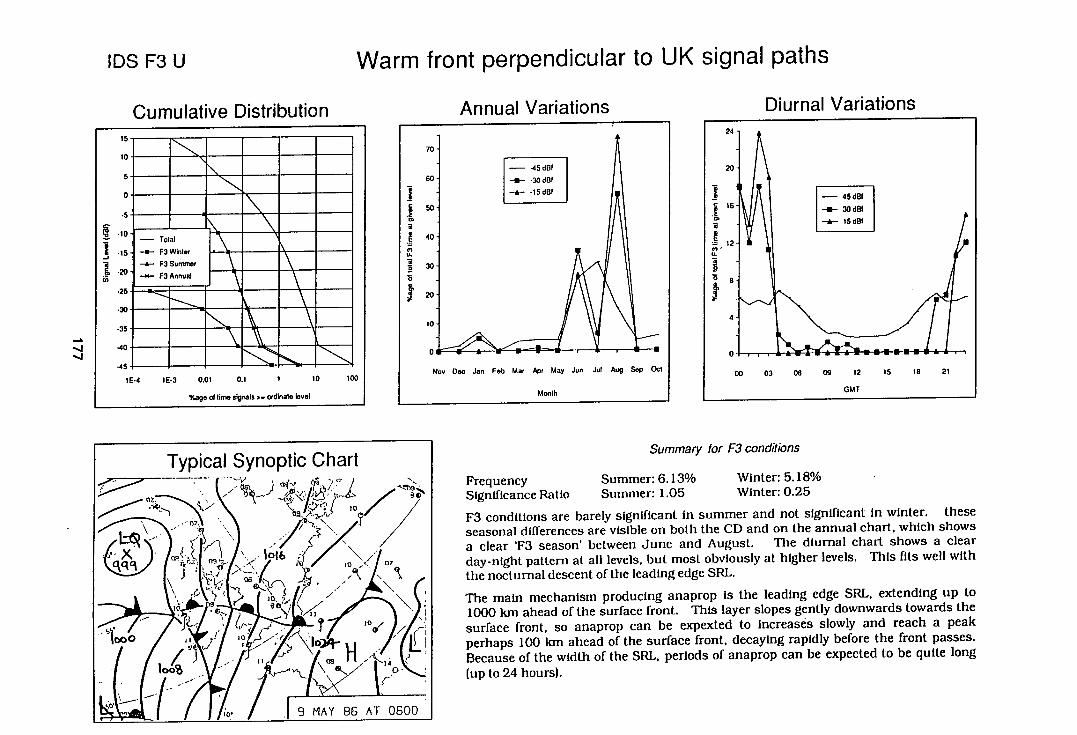
IDS F3U
Warm front perpendicular to UK signal paths
—a -.4 —S
Cumulative Distribution
Total
F3 Suntrmr Slim Ann _
NO- _
Anni iI /ritinnc fli irnI Vnrinfinncz
Typical Synoptic Chart
Lq
()
'
—iL' /JSç
10
• '7° 7 i!d. H 2VQ o/
9 MAY 86 AT 0600
Summary for F3 conditions
Frequency Summer: 6.13% Winter: 5.18% Significance Ratio Summer: 1.05 Winter: 0.25
F3 conditions are barely significant in summer and not significant in winter, these seasonal differences are visible on both the CD and on the annual chart, which shows a clear 73 season' between June and August. The diurnal chart shows a clear day-night pattern at all levels, but most obviously at higher levels. This fits well with the nocturnal descent of the leading edge SRL.
The main mechanism producing anaprop is the leading edge SRL, extending up to 1000 km ahead of the surface front. This layer slopes gently downwards towards the surface front, so anaprop can be expexted to increases slowly and reach a peak perhaps 100 km ahead of the surface front, decaying rapidly before the front passes. Because of the width of the SRL, periods of anaprop can be expected to be quite long (up to 24 hours).
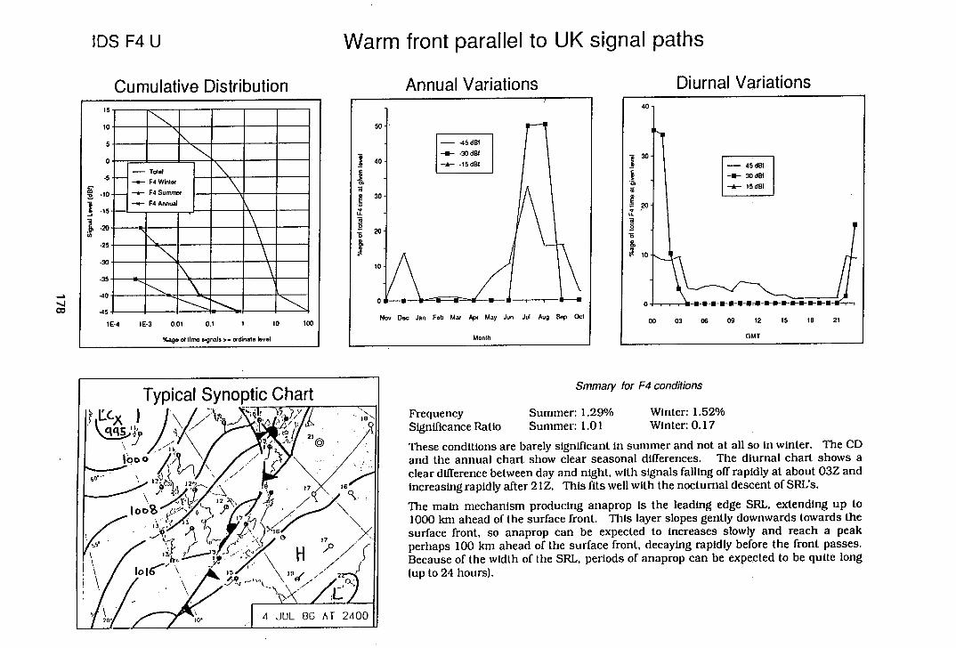
MMM MMMMMMM MMMMMM
Tdw
F4 AnnuW
•iuUi
-
' I _
-'
MILE ==Kim MMIUMM _1
IDS F4U
Warm front parallel to UK signal paths
Cumulative Distribution
Annual Variations Diurnal Variations
Typical Synoptic Chart qS
000
JV 17
17
17
p
\ \ /
f55
H '1 \ / Io( \
\/ 7 OA
f/ ,-7. 4 JUL 86 AT 2400
Smmary for F4 conditions
Frequency Summer: 1.29% Winter: 1.52% Significance Patio Summer: 1.01 Winter: 0.17
These conditions are barely significant In summer and not at all so in winter. The CD and the annual chart show clear seasonal differences. The diurnal chart shows a clear difference between day and night, with signals falling off rapidly at about 03Z and Increasing rapidly after 21Z. This fits well with the nocturnal descent of SRCs.
The main mechanism producing anaprop Is the leading edge SRL, extending up to 1000 km ahead of the surface front. This layer slopes gently downwards towards the surface front, so anaprop can be expected to increases slowly and reach a peak perhaps 100 km ahead of the surface fr ont, decaying rapidly before the front passes. Because of the width of the SRL, periods of anaprop can be expected to be quite long (up to 24 hours).
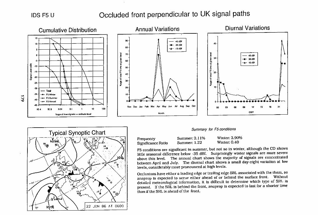
IDS F5U
Occluded front perpendicular to UK signal paths
'0
Cumulative Distribution
MM =MM _________I
TOW
FS Wint6r
FS Summer all
ft i-in. Irktirnc fliirrI Irfrnc
Typical Synoptic Chart 33 ,
10
OS; 36
22
20 0. "' 1 22 JUN 86 AT 0600
Summary for F5 conditions
Frequency Summer: 2.11% Winter: 2.90% Significance Ratio Summer: 1.22 Winter: 0.40
F5 conditions are significant in summer, but not so In winter, although the CD shows little seasonal difference below -35 dIM. Surprisingly winter signals are more severe above this level. The annual chart shows the majority of signals are concentrated between April and July. The diurnal chart shows a small day-night variation at low levels, considerably more pronounced at high levels.
Occlusions have either a leading edge or trailing edge SRL associated with the them, so anaprop is expected to occur either ahead of or behind the surface front. Without detailed meteorological information, it Is difficult to determine which type of SRL is present. If the SRI. Is behind the front. anaprop Is expected to last for a shorter time than if the SRL Is ahead of the front.
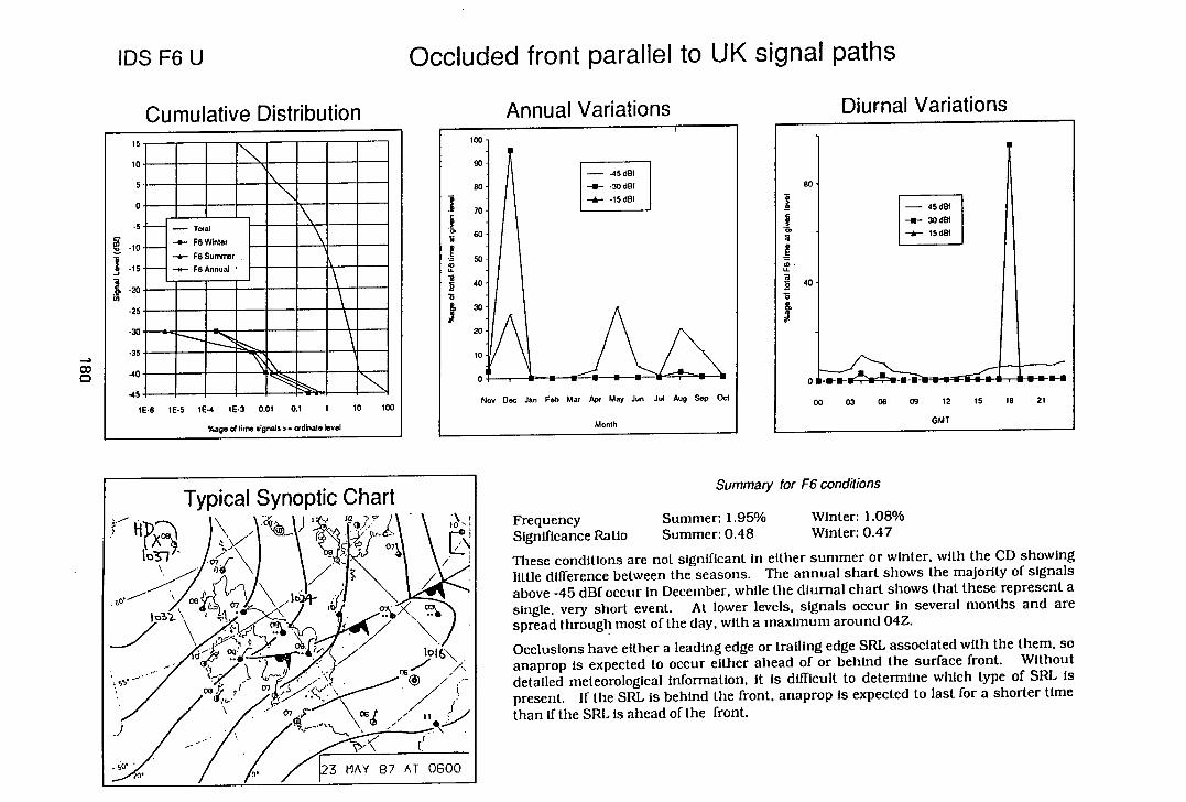
IDS F6U
Occluded front parallel to UK signal paths
-
0
Cumulative Distribution
111111111111111111111110111 mom woommoom
-a- RlNintar
IUA'iIUflI woommal
Annual Variations fliiirnI Vritions
/•( II
Typical Synoptic Chart 1420 F
Lo7 - ioir\ i
<'4 L toO7. (
I
\7 07
Summary for F6 conditions
Frequency Summer: 1.95% Winter: 1.08% Significance Ratio Summer: 0.48 Winter: 0.47
These conditions are not significant in either summer or winter, with the CD showing little difference between the seasons. The annual shart shows the majority of signals above -45 dBf occur in December, while the diurnal chart shows that these represent a single, very short event. At lower levels, signals occur in several months and are spread through most of the day, with a maximum around 04Z.
Occlusions have either a leading edge or trailing edge SRL associated with the them, so anaprop is expected to occur either ahead of or behind the surface front. Without detailed meteorological Information. It is difficult to determine which type of SRL Is present. If the SRL Is behind the front. anaprop is expected to last for a shorter time than If the SRL Is ahead of the front.
MAY 87 AT 0600
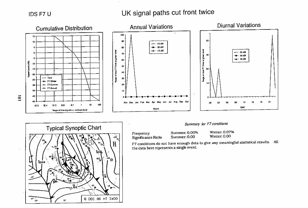
IDS F7U UK signal paths cut front twice
Cumulative Distribution
-
AnniiI Vn rinfinn.q fliiirn& \/iritinnc
Typical Synoptic Chart
034 ~11
10 00
-04
10
07
08 CY7 13
\
°• 8 DEC 86 AT 2400 -
Summary for F7 conditions
Frequency Summer: 0.00% Winter: 0.07%
Significance Ratio Summer: 0.00 Winter: 0.00
F7 conditions do not have enough data to give any meaningful statistical results. All the data here represents a single event.
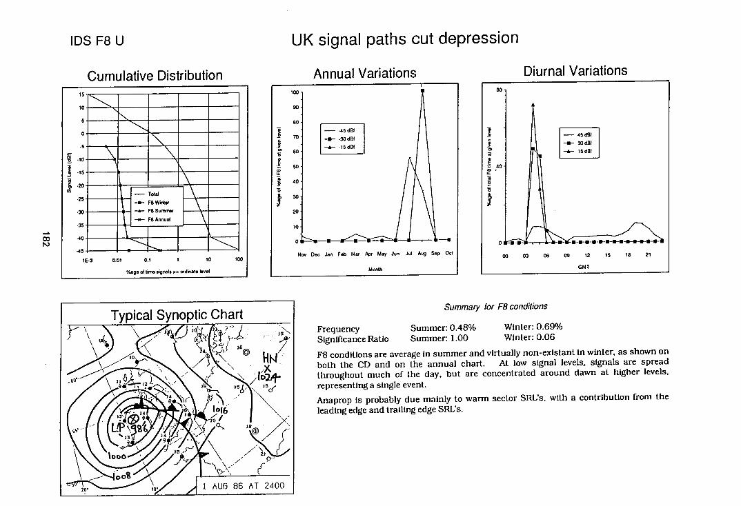
IDS F8U
Cumulative Distribution
ff..i RAnnual
_I— . _
scm - CO
UK signal paths cut depression
A _. ._I V flu irr%1I /rifirtnc
Typical Synoptic Chart
02+ 12 15
Is 39
1000 "" \\21/
002
20* 10, 1 AUG 86 AT 2400
V Summary for F8 conditions
Frequency Summer: 0.48% Winter: 0.69% Significance Ratio Summer: 1.00 Winter: 0.06
F8 conditions are average in summer and virtually non-existant in winter, as shown on both the CD and on the annual chart. At low signal levels, signals are spread throughout much of the day, but are concentrated around dawn at higher levels, representing a single event.
Anaprop is probably due mainly to warm sector SRL's, with a contribution from the leading edge and trailing edge SRL's.
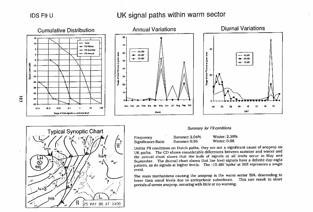
Cumulative Distribution
- m,_iI owl
I I-
Annual Variations Diurnal Variations
-
IDS F9U
UK signal paths within warm sector
Summary for F9 conditions
Frequency Summer: 2.04% Winter: 2.39% Significance Ratio Summer: 0.95 Winter: 0.08
Unlike F9 conditions on Dutch paths, they are not a significant cause of anaprop on UK paths. The CD shows considerable differences between summer and winter and the annual chart shows that the bulk of signals at all levels occur In May and September. The diurnal chart shows that low level signals have a definite day-night pattern, as do signals at higher levels. The -15 dBf 'spike' at 20Z represents a single event.
The main mechanisms causing the anaprop is the warm sector SRL descending to lower then usual levels due to anticyclonic subsidence. This can result In short periods of severe anaprop, occuring with little or no warning.
Typical Synoptic Chart 09
14 H 02"iY j/.(
:.s'\ 12. 10' ' 00
09 12
12
I002 -P'09 ,c- /
/ \
IS,
1016 Th(L y 10 / J25 MAY 86 AT 2400
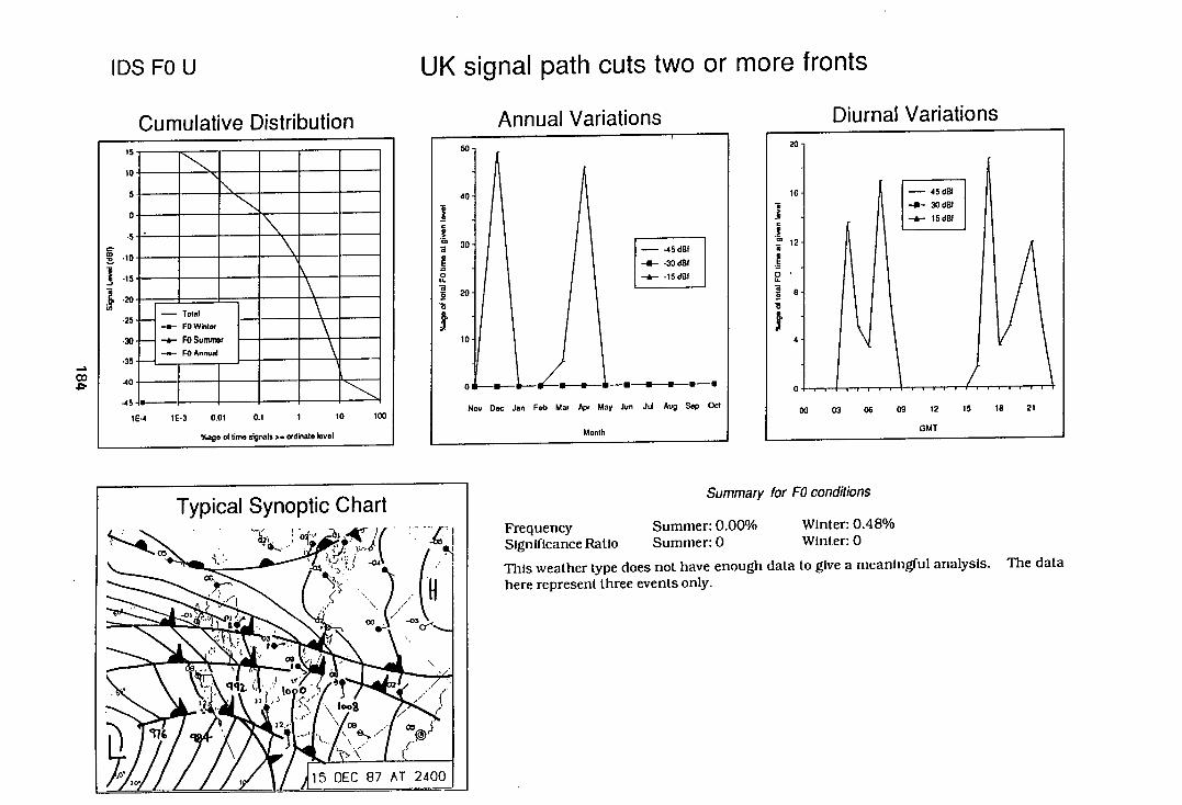
Ar,,, ..I
Ir*rie.
IDS FOU
UK signal path cuts two or more fronts
— CO
Cumulative Distribution
----
• • I —.__ EM all 0 , FOWinte,
• I' FO SUMMr FO AnnuaJ
MMM
Typical Synoptic Chart
f'.1
oo
\\ \.
oO/ -
176
15 DEC 87 AT 24001
Summary for FO conditions
Frequency Summer: 0.00% Winter: 0.48% Significance Ratio Summer: 0 Winter: 0
This weather type does not have enough data to give a meaningful analysis. The data here represent three events only.
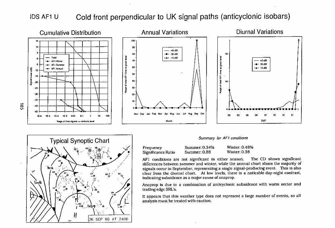
IDS AR U Cold front perpendicular to UK signal paths (anticyclonic isobars)
Cumulative Distribution
Annual Variations
Diurnal Variations
AF Annual'
L MM
MMMMMMMM MMMMMMMM MMMMMMM MMNLMNIMMM
Typical Synoptic Chart
09
00
104 7 2
i,5 / 08
M 09
'A ': r/L 13
126 SEP 88 AT 2400 to.
Summary for AF1 conditions
Frequency Summer: 0.34% Winter: 0.48% Significance Ratio Summer: 0.88 Winter: 0.38
AF1 conditions are not significant in either season. The CD shows significant differences between summer and winter, while the annual chart shoes the majority of signals occur in September, representing a single signal-producing event. This is also clear from the diurnal chart. At low levels, there is a noticable day-night contrast. Indicating subsidence as a major cause of anaprop.
Anaprop is due to a combination of anticyclonic subsidence with warm sector and trailing edge SRL's.
It appears that this weather type does not represent a large number of events, so all analysis must be treated with caution.
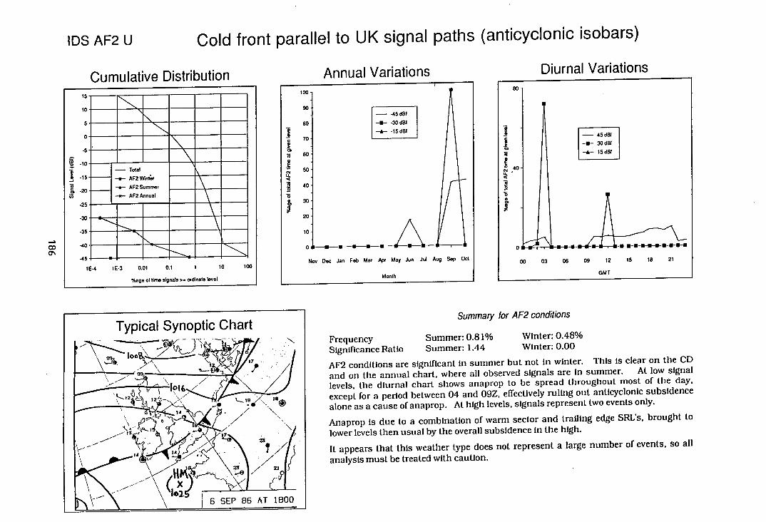
IDS AF2 U Cold front parallel to UK signal paths (anticyclonic isobars)
Cumulative Distribution
•i —I
A rrI iI /rkitirnc ri;. lIri+irnc
-
Summary for AF2 conditions
Frequency Summer: 0.8 1% Winter: 0.48%
Significance Ratio Summer: 1.44 Winter: 0.00
AF2 conditions are significant in summer but not in winter. This is clear on the CD and on the annual chart, where all observed signals are in summer. At low signal levels, the diurnal chart shows anaprop to be spread throughout most of the day. except for a period between 04 and 09Z. effectively ruling out anticyclonic subsidence alone as a cause of anaprop. At high levels, signals represent two events only.
Anaprop is due to a combination of warm sector and trailing edge SRL's, brought to lower levels then usual by the overall subsidence in the high.
It appears that this weather type does not represent a large number of events, so all analysis must be treated with caution.
Typical Synoptic Chart
TI Igo
IA
--.-' 23
23
X
6 SEP 86 AT 1800
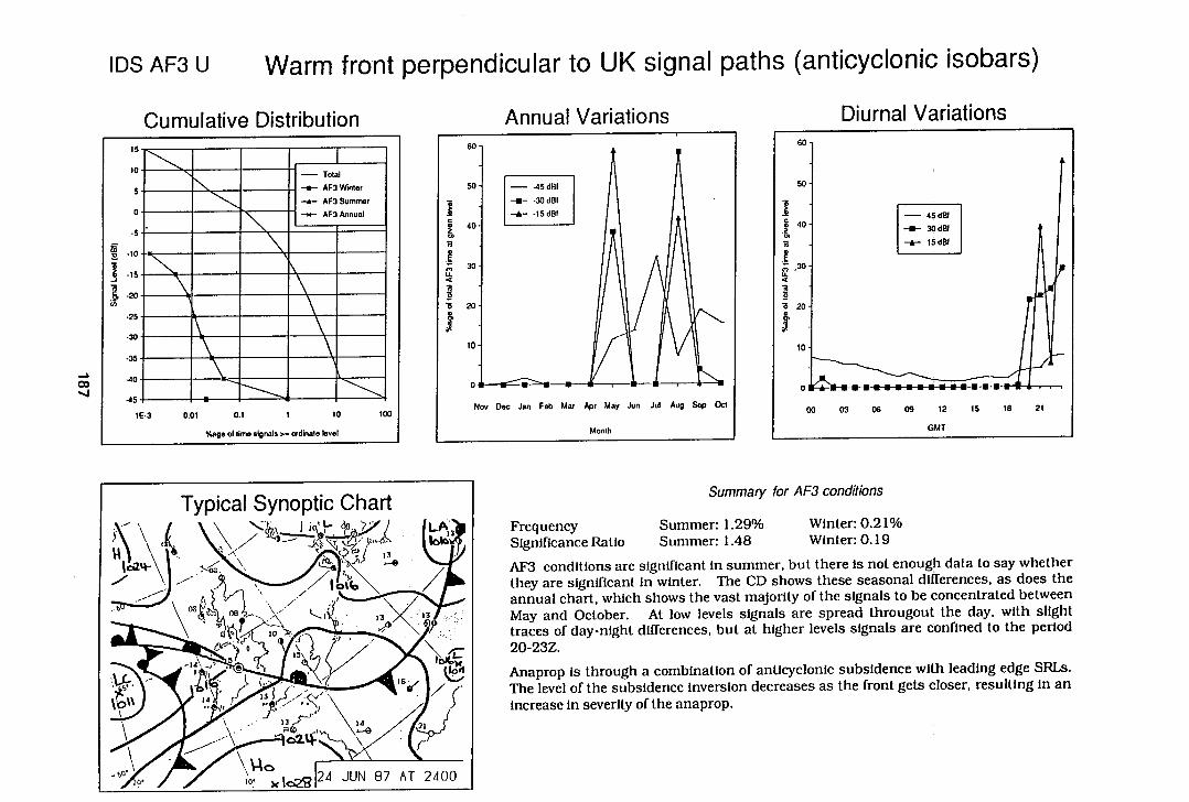
IDS AF3 U Warm front perpendicular to UK signal paths (anticyclonic isobars)
Cumulative Distribution A ..
CID
1 IiI
Typical Synoptic Chart
13
J_~ L \•,/ (—c\ //444_. 13 13
30
Summary for AF3 conditions
Frequency Summer: 1.29% Winter: 0.2 1% Significance Ratio Summer: 1.48 Winter: 0.19
AF3 conditions are significant in summer, but there is not enough data to say whether they are significant In winter. The CD shows these seasonal differences, as does the annual chart, which shows the vast majority of the signals to be concentrated between May and October. At low levels signals are spread througout the day, with slight traces of day-night dilTerences, but at higher levels signals are confined to the period 20-23Z.
Anaprop is through a combination of anticyclonic subsidence with leading edge SRLs. The level of the subsidence inversion decreases as the front gets closer, resulting in an Increase in severity of the anaprop.
36
-
IT )(
[24 AT 2400
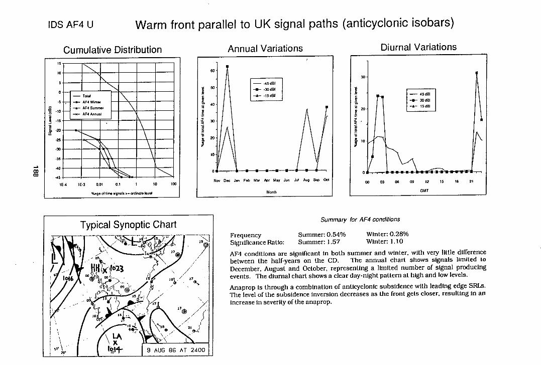
Cumulative Distribution
- I
I I IiIII__. IIu- Total AF4 Winter
R Anu.L_1 '_ _ MMMMIMMM I MMMMILM I
__
M 1611-IM
__ - I
•__
A .tI I-tr;_tf;rtrc
co
is:. I;;rtr'
IDS AF4 U Warm front parallel to UK signal paths (anticyclonic isobars)
Typical Synoptic Chart
17
07
Vk iv1T:" 1o16 39 / 37
VI k 17 / 10j ç\( \ /
/ 18Ø
\ 23j
I (\" ( Ilf 9 AUG 86 AT 2400 20,
Summary for AF4 conditions
Frequency Summer: 0.54% Winter: 0.28% Significance Ratio: Summer: 1.57 Winter: 1.10
AF4 conditions are significant In both summer and winter, with very little difference between the half-years on the CD. The annual chart shows signals limited to December, August and October, representing a limited number of signal producing events. The diurnal chart shows a clear day-night pattern at high and low levels.
Anaprop is through a combination of anticyclonic subsidence with leading edge SRLs. The level of the subsidence inversion decreases as the front gets closer, resulting in an increase in severity of the anaprop.
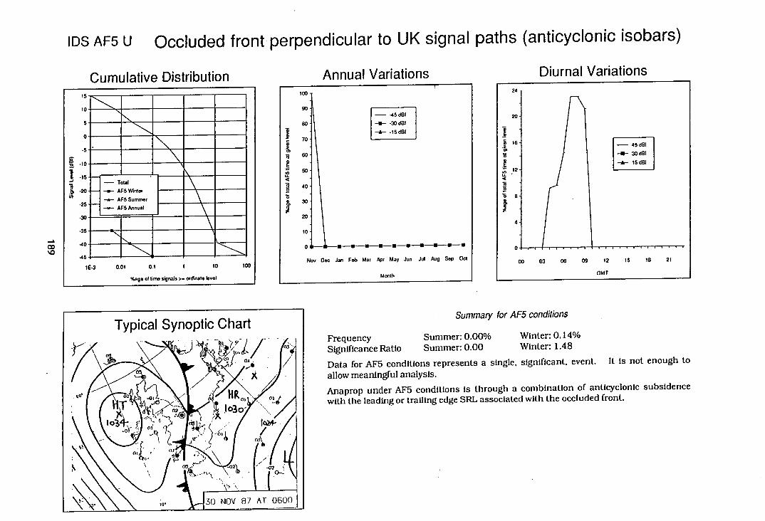
r:. A Cumulative Distribution
IS
to
5
o
.5
co .lo
-15
-20
25
- Total
AF5nter
-a- AF5 Summer \ i3
.35
-40
.45
10-3 001 0.1 1 10 100
%age of time signalos. ordinate level
IDS AF5 U Occluded front perpendicular to UK signal paths (anticyclonic isobars)
Summary for AF5 conditions
Frequency Summer: 0.00% Winter: 0.14%
Significance Ratio Summer: 0.00 Winter: 1.48
Data for AF5 conditions represents a single, significant, event. It is not enough to allow meaningful analysis.
Anaprop under AF5 conditions Is through a combination of anticyclonic subsidence with the leading or trailing edge SRL associated with the occluded front.
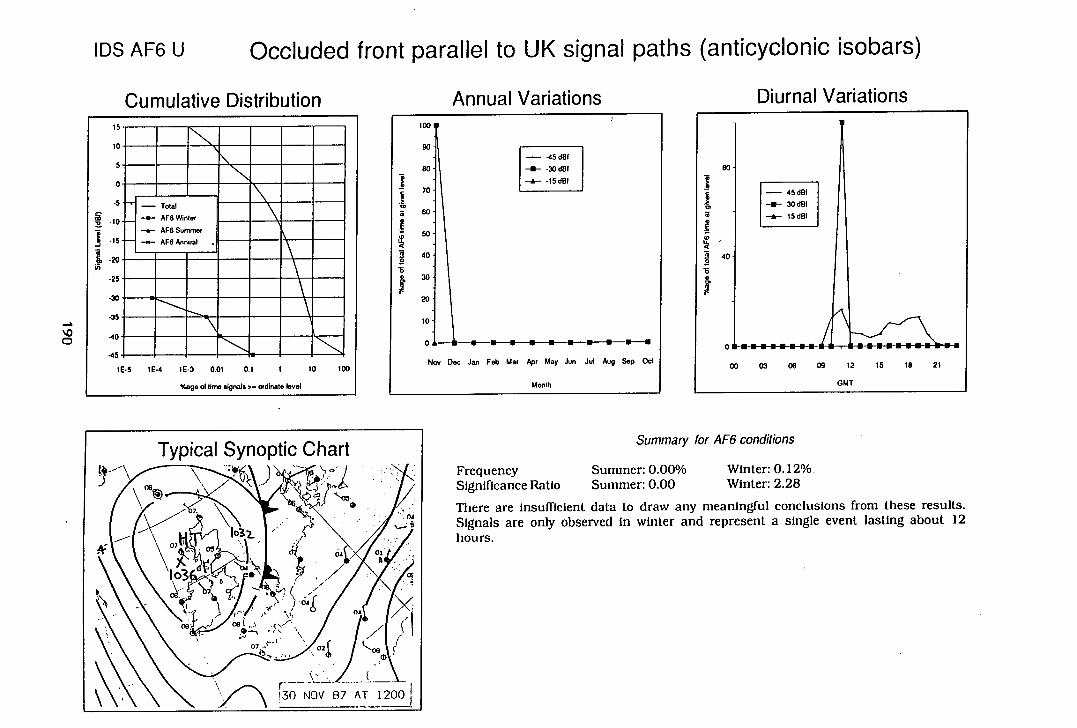
IDS AF6 U Occluded front parallel to UK signal paths (anticyclonic isobars)
Cumulative Distribution
Anniil Viritinns flu irniI Vriitinnc
.- '0 0
MMMMMMM MMMMMMM
Tota
AF6 Summer
• L MMMMMILIM
MMIMMMMI
Summary for AF6 conditions
Frequency Summer: 0.00% Winter: 0.12% Significance Ratio Summer: 0.00 Winter: 2.28
There are insufficient data to draw any meaningful conclusions from these results. Signals are only observed in winter and represent a single event lasting about 12 hours.
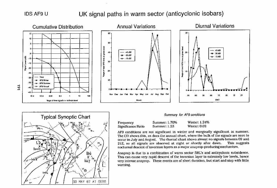
IDS AF9 U UK signal paths in warm sector (anticyclonic isobars)
Cumulative Distribution A.-.....-I r:.
— "C —'
• 0
--_ _
t.Il • Ifri l _
• I
Typical Synoptic Chart (\ \\/.\) 3QJ'J
\ - / c- •\ /
L 134.
'
c(
-00 09
bb i 2T 12
10 10
• . F3O MY 87 AT 0600
Summary for AF9 conditions
Frequency Summer: 1.70% Winter: 1.24% Significance Ratio Summer: 1.23 Winter: 0.02
AF9 conditions are not significant in winter and marginally significant In summer. The CD shows this, as does the annual chart, where the bulk of the signals are seen to occur in July and August. The diurnal chart shows almost no signals between 09 and 21Z, so all signals are observed at night or shortly after dawn. This suggests nocturnal descent of inversion layers as a major anaprop-producing mechanism.
Anaprop is due to a combination of warm sector SRL's and anticyclonic subsidence. This can cause very rapid descent of the inversion layer to extremely low levels, hence very intense anaprop. These events are of short duration, but start and stop with little warning.
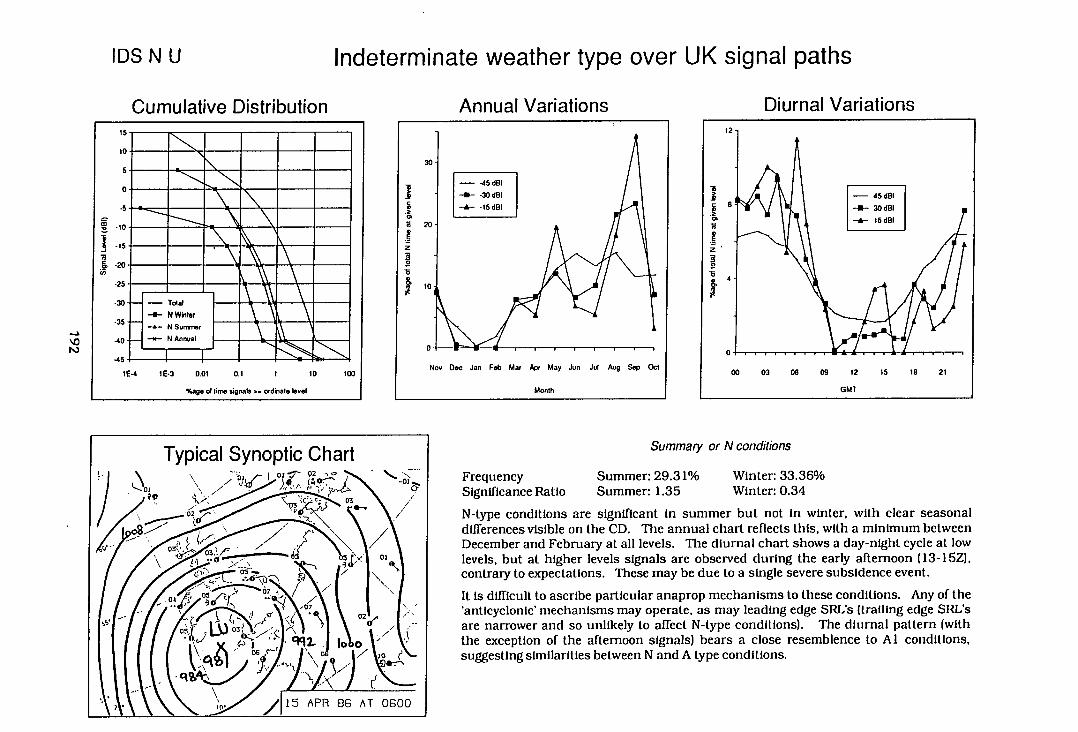
Typical Synoptic Chart \ '.--o
/ f \ ,•'
-: -S
U Cl
01
17
- A10
IDS N U
Indeterminate weather type over UK signal paths
Cumulative Distribution
Annual Variations
Diurnal Variations
-
'0 F..)
- -- I
II______
To N Winter II4i__I
Summary or N conditions
Frequency Summer: 29.3 1% Winter: 33.36% Significance Ratio Summer: 1.35 Winter: 0.34
N-type conditions are significant in summer but not in winter, with clear seasonal differences visible on the CD. The annual chart reflects this, with a minimum between December and February at all levels. The diurnal chart shows a day-night cycle at low levels, but at higher levels signals are observed during the early afternoon (13-15Z), contrary to expectations. These may be due to a single severe subsidence event.
It Is difficult to ascribe particular anaprop mechanisms to these conditions. Any of the 'anticyclonic' mechanisms may operate, as may leading edge SRL's (trailing edge SRL's are narrower and so unlikely to affect N-type conditions). The diurnal pattern (with the exception of the afternoon signals) bears a close resemblence to Al conditions, suggesting similarities between N and A type conditions.
15 APR 86 AT 0600

Appendix B
Publications and reports
B.1 Reports
This section lists (chronologically) all reports written by the author during the research
for this thesis and gives a. short summary of each. Reports are unpublished unless
otherwise indicated and in all cases copies are available from:
Department of Meteorology
Kings Buildings
University of Edinburgh
EDINBURGH
E119 3JZ
SCOTLAND
or from:
Antenna and Spectrum Management Group
BTL
Martlesham Heath
IPSWICH
1P5 7RE
ENGLAND
193
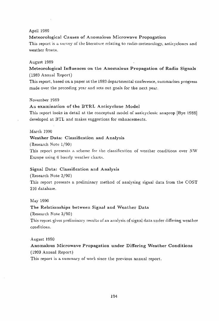
April 1989
Meteorological Causes of Anomalous Microwave Propagation
This report is a survey of the literature relating to ra.dio-meteorology, anticyclones and
weather fronts.
August 1989
Meteorological Influences on the Anomalous Propagation of Radio Signals
(1989 Annual Report)
This report, based on a paper at the 1989 departmental conference, summarises progress
made over the preceding year and sets out goals for the next year.
November 1989
An examination of the BTRL Anticyclone Model
This report looks in detail at the conceptual model of anticyclonic anaprop [Bye 19881
developed at BTL and makes suggestions for enhancements.
March 1990
Weather Data: Classification and Analysis
(Research Note 1/90)
This report presents a scheme for the classification of weather conditions over NW
Europe using 6 hourly weather charts.
Signal Data: Classification and Analysis
(Research Note 2/90)
This report presents a preliminary method of analysing signal data from the COST
210 database.
May 1990
The Relationships between Signal and Weather Data
(Research Note 3/90)
This report gives preliminary results of an analysis of signal data under differing weather
conditions.
August 1990
Anomalous Microwave Propagation under Differing Weather Conditions
(1990 Annual Report)
This report is a summary of work since the previous annual report.
194

April 1991
The Role of Fronts in Anomalous Microwave Propagation
Paper presented at Seventh International Coii Ieieiice oti Antennas and Propagation
(ICAP'91)
York University, April 1991
Published in Inst. Elec. Eng. Conf. Pub. 333 Part 1; p 185-8 A copy of this paper is given immediately after this section.
August 1991
Conceptual Models of the Radio-Meteorology of Fronts
This report (effectively chapter 4 of this thesis) presents the conceptual models of
fronts.
December 1991
Draft Final Report
This report, for BTL, gives the final state of the different goals of the research contract
and presents chapters 4 and 5 of this thesis.
January 1993
Interference Data Sheet Portfolio
This is identical to the set of IDSs presented in appendix A of this thesis.
B.2 Published Papers
The following is a copy of a paper by the author presented at ICAP'91 and published in
the conference proceedings. The author would like to thank the Institute of Electrical
Engineers for permission to reproduce the work.
195
185
THE ROLE OF FRONTS IN ANOMALOUS MICROWAVE PROPAGATION
T Jones
University of Edinburgh, UK
INTRODUCTION
The weather has an important influence on radio communications links, both when choosing a suitable path for a new link and when a link is operational. A good understanding of the effects of different atmospheric conditions on signal propagation is therefore vital to telecommunications organisations. The mechanisms that lead to anomalous propagation (anaprop) . mainly through ducting - are well understood, as is the occurrence of anomalous propagation during anticyclonio conditions (1). Since anaprop is not confined to anti-cyclones, it is necessary to look at the effects of other weather conditions on propagation, in particular that of weather fronts and the interactions between fronts and anticyclones.
This paper examines these relatively unstudied aspects of radio-meteorology in several ways. A brief account of previous work on the radio-meteorology of fronts is followed by a statistical analysis of their effects on propagation on a number of links in NW Europe. A conceptual model of the radio-meteorology of fronts is presented as are some case studies of signal behaviour under a variety of weather conditions. This work has been approached from the point of view of a meteorologist, so should offer a different approach to the study of anomalous propagation.
This work is carried out under contract to British Telecom Research Laboratories (BTRL). Acknowledgement is made to the Director of Research and Technology Department of British Telecom for permis-sion to publish this paper.
FRONTS AND PROPAGATION
In the past. most radio-meteorologists have concentrated on the mechanisms responsible for anaprop, or on its occurrence during anticyclones, with relatively little attention being paid to fronts. Given the transitory nature of fronts, and the resulting difficulty in obtaining good data on the refractivity structure aloft, this is not unreasonable. Several authors, however, have mentioned that fronts have some effect on signals, but have not gone into much more detail.
Bean & Dutton (21 cite an earlier study that showed a rapid drop in signal levels when a cold front moved over a link. This is supported by Kuhn & Ogulwi (31 which found that signal levels increased with the passage of some warm fronts and decreased when some cold fronts passed. The work only examined the most severe instances of frontal snaprop, supporting the differences between ana- and kate- type fronts discussed later in this work.
Bean & Dutton's analysis of surface refractive index charts (2) showed higher levels in the warm sector than ahead and behind the depression, but again this was only a single case study. Cross sections through a cold front (21 showed that refractivity isopleths were lower immediately ahead of the front than behind or further ahead of it. A similar analysis (4) looked at two exceptionally severe events, involving interactions between fronts and anticyclones. As they coincided with routine upper air observations, detailed examinations of the refractivity structure were possible. It was found that the anaprop was due to the abrupt descant of a subsidence inversion (and the associated duct) from its usual level near 2000m to as low as 500m, albeit for a short period. This phenomenon, termed 'sporadic sub-sidence' by BTRL was used as the basis of the F9 and AF9 weather classes used later in this work.
A recent statistical analysis (51 found that high signal levels were more common than usual when a link was immediately ahead of a warm front or immediately behind a cold front. This also agrees with the conceptual model presented here.
STATISTICAL ANALYSIS
Using data from a number of signal paths in the UK and across the southern North Sea (Fig 11, data for the whole of 1986 and 1987 were examined and correlated with the prevailing weather conditions. Weather information was obtained from charts, produced by the UK Meteorological Office every six hours, and each chart was classified
according to the presence of anticyclones and fronts using the scheme illustrated in Fig 2. The anticyclonic (A) weather classes are based on the BTRL conceptual model of anticyclonic anaprop, extended to take account of different possible locations of the high pressure centre relative to the link. Frontal (F) weather classes 1 to 6 are based on the conceptual model presented here and F9 is based on the 'sporadic subsidence' mechanism of Hewitt at of 141. The other F weather classes were added to the scheme to account for some of the more unusual weather types observed. Interactions between anticyclones and fronts (AF classes) correspond to the matching F class, but with anticyclonic curvature of the isobars on the chart. A final class (N) accounts for periods when neither fronts nor anticyclones affected a region. Weather conditions were classified separately for the UK, Dutch and Channel Island 'zones' indicated on Fig 1. To account for seasonal effects, both weather and signal data were split into winter (November to April) and summer (May to October) half years, based on the annual temperature cycle.
Signal data was in the form of the time (in seconds) signals exceeded thresholds (at 5 dflf intervals) each hour. To give a single index of the signal behaviour, the data were converted to a significant signal level'. This is defined as the lowest level that there are more signals than a critical limit (10 seconds at 60 dBf below free space, decreasing linearly to 0 seconds at the free space level) during the six hour period corraponding to a given weather chart. For instance, at 30 dBf below free space. 5 seconds or more of signals in six hours are needed for that level to be considered significant. Results were tabulated by weather type and significant level, allowing summary tables for each path to be produced. It was found that there was a close correlation between signals in each zone, so data were grouped into Dutch and UK (including Channel Islands) areas to give the final summaries (Figs 3a.b). These show the percentage of cases of each weather type that gave significant signals, irrespective of signal level, both for the summer and winter seasons, and for the whole year. For reference, the annual average significant percentage is shown as a line on each chart, the difference between the Dutch and UK values is due to a single UK path which is nearly in line of sight of the transmitter. Note that this aproach to the analysis ignores the severity of the signals but, as the paths used were all 'over-the-horizon' experimental links, any signals received on such a path would cause probably interference on an operational link. An examination of the severity of the signals showed a good connection to the significance, in that high significant percentages gave high signal levels.
It is clear from the charts that there are large variations in the signals, both between different weather types and seasons. Anti-cyclonic conditions are clearly a major cause of anaprop, but there are considerable differences between the Al and A3 classes on the one hand and the A2 and A4 ones on the other. This is due to the location of the paths, in the former case air arrives over the links after an overland path, thus advection ducting plays an important part, while in the latter case, air has a long track over the North Sea, minimising advection ducting. The observed results for anticyclonic conditions could thus not be expected to apply to regions other than NW Europe.
Frontal conditions appear to cause less than average amounts of anaprop, although there is a large variation between different types. There are no obvious patterns to the frontal interference, probably due to the large differences between individual fronts which cannot be captured in routine weather observations. The AF classes appear to follow the F classes, although significant percentages are higher, as if the anticyclonic circulation provides a 'background' with frontal effects superimposed on it. There are, however, relatively few cases of AF conditions, so the results may not be statistically significant. The F9 and the corresponding AF9 classes do appear to be significant, particularly on the sea paths to the Netherlands. The statistical significance of these results is currently being investigated.
196
186
A CONCEPTUAL MODEL OF FRONTS
Although conceptual models lack the 'glamour' of numerical models, they are an important tool for understanding the processes involved in any phenomenon. They also provide a framework for the interpretation of results and as a basis for more complex models. In meteorology there are two main models of the structure and processes of fronts and depressions. The Bergen model was developed in the 1920's and gave the picture of a frontal depression found in most meteorology texts (e.g. 61. This model is essentially static, giving 'snapshots' of a depression at different stages in its development. It also led to the idea of ana- and kata- type fronts, where sir is ascending or subsiding relative to the front respectivly. The second model is the Browning model, developed since the 1970's (7]. This model is dynamic, considering the airflows around depressions, and how their inter-actions lead to fronts.
This work takes elements of both the Bergen and Browning models and uses them to indicate the location of ducts near fronts. It is assumed that any subsided air will have a duct (or at least a super-refractive zone) at its base. The depressions shown here [Figs 4a,b] are good examples of ana- and kate-type fronts, but it must be stressed that few depressions are as clear-cut as these, and that individual fronts may exhibit both ana- and kate-type behaviour at different places.
The modal suggests that both ana- and kate-fronts have ducts immediately ahead of the surface warm front (WF) and just behind the surface cold front (CF). These are due to the 'dry zone' caused by subsiding air just beneath the frontal surface 161. Away from the surface fronts the ducts are high, but nearer the front the altitude is limited by the presence of the front, so the ducts slope gently downwards towards each front. Rain associated with the fronts is indicated on the diagrams since, although it has minimal effects at around 1 GHz, it may be important for work at other frequencies.
Kate-fronts are marked by a general subsidence in the warm sector, so a duct may exist over much of the depression. The duct is limited by the top of the warm conveyor belt (7), so as this rises up the WF, the duct is lifted. Some kate-type depressions have an upper cold front (IJCF) formed when instability in air in the warm conveyor belt causes convection. In this case the duct is broken into two sections at different heights [Fig 4b1 while if no UCF is present, the duct is continuous.
Clearly kate-fronts are more likely to cause anaprop than ana-fronts since there is a greater area of duct to intercept signals, so AF9 weather conditions, with subsidence in the warm sector due to the anticyclonic flow, can be expected to give a high incidence of anaprop (as the statistics showed). Some anaprop may be caused by ana-fronts, over short distances perpendicular to the fronts, as signal bounce off the duct to a receiver, and over longer distances parallel to the fronts as signals are trapped in the duct. Due to the speed with which fronts move (typically 10 to 20 ms- 1 ), such anaprop is likely to be of relatively short duration, while kate-fronts may cause longer periods of interference.
CASE STUDIES OF FRONTAL INTERFERENCE
A number of case studies are being made of events on a 66 km coastal link in SE England. Signal levels are sampled at lOs intervals to a resolution of Oj dBf, from which 5 minute means, maximum and minimum levels have been extracted. Weather data are available in the form of 6 hourly synoptic charts, as well as 12 hourly upper air observations. The studies cover a three month period in summer 1989 when a considerable amount of anaprop was observed. Two cases are examined in this work, the first shows enhanced signal levels apparently associated with the passage of a cold front while the second shows a particularly severe event that occurred during AF9 conditions.
During the CF event a front moved rapidly over the path and two periods of enhanced signals, each lasting some three hours, were observed. They are shown on Fig 5, together with the distance of the front from the transmitter. The data can be interpreted using the conceptual model of a kate front, although it is stressed that this interpretation has not yet been rigorously checked. The first period of enhancement (marked A on Fig 5) can be ascribed to the subsidence in the warm air ahead of the front. The drop in signal levels coincides with the passage of the surface front, while the second enhancement (B) is consistent with a duct in the 'dry zone', behind the surface front. The gradual decrease in signal levels towards. the end of the 'B' enhancement could be due to the gradual increase in height of the inversion. This 'double peak' in signals as a cold front passes over a link has been observed on another occasion on this link. An interesting feature of the chart is the noticeable divergence of signal maxima and minima from the mean between 01 and 03Z. This feature has been observed on other occasions, but no causal mechanism has yet been found for it.
The 'sporadic subsidence' event (Fig 61 was particularly severe, with signals above the free space level for several hours. It is associated with F9 or AF9 weather conditions with the link to the south of the warm sector of a depression and a weak anticyclonic circulation. The strong signals observed, earlier in the day appear to be due to a sea breeze duct or the lifting and then break up of a nocturnal radiation inversion. The rapid increase in signal levels at about 19Z appears to coincide with the movement of the warm sector over the path, but the weather charts do not make it clear if this is in fact the case.
Both the cases presented here represent preliminary analyses, and much further work is planned. In particular, cases of similar weather conditions will be compared by overlaying signal level charts, after suitable scaling to take account of different frontal speeds. If similar features are observed on several occasions, further investigation of the physical causes will be merited, but if similar weather conditions give widely differing signals, it must be assumed that the behaviour is more or less random. The analyses will be enhanced through the use of upper air observations, allowing a crude picture of the refractivity structure aloft to be produced. The low resolution of upper air observations, both in space and time, precludes any detailed analysis of the refractivity structure over this link.
Detailed upper air data have been obtained from the UK Meteorologi-cal Office for a number of cold fronts to the SW of the UK. Analysis will produce a detailed picture of the refractivity structure near the front, but since there are no suitable signal data available, correlations between refractivity structure and signals will not be possible. Instead it is hoped that the detailed refractivity data will be used to considerably improve the conceptual models presented here.
CONCLUSIONS
Fronts are not a severe problem on a long term basis, so little attention needs to be paid to them when planning new links. Cases of frontalianticyclone interaction are more important, but are relatively uncommon, at least in NW Europe, so they are also unimportant in the long torso.
In the short term, fronts may cause problems on operational links, especially when F9/AF9 conditions occur. Due to the great variety of fronts, it is not possible at this stage to predict their short term effects on signals, although the conceptual models presented here make a start on that process. The use of upper air observations and possibly output from weather forecasting models may provide a way of predicting signal levels, but using sirface analyses this will never be possible. It is hoped that comparisons of case studies similar to those presented here will allow signal signatures' for different types of front/link configurations to be produced, but due to the influences of local topography and the regional geography and meteorology, these 'signatures' may not be applicable to other links.
REFERENCES
[1] Bye, G.D, 1988, Radio-meteorological aspects of clear air anomal-ous propagation in NW Europe Brit Telecom J. Technol., 6, 32-45.
[2) Bean, B.R & Dutton, E4, 1966, Radio Meteorology, (p185-228), US Dept of Commerce.
[3] Kuhn, U & Ogulwicz, S, 1970, Propagation measurements at 500 MHz over sea for varying meteorological parameters, Proc. TER, 13.1, 879-886.
[4) Hewitt, M.T, Adams, A.R & Flavell, R.G, 1981, Frontal distur-bances in anticyclonic subsidence: a cause of interference propagation beyond the horizon, URSI General Assembly, Washington D.0
(5] Spillard, C. 1990, The dependence of received signal level on meteorological conditions over the COST 210 cross-Channel links, COST 210 CP 323.
(6) McIntosh, D.H & Thom, A.S, 1981, Essentials of Meteorology, (pl19-159), Wykeham Publications, London, UK.
[71 Browning, K_A, 1985, Conceptual models of precipitation systems, Met. Mae 13,4.293-319.
197
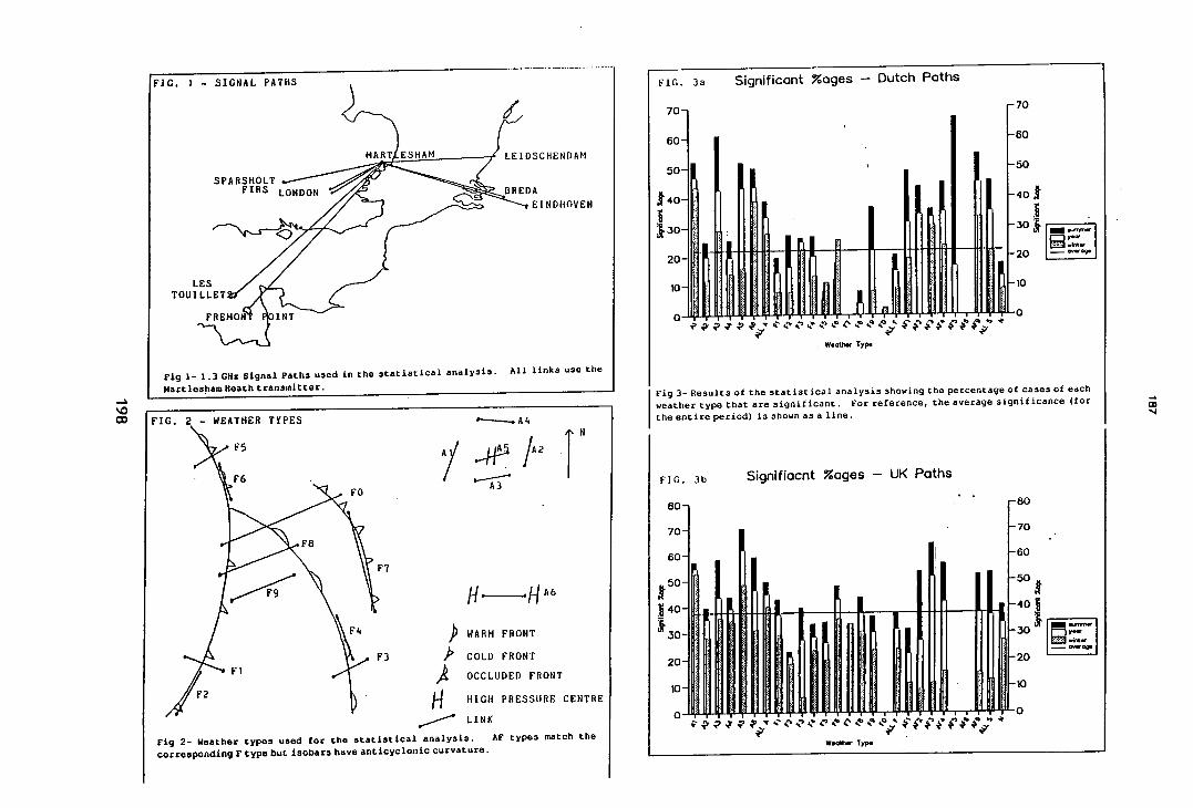
Fl
I I I
-. A 4
V/A21
\ H ./JA6
)F2
F4 WARM FRONT
F3 COLD FRONT h
OCCLUDED FRONT
i-I HIGH PRESSURE CENTRE LINK
Fig 2- Weather types used for the statistical analysis. AF types match the
corresponding F type but isobars have anticyclonic curvature.
\0
I
Li
0
0
O,
I O —d
O — j
FIG. 3a Significant %ages - Dutch Paths
W.oUw Type
Fig 3- Results of the statistical analysis showing the percentage of cases of each weather type that are significant. For reference, the average significance (for the entire period) is shown as a line.
co 1
FIG. 3b Signifiacnt %ages - UK Paths
1 . w.otI_ Tip.
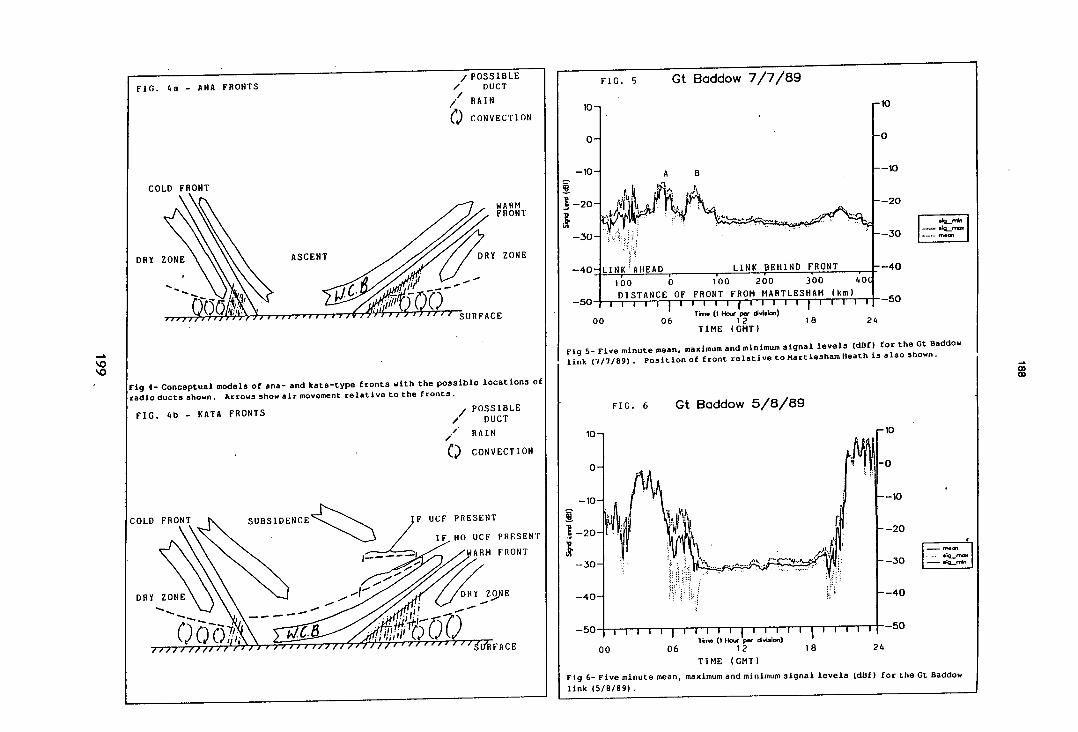
COLD FRONT
DRY ZONE ASCEN
WARM FRONT
DRY ZONE
SURFACE
I
'is - ANA FRONTS / POSSIBLE
DUCT
RAIN
CONVECTION
FIG. 5 Gt Baddow 7/7/89
EL!]
'9
10 f;f
o
—40 - LINK AHEAD LINK BEHIND FRONT --40
100 0 100 200 300 40
DISTANCE OF FRONT FROM MARTLESHAM (km) —50- I I i I i i --50
Ten. (1 .s p viso)
00 06 12 18 2'. TIME (GMT)
Fig 5- Five minute mean, maximum and minimum signal levels (def) for the Gt 8addOW link (7/7/89) - Position of front relative to Hartiesham Heath is also shown.
FIG. 6 Gt Baddow 5/8/89
TIME (GMT)
Fig 6- Five minute mean, maximum and minimum signal levels (def) for the Gt Baddow link (5/8/89).
Fig 4- Conceptual models of ana- and kata-type fronts with the possible locations of radio ducts shown. Arrows show air movement relative to the fronts.
FIG. 'ib - KATA FRONTS / POSSIBLE
/ DUCT
/ RAIN
CONVECTION
COLD FRONT SUBSIDENCE F UCF PRESENT
IF NO IJCF PRESENT
11 ARM FRONT
DRY E
-
F '"FACE
10
20
30
40
50
00

Appendix C
Bibliography
Alexander, F.E.S.
Observations of unorthodox radar vision in the vicinity of New Zealand
and Norfolk Island.
(in Meteorological factors in radio-wave propagation)
The Physical Society, London
Appleton, Sir E.
The influence of tropospheric conditions on ultra-short-wave propagation.
(in Meteorological factors in radio-wave propagation)
The Physical Society, London
Ball, F. K.
Control of inversion height by surface heating.
Q. J. R. Met .Soc. (86)
Barry R.G. & Choi-ley R.J.
Atmosphere, Weather and Climate.
Methuen Co. (5th ed.)
Bean, B.R. & Dutton, E.J.
Radio Meteorology.
(National Bureau of Standards Monograph 92)
U.S. Govt. Printing Office
1947
242-250
1947
1-17
1960
483-494
1987
1966
Ulff
Bennetts, D.A.. Grant, J.R. & McCallum, E. 1988
An introductory review of fronts. Part 1: theory and observations
Met. Maij. 357-70
Bennetts, D.A., Grant, J.R. & McCallurn, E. 1989
An introductory review of fronts. Part II: a case study
Met. May. 8-12
Boithias, L. 1987
Radio wave propagation.
North Oxford Academic Press
Booker, H.G. 1948
Some problems in radio meteorology.
Q. J. R. Met. Soc. (74) 177-215
Booker, H.G. & Walkinshaw, W. 1947
The mode theory of tropospheric refraction and its relation to wave guides.
(in Meteorological factors in radio-wave propagation)
The Physical Society, London 80-127
Browning, K.A & Harrold, T. W. 1969
Air motion and precipitation growth in a. wave depression.
Q. J. R. Met. Soc. 288-309
Browning, K.A & Harrold, T.W. 1970
Air motion and precipitation growth at a cold front.
Q. J. R. Met. Soc. 369-389
Browning, K.A & Pardoe, C.W. 1973
Structure of low-level jet streams ahead of mid-latitude cold fronts.
Q. J. R. Met. Soc. (99) 619-63
Browning, K.A. & Fiji!, F.K. 1981
Orographic Rain.
Weather (36) 326-329
Browning, K.A.(ed) 1982.
Nowcas t lug.
201
Academic Press
Browning, K.A. & Monk, G.A. 1982
A simple model for the synoptic analysis of cold fronts.
Q. J. R. il'iet. Soc. (108) 435-452
Browning, N.A. 1985
Conceptual models of precipitation systems.
Met. iViag. (114) 293-319
Bye, G.D. 1988a
Radio-meteorological aspects of clear air anomalous propagation in NW Europe.
B. Telecom J. Technol. (6) 32-45
Bye, G.D. 1988h
An explanation for the observed statistical results from
the Leidschenda.m—Ei ndlioven 11.7 G I -Iz link.
Unpublished report. copy available from BTL
Bye, G.D. & Howell, R.G. 1989
Average radio refractive index lapse rates in the lower troposphere for locations in NW Europe.
IcAP'SO (lEE CP301) (2) 229-233
CCIR 1986
Recommendations and reports of the CCIR.
XVIth Plenary Assembly. Dubrovnik (V)
Clough, S.A. 1987
The mesoscade frontal dynamics project.
Meteorological Magazine, (116). 32-42
Clough, S.A. & Testud J. 1988
The FRONTS'87 Experiment and Mesoscale Frontal Dynamics Project.
WMO Bulletin (126) 276-281
Clow, D.G. 1984
Weather and microwave radio propagation,
Weather (39) 174-179
202
COST 210 Project 1991
Influence of the atmosphere on interference between radio -
communications systems at frequencies above 1 GlTz.
Commission of the European Communities
DAR 1978
Daily Aerological Record.
H.M.S.O
Diik, J. & van Noort, R. 1989
Statistical results from the links Koeln—Eindhoven (1.3 GHz) and
Leidscheiidam—Eindhoven (11.7 GI -1z).
COST 210 C'tte Paper (139)
Unpublished report, copy available from BTL
DNOM 1984
The effects of the environment on radio and radar wave propagation
(Naval Oceanography and Meteorology Memorandum 1/84).
Directorate of Naval Oceanography and Meteorology,
Dougherty, H.T. & Hart, B.A. 1979
Recent progress in duct propagation prediction.
IEEE Trans. Ant. Prop. (27) 542-548
Durst, C.S. 1947,
Radio climatology.
(in Meteorological factors in radio-wave propagation).
The Physical Society, London 193-211
Flavell, R. G. 1962
The application of potential refractive index in tropospheric wave propagation.
J. Ats. Terr. Phys. (24) 47-56
Flavell, R.G. 1964
Further radio-meteorological analysis using the potential refractive index.
J. Ats. Terr. Phys. (26) 41-49
Flavell, R.G. 1978
Preliminary results of a. six year study of the lower atmosphere over Southern England
203
in terms of RR1 and PRI.
I.E.R.E. Con!. Proc. (40) 265-280
Flavell, R.G. 1981
The use of a dense network of amateur radio stations to determine the limits of
long-range tropospheric propagation within an anticytlone.
IGAP'81 (TEE Conf. Puh.195) 163-167
Flavell, R.G. 1983
Studies of an extensive anticyclonic propagation event and of some short term
enhancements observed at VHF and UHF.
ICAP'83 (TEE Conf. Pub.219) 16-18
Garratt, J.R. 1987
The stably stratified iiitctiiaI boundary layer for steady and diurnally varying offshore flow.
Boundary Layer Meteorology (38) 369-394
Garratt, J.R.. & Ryan, B.F. 1989
The structure of the stably stratified internal boundary layer in offshore foiw over the sea.
Boundary Layer Meteorology (47) 17-40
Gossard, E.E. 1981
Clear weather meteorological effects on propagation at frequencies above 1 GHz.
Radio Science (16)5 589-608
Gossard, E.E. 1982
Formation of elevated refractive layers in the oceanic boundary layer
by modification of land air flowing offshore.
Radio Science (17)2 385-398
Gough, M.W. 1979
UHF signal measurements as a guide to atmospheric structures.
Marconi Review (42)214 135-152
Hall, M.P.M. & Gardiner. G.W. 1968
A psycrometer radiosonde developed for determining radio refractive index
as a function of height.
J. Sci. Inst. (J. Phys. E2) (1) 401-405
204
Hall, M.P.M. k7 Corner. C.M. 1969
Statistics of tropospheric radio refractive index soundings taken over
a 3 year period in the UK.
Proc. lEE (116)5 685-690
Hall, M.P.M. 1979
Effects of the troposphere on radio communications.
Peter Peregrinus Ltd., Stevenage, UK
Hall, M.P.M & Barclay, L.W. (eds) 1989
Radiowave Propagation.
Peter Peregrinu.s Ltd., Stevenage, UK
Hamilton, G.D. & Laevastu, T. 1974
Structures of moisture and temperature profiles in the neat surface layers.
NATO .4.51 on miCrOwave propagation and air-sea interaction 117-129
Hammond, K.P. 1989
Statistical results from the 1.3 GHz North Sea network.
COST 210 C'tte Paper (102)
Unpublished, copy available from BTL.
Hatcher, R.W. & Sawyer. J.S. 1947
Sea breeze structure with particular reference to temperature and
water vapour gradients and associated radio ducts.
Q. J. R. JVIe t. Sc. (73) 391-406
Hewitt. M.T. & Adams. A.R.. 1980
The identification of of trans-horizon interference propagation conditions
from meteorological data.
Post Office Research centre report, unpublished, copy available from BTL
Hewitt. M.T, Adams, Alt & Flavell. R.G 1981
Frontal disturbances in anticyclonic.subsidence a. cause of interference
propagation beyond the horizon.
U.R.S.I General Assembly, Washington D. C.. U.S.A (August 1981)
Hewitt, M.T. 1984
1.3 GHz transhorizon measurements in NW Europe
205
COST 210 C'tte Paper (2)
Unpublished report, copy available from BTL -
Hewitt, M.T. 1985 The use of diurnal patterns in transhorizon propagation research
COST 210 C'tte Paper (35)
Unpublished report, copy available from BTL
Hewitt, M.T. 1987
Clear-air interference propagation characteristics of land, sea and coastal paths in NW Europe
COST 210 C'tte Paper (134)
Unpublished report, copy available from BTL
Hewitt, M.T. 1988a
The BTRL/Yeh "Reference CD" ducting model
COST 210 C'tte Paper (135)
Unpublished report, copy available from BTL
Hewitt, M.T. 1988b
The BTRL/Yeh "Reference CD" troposcatter model
COST 210 C'tte Paper (136)
Unpublished report, copy available from BTL
Hewitt, M.T. 1988c
A new approach to clear-air interference propagation modelling
COST 210 C'tte Paper (234)
Unpublished report, copy available from BTL
HMSO
London Weather Centre Daily Weather Report
HMSO
Hough, M.N.
Forecasting the ducting of radio waves
Met. It/lag.
1986-8
1976
(105) 24-30
Ishimaru, A. 1985
Wave propagation (Chapter 37 of Handbook of applied 'meteorology, Houghton, D.D. (ed)) Wiley
206

Johnson. Sir N. K. 1947
Meteorological investigations hi connection with radio propagation
(in Meteorological factors in radio-wave propagation).
The Physical Society, London 212-5
Jones, T. 1989
An Examination of the BTR.L Anticyclone Model.
Unpublished, copy available at BTL or from the author
Jones, T. 1991
The role of fronts in anomalous microwave propagation.
IGAP'91 (lEE Coif. Pub 333) (1) 185-8
Juy, M. & Spillard, C. 1988
Comparison of meteorological synoptic da.ta with propagation events seen
on paths from France to the UK
COST 210 C'tte Paper (239)
Unpublished report, copy available from BTL
Ko, H.W., Sari, J.W. & Thomas. M.E. 1983
Anomalous propagationand radar coverage through inhornogeneous atmospheres
A CARD ConJi Pub (346)
Kuhn, U. & Ogulewicz, S. 1970
Propagation measurements at 500 MHz over the sea for varying meteorological parameters
Proc. lEE (117)5 879-886
Levy, M.F., Craig, K.H.. Champion, R..J.B., Eastment, J.D. & Whitehead, N1M.
Airborne measurements of anomalous propagation over the English Channel
IGAP'SO (TEE Conf Pub 333) 173-6
Loclitie, G.D. 1985
Transhorizon propagation research: radiation nights
COST 210 C'tte Paper (62)
Unpublished report, copy available front BTL
Machin, N.A. 1988
Fronts 87 Report No 7.
Unpublished memorandum, copy available in National Meteorological Library, Bracknell
207

Mason. Sir J. 1983
Progress in cloud physics and dynamics
Recent advances in meteorology 1-14
Mcllveen, J.F.K. 1986
Basic Meteorology, a physical outline.
Van Nostrand Reinhold
McIntosh, Dii & Thorn, A.S. 1981
Essentials of Meteorology.
Wyke ham
Met.O. 1969
The Observers Handbook.
HMSO
Met.O.
Elementary N'leteoiology.
HMSO
Muihearn, P.J.
On surface-based advective radar ducts
R.A.R.N.L Tech. Note 5/78
Department of Defence (Australia)
Narnias, J.
Subsidence in the atmosphere
Harvard meteorological studies
Nash. J. & Schmidlin, F.J.
'VVMO international radiosonde comparison: final report
W.M. 0. Tech. Doc
Pearson. R..A., Carboni. C. & Brusasca. C.
The sea breeze with mean flow
Q. J. R. Met. Soc.
Rotherha.m, S.
1981
1976
1933
(2)
1987
(195)
1983
(109)
809-30
1974
Propagation theory for the evaporation duct
NATO AS[ Oti microwave propagation, (111(1 air-Sca interaction
Rotherham. S.
Clear air aspects of the troposphere and their effects on
propagation mechanisms from VHF to mm waves
in Hall & Barclay [298.9]
Ryder, P., Lewis A.F. & Bennetts, D.A.
The NAVAID dropsonde.
Mat. Mag. (112)
Sheppard, P. A.
The structure and refractive index of the lower atmosphere
(in Meteorological factors in radio-wave propagation).
The Physical Society, London 37-79
Simpson, J.E., Mansfield, D.A. & Milford. J.R.
Inland penetration of sea-breeze fronts
Q. J. R. Met. Soc. (103)
Smith—Rose, R.L. & Sticklanci, A.C.
An experimental study of the effect of meteorological conditions
upon the propagation of centiinetric radio waves
(in Meteorological factors in radio-wave propagation).
The Physical Society. London 18-37
Spillarci, C.
The dependence of received sign a.! level on meteorological conditions
over the COST 210 cross-Channel links
COST 210 C'tte Paper (323)
Unpublished report, copy available from BTL
164-78
1989
150-72
1983
367-380
1947
1977
47-76
1947
1989a
Spillard, C. 1989b
X-band tropospheric transhorizoii propagation under differing meteorological conditions
IG'AP'SO(lEEConf. Pub 301) (1) 451-6
Spihlard, C. 1991
Transhorizon microwave propagation and its relationship with meteorological conditions
209
Ph.D The.sis, Portsmouth Polytechnic
Stull, R.B. 1988
An introduction to boundary layer meteorology
Kluwer
Thompson, N. 1989
Humidity observations by the Mk 2 & Mk 3 radiosondes and the Vaisala RS8O radiosonde
Met. 0. Tech. Note 56
Unpublished memorandum, COPY available in the National Meteorological Library, Bracknell
Thorpe, A.J. & Clough, S.A. 1991
Mesosca.le dynamics of cold Fronts: Structures described by d ropsoundings in FRONTS '87
Q. J. R. Met. Soc. (117) 903-41
Turton, J.D., Bennetts, D.A. & Farmer, S.F.G.
An introduction to radio ducting
iVie t. Mag. (117)
Weston.K.J.
Bringing the analysis of occluded fronts into the satellite age.
Met. Mag (116)
0.
'f- r/ iø
?
4)
1988
245-254
1987
19-21
/9J0
z9 7-309
210


