Comparison between Met Office and ECMWF medium-range ensemble forecast systems Authors: Helen Titley, Nicholas Savage, Richard Swinbank and Simon Thompson
Date Version Action/comments: Approval
12/3/07 1.1 Combine draft sections .
3/4/07 1.2 Amended and issued as project report R. Swinbank
7/8/07 1.3 Update case studies
4/1/08 1.4 New section with objective verification; other miscellaneous changes
11/1/08 1.5 Further amendments for issue as Met R&D tech report
17/1/08 1.5 Approved for issue as technical report A.C. Lorenc
26/2/08 1.5 Correct report number to 512 from 507
Last printed – 26/02/08
Comparison between Met Office and ECMWF medium-range ensemble forecast systems
Helen Titley, Nicholas Savage, Richard Swinbank and Simon Thompson
Summary This report compares several aspects of the Met Office and ECMWF medium-range ensemble prediction systems. We compare three major aspects of the performance of the ensemble forecasts: Systematic errors: Based on a set of 20 hindcasts (10 summer and 10 winter), it is shown that the systematic model errors are comparable in the two systems. In some instances, the Met Office biases were smaller; in other examples, the ECMWF biases were smaller. Overall, the ECMWF model generally had the edge. Prediction of high-impact weather: Since high-impact events are relatively rare, it is rather limiting to compare the performance of ensemble forecasts using objective statistics alone. Using a set of case studies of forecasts of high-impact weather events, it was found that there were some aspects where the guidance from MOGREPS-15 was better, and other cases where ECMWF gave a better indication of high-impact weather. Objective statistics: To complement the case studies, we have also considered objective verification statistics using forecasts from 1 January 2007 to 15 November 2007. A range of different statistics has been calculated using the area-based verification (VER) system. Both statistics based on the ensemble means and probabilistic verification statistics indicate that the ECMWF ensemble generally performs better than MOGREPS-15. The overall conclusion is that the Met Office medium-range performance does not quite match the performance of the ECMWF. However, there were many aspects of the Met Office performance that were competitive with ECMWF. This indicates scope for a multi-model ensemble to pick up the most skilful aspects of each of the component forecasts. It is encouraging that MOGREPS-15 is competitive despite the difference in development times of the two ensembles.
1. Introduction The main focus of the Met Office THORPEX research project is the evaluation of the benefit of a possible future multi-model medium-range ensemble forecast system. That multi-model ensemble forecast would entail the combination of ensemble forecasts from a Met Office with ensembles from other forecast centres. This forms part of the international THORPEX Interactive Grand Global Ensemble (TIGGE) project. As a step towards that goal, this paper evaluates the quality of the Met Office medium-range ensemble forecasts (designated MOGREPS-15) by comparing them with equivalent results from the ECMWF ensemble prediction system (EPS). Experiments with earlier versions of the Met Office and ECMWF models demonstrated the potential benefits to medium-range forecasting from the combination of ensemble forecasts from both models (Harrison et al, 1995). More recently, the DEMETER project (Palmer et al, 2004) demonstrated the benefit of combining ensembles forecasts from several models for seasonal forecasting. Hagedorn et al (2005) showed that that, the DEMETER models had different strengths and weaknesses, so the multi-model results were an improvement over each of the component ensembles. Nevertheless, to get the most benefit from a possible future multi-model ensemble system, it is important that the component models each add some skill to the combination. Thus, we need to ensure that the MOGREPS-15 is competitive with other ensemble systems contributing to TIGGE. The ECMWF EPS is one of the leading operational global ensemble prediction systems; a comparison of the MOGREPS-15 and
1
ECMWF ensembles will give a good indication of how the experimental MOGREPS-15 forecasts compare with other likely contributors to a future multi-model ensemble. In section 2, we give an overview of the two ensemble systems. Section 3 compares the systematic errors in the ensembles forecast models, using a set of 20 case study forecasts. A key emphasis of THORPEX is the improvement in the forecasting of high-impact weather. Section 4 compares the performance of the ensemble forecasts in several case studies centred on high-impact weather events. To complement these results, some objective comparisons of the ensembles are presented in section 5, based on results from the area-based verification package (VER). The overall results are summarised in section 6.
2
2 Overview of Ensemble Forecast Systems Met Office (MOGREPS) The Met Office ensemble forecasts are run using a global configuration of the Met Office Global and Regional Ensemble Prediction System (MOGREPS) (Bowler et al, 2007a,b). The system was originally developed for short-range ensemble forecasts over the UK. Boundary conditions for the regional ensembles forecasts are provided by running global short-range ensemble forecasts. For the THORPEX research project, the forecast component of MOGREPS was ported to run on the ECMWF supercomputer, and the range of the forecasts was extended to 15 days (hence MOGREPS-15). Each ensemble forecast is run with 24 members: one control run and 23 members with perturbations. The initial conditions for the control run are interpolated from the operational 4D-Var global data assimilation system (Rawlins et al, 2007). Perturbations are calculated using an Ensemble Transform Kalman Filter (Bishop et al, 2001) and added to the control data to produce initial conditions for the perturbation runs. The forecast model uses a resolution of N144 (i.e. 0.83° latitude by 1.25°longitude) with 38 levels. The version of the model used for the early results presented in this report used a set of physical parameterizations denoted “HadGEMminus” (Milton et al, 2007), i.e. close to what was used for the HadGEM1 climate model (Martin et al, 2005). From 0Z on 13th June 2007, the MOGREPS-15 system was updated to use the set of parameterizations adopted for the operational global forecast model in spring 2006 (model cycle G39, also denoted PS11, for Parallel Suite 11), see Savage et al (2007). The comparison of systematic model errors (section 3) is based on the PS11 physics. The case studies (section 4) and objective verification statistics (section 5) are based on a mixture of HadGEMminus and PS11 model versions. The perturbation forecast runs also include two stochastic physics schemes: Random parameters and Stochastic Convective Vorticity (Bowler et al, 2007a).
ECMWF EPS The ECMWF has been running an operational ensemble prediction system since December 1992 (Molteni et al, 1996). For most of the period covered by this study, the ECMWF EPS used a model resolution of TL399L62 (spectral triangular truncation T399 with a linear grid, and 62 levels), and the forecast range was 10 days. Since 12th September 2006, the system has been run with variable resolution: TL399L62 out to day 10, and a TL255L62 resolution between days 10 and 15. This variable-resolution system is known as VAREPS (Buizza et al, 2007). For some of the cases used for the comparisons of systematic errors (before February 2006), the ECMWF EPS resolution was TL255L40. The ECMWF EPS is run with 51 members: one control run and 50 perturbed runs. The initial condition perturbations are based on the singular vector method (Buizza and Palmer, 1995). The perturbations are based on the modes that grow most rapidly during the first 48 hours of the forecast, calculated at resolution T42L62. The ECMWF system also includes stochastic physics schemes to take account of uncertainties in the model parameterizations (Buizza et al, 1999).
3
3 Comparison of systematic errors between Unified Model and control of ECMWF EPS system.
In order to gain an understanding of the biases of the MOGREPS-15 forecasts, the systematic errors have been compared with result from control runs of the ECMWF EPS. The MOGREPS-15 results are taken from the 20 cases used to evaluate the new PS11 physics changes (Savage et al, 2007). The 20 cases (10 winter cases and 10 summer cases) are tabulated in Table 3.1. The results here compare the (deterministic) forecasts using the PS11 physics with the ECMWF control forecasts for the corresponding dates. Although the ECMWF EPS was normally run for 10 days, the control forecasts were all run out to 21 days for the period of interest. Note that the ECMWF EPS resolution was T255 until 22nd February 2006 (all winter cases, and the first 5 summer cases) and T399 thereafter. The ECMWF fields were all re-gridded to N144 resolution for this comparison.
Table 3.1: Initial analysis dates (12 UTC) for the case study forecasts
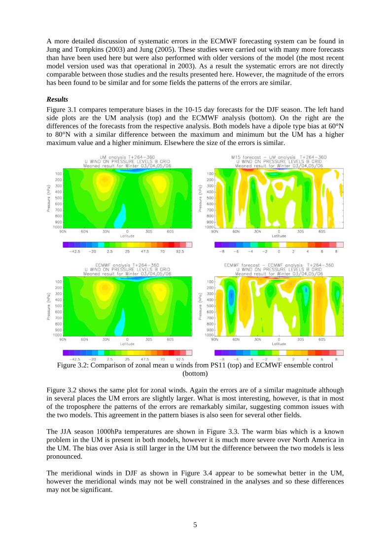
Figure 3.1: Comparison of zonal-mean temperature from PS11 (top) and ECMWF ensemble control (bottom)
4
A more detailed discussion of systematic errors in the ECMWF forecasting system can be found in Jung and Tompkins (2003) and Jung (2005). These studies were carried out with many more forecasts than have been used here but were also performed with older versions of the model (the most recent model version used was that operational in 2003). As a result the systematic errors are not directly comparable between those studies and the results presented here. However, the magnitude of the errors has been found to be similar and for some fields the patterns of the errors are similar. Results Figure 3.1 compares temperature biases in the 10-15 day forecasts for the DJF season. The left hand side plots are the UM analysis (top) and the ECMWF analysis (bottom). On the right are the differences of the forecasts from the respective analysis. Both models have a dipole type bias at 60°N to 80°N with a similar difference between the maximum and minimum but the UM has a higher maximum value and a higher minimum. Elsewhere the size of the errors is similar.
Figure 3.2: Comparison of zonal mean u winds from PS11 (top) and ECMWF ensemble control
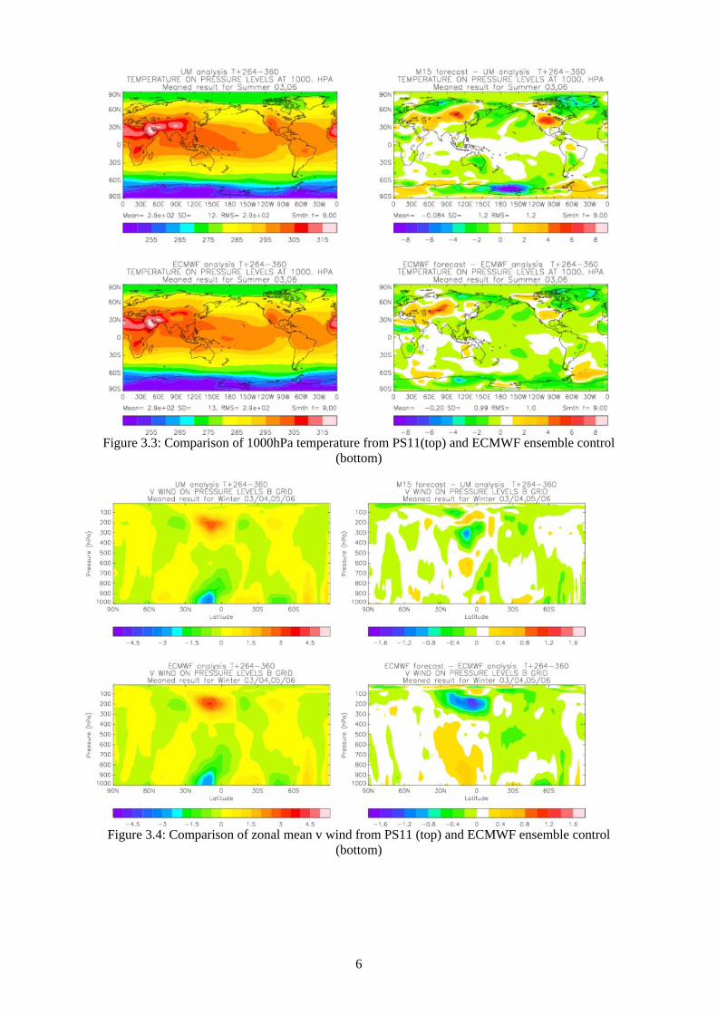
(bottom) Figure 3.2 shows the same plot for zonal winds. Again the errors are of a similar magnitude although in several places the UM errors are slightly larger. What is most interesting, however, is that in most of the troposphere the patterns of the errors are remarkably similar, suggesting common issues with the two models. This agreement in the pattern biases is also seen for several other fields. The JJA season 1000hPa temperatures are shown in Figure 3.3. The warm bias which is a known problem in the UM is present in both models, however it is much more severe over North America in the UM. The bias over Asia is still larger in the UM but the difference between the two models is less pronounced. The meridional winds in DJF as shown in Figure 3.4 appear to be somewhat better in the UM, however the meridional winds may not be well constrained in the analyses and so these differences may not be significant.
5
Figure 3.3: Comparison of 1000hPa temperature from PS11(top) and ECMWF ensemble control
(bottom)
Figure 3.4: Comparison of zonal mean v wind from PS11 (top) and ECMWF ensemble control
(bottom)
6
Figure 3.5: Comparison of zonal mean RH from PS11 (top) and ECMWF ensemble control (bottom)
Finally, Figure 3.5 shows the zonal mean of relative humidity for JJA. The main source of differences in the analyses is the different definitions of relative humidity used. In the ECMWF results RH is defined with respect to water above 273.16 K, to ice below 250.16 K, and with respect to a mixture of both in between while the Unified model uses RH with respect to water everywhere. The forecasts also have very different error fields with a moist bias at 100hPa in the UM, and a dry bias below, while in the ECMWF model there is a dry bias at 100hPa and a moist bias below. Conclusions Some systematic errors of the Unified Model results are similar to those of the ECMWF ensemble control, for other errors the UM is significantly worse and for some errors the Unified model may be slightly better. Overall these results are very encouraging, giving confidence in the performance of the MOGREPS system relative to ECMWF at least as far as issues related to biases are concerned. Although there are clear areas where improvements can be made, the results suggest that the version of the system based on PS11 can provide a useful basis for forecasting out to 15 days. A further upgrade to the model physical parameterizations was implemented from 0Z on 27th November 2007. These changes were designed to address many of the issues discussed above, particularly the summer warm bias. For further information, see Savage (2007).
7
4. Case studies of high-impact weather 4.1 Case Study 1: 18 January 2007 – Strong winds over the UK
Description of weather event
A vigorous depression passes across the UK bringing severe gale-force winds over England, Wales and Northern Ireland, with widespread gusts of 70-80 mph, including 77mph at Heathrow (2mph higher than in 1987 storm). A top gust of 99mph was experienced on the Isle of Wight. This is the strongest storm to hit such a large area of the UK since 1990. The storm goes on to give gusts up to 124mph across the Netherlands, Germany and Poland.
Figure 4.1.1: MSLP Analysis at 12Z 18/01/07
Figure 4.1.2: MOGREPS-15 control analysis for 12 UTC 18/01/2007, showing contours of mean sea
level pressure. Red areas indicate a) surface winds >34kt and b) 925mb winds > 60 kt The initial frontal wave forms along the strong thermal gradient over the US, becoming an enclosed low of 1010mb over Lake Erie at 12Z on 15th January. The depression propagates and deepens within the Westerly flow of the strengthening upper jet, and at 00Z 17th is a low of 982mb east of Newfoundland. Eighteen hours later the low has deepened further to 962, but by 00Z 18th the low has become elongated and started to split into two. It is the newly developing eastern flank of the low that continues to develop and advance rapidly across the UK, entering the North Sea by 12Z 18th. The low deepens as it passes over mainland Europe, before slowing and gradually filling. Impact The storm led to 11 deaths in the UK and 43 across Northern Europe. There was a loss of power in 10,000s of homes, and structural damage to many properties. Part of the roof was blown off from Lord's Cricket ground. The container shop MSC Napoli was stranded in the English Channel, with 26 crew airlifted to safety. Deterministic model performance (from Adrian Semple’s daily weather summary (Semple, 2007)) Although somewhat erratic at the longer ranges concerning the precise position and depth of the vigorous depression crossing the UK during today, the Global Model generally showed a good and consistent signal for the storm at the verification time (12z 18th). Even at T+132, the surface pressure is only 1hPa too low. The two subsequent forecasts show a decrease in skill, but the T+96 solution provides good guidance once again of a deep low with strong gradient on its southern flank. From T+72, the forecasts show a consistent scenario with small positional errors, a strong pressure gradient and depth errors generally 1-5hPa.
8
The Global Model performance is generally better than that of the ECMWF deterministic model, with errors consistently larger in the ECMWF fields than in the Global. Of particular note are the T+24 to T+48 short range forecasts in which the ECMWF 500hPa trough is shown to be far too diffluent with respect to the analysis. That of the Global Model is significantly better, with smaller errors. The impact of this in the MSLP surface is that the field shows a significantly better depth and position for the low over the North Sea. This general trend extends into the longer range, e.g. at T+84 when the ECMWF model suffers a significant forecast bust, with the low forecast to be to the south of Iceland. The Global Model, however, maintains a deep depression in the North Atlantic at this range. Comparison of Met Office and ECMWF EPS Surface winds
Figure 4.1.3: MOGREPS-15: probability of surface winds > 34 knots at VT 12Z 18/01/2007 Figure 4.1.3 shows the forecast probability of surface winds greater than 34 knots for lead times of 1, 2, 3, 4, 6, 8, 11 and 14 days using the Met Office 15-day ensemble. For reference Figure 4.1.2a shows where surface winds were greater than 34 knots in the control analysis. At T+24 between 75% and 100% of members are forecasting gale-force winds over a large part of the affected area.. At T+48 there is a dip in the forecast probability, but by T+72 the ensemble returns to forecasting greater than 75% probability over the areas of the North Sea and to the West of Ireland, with between 25% and 75% probability in the other areas shown in the analysis. Similar patterns are shown and T+96, and T+144, with most of the key areas still showing between 25 and 75% probability of gale-force winds at a 6-day lead time. At T+192 (8 days ahead), the ensemble is still showing a risk of gales all around the UK but the location specificity has lessened. In the ensemble mean of mean sea level pressure (overlaid in contours) by this time the low is too far to the north and west. For lead times of 10+ days the ensemble spread is such that no clear signal for gales, with the risk greater than 25% only out to the west of the UK.
Figure 4.1.4: ECMWF EPS ensemble: probability of surface winds > 34 knots at VT 12Z 18/01/2007
9
Figure 4.1.4 shows the same probability maps of gale-force winds but for the ECMWF EPS. At 24-hour and 48-hour lead times the overall pattern is similar to MOGREPS-15, although the ensemble mean mslp has the low positioned too far north and west. At T+72 the ensemble is forecasting a larger risk of gales in the Channel and over the UK land mass, but a smaller risk in other areas when compared to MOGREPS-15. The very strong wind speeds in the North Sea at the validity time are forecast with a lower probability in the ECMWF EPS compared to MOGREPS at T+96 and T+144. At lead times of T+192 and greater the patterns are similar in both ensembles, although ECMWF continue to forecast a hint of gales over the UK land mass. 925mb winds
Figure 4.1.5: MOGREPS-15: probability of 925mb winds > 60 knots at VT 12Z 18/01/2007
Figure 4.1.6: ECMWF EPS ensemble: probability of 925mb winds > 60 knots at VT 12Z 18/01/2007 Figures 4.1.5 and 4.1.6 show the forecast probability of 925mb winds greater than 60 knots for MOGREPS-15 and the ECMWF EPS respectively. This approximates to the traditional “level 6 wind” diagnostics used by forecasters to estimate surface gust speed. Higher probabilities of gusts greater than 60 knots in the affected areas (see Figure 4.1.2b for reference) are given by MOGREPS out to T+192. There is a strong indication (>75% probability) out to T+120 for high potential gust speeds in the key area to the south of the low. The signal begins to dampen at T+144 and T+192 but is still stronger in MOGREPS-15 than the ECMWF EPS. At lead times of 10 days or more there is no clear signal in either ensemble. Example postage stamps Figures 4.1.7 and 4.1.8 show example postage stamps (in this case from T+120) valid at the peak of the storm for the UK for MOGREPS-15 and the ECMWF EPS respectively. Both have members showing the correct solution, and the majority of members show a low present somewhere, with very high gradients of PMSL present over the UK. There is uncertainty in the timing and track of the low, but when combined together the two models show good support for a severe weather event over the
10
UK. A greater proportion of members in MOGREPS-15 have the low correctly positioned in the North Sea.
Figure 4.1.7: T+120 MOGREPS-15 postage stamps of PMSL for VT 12Z 18/01/2007
Figure 4.1.8: T+120 ECMWF EPS postage stamps of PMSL for VT 12Z 18/01/2007
At longer lead times than this the uncertainty over the timing and the track of the low increases, and the traditional charts (e.g. postage stamps and probability charts of high winds in a particular location at a particular time) start to show this apparent loss of signal in the ensemble. However, although the detail of the situation becomes more uncertain at longer lead times, ensemble forecasts can still provide useful guidance of the broader risk of a storm affecting some part of the UK within a set
11
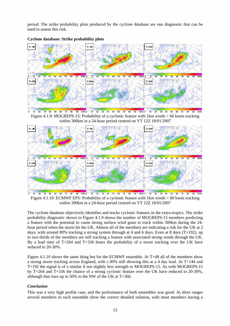
period. The strike probability plots produced by the cyclone database are one diagnostic that can be used to assess this risk. Cyclone database: Strike probability plots
Figure 4.1.9: MOGREPS-15: Probability of a cyclonic feature with 1km winds > 60 knots tracking
within 300km in a 24-hour period centred on VT 12Z 18/01/2007
Figure 4.1.10: ECMWF EPS: Probability of a cyclonic feature with 1km winds > 60 knots tracking
within 300km in a 24-hour period centred on VT 12Z 18/01/2007 The cyclone database objectively identifies and tracks cyclonic features in the extra-tropics. The strike probability diagnostic shown in Figure 4.1.9 shows the number of MOGREPS-15 members predicting a feature with the potential to cause strong surface wind gusts to track within 300km during the 24-hour period when the storm hit the UK. Almost all of the members are indicating a risk for the UK at 2 days, with around 80% tracking a strong system through at 4 and 6 days. Even at 8 days (T+192), up to two-thirds of the members are still tracking a feature with associated strong winds through the UK. By a lead time of T+264 and T+336 hours the probability of a storm tracking over the UK have reduced to 20-30%. Figure 4.1.10 shows the same thing but for the ECMWF ensemble. At T+48 all of the members show a strong storm tracking across England, with c.90% still showing this at a 4 day lead. At T+144 and T+192 the signal is of a similar if not slightly less strength to MOGREPS-15. As with MOGREPS-15 by T+264 and T+336 the chance of a strong cyclonic feature over the UK have reduced to 20-30%, although that rises up to 50% to the NW of the UK at T+366. Conclusion This was a very high profile case, and the performance of both ensembles was good. At short ranges several members in each ensemble show the correct detailed solution, with most members having a
12
strong gradient over the UK. Even at a lead time of 8 days, over half of the ECMWF ensemble, and up to 70% of the Met Office 15-day ensemble members were showing a cyclonic feature with potential for gusts greater than 60 knots passing over the UK on 18th January. There is no doubt that having access to both ensembles, that in this case were both showing a good signal for a strong storm over the UK, would have added extra confidence to the excellent advance warnings that were given for this high-impact event. 4.2 Case Study 2: 31 December 2006 – New Years’ Eve gales over the UK Description of weather event On New Year’s Eve, an intense extra-tropical cyclone passed over Scotland giving gale-force winds over Northern Ireland, southern Scotland, and Northern England. The highest wind gust was near 100mph at Great Dunn Fell (Cumbria). The system developed as a frontal wave in the mid-Atlantic on the evening of 29th December, and developed rapidly to become an enclosed low of 986mb by 00Z on 31st. Twelve hours later (12Z 31st, Figure 4.2.1) it had deepened to 972, before bottoming out at 969mb and slowly filling over the North Sea on 1st January.
Figure 4.2.1: Cyclone database analysis at
12Z 31/12/06
Figure 4.2.2: Area with 925mb winds > 60kt
in MOGREPS-15 control analysis at 12Z 31/12/2006
Impact The storm was very high profile due to its occurrence on New Year’s Eve. Several large events were cancelled including Hogmanay in Edinburgh and Glasgow, firework parties in Liverpool and Newcastle, and an outside concert in Belfast. The storm led to loss of power in 1000s of homes across Northern Ireland, Scotland and Northern England, with structural damage to many properties. In Cornwall a man died when he was swept into the sea from rocks at Trevone Bay, near Padstow in gales and high seas. Cyclone Database: Feature-specific tracks and plumes As mentioned above, the storm that affected the UK on New Years’ Eve was a rapidly developing feature, which only appeared on ASXX (analysis) charts as an enclosed low at 00Z 31/12/2006. Many traditional cyclone identification and tracking methods require a low pressure minima and so would have been very late in identifying this storm. The Cyclone Database uses alternative objective techniques that relate closely to conceptual models of cyclone development to identify and track cyclonic features. The key feature in this case first appeared in the cyclone database analysis at 00Z 30/12/06 as a frontal wave in the mid-Atlantic (Figure 4.2.3a), 24 hours prior to it becoming an enclosed low. 12 hours later the associated trough had begun to deepen and the feature was developing rapidly (Figure 4.2.3b). At these short forecast ranges, interactive clickable maps allow the user to select a feature in the control analysis, bringing up feature-specific plumes of intensity measures with coincident maps of the tracks forecast by each ensemble
13
members. These feature-specific products also provide a valuable tool for comparing the performance of the two ensembles in this case at the shorter range.
Figure 4.2.3a: Analysis at 00Z 30/12/06.
Frontal wave has developed at c.39N,45W.
Figure 4.2.3b: Analysis at 12Z 30/12/06.
Trough associated with wave (42N,34W) has sharpened.
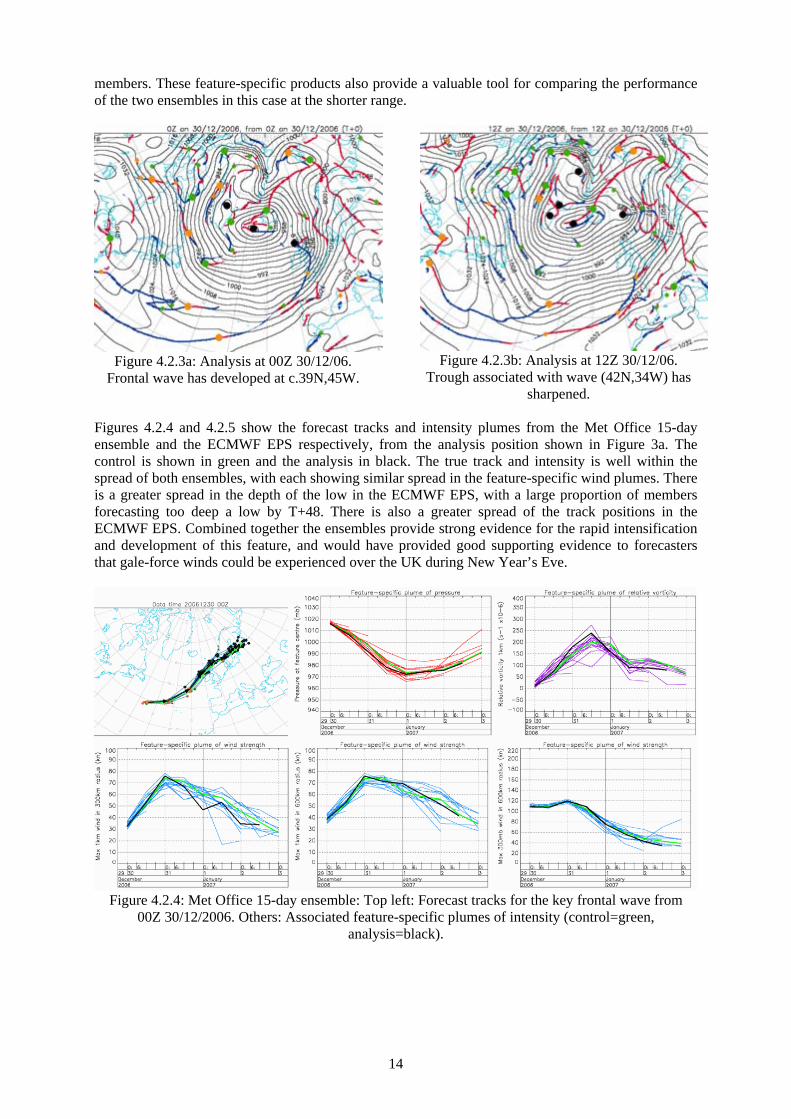
Figures 4.2.4 and 4.2.5 show the forecast tracks and intensity plumes from the Met Office 15-day ensemble and the ECMWF EPS respectively, from the analysis position shown in Figure 3a. The control is shown in green and the analysis in black. The true track and intensity is well within the spread of both ensembles, with each showing similar spread in the feature-specific wind plumes. There is a greater spread in the depth of the low in the ECMWF EPS, with a large proportion of members forecasting too deep a low by T+48. There is also a greater spread of the track positions in the ECMWF EPS. Combined together the ensembles provide strong evidence for the rapid intensification and development of this feature, and would have provided good supporting evidence to forecasters that gale-force winds could be experienced over the UK during New Year’s Eve.
Figure 4.2.4: Met Office 15-day ensemble: Top left: Forecast tracks for the key frontal wave from
00Z 30/12/2006. Others: Associated feature-specific plumes of intensity (control=green, analysis=black).
14
Figure 4.2.5: ECMWF EPS: Top left: Forecast tracks for the key frontal wave from DT 00Z 30/12/2006. Others: Associated feature-specific plumes of intensity (control=green, analysis=black). Figures 4.2.6 and 4.2.7 show the same products 12-hours later, from the analysis position shown in Figure 4.2.3b. Again the analysis track and intensity is well within the spread of both ensembles. Both control forecasts are very close to the analysis in the pressure plume, but the control underestimates the maximum 1km wind speed within the low’s circulation, which sits amongst the most extreme members in both ensembles, particularly the ECMWF EPS. There is greater initial spread in the wind strength in MOGREPS-15. Both models show that little uncertainty in the track of the feature, giving added confidence to the forecasts to customers of where the strongest winds would occur.
Figure 4.2.6: Met Office 15-day ensemble: Top left: Forecast tracks for the key frontal wave from
12Z 30/12/2006. Others: Associated feature-specific plumes of intensity (control=green, analysis=black).
15
Figure 4.2.7: ECMWF EPS: Top left: Forecast tracks for the key frontal wave from DT 12Z
30/12/2006. Others: Associated feature-specific plumes of intensity (control=green, analysis=black). Cyclone database: Strike probability plots
Figure 4.2.8: Met Office 15-day ensemble: Probability of a cyclonic feature with 1km winds > 60
knots tracking within 300km in a 24-hour period centred on VT 12Z 31/12/2006
Figure 4.2.9: ECMWF EPS: Probability of a cyclonic feature with 1km winds > 60 knots tracking
within 300km in a 24-hour period centred on VT 12Z 31/12/2006
16
The strike probability diagnostic shown in Figure 4.2.8 shows the number of MOGREPS-15 members predicting a feature with the potential to cause surface wind gusts > 60 knots to track within 300km during the 24-hour period when the storm hit the UK. Almost all of the members are indicating a risk for the northern half of the UK at 2 days, with around 80% tracking a strong system through at 4 days. By 6 days half of the members are still tracking a feature with strong gust potential across the UK. By week two (the bottom three images), only 30-40% of members track a strong feature through during the verification period. Figure 4.2.9 shows the same thing but for the ECMWF ensemble. At T+48 and T+96 a similar risk is shown to the MOGREPS-15 ensemble. At T+144 up to 60% of members indicate a risk of a strong storm, but by week two a smaller percentage (10-20%) of the ECMWF EPS point towards a cyclone with strong 1km winds tracking over the north of the UK compared to MOGREPS-15. Conclusion This storm was of a particularly high-impact for its intensity because it fell on New Year’s Eve, and led to the cancellation of several high-profile events. The performance of both ensembles was good in week one. At short ranges the spread was relatively low, particularly in the tracks of the Met Office ensemble, with the true solution still falling well within the spread. At a six day lead time between 50-60% of members indicate a risk of a strong storm over the UK. In week two there is not a strong signal in either ensemble for a storm striking the UK, although it is slightly stronger in the Met Office than in the ECMWF EPS. 4.3 Case Study 3: Snow event 8-9 February 2007 Description of weather event A cold air mass had become stagnant over the UK over the previous days. Overnight into 8th February a frontal system pushed in from the SW, with a band of heavy frontal rain associated with the occluded front (see Figure 4.3.1a). As the frontal system advanced NE the precipitation fell through increasingly colder air, and readily turned to snow. The advance north of the band stalled over a broad area of Wales and central and Southern England resulting in significant snow accumulations, with 3-8cm common, and up to 15cm in localised areas. Overnight into 9th February a depression drifted up from the SW approaches (See Figure 4.3.1b). The front on its forward flank was associated with a band of very heavy rain which spread across Devon, Cornwall and south Wales by dawn. The precipitation initially fell through the milder air entrained within it, but as it pushed into the southwest Midlands during the morning, this increasingly fell through much colder air, causing freezing rain at the leading edge of the rain band, and turning to heavy snow to the rear. The broad area of heavy snow moved north during the afternoon across Wales and central England as the shallow depression drifted along the south coast. 2-8cm of additional accumulation results in the Midlands with up to 15cm extra on the higher ground of Wales.
Figure 4.3.1a: ASXX chart for 12Z 08/02/07
Figure 4.3.1b: ASXX chart for 12Z 09/02/07
17
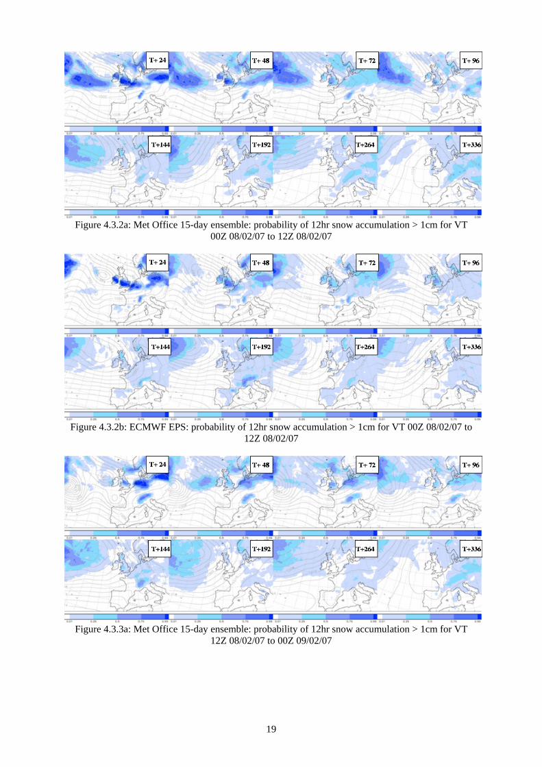
Impact On Thursday 8th the runways at Gatwick, Stansted, Birmingham, London City, Cardiff, Bristol, Luton and Norwich airports were closed for a time and some short-haul British Airways flights from Heathrow and Gatwick airports were cancelled. On the railways, Virgin Trains, First Great Western, Midland Mainline, and South West Trains services were disrupted. All schools in Birmingham, Dudley and Worcestershire were closed on Thursday and Friday. On the evening of Friday 9th roads became gridlocked across the West Midlands as commuters tried to head home. Birmingham city centre was at a standstill and more than 15 miles of queuing traffic was stuck on the M5, between J4 and the M6 link, when the evening rush hour started early. About 250 cars were abandoned between Hereford and Worcester on the A4103 and traffic was at a standstill in Malvern, Worcestershire, because of jack-knifed lorries. On public transport Arriva Midlands suspended bus services in Shrewsbury and Telford and Central trains reported delays between Birmingham and Hereford after a lorry hit a bridge near Hereford. About 2,000 people across Herefordshire and Worcestershire were left without power. Deterministic model performance (from Adrian Semple’s daily weather summary (Semple, 2007)) 8th February: The Global Model verified well in forecasting the low to the W of the UK with a good representation of the SE extension towards the UK that was responsible for the proximity of the front to the colder airmass over the north of the UK. Even at T+144 the solution described the scenario. Earlier forecasts show some considerable scatter in depth and position, although this was insufficient to cause significant departure from the overall consensus of solutions. 9th February: The Global Model fails to accurately represent the snow-bearing depression moving up from the SW approaches until the very short-range. The verifying forecasts show large variation throughout the forecast ranges across the UK and Europe, with the first development of the low occurring in the 00Z 7th T+48 forecast. Development of the system is only a partial success however, as the forecast tracked the system across southern France, giving no snow risk over the UK. Even the 00Z 8th T+24 forecast fails because the forecast track of the system is across northern France. Only the 00Z 9th T+12 (VT 12z 9th) run can therefore be judged as truly successful as it correctly predicted a northward curve to the depression bringing it over the UK. The Global Model therefore provided less than 24 hours warning of threat of heavy snow. Situations such as this however, are not unexpected when small perturbations along a strong jet may develop rapidly. In such a case predictability and resolution considerations are expected to be high. A comparison of the Global Model and ECMWF deterministic model (~25km 91L) at 12z 9th shows that the EC's first development of the low occurs at the 00z 7th T+60 forecast, which is therefore the same run as that of the Global Model. The track of the EC solution is far superior to that of the Global Model however, with the EC track running through the English Channel whilst that of the Global Model ran through Biscay. The EC maintains/improves the track with subsequent runs, bringing the system across the UK on the correct north-easterly track, although solutions vary greatly from run to run in the forecast depth of the low. The 12z 8th EC run achieves a solution in which the developed low both possesses a closed centre and a track into SW UK. This is the earliest model run to achieve this and is 12 hours ahead of the Global Model. The EC deterministic model is therefore judged as providing generally better guidance than that of the Global Model from T+60. Comparison of Met Office and ECMWF EPS Snow probability charts Figures 4.3.2-4.3.4 show the forecast probability of greater than 1cm of snow in 12 hours at each point from the Met Office 15-day ensemble (a) and ECMWF EPS (b), for lead times of 1, 2, 3, 4, 6, 8, 11 and 14 days. Figure 4.3.2 shows the forecast probabilities for the morning of Thursday 8th February, when the snow affected much of Wales and the Midlands. The two ensembles show very similar patterns, each showing high probabilities in the correct area out to a four-day lead time (T+96). At T+144 and T+192 there is still a small signal for snow in the ensemble, but at T+264 and T+366 neither ensemble shows a risk of snow in the correct area.
18
Figure 4.3.2a: Met Office 15-day ensemble: probability of 12hr snow accumulation > 1cm for VT
00Z 08/02/07 to 12Z 08/02/07
Figure 4.3.2b: ECMWF EPS: probability of 12hr snow accumulation > 1cm for VT 00Z 08/02/07 to
12Z 08/02/07
Figure 4.3.3a: Met Office 15-day ensemble: probability of 12hr snow accumulation > 1cm for VT
12Z 08/02/07 to 00Z 09/02/07
19
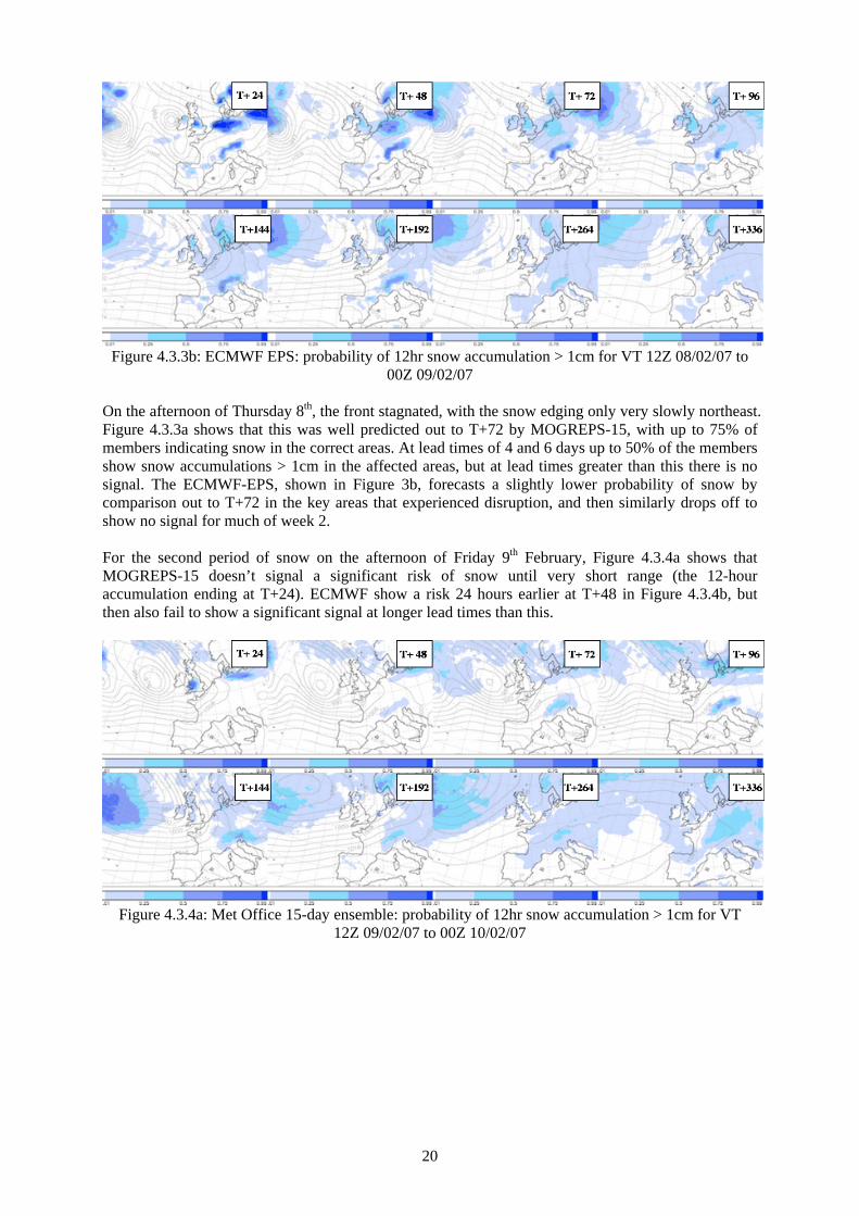
Figure 4.3.3b: ECMWF EPS: probability of 12hr snow accumulation > 1cm for VT 12Z 08/02/07 to
00Z 09/02/07 On the afternoon of Thursday 8th, the front stagnated, with the snow edging only very slowly northeast. Figure 4.3.3a shows that this was well predicted out to T+72 by MOGREPS-15, with up to 75% of members indicating snow in the correct areas. At lead times of 4 and 6 days up to 50% of the members show snow accumulations > 1cm in the affected areas, but at lead times greater than this there is no signal. The ECMWF-EPS, shown in Figure 3b, forecasts a slightly lower probability of snow by comparison out to T+72 in the key areas that experienced disruption, and then similarly drops off to show no signal for much of week 2. For the second period of snow on the afternoon of Friday 9th February, Figure 4.3.4a shows that MOGREPS-15 doesn’t signal a significant risk of snow until very short range (the 12-hour accumulation ending at T+24). ECMWF show a risk 24 hours earlier at T+48 in Figure 4.3.4b, but then also fail to show a significant signal at longer lead times than this.
Figure 4.3.4a: Met Office 15-day ensemble: probability of 12hr snow accumulation > 1cm for VT
12Z 09/02/07 to 00Z 10/02/07
20
Figure 4.3.4b: ECMWF EPS: probability of 12hr snow accumulation > 1cm for VT 12Z 09/02/07 to
00Z 10/02/07 The reason for this difference in performance between the ensembles was examined by consulting the postage stamps. No member of the MOGREPS Global ensemble successfully represented the low's development at the T+36 range, with 6/24 members doing so at the T+24 range. However, only 2 members show an improved solution over the deterministic model with a closed low. The track of the depression in these members remains too far south to provide good forecast guidance for the snow event over the UK. The ECMWF ensemble begins to indicate a low level probability (~10%) of the correct storm development at 00z 6th T+72 with a low to the W of the UK and a small low moving NE from Biscay. This gradually increases to ~50% in the 00z 7th T+48 run. In the 00z 7th T+60 ensemble forecast it is estimated that ~30% of the members indicate a track which is sufficiently far north. This rises to ~45% in the 00Z 8th T+36 forecast (Semple, 2007). Conclusion The snow event of 8th and 9th February consisted of two parts: heavy snow associated with a frontal band moving NE and interacting with the colder air on 8th February, and a small depression approaching from the SW on the 9th, with snow on its leading edge as it crossed the UK. The first event was relatively well predicted by both the deterministic models and the MOGREPS-15 and ECMWF ensembles out to 6 days. The second event was only predicted by the Met Office deterministic model at very short range. Unfortunately, in this case the MOGREPS-15 ensemble also failed to predict a significant risk of snow at lead times of greater than 24 hours. The ECMWF EPS performed slightly better, predicting a risk out to 48 hours, but this is probably due to the better performance of the ECMWF deterministic model. The second day of snow was caused by a small perturbation along a strong jet which developed rapidly and tracked across the UK. Predicting the details of the development and track of these small depressions is key in such snow situations and in this case were beyond the ability of the low resolution ensemble models, at all but the very short ranges. 4.4 Case Study 4: Heavy persistent rain over England and Wales: 20 July 2007 Description of weather event Figure 1 shows the synoptic situation at 1200 UTC on Friday 20th July 2007. A warm moist plume had advected north from France into southern areas of the UK overnight. A lobe of the upper vortex rotated round through Biscay, France and the English Channel and engaged the emerging warm plume during the early hours of the morning. This upper forcing caused an increasingly intense and organised band of precipitation, which moved north across England and Wales during the night. By dawn the rain band extended through the Irish Sea, Wales and southern England, with heavy embedded cells. Development then increased across the Midlands during the morning as the upper vorticity engaged the warmer airmass. Embedded thunderstorms developed giving persistent and torrential rain. During the afternoon a small discrete surface low pressure centre formed as the system
21
stalled across central England. Rain bands developed around a clear hook with torrential and prolonged rain across Worcestershire and Gloucestershire. Rain continued to be heavy throughout the afternoon and evening in these regions. (Semple, 2007)
Figure 1: ASXX chart for 1200 UTC Figure 2: BBC map showing areas affected by flooding on Friday 20th July 2007 Impact Hourly rainfall rates of 10-20mm were widespread during late morning across southern England, with isolated areas experiencing 30-50mm an hour (42.88mm in hour ending 11am in Croydon). Localised flash flooding was widespread across southern England by noon (e.g. in Maidenhead). The heaviest daily totals were in Western Central England. Hourly rainfall totals for Pershore (Worcestershire) on 20th July are shown in Figure 3. 121mm was recorded in 24hrs, with 109mm in the 12 hours ending 2100. There was widespread and severe flooding across Central and Western England as a result (see Figure 2 for areas affected by either flash or river flooding). Water levels on the Thames and the Severn exceeded those of the devastating floods in 1947. In Gloucestershire 10,000s people were without electricity and 100,000s without water after flooding at a water treatment plant. The town of Tewksbury was completely cut off. The M4, M5 and M50 motorways were closed and several major rail lines flooded.
Figure 3: Hour ending rainfall totals at Pershore College on 20th July 2007 Deterministic model performance (Semple, 2007) The Met Office Global Model verified well with respect to the synoptic pattern, and predicted a band of heavy rain to move north across the UK by as far out as the QG00 15th T+132 forecast. Most runs however, took the more intense precipitation across the south and east, until the shorter range T+36 and T+24 runs extended the heavier rainfall further west. 12 hour accumulation predictions also increased in this time from 50mm to 60-70mm. The ECMWF deterministic model also shows an easterly track for the heaviest rain at the longer ranges but shows an earlier shift to the western areas by the 12z 17th T+72 forecast.
22
Comparison of Met Office 15-day ensemble and ECMWF EPS Figures 4 and 5 show the probability of heavy precipitation (>10mm in 24 hours) forecast from the Met Office 15-day ensemble and the ECMWF EPS respectively for lead times of 24, 48, 72, 120, 180 and 252 hours. The forecasts shown from week 2 (T+180 and T+252) from the Met Office ensemble show only a small risk (1-25%) of heavy rain over the UK. The ensemble mean PMSL field is overlain and shows a westerly flow over the UK. By T+120 a large part of England and Wales has probabilities between 25 and 50%, with some central and eastern parts showing up to a 75% probability of heavy rain. By T+72 all affected areas have probabilities greater than 50%, with over 75% for Southern England. The ensemble mean has also started to closely resemble the verifying chart. At short-range (T+24 and T+48) all members show heavy rain for the correct broad swathe of England and Wales.
Figure 4: Met Office 15-day ensemble: Probability of 24-hour precipitation > 10mm for VT 00Z
20/07/2007 to 00Z 21/07/2007, for a variety of lead times (Overlay=ensemble mean PMSL)
Figure 5: ECMWF EPS: Probability of 24-hour precipitation > 10mm for VT 00Z 20/07/2007 to 00Z
21/07/2007, for a variety of lead times (Overlay=ensemble mean PMSL)
23
Figure 5 shows an overall similar performance by the ECMWF EPS, with little signal in week 2, and an increasing probability of heavy rain predicted from T+120 down to T+24. However, the probabilities in the key affected areas are slightly lower at T+120 and T+72. Conclusion At longer ranges (days 6-15) although both ensembles show a low risk of heavy rain in the 24 hours of this event, this is not significant. Both models begin to show a clearer signal for the correct synoptic solution and the possibility of heavy rain from 5 days out, with the Met Office 15-day ensemble showing slightly higher probabilities at each lead time than the ECMWF EPS. 4.5 Case Study 5: Tropical Cyclone Xangsane: 25 September-2 October 2006 Description of weather event Typhoon Xangsane (local name Milenyo), initially developed in the Philippine Sea just 200 miles to the East of the Philippines on the 25th as a tropical depression, being first named as Typhoon Xangsane on 26th September 2006. It first made landfall on 27th September, hitting the main Luzon island of the Philippines with maximum sustained winds near 230 km/hr (125 knots or 145 mph). It passed close to the capital Manila on 28th (Figure 1), before tracking West over the South China Sea. It made landfall again in Central Vietnam near Danang on October 1st with maximum sustained winds near 165 km/hr (90 knots or 105 mph), before passing through southern Laos and into Thailand as a tropical depression.
Figure 4.4.1: NOAA MTSAT satellite image of Xangsane on 28/09/06, shortly after passing over the Philippines.
Impact In the Philippines, Xangsane devastated the central part of the country, including the capital Manila and affected 20 provinces. According to ReliefWeb, a total of 197 lives were lost, with 100s more injured. Nearly 4,000,000 people have were affected to various degrees. Almost 500,000 houses were damaged. The loss was estimated at about USD 118 million, with the typhoon characterized as the worst to hit Manila in 11 years. The Typhoon hit the central provinces of Vietnam on 1 October, causing widespread devastation and disruption. Thua Thien-Hue, Da Nang and Quang Nam were the provinces that were most heavily hit. 71 people were confirmed dead, with over 500 people reportedly injured according to the Central Committee for Flood and Storm Control. 20,000 houses collapsed, with 300,000 damaged, and around 800 boats lost. 740,000 acres of crops were damaged or washed away by floodwaters. As the storm moved into neighbouring Thailand, torrential rains caused severe flooding. The plot in Figure 4.4.2 shows the forecast tracks from the UM at several lead times alongside the observed track of Xangsane. The runs on the 26th and 27th successfully predicted that the Typhoon will track across the Philippines, but c.150km further north than the observed track. The 12Z 26th run (not shown) tracked over 400km too far north over the Philippines. The speed of movement across the South China Sea and the landfall site on the Vietnam coast were well predicted by the UM.
24
Deterministic model performance
Figure 4.4.2: Forecast tracks of Typhoon Xangsane from the Met Office global model. The observed track is overlain in white. (Figure courtesy of Julian Heming).
Comparison of Met Office and ECMWF EPS Tropical cyclone track products Tropical cyclone tracking, based on 850mb vorticity, now runs in real time on the Met Office 15-day ensemble. The software runs out to T+288 and identifies new tropical cyclones up to T+144. The nature of the diagnostics plots produced varies depending on whether or not the storm has yet been observed and named in the analysis. The comparison with ECMWF is therefore carried out in two parts. a) Prior to the cyclone being named i.e. before 00Z 26/09/2006 Prior to being named the tracking code identifies new storms out to T+144 and plots all tracks in each basin. See Figure 4.4.3 for the predicted tracks from each ensemble in the North West Pacific basin, from 12Z 21/09/06, five days prior to Typhoon Xangsane being named in the advisories, and seven days prior to it passing near the Philippine capital Manila. The observed track is overlain in red with the dates of the 00Z positions labelled. Impressively, both ensembles have many members showing tropical cyclone genesis at roughly the correct time and place as where Xangsane developed. MOGREPS-15 (left in Fig 4.4.3) has a closer match to the observations, both in terms of the location of TC genesis and the track shown by the members. Several members predict that the storm will hit the main Luzon island of the Philippines at a lead time of c.T+180, albeit slightly to the north and 24 hours later than observed. Several members continue to track the storm across the South China sea towards Vietnam, again predicting landfall just 24 hours after observed and c.200km to the north. This is impressive at a lead time of c.10-11 days. Although a higher proportion of the ensemble members predict TC genesis in the NW Pacific in the ECMWF EPS (right in Fig 4.4.3), most of the members in the ECMWF EPS develop the storm too far to the East. There is a lot of spread in the ensemble tracks, but all are too far to the north. A small number predict the storm will cross Luzon, but about 48-60 hours later than observed. Only one member tracks the storm across to Vietnam.
25
Figure 4.4.3: Predictions from 12Z 21/09/06 of where and when a tropical cyclone will develop in the North West Pacific in the MOGREPS-15 (left) and ECMWF EPS (right) ensembles.
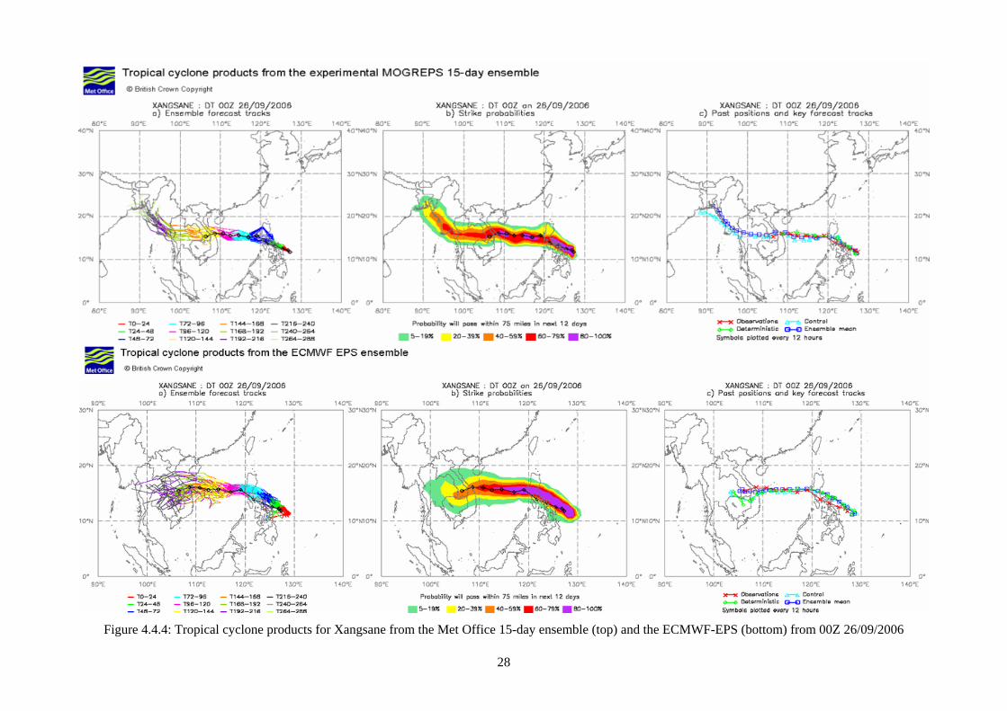
b) After the cyclone was named i.e. 00Z 26/09/2006 onwards Once a cyclone has been identified and named three products are produced: a) forecast tracks by each ensemble member; b) strike probability plot c) plot of deterministic track, control and ensemble mean. Figure 4.4.4 shows these products, with the observed track overlain, for DT 00Z 26/09/2006, the first run after the naming of Xangsane. The MOGREPS-15 ensemble performs very well, with the observed track falling within the spread throughout. The timing of the landfall in the Philippines is well predicted, and a cluster of tracks show the correct track across the country. The timing and track across the South China Sea is very good, with the ensemble mean closer to the observed track than the deterministic model. A very high probability is shown for the correct timing and location of landfall in Vietnam at T+120. By contrast, most of the members in the ECMWF EPS have the analysed position of the storm too far to the east, and track too far north over the Philippines, with the observed track outside of the ensemble spread. The timing of landfall is also slow by 24 hours. The track across the South China Sea is well within the spread of the ensemble, but again the forecast speed of the storm is too slow, with most members predicting landfall in Vietnam on 3rd October, 2 days later than observed. Figure 4.4.5 shows the same plots for the model runs 12 hours later, at 12Z 26/09/2006. The ECMWF EPS now performs better than MOGREPS-15, with the observed track within the spread throughout, and the problems with the speed of the storm from the previous data time overcome. The MOGREPS-15 ensemble follows the deterministic model too closely, predicting the storm to track over the northern part of Luzon. The observed, more southerly, track of the storm is outside of the ensemble spread, indicating that the model is under-spread and has not captured the uncertainty in this early part of the track. The timing and location of landfall in Vietnam, continues to be well predicted. The ensemble forecasts for DT 00Z 28/09/06, by which time Xangsane is crossing the Philippines, are shown in Figure 4.4.6. Although there is little spread in the tracks of the MOGREPS-15 ensemble, the track and speed of the storm across the South China Sea are well captured, showing good precision. The ECMWF EPS has a similar small level of spread around its deterministic model for the first 96 hours of the forecast, but the true landfall location in Vietnam is outside of the spread. Conclusion Xangsane was a particularly high-impact tropical cyclone as it passed so close to densely populated areas in the Philippines and Vietnam. Both ensembles show tropical cyclone genesis up to 4 days into the forecast in the correct region, with MOGREPS-15 showing greater predictive skill for the speed and track. Once Xangsane is named, the performance of the ensembles varies run to run. Both models follow their deterministic run too closely at times, with the true track outside of the spread. However, the timing and location of landfall in Vietnam is consistently better in MOGREPS-15, and the model could have provided valuable additional guidance to emergency planners. At times the MOGREPS-15
26
27
ensemble mean tracks closer to the observations than the deterministic model, which is encouraging, although further cases are needed in order to examine this in more detail. MOGREPS-15 clearly has a smaller spread than ECMWF, which in this case was better as the observed track generally stayed within that spread. However, the smaller spread of MOGREPS has been noted in other less predictable cases, such as Tropical Cyclone George in early March 2007. George made an abrupt left-hand turn to track south and cross the NW coast of Australia. This turn was missed by the deterministic model, and was not captured by the MOGREPS ensemble at several data times. The greater spread of the ECMWF ensemble did give some suggestion that a left turn was a possibility even though the actual track still fell outside the spread in most cases. More case studies are required to see whether the ECMWF EPS better captures the actual track in other less predictable cases.
Figure 4.4.4: Tropical cyclone products for Xangsane from the Met Office 15-day ensemble (top) and the ECMWF-EPS (bottom) from 00Z 26/09/2006
28
Figure 4.4.5: Tropical cyclone products for Xangsane from the Met Office 15-day ensemble (top) and the ECMWF-EPS (bottom) from 12Z 26/09/2006
29
30
Figure 4.4.6: Tropical cyclone products for Xangsane from the Met Office 15-day ensemble (top) and the ECMWF-EPS (bottom) from 00Z 28/09/2006
5. Objective Verification 5.1 Introduction Objective verification data has been calculated using the area-based verification (VER) system for the MOGREPS-15 ensemble since June 2006 and for the ECMWF ensemble since the beginning of 2007. The statistics calculated include the bias, root mean square error (RMS error), and spread using the ensemble mean or control, and probabilistic scores calculated using reliability table data. Verification has been performed both against observations and the analysis. Due to the constraint of transferring ECMWF verification data efficiently, we have focused upon three diagnostic fields: the pressure at mean sea-level (PMSL), the geopotential height at 500hPa (Z500), and the temperature at 850hPa (T850). 5.2 Continuous (single-field) verification The single-field graphs shown in this section are based on data gathered between 1 January 2007 and 15 November 2007. The mean values for biases, RMS errors and spreads at each forecast range are calculated from cases where both ECMWF and MOGREPS-15 statistics were available. PMSL Z500 T850
Figure 5.1: Verification against analysis: RMS errors for the control (solid) and ensemble mean
(dashed) in the northern hemisphere. ECMWF is plotted in blue, Met Office in red. Units are PMSL:Pa, Z500:metres, T850:ºC. Errors are as a result of calculating 90% confidence intervals using
a Monte-Carlo technique. Figure 5.1 shows the RMS error of the ensemble mean when verifying against analyses in the northern hemisphere (NH). The RMS error of the ensemble mean for the ECMWF ensemble is generally about 12 hours more skilful than the Met Office at lead times of 3 to 5 days (e.g. the RMS error of the Met Office forecast at 4½ days is approximately equal to the RMS error of the ECMWF forecast at 5 days). In the range 6 to 10 days, the ECMWF ensemble is more skilful by around 24 hours. The RMS error for the ensemble mean is consistently less than the RMS error for the control. This is expected as the ensemble should display greater skill than the control forecast alone. When verifying against observations, surface observations are used for PMSL, and sonde observations are used for both Z500 and T850. Plots of the mean RMS error of the ensemble mean against forecast range for verification against observations are similar to the curves shown in Figure 5.1, so Figure 5.2 shows the percentage difference between the RMS errors for MOGREPS-15 and ECMWF for four
31
areas. Differences are with respect to the mean RMS error of the MOGREPS-15 ensemble mean, so positive values represent a smaller MOGREPS-15 RMS error. PMSL Z500 T850
Figure 5.2: Verification against observations: Percentage difference in RMS error with respect to
MOGREPS-15. The four areas are the northern hemisphere (NH – in red), southern hemisphere (SH – in green), tropics (in blue) and North Atlantic-European area (NAE - in yellow).
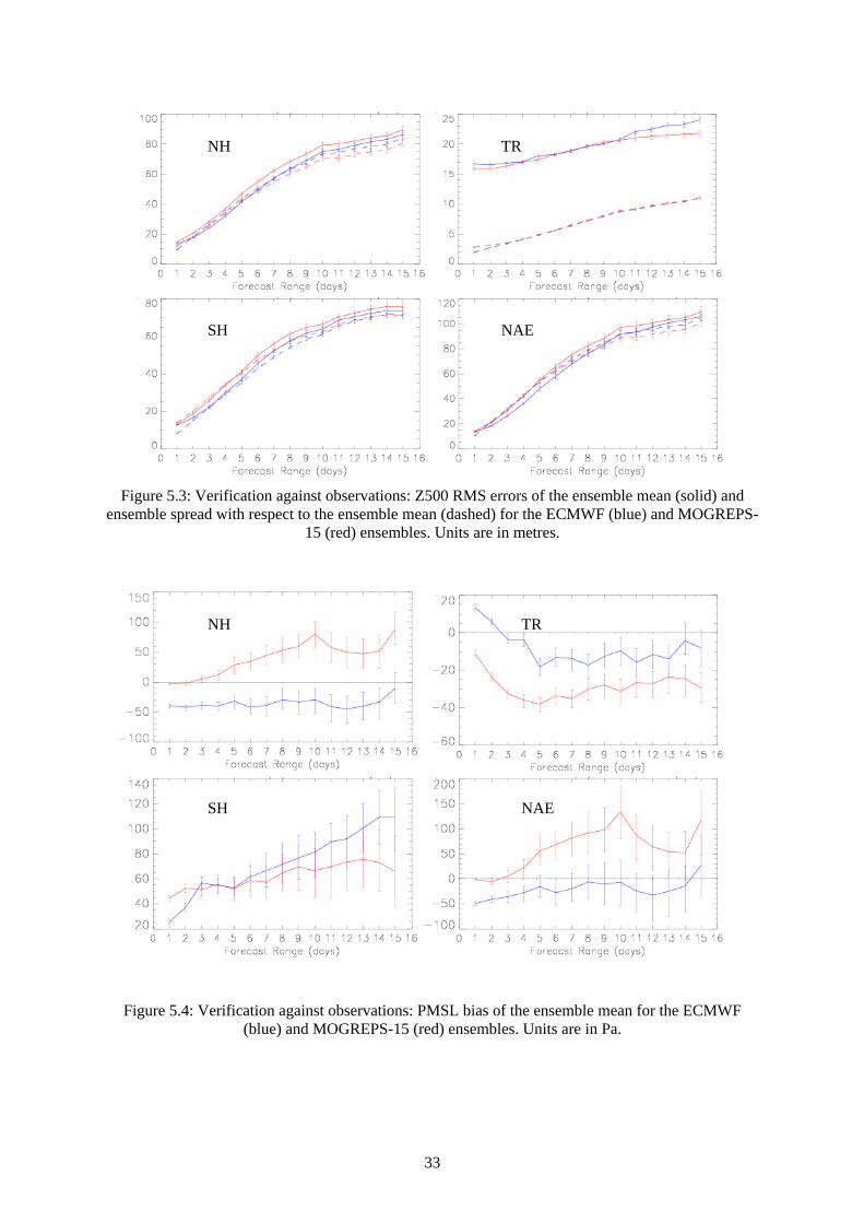
Firstly it is worth noting that similar trends are evident for all three fields. Secondly, it is clearly evident that for the MOGREPS-15 ensemble mean, the best performance relevant to ECMWF is in the tropics where the RMS error is either very close to, or lower than that of the ECMWF ensemble mean, in some cases up to 10% lower. The best performance in the tropics appears to be at lead times less than 3 days and greater than 10 days. For all other areas, the MOGREPS-15 ensemble mean performs worst against ECMWF at a lead time of approximately 3 days, and then steadily recovers towards longer lead-times. The perturbations for the ECMWF ensemble are based on singular vectors (sampling the space of errors that are likely to grow in the future) whilst the Met Office ensemble perturbations are based on the ETKF (sampling the space of errors that have grown in the past). Despite this difference, the spread of the ensembles are on the whole very similar. The ensemble spread is intended to reflect the uncertainty in the forecast; hence the spread of the ensemble around the ensemble mean should reflect the RMS error. The graphs in Figure 5.3 reveal that both ensembles are significantly under-spread in the tropics. In the SH, both ensembles are marginally under-spread. It is only in the NH that the ECMWF ensemble has sufficient spread, but the Met Office ensemble is marginally under-spread. The fact that the ensembles are under-spread to the degree seen in the tropics means that the verifying analysis is unlikely to be within the ensemble plume. Study of the bias of the ensemble mean with respect to observations reveals that both models perform well. In Figure 5.4, the bias for PMSL is displayed for the four different areas. In no case does the bias exceed 100Pa to any great degree. MOGREPS-15 performs at best against the ECMWF ensemble in the SH where the bias for both models is positive. The ECMWF bias is negative in the other three areas but remains very small. The MOGREPS-15 bias is of a larger magnitude, positive in the NH and negative in the tropics.
32
NH TR SH NAE
Figure 5.3: Verification against observations: Z500 RMS errors of the ensemble mean (solid) and ensemble spread with respect to the ensemble mean (dashed) for the ECMWF (blue) and MOGREPS-
15 (red) ensembles. Units are in metres. NH TR SH NAE
Figure 5.4: Verification against observations: PMSL bias of the ensemble mean for the ECMWF (blue) and MOGREPS-15 (red) ensembles. Units are in Pa.
33
For the fields Z500 (Figure 5.5) and T850 (not shown), MOGREPS-15 performs very well in both the tropics and southern hemisphere, where the bias is smaller than that of the ECMWF model. For Z500, the MOGREPS-15 bias in these two areas is generally less than 5 metres or less than 0.2ºC for T850. In the NH and NAE area, the situation is reversed and the ECMWF model performs better. The positive MOGREPS-15 bias increases with lead time to +15 metres for Z500. For T850 the bias is negative and does not exceed -0.3ºC. NH TR SH NAE Figure 5.5: Verification against observations: Z500 bias of the ensemble mean for the ECMWF (blue)
and MOGREPS-15 (red) ensembles. Units are in metres. 5.3 Categorical (probabilistic) verification As well as assessing the ensemble mean or control individually, the performance of the ensemble may be measured by constructing reliability tables. This data is calculated by binning the ensemble data according to a requested explicit threshold. Reliability tables have been derived over the period 3 March 2007 to 15 November 2007. In Figure 5.6, we present reliability diagrams for the threshold PMSL > 1020hPa in the NH. The trends seen in these graphs are representative of the performance of the MOGREPS-15 ensemble compared to the ECMWF ensemble in the NH and SH. In the top-most graphs it is evident that at T+24, MOGREPS-15 is more reliable, because the ECMWF ensemble is clearly under-forecasting the probability of the event occurring. As the lead time increases, the ECMWF ensemble becomes more reliable, but the MOGREPS-15 ensemble gradually begins to over-forecast the probability of 1020hPa being exceeded. The Brier Skill Score (BSS) assesses the relative skill of the probabilistic forecast over that of climatology. The dashed lines lying close to zero in Figure 5.7 represent the reliability of the ensembles and the closer to zero the more reliable the forecast at the lead time in question. The dotted lines in the same figure show the resolution of the forecast: the ability of the forecast to distinguish between different outcomes (hence climatology is represented by a horizontal line on a reliability diagram). In this case the higher the resolution the better. The BSS (solid line) is then a product of combining the reliability, resolution, and uncertainty in the forecast, and again higher is better, where a value of 1 is a perfect forecast.
34
T+24 T+24 T+120 T+120 T+240 T+240 Figure 5.6: Reliability diagrams versus observations in the NH for threshold PMSL > 1020. Plots for MOGREPS-15 are on the left in red; ECMWF on the right in blue. The ‘sharpness’ chart on each plot
displays the number of forecasts in each bin.
35
Figure 5.7: Brier Skill Score for PMSL > 1020hPa versus observations for the MOGREPS-15 ensemble (red) and ECMWF ensemble (blue).
Figure 5.7 shows the BSS for the threshold, PMSL > 1020hPa in the NH. The ECMWF has a better BSS at all lead times with the exception of T+24. The MOGREPS-15 is most competitive at lead times smaller than T+72 and greater than T+240. A similar trend can be seen when deriving the ‘area under ROC curve’ graph (Figure 5.8). The ROC (Relative Operating Characteristic) curve is the ability of the forecast to discriminate between events and non-events. A perfect forecast would be one that forecast all events, whilst registering no ‘false-alarms’, and the area under the ROC curve would be 1. A forecast having no skill would consequently be one where events and non-events are forecast in equal number, and the area under the ROC curve would be 0.5. The ECMWF ensemble performs better than MOGREPS-15, again with the exception of the forecast at T+24.
Figure 5.8: Area under ROC curve for PMSL > 1020hPa versus observations for the MOGREPS-15 ensemble (red) and ECMWF ensemble (blue).
36
Figure 5.9: BSS curves for PMSL < 990 (top) T850 > 283.15ºC (left) and Z500 > 564m (right) versus observations for the MOGREPS-15 ensemble (red) and ECMWF ensemble (blue). The graphs include
the reliability (dashed line), resolution (dotted line) and derived BSS score (solid line). Further BSS curves are presented for the NH in Figure 5.9. Study of all 3 fields suggests that the ECMWF ensemble generally outperforms the MOGREPS-15 ensemble with a gain in predictability of between 12 and 36 hours dependent upon the lead time. 5.4 Conclusions and further work A look at the single-field and probabilistic verification statistics has revealed that the ECMWF ensemble generally performs better than MOGREPS-15. However, it is encouraging that MOGREPS-15 is competitive despite the difference in development times of the two ensembles. In fact MOGREPS-15 has been shown that it can outperform the ECMWF ensemble at particular lead times and in particular areas, notably at T<72hrs and in the tropics. This fits with our hypothesis that MOGREPS-15 should benefit from the ‘tuning’ of the ensemble to the short-range, and benefit in the tropics where particular effort has been taken to improve performance in the deterministic model. In terms of the development of the verification system, it is intended that we should be able to calculate reliability statistics with respect to climatological percentiles rather than explicit thresholds. This will enable us to examine more closely the performance of MOGREPS-15 in the tropics where explicit thresholds, particular those for PMSL and Z500 are not very useful. We have also recently added 2m temperature to the ECMWF output data stream allowing us to compare performance using this important diagnostic.
37
6. Discussion and Conclusions This report has compared the medium-range ensemble forecasts from the Met Office (MOGREPS-15) with those from ECMWF (EPS/VAREPS). It was shown that the systematic model errors are comparable in the two systems. In some instances, the Met Office biases were smaller, in other examples, the ECMWF biases were smaller, though overall the ECMWF model generally had the edge. While systematic model errors are important, the key issue is: are the ensembles good at forecasting high-impact weather. Using a set of case studies, we have compared the guidance available from the two ensembles, using a range of diagnostic tools developed under the THORPEX project. It was found that there were some aspects where the guidance from MOGREPS-15 was better, and other cases where ECMWF gave a better indication of high-impact weather. This indicates scope for a multi-model ensemble to pick up the most skilful aspects of each of the component forecasts; future reports will evaluate the impact of multi-model ensemble techniques. To complement the case studies, we have also considered objective verification statistics. A range of different statistics show that the ECMWF ensemble generally performs better than MOGREPS-15. However, it is encouraging that MOGREPS-15 is generally competitive despite the difference in development times of the two ensemble forecast systems. Taken together, the results indicate that the performance is certainly comparable. There is every prospect of gaining from a multi-model medium-range ensemble by combining ensembles Met Office, ECMWF and other leading centres. The performance of MOGREPS is perfectly respectable compared to ECMWF, especially considering higher resolution of ECMWF. The results in this report were produced using either the original (HadGEMminus) or first updated (PS11/G39) set of physical parametrizations. More recently, a second upgrade (PS15/G44) has been implemented, which reduces some of the model biases. In conclusion, the prospects for a possible future multi-model medium-range ensemble forecast look very promising.
38
References. Bishop, C.H., B. J. Etherton, and S. J. Majumdar, 2001: ‘Adaptive sampling with the ensemble transform Kalman Filter. Part I: Theoretical aspects’ Mon. Weather Review, 129(3):420-436.
Bowler, N.E., A. Arribas, K. Mylne, and K. Robertson, 2007a: ‘Met Office Global and Regional Ensemble Prediction System (MOGREPS) Part I: System description’, NWP Technical Report 497, Met Office.
Bowler, N.E., A. Arribas, K. Mylne, and K. Robertson, 2007b: ‘Met Office Global and Regional Ensemble Prediction System (MOGREPS) Part II: Case Studies, Performance and Verification’, NWP Technical Report 498, Met Office.
Buizza, R. and T.N. Palmer, 1995: ‘The singular-vector structure of the atmospheric global circulation’, J. Atmos. Sci., 52, 1434-1456.
Buizza, R., M. Miller and T.N. Palmer, 1999: ‘Stochastic representation of model uncertainties in the ECMWF ensemble prediction system’, Quart. J. R. Meteorol. Soc., 125, 2887-2908.
Buizza, R., J.-R. Bidlot, N. Wedi, M. Fuentes, M. Hamrud, G. Holt and F. Vitart, 2007: ‘The new ECMWF VAREPS (Variable Resolution Ensemble Prediction System)’, Quart. J. Roy. Meteorol. Soc., submitted.
Hagedorn R., F.J. Doblas-Reyes, T.N. Palmer, 2005: ‘The rationale behind the success of multi-model ensembles in seasonal forecasting - I. Basic concept’, Tellus, A 57 (3): 219-233.
Harrison, M.S.J., Palmer,T.N., Richardson,D.S., Buizza,R., and Petroliagis, T., 1995: ‘Joint Ensembles from the UKMO and ECMWF Models’, ECMWF Seminar Proceedings on 'Predictability', 4-8 Sep 1995.
Jung T. and A. Tompkins, 2003: ‘Systematic Errors in the ECMWF Forecasting System’, Technical Memorandum 422, ECMWF.
Jung, T., 2003: ‘Systematic errors of the atmospheric circulation in the ECMWF forecasting system’, Quart. J. Roy. Meteorol. Soc., 131, 1045-1073.
Martin, G.M., M.A. Ringer, V.D. Pope, A. Jones, C. Dearden and T.J. Hinton, 2005: ‘The physical properties of the atmosphere in the new Hadley Centre Global Environmental Model (Had GEM1). Part 1: Model Description and global climatology’, J. Climate, 19, 1274-1301.
Milton, S.F., J. Heming D.Walters, and M. Willet, 2007: ‘A preliminary assessement of the performance of the Global Unified Model in THORPEX 15-day forecasts’, Forecasting Research Technical Report 495, Met Office.
Molteni, F., R. Buizza, T.N. Palmer and T. Petroliagis, 1996: ‘The ECMWF ensemble prediction system: methodology and validation’, Quart. J. Roy. Meteorol. Soc., 122, 73-119.
Palmer, T.N. et al, 2004: ‘Development of a European multimodel ensemble system for seasonal-to-interannual prediction (DEMETER)’, Bull. Amer. Meteorol. Soc., 85 (6), 853-872.
Rawlins F.R., S.P Ballard, K.J. Bovis, A.M. Clayton, D. Li, G.W. Inverarity, A.C. Lorenc and T.J. Payne, 2007: ‘The Met Office Global 4-Dimensional Variational Data Assimilation Scheme’, Quart. J. Roy. Meteorol. Soc., submitted.
Savage, N., S. Milton, D. Walters and J. Heming, 2007: An assessment of the imnpact of new physical parameterisations on the performance of the Global Unified Model in THORPEX 15-day forecasts’, Forecasting Research Technical Report 496, Met Office.
Savage, N., 2007: Impacts on THORPEX 15-day forecasts of model changes to address summer warm bias issues and other model changes, unpublished internal report, Met Office
Semple, A., 2007: Daily Weather Summaries, unpublished internal web pages, Met Office.