CD-ROM 6010B - 1 Revision 2 December 1996 METHOD 6010B INDUCTIVELY COUPLED PLASMA-ATOMIC EMISSION SPECTROMETRY 1.0 SCOPE AND APPLICATION 1.1 Inductively coupled plasma-atomic emission spectrometry (ICP-AES) determines trace elements, including metals, in solution. The method is applicable to all of the elements listed in Table 1. All matrices, excluding filtered groundwater samples but including ground water, aqueous samples, TCLP and EP extracts, industrial and organic wastes, soils, sludges, sediments, and other solid wastes, require digestion prior to analysis. Groundwater samples that have been prefiltered and acidified will not need acid digestion. Samples which are not digested must either use an internal standard or be matrix matched with the standards. Refer to Chapter Three for the appropriate digestion procedures. 1.2 Table 1 lists the elements for which this method is applicable. Detection limits, sensitivity, and the optimum and linear concentration ranges of the elements can vary with the wavelength, spectrometer, matrix and operating conditions. Table 1 lists the recommended analytical wavelengths and estimated instrumental detection limits for the elements in clean aqueous matrices. The instrument detection limit data may be used to estimate instrument and method performance for other sample matrices. Elements and matrices other than those listed in Table 1 may be analyzed by this method if performance at the concentration levels of interest (see Section 8.0) is demonstrated. 1.3 Users of the method should state the data quality objectives prior to analysis and must document and have on file the required initial demonstration performance data described in the following sections prior to using the method for analysis. 1.4 Use of this method is restricted to spectroscopists who are knowledgeable in the correction of spectral, chemical, and physical interferences described in this method. 2.0 SUMMARY OF METHOD 2.1 Prior to analysis, samples must be solubilized or digested using appropriate Sample Preparation Methods (e.g. Chapter Three). When analyzing groundwater samples for dissolved constituents, acid digestion is not necessary if the samples are filtered and acid preserved prior to analysis. 2.2 This method describes multielemental determinations by ICP-AES using sequential or simultaneous optical systems and axial or radial viewing of the plasma. The instrument measures characteristic emission spectra by optical spectrometry. Samples are nebulized and the resulting aerosol is transported to the plasma torch. Element-specific emission spectra are produced by a radio-frequency inductively coupled plasma. The spectra are dispersed by a grating spectrometer, and the intensities of the emission lines are monitored by photosensitive devices. Background correction is required for trace element determination. Background must be measured adjacent to analyte lines on samples during analysis. The position selected for the background-intensity measurement, on either or both sides of the analytical line, will be determined by the complexity of the spectrum adjacent to the analyte line. In one mode of analysis the position used should be as free as possible from spectral interference and should reflect the same change in background
1.1 Inductively coupled plasma-atomic emission spectrometry (ICP-AES) determinestrace elements, including metals, in solution. The method is applicable to all of the elements listedin Table 1. All matrices, excluding filtered groundwater samples but including ground water,aqueous samples, TCLP and EP extracts, industrial and organic wastes, soils, sludges, sediments,and other solid wastes, require digestion prior to analysis. Groundwater samples that have beenprefiltered and acidified will not need acid digestion. Samples which are not digested must eitheruse an internal standard or be matrix matched with the standards. Refer to Chapter Three for theappropriate digestion procedures.
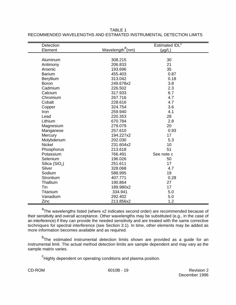
1.2 Table 1 lists the elements for which this method is applicable. Detection limits,sensitivity, and the optimum and linear concentration ranges of the elements can vary with thewavelength, spectrometer, matrix and operating conditions. Table 1 lists the recommendedanalytical wavelengths and estimated instrumental detection limits for the elements in clean aqueousmatrices. The instrument detection limit data may be used to estimate instrument and methodperformance for other sample matrices. Elements and matrices other than those listed in Table 1may be analyzed by this method if performance at the concentration levels of interest (see Section8.0) is demonstrated.
1.3 Users of the method should state the data quality objectives prior to analysis and mustdocument and have on file the required initial demonstration performance data described in thefollowing sections prior to using the method for analysis.
1.4 Use of this method is restricted to spectroscopists who are knowledgeable in thecorrection of spectral, chemical, and physical interferences described in this method.
2.0 SUMMARY OF METHOD
2.1 Prior to analysis, samples must be solubilized or digested using appropriate SamplePreparation Methods (e.g. Chapter Three). When analyzing groundwater samples for dissolvedconstituents, acid digestion is not necessary if the samples are filtered and acid preserved prior toanalysis.
2.2 This method describes multielemental determinations by ICP-AES using sequential orsimultaneous optical systems and axial or radial viewing of the plasma. The instrument measurescharacteristic emission spectra by optical spectrometry. Samples are nebulized and the resultingaerosol is transported to the plasma torch. Element-specific emission spectra are produced by aradio-frequency inductively coupled plasma. The spectra are dispersed by a grating spectrometer,and the intensities of the emission lines are monitored by photosensitive devices. Backgroundcorrection is required for trace element determination. Background must be measured adjacent toanalyte lines on samples during analysis. The position selected for the background-intensitymeasurement, on either or both sides of the analytical line, will be determined by the complexity ofthe spectrum adjacent to the analyte line. In one mode of analysis the position used should be asfree as possible from spectral interference and should reflect the same change in background
CD-ROM 6010B - 2 Revision 2December 1996
intensity as occurs at the analyte wavelength measured. Background correction is not required incases of line broadening where a background correction measurement would actually degrade theanalytical result. The possibility of additional interferences named in Section 3.0 should also berecognized and appropriate corrections made; tests for their presence are described in Section 8.5.Alternatively, users may choose multivariate calibration methods. In this case, point selections forbackground correction are superfluous since whole spectral regions are processed.
3.0 INTERFERENCES
3.1 Spectral interferences are caused by background emission from continuous orrecombination phenomena, stray light from the line emission of high concentration elements, overlapof a spectral line from another element, or unresolved overlap of molecular band spectra.
3.1.1 Background emission and stray light can usually be compensated for bysubtracting the background emission determined by measurements adjacent to the analytewavelength peak. Spectral scans of samples or single element solutions in the analyteregions may indicate when alternate wavelengths are desirable because of severe spectralinterference. These scans will also show whether the most appropriate estimate of thebackground emission is provided by an interpolation from measurements on both sides ofthe wavelength peak or by measured emission on only one side. The locations selected forthe measurement of background intensity will be determined by the complexity of thespectrum adjacent to the wavelength peak. The locations used for routine measurementmust be free of off-line spectral interference (interelement or molecular) or adequatelycorrected to reflect the same change in background intensity as occurs at the wavelengthpeak. For multivariate methods using whole spectral regions, background scans should beincluded in the correction algorithm. Off-line spectral interferences are handled by includingspectra on interfering species in the algorithm.
3.1.2 To determine the appropriate location for off-line background correction, theuser must scan the area on either side adjacent to the wavelength and record the apparentemission intensity from all other method analytes. This spectral information must bedocumented and kept on file. The location selected for background correction must be eitherfree of off-line interelement spectral interference or a computer routine must be used forautomatic correction on all determinations. If a wavelength other than the recommendedwavelength is used, the analyst must determine and document both the overlapping andnearby spectral interference effects from all method analytes and common elements andprovide for their automatic correction on all analyses. Tests to determine spectralinterference must be done using analyte concentrations that will adequately describe theinterference. Normally, 100 mg/L single element solutions are sufficient; however, foranalytes such as iron that may be found at high concentration, a more appropriate test wouldbe to use a concentration near the upper analytical range limit.
3.1.3 Spectral overlaps may be avoided by using an alternate wavelength or can becompensated by equations that correct for interelement contributions. Instruments that useequations for interelement correction require the interfering elements be analyzed at thesame time as the element of interest. When operative and uncorrected, interferences willproduce false positive determinations and be reported as analyte concentrations. Moreextensive information on interferant effects at various wavelengths and resolutions isavailable in reference wavelength tables and books. Users may apply interelement
CD-ROM 6010B - 3 Revision 2December 1996
correction equations determined on their instruments with tested concentration ranges tocompensate (off line or on line) for the effects of interfering elements. Some potentialspectral interferences observed for the recommended wavelengths are given in Table 2. Formultivariate methods using whole spectral regions, spectral interferences are handled byincluding spectra of the interfering elements in the algorithm. The interferences listed areonly those that occur between method analytes. Only interferences of a direct overlap natureare listed. These overlaps were observed with a single instrument having a workingresolution of 0.035 nm.
3.1.4 When using interelement correction equations, the interference may beexpressed as analyte concentration equivalents (i.e. false analyte concentrations) arisingfrom 100 mg/L of the interference element. For example, assume that As is to bedetermined (at 193.696 nm) in a sample containing approximately 10 mg/L of Al. Accordingto Table 2, 100 mg/L of Al would yield a false signal for As equivalent to approximately 1.3mg/L. Therefore, the presence of 10 mg/L of Al would result in a false signal for Asequivalent to approximately 0.13 mg/L. The user is cautioned that other instruments mayexhibit somewhat different levels of interference than those shown in Table 2. Theinterference effects must be evaluated for each individual instrument since the intensities willvary.
3.1.5 Interelement corrections will vary for the same emission line amonginstruments because of differences in resolution, as determined by the grating, the entranceand exit slit widths, and by the order of dispersion. Interelement corrections will also varydepending upon the choice of background correction points. Selecting a backgroundcorrection point where an interfering emission line may appear should be avoided whenpractical. Interelement corrections that constitute a major portion of an emission signal maynot yield accurate data. Users should not forget that some samples may contain uncommonelements that could contribute spectral interferences.
3.1.6 The interference effects must be evaluated for each individual instrumentwhether configured as a sequential or simultaneous instrument. For each instrument,intensities will vary not only with optical resolution but also with operating conditions (suchas power, viewing height and argon flow rate). When using the recommended wavelengths,the analyst is required to determine and document for each wavelength the effect fromreferenced interferences (Table 2) as well as any other suspected interferences that may bespecific to the instrument or matrix. The analyst is encouraged to utilize a computer routinefor automatic correction on all analyses.
3.1.7 Users of sequential instruments must verify the absence of spectralinterference by scanning over a range of 0.5 nm centered on the wavelength of interest forseveral samples. The range for lead, for example, would be from 220.6 to 220.1 nm. Thisprocedure must be repeated whenever a new matrix is to be analyzed and when a newcalibration curve using different instrumental conditions is to be prepared. Samples thatshow an elevated background emission across the range may be background corrected byapplying a correction factor equal to the emission adjacent to the line or at two points oneither side of the line and interpolating between them. An alternate wavelength that doesnot exhibit a background shift or spectral overlap may also be used.
CD-ROM 6010B - 4 Revision 2December 1996
3.1.8 If the correction routine is operating properly, the determined apparentanalyte(s) concentration from analysis of each interference solution should fall within aspecific concentration range around the calibration blank. The concentration range iscalculated by multiplying the concentration of the interfering element by the value of thecorrection factor being tested and divided by 10. If after the subtraction of the calibrationblank the apparent analyte concentration falls outside of this range in either a positive ornegative direction, a change in the correction factor of more than 10% should be suspected.The cause of the change should be determined and corrected and the correction factorupdated. The interference check solutions should be analyzed more than once to confirma change has occurred. Adequate rinse time between solutions and before analysis of thecalibration blank will assist in the confirmation.
3.1.9 When interelement corrections are applied, their accuracy should be verified,daily, by analyzing spectral interference check solutions. If the correction factors ormultivariate correction matrices tested on a daily basis are found to be within the 20% criteriafor 5 consecutive days, the required verification frequency of those factors in compliance maybe extended to a weekly basis. Also, if the nature of the samples analyzed is such they donot contain concentrations of the interfering elements at ± one reporting limit from zero, dailyverification is not required. All interelement spectral correction factors or multivariatecorrection matrices must be verified and updated every six months or when aninstrumentation change, such as in the torch, nebulizer, injector, or plasma conditionsoccurs. Standard solution should be inspected to ensure that there is no contamination thatmay be perceived as a spectral interference.
3.1.10 When interelement corrections are not used, verification of absence ofinterferences is required.
3.1.10.1 One method is to use a computer software routine for comparingthe determinative data to limits files for notifying the analyst when an interferingelement is detected in the sample at a concentration that will produce either anapparent false positive concentration, (i.e., greater than) the analyte instrumentdetection limit, or false negative analyte concentration, (i.e., less than the lowercontrol limit of the calibration blank defined for a 99% confidence interval).
3.1.10.2 Another method is to analyze an Interference Check Solution(s)which contains similar concentrations of the major components of the samples (>10mg/L) on a continuing basis to verify the absence of effects at the wavelengthsselected. These data must be kept on file with the sample analysis data. If thecheck solution confirms an operative interference that is > 20% of the analyteconcentration, the analyte must be determined using (1) analytical and backgroundcorrection wavelengths (or spectral regions) free of the interference, (2) by analternative wavelength, or (3) by another documented test procedure.
3.2 Physical interferences are effects associated with the sample nebulization andtransport processes. Changes in viscosity and surface tension can cause significant inaccuracies,especially in samples containing high dissolved solids or high acid concentrations. If physicalinterferences are present, they must be reduced by diluting the sample or by using a peristalticpump, by using an internal standard or by using a high solids nebulizer. Another problem that canoccur with high dissolved solids is salt buildup at the tip of the nebulizer, affecting aerosol flow rate
CD-ROM 6010B - 5 Revision 2December 1996
and causing instrumental drift. The problem can be controlled by wetting the argon prior tonebulization, using a tip washer, using a high solids nebulizer or diluting the sample. Also, it hasbeen reported that better control of the argon flow rate, especially to the nebulizer, improvesinstrument performance: this may be accomplished with the use of mass flow controllers. The testdescribed in Section 8.5.1 will help determine if a physical interference is present.
3.3 Chemical interferences include molecular compound formation, ionization effects, andsolute vaporization effects. Normally, these effects are not significant with the ICP technique, butif observed, can be minimized by careful selection of operating conditions (incident power,observation position, and so forth), by buffering of the sample, by matrix matching, and by standardaddition procedures. Chemical interferences are highly dependent on matrix type and the specificanalyte element.
3.4 Memory interferences result when analytes in a previous sample contribute to thesignals measured in a new sample. Memory effects can result from sample deposition on the uptaketubing to the nebulizer and from the build up of sample material in the plasma torch and spraychamber. The site where these effects occur is dependent on the element and can be minimizedby flushing the system with a rinse blank between samples. The possibility of memory interferencesshould be recognized within an analytical run and suitable rinse times should be used to reducethem. The rinse times necessary for a particular element must be estimated prior to analysis. Thismay be achieved by aspirating a standard containing elements at a concentration ten times the usualamount or at the top of the linear dynamic range. The aspiration time for this sample should be thesame as a normal sample analysis period, followed by analysis of the rinse blank at designatedintervals. The length of time required to reduce analyte signals to within a factor of two of themethod detection limit should be noted. Until the required rinse time is established, this methodsuggests a rinse period of at least 60 seconds between samples and standards. If a memoryinterference is suspected, the sample must be reanalyzed after a rinse period of sufficient length.Alternate rinse times may be established by the analyst based upon their DQOs.
3.5 Users are advised that high salt concentrations can cause analyte signalsuppressions and confuse interference tests. If the instrument does not display negative values,fortify the interference check solution with the elements of interest at 0.5 to 1 mg/L and measure theadded standard concentration accordingly. Concentrations should be within 20% of the true spikedconcentration or dilution of the samples will be necessary. In the absence of measurable analyte,overcorrection could go undetected if a negative value is reported as zero.
3.6 The dashes in Table 2 indicate that no measurable interferences were observed evenat higher interferant concentrations. Generally, interferences were discernible if they producedpeaks, or background shifts, corresponding to 2 to 5% of the peaks generated by the analyteconcentrations.
4.1.1 Computer-controlled emission spectrometer with background correction.
4.1.2 Radio-frequency generator compliant with FCC regulations.
CD-ROM 6010B - 6 Revision 2December 1996
4.1.3 Optional mass flow controller for argon nebulizer gas supply.
4.1.4 Optional peristaltic pump.
4.1.5 Optional Autosampler.
4.1.6 Argon gas supply - high purity.
4.2 Volumetric flasks of suitable precision and accuracy.
4.3 Volumetric pipets of suitable precision and accuracy.
5.0 REAGENTS 5.1 Reagent or trace metals grade chemicals shall be used in all tests. Unless otherwiseindicated, it is intended that all reagents shall conform to the specifications of the Committee onAnalytical Reagents of the American Chemical Society, where such specifications are available.Other grades may be used, provided it is first ascertained that the reagent is of sufficiently high purityto permit its use without lessening the accuracy of the determination. If the purity of a reagent is inquestion analyze for contamination. If the concentration of the contamination is less than the MDLthen the reagent is acceptable.
5.1.1 Hydrochloric acid (conc), HCl.
5.1.2 Hydrochloric acid (1:1), HCl. Add 500 mL concentrated HCl to 400 mL waterand dilute to 1 liter in an appropriately sized beaker.
5.1.3 Nitric acid (conc), HNO .3
5.1.4 Nitric acid (1:1), HNO . Add 500 mL concentrated HNO to 400 mL water and3 3
dilute to 1 liter in an appropriately sized beaker.
5.2 Reagent Water. All references to water in the method refer to reagent water unlessotherwise specified. Reagent water will be interference free. Refer to Chapter One for a definitionof reagent water.
5.3 Standard stock solutions may be purchased or prepared from ultra- high purity gradechemicals or metals (99.99% pure or greater). All salts must be dried for 1 hour at 105EC, unlessotherwise specified.
Note: This section does not apply when analyzing samples that have been prepared byMethod 3040.
CAUTION: Many metal salts are extremely toxic if inhaled or swallowed. Wash handsthoroughly after handling.
Typical stock solution preparation procedures follow. Concentrations are calculated based upon theweight of pure metal added, or with the use of the element fraction and the weight of the metal saltadded.
CD-ROM 6010B - 7 Revision 2December 1996
For metals: weight (mg) Concentration (ppm) = ))))))))))) volume (L)
For metal salts: weight (mg) x mole fraction Concentration (ppm) = ))))))))))))))))))))))))))) volume (L)
5.3.1 Aluminum solution, stock, 1 mL = 1000 µg Al: Dissolve 1.000 g of aluminummetal, weighed accurately to at least four significant figures, in an acid mixture of 4.0 mL of(1:1) HCl and 1.0 mL of concentrated HN0 in a beaker. Warm beaker slowly to effect3
solution. When dissolution is complete, transfer solution quantitatively to a 1-liter flask, addan additional 10.0 mL of (1:1) HCl and dilute to volume with reagent water.
NOTE: Weight of analyte is expressed to four significant figures for consistency with theweights below because rounding to two decimal places can contribute up to 4 % error forsome of the compounds.
5.3.2 Antimony solution, stock, 1 mL = 1000 µg Sb: Dissolve 2.6673 gK(SbO)C H O (element fraction Sb = 0.3749), weighed accurately to at least four significant4 4 6
figures, in water, add 10 mL (1:1) HCl, and dilute to volume in a 1,000 mL volumetric flaskwith water.
5.3.3 Arsenic solution, stock, 1 mL = 1000 µg As: Dissolve 1.3203 g of As O2 3
(element fraction As = 0.7574), weighed accurately to at least four significant figures, in 100mL of water containing 0.4 g NaOH. Acidify the solution with 2 mL concentrated HNO and3
dilute to volume in a 1,000 mL volumetric flask with water.
5.3.4 Barium solution, stock, 1 mL = 1000 µg Ba: Dissolve 1.5163 g BaCl (element2
fraction Ba = 0.6595), dried at 250EC for 2 hours, weighed accurately to at least foursignificant figures, in 10 mL water with 1 mL (1:1) HCl. Add 10.0 mL (1:1) HCl and dilute tovolume in a 1,000 mL volumetric flask with water.
5.3.5 Beryllium solution, stock, 1 mL = 1000 µg Be: Do not dry. Dissolve 19.6463g BeSO 4H O (element fraction Be = 0.0509), weighed accurately to at least four significant4 2
.
figures, in water, add 10.0 mL concentrated HNO , and dilute to volume in a 1,000 mL3
volumetric flask with water.
5.3.6 Boron solution, stock, 1 mL = 1000 µg B: Do not dry. Dissolve 5.716 ganhydrous H BO (B fraction = 0.1749), weighed accurately to at least four significant figures,3 3
in reagent water and dilute in a 1-L volumetric flask with reagent water. Transfer immediatelyafter mixing in a clean polytetrafluoroethylene (PTFE) bottle to minimize any leaching ofboron from the glass volumetric container. Use of a non-glass volumetric flask isrecommended to avoid boron contamination from glassware.
5.3.7 Cadmium solution, stock, 1 mL = 1000 µg Cd: Dissolve 1.1423 g CdO(element fraction Cd = 0.8754), weighed accurately to at least four significant figures, in a
CD-ROM 6010B - 8 Revision 2December 1996
minimum amount of (1:1) HNO . Heat to increase rate of dissolution. Add 10.0 mL3
concentrated HNO and dilute to volume in a 1,000 mL volumetric flask with water.3
5.3.8 Calcium solution, stock, 1 mL = 1000 µg Ca: Suspend 2.4969 g CaCO3
(element Ca fraction = 0.4005), dried at 180EC for 1 hour before weighing, weighedaccurately to at least four significant figures, in water and dissolve cautiously with a minimumamount of (1:1) HNO . Add 10.0 mL concentrated HNO and dilute to volume in a 1,000 mL3 3
volumetric flask with water.
5.3.9 Chromium solution, stock, 1 mL = 1000 µg Cr: Dissolve 1.9231 g CrO3
(element fraction Cr = 0.5200), weighed accurately to at least four significant figures, inwater. When solution is complete, acidify with 10 mL concentrated HNO and dilute to3
volume in a 1,000 mL volumetric flask with water.
5.3.10 Cobalt solution, stock, 1 mL = 1000 µg Co: Dissolve 1.00 g of cobalt metal,weighed accurately to at least four significant figures, in a minimum amount of (1:1) HNO .3
Add 10.0 mL (1:1) HCl and dilute to volume in a 1,000 mL volumetric flask with water.
5.3.11 Copper solution, stock, 1 mL = 1000 µg Cu: Dissolve 1.2564 g CuO (elementfraction Cu = 0.7989), weighed accurately to at least four significant figures), in a minimumamount of (1:1) HNO . Add 10.0 mL concentrated HNO and dilute to volume in a 1,000 mL3 3
volumetric flask with water.
5.3.12 Iron solution, stock, 1 mL = 1000 µg Fe: Dissolve 1.4298 g Fe O (element2 3
fraction Fe = 0.6994), weighed accurately to at least four significant figures, in a warmmixture of 20 mL (1:1) HCl and 2 mL of concentrated HNO . Cool, add an additional 5.0 mL3
of concentrated HNO , and dilute to volume in a 1,000 mL volumetric flask with water.3
5.3.13 Lead solution, stock, 1 mL = 1000 µg Pb: Dissolve 1.5985 g Pb(NO )3 2
(element fraction Pb = 0.6256), weighed accurately to at least four significant figures, in aminimum amount of (1:1) HNO . Add 10 mL (1:1) HNO and dilute to volume in a 1,000 mL3 3
volumetric flask with water.
5.3.14 Lithium solution, stock, 1 mL = 1000 µg Li: Dissolve 5.3248 g lithiumcarbonate (element fraction Li = 0.1878), weighed accurately to at least four significantfigures, in a minimum amount of (1:1) HCl and dilute to volume in a 1,000 mL volumetricflask with water.
5.3.15 Magnesium solution, stock, 1 mL = 1000 µg Mg: Dissolve 1.6584 g MgO(element fraction Mg = 0.6030), weighed accurately to at least four significant figures, in aminimum amount of (1:1) HNO . Add 10.0 mL (1:1) concentrated HNO and dilute to volume3 3
in a 1,000 mL volumetric flask with water.
5.3.16 Manganese solution, stock, 1 mL = 1000 µg Mn: Dissolve 1.00 g ofmanganese metal, weighed accurately to at least four significant figures, in acid mixture (10mL concentrated HCl and 1 mL concentrated HNO ) and dilute to volume in a 1,000 mL3
volumetric flask with water.
CD-ROM 6010B - 9 Revision 2December 1996
5.3.17 Mercury solution, stock, 1 mL = 1000 µg Hg: Do not dry, highly toxic element.Dissolve 1.354 g HgCl (Hg fraction = 0.7388) in reagent water. Add 50.0 mL concentrated2
HNO and dilute to volume in 1-L volumetric flask with reagent water.3
5.3.18 Molybdenum solution, stock, 1 mL = 1000 µg Mo: Dissolve 1.7325 g(NH ) Mo O .4H O (element fraction Mo = 0.5772), weighed accurately to at least four4 6 7 24 2
significant figures, in water and dilute to volume in a 1,000 mL volumetric flask with water.
5.3.19 Nickel solution, stock, 1 mL = 1000 µg Ni: Dissolve 1.00 g of nickel metal,weighed accurately to at least four significant figures, in 10.0 mL hot concentrated HNO ,3
cool, and dilute to volume in a 1,000 mL volumetric flask with water.
5.3.20 Phosphate solution, stock, 1 mL = 1000 µg P: Dissolve 4.3937 g anhydrousKH PO (element fraction P = 0.2276), weighed accurately to at least four significant figures,2 4
in water. Dilute to volume in a 1,000 mL volumetric flask with water.
5.3.21 Potassium solution, stock, 1 mL = 1000 µg K: Dissolve 1.9069 g KCl (elementfraction K = 0.5244) dried at 110EC, weighed accurately to at least four significant figures,in water, and dilute to volume in a 1,000 mL volumetric flask with water.
5.3.22 Selenium solution, stock, 1 mL = 1000 µg Se: Do not dry. Dissolve 1.6332g H SeO (element fraction Se = 0.6123), weighed accurately to at least four significant2 3
figures, in water and dilute to volume in a 1,000 mL volumetric flask with water.
5.3.23 Silica solution, stock, 1 mL = 1000 µg SiO : Do not dry. Dissolve 2.964 g2
NH SiF , weighed accurately to at least four significant figures, in 200 mL (1:20) HCl with4 6
heating at 85EC to effect dissolution. Let solution cool and dilute to volume in a 1-Lvolumetric flask with reagent water.
5.3.24 Silver solution, stock, 1 mL = 1000 µg Ag: Dissolve 1.5748 g AgNO (element3
fraction Ag = 0.6350), weighed accurately to at least four significant figures, in water and 10mL concentrated HNO . Dilute to volume in a 1,000 mL volumetric flask with water.3
5.3.25 Sodium solution, stock, 1 mL = 1000 µg Na: Dissolve 2.5419 g NaCl (elementfraction Na = 0.3934), weighed accurately to at least four significant figures, in water. Add10.0 mL concentrated HNO and dilute to volume in a 1,000 mL volumetric flask with water.3
5.3.26 Strontium solution, stock, 1 mL = 1000 µg Sr: Dissolve 2.4154 g of strontiumnitrate (Sr(NO ) ) (element fraction Sr = 0.4140), weighed accurately to at least four3 2
significant figures, in a 1-liter flask containing 10 mL of concentrated HCl and 700 mL ofwater. Dilute to volume in a 1,000 mL volumetric flask with water.
5.3.27 Thallium solution, stock, 1 mL = 1000 µg Tl: Dissolve 1.3034 g TlNO3
(element fraction Tl = 0.7672), weighed accurately to at least four significant figures, in water.Add 10.0 mL concentrated HNO and dilute to volume in a 1,000 mL volumetric flask with3
water.
CD-ROM 6010B - 10 Revision 2December 1996
5.3.28 Tin solution, stock, 1 mL = 1000 µg Sn: Dissolve 1.000 g Sn shot, weighedaccurately to at least 4 significant figures, in 200 mL (1:1) HCl with heating to effectdissolution. Let solution cool and dilute with (1:1) HCl in a 1-L volumetric flask.
5.3.29 Vanadium solution, stock, 1 mL = 1000 µg V: Dissolve 2.2957 g NH VO4 3
(element fraction V = 0.4356), weighed accurately to at least four significant figures, in aminimum amount of concentrated HNO . Heat to increase rate of dissolution. Add 10.0 mL3
concentrated HNO and dilute to volume in a 1,000 mL volumetric flask with water.3
5.3.30 Zinc solution, stock, 1 mL = 1000 µg Zn: Dissolve 1.2447 g ZnO (elementfraction Zn = 0.8034), weighed accurately to at least four significant figures, in a minimumamount of dilute HNO . Add 10.0 mL concentrated HNO and dilute to volume in a 1,000 mL3 3
volumetric flask with water.
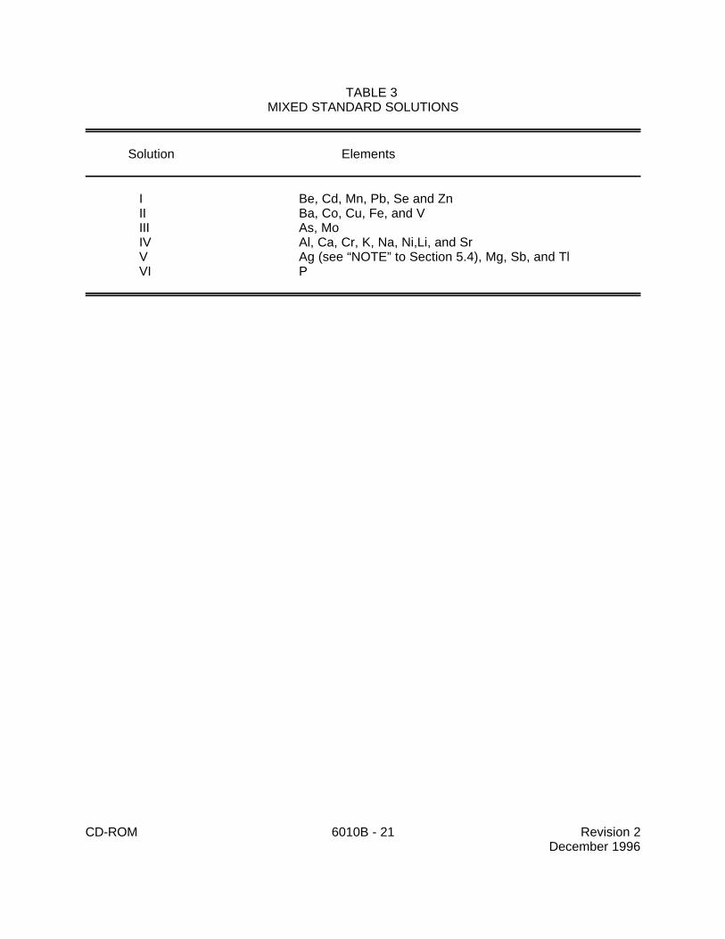
5.4 Mixed calibration standard solutions - Prepare mixed calibration standard solutions bycombining appropriate volumes of the stock solutions in volumetric flasks (see Table 3). Add theappropriate types and volumes of acids so that the standards are matrix matched with the sampledigestates. Prior to preparing the mixed standards, each stock solution should be analyzedseparately to determine possible spectral interference or the presence of impurities. Care shouldbe taken when preparing the mixed standards to ensure that the elements are compatible and stabletogether. Transfer the mixed standard solutions to FEP fluorocarbon or previously unusedpolyethylene or polypropylene bottles for storage. Fresh mixed standards should be prepared, asneeded, with the realization that concentration can change on aging. Some typical calibrationstandard combinations are listed in Table 3.
NOTE: If the addition of silver to the recommended acid combination results in an initialprecipitation, add 15 mL of water and warm the flask until the solution clears. Cool and diluteto 100 mL with water. For this acid combination, the silver concentration should be limitedto 2 mg/L. Silver under these conditions is stable in a tap-water matrix for 30 days. Higherconcentrations of silver require additional HCl.
5.5 Two types of blanks are required for the analysis for samples prepared by any methodother than 3040. The calibration blank is used in establishing the analytical curve, and the methodblank is used to identify possible contamination resulting from varying amounts of the acids used inthe sample processing.
5.5.1 The calibration blank is prepared by acidifying reagent water to the sameconcentrations of the acids found in the standards and samples. Prepare a sufficientquantity to flush the system between standards and samples. The calibration blank will alsobe used for all initial and continuing calibration blank determinations (see Sections 7.3 and7.4).
5.5.2 The method blank must contain all of the reagents in the same volumes asused in the processing of the samples. The method blank must be carried through thecomplete procedure and contain the same acid concentration in the final solution as thesample solution used for analysis.
CD-ROM 6010B - 11 Revision 2December 1996
5.6 The Initial Calibration Verification (ICV) is prepared by the analyst by combiningcompatible elements from a standard source different than that of the calibration standard and atconcentrations within the linear working range of the instrument (see Section 8.6.1 for use).
5.7 The Continuing Calibration Verification (CCV)) should be prepared in the same acidmatrix using the same standards used for calibration at a concentration near the mid-point of thecalibration curve (see Section 8.6.1 for use).
5.8 The interference check solution is prepared to contain known concentrations ofinterfering elements that will provide an adequate test of the correction factors. Spike the samplewith the elements of interest, particularly those with known interferences at 0.5 to 1 mg/L. In theabsence of measurable analyte, overcorrection could go undetected because a negative value couldbe reported as zero. If the particular instrument will display overcorrection as a negative number,this spiking procedure will not be necessary.
6.0 SAMPLE COLLECTION, PRESERVATION, AND HANDLING
6.1 See the introductory material in Chapter Three, Inorganic Analytes, Sections 3.1 through3.3.
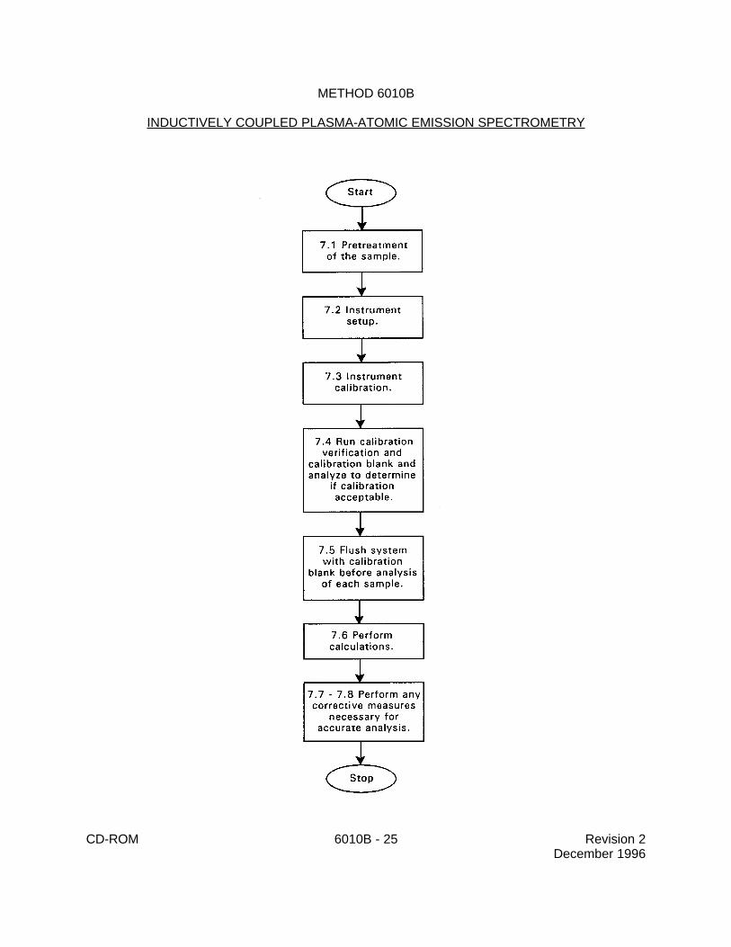
7.0 PROCEDURE
7.1 Preliminary treatment of most matrices is necessary because of the complexity andvariability of sample matrices. Groundwater samples which have been prefiltered and acidified willnot need acid digestion. Samples which are not digested must either use an internal standard orbe matrix matched with the standards. Solubilization and digestion procedures are presented inSample Preparation Methods (Chapter Three, Inorganic Analytes).
7.2 Set up the instrument with proper operating parameters established as detailed below.The instrument must be allowed to become thermally stable before beginning (usually requiring atleast 30 minutes of operation prior to calibration). Operating conditions - The analyst should followthe instructions provided by the instrument manufacturer.
7.2.1 Before using this procedure to analyze samples, there must be data availabledocumenting initial demonstration of performance. The required data document the selectioncriteria of background correction points; analytical dynamic ranges, the applicable equations,and the upper limits of those ranges; the method and instrument detection limits; and thedetermination and verification of interelement correction equations or other routines forcorrecting spectral interferences. This data must be generated using the same instrument,operating conditions and calibration routine to be used for sample analysis. Thesedocumented data must be kept on file and be available for review by the data user or auditor.
7.2.2 Specific wavelengths are listed in Table 1. Other wavelengths may besubstituted if they can provide the needed sensitivity and are corrected for spectralinterference. Because of differences among various makes and models of spectrometers,specific instrument operating conditions cannot be provided. The instrument and operatingconditions utilized for determination must be capable of providing data of acceptable qualityto the program and data user. The analyst should follow the instructions provided by theinstrument manufacturer unless other conditions provide similar or better performance for
CD-ROM 6010B - 12 Revision 2December 1996
a task. Operating conditions for aqueous solutions usually vary from 1100 to 1200 wattsforward power, 14 to 18 mm viewing height, 15 to 19 liters/min argon coolant flow, 0.6 to 1.5L/min argon nebulizer flow, 1 to 1.8 mL/min sample pumping rate with a 1 minute preflushtime and measurement time near 1 second per wavelength peak for sequential instrumentsand 10 seconds per sample for simultaneous instruments. For an axial plasma, theconditions will usually vary from 1100-1500 watts forward power, 15-19 liters/min argoncoolant flow, 0.6-1.5 L/min argon nebulizer flow, 1-1.8 mL/min sample pumping rate with a1 minute preflush time and measurement time near 1 second per wavelength peak forsequential instruments and 10 seconds per sample for simultaneous instruments.Reproduction of the Cu/Mn intensity ratio at 324.754 nm and 257.610 nm respectively, byadjusting the argon aerosol flow has been recommended as a way to achieve repeatableinterference correction factors.
7.2.3 The plasma operating conditions need to be optimized prior to use of theinstrument. This routine is not required on a daily basis, but only when first setting up a newinstrument or following a change in operating conditions. The following procedure isrecommended or follow manufacturer’s recommendations. The purpose of plasmaoptimization is to provide a maximum signal to background ratio for some of the leastsensitive elements in the analytical array. The use of a mass flow controller to regulate thenebulizer gas flow or source optimization software greatly facilitates the procedure.
7.2.3.1 Ignite the radial plasma and select an appropriate incident RF power.Allow the instrument to become thermally stable before beginning, about 30 to 60minutes of operation. While aspirating a 1000 ug/L solution of yttrium, follow theinstrument manufacturer's instructions and adjust the aerosol carrier gas flow ratethrough the nebulizer so a definitive blue emission region of the plasma extendsapproximately from 5 to 20 mm above the top of the load coil. Record the nebulizergas flow rate or pressure setting for future reference. The yttrium solution can alsobe used for coarse optical alignment of the torch by observing the overlay of the bluelight over the entrance slit to the optical system.
7.2.3.2 After establishing the nebulizer gas flow rate, determine the solutionuptake rate of the nebulizer in mL/min by aspirating a known volume of calibrationblank for a period of at least three minutes. Divide the volume aspirated by the timein minutes and record the uptake rate; set the peristaltic pump to deliver the rate ina steady even flow.
7.2.3.3 Profile the instrument to align it optically as it will be used duringanalysis. The following procedure can be used for both horizontal and verticaloptimization in the radial mode, but is written for vertical. Aspirate a solutioncontaining 10 ug/L of several selected elements. These elements can be As, Se, Tlor Pb as the least sensitive of the elements and most needing to be optimize orothers representing analytical judgement (V, Cr, Cu, Li and Mn are also used withsuccess). Collect intensity data at the wavelength peak for each analyte at 1 mmintervals from 14 to 18 mm above the load coil. (This region of the plasma is referredto as the analytical zone.) Repeat the process using the calibration blank.Determine the net signal to blank intensity ratio for each analyte for each viewingheight setting. Choose the height for viewing the plasma that provides the best netintensity ratios for the elements analyzed or the highest intensity ratio for the least
CD-ROM 6010B - 13 Revision 2December 1996
sensitive element. For optimization in the axial mode, follow the instrumentmanufacturer’s instructions.
7.2.3.4 The instrument operating condition finally selected as being optimumshould provide the lowest reliable instrument detection limits and method detectionlimits.
7.2.3.5 If either the instrument operating conditions, such as incident poweror nebulizer gas flow rate are changed, or a new torch injector tube with a differentorifice internal diameter is installed, the plasma and viewing height should be re-optimized.
7.2.3.6 After completing the initial optimization of operating conditions, butbefore analyzing samples, the laboratory must establish and initially verify aninterelement spectral interference correction routine to be used during sampleanalysis. A general description concerning spectral interference and the analyticalrequirements for background correction in particular are discussed in the section oninterferences. Criteria for determining an interelement spectral interference is anapparent positive or negative concentration for the analyte that falls within ± onereporting limit from zero. The upper control limit is the analyte instrument detectionlimit. Once established the entire routine must be periodically verified every sixmonths. Only a portion of the correction routine must be verified more frequently oron a daily basis. Initial and periodic verification of the routine should be kept on file.Special cases where continual verification is required are described elsewhere.
7.2.3.7 Before daily calibration and after the instrument warmup period, thenebulizer gas flow rate must be reset to the determined optimized flow. If a massflow controller is being used, it should be set to the recorded optimized flow rate, Inorder to maintain valid spectral interelement correction routines the nebulizer gasflow rate should be the same (< 2% change) from day to day.
7.2.4 For operation with organic solvents, use of the auxiliary argon inlet isrecommended, as are solvent-resistant tubing, increased plasma (coolant) argon flow,decreased nebulizer flow, and increased RF power to obtain stable operation and precisemeasurements.
7.2.5 Sensitivity, instrumental detection limit, precision, linear dynamic range, andinterference effects must be established for each individual analyte line on each particularinstrument. All measurements must be within the instrument linear range where thecorrection equations are valid.
7.2.5.1 Method detection limits must be established for all wavelengthsutilized for each type of matrix commonly analyzed. The matrix used for the MDLcalculation must contain analytes of known concentrations within 3-5 times theanticipated detection limit. Refer to Chapter One for additional guidance on theperformance of MDL studies.
7.2.5.2 Determination of limits using reagent water represent a best casesituation and do not represent possible matrix effects of real world samples.
CD-ROM 6010B - 14 Revision 2December 1996
7.2.5.3 If additional confirmation is desired, reanalyze the seven replicatealiquots on two more non consecutive days and again calculate the method detectionlimit values for each day. An average of the three values for each analyte mayprovide for a more appropriate estimate. Successful analysis of samples with addedanalytes or using method of standard additions can give confidence in the methoddetection limit values determined in reagent water.
7.2.5.4 The upper limit of the linear dynamic range must be established for
each wavelength utilized by determining the signal responses from a minimum forthree, preferably five, different concentration standards across the range. One ofthese should be near the upper limit of the range. The ranges which may be usedfor the analysis of samples should be judged by the analyst from the resulting data.The data, calculations and rationale for the choice of range made should bedocumented and kept on file. The upper range limit should be an observed signalno more than 10% below the level extrapolated from lower standards. Determinedanalyte concentrations that are above the upper range limit must be diluted andreanalyzed. The analyst should also be aware that if an interelement correction froman analyte above the linear range exists, a second analyte where the interelementcorrection has been applied may be inaccurately reported. New dynamic rangesshould be determined whenever there is a significant change in instrument response.For those analytes that periodically approach the upper limit, the range should bechecked every six months. For those analytes that are known interferences, and arepresent at above the linear range, the analyst should ensure that the interelementcorrection has not been inaccurately applied.
NOTE: Many of the alkali and alkaline earth metals have non-linear response curvesdue to ionization and self absorption effects. These curves may be used if theinstrument allows; however the effective range must be checked and the secondorder curve fit should have a correlation coefficient of 0.995 or better. Third order fitsare not acceptable. These non-linear response curves should be revalidated andrecalculated every six months. These curves are much more sensitive to changesin operating conditions than the linear lines and should be checked whenever therehave been moderate equipment changes.
7.2.6 The analyst must (1) verify that the instrument configuration and operating
conditions satisfy the analytical requirements and (2) maintain quality control data confirminginstrument performance and analytical results.
7.3 Profile and calibrate the instrument according to the instrument manufacturer'srecommended procedures, using the typical mixed calibration standard solutions described inSection 5.4. Flush the system with the calibration blank (Section 5.5.1) between each standard oras the manufacturer recommends. (Use the average intensity of multiple exposures for bothstandardization and sample analysis to reduce random error.) The calibration curve must consistof a minimum of a blank and a standard.
7.4 For all analytes and determinations, the laboratory must analyze an ICV (Section 5.6),a calibration blank (Section 5.5.1), and a continuing calibration verification (CCV) (Section 5.7)immediately following daily calibration. A calibration blank and either a calibration verification (CCV)or an ICV must be analyzed after every tenth sample and at the end of the sample run. Analysis of
CD-ROM 6010B - 15 Revision 2December 1996
the check standard and calibration verification must verify that the instrument is within ± 10% ofcalibration with relative standard deviation < 5% from replicate (minimum of two) integrations. Ifthe calibration cannot be verified within the specified limits, the sample analysis must bediscontinued, the cause determined and the instrument recalibrated. All samples following the lastacceptable ICV, CCV or check standard must be reanalyzed. The analysis data of the calibrationblank, check standard, and ICV or CCV must be kept on file with the sample analysis data.
7.5 Rinse the system with the calibration blank solution (Section 5.5.1) before the analysisof each sample. The rinse time will be one minute. Each laboratory may establish a reduction inthis rinse time through a suitable demonstration.
7.6 Calculations: If dilutions were performed, the appropriate factors must be applied tosample values. All results should be reported with up to three significant figures.
7.7 The MSA should be used if an interference is suspected or a new matrix is encountered.When the method of standard additions is used, standards are added at one or more levels toportions of a prepared sample. This technique compensates for enhancement or depression of ananalyte signal by a matrix. It will not correct for additive interferences, such as contamination,interelement interferences, or baseline shifts. This technique is valid in the linear range when theinterference effect is constant over the range, the added analyte responds the same as theendogenous analyte, and the signal is corrected for additive interferences. The simplest version ofthis technique is the single addition method. This procedure calls for two identical aliquots of thesample solution to be taken. To the first aliquot, a small volume of standard is added; while to thesecond aliquot, a volume of acid blank is added equal to the standard addition. The sampleconcentration is calculated by: multiplying the intensity value for the unfortified aliquot by the volume(Liters) and concentration (mg/L or mg/kg) of the standard addition to make the numerator; thedifference in intensities for the fortified sample and unfortified sample is multiplied by the volume(Liters) of the sample aliquot for the denominator. The quotient is the sample concentration.
For more than one fortified portion of the prepared sample, linear regression analysis can beapplied using a computer or calculator program to obtain the concentration of the sample solution.
NOTE: Refer to Method 7000 for a more detailed discussion of the MSA.
7.8 An alternative to using the method of standard additions is the internal standardtechnique. Add one or more elements not in the samples and verified not to cause an interelementspectral interference to the samples, standards and blanks; yttrium or scandium are often used. Theconcentration should be sufficient for optimum precision but not so high as to alter the saltconcentration of the matrix. The element intensity is used by the instrument as an internal standardto ratio the analyte intensity signals for both calibration and quantitation. This technique is veryuseful in overcoming matrix interferences especially in high solids matrices.
8.0 QUALITY CONTROL 8.1 All quality control data should be maintained and available for easy reference orinspection. All quality control measures described in Chapter One should be followed.
8.2 Dilute and reanalyze samples that exceed the linear calibration range or use analternate, less sensitive line for which quality control data is already established.
RPD'*D1&D2*
†*D1%D2*�/2×100
CD-ROM 6010B - 16 Revision 2December 1996
8.3 Employ a minimum of one method blank per sample batch to determine if contaminationor any memory effects are occurring. A method blank is a volume of reagent water carried throughthe same preparation process as a sample (refer to Chapter One).
8.4 Analyze matrix spiked duplicate samples at a frequency of one per matrix batch. Amatrix duplicate sample is a sample brought through the entire sample preparation and analyticalprocess in duplicate.
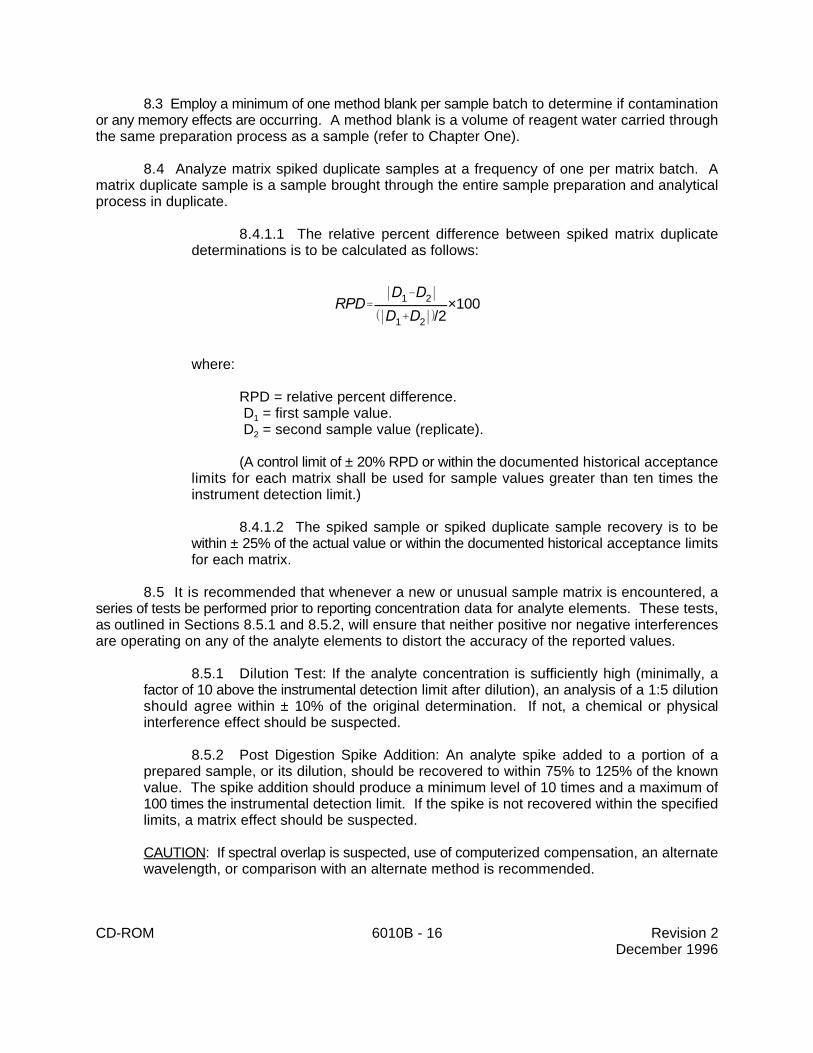
8.4.1.1 The relative percent difference between spiked matrix duplicatedeterminations is to be calculated as follows:
where:
RPD = relative percent difference. D = first sample value.1
D = second sample value (replicate).2
(A control limit of ± 20% RPD or within the documented historical acceptancelimits for each matrix shall be used for sample values greater than ten times theinstrument detection limit.)
8.4.1.2 The spiked sample or spiked duplicate sample recovery is to bewithin ± 25% of the actual value or within the documented historical acceptance limitsfor each matrix.
8.5 It is recommended that whenever a new or unusual sample matrix is encountered, aseries of tests be performed prior to reporting concentration data for analyte elements. These tests,as outlined in Sections 8.5.1 and 8.5.2, will ensure that neither positive nor negative interferencesare operating on any of the analyte elements to distort the accuracy of the reported values.
8.5.1 Dilution Test: If the analyte concentration is sufficiently high (minimally, afactor of 10 above the instrumental detection limit after dilution), an analysis of a 1:5 dilutionshould agree within ± 10% of the original determination. If not, a chemical or physicalinterference effect should be suspected.
8.5.2 Post Digestion Spike Addition: An analyte spike added to a portion of aprepared sample, or its dilution, should be recovered to within 75% to 125% of the knownvalue. The spike addition should produce a minimum level of 10 times and a maximum of100 times the instrumental detection limit. If the spike is not recovered within the specifiedlimits, a matrix effect should be suspected.
CAUTION: If spectral overlap is suspected, use of computerized compensation, an alternatewavelength, or comparison with an alternate method is recommended.
CD-ROM 6010B - 17 Revision 2December 1996
8.6 Check the instrument standardization by analyzing appropriate QC samples as follows.
8.6.1 Verify calibration with the Continuing Calibration Verification (CCV) Standardimmediately following daily calibration, after every ten samples, and at the end of ananalytical run. Check calibration with an ICV following the initial calibration (Section 5.6).At the laboratory’s discretion, an ICV may be used in lieu of the continuing calibrationverifications. If used in this manner, the ICV should be at a concentration near the mid-pointof the calibration curve. Use a calibration blank (Section 5.5.1) immediately following dailycalibration, after every 10 samples and at the end of the analytical run.
8.6.1.1 The results of the ICV and CCVs are to agree within 10% of theexpected value; if not, terminate the analysis, correct the problem, and recalibrate theinstrument.
8.6.1.2 The results of the check standard are to agree within 10% of theexpected value; if not, terminate the analysis, correct the problem, and recalibrate theinstrument.
8.6.1.3 The results of the calibration blank are to agree within three times theIDL. If not, repeat the analysis two more times and average the results. If theaverage is not within three standard deviations of the background mean, terminatethe analysis, correct the problem, recalibrate, and reanalyze the previous 10samples. If the blank is less than 1/10 the concentration of the action level ofinterest, and no sample is within ten percent of the action limit, analyses need not bererun and recalibration need not be performed before continuation of the run.
8.6.2 Verify the interelement and background correction factors at the beginningof each analytical run. Do this by analyzing the interference check sample (Section 5.8).Results should be within ± 20% of the true value.
9.0 METHOD PERFORMANCE
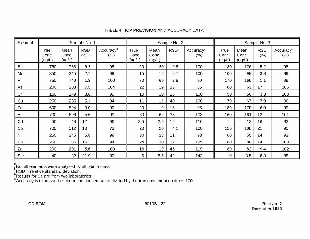
9.1 In an EPA round-robin Phase 1 study, seven laboratories applied the ICP techniqueto acid-distilled water matrices that had been spiked with various metal concentrates. Table 4 liststhe true values, the mean reported values, and the mean percent relative standard deviations.
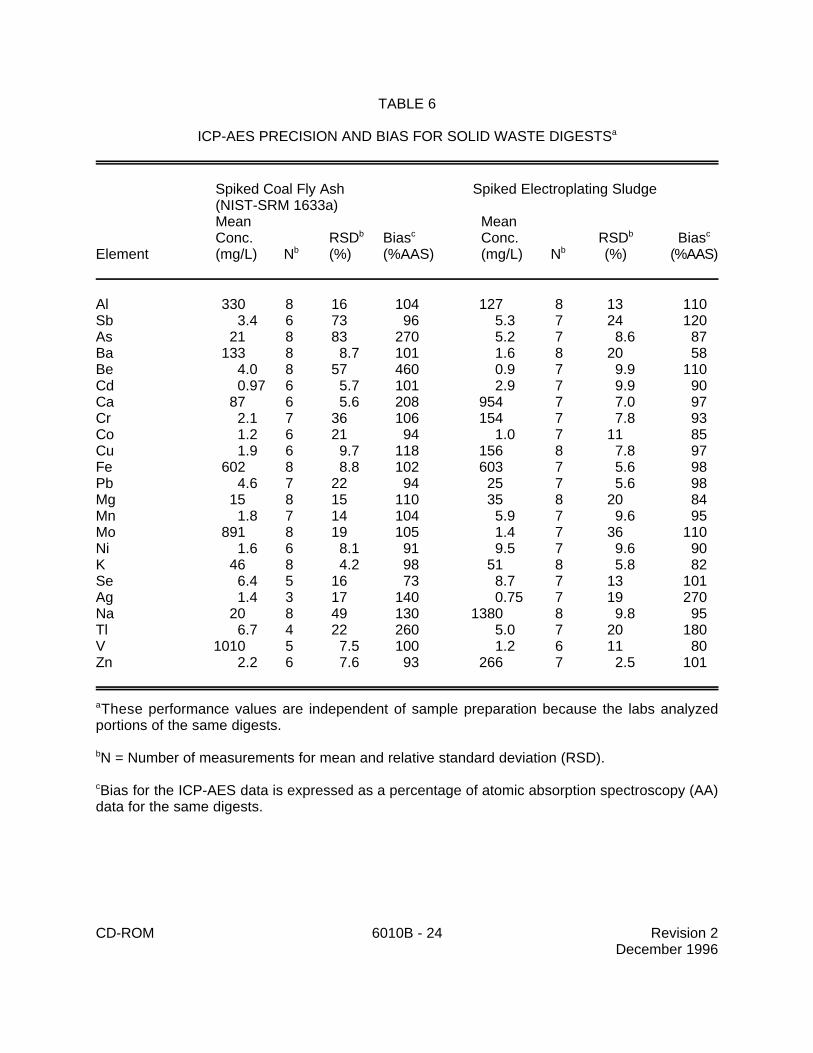
9.2 Performance data for aqueous solutions and solid samples from a multilaboratorystudy (9) are provided in Tables 5 and 6.
10.0 REFERENCES
1. Boumans, P.W.J.M. Line Coincidence Tables for Inductively Coupled Plasma AtomicEmission Spectrometry, 2nd Edition. Pergamon Press, Oxford, United Kingdom, 1984.
2. Sampling and Analysis Methods for Hazardous Waste Combustion; U.S. EnvironmentalProtection Agency; Air and Energy Engineering Research Laboratory, Office of Research andDevelopment: Research Triangle Park, NC, 1984; Prepared by Arthur D. Little, Inc.
CD-ROM 6010B - 18 Revision 2December 1996
3. Rohrbough, W.G.; et al. Reagent Chemicals, American Chemical Society Specifications, 7thed.; American Chemical Society: Washington, DC, 1986.
4. 1985 Annual Book of ASTM Standards, Vol. 11.01; "Standard Specification for ReagentWater"; ASTM: Philadelphia, PA, 1985; D1193-77.
5. Jones, C.L. et al. An Interlaboratory Study of Inductively Coupled Plasma Atomic EmissionSpectroscopy Method 6010 and Digestion Method 3050. EPA-600/4-87-032, U.S. EnvironmentalProtection Agency, Las Vegas, Nevada, 1987.
CD-ROM 6010B - 19 Revision 2December 1996
TABLE 1RECOMMENDED WAVELENGTHS AND ESTIMATED INSTRUMENTAL DETECTION LIMITS
The wavelengths listed (where x2 indicates second order) are recommended because ofa
their sensitivity and overall acceptance. Other wavelengths may be substituted (e.g., in the case ofan interference) if they can provide the needed sensitivity and are treated with the same correctivetechniques for spectral interference (see Section 3.1). In time, other elements may be added asmore information becomes available and as required.
The estimated instrumental detection limits shown are provided as a guide for anb
instrumental limit. The actual method detection limits are sample dependent and may vary as thesample matrix varies.
Highly dependent on operating conditions and plasma position.c
CD-ROM 6010B - 20 Revision 2December 1996
TABLE 2POTENTIAL INTERFERENCES
ANALYTE CONCENTRATION EQUIVALENTS ARISING FROMINTERFERENCE AT THE 100-mg/L LEVEL
c
Interferanta,b
Wavelength ---------------------------------------------------------------------------------------------- Analyte (nm) Al Ca Cr Cu Fe Mg Mn Ni Ti V
Dashes indicate that no interference was observed even when interferents were introduced at thea
following levels: Al - 1000 mg/L Mg - 1000 mg/L Ca - 1000 mg/L Mn - 200 mg/L Cr - 200 mg/L Tl - 200 mg/L Cu - 200 mg/L V - 200 mg/L Fe - 1000 mg/L
The figures recorded as analyte concentrations are not the actual observed concentrations; to obtainb
those figures, add the listed concentration to the interferant figure.Interferences will be affected by background choice and other interferences may be present.
c
CD-ROM 6010B - 21 Revision 2December 1996
TABLE 3MIXED STANDARD SOLUTIONS
Solution Elements
I Be, Cd, Mn, Pb, Se and Zn II Ba, Co, Cu, Fe, and V III As, Mo IV Al, Ca, Cr, K, Na, Ni,Li, and Sr V Ag (see “NOTE” to Section 5.4), Mg, Sb, and Tl VI P
CD-ROM 6010B - 22 Revision 2December 1996
TABLE 4. ICP PRECISION AND ACCURACY DATAa
Element Sample No. 1 Sample No. 2 Sample No. 3
True Mean RSD Accuracy True Mean RSD Accuracy True Mean RSD AccuracyConc. Conc. (%) (%) Conc. Conc. (%) Conc. Conc. (%) (%)(ug/L) (ug/L) (ug/L) (ug/L) (ug/L) (ug/L)
b d b d b d
Be 750 733 6.2 98 20 20 9.8 100 180 176 5.2 98
Mn 350 345 2.7 99 15 15 6.7 100 100 99 3.3 99
V 750 749 1.8 100 70 69 2.9 99 170 169 1.1 99
As 200 208 7.5 104 22 19 23 86 60 63 17 105
Cr 150 149 3.8 99 10 10 18 100 50 50 3.3 100
Cu 250 235 5.1 94 11 11 40 100 70 67 7.9 96
Fe 600 594 3.0 99 20 19 15 95 180 178 6.0 99
Al 700 696 5.6 99 60 62 33 103 160 161 13 101
Cd 50 48 12 96 2.5 2.9 16 116 14 13 16 93
Co 700 512 10 73 20 20 4.1 100 120 108 21 90
Ni 250 245 5.8 98 30 28 11 93 60 55 14 92
Pb 250 236 16 94 24 30 32 125 80 80 14 100
Zn 200 201 5.6 100 16 19 45 119 80 82 9.4 102
Se 40 32 21.9 80 6 8.5 42 142 10 8.5 8.3 85c
Not all elements were analyzed by all laboratories.a
RSD = relative standard deviation.b
Results for Se are from two laboratories.c
Accuracy is expressed as the mean concentration divided by the true concentration times 100.d
CD-ROM 6010B - 23 Revision 2December 1996
TABLE 5
ICP-AES PRECISION AND ACCURACY FOR AQUEOUS SOLUTIONSa