46
1 Methodology for Establishing Baseline Scenarios in the Urban Water Sector with ECAM

1
Methodology for Establishing Baseline Scenarios
in the Urban Water Sector with ECAM

2
IUWA - Institut für Umweltwirtschaftsanalysen Heidelberg e.V. Sha Xia ∙ Michael Seyboth ∙ Kevin Fleckenstein ∙ Sophie Gindele
Water and Wastewater Companies for Climate Mitigation – WaCCliM Adriana Noelia Veizaga Campero ∙ Elaine Cheung
3
Table of Contents
List of Figures ............................................................................................................................................................................................ 4
List of Tables .............................................................................................................................................................................................. 4
List of Abbreviations ................................................................................................................................................................................. 5
Summary ..................................................................................................................................................................................................... 6
Introduction ................................................................................................................................................................................................ 8
Baseline emission scenarios ..................................................................................................................................................................... 9
Methodology development .................................................................................................................................................................... 11
Step 1: System boundaries & time horizon .......................................................................................................................................... 13
1.1. System boundary of the urban water cycle ..............................................................................................................................................13
1.2. Pathways of GHG emissions in the urban water cycle ........................................................................................................................14
1.3. Time horizon ........................................................................................................................................................................................................15
Step 2: Analysis of driving factors and key parameters ..................................................................................................................... 17
2.1. Key parameters ...................................................................................................................................................................................................17
2.2. Driving factors behind key parameters ......................................................................................................................................................17
2.3. Values and trends for projecting ECAM inputs ........................................................................................................................................20
2.3.1. Resident population ...........................................................................................................................................................................21
2.3.2. Population with access to water and sanitation services .....................................................................................................21
2.3.3. Water and wastewater volume .......................................................................................................................................................23
2.3.4. Billed authorised consumption volume ......................................................................................................................................24
2.3.5. Energy consumption ...........................................................................................................................................................................24
2.3.6. Energy costs ...........................................................................................................................................................................................25
2.3.7. Emission factor for grid electricity ................................................................................................................................................26
2.3.8. Protein generation per capita per year ........................................................................................................................................26
2.3.9. BOD5 generation per capita per year ............................................................................................................................................26
2.3.10. CH4 emission factors ...........................................................................................................................................................................26
2.3.11. BOD5 loads .............................................................................................................................................................................................26
2.3.12. Nitrogen concentration in the effluent .......................................................................................................................................27
Step 3: Data collection & projection ..................................................................................................................................................... 29
Step 4: GHG analysis as BAU scenarios using ECAM ........................................................................................................................... 31
Bibliography ............................................................................................................................................................................................. 33
Annex A Overview of all GHG emissions from water and wastewater services .............................................................................. 36
Annex B Analysis of key parameters shaping baseline GHG emissions in the urban water cycle ................................................. 37
Annex C Overview of parameters and ECAM inputs ........................................................................................................................... 40
Annex D Projection of nitrogen concentration in the effluent ........................................................................................................ 43
Annex E Statistical methods for calculating average growth rates ................................................................................................. 44

4
List of Figures
Figure 1. Steps to develop BAU scenarios ...................................................................................................................................................................11
Figure 2. System boundary. ...............................................................................................................................................................................................13
Figure 3. Driving factors affecting key parameters ..................................................................................................................................................17
Figure 4. Typical energy intensity for various processes in the water and wastewater sector ...............................................................25
Figure 5. The process chain of the guideline, PEIGE tool, and ECAM tool. .....................................................................................................31
List of Tables
Table 1. ECAM and PEIGE inputs of the resident population (PO-01, PO-02). ..............................................................................................21
Table 2. Population groups with different infrastructure access used in sub-stages and the associated ratios in total residents. .............................................................................................................................................................................................................22
Table 3. PEIGE inputs of the volume of billed authorised consumption (W-07). ..........................................................................................23
Table 4. The water and wastewater volume used in sub-stages and the per capita terms. .....................................................................23
Table 5. The allocation of the energy consumption quantity to water/wastewater volume and energy intensity in sub-stages. ................................................................................................................................................................................................................................25
Table 6. ECAM and PEIGE inputs of the electricity price, emission factor for grid electricity and protein generation per capita per year (EC-01, CF-01, CF-02). ...................................................................................................................................................................26
Table 7. PEIGE and ECAM inputs related to BOD5 and nitrogen load ...............................................................................................................27

5
List of Abbreviations
2030 WRG 2030 Water Resources Group
BAU Business-as-usual
BMU [GER] Federal Ministry for the Environment, Nature Conservation and Nuclear Safety
BOD Biochemical Oxygen Demand
CAGR Compound Annual Growth Rate
CH4 Methane
CO2 Carbon dioxide
ECAM Energy Performance and Carbon Emissions Assessment and Monitoring
EDGAR [EU] Emissions Database for Global Atmospheric Research
EF Emission Factor
EPA [US] Environmental Protection Agency
GHG Greenhouse Gas
GWh Gigawatt-hours
GWP Global Warming Potential
IBNET International Benchmarking Network for Water and Sanitation Utilities
IEA International Energy Agency
IKI International Climate Initiative
IMF International Monetary Fund
IPCC Intergovernmental Panel on Climate Change
IWA International Water Association
JMP Joint Monitoring Programme for Water Supply, Sanitation and Hygiene
kWh kilowatt-hour
MRV Measuring, Reporting, and Verification
Mtoe Million tonnes of oil equivalent
N2O Nitrous oxide
NEPCO [JOR] National Electric Power Company
NRW Non-Revenue Water
OECD Organisation for Economic Co-operation and Development
PEIGE Tool of Projecting ECAM Inputs for GHG Emissions as BAU Scenarios
PPI Producer Price Index
SDG Sustainable Development Goal
TN Total Nitrogen
TOW Total Organics in Wastewater
TWh Terawatt-hours
UN United Nations
UNDESA United Nations Department of Economic and Social Affairs
UNDP United Nations Development Programme
UNESCAP United Nationations Economic and Social Commission for Asia and the Pacific
UNICEF United Nations Children’s Fund
UNSD United Nations Statistics Division
WaCCliM Water and Wastewater Companies for Climate Mitigation
WASH drinking water, sanitation and hygiene
WHO World Health Organisation
WWAP World Water Assessment Programme
WWTP Wastewater Treatment Plant
WWU Water and Wastewater Utility
6
Summary
Climate change poses significant risks to the water and wastewater services provided in human settlements. At the same time, these also hold enormous potential for mitigat-ing climate change. As water is transferred across the urban water cycle to meet the various demands of society, green-house gas (GHG) emissions are released directly during the biological degradation of organics in wastewater and indi-rectly through energy consumption. With the aim of enabling companies, institutions and government agencies to identify reduction potentials, this methodology outlines the path for establishing the business-as-usual (BAU) emission scenarios water and wastewater utilities could exhibit in the mid-term if the current management and practices were to continue.
Based on the physical and biochemical characteristics of the emission pathways in the urban water cycle, key parameters can be identified that determine the direction and magni-tude of the variation of GHG emissions. They are primarily the parameters associated with the range of anthropogenic activities that release the emissions. Impacted by various so-cio-economic and technological drivers, these parameters evolve over time and can be projected based on the trend derived from studies of international and national databases, journal papers, reports and policy documents, which are pre-sented in this methodology.
The approach is created on the basis of the “Energy Perfor-mance and Carbon Emissions Assessment and Monitoring” (ECAM) tool of the international project “Water and Wastewater Companies for Climate Mitigation (WaCCliM)”. Based on the projected future values of the key parameters, the variables that are necessary to be inputted into ECAM – the ECAM inputs – for the computation of GHG emissions can be quantified for a certain point of time. This step will be facilitated by the “Tool of Projecting ECAM Inputs for GHG Emissions as BAU Scenarios (PEIGE)” in Excel format, which automatically calculates future values once users have en-tered the required input values.
Applying the established modelling for BAU scenario projec-tions, the pilot utilities of the WaCCliM project demonstrate various aspects of mitigation potentials. The optimisation of energy efficiency and biogas recovery, the promotion of wa-ter conservation and the improvement of the wastewater services in the quantity and quality are associated with the most substantial benefits in terms of mitigating climate risks, improving financial performance and implementing the Sustainable Development Goals.

7
Introduction
©Sh
utte
rsto
ck

8
Introduction
The water sector is facing enormous challenges. To satisfy soaring demands from the growing number of inhabitants and economic activities, the water industry in many coun-tries is struggling with declining water availability. The pres-sure caused by population growth, urbanisation, and industrialisation is exacerbated by the various impacts of cli-mate change, which are increasingly observed across the globe [IPCC, 2014a].
At the same time, water and wastewater utilities (WWUs) are also contributors to climate change, estimated to be respon-sible for 3%-7% of a country’s total greenhouse gas (GHG) emissions [IWA, 2015]. In light of stronger water consump-tion needs in the future, continuing the present trajectory will push the emission level even higher, aggravating the magnitude of expected climate impacts and water stress.
As a guideline for water professionals and decision-makers, this document shall illustrate the steps to establish baseline scenarios of GHG emission development in the urban water cycle, which would arise in the future if no action was taken. The approach is created on the basis of the version 2.2 of the “Energy Performance and Carbon Emissions Assessment and Monitoring” (ECAM) tool of the international project “Water and Wastewater Companies for Climate Mitigation (WaCCliM)“, funded through the International Climate Initia-tive (IKI) of the German Federal Ministry for the Environment, Nature Conservation and Nuclear Safety (BMU).
As the very first of its kind, ECAM allows for a holistic ap-proach of the urban water cycle to drive GHG emission re-duction in utilities, even those with limited data availability. It is designed to assess the carbon emissions that WWUs can control and prepares them for future reporting needs for cli-mate mitigation.
Using the ECAM tool, this methodology takes a further step in developing the capabilities of GHG measuring, reporting, and verification (MRV). By identifying the evolution of GHG emissions in the business-as-usual (BAU) condition, it facili-tates the exploration of reduction potentials as well as the evaluation of the success of mitigation efforts.
To achieve these objectives, the methodology is organised in simple steps as follows:
• Step 1 outlines the framework of the study, including the examined system of the urban water cycle, the rel-evant GHGs and their emission pathways.
• Step 2 analyses the driving factors behind the key pa-rameters determining the direction and scope of the de-velopment of baseline emissions in the system considered.
• Step 3 describes the collection of data and the projec-tion of the key ECAM inputs based on the effects of driv-ing factors.
• Step 4 explains the calculation pathways of BAU emis-sion scenarios with the ECAM tool.
The approaches quantifying GHG emissions embedded in the ECAM tool and this document are developed in accordance with the 2006 Guidelines for National GHG Inventions of the Intergovernmental Panel on Climate Change (IPCC) [2006].

9
Baseline emission scenarios
A baseline scenario related to GHG emissions is a reference situation describing an actual or assumed future trajectory of the evolution of GHG emissions in the absence of climate change abatement actions. It shows the level of emissions in the coming decades without intervention measures specifi-cally addressing climate change. Baseline scenarios are es-tablished to identify emission reduction potentials of a particular action and the associated costs.
Baseline scenarios are developed under various assumptions of demographic and macroeconomic change, technological development and penetration, resource intensity, climate change impacts and many other aspects. Depending on the assumptions about future events in these areas, the results of baseline scenario concepts could deviate greatly from each other. According to the IPCC [2001], the literature dif-ferentiates between several concepts of baselines, including:
• Business-as-usual (BAU) baseline, which assumes that future development trends follow those of the past – i.e. the “no policy change” scenario
• Efficient baseline, which implies the efficient utilisation of all resources
The occurrence of the efficient baseline has the prerequisite of adequately functioning markets that internalise environ-mental costs to promote the wide-ranging dissemination and application of efficiency-enhancing technologies. This condition is not usually fulfilled in developing and emerging countries, meaning that such techniques are often combined with high investment and operation costs and are not fa-voured on a large scale [IPCC, 2001]. As such, this method-ology applies the concept of BAU scenarios for the estimation of the annual GHG emissions in the urban water cycle.

10
Methodology development
©Ra
cool
_stu
dio
/ Fre
epik

11
1 2 3 4
Definition of system
boundaries and time horizon
Identification of key parameters
and driving factors
Data collection & projection
Development of BAU
scenarios using ECAM
Methodology development
Step 1: Definition of boundaries and time horizon
In order to explore the future quantity of GHGs released in the urban water cycle as baselines, the first step is to identify the fundamental framework within which the envisaged methodology is developed. To fulfil this task, this step sets the boundary and elements of the urban water cycle consid-ered in this study. Sources and pathways of GHG emissions released in the system, mainly carbon dioxide (CO2), me-thane (CH4) and nitrous oxide (N2O), will be then briefly out-lined. Finally, the option and time horizon adopted for baseline scenarios must be defined.
Step 2: Identification of the key parameters and driving factors that affect the GHG emission trajec-tory
To establish baseline scenarios in the urban water cycle, it is necessary to track the essential terms that evolve and char-acterise the tendency and magnitude of GHG emission vari-ations. These are primarily the parameters associated with the range of anthropogenic activities that release the emis-sions. In this step, the key parameters and the driving factors
behind the key parameters will be introduced and analysed in the context of the global trend. This step varies and ad-justs according to each local context and the time frame de-cided for the scenario establishment.
Step 3: Data collection & projection
Data must be collected preferably from water utilities. To fa-cilitate this step, a tool to Project ECAM Inputs for GHG Emis-sions as BAU Scenarios (PEIGE) was developed, which projects data based on fixed BAU trends analysed in step 2, nevertheless, the tool should be adjusted and fit to local or utility BAU trends.
Step 4: Development of BAU scenarios using ECAM
Once the data are projected, these will be the input source in ECAM to determine the GHG emissions in any desired time frame. This will then outline the trajectory of GHG emissions to be considered as the BAU scenario.
Figure 1. Steps to develop BAU scenarios

12
Step 1: System boundaries & time horizon
13
Step 1: System boundaries & time horizon
1.1. System boundary of the urban wa-ter cycle
Water moves through the natural hydrologic cycle in the Earth’s physical system. In human settlements, water is used intensively to meet the diversified demands of society. Being significantly modified by anthropogenic impacts, water cir-culation in urban areas covers a broad scope of pathways and components within the natural and human systems as well as between the two [Marsalek et al., 2006].
In studies about anthropogenic GHG emissions resulting from the urban water cycle, the part of human-dominated water circulation is of central interest. It includes water sup-ply, drainage, wastewater collection and management, as well as the beneficial uses of receiving waters [Marsalek et al., 2006].
1 In the context of public water and wastewater services, domestic water/wastewater and municipal water/wastewater are the most widely used terms that are comparable to each other in many cases. Domestic water/wastewater refers to services supplied to households for drinking, cooking, cleaning, and sanitation. Municipal water/wastewater includes all that is connected to the public distribution network, including households, shops, services, some urban industries, some urban agriculture, etc. FAO (2016), glossary.
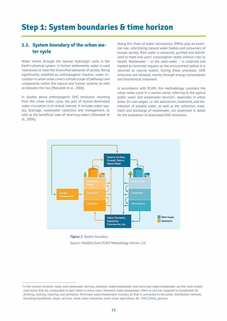
Along this chain of water conveyance, WWUs play an essen-tial role, interlinking natural water bodies and consumers of human society. Raw water is extracted, purified and distrib-uted to meet end-users’ consumption needs without risks to health. Wastewater – or the used water – is collected and treated to minimise impacts on the environment before it is returned to natural waters. During these processes, GHG emissions are released, mainly through energy consumption and biochemical treatment.
In accordance with ECAM, this methodology considers the urban water cycle in a narrow sense, referring to the typical public water and wastewater services1, especially in urban areas. Six sub-stages, i.e. the abstraction, treatment, and dis-tribution of potable water, as well as the collection, treat-ment and discharge of wastewater, are examined in detail for the evaluation of associated GHG emissions.
Figure 2. System boundary.
Source: Modified from ECAM Methodology Version 2.0.

14
1.2. Pathways of GHG emissions in the urban water cycle
The main GHGs emitted in the urban water cycle include CO2, CH4, and N2O. Compared regarding the global warming po-tentials (GWP)2 over the 100-year horizon, CO2 accounts for the majority of the overall GHG emissions from the urban water cycle. However, CH4 and N2O also contribute signifi-cantly due to their high GWP of 34 and 298 CO2-equivalents respectively [IPCC, 2014a], although they are released in a much smaller quantity. Whereas CO2 emissions are all at-tributed to energy consumption, CH4 and N2O emissions are produced primarily during biological processes in the wastewater section. Therefore, the pathways of GHG emis-sions in the urban water cycle can be divided into energy-related and non energy-related sources.
Energy-related emissions
Energy consumption is a significant source of GHG emissions in the urban water cycle. Energy is necessary for WWUs to empower their facilities, especially for pumping and treat-ment. The associated fossil fuel combustion results in indi-rect or direct emissions of GHGs, mainly CO2, depending on whether the energy is transmitted from the public electricity grid or generated by on-site engines. In those WWUs where water distribution and wastewater discharge take place by truck transport instead of by pipelines and drainage net-works, emissions are released through fossil fuel combustion of vehicles. If the distribution and discharge are accom-plished via gravity, no energy is needed. For better focusing, this methodology concentrates on energy-related emissions resulting from electricity consumption.
According to the International Energy Agency (IEA) [2016c], the global water and wastewater sector, including serving households, agriculture and industry, consumed around 120 million tonnes of oil equivalent (Mtoe) in 2014. 60% was at-tributed to electricity, equalling 820 terawatt-hours (TWh), or around 4% of the global electricity demand. The electric power was mainly consumed for water extraction (40%), wastewater collection and treatment (25%), and water dis-tribution (20%). Moreover, there is an apparent disparity be-tween low/middle-income and high-income countries: 42% of the water-related electricity was used for wastewater treatment in industrialised nations, whereas the share was much smaller in developing and emerging economies due to the lower degree of wastewater treatment.
2 The GWP is defined as the time-integrated, normally 100 years, radiative forcing from the emission of a given gas, relative to that of an equal mass of CO2. It is the most commonly used emission parameter to compare different GHGs and has become the default metric for transferring the emissions of gases to CO2 equivalent emissions (CO2e). IPCC (2014a).
Non-energy related emissions
Non-energy related emissions are primarily CH4 and N2O, which are produced during the collection, treatment and dis-charge of wastewater. According to the EU Emissions Data-base for Global Atmospheric Research (EDGAR), the wastewater sector, including treated and untreated sewage from all sources, contributes approximately 11% of the total global methane release as well as 4% of global N2O emis-sions [Janssens-Maenhout et al., 2017; JRC & PBL, 2016].
In wastewater treatment plants (WWTPs), methane is emit-ted through the anaerobic decomposition of organic mate-rial. The anaerobic digestion of the primary sludge may be a substantial emitting source if the emitted CH4 is not flared or recovered. N2O emissions are associated with the degra-dation of nitrogen components through microbial processes such as nitrification and denitrification, which takes place in sewers and treatment plants as well as in discharged efflu-ents. Both gases can be further emitted in the handling and disposal of digested sludge, which is, however, not consid-ered in the present document. Also excluded from the as-sessment are the CH4 and N2O emissions in sewers due to the deficiency of appropriate methodologies according to the IPCC. Moreover, CO2 emissions from biological wastewater treatment are not examined, either, as they are defined as biogenic and not considered in the IPCC 2006 Guidelines.
In countries with inadequate infrastructure, the use or dis-charge of untreated wastewater can lead to significant CH4 and N2O emissions and adverse impacts on public health and the environment. Due to the possibility to convert methane to valuable energy, tackling untreated wastewater can real-ise remarkable potentials of climate mitigation and the im-provement of utilities’ energy and operation security. To highlight the possibilities, ECAM and the present methodol-ogy also examine these uncontrolled emissions, despite their being produced partly outside the boundary of WWUs.
The ECAM tool categorises the emission pathways described above into three scopes consistent with the IPCC standard. Scope 1 summarises all direct emissions from sources that are owned or controlled by the WWUs. Scope 2 refers to in-direct emissions owing to the generation of purchased elec-tricity consumed by the WWUs. Scope 3 covers other indirect emissions released as consequences of the activities of the WWUs, but from sources not owned or controlled by them. Annex A presents an overview of GHG emissions considered in this guideline.

15
1.3. Time horizon
For the establishment of baselines, the IPCC [2001] sees a general difficulty in predicting a development pattern over the long term due to the lack of knowledge about the dy-namic linkages between technical choices and consumption patterns. These two factors interact with economic signals and policies, affecting the validity of baseline assumptions. Further uncertainties for long-term scenarios arise from po-tential political and social changes, which are primarily the case in developing countries and emerging economies amid massive urbanisation and industrialisation processes.
Apart from the above considerations, this document does not examine the carrying capacity of local water resources that limit the infinite expansion of human settlements in the long term. To do so, sophisticated hydrological modelling is re-quired. Therefore, this methodology focuses on baselines of near to mid-term, up to about two decades ahead.

16
©Sh
utte
rsto
ck
©Sh
utte
rsto
ck
©Sh
utte
rsto
ck
©Sh
utte
rsto
ck
Step 2: Analysis of driving factors and key parameters
Step 2: Analysis of driving factors and key parameters
Step 2: Analysis of driving factors and key parameters
Step 2: Analysis of driving factors and key parameters

17
Population growth and
urbanisation
Consumption behaviour and income devel-
opment Water stress and impacts
of climate change
Energy generation technology
Water-energy nexus
in the urban water cycle
Energy and water prices
Key parameters
Step 2: Analysis of driving factors and key parameters
2.1. Key parameters
Based on the characteristics of GHGs and their emission pathways, the IPCC Guideline [2006] set standards for meas-uring emissions depending on various parameters and vari-ables. To establish baseline scenarios in the urban water cycle, it is necessary to track the essential terms that evolve and characterise the tendency and magnitude of GHG emis-sion variations. These are primarily the parameters associ-ated with the range of anthropogenic activities that release the emissions. As such, an extensive analysis, as presented in Annex B, reveals that the development of the categories of key parameters will affect the future trajectory of GHG emissions in the urban water cycle.
In the present methodology, the group of key parameters re-fers to those for which future rates of change in BAU scenar-ios will be studied in this document. These parameters determine the variation range of other variables and total GHG emissions. As already summarised previously, key pa-rameters include:
1. Resident population in the service area 2. Connection degree of water and sanitation infrastruc-
tures 3. Per capita water production and wastewater volume 4. Energy intensity per volume of water and wastewater 5. Emission factor of grid electricity 6. Per capita per day BOD5 generation quantity 7. Per capita per day protein consumption quantity.
Apart from GHG emissions, this methodology also investi-gates the development of energy costs. Thus, the energy price is also seen as one of the key parameters, for which the analysis of the future trend is needed. Moreover, due to the vast potential to improve the water efficiency in low- and middle-income countries, the changes in the non-revenue water (NRW) ratio in the pilot countries are also projected based on the past trend. Thus, the group of key parameters also include:
8. Energy price 9. Non-revenue water.
2.2. Driving factors behind key parame-ters
The future values of key parameters are posed as the results of alterations of human activities, responding to socio-eco-nomic, environmental and technical drivers. Here, the driv-ing factors behind the key parameters will be introduced and analysed in the context of the global trend.
Figure 3. Driving factors affecting key parameters
Population growth and urbanisation
Population growth is the most important driving factor of GHG emissions in the water and wastewater sector, affecting the amount of water production and wastewater generation as well as BOD5 and nitrogen load in the sewage.
The expansion of the human population has accelerated dra-matically. Between 1900 and 2000, the total population has grown from 1.5 to 6.1 billion at a pace three times faster than during the entire previous history [Roser & Ortiz-Ospina, 2018]. Currently, 7.6 billion people live on Earth. By 2050, this number is estimated to hit 9.8 billion, and 11.2 billion in 2100 [UNDESA, 2017a].
The exponentially growing population poses a significant challenge to the carrying capacity of our planet. Water, with its essential role for life and economic activities, is particularly affected. Over the last several decades, the growth rate of wa-ter demand has doubled that of the population. At the same time, the inter-sectoral competition for water use has been in-tensified [WWAP, 2015]. Currently, about 80% of inhabitants

18
worldwide live in areas where water security3 is threatened [Vörösmarty et al., 2010]. With the further growth of the pop-ulation, the global water demand is expected to be 55% higher in 2050 [OECD, 2012], while the water deficit is pro-jected to increase 40% by 2030 [2030 WRG, 2009].
Today, 50% of the global population resides in cities, and this share will reach 70% by 2050. The urbanisation process, which is taking place primarily in low- and middle-income countries, generates specific and localised pressures on wa-ter and its management practices. In urban areas of these nations, where the slum population is rapidly expanding, the water supply, sanitation and hygiene services are often in-adequate, posing a threat to human health, the environment and economic development. Investments in water and sani-tation infrastructures result in considerable gains through protecting urban living conditions and securing economic activities. Additional financial benefits can be created by em-ploying the productive potential of wastewater as a resource for energy and nutrients, as well as for other sectors such as agriculture [WWAP, 2015].
Consumption behaviour and income development
Consumption behaviour plays a role in several key parame-ters of the baseline projection, including per capita water consumption, BOD5 generation and protein intake. Variations of consumer behaviour in developing countries and emerg-ing markets are often driven by higher income accompanied by urbanisation, which changes the style and standard of liv-ing over time.
In urban areas, the expanding middle class have notably contributed to shifts towards more water-intensive con-sumption patterns, such as using more piped water on prem-ises, dishwashers, washing machines, flushing toilets and showers. People also tend to build larger houses, eat more meat, drive more motor vehicles and use other energy-con-suming devices. As a consequence, water uses for both pro-duction and domestic purposes has sharply increased [WWAP, 2015]. However, the relation between income and per capita water consumption, especially that for domestic uses, is not necessarily linear. According to the UN [WWAP, 2014], residents consume less water per person after reach-ing a certain income level. Reasons behind this include the adoption of more water-saving appliances and measures in homes, reduction of water losses including leakage from wa-ter distribution systems and growing awareness among con-sumers.
The personal BOD generation is also positively linked to eco-nomic wealth. Higher living standards lead to improved san-itary conditions and dietary consumption, which intensify organic contamination of water and thus increase the BOD load. Currently, the default values for BOD5 generation adopted in the IPCC Guideline [2006] are generally higher
3 The United Nations (UN) define water security as the capacity to safeguard sustainable access to adequate quantities of acceptable quality water. UN, (2013), p.1.
4 Individual food consumption preferences also vary, for instance if the family size and composition, place of residence, health situation or season of the year changes. Further possible influencing factors include education level, occupation, urbanisation and globalisation. Tim-mer, et al. (1983); Rampal (2018).
for industrialised countries than for developing countries and emerging economies. However, the income level is not the only determining factor, and regional differences can be caused due to other socio-economic factors such as life-styles, habits and technical features [Doorn & Liles, 1999; Henze & Comeau, 2008].
Protein consumption is also dependent on consumer behav-iour. Diversified food commodities provide protein, with an-imal products containing higher protein content. Meanwhile, the different positions in the food chain make the animal protein more costly per unit weight than that from other sources [Grigg, 1995]. The amount of protein intake is, there-fore, an issue of consumers’ choices about food consumption pattern determined by their income, food prices and fa-voured tastes.4 According to Henchion et al. [2017] and the Organisation for Economic Co-operation and Development and Food and Agriculture Organisation (FAO) [2015, 2018], income growth and urbanisation are the two primary drivers of general food consumption, promoting the diversification of the nutrition pattern towards more protein intake – espe-cially from animal sources – in the developing world. More-over, taste differences translate higher income into higher consumption of different food products, also contributing to regional variations in protein intake.
Generally, there are multiple reasons for changes in con-sumer behaviour, the quantification of the interrelations of-ten requiring empirical investigations.
Water stress and impacts of climate change
Currently, alterations in both the quantity and quality of re-gional and global water resources are taking place due to climate change [IPCC, 2014b]. Most extreme events are char-acterised by the absence of or high quantities of water as the result of intensified water circulation [EPA, 2016; IPCC, 2014a]. Consequently, the regional and seasonal contrast in water resources is exaggerated: dry regions and seasons get drier, while wet regions and seasons become more humid. The increase in water temperature, low flows and heavy rain-fall pose a further threat to the quality of water resources through pollutants including sediments, nutrients, patho-gens and pesticides [Jiménez Cisneros et al., 2014; Kundze-wicz et al., 2007].
Due to the essential role of water, hydrological changes lead to the most widespread impacts on human society. Municipal water services and infrastructure are considerably affected. Apart from the increased water demand and intensified com-petition with other sectors, further possible consequences for water supply are, for instance, the need for more exten-sive water storage due to river flow shifts and droughts, en-hanced treatment requirements due to higher pollutants burden in raw water, and higher desalination needs in coastal regions. In the case of wastewater, three possible
19
scenarios can occur: Wet weather causes higher amounts of rainfall that exceeds the design range and puts pressure on combined canal systems; Dry weather leads to cracking sew-ers and more infiltration and exfiltration of water and wastewater, increasing corrosion of sewers and maintenance costs; Rising sea levels lead to higher amounts of salty water affecting sewer systems. In both wet and dry conditions, greater pollutant and pathogen content is expected in wastewater [Jiménez Cisneros et al., 2014]. All of these is-sues will significantly increase energy consumption and op-erational and investment costs, as well as GHG emissions.
To address the upcoming challenges, municipal water man-agement in the developing world shall be prepared as soon as possible. Substantial and sustained emission reductions in the near term reduce future challenges and costs signifi-cantly and increase the overall effectiveness of adaptation measures. Strategic benefits can be realised if the ongoing planning process is involved as early as today.
Energy generation technology
Energy-related emissions in the municipal water and wastewater services are, to a great extent, dependent on the carbon-intensity of the public grid. At the core of the transi-tion process towards a more climate-friendly and sustaina-ble energy system, the development of renewable energy has made significant progress with considerable cost cuts. Today, the total installed power capacities of renewables are higher than those of coal [IEA, 2018c].
However, coal still produces the highest amount of global electricity with a stable 40% share, while renewable sources as a whole take second place with 25%, followed by gas with 22%. Overall, fossil fuels are still responsible for the majority of electricity generation and hold constant at 65%. Never-theless, due to the shift from more carbon-intensive oil to less carbon-intensive gas within the mix of fossil fuels, the global average carbon intensity of electricity generation is declining [IEA, 2018c].
The IEA [2018c] projected that the global electricity demand would grow by 60% by 2040 compared to 2017, overwhelm-ingly driven by increases in low- and middle-income coun-tries. However, the implementation of innovative renewable energy technology is often constrained both financially and technically in these nations so that additional renewable ca-pacities cannot fully meet the dramatic increases in electric-ity demand. Consequently, fossil fuels will grow further alongside renewable sources so that electricity sectors there will decarbonise at a slower pace [IEA, 2016c].
Water-energy nexus in the urban water cycle
According to the UN [WWAP, 2014] and IEA [2016c], the total freshwater withdrawals in high-income countries have sta-bilised due to improved water efficiency. Low- and middle-income countries have become the primary driver of the to-tal freshwater withdrawals at a growth rate of about 1% per
year since the 1980s [IEA, 2016c]. The IEA [2016c] also esti-mated that the energy consumption in the water and wastewater sector would more than double by 2040. This in-crease is more rapid than that of freshwater withdrawals and three times faster than the growth of the world’s total final energy consumption.
Based on these projections and given the increased uncer-tainty about future water availability [IEA, 2016c], continu-ing the current practices in WWUs will lead to considerable challenges across multiple aspects. The identification of losses and the improvement of efficiency in the water-en-ergy nexus are to be prioritised, especially considering that energy costs are usually the highest expenditures for WWUs and energy consumption emits the highest GHGs in the ur-ban water cycle.
Water loss resulting from poor distribution efficiency is the most pressing problem in low- and middle-income countries. The level of water loss can reach 60% of water supplied, in-volving technical and operational problems and institu-tional, planning, financial and administrative issues [Khatri & Vairavamoorthy, 2008]. Enhanced water efficiency saves not only freshwater withdrawals but also the energy re-quired, leading to emission and cost cuts as well as water needed in energy production. In the urban water cycle, reg-ular maintenance, well-implemented water loss control pro-gram, better land management practice, matching water supply to demand, encouraging recycling and reuse are all available options to improve water efficiency [Makaya, 2015]. In general, technical, personnel and institutional ca-pabilities are still to be developed for the promotion of water efficiency in the developing world [WWAP, 2015].
At the same time, WWUs’ performance in energy consump-tion and GHG emissions can also be improved by promoting the energy efficiency of facilities. Based on the IEA studies [2016c], enormous potential for energy efficiency is to be ex-ploited, particularly in wastewater treatment and water pumping, as well as freshwater distribution. The energy con-sumption of biological wastewater treatment can be cut by up to 50% through the broader deployment of variable speed drives, fine bubble aeration, better process control and more efficient compressors. In water and wastewater pumping, en-ergy efficiency is improved through more efficient pumps and the usage of variable speed drives, as well as separate sewage systems and better sewer maintenance reducing in-filtration and water inflow.
Recently, WWUs have started to recognise the potential of wastewater as an energy source. The utilisation of chemi-cally bound energy is based on the carbon content in sewage that can be converted to methane-containing biogas in an-aerobic conditions. This kind of energy is used as fuel for ve-hicles, power generation, heating and domestic cooking. It can also serve as a fuel substitute for a treatment plant itself, saving costs and reducing sludge and emissions. The ad-vantage of chemically bound energy lies in the possibility of gathering and transportation without much loss [WWAP, 2014]. According to the IEA [2016c], wastewater contains en-ergy that is five to ten times greater than the energy neces-sary to treat it. Although up to 0.56 kWh/m³ of electricity can

20
theoretically be produced from sludge on average, there are still substantial constraints in practice5 meaning that the en-ergy neutrality of WWTPs on the global scale is more likely to be realised in the long term, i.e. beyond 2040.
Energy and water prices
Cost variations are a major factor for alterations in energy use in the water and wastewater sector. As electricity con-tinues to gain ground in energy consumption, electricity prices are also projected to increase in the future. There are several reasons for this, namely growing fossil fuel prices, the investment costs to be recovered and, in some countries, politically determined levies, taxes and surcharges.
According to the IEA [2018c], the higher demand for limited fossil fuels will drive their prices up in the coming decades. This affects not only coal and oil, but natural gas prices will also increase in the longer term although they are currently at low levels and may even see a drop in the near term. Con-sequently, electricity generation costs from fossil-fuel power plants will increase in the future.
On the other hand, the integration of renewable capacities as technologies with zero marginal costs contributed to the recent decline in wholesale prices in several relatively ma-ture electricity markets. However, the fixed costs to recover investments in grid and power plants more than counterbal-ance the production cost savings realised through the in-creased share of renewable energies. As a result, end-users will still be confronted with higher electricity charges [IEA, 2018c].
Furthermore, politically determined components will further increase the price of electricity. It is especially the case in those countries using economic incentives, such as carbon pricing mechanisms and subsidies for renewables to spur the transformation of the energy sector and technological inno-vations.
Whereas energy prices are shaped to a certain degree by market forces, water tariffs are principally influenced by pol-icies and subsidies. Determined by social priorities, water prices are characterised by large disparities across countries. Various surveys indicate that water prices are often lower than the level for cost recovery of supply. The economic in-centive for water conservation is thus principally missing due to under-pricing [IEA, 2016c]. For WWUs, low water prices can increase the amount of water to be supplied and wastewater to be treated. This not only causes increases in GHG emissions. Under the condition that electricity prices keep rising at the same time, low water prices can substan-tially deteriorate the financial performance of utilities.
5 Constraints include inefficiencies in the digestion process and electricity conversion as well as barriers limiting its uptake. Plants with an inflow smaller than 5 million litres per day are unable to recover energy economically. Diluted sewage due to high groundwater and storm-water infiltration is not suitable for generating biogas. The location and infrastructure is the further factor limiting the application in many areas. IEA (2016c).
6 Apart from the ECAM inputs necessary for the GHG emissions and energy costs scenarios, PEIGE calculates several terms related to water efficiency for users’ reference.
2.3. Values and trends for projecting ECAM inputs
Since a broad set of parameters and metrics is required for the computation in the ECAM tool, these will first be catego-rised regarding the necessity of the handling. In this section, the parameters will be first classified into related items that are used in sub-stages. Additionally, this section is dedicated to guiding the users on how to work out the values and trends of the different parameters required. Although the pa-rameters listed in this section are those characterise the ten-dency and magnitude of GHG emission variations under BAU considerations, additional parameters can be selected ac-cording to specific characteristics of the utility.
ECAM inputs are the final metrics that should be entered into the ECAM tool for the computation of BAU emissions, includ-ing:
a. Resident population in the service area b. Population serviced by water supply, connected to sew-
ers, serviced by WWTPs c. Water and wastewater volume d. Energy consumption for water supply and wastewater
management e. Emission factor of grid electricity (EFgrid) f. Per capita per day BOD5 generation quantity g. Per capita per year protein consumption quantity h. Energy costs for water supply and wastewater manage-
ment i. Treatment types and natural water environment with
the associated CH4 emission factors j. BOD5 load in influent, effluent and removed as sludge k. Nitrogen concentration in effluents.
Among them, the ECAM inputs of category a, e, f and g are also key parameters. Some (category b, c, d, h, j and k) are to be further quantified following the projection of the linked key parameters. Apart from these, the CH4 emission factors (category i) are not associated with any key parameters and are solely determined by the technical features of the cur-rent treatment systems, which are assumed to be stable in BAU scenarios.
In order to facilitate users’ handling, the “Tool of Projecting ECAM Inputs for GHG Emissions as BAU Scenarios (PEIGE)” in Excel format has been developed. The starting values – or the “current states” – that are indispensable for the projec-tion are named PEIGE inputs.6

21
BAU trends
The values and trends to project ECAM inputs require the quantification and analysis of the development of the pa-rameters presented in this section. To analyse BAU trends related to such parameters, status-quo values of parameters can be obtained from country-wide statistics available from various sources. The future trends of these parameters are attained from the global, regional and country-specific pro-jections made by international organisations and institu-tions. If such projections are not available or applicable, the future trend is assumed to be in line with the trajectory from the near past derived from the existing statistics.
For the evaluation at the utility level, specific considerations must be kept in mind regarding the continuous urbanisation process in low- and middle-income countries. Substantial ur-ban-rural divide is exhibited particularly in terms of popula-tion and infrastructure coverage. Due to the high sensitivity of the projection regarding the choice of urban, rural and na-tional values for these two metrics, it is indispensable to dif-ferentiate the locations of utilities between city and countryside. To ensure a more precise focus, this methodol-ogy examines only utilities in urban areas, because, as intro-duced previously, pressures on water resources and management practices are generated more in higher concen-trations there due to the massive demographic shift.
Consequently, special consideration must be given to the following:
• For EFgrid, BOD5, and Protein, the projections can be as-sumed to be identical with the values of the national level in accordance with the IPCC Guideline.
• For population and infrastructure coverage, the status-quo values can usually be obtained from the utilities. The trend adopted for the future is the projection or the past trajectory based on the general development in one country’s urban areas.
• For other parameters, the values of current states shall also be provided by users via monitoring data. The trend adopted is the same as that at the national level, without a regional focus. This is due to the deficient data basis for these parameters as well as the consideration that discrepancies between the nationwide and urban-spe-cific values in terms of change rates could be insignifi-cant.
Three different kinds of statistical methods are applied for the calculation of annual change rates, including arithmetic, exponential and geometric growth, as introduced in detail in Annex F.
2.3.1. Resident population (Parameter No.: PO-01, PO-02)
The resident population refers to the total number of inhab-itants residing in service areas of WWUs, regardless of whether they are served or not by the utility. The future de-velopment of the population decides the dimension of the settlements and the infrastructure that is necessary for an
optimal situation. In the case that the coverage of water and sanitation facilities remains stagnant, the growing popula-tion is one of the dominant factors driving the water and wastewater quantities as well as the associated emissions.
Two different terms of the total resident population are used in the system considered:
• Resident population of water supply (POPws_resi), • Resident population of wastewater (POPww_resi),
Development trend of the urban population
The development of the population is generally determined by fertility, mortality, and migration [UNDESA, 2017b]. If the urban-rural distribution of the population is examined, the urbanisation process plays an important role in the demo-graphic change of developing countries and emerging econ-omies.
The UN Department of Economic and Social Affairs (UNDESA) updates comprehensive reviews of global pro-spects of demography and urbanisation to guide decision-makers in achieving the new Sustainable Development Goals. The results are regularly published in the form of the “World Population Prospects” and “World Urbanisation Pro-spects”. Country-specific data related to the national popu-lation are projected up until 2100 [UNDESA, 2017a] and those regarding the urban population up to 2050 [UNDESA, 2018].
International organisations calculate rates of population in-crease in an exponential growth pattern as a conventional method. This method is also used in this methodology to cal-culate the annual growth rates using the UNDESA population figures. This approach is explained in detail in Annex F.
For urban utilities, it is assumed that the development trend in the future will undergo the trajectory of the total urban population in the corresponding country.
2.3.2. Population with access to water and sanita-tion services
(Parameter No.: PO-03, PO-05, PO-06)
The population with access to water and sanitation infra-structure is generally calculated from the total resident pop-ulation in the service area and the proportion with the respective access to the infrastructure:
𝑃𝑂𝑃𝑎𝑐𝑐𝑒𝑠𝑠 = 𝑃𝑂𝑃𝑟𝑒𝑠𝑖 × 𝑅𝑎𝑐𝑐𝑒𝑠𝑠_𝑟𝑒𝑠𝑖 (1)
Table 1. ECAM and PEIGE inputs of the resident population (PO-01, PO-02).
No. Name Denotation Units in PEIGE &
ECAM
PO-01 Resident population of water supply POPws_resi Persons
PO-02 Resident population of wastewater POPww_resi Persons

22
Whereas total residents are projected by the above-de-scribed method, the connection degree of water and sanita-tion infrastructure also evolves with time, as the economic development and urbanisation process continues. The pro-jection of infrastructure coverage will be the focus of this section.
The population with different infrastructure access in the system considered can be divided into:
Water Supply: • Population serviced by water supply (POPws_serv)
Wastewater: • Population connected to sewers (POPww_conn) • Population serviced by WWTPs (POPww_serv)
These are used for the evaluation in sub-stages, linked to the respective share in the total residents. Table 2 classifies the parameters in terms of their relevance in sub-stages.
Development trend of the coverage of water and sanitation infrastructure (PO-04, PO-07, PO-08)
Various institutions publish statistics on the coverage degree of water and sanitation services, with international organisa-tions seen as sources of high quality. For example, the Joint Monitoring Programme for Water Supply, Sanitation and Hy-giene (JMP) of the World Health Organisation (WHO) and the United Nations Children’s Fund (UNICEF) produces regular es-timates of progress on drinking water, sanitation and hygiene (WASH) since 1990 [WHO & UNICEF, 2017a]. Meanwhile, the UN Statistics Division (UNSD) publishes water and waste data through the biennial Questionnaire on Environmental Statis-tics that are collected from national authorities [UNSD, 2016]. In many cases, national governments also compile water re-ports providing statistics on public service levels. Due to the differences in the objectives and focal points of data reporting, statistics contained in these various sources can exhibit size-able discrepancies.
As a result, it is suggested to use the data as described below:
7 Due to the problem of divergence in the definition regarding the quality of wastewater treatment among data from various sources, the quantification of the per capita wastewater volume in the next section is preferably oriented to the collected wastewater volume and the corresponding number of inhabitants, i.e. those who are connected to sewers.
1. Preferably, data should be taken from the UNSD data pool and national reports for the service level of drink-ing water supply. This is due to maintaining source con-sistency with the parameters to be determined in the next section. If data are not available from these sources, the “proportion of the population with access to improved drinking water” from the JMP be an approx-imation. The uncertainty associated with water supply data is at a low level.
2. Statistics on sanitation services entail substantial dis-crepancies between the JMP data and those from na-tional reports. This can be traced back to the data handling method used by the JMP, which develops the estimates by fitting a regression line to the collected data [WHO & UNICEF, 2017a]. The discrepancies that are particularly significant for the coverage of wastewater treatment can also be attributed to the dif-ferent requirements of treatment quality that are con-sidered in data reporting.
Whereas national statistics usually include wastewater treated to all levels, the JMP examines only improved/ safely managed types of sanitation, which requires at least the secondary (biological) treatment [WHO & UNICEF, 2018]. As such, it is recommended to use na-tional reports as sources of coverage degree of sewer systems in an attempt to maintain source consistency with parameters as discussed in the next section, providing they are relevant and the data are available.7 Otherwise, JMP data are preferred. For the connection degree of wastewater treatment services, the JMP data are more appropriate and always adopted for the study envisaged.
In the future, the supply of water and sanitation services is expected to undergo further improvement. Where the con-nection degree has already reached a high level in urban areas, the elimination of the last small proportion of uncon-nected households may take a long time, and the expan-sion in rural areas will gain more attention and accelerate in comparison to the past. Otherwise, investments in large
Table 2. Population groups with different infrastructure access used in sub-stages and the associated ratios in total residents.
Sub-stages Population groups
Parameter-no.
Parameter feature
Ratio in total residents
Parameter-no. Parameter feature
WS-Abstraction POPws_serv PO-03 PEIGE inputs, ECAM inputs
Rws_serv_resi PO-04
Key parameters WS-Treatment POPws_serv PO-03 Rws_serv_resi PO-04
WS-Distribution POPws_serv PO-03 Rws_serv_resi PO-04
WW-Collection POPww_conn PO-05 PEIGE inputs, ECAM inputs
Rww_conn_resi PO-07
Key parameters WW-Treatment POPww_serv PO-06 Rww_serv_resi PO-08
WW-Discharge POPww_conn PO-05 Rww_conn_resi PO-07

23
agglomerations will remain the central points. Generally, wastewater treatment has enormous potential for improve-ment in low- and middle-income countries, both in urban and rural settlements.
2.3.3. Water and wastewater volume (Parameter No.: W-01, W-03, W-05, WW-01,
WW-03, WW-05, WW-07)
The total volume of water and wastewater is an important ECAM input needed for the estimation of energy-related emissions. In general, it is the product of population and the volume of water produced or wastewater treated for each person on average:
𝑉𝑂𝐿 = 𝑃𝑂𝑃 × 𝑉𝑂𝐿𝑝𝑒𝑟 𝑐𝑎𝑝𝑖𝑡𝑎 (2)
The water and wastewater volume in sub-stages shall be related to the appropriate population groups according to their connection degree. While the population with differ-ent infrastructure access was projected in the previous sec-tion, this part will focus on the per capita water/wastewater volume.
Classification of related parameters
Different terms of water and wastewater volume are exam-ined in sub-stages as listed below:
Water Supply: • Volume of abstracted water (VOLwsa_conv) • Volume of treated water (VOLwst_trea) • Volume of water injected to distribution (VOLwsd_dist).
Wastewater: • Volume of WW conveyed for treatment (VOLwwc_conv)
including all the wastewater collected • Volume of treated WW (VOLwwt_trea)
8 The ratio of reused effluent also evolves so that the per capita reused effluent, discharged WW, and treated WW could change differently.
However, only fragmented data (except for Jordan) are available for drawing a pattern. Moreover, a downscaling problem exists that the national development cannot be directly applied for individual utilities, if these do not meet the requirements and are excluded from re-use applications. Thus, a fixed ratio of wastewater reuse is assumed here.
• Volume of WW discharged to a water body (VOLwwd_disc) including all the wastewater collected, regardless of whether it is conveyed to be treated or discharged untreated
• Volume of reused effluent (VOLwwd_nonp).
The link between the water and wastewater volume in sub-stages, the related resident groups, and their per capita quantity is outlined in Table 3. Logically, the per capita water volume of the three sub-stages of water supply should have the same growth rate, which is identical with the national average, while the sub-stages in the wastewater management process undergo a unified pattern in the per capita wastewater volume, similar to that at the national level.8
Development trend of per capita water and wastewater vol-ume (W-02, W-04, W-06, WW-02, WW-04, WW-06, WW-
08)
The per capita water generation volume for domestic uses is influenced by several factors, including the change in end-user demands, water availability, and water loss. While the low water tariff and the continuous income increase stimu-lates residential water demands in low- and middle-income countries, the bottleneck in water utilities can pose a con-
straint. High water loss and lower water availability – the latter due to urbanisation, industrialisation, and climate im-pacts – reduce the water volume reaching households and
Table 4. The water and wastewater volume used in sub-stages and the per capita terms.
Sub-stages Water/WW volume
Parameter-no.
Parameter feature
Per capita water /wastewater
Parameter-no.
Parameter feature
WS-Abstraction VOLwsa_conv W-01 PEIGE & ECAM in-puts
VOLwsa_conv / POPws_serv W-02 Key parameters WS-Treatment VOLwst_trea W-03 VOLwst_trea / POPws_serv W-04
WS-Distribution VOLwsd_dist W-05 VOLwsd_dist / POPws_serv W-06
WW-Collection VOLwwc_conv WW-01
PEIGE & ECAM in-puts
VOLwwc_conv / POPww_conn WW-02
Key parameters
WW-Treatment VOLwwt_trea WW-03 VOLwwt_trea / POPww_serv WW-04
WW-Discharge VOLwwd_disc WW-05 VOLwwd_disc / POPww_conn WW-06
WW-Reuse VOLwwd_nonp WW-07 VOLwwd_nonp / POPww_conn WW-08
Table 3. PEIGE inputs of the volume of billed authorised con-sumption (W-07).
No. Name Denotation Units in PEIGE / ECAM
W-07 Volume of billed authorised con-sumption
VOLwsd_bill m³

24
thus the average water consumption. Consequently, the pat-tern of per capita water volume is most likely the result of the trade-off between the supply and demand side, n which the supply-side management is believed to dominate at pre-sent. Due to the complexity of involved factors, this method-ology projects the per capita water volume directly by using the past growth rate of water generation as opposed to the end-user demand. The same procedure is conducted for the projection of the per capita wastewater volume. The wastewater generation of an average resident is positively correlated to the per capita water consumption, which is, in turn, linked to the per capita water generation via the pa-rameter NRW. Thus, wastewater generation trends can be developed in connection to water production. However, there are substantial deviations among data for NRW in most cases, meaning that the projected trends embody a very high level of uncertainty. As a result, it is recommended that the trend of the per capita wastewater be established separately, i.e. under the assumption that its past pattern will continue. The projection of the per capita water consumption will be presented later in the combination of NRW for users’ refer-ence.
Due to the discrepancies related to the data on the coverage of wastewater treatment as illustrated in the previous sec-tion, the calculation in this section is based on col-lected/generated wastewater volumes to minimise uncertainty. In terms of the statistical method, the com-pound annual growth rate (CAGR) can be applied.
2.3.4. Billed authorised consumption volume (Parameter No.: W-07)
The volume of billed authorised consumption shows the end-user water consumption, as the remainder of the water volume injected to distribution after NRW is deducted. Ac-cording to IWA water balance, the NRW includes physical losses due to leakage, commercial losses including unau-thorised consumption and billing errors, and unbilled au-thorised consumption by utilities themselves or for other purposes [Kingdom et al., 2006]. This methodology and PEIGE provide the possibility to sketch the future trend of NRW and end-user consumption in a no policy change situ-ation.
Development trend of non-revenue water ratio (W-08)
In order to examine the past development of NRW in the, national statistics on water production, consumption, sales, and losses can be explored. Depending on the data availa-bility, water losses covering different scopes will be dis-played as an approximation to NRW. The development pattern of NRW is expected to undergo a linear trend, i.e., arithmetic variation.
PEIGE inputs for projecting the volume of billed authorised consumption W-07
The absolute quantity of volume of billed authorised con-sumption is needed as PEIGE inputs for the projection. Whereas utilities obtain the figures from their metering and invoicing documents, nationwide values are provided in the
table below. The numbers are calculated based on total wa-ter generation data and the NRW ratio determined above in this chapter.
2.3.5. Energy consumption (Parameter No.: E-01, E-03, E-05, E-07, E-09, E-11, E-13, E-15)
In order to determine CO2 emissions in the urban water cycle, the quantity of electricity consumed specifies the extent of human activities resulting in emissions. Intuitively, this item is calculated as the product of the total volume of water or wastewater and the energy needed to produce each volume of water or handle each volume of wastewater. The energy quantity per volume of water/wastewater indicates the en-ergy intensity of water supply and wastewater treatment:
𝐸 = 𝑉𝑂𝐿 × 𝐸𝑝𝑒𝑟 𝑉𝑂𝐿 (3)
Electricity consumption in sub-stages shall be linked to the appropriate water/wastewater volume and the associated energy intensity. The first part of this section will classify the parameters by sub-stages.
Like the development of per capita water/wastewater volume, this guideline assumes that the energy intensity in utilities un-dergoes the general trend of the national average.
Classification of related parameters
Different variables related to energy consumption are con-sidered in sub-stages as listed below:
Water Supply: • Electricity consumed for total water supply (Ews) • Electricity consumed for water abstraction (Ewsa) • Electricity consumed for water treatment (Ewst) • Electricity consumed for water distribution (Ewsd)
Wastewater: • Electricity consumed for total wastewater management
(Eww) • Electricity consumed for wastewater collection (Ewwc) • Electricity consumed for wastewater treatment (Ewwt) • Electricity consumed for wastewater discharge (Ewwd)
The allocation of the electricity consumption quantity to the respective water/wastewater volume and the energy inten-sity in sub-stages is presented in Table 5.
Development trend of energy intensity (E-02, E-04, E-06, E-08, E-10, E-12, E-14, E-16)
The energy intensity differs between the water and wastewater sectors as well as across the sub-stages due to different technical approaches utilised there. Moreover, di-versified factors, such as the topography, distance, system design, water sources, raw water and wastewater quality, as

25
well as the legal requirements, lead to disparities among utilities and countries [IEA, 2016c; WWAP, 2014].
There is a high deficiency in the data inventory regarding energy intensity in the urban water cycle at the national level for the countries being investigated, especially in detail for each sub-stage. As a result, the identification of the past country-specific trend of energy performance is rarely possi-ble. Nevertheless, the assumption that the previous trend would continue might also systematically underestimate the magnitude of the future increases in BAU scenarios. The driv-ing factor that is becoming increasingly prominent is the cli-mate impacts expected in the upcoming decades, which pose higher pressure by affecting the water availability both in quantity and quality together with urbanisation, industri-alisation and pollution. Higher reliance on non-traditional water or access to deeper groundwater resources, as well as higher wastewater treatment requirements, lead to greater energy consumption [IEA, 2016c].
Taking the future setting in the water domain into consider-ation, the IEA [2016c] projected the global average electric-ity consumption and intensity of the entire water and wastewater services as a whole. The IEA’s projection is es-tablished on the grounds of the typical range of energy in-tensity for various processes, as illustrated in Figure 2. System boundary.
Source: Modified from ECAM Methodology Version 2.0.
3.
As noted previously, water abstraction, wastewater treat-ment, and water distribution are the primary sources of en-ergy consumption in the water and wastewater sector, and also the major contributors to intensified energy demands in the future. An analysis of the results presented in the IEA report [2016c] reveals that the energy intensity in wastewater management in developing countries will be 17% higher on average in 2040 compared to 2014, implying a CAGR of 0.6%. The energy intensity of water abstraction and distribution is assumed to have a slower growth rate than that of wastewater services, but still at a relatively high level. Besides the factors such as climate change mentioned
above, developing countries will encounter a more signifi-cant challenge to water transport, as the extension of water infrastructures focuses increasingly on rural areas.
Figure 4. Typical energy intensity for various processes in the water and wastewater sector
2.3.6. Energy costs (Parameter No.: EC-01)
Future energy expenditures are estimated by multiplying to-tal electricity use (Ews & Eww) by electricity prices (Pelec). The quantity of electric power consumed is calculated in the pre-vious section, while the future trend of Pelec shall be identi-fied in this section. It is based on variations of the national average and applied to evaluations at the utility level.
Electricity prices are characterised by high volatility and vary significantly across nations. Projections of electricity tariffs are conducted through complex models, dependent on a sin-gle country’s tariff scheme. In the past, the electricity prices in countries investigated all underwent growing develop-ment courses. Higher fuel prices and the amortisation of in-vestments in new capacities for satisfying the rising electricity demands [IEA, 2018c] will lead to further in-creases in electricity prices. The option to phase out subsi-dies and ease fiscal pressure will also be a contributing factor.
For the BAU projection, assuming there are no policy changes, the past trend is thus expected to continue in the
Table 5. The allocation of the energy consumption quantity to water/wastewater volume and energy intensity in sub-stages.
Sub-stages Electricity consumption
Parameter-no.
Parameter feature
Energy intensity per volume of water/ww
Parameter-no.
Parameter feature
WS-Total Ews E-01
PEIGE & ECAM inputs
Ews / VOLwsd_dist E-02
Key Parameters
WS-Abstraction Ewsa E-03 Ewsa / VOLwsa_conv E-04
WS-Treatment Ewst E-05 Ewst / VOLwst_trea E-06
WS-Distribution Ewsd E-07 Ewsd / VOLwsd_dist E-08
WW-Total Eww E-09
PEIGE & ECAM inputs
Eww / VOLwwt_trea E-10
Key Parameters
WW-Collection Ewwc E-11 Ewwc / VOLwwc_conv E-12
WW-Treatment Ewwt E-13 Ewwt / VOLwwt_trea E-14
WW-Discharge Ewwd E-15 Ewwd / VOLwwd_disc E-16

26
future. The pattern is developed based on the deflated aver-age electricity prices for industries and services over the available timespans from different sources.
2.3.7. Emission factor for grid electricity (Parameter No.: CF-01)
The emission factor of grid electricity EFgrid is calculated as the result of the annual total emissions of a country or a re-gion divided by its total annual amount of electricity gener-ated. Although there could be regional disparities depending on the spatial coverage of power plants and their technolo-gies, ECAM adopts the aggregated national outcome for the assessment of utilities. Thus, this guideline also applies the identical EFgrid for BAU scenarios.
From 2012 on, the IEA updated the country-specific electric-ity-only emission factors, providing a sound basis for the ex-amination of the development path. Based on analyses of different IEA reports [2014, 2015, 2016a, 2017, 2018a, 2018b], the EFgrid and respective past development to obtain the CAGR can be calculated.
2.3.8. Protein generation per capita per year (Parameter No.: CF-03)
The protein amount generated in municipal wastewater is necessary to determine the nitrogen content and the result-ing N2O emissions. The protein produced through human’s body wastes is dependent on the dietary protein consump-tion. The values embedded in ECAM refer to the amount of food available for human consumption [FAO, 2010]. The cur-rent Food Balance Sheets of FAOSTAT use “per capita sup-ply”, specifying that this item is estimated based on supply-side data as an approximation of the real consumption level [FAO, 2017].
As stated in Section 2.1, protein consumption is determined by the household’s income, food price levels, and dietary preferences. The quantification of the evolution pattern of protein intake in correlation with these factors requires a dis-aggregated demand analysis of diversified food commodities in the respective countries. Difficulties arise in the estima-tion of the magnitude of price impacts, especially if changes are taking place simultaneously in multiple food commodi-ties [Timmer et al., 1983].
In this methodology, the simplified method is used under the assumption that historical development will continue in the future. In line with the ECAM tool, the national average protein intake is used for BAU projections without the con-sideration of regional divergence.
2.3.9. BOD5 generation per capita per year
(Parameter No.: WW-11, WW-12, WW-13)
The IPCC 2006 Guideline widely adopted the per capita BOD5 values estimated by the US Environmental Protection Agency (EPA) [Doorn & Liles, 1999].
As already mentioned, the BOD5 value is positively related to income. However, many other socio-economic factors also have an impact. Hence, the correlation pattern between BOD5 and the drivers exhibits differences across countries, requiring empirical studies and panel data to perform a re-gression test.
2.3.10. CH4 emission factors (Parameter No.: CF-04, CF-05, CF-06, CF-07)
To quantify CH4 emissions, the emission factors associated with the treatment types and the environment of receiving waters are required. In the BAU studies, assuming the persis-tence of the existing technical systems, these emission fac-tors will be regarded as fixed in the time evolution. Thus, only the current values need to be determined.
2.3.11. BOD5 loads (Parameter No.: WW-11, WW-12, WW-13)
In order to estimate methane emissions in wastewater treat-ment, the BOD5 loads during the wastewater treatment are required. This is dependent on the influent BOD5 loads, the effluent BOD5 loads and the amount of BOD5 removed in sludge, which is calculated as follows:
𝐵𝑂𝐷wwt = 𝐵𝑂𝐷infl − 𝐵𝑂𝐷effl − 𝐵𝑂𝐷slud (4)
The influent BOD5 load (BODinfl) is the quantity of total or-ganics in wastewater (TOW) generated by the residents ser-viced by WWTPs, dependent on the population of this resident group, their average BOD5 generation per capita per day, and the length of the assessment period, as introduced by equation (D) in Annex B.
Meanwhile, it is assumed in ECAM that 10% of the influent BOD5 content remains in the wastewater effluent as BODeffl. The amount of BOD5 removed as sludge (BODslud) is depend-ent on the wastewater treatment technique and varies be-tween 0% and 65% of the influent BOD5 loads.
Table 6. ECAM and PEIGE inputs of the electricity price, emission factor for grid electricity and protein generation per capita per year (EC-01, CF-01, CF-02).
No. Parameter name Denotation Unit Features
EC-01 National electricity prices Pelec currency/kWh KP, PEIGE inputs
CF-01 Emission factor for grid electricity EFgrid kgCO2/kWh KP, PEIGE inputs, ECAM inputs
CF-02 Protein generation per capita per year PROTEIN kg/capita/year KP, PEIGE inputs, ECAM inputs

27
In BAU scenarios, it is assumed that the removal efficiency will remain at the current level. As such, BOD5 loads don’t exhibit endogenous variations and are determined by the evolution of the serviced population and their per capita BOD5 generation quantity. Hence, BOD5 loads (BODinfl, BODeffl, and BODslud) of the year t are quantified in relation to the previous year t-1 as:
𝐵𝑂𝐷𝑙𝑜𝑎𝑑𝑠𝑡 = 𝐵𝑂𝐷𝑙𝑜𝑎𝑑𝑠
𝑡−1 ∙𝑃𝑂𝑃𝑤𝑤_𝑠𝑒𝑟𝑣
𝑡
𝑃𝑂𝑃𝑤𝑤_𝑠𝑒𝑟𝑣𝑡−1
∙𝐵𝑂𝐷5
𝑡
𝐵𝑂𝐷5𝑡−1
(5)
For utilities, BODinfl, BODeffl, and BODslud can be automatically projected in PEIGE once users have entered the current mon-itoring data into the respective cells. The resulting ECAM in-puts must then be inputted into ECAM.
2.3.12. Nitrogen concentration in the effluent (Parameter No.: WW-14)
The nitrogen concentration in effluent NCeffl is important in determining N2O emissions from discharged sewage from WWTPs. Since the effluent includes both treated and un-treated wastewater, the total nitrogen content in the efflu-ent comprises the loads in the collected but untreated sewage as well as the remaining nitrogen in the treated wastewater. Based on the IPCC quantification standards, the analysis provided in Annex E shows that the development of NCeffl is closely linked to variations of the resident popula-tion, service coverage, per capita protein consumption and effluent volume, all of which are projected in previous chap-ters.
Meanwhile, the projection of NCeffl also requires the nitrogen removal efficiency (RN_wwt_rmvd) of the WWTP, which is fixed under the assumption of BAU scenarios that the technical performance remains stable. Depending on climatology, technology, and the design, operation and maintenance con-ditions, the nitrogen removal efficiency varies among utili-ties [Krishna Reddy et al., 2017; Law et al., 2012].
For a single utility, the PEIGE tool calculates RN_wwt_rmvd and projects future NCeffl automatically using the formulas intro-duced in Annex E. In order to accomplish this task, users shall enter the current NCeffl into the Excel tool, which is generally part of the monitoring data.
Table 7. PEIGE and ECAM inputs related to BOD5 and nitrogen load
No. Parameter name Denotation Units ECAM Features
CF-03 BOD5 generation per capita per day BOD5 g/capita/day KP, PEIGE/ECAM inputs
CF-04 CH4 emission factor of uncollected WW EFww_ch4_unc kgCH4/kgBOD ECAM inputs
CF-05 CH4 emission factor of collected & untreated WW EFww_ch4_unt kgCH4/kgBOD ECAM inputs
CF-06 CH4 emission factor of WW treatment process EFwwt_ch4 kgCH4/kgBOD ECAM inputs
CF-07 CH4 emission factor of discharged effluent EFwwd_ch4 kgCH4/kgBOD ECAM inputs
WW-11 Influent BOD5 load BODinfl kg PEIGE & ECAM inputs
WW-12 Effluent BOD5 load BODeffl kg PEIGE & ECAM inputs
WW-13 BOD removed as sludge BODslud kg PEIGE & ECAM inputs
WW-14 Total nitrogen concentration in the effluent NCeffl mg/L PEIGE & ECAM inputs

28
Step 3: Data collection & projection
©D
iete
r_G/
Pixa
bay
©Sh
utte
rsto
ck
©Sh
utte
rsto
ck
©Sh
utte
rsto
ck

29
Step 3: Data collection & projection
Having identified the key parameters affecting BAU emission scenarios and studied the different factors driving their evo-lution in the previous section, this step differentiates be-tween the different types of data needed to develop BAU scenarios.
Data to fit projections
The previous section aimed at analysing the BAU trends and driving factors behind each parameter driving the emission of GHGs in urban water utilities. The methodology provides possible sources and pathways to analyse the behaviour of such parameters and obtain the different change rates, ac-cording to national and local considerations.
The “Tool of Projecting ECAM Inputs for GHG Emissions as BAU Scenarios (PEIGE)” was briefly introduced in the previ-ous step. PEIGE takes the considerations from the previous section and has the mathematic formulas required for the projection. The different change rates need to be inputted into PEIGE according to the utility and country that will be analysed and depending on the specific BAU trends studied for the respective water utility.
Initially, the tool proposes the analysis from the years 2015 until 2040. Nevertheless, this can be adjusted and fit to the different users’ requirements. Moreover, the tool has a col-ouring system of the cells in which the user must input the information as follows:
• Grey: change rates or CAGR values • Green: initial or starting values • Yellow: projected data.
Initial data or starting values
This step requires de initial set of data considered as the starting values – or the “current states” – that are indispen-sable for the projection. The PEIGE tool suggests the year 2015 as the starting year.
The starting values or initial values need to come preferably from the utility. These data must be the most representative of the year chosen as the initial year to establish the scenar-ios.
An overview of all parameters with their numbering, deno-tation, units, parameter feature and chapters analysing their values and trends in this methodology is provided in detail in Annex C.
Uncertainty Analysis
The approach presented in this guideline suggests the col-lection of data from different sources. Therefore, it is im-portant to analyse the uncertainty resulting from the data used.
The GHG inventory method of the IPCC entails uncertainty related to default parameters, emission factors, and other metrics used, as explained in detail in the ECAM methodol-ogy [WaCCliM, 2019]. Since the IPCC guideline and ECAM lays the groundwork for the BAU scenario studies, this un-certainty is also inherent to the approach developed in this document.
The second aspect is linked to the methodology itself, which was addressed in part in the previous chapters. A major point is the application of a country-wide development trend on single utilities, which can exhibit individual performance in multiple aspects.
The third point is the statistical method used to determine the past trend. All the growth patterns applied only consider the start and end values of the reference period. The calcu-lated result is thus very sensitive to the choice of the two data points.

30
©Sh
utte
rsto
ck
©Sh
utte
rsto
ck
©Sh
utte
rsto
ck
©Sh
utte
rsto
ck
Step 4: GHG analysis as BAU scenarios using ECAM

31
1
2
Go to the PEIGE tool and introduce the values accord-ing to the following colours:
• Grey: change rates or CAGR values • Green: initial or starting values PEIGE will automatically project the inputs
Go to ECAM and enter the projected ECAM inputs (yel-low cells of PEIGE).
Prepare the change rates or CAGR values:
• of resident population of water supply and wastewater
• of the ratio of population serviced by water supply, connected to sewers, and serviced by the wastewater utility
• of the per capita volume of abstracted water, treated water and the per capita volume of water injected to distribution for the water supply system
• of the energy intensity for all the stages of the water supply and wastewater systems
• of the electricity price (EC-01) • of the emission factor for grid electricity • of the year protein consumption • of the BOD5 generation (CF-03)
Prepare starting values as PEIGE inputs for: • Resident population in the service area (PO-
01,PO-02) • Population serviced by water supply con-
nected to sewers, and serviced by the wastewater utility
• Volume of water and wastewater (W-01,W-03,W-05, WW-01,WW-03,WW-04, WW-07)
• Volume of billed authorized water consump-tion (W-07)
• BOD5 load in influent, effluent and removed sludge (WW-11, WW-12, WW-13)
• Nitrogen Concentration in the effluent (WW-14)
• Energy consumption (E-01, E-03, E-05, E-07, E-09, E-11, E-13, E-15)
• National electricity price (EC-01) • Emission factor for grid electricity (CF-01) • Per capita per year protein consumption (CF-
02) • Per capita per day BOD5 generation (CF-03)
3
Step 4: GHG analysis as BAU scenarios using ECAM
The previous steps focused on preparing the different data and trends that are necessary to establish baseline emission scenarios.
This final step translates all the information outlined in this methodology into the trajectory of GHG emissions using the tool ECAM. This process can be better understood by analys-ing the different tasks of the tools used:
• the methodology document defines the future trend of the key parameters
• PEIGE projects ECAM inputs via automatic programming, once their current values (PEIGE inputs) have been entered9
• ECAM is the ultimate tool for calculating the BAU emissions at a certain point of time in the future
The process chain to convert the information from this guideline into BAU scenarios is presented in Figure 4 and has the following considerations:
1. prepare the starting values as PEIGE inputs by following the references and instructions in this chapter
2. enter the change rates or CAGR values into the grey cells. The starting values shall be inputted into the green highlighted cells of PEIGE for the future values of ECAM inputs
3. enter the projected ECAM inputs from the yellow high-lighted cells of PEIGE into ECAM to compute the quan-tity of the respective BAU emissions.
9 Exception: PEIGE does not handle values of CH4 emission factor, ECAM inputs i), which shall be provided by users themselves on the utility level.
Figure 5. The process chain of the guideline, PEIGE tool, and ECAM tool.

32
6 Bibliography

33
Bibliography
2030 WRG (2030 Water Resources Group). (2009). Charting our water future: Economic frameworks to inform decision-mak-ing. 2030 WRG. Washington, DC. Available: http://www.2030wrg.org/wp-content/uploads/2014/07/Charting-Our-Water-Future-Final.pdf [Accessed 4 March 2019].
Doorn, M. J. & Liles, D. (1999). Quantification of methane emissions and discussion of nitrous oxide, and ammonia emissions from septic tanks, latrines, and stagnant open sewers of the world. No. EPA/600/R-99/089 (NTIS PB2000-101018). U.S. Envi-ronmental Protection Agency (EPA). Washington, DC.
EPA (Environmental Protection Agency) [US]. (2016). Understanding the link between climate change and extreme weather. Last update: 19 October 2016. Available: https://19january2017snapshot.epa.gov/climate-change-science/understanding-link-between-climate-change-and-extreme-weather_.html [Accessed 28 February 2017].
FAO (Food and Agriculture Organisation). (2010). Food Balance Sheets. Available: http://www.fao.org/fileadmin/tem-plates/ess/documents/food_security_statistics/FoodConsumptionNutrients_en.xls [Accessed 11 December 2018].
(2014). FAO Statistical Yearbook 2014: Asia and the Pacific food and agriculture. Available: http://www.fao.org/3/a-i3590e.pdf [Accessed 19 February 2019].
(2016). AQUASTAT main database. Available: http://www.fao.org/nr/water/aquastat/data/query/index.html?lang=en [Accessed 15 October 2018].
(2017). FAOSTAT, Food Balance Sheets. Last update: 12 December 2017. Available: http://www.fao.org/fao-stat/en/#data/FBS [Accessed 12 February 2019].
Grigg, D. (1995). The pattern of world protein consumption. In: Geoforum, 26 (1), pp. 1-17. DOI: 10.1016/0016-7185(94)00020-8.
Henchion, M., Hayes, M., Mullen, A. M., Fenelon, M., & Tiwari, B. (2017). Future Protein Supply and Demand: Strategies and Factors Influencing a Sustainable Equilibrium. In: Foods (Basel, Switzerland), 6 (7), p. 53. DOI: 10.3390/foods6070053.
Henze, M. & Comeau, Y. (2008). Wastewater characterisation. In: Biological wastewater treatment: principles modelling and design [Henze, M., Loosdrecht, M. C. M. v., Ekama, G. A. & Brdjanovic, D. (Eds.)]. London: IWA Publishing.
IBNET (International Benchmarking Network). (2019). Benchmarking database. Available: https://www.ib-net.org/ [Accessed 22 January 2019].
IEA (International Energy Agency). (2014). CO2 emissions from fuel combustion 2014. Paris: OECD / IEA. DOI: 10.1787/co2_fuel-2014-en.
(2015). CO2 emissions from fuel combustion 2015. Paris: OECD / IEA. DOI: 10.1787/co2_fuel-2015-en.
(2016a). CO2 emissions from fuel combustion 2016. Paris: OECD / IEA. DOI: 10.1787/co2_fuel-2016-en.
(2016b). Mexico energy outlook. Paris: OECD / IEA. DOI: 10.1787/9789264266896-en.
(2016c). World energy outlook 2016. Paris: OECD / IEA. DOI: 10.1787/weo-2016-en.
(2017). CO2 emissions from fuel combustion 2017. Paris: OECD / IEA. DOI: 10.1787/co2_fuel-2017-en.
(2018a). CO2 emissions from fuel combustion 2018. Paris: OECD / IEA. DOI: 10.1787/22199446.
(2018b). Electricity Information 2018. Paris: OECD / IEA. DOI: 10.1787/electricity-2018-en.
(2018c). World energy outlook 2018. Paris: OECD / IEA. DOI: 10.1787/weo-2018-en.
(2018d). World energy prices 2018. Paris: OECD / IEA.
IMF (International Monetary Fund). (2019). International Financial Statistics (IFS). Last update: 07 January. Available: http://data.imf.org/?sk=4C514D48-B6BA-49ED-8AB9-52B0C1A0179B [Accessed 12 January 2019].
International Water Association (IWA). (2015). Can the water sector deliver on carbon reduction? Available: http://www.iwa-network.org/can-the-water-sector-deliver-on-carbon-reduction/ [Accessed 1 March 2019].
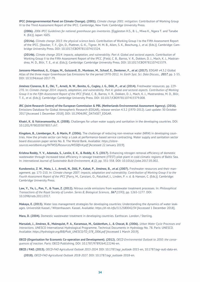
34
IPCC (Intergovernmental Panel on Climate Change). (2001). Climate change 2001: mitigation. Contribution of Working Group III to the Third Assessment Report of the IPCC. Cambridge, New York: Cambridge University Press.
(2006). 2006 IPCC Guidelines for national greenhouse gas inventories. [Eggleston H.S., B. L., Miwa K., Ngara T. and Tanabe K. (Ed.)]. Japan: IGES.
(2014a). Climate change 2013: the physical science basis. Contribution of Working Group I to the Fifth Assessment Report of the IPCC. [Stocker, T. F., Qin, D., Plattner, G.-K., Tignor, M. M. B., Allen, S. K., Boschung, J., et al. (Eds.)]. Cambridge: Cam-bridge University Press. DOI: 10.1017/CBO9781107415324.
(2014b). Climate change 2014: impacts, adaptation, and vulnerability. Part A: Global and sectoral aspects. Contribution of Working Group II to the Fifth Assessment Report of the IPCC. [Field, C. B., Barros, V. R., Dokken, D. J., Mach, K. J., Mastran-drea, M. D., Bilir, T. E., et al. (Eds.)]. Cambridge: Cambridge University Press. DOI: 10.1017/CBO9781107415379.
Janssens-Maenhout, G., Crippa, M., Guizzardi, D., Muntean, M., Schaaf, E., Dentener, F., et al. (2017). EDGAR v4.3.2 Global Atlas of the three major Greenhouse Gas Emissions for the period 1970-2012. In: Earth Syst. Sci. Data Discuss., 2017, pp. 1-55. DOI: 10.5194/essd-2017-79.
Jiménez Cisneros, B. E., Oki, T., Arnell, N. W., Benito, G., Cogley, J. G., Döll, P., et al. (2014). Freshwater resources. pp. 229-270. In: Climate change 2014: impacts, adaptation, and vulnerability. Part A: global and sectoral aspects. Contribution of Working Group II to the Fifth Assessment Report of the IPCC [Field, C. B., Barros, V. R., Dokken, D. J., Mach, K. J., Mastrandrea, M. D., Bilir, T. E., et al. (Eds.)]. Cambridge: Cambridge University Press. DOI: 10.1017/CBO9781107415379.008.
JRC (Joint Research Centre) of the European Commission & PBL (Netherlands Environmental Assessment Agency). (2016). Emissions Database for Global Atmospheric Research (EDGAR), release version 4.3.2 (1970-2012). Last update: 30 October 2017.[Accessed 1 December 2018]. DOI: 10.2904/JRC_DATASET_EDGAR.
Khatri, K. & Vairavamoorthy, K. (2008). Challenges for urban water supply and sanitation in the developing countries. DOI: 10.1201/9780203878057.ch7.
Kingdom, B., Liemberger, R., & Marin, P. (2006). The challenge of reducing non-revenue water (NRW) in developing coun-tries. How the private sector can help: a Look at performance-based service contracting. Water supply and sanitation sector board discussion paper series No. 8. The World Bank. Available: https://sitere-sources.worldbank.org/INTWSS/Resources/WSS8fin4.pdf [Accessed 22 January 2019].
Krishna Reddy, Y. V., Adamala, S., Levlin, E. K., & Reddy, K. S. (2017). Enhancing nitrogen removal efficiency of domestic wastewater through increased total efficiency in sewage treatment (ITEST) pilot plant in cold climatic regions of Baltic Sea. In: International Journal of Sustainable Built Environment, 6 (2), pp. 351-358. DOI: 10.1016/j.ijsbe.2017.05.002.
Kundzewicz, Z. W., Mata, L. J., Arnell, N., Döll, P., Kabat, P., Jiménez, B., et al. (2007). Freshwater resources and their man-agement. pp. 173-210. In: Climate change 2007: impacts, adaptation and vulnerability. Contribution of Working Group II to the Fourth Assessment Report of the IPCC [Parry, M., Canziani, O., Palutikof, J., Linden, P. v. d. & Hanson, C. (Eds.)]. Cambridge: Cambridge University Press.
Law, Y., Ye, L., Pan, Y., & Yuan, Z. (2012). Nitrous oxide emissions from wastewater treatment processes. In: Philosophical Transactions of the Royal Society of London. Series B, Biological Sciences, 367 (1593), pp. 1265-1277. DOI: 10.1098/rstb.2011.0317.
Makaya, E. (2015). Water loss management strategies for developing countries: Understanding the dynamics of water leak-ages. Universität Kassel / Witzenhausen. Kassel. Available: https://d-nb.info/1112580042/34 [Accessed 1 December 2018].
Mara, D. (2004). Domestic wastewater treatment in developing countries. Earthscan. London / Sterling.
Marsalek, J., Jiménez, B., Malmquist, P. A., Karamouz, M., Goldenfum, J., & Chocat, B. (2006). Urban Water Cycle Processes and Interactions. UNESCO International Hydrological Programme, Technical Documents in Hydrology No. 78. Paris: UNESCO. Available: https://hydrologie.org/BIB/Publ_UNESCO/TD_078_2006.pdf [Accessed 1 March 2019].
OECD (Organisation for Economic Co-operation and Development). (2012). OECD Environmental Outlook to 2050: the conse-quences of inaction. Paris: OECD Publishing. DOI: 10.1787/9789264122246-en.
OECD / FAO. (2015). OECD-FAO Agricultural Outlook 2015-2024. DOI: 10.1787/agr_outlook-2015-en, 10.1787/agr-outl-data-en.
(2018). OECD-FAO Agricultural Outlook 2018-2027. DOI: 10.1787/agr_outlook-2018-en.

35
Roser, M. & Ortiz-Ospina, E. (2018). World Population Growth. Oxford Martin Programme on Global Development, University of Oxford. Last update: April 2017. Available: https://ourworldindata.org/world-population-growth [Accessed 20 November 2018].
Timmer, C. P., Falcon, W. P., & Pearson, S. R. (1983). Food policy analysis. In: A World Bank publication. Baltimore, Md. [u.a.]: Johns Hopkins Univ. Press.
UN (United Nations). (2013). Water security and the global water agenda. A UN-Water analytical brief. [Bigas, H. (Ed.)]. Hamil-ton: United Nations University. 37 pages. Available: http://www.unwater.org/downloads/watersecurity_analyticalbrief.pdf [Ac-cessed 02 March 2016].
UNDESA (United Nations Department of Economic and Social Affairs). (2017a). World Population Prospects 2017. Available: https://population.un.org/wpp/ [Accessed 25 December 2018].
(2017b). World Population Prospects: the 2017 revision, methodology of the United Nations population estimates and projections. UN. New York. Available: https://population.un.org/wpp/Publications/Files/WPP2017_Methodology.pdf [Accessed 1 March 2019].
(2018). World Urbanisation Prospects 2018. Available: https://population.un.org/wup/ [Accessed 25 December 2018].
UNSD (United Nations Statistics Division). (2016). Environment Statistics (ENVSTAT). Available: https://un-stats.un.org/unsd/envstats [Accessed 1 March 2019]
Vörösmarty, C. J., McIntyre, P. B., Gessner, M. O., Dudgeon, D., Prusevich, A., Green, P., et al. (2010). Global threats to human water security and river biodiversity. In: Nature, 467 (7315), pp. 555-561. DOI: 10.1038/nature09440.
WaCCliM (Water and Wastewater Companies for Climate Migitation). (2019). ECAM 2.2 Methodology. Available: http://wacclim.org/library/ecam-methodology-guide/ [Accessed 20 March 2019].
WHO (World Health Organisation) & UNICEF (United Nations International Children's Emergency Fund). (2017a). Progress on Drinking water, Sanitation and Hygiene – 2017 update and SDG baselines. Available: https://washdata.org/report/jmp-2017-report-final [Accessed 1 February 2019].
(2017b). The WHO/UNICEF Joint Monitoring Programme for Water Supply, Sanitation and Hygiene (JMP) database. Avail-able: https://washdata.org/ [Accessed 1 February 2019].
(2018). JMP Methodology: 2017 update & SDG baselines. Available: https://washdata.org/report/jmp-methodology-2017-update [Accessed 1 February 2019].
WWAP (World Water Assessment Programme of UN). (2014). The United Nations World Water Development Report 2014: Water and energy. UNESCO. Paris.
(2015). The United Nations World Water Development Report 2015: Water for a sustainable world. UNESCO. Paris.

36
Annex A Overview of all GHG emissions from water and wastewater services
Water abstraction
Water treatment
Water distribution
WW collection
WW treatment
WW discharge
Scope 1 – Direct emissions
CO2, CH4 and N2O emissions from on-site engine stationary fossil fuel combustion
o o o o o o
CH4 from sewers or biological wastewater treatment
o ▪
N2O from sewers or biological wastewater treatment o ▪
Scope 2 – Indirect emissions
Indirect emissions from electric energy
▪ ▪ ▪ ▪ ▪ ▪
Scope 3 – Other indirect emissions
CO2, CH4 and N2O emissions from truck transport of water (drinking water, wastewater, reused water) fossil fuel combustion
o o o
Emissions from the manufacturing of chemical used o o
Emissions from the construction materials used o o o o o o
CH4 and N2O emissions from wastewater discharge without treatment
▪
CO2, CH4 and N2O emissions from sludge transport offsite o
N2O emissions from effluent discharge in receiving waters ▪
o Emissions not quantified, even though they exist ▪ Emissions quantified in the guideline Unless wastewater collection/discharge is by gravity Unless water distribution is gravity (natural) fed
Source: ECAM Methodology version 2.0, with adaptations.

37
Annex B Analysis of key parameters shaping baseline GHG emissions in the urban water cycle
The GHG quantification methodology defined in the IPCC Guideline [2006] provides the basis for the studies on the parame-ters that are critical in shaping baseline scenarios. The measurement follows the general rule that emissions are the product of the magnitude of human activity resulting in emissions taking place in a given period and the average emission rate of a given GHG for a given source relative to units of activity:
𝐸𝑚𝑖𝑠𝑠𝑖𝑜𝑛𝑠 = 𝐴𝑐𝑡𝑖𝑣𝑖𝑡𝑦 𝐷𝑎𝑡𝑎 ∙ 𝐸𝑚𝑖𝑠𝑠𝑖𝑜𝑛 𝐹𝑎𝑐𝑡𝑜𝑟 (𝐴)
Since the activity data and emission factors vary for gases, a concise analysis is detailed hereafter to identify the key param-eters and terms affecting baseline projections of GHG emissions in the urban water cycle.
Key parameters determining CO2 emissions
CO2 emissions as defined by this methodology are those from fossil fuel combustion attributed to purchased electricity. The emissions are quantified as the product of electric power consumption in kilowatt-hours (kWh) and the emission factor in kg CO2 per kWh electricity:
𝐸𝑚𝑖𝑠𝑠𝑖𝑜𝑛𝑠𝐶𝑂2= 𝐴𝑚𝑜𝑢𝑛𝑡 𝑜𝑓 𝐸𝑙𝑒𝑐𝑡𝑟𝑖𝑐𝑖𝑡𝑦 𝐶𝑜𝑛𝑠𝑢𝑚𝑒𝑑 ∙ 𝐸𝑚𝑖𝑠𝑠𝑖𝑜𝑛 𝐹𝑎𝑐𝑡𝑜𝑟 𝑝𝑒𝑟 𝑈𝑛𝑖𝑡 𝐸𝑙𝑒𝑐𝑡𝑟𝑖𝑐𝑖𝑡𝑦 (𝐵)
For the emission factor of grid electricity (EFgrid), the average annual country default value for electricity supply is usually applied, if local data are not available. EFgrid differs from year to year due to reasons such as changes in the fuel mix and effi-ciency improvement of grid power generation. Fuel mix variations can be caused by the gradual structural transformation over a longer term as well as temporary fluctuations in the fuel supply, especially in those countries that are heavily depend-ent on energy import. Consequently, the development trend of the emission factor in the future shall be studied in order to project relevant CO2 emissions.
The evolution of the quantity of electricity consumption is dependent on multiple issues and can be further broken down into subcomponents as follows:
Water supply: • The total population in the service area of water utilities (POPws_resi) • The ratio of residents served by the water utilities (Rws_serv_resi) • The quantity of water to be produced for each resident on average to meet the consumption needs (VOLws/POPws_serv) • The amount of energy required to abstract, treat and distribute each unit volume of water (Ews/VOLws)
Wastewater management: • The total population in the service area of WWTPs (POPww_resi) • The ratio of residents connected to sewers (Rww_conn_resi) and served by WWTPs (Rww_serv_resi) • The average quantity of wastewater to be managed for each resident (VOLww/POPww_serv) • The amount of energy required to collect, treat, and discharge each unit volume of wastewater (Eww/VOLww)
For the detailed evaluation at the sub-stage level, the CO2 emissions from electricity can be expressed in a mathematic rela-tion to the terms described above as:
𝐸𝑚𝑖𝑠𝑠𝑖𝑜𝑛𝑠𝐶𝑂2= ∑ 𝑃𝑂𝑃𝑟𝑒𝑠𝑖 ∙
𝑃𝑂𝑃𝑖
𝑃𝑂𝑃𝑟𝑒𝑠𝑖 ∙
𝑉𝑂𝐿𝑖
𝑃𝑂𝑃𝑖 ∙
𝐸𝑖
𝑉𝑂𝐿𝑖𝑖
∙ 𝐶𝑖
𝐸𝑖
(𝐶)
Where • i refers to the sub-stages in the water and wastewater services. • POPresi refers to the total residents in the service area. • POPi is the population of the resident group that is relevant for stage i concerning access to the water and wastewater
services. In the water supply, POPi is the same for all the sub-stages as those served by water services. In the wastewater management, POPi considered in both collection and discharge is the group connected to sewers, while POPi in treat-ment refers to the population whose wastewater is treated in WWTPs.
• Ci/Ei refers to the carbon intensity of electricity consumed in sub-stage i.

38
Key parameters determining CH4 emissions
CH4 emissions considered in the urban water sector all belong to the wastewater section. The emission process is substan-tially determined by the total organically degradable carbon in wastewater (TOW) and the type of treatment technologies and conditions that characterise the CH4 emission rate from the organics.
The TOW is most important as it indicates the amount of carbon that can be released as CH4. For domestic wastewater, the Biochemical Oxygen Demand over five days, denoted as BOD5, is the most frequently used parameter to measure the organic component. The activity data TOW is thus quantified as a function of the population, their average BOD5 generation per per-son per day, and the length of the period considered:
𝑇𝑂𝑊 = 𝑃𝑂𝑃 ∙ 𝐵𝑂𝐷5 ∙ 𝐷𝑎𝑦𝑠 (𝐷)
The emission factor, expressed in kg CH4 per kg BOD5, is dependent on the treatment and discharge pathway. It is the prod-uct of the maximum CH4 producing potential, usually as default or country-specific value, and the methane correction factor. The latter, which indicates the degree of the anaerobic condition is given as a default value for different technologies and discharge environment by the IPCC.
Since wastewater treatment removes a large fraction of BOD with sludge, the fraction of TOW that remains in the wastewater as the potential source of CH4 emissions can be greatly reduced. Although the anaerobic digestion of the sludge also converts the removed organics into methane which is partly released as biogas, the emission in this step can be con-trolled to zero through the valorisation of biogas to an energy source.
Consequently, the development of CH4 emissions in baseline scenarios, i.e., in the existing treatment system and discharge environment, is predominantly determined by variations of organics generated by the total population and the degree of wastewater treatment including methane recovery. Therefore, three questions arise in the evaluation of BAU scenarios, namely:
• The number of the total population in the service area of WWTPs (POPww_resi) • The ratio of residents connected to sewers (Rww_conn_resi) and served by WWTPs (Rww_serv_resi) • The quantity of BOD5 generated by each resident per day in the same length of the assessment period (BOD5)
Thus, the relation between CH4 emissions and the parameters can be expressed as:
𝐸𝑚𝑖𝑠𝑠𝑖𝑜𝑛𝑠𝐶𝐻4= [∑(𝑃𝑂𝑃𝑟𝑒𝑠𝑖 ∙ 𝑅𝑗) ∙ (1 − 𝑆𝑗
𝐵𝑂𝐷) ∙ 𝑇𝑗𝐶𝐻4
𝑗
] ∙ 𝐵𝑂𝐷5𝑎.𝑝. (𝐸)
Where • j indicates the resident groups with different connection degrees, divided into those whose wastewater is not collected,
collected but not treated, and fully collected and treated. • POPresi refers to the total residents in the service area. • Rj is the proportion of group j in the total population POPresi . • 𝑆𝑗
𝐵𝑂𝐷 is the ratio of BOD removal in treatment processes of group j. For those whose wastewater is not treated, the result equals zero.
• Tj refers to the emission rate associated with the treatment/discharge system of group j. • 𝐵𝑂𝐷5
𝑎.𝑝. refers to the per person BOD5 generation in the assessment period.
Key parameters determining N2O emissions
In order to quantify N2O emissions in the urban water cycle, the activity data required are the total nitrogen (TN) load in the sewage, which can be calculated as the product of the population producing this part of wastewater, their average protein consumption quantity per person per year, the length of the period considered and the nitrogen content in per unit protein. The result is corrected by default parameters as defined by the IPCC [2006] to include non-consumed protein washed away as food waste and protein contained in co-discharged industrial or commercial wastewater. Thus, the nitrogen content is estimated as:
𝑇𝑁 = 𝑃𝑂𝑃 ∙ (𝑃𝑅𝑂𝑇𝐸𝐼𝑁
365 ∙ 𝐷𝑎𝑦𝑠) ∙ 𝐹𝑁𝑖𝑡𝑟𝑜𝑔𝑒𝑛 𝑖𝑛 𝑃𝑟𝑜𝑡𝑒𝑖𝑛 ∙ 𝐹𝑁𝑂𝑁−𝐶𝑂𝑁 ∙ 𝐹𝐼𝑁𝐷−𝐶𝑂𝑀 (𝐹)

39
At the same time, the N2O emission factor associated with receiving water for untreated wastewater and discharged efflu-ents from WWTPs is a fixed value defined by the IPCC [2006] based on assumptions regarding the occurrence of nitrification and denitrification in rivers and estuaries.
The nitrogen compounds in sewage can be removed by different technologies during wastewater treatment. This reduces the nitrogen content in the treated effluents as well as the potential quantity of N2O emissions in the natural water body. The ECAM tool also considers emissions during the treatment, but this component of the emissions is estimated at only 3.2 g N2O per person per year [IPCC, 2006]. Thus, the total N2O emissions of treated sewage are significantly lower than the situation, providing the wastewater is directly discharged without treatment.
In summary, baseline N2O emissions in an existing technical system are predominantly determined by variations of the pro-tein generation as well as the coverage and degree of wastewater treatment. For future studies on BAU scenarios, three sep-arate issues are of importance:
• The total population in the service area of WWTPs (POPww_resi) • The ratio of residents connected to sewers (Rww_conn_resi) and served by WWTPs (Rww_serv_resi) • The quantity of protein consumption per person per day in the same length of the assessment period (PROTEIN)
Equation (G) shows the mathematical connection between the parameters and N2O emissions:
𝐸𝑚𝑖𝑠𝑠𝑖𝑜𝑛𝑠𝑁2𝑂 = [∑(𝑃𝑂𝑃𝑟𝑒𝑠𝑖 ∙ 𝑅𝑗) ∙ (1 − 𝑆𝑗𝑁) × 𝑇𝑗
𝑁2𝑂
𝑗
] × 𝑃𝑅𝑂𝑇𝐸𝐼𝑁𝑎.𝑝. (𝐺)
Where • j indicates the resident groups with different connection degrees, divided into those whose wastewater is not collected,
collected but not treated, and fully collected and treated. • POPresi refers to the total residents in the service area. • Rj is the proportion of group j in the total population POPresi . • 𝑆𝑗
𝑁 is the ratio of nitrogen removal of group j. For those whose wastewater is not treated, the result equals zero. • Tj refers to the emission rate associated with the treatment/discharge system of group j. • PROTEINa.p. is the per person protein consumption in the assessment period.
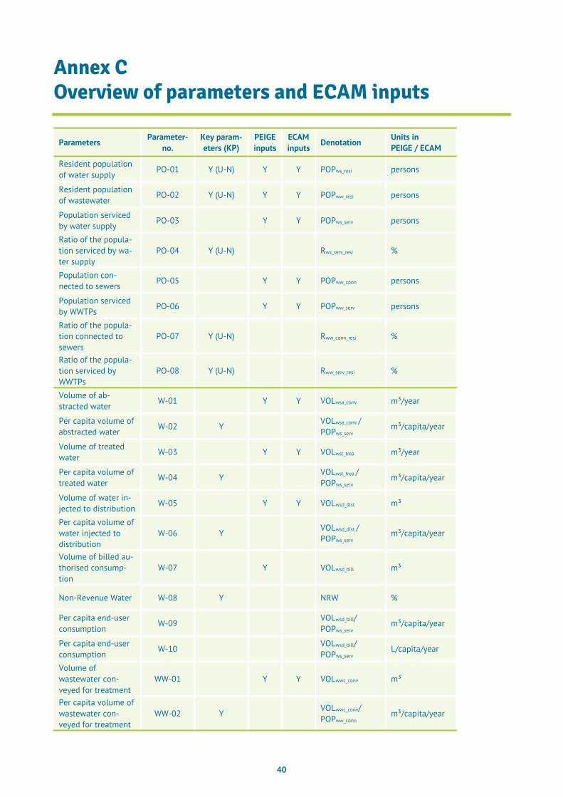
40
Annex C Overview of parameters and ECAM inputs
Parameters Parameter-no.
Key param-eters (KP)
PEIGE inputs
ECAM inputs Denotation Units in
PEIGE / ECAM
Resident population of water supply PO-01 Y (U-N) Y Y POPws_resi persons
Resident population of wastewater PO-02 Y (U-N) Y Y POPww_resi persons
Population serviced by water supply PO-03 Y Y POPws_serv persons
Ratio of the popula-tion serviced by wa-ter supply
PO-04 Y (U-N) Rws_serv_resi %
Population con-nected to sewers PO-05 Y Y POPww_conn persons
Population serviced by WWTPs PO-06 Y Y POPww_serv persons
Ratio of the popula-tion connected to sewers
PO-07 Y (U-N) Rww_conn_resi %
Ratio of the popula-tion serviced by WWTPs
PO-08 Y (U-N) Rww_serv_resi %
Volume of ab-stracted water W-01 Y Y VOLwsa_conv m³/year
Per capita volume of abstracted water W-02 Y VOLwsa_conv /
POPws_serv m³/capita/year
Volume of treated water W-03 Y Y VOLwst_trea m³/year
Per capita volume of treated water W-04 Y VOLwst_trea /
POPws_serv m³/capita/year
Volume of water in-jected to distribution W-05 Y Y VOLwsd_dist m³
Per capita volume of water injected to distribution
W-06 Y VOLwsd_dist / POPws_serv
m³/capita/year
Volume of billed au-thorised consump-tion
W-07 Y VOLwsd_bill m³
Non-Revenue Water W-08 Y NRW %
Per capita end-user consumption
W-09 VOLwsd_bill/ POPws_serv
m³/capita/year
Per capita end-user consumption W-10 VOLwsd_bill/
POPws_serv L/capita/year
Volume of wastewater con-veyed for treatment
WW-01 Y Y VOLwwc_conv m³
Per capita volume of wastewater con-veyed for treatment
WW-02 Y VOLwwc_conv/ POPww_conn
m³/capita/year

41
Parameters Parameter-no.
Key param-eters (KP)
PEIGE inputs
ECAM inputs Denotation Units in
PEIGE / ECAM
Volume of treated wastewater WW-03 Y Y VOLwwt_trea m³
Per capita volume of treated wastewater
WW-04 Y VOLwwt_trea/POPw
w_serv m³/capita/year
Volume of discharged effluent to water body
WW-05 Y Y VOLwwd_disc m³
Per capita volume of discharged effluent WW-06 Y VOLwwd_disc/POPw
w_conn m³/capita/year
Volume of reused effluent
WW-07 Y Y VOLwwd_nonp m³
Per capita volume of reused effluent WW-08 Y VOLwwd_nonp/POP
ww_conn m³/capita/year
Volume of discharged & reused effluent
WW-09 VOLwwd= VOLwwd_disc+VOLw
wd_nonp m³
Per capita volume of discharged & reused effluent
WW-10 VOLwwd/ POPww_conn
m³/capita/year
Influent BOD5 load WW-11 Y Y BODinfl kg
Effluent BOD5 load WW-12 Y Y BODeffl kg
BOD removed as sludge WW-13 Y Y BODslud kg
Total nitrogen concentration in the effluent
WW-14 Y Y NCeffl mg/L
Ratio of removed nitrogen in treated wastewater
WW-15 RN_wwt_rmvd %
Electricity consumed for total water supply
E-01 Y (A) Y (A) Ews kWh
Energy intensity of total water supply
E-02 Y (A) Ews/ VOLwsd_dist kWh/m³
Electricity consumed for water abstraction
E-03 Y Y Ewsa kWh
Energy intensity of water abstraction
E-04 Y Ewsa/ VOLwsa_conv kWh/m³
Electricity consumed for water treatment
E-05 Y Y Ewst kWh
Energy intensity of water treatment
E-06 Y Ewst/ VOLwst_trea kWh/m³
Electricity consumed for water distribution
E-07 Y Y Ewsd kWh
Energy intensity of water distribution E-08 Y Ewsd/ VOLwsd_dist kWh/m³
Electricity consumed for total wastewater E-09 Y (A) Y (A) Eww kWh
Energy intensity of total wastewater E-10 Y (A) Eww/ VOLwwt_trea kWh/m³
Electricity consumed for wastewater col-lection
E-11 Y Y Ewwc kWh
Energy intensity of wastewater collec-tion
E-12 Y Ewwc/ VOLwwc_conv kWh/m³
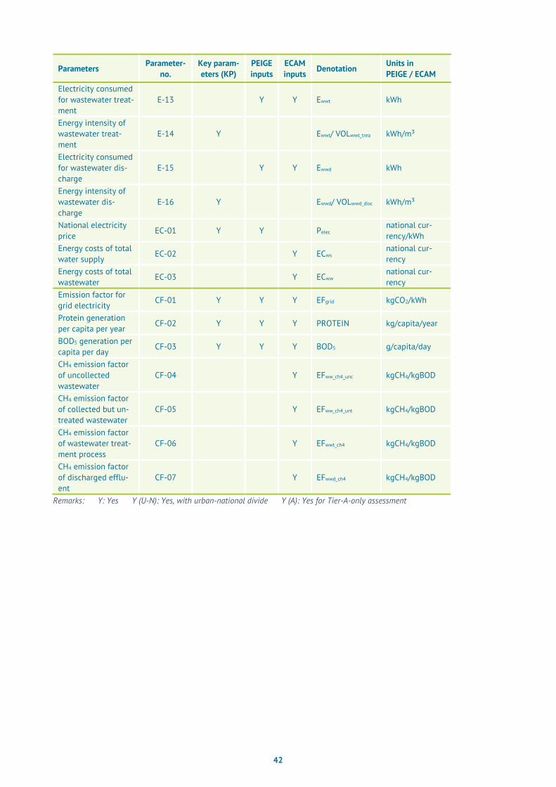
42
Parameters Parameter-no.
Key param-eters (KP)
PEIGE inputs
ECAM inputs Denotation Units in
PEIGE / ECAM
Electricity consumed for wastewater treat-ment
E-13 Y Y Ewwt kWh
Energy intensity of wastewater treat-ment
E-14 Y Ewwt/ VOLwwt_trea kWh/m³
Electricity consumed for wastewater dis-charge
E-15 Y Y Ewwd kWh
Energy intensity of wastewater dis-charge
E-16 Y Ewwd/ VOLwwd_disc kWh/m³
National electricity price EC-01 Y Y Pelec
national cur-rency/kWh
Energy costs of total water supply EC-02 Y ECws
national cur-rency
Energy costs of total wastewater EC-03 Y ECww national cur-
rency Emission factor for grid electricity CF-01 Y Y Y EFgrid kgCO2/kWh
Protein generation per capita per year CF-02 Y Y Y PROTEIN kg/capita/year
BOD5 generation per capita per day CF-03 Y Y Y BOD5 g/capita/day
CH4 emission factor of uncollected wastewater
CF-04 Y EFww_ch4_unc kgCH4/kgBOD
CH4 emission factor of collected but un-treated wastewater
CF-05 Y EFww_ch4_unt kgCH4/kgBOD
CH4 emission factor of wastewater treat-ment process
CF-06 Y EFwwt_ch4 kgCH4/kgBOD
CH4 emission factor of discharged efflu-ent
CF-07 Y EFwwd_ch4 kgCH4/kgBOD
Remarks: Y: Yes Y (U-N): Yes, with urban-national divide Y (A): Yes for Tier-A-only assessment
43
Annex D Projection of nitrogen concentration in the effluent
The nitrogen content in the effluent is the result of the TN of all collected wastewater minus the part that is removed in the treatment. The corresponding nitrogen content NCeffl can be expressed as:
𝑁𝐶𝑒𝑓𝑓𝑙 =𝑇𝑁𝑐𝑜𝑙𝑙𝑒𝑐𝑡𝑒𝑑 𝑊𝑊 − 𝑇𝑁𝑡𝑟𝑒𝑎𝑡𝑒𝑑 𝑊𝑊 ∙ 𝑅𝑁_𝑤𝑤𝑡_𝑟𝑚𝑣𝑑
𝑉𝑂𝐿𝑤𝑤𝑐
(𝐻)
Where RN_wwt_rmvd refers to the ratio of nitrogen removed from the treated wastewater.
Based on equation (F) in Annex B and assuming that the technical performance remains stable in the BAU scenarios, equa-tion (H) can be applied to project nitrogen concentration in year t (𝑁𝐶𝑒𝑓𝑓𝑙
𝑡 ) and extended as:
𝑁𝐶𝑒𝑓𝑓𝑙𝑡 [𝑚𝑔/𝐿] =
[𝑃𝑂𝑃𝑤𝑤_𝑐𝑜𝑛𝑛𝑡 − 𝑃𝑂𝑃𝑤𝑤_𝑠𝑒𝑟𝑣
𝑡 ∙ 𝑅𝑁_𝑤𝑤𝑡_𝑟𝑚𝑣𝑑] ∙ 𝑃𝑅𝑂𝑇𝐸𝐼𝑁𝑡 ∙ 0.16 ∙ 1.1 ∙ 1.25
𝑉𝑂𝐿𝑤𝑤𝑐𝑡
∙ 1000 (𝐼)
Where
• 1000: NCeffl is converted from kg/m³ to mg/L • PROTEIN: per capita per year protein consumption in kg protein • 0.16: factor of nitrogen content in per unit protein Fnitrogen in protein, default = 0.16 kg N/kg protein • 1.1: factor of non-consumed protein as food waste FNON-CON, 1.1 for developing countries • 1.25: factor for industrial/commercial co-discharged protein into the sewage system FIND-COM
While all other parameters are projected with the approches developed in various parts of Chapter 0, the value of the term RN_wwt_rmvd needs to be determined.
On the national level, the average value of RN_wwt_rmvd is suggested in Chapter 2.3.12 based on the distribution of different treatment technologies. The associated national mean of NCeffl as PEIGE inputs is also provided in this chapter.
On the utility level, the value of RN_wwt_rmvd can be identified methmatically through on-site data. Since RN_wwt_rmvd is assumed to be fixed over the entire period of BAU scenarios, equation (I) can be re-formulated as a function of RN_wwt_rmvd depending on other variables in year t as:
𝑅𝑁_𝑤𝑤𝑡_𝑟𝑚𝑣𝑑 =𝑃𝑂𝑃𝑤𝑤_𝑐𝑜𝑛𝑛
𝑡
𝑃𝑂𝑃𝑤𝑤_𝑠𝑒𝑟𝑣𝑡
−
(𝑉𝑂𝐿𝑤𝑤𝑐𝑡 ∙
𝑁𝐶𝑒𝑓𝑓𝑙𝑡
1000)
𝑃𝑂𝑃𝑤𝑤_𝑠𝑒𝑟𝑣𝑡 ∙ 𝑃𝑅𝑂𝑇𝐸𝐼𝑁𝑡 ∙ 0.16 ∙ 1.1 ∙ 1.25
(𝐽)
Based on equation (J), the current (fixed) value of RN_wwt_rmvd can be determined mathematically using PEIGE inputs (2015 val-ues) of the items POPww_conn, POPww_serv, PROTEIN, VOLwwd and NCeffl:
𝑅𝑁_𝑤𝑤𝑡_𝑟𝑚𝑣𝑑 =𝑃𝑂𝑃𝑤𝑤_𝑐𝑜𝑛𝑛
2015
𝑃𝑂𝑃𝑤𝑤_𝑠𝑒𝑟𝑣2015
−
(𝑉𝑂𝐿𝑤𝑤𝑐2015 ∙
𝑁𝐶𝑒𝑓𝑓𝑙2015
1000)
𝑃𝑂𝑃𝑤𝑤_𝑠𝑒𝑟𝑣2015 ∙ 𝑃𝑅𝑂𝑇𝐸𝐼𝑁2015 ∙ 0.16 ∙ 1.1 ∙ 1.25
(𝐾)
Both equation (I) and (K) have been programmed in PEIGE, which calculates RN_wwt_rmvd and NCeffl in BAU scenarios in mg/L automatically after users enter the current NCeffl – of a single utility or the average national value – into the Excel tool.

44
Annex E Statistical methods for calculating average growth rates
Average growth rates are widely used in scientific research as well as in daily life. They describe the course of changes of a certain variable during a certain period. Growth rates are subject to assumptions about patterns of growth. In this guideline, three different types of annual growth rates are applied, namely arithmetic, exponential, and geometrical growth. In this section, all three patterns will be described briefly according to UNSD [UNESCAP, 2015].
Arithmetic growth rates
Arithmetic growth means the variable decreases or increases by a constant absolute quantity in each period unit and implies a linear trend. The average arithmetic growth rate (rAG) of the variable X between the time point 0 and t is derived as:
𝑟𝐴𝐺 =(
𝑋𝑡
𝑋0− 1)
𝑡(𝐿)
Consequently, the value of the variable X at the time point t is calculated in relation to the value at the starting time point 0 as:
𝑋𝑡 = 𝑋0 ∙ (1 + 𝑟𝐴𝐺 ∙ 𝑡) (𝑀)
Xt can also be quantified based on the value at the previous time point t-1 through:
𝑋𝑡 = 𝑋𝑡−1 + (𝑟𝐴𝐺 ∙ 𝑋0) (𝑁)
For the BAU scenario establishment, the infrastructure coverage and NRW are assumed to undergo an arithmetic trend.
Exponential growth rates
Exponential growth means the growth compounds continuously at every instant of time, or the variable grows at a constant rate at every infinitesimal of time. It is the limiting case of compounding. The exponential growth rate is mostly used in the scientific field of biology. For the BAU scenarios, the population is assumed to grow exponentially as it is a conventional method adopted by international organisations such as the UN.
The average exponential growth rate (rEG) between time point t and 0 is calculated by:
𝑟𝐸𝐺 =𝐿𝑁 (
𝑋𝑡
𝑋0)
𝑡(𝑂)
Consequently, the value of the variable X at the time point t is calculated in relation to the value at the starting time point 0 as:
𝑋𝑡 = 𝑋0 ∙ 𝑒(𝑟𝐸𝐺∙𝑡) (𝑃)
In the BAU Guideline, the absolute quantity of population has been projected by UNDESA for every single year in the future. Thus, the corresponding growth rate varies from year to year, denoted as rt and derived from UN data through:
𝑟𝑡 = 𝐿𝑁 (𝑃𝑂𝑃𝑡
𝑃𝑂𝑃𝑡−1) (𝑄)
Thus, PEIGE calculates the population of year t based on the population of the year before and the embedded growth rate rt
as:
𝑃𝑂𝑃𝑡 = 𝑃𝑂𝑃𝑡−1 ∙ 𝑒𝑟𝑡 (𝑅)

45
Hence, the population of year t is related to the population of the starting year POP0 as follows:
𝑃𝑂𝑃𝑡 = 𝑃𝑂𝑃0 ∙ 𝑒𝑟1 ∙ 𝑒𝑟2 … ∙ 𝑒𝑟𝑡 = 𝑃𝑂𝑃0 ∙ 𝑒(𝑟1+𝑟2…+𝑟𝑡) (𝑆)
Geometric growth rates
Geometric growth is a special case of exponential change. It occurs when the variable decreases or increases by a certain ratio from one period to the other. Since the variable is increasing, geometric growth implies incremental changes are be-coming larger in the absolute quantity. The geometric growth method is one of the prevailing patterns used in practice. This guideline applies it to project all variables except the two described above.
Geometric average growth rate, also widely named compound annual growth rate (CAGR), is calculated as follows:
𝑟𝐶𝐴𝐺𝑅 = (𝑋𝑡
𝑋0)
1𝑡
− 1 (𝑇)
Consequently, the value of the variable X at the time point t is calculated in relation to the value at the time point 0 as:
𝑋𝑡 = 𝑋0 ∙ (1 + 𝑟𝐶𝐴𝑅𝐺)𝑡 (𝑈)
The relation of the value at the time point t with the value at the previous time point t-1 is measured as:
𝑋𝑡 = 𝑋𝑡−1 ∙ 𝑟𝐶𝐴𝐺𝑅 (𝑉)
All three patterns do not take into consideration the intermediate values between the first and last points. Therefore, the calculated growth rates are very sensitive to the choice of starting and ending positions and very reactive to temporary fluc-tuations. Hence, in the case of higher data uncertainty, the average value over three consecutive years is used for the start and end values in the BAU methodology, which is also a common practice.
For more detailed information, please refer to UNESCAP [2015].

46
www.wacclim.org
Published by: c/o Deutsche Gesellschaft für Internationale Zusammenarbeit (GIZ) GmbH Postfach 5180 / 65726 Eschborn / Germany T: +49 61 96 79-0 E: [email protected] I: www.giz.de
This project is part of the International Climate Initiative (IKI): www.international-climate-initiative.com/en
c/o IWA – International Water Association Alliance House / 12 Caxton Street / London SW1H 0QS / United Kingdom T: +44 207 654 5500 E: [email protected] I: www.iwa-network.org
Contact: [email protected] www.wacclim.org @WaCCliM_Projekt October 2020


