НАУЧНИ ТРУДОВЕ НА РУСЕНСКИЯ УНИВЕРСИТЕТ – 2014, том 53, серия 1.2

- 194 -

Methodology for Numerical Modeling the Performance

of Vertical Axis Wind Turbines

Ahmed Ahmedov Krasimir Tujarov Gencho Popov

Methodology for Numerical Modeling the Performance of Vertical Axis Wind Turbines: This

paper presents a methodology for developing a numerical simulation procedure regarding vertical axis wind

turbines Savonius type. Therefore the mains steps of developing the CFD analysis have been introduced –

creating a geometrical model, generating a computational mesh, solver setup and carrying out the modeling.

Key words: ANSYS Fluent, VAWT, Numerical Modelling, y+

Criteria, Turbulence Model.

INTRODUCTION

The aerodynamics of the Vertical Axis Wind Turbines (VAWT) is characterized by its

pronounced unsteadiness, mainly due to the constantly changing angular position of their

blades during the machine operation. This is the main reason for the constant changes in

the values of the relative velocity of the air flow acting on the rotor blades and the

Reynolds number. The complex unsteady flow through the rotor of a VAWT at the majority

of the cases is impossible to be investigated with the classical aerodynamic models like

the streamtube and the vortex models [1, 2]. This problem can be avoided by using a

numerical modeling approach – Computational Fluid Dynamics (CFD). The CFD modeling

allows the precise modeling of the flow (vortex structures, three-dimensional effect, strut

influence etc.). The conduction of a CFD modeling provides data about the flow such as,

velocity fields, pressure, temperature etc. Also it allows us to visualize these results by

using multicolor fields, isolines/surfaces, visualizing the flow trajectories by uncontentious

lines or vector fields. The results acquired from a CFD modeling can be compared to those

obtained by experimental study in an aerodynamic channel, thus leading to significant

reduction in the expenses for experimental investigations. CFD modeling is considerably

computational expensive approach. Even when investigating a relatively simple problem

the hardware and computational time demands are high. Furthermore the accuracy of the

results is hard to be evaluated in the absence or scarce of experimental data related to the

studied problems.

Aim and Tasks

The aim of the present paper is the development of a methodology for numerical

modeling the operation of a Savonius VAWT with two semicircular blades by the physical

models included in the CFD software ANSYS Fluent 14.0.

For achieving of the aim the following tasks have been solved: an adequate two

dimensional model simulating the operation of a rotating turbine have been developed; a

simulation of the flow passing through the rotor is carried out; the performance

characteristics of the turbine have been obtained.

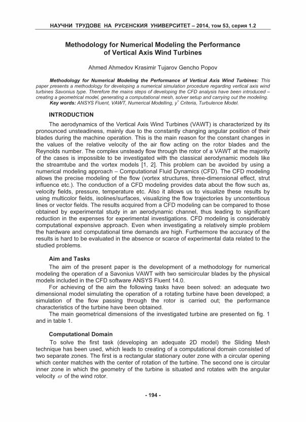
The main geometrical dimensions of the investigated turbine are presented on fig. 1

and in table 1.

Computational Domain

To solve the first task (developing an adequate 2D model) the Sliding Mesh

technique has been used, which leads to creating of a computational domain consisted of

two separate zones. The first is a rectangular stationary outer zone with a circular opening

which center matches with the center of rotation of the turbine. The second one is circular

inner zone in which the geometry of the turbine is situated and rotates with the angular

velocity ω of the wind rotor.

НАУЧНИ ТРУДОВЕ НА РУСЕНСКИЯ УНИВЕРСИТЕТ – 2014, том 53, серия 1.2

- 195 -

Fig. 1 Scheme of the Savonius rotor

Table 1

Main geometrical parameters of the investigated turbine

Diameter D, m 0.1

Rotor High H, m 0,1

Eccentricity е, m 0.35

Number of Blades N 2

Blade Thickness b, m 0,001

End Plate Diameter DEP

, m 0.03

Blade Diameter d, m 0.06

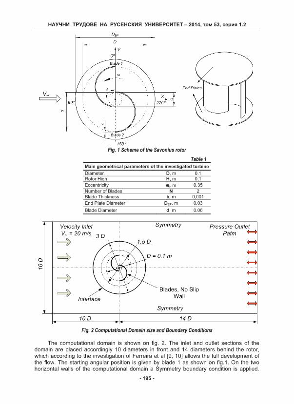
Fig. 2 Computational Domain size and Boundary Conditions

The computational domain is shown on fig. 2. The inlet and outlet sections of the

domain are placed accordingly 10 diameters in front and 14 diameters behind the rotor,

which according to the investigation of Ferreira et al [9, 10] allows the full development of

the flow. The starting angular position is given by blade 1 as shown on fig.1. On the two

horizontal walls of the computational domain a Symmetry boundary condition is applied.

НАУЧНИ ТРУДОВЕ НА РУСЕНСКИЯ УНИВЕРСИТЕТ – 2014, том 53, серия 1.2

- 196 -

On the circular wall an Interface boundary condition is applied, which provides the

continuity of the flow from the outer to the inner computational zone.

Inner computational zone

The diameter of the inner computational zone is three times bigger than the rotor

diameter, fig. 3. This provides enough space around him for adequate modeling of the

computational mesh. Inside the inner computational zone the rotor is surrounded by a

control circle with diameter 1.5D (0.150 m). In contrast with the Interface boundary

condition the boundary of the control circle has no physical influence on the flow its only

purpose is to provide precise control over the computational mesh in the near rotor area.

This control is achieved by applying Sizing Functions which operates in direction from the

blade surface towards the control circle and functions acting from the control circle towards

the whole inner computational domain. The boundary condition Interior is applied over the

surface of the control circle, which provides undisturbed mesh generation on both sides of

the circle.

Computational Mesh Generation

For the both zones of the 2D model an unstructured computational mesh has been

generated. According to an investigation carried out be Cummings [5] this type of mesh

provides consistent accuracy in modeling the rotation of the turbine. Main advantages of

the unstructured mesh are its simple handling and excellent application in describing

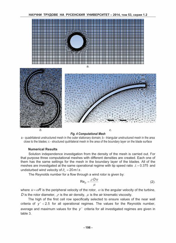
complex geometries. On fig. 3 and 4 the computational mesh used in the present study is

presented. For the outer stationary zone an unstructured quadrilateral mesh has been

used, while for the inner zone an unstructured triangular mesh has been used. Providing a

mesh with the same parameters on both sides of the Interface area leads to faster solution

convergence [4]. The computational cells Growth Factor applied inside the control circle

and as well as outside of it is set to be 1.2. This provides a gradual increase in the

computational cells size in direction away from the rotor. The near blade mesh is

controlled by the use of a Sizing Functions. A total of three Sizing Functions have been

used inside the control circle: the first one is applied over the convex and concave sides of

the blades and it provides cells with length mmx 1=Δ ; the second one is applied over the

blades end edges and it provides cell length mmx 25.0=Δ ; the third function is applied

over the control circle and it allows the generation of cells with length mmx 1=Δ . The

accuracy of the solution highly depends from the proper modeling of the laminar sublayer

over the surface of the blades. In the area of the boundary layer a refined structured

quadrilateral mesh has been used. The sizes of the computational cells used in the

different areas of the computational domain are shown in table 2.

The y

+

criteria have significant effect over the quality of the mesh and the

performance of the turbulence model. This non-dimensional parameter characterizes the

distance from the wall (the blade) to the first layer of cells. The near wall criteria is given

by:

μ

ρτ

yU

y =

+

(1)

where ρ is the air density, y is the normal distance from the wall to the first computational

node from the mesh, ρτωτ

/=U is the frictional velocity, ( )yu ∂∂= /μτω

is the near wall

tangential stress, defined with the near wall velocity gradient in normal direction, μ is the

air dynamic viscosity.

НАУЧНИ ТРУДОВЕ НА РУСЕНСКИЯ УНИВЕРСИТЕТ – 2014, том 53, серия 1.2

- 197 -

Table 2

Stationary Outer Domain

Maximum Size 10 mm

Size at the Interface Area 2.5 mm

Inner Rotational Domain

Maximum Size 2.5 mm

Size in the Near Blade Area 1 mm

Cell Length on Blade Surface 1 mm

First Cell Row High 0.01 mm

Growth Factor 1.2

The precision of the numerical modeling is

determined by the value of the y+

criteria:

• 30030 <<

+

y this range is

recommended for simulations with activated

wall function, in these cases the mesh allows

flow modeling only to the turbulent region

30>

+

y .

• 51 <<

+

y these values are typical for

meshes fine enough to allow modeling of the boundary laminar sublayer.

The linear (laminar sublayer) and logarithmic (turbulence sublayer) near wall laws are

combined in a single one which gives the shape of the velocity profile of the first row of

computational cells no matter the value of the y+

criteria.

Solver Setup

The Navier-Stokes partial differential equations for incompressible fluid flow are

appropriate for modeling the operation of a Savonius VAWT, due to the fact that the flow

velocity in the rotor region do not exceeds 0.3 Mach. The operation of the turbine is

characterized wit high flow unsteadiness due to which the unsteady form of the governing

equations is used. The system of discretized Navier-Stokes momentum equations and the

continuity equation [4] are solved with the segregate scheme SIMPLEC (Semi-Implicit

Method for Pressure-Linked Equations-Corrected).

For determining the share stresses the turbulence model SSTk ω− (Shear Stress

Transition) is used. This model is consisted by two equations and combines the

advantages of the ε−k model for the main flow modeling and the ω−k model for the

good boundary layer modeling [6, 7]. Using this turbulence model Abraham et al. [3]

carried out a two dimensional modeling of a Savonius rotor operation. When comparing

the theoretical and experimental results, they concluded that in the theoretical

characteristic the form of the curve is well reproduced but the values were increased. In

the three dimensional study carried out by Plourde et al. [8] with the SSTk ω− turbulence

model it can be seen a very good agreement between the theoretical and experimental

results.

The value of the chosen time step corresponds to the time for which the turbine

changes its angular position with°

=Δ 1θ . The results from the modelling are saved on

every tenth time step in order to avoid large amounts of data. The number of inner

iterations for each time step is set to 100. This allows the solution to converge when the

residues of the calculated variables reaches values of the order 10-4

. For all simulated

cases the turbulence intensity is set to be 10%. The investigation of the wind turbine is

carried out for 14 different operational regimes.

Fig. 3 Unstructured triangular mesh

in the near rotor area

НАУЧНИ ТРУДОВЕ НА РУСЕНСКИЯ УНИВЕРСИТЕТ – 2014, том 53, серия 1.2

- 198 -

a.

b. c.

Fig. 4 Computational Mesh

a - quadrilateral unstructured mesh in the outer stationary domain; b - triangular unstructured mesh in the area

close to the blades; c - structured qudrilateral mesh in the area of the boundary layer on the blade surface

Numerical Results

Solution independence investigation from the density of the mesh is carried out. For

that purpose three computational meshes with different densities are created. Each one of

them has the same settings for the mesh in the boundary layer of the blades. All of the

meshes are investigated at the same operational regime with tip speed ratio 375.0=λ and

undisturbed wind velocity of sm /20=

∞

ϑ .

The Reynolds number for a flow through a wind rotor is given by:

μ

ρ uD

D=Re (2).

where Ru ω= is the peripheral velocity of the rotor, ω is the angular velocity of the turbine,

D is the rotor diameter, ρ is the air density, μ is the air kinematic viscosity.

The high of the first cell row specifically selected to ensure values of the near wall

criteria of 5.2<

+

y for all operational regimes. The values for the Reynolds number,

average and maximum values for the +

y criteria for all investigated regimes are given in

table 3.

НАУЧНИ ТРУДОВЕ НА РУСЕНСКИЯ УНИВЕРСИТЕТ – 2014, том 53, серия 1.2

- 199 -

The values of the +

y criteria are obtained after

processing the mesh data for blade 1 at four different

angular positions°°°°

= 270,180,90,0θ .

Fig. 5 show the comparison between the torques

generated from the Savonius rotor obtained from three

computational meshes with densities: Mesh 1 – 16750

cells; Mesh 2 – 111550 cells; Mesh 3 182100 cells. The

results are showing that the torque obtained from the

modeling with Mesh 2 is matching with the torque

obtained from Mesh 3. Therefore the solution

independence is achieved with Mesh 2. From here on

Mesh 2 is used for all the simulations.

Also a solution independence study from the

number of rotor revolutions is carried out. Fig. 6 depicts

the torque changes for six full revolutions of the turbine.

The chart is showing that periodicity in the solution is

achieved after the fifth revolution. Therefore all the

simulations are carried out for six full revolutions. All of

the presented data is obtained from the last revolution.

Fig. 5 Solution independence from the mesh

density

Fig. 6 Solution independence from the number of

rotor revolutions

Fig. 7 Rotor torque against the rotational velocity Fig. 8 Rotor output power against rotational

velocity

The results for the average values of the torque against the rotational velocity are

shown on fig. 7. As can be seen from the graphic the maximum torque value is achieved in

Table 3

λ ReD Y

+

AVE Y

+

MAX

0.025 3422 0.74 1.79

0.0625 8557 0.78 1.64

0.125 17114 0.87 1.96

0.25 34229 0.81 1.78

0.375 51344 0.72 2

0.5 68458 0.78 2.3

0.625 85573 0.75 2.2

0.75 102688 0.75 2.2

0.875 119802 0.76 1.74

1 136917 0.73 1.71

1.125 154032 0.73 1.74

1.25 171146 0.81 1.61

1.5 205376 0.78 1.83

2 273834 0.78 1.52

НАУЧНИ ТРУДОВЕ НА РУСЕНСКИЯ УНИВЕРСИТЕТ – 2014, том 53, серия 1.2

- 200 -

the area of the lowest rpm’s. Its maximum value is NmM 7.0≈ reached at1

min240

−

≈n .

With the increase of the rotational velocity the torque is decreasing until it reaches values

around zero at1

min7640

−

≈n . On fig. 8 presents the turbine output power against the

rotational velocity. The output power is obtained by:

ωMP = . (3)

The maximum value of the output power is WP 150≈ achieved at1

min4800

−

≈n .

Conclusions

The presented methodology for numerical, two dimensional modeling the operation of

a VAWT uses the technique Sliding Mesh. The size of the computational domain is

selected according to recommendations from the reference literature.

The values for the y+

criteria at all operational regimes do not exceed 2.5, which

ensure the modeling of the boundary laminar sublayer.

A mesh independence study is carried out, through which the mesh with the optimal

density is evaluated.

From the solution independence study from the number of rotor revolutions is found

that the periodicity in the solution is achieved after the fifth revolution.

Теоретичните резултати ясно показват адекватността на метода да моделира

работата на вятърните турбини с вертикална ос. Предложената методика е и

адекватен инструмент за получаване на теоретичните им характеристики.

The theoretical results clearly show the adequacy of this approach to successfully

model the operation of VAWT. The proposed methodology is also an adequate tool for

obtaining their theoretical characteristics.

Reference

[1] Ахмедов A., Кр. Тужаров, Г. Попов, И. Желева, И. Николаев; Кл. Климентов.

Теоретични модели за изследване на ветротурбини с вертикална ос на въртене

тип Дариус – моментни модели. Механика на машините, 2013, брой 2, стр. 27-

32, ISSN 0861-9727.

[2] Ахмедов А, Кр. Тужаров, Г. Попов, И. Желева, Кл. Климентов, И. Николаев.

Вихров и каскаден модели за изследване на ветротурбини с вертикална ос на

въртене тип Дариус. В: Научни трудове на РУ “А. Кънчев”, том 51, сер. 1.2, Русе

2012, Русе, 2012.

[3] Abraham J P, Mowry G S, Plourde B P, Sparrow E M, Minkowycz W J. Numerical

simulation of fluid flow around a vertical-axis turbine. Journal of Renewable and

Sustainable Energy 2011; 3 (3): 1–13.

[4] ANSYS Fluent 14.0, User Guide.

[5] Cummings, R.M., Forsythe, J.R., Morton, S.A., Squires, K.D., Computational

Challenges in High Angle of Attack Flow Prediction, 2003, Progr. Aerosp. Sci.

39(5):369-384.

[6] Menter F R. Two-equation eddy-viscosity turbulence models for engineering

applications. AIAA Journal 1994; 32(8): 1598–605.

[7] Menter F R. Zonal two-equation k–ω turbulence models for aerodynamic flows. In

Proceedings of the 24th

AIAA Fluid Dynamics Conference, Orlando, FL; 6–9 July

1993.

[8] Plourde B D, Abraham J P, Mowry G S. Simulations of three-dimensional vertical axis

turbines for communication applications. Wind Engineering 2012;36 (4): 443–54.

[9] [9] Simao Ferreira, C. J., Bijl, H., van Bussel, G., van Kuik, G.: Simulating Dynamic

Stall in a 2D VAWT: Modeling Strategy, Verification and Validation with Particle

НАУЧНИ ТРУДОВЕ НА РУСЕНСКИЯ УНИВЕРСИТЕТ – 2014, том 53, серия 1.2

- 201 -

Image Velocimetry Data, The Science of Making Torque from Wind, Journal of

Physics: Conference Series 75, 2007.

[10] Simao Ferreira, C.J., van Bussel, G., Scarano, F., van Kuik, G.: 2D PIV Visualization

of Dynamic Stall on a Vertical Axis Wind Turbine, AIAA, 2007;

Corresponding author:

Ahmed Ahmedov MSc, Department of Thermotechnics, Hydraulics and Ecology,

University of Ruse Angel Kanchev, е-mail: aahmedov@uni-ruse.bg

The report is reviewed.