Methodology for optimising QoS mitigation infrastructure ... · 5.2 Simulation results ... Figure...

THEME [ENERGY.2012.7.1.1] Integration of Variable

Distributed Resources in Distribution Networks

Deliverable 4.2

Methodology for optimising QoS mitigation

infrastructure based on differentiated customer

requirements

Lead Beneficiary:

UNIMAN

Deliverable 4.2

Methodology for optimising QoS mitigation infrastructure based on differentiated customer requirements

2/83

Table of Contents

TABLE OF CONTENTS ......................................................................................................... 2

LIST OF TABLES .................................................................................................................. 5

LIST OF FIGURES ................................................................................................................ 6

LIST OF ABBREVIATIONS .................................................................................................... 8

AUTHORS ......................................................................................................................... 10

EXECUTIVE SUMMARY ...................................................................................................... 11

1 BACKGROUND ........................................................................................................... 13

1.1 Summary of the task ..................................................................................................... 13

1.2 PQ phenomena and evaluation methodologies ........................................................... 13

1.2.1 Voltage sags ....................................................................................................... 14

1.2.2 Harmonics .......................................................................................................... 15

1.2.3 Voltage unbalance ............................................................................................. 16

1.3 Provision of differentiated PQ levels ............................................................................ 17

1.4 PQ mitigation techniques .............................................................................................. 18

1.4.1 Prevention strategy ........................................................................................... 19

1.4.2 Compensation strategy ..................................................................................... 20

2 DEVELOPMENT OF PQ EVALUATION INDICES .............................................................. 23

2.1 Voltage sag severity indices .......................................................................................... 23

2.2 Unified bus performance index (UBPI) ......................................................................... 24

2.3 PQ gap indices ............................................................................................................... 24

3 SPATIAL AND TEMPORAL PQ STUDY ........................................................................... 27

3.1 Assessment of voltage sags ........................................................................................... 29

3.2 Assessment of harmonics ............................................................................................. 33

3.3 Assessment of voltage unbalance ................................................................................. 34

Deliverable 4.2


3/83

3.4 Assessment of PQ using UBPI ....................................................................................... 35

3.5 Harmonic study in LV network ...................................................................................... 36

3.5.1 Modelling ........................................................................................................... 36

3.5.2 Harmonic power flow results ............................................................................ 43

3.5.3 Discussion .......................................................................................................... 44

4 MITIGATION EFFECTIVENESS ...................................................................................... 46

4.1 Based on a simple test network .................................................................................... 46

4.2 Based on a generic distribution network ...................................................................... 48

4.3 Harmonic mitigation in LV Network .............................................................................. 52

4.3.1 Passive filters ..................................................................................................... 52

4.3.2 Distributed compensation and emission reduction .......................................... 54

5 PQ MITIGATION PLANNING BASED ON TECHNO ANALYSIS ......................................... 56

5.1 Optimisation methodologies based on techno analysis ............................................... 56

5.1.1 Initialising the locations for mitigation techniques ........................................... 56

5.1.2 Optimisation using greedy algorithm ................................................................ 57

5.2 Simulation results .......................................................................................................... 59

6 PQ MITIGATION PLANNING BASED ON ECONOMIC ANALYSIS ..................................... 63

6.1 Methodologies of financial assessment ........................................................................ 63

6.1.1 Assessment of financial consequence of PQ phenomena ................................ 63

6.1.2 Assessment of financial cost of mitigation approaches .................................... 66

6.2 Optimisation methodologies based on economic analysis........................................... 68

6.3 Simulation results .......................................................................................................... 69

6.4 Economically incentivised solution to mitigate LV network harmonics ....................... 73

7 CONCLUSION ............................................................................................................. 76

REFERENCES ..................................................................................................................... 78

Deliverable 4.2


4/83

APPENDIX A: LIST OF PUBLICATIONS BASED ON THIS REPORT ........................................... 82

Deliverable 4.2


5/83

List of tables

Table 1.1: Effectiveness and cost of reducing faults, adopted from [25] ................................. 20

Table 3.1: System fault statistic for components in GDS network ............................................ 28

Table 3.2: Fault clearing time for primary and back-up bus and line protection relays ........... 28

Table 3.3: Harmonic current spectra amplitude ranges of non-linear loads ............................ 28

Table 3.4: Harmonic current spectra amplitude ranges of DG ................................................. 28

Table 3.5: Ranks of worst buses ................................................................................................ 31

Table 3.6: Sensitivity of BPIS to various parameters ................................................................. 32

Table 3.7: Load at each node in CIGRE benchmark model ....................................................... 42

Table 3.8: System losses by category. ....................................................................................... 43

Table 3.9: Voltage THD at each node with connected load. ..................................................... 43

Table 3.10: Voltage distortion at node with highest THD (R18). .............................................. 44

Table 4.1: Harmonic current injection ...................................................................................... 47

Table 4.2: THD (%) obtained with FACTS devices ...................................................................... 48

Table 4.3: Parameters for unbalance load at B2 ....................................................................... 48

Table 4.4: VUF performance by various FACTS devices ............................................................ 48

Table 4.5: THD performance by various FACTS devices ............................................................ 50

Table 4.6: VUF performance by various FACTS devices ............................................................ 50

Table 4.7: Voltage THD mitigation by use of tuned filters. ....................................................... 53

Table 4.8: Effect on system losses of harmonic mitigation equivalent to harmonic spectrum

for 100 W device with line frequency diode bridge converter grid interface in each phase. .. 54

Table 4.9: Reduction of voltage THD of harmonic mitigation equivalent to harmonic spectrum

for 100 W device with line frequency diode bridge converter grid interface in each phase.

Results for phase b are shown. ................................................................................................. 54

Table 6.1: Details of processes for different customers ........................................................... 67

Table 6.2: Financial analysis of voltage sags ............................................................................. 68

Table 6.3: Equipment operating and aging costs at THDv 3.5% ............................................... 68

Table 6.4: Reduction of voltage THD in phase b at node R18 by compensation of 1 A of

harmonic current in each phase for each node. ....................................................................... 74

Deliverable 4.2


6/83

List of figures

Figure 1.1: General concept of the PQ zones and PQ temporal and spatial thresholds ............. 18

Figure 1.2: Configuration of SVC connected to grid and SVC Model ........................................ 21

Figure 1.3: STATCOM model...................................................................................................... 21

Figure 1.4: DVR model and voltage/current controllers ........................................................... 22

Figure 2.1: Illustration of SSI based on voltage tolerance curve ............................................... 23

Figure 3.1: Single line diagram of 295-bus generic distribution network ................................. 27

Figure 3.2: Flowchart of proposed stochastic approach and calculation of BPIS ...................... 30

Figure 3.3: Heat maps of the test network based on BPIS ........................................................ 31

Figure 3.4: Normalized BPIS for different operating points ....................................................... 32

Figure 3.5: Tornado diagram of eight parameters in sensitivity analysis of BPIS ...................... 33

Figure 3.6: Heat Maps identifying the most affected areas before and after DG connections .. 34

Figure 3.7: Heat maps of the network indicating the areas affected by unbalance .................... 34

Figure 3.8: Heat maps of the annual voltage sag performance based on UBPI ........................ 35

Figure 3.9: UBPIs at all buses for 24 hours ................................................................................ 35

Figure 3.10: Heatmap indicating PQ performance of EVORA based on UBPI ........................... 36

Figure 3.11: Circuit diagram for line frequency diode bridge converter. ................................. 37

Figure 3.12: Circuit diagram for switched-mode ac-dc converter. ........................................... 37

Figure 3.13: Harmonic spectra of line frequency diode bridge converter (left) and switched-

mode ac-dc converter (right). ................................................................................................... 38

Figure 3.14: Norton equivalent circuit of line frequency diode bridge converter. ................... 38

Figure 3.15: Cable construction used in FEM modelling. Beginning with the top left conductor

and moving clockwise, the conductors are phase b, phase a, neutral, phase c. ...................... 39

Figure 3.16: Current density distribution in cable with 50mm2 conductors at a range of

frequencies. (a) 50 Hz, (b) 250 Hz, (c) 750 Hz, (d) 5 kHz. .......................................................... 40

Figure 3.17: Resistance (left) and inductance (right) for phases a and b for the 50mm2 cable

(phase c is similar to a). ............................................................................................................. 41

Figure 3.18: LV CIGRE residential benchmark topology. ........................................................... 41

Figure 3.19: Load profile applied to LV residential network for c.2035. ................................... 42

Figure 4.1: A simple test network ............................................................................................. 46

Deliverable 4.2


7/83

Figure 4.2: Dynamic response of voltage with FACTS devices .................................................. 47

Figure 4.3: Single line diagram of 295-bus generic distribution network ................................. 49

Figure 4.4: Dynamic response of voltage with FACTS devices .................................................. 50

Figure 4.5: BPI performance of all buses ................................................................................... 51

Figure 4.6: THD performance of all buses ................................................................................. 51

Figure 4.7: VUF performance of all buses ................................................................................. 51

Figure 4.8: Second order damped shunt filter. ......................................................................... 53

Figure 5.1: Flowchart of greedy algorithm ................................................................................ 58

Figure 5.2: UBPIs of all buses and convergence characteristic of the optimisation methodology

................................................................................................................................................... 59

Figure 5.3: Illustration of the performance of the proposed optimisation methodology ........ 59

Figure 5.4: The illustration of zone division .............................................................................. 60

Figure 5.5: Illustration of the performance of the proposed methodology for provisioning

differentiated QoS ..................................................................................................................... 60

Figure 5.6: Heatmaps of annual PQ performance obtained with 6 devices in case 4 with and

without mitigation ..................................................................................................................... 60

Figure 5.7: Heat maps of the concerned operating points with optimal mitigation solution

based on UBPI............................................................................................................................ 61

Figure 5.8: UBPIs obtained without and with mitigation at all buses for 24 hours’ operation 62

Figure 6.1: Layout of VoDCAT tool ............................................................................................ 67

Figure 6.2: Convergence curves of various components against the number of mitigation

techniques applied .................................................................................................................... 71

Figure 6.3: PQ performance of various buses obtained with 10 techniques ............................ 71

Figure 6.4: Heatmaps of UBPIs obtained with the application of 10 techniques when 𝛽 = 1E8

................................................................................................................................................... 72

Figure 6.5: Representative load profile for January in Germany. ............................................. 73

Figure 6.6: Reduction of system losses by harmonic compensation of 1 A in each phase

against the distance from the main bus of the node at which compensation takes place. ..... 74

Deliverable 4.2


8/83

List of abbreviations QoS Quality of Supply PQ Power Quality WP Work Package FACTS Flexible AC Transmission System MSI Magnitude Severity Index DSI Duration Severity Index MDSI Magnitude-Duration Severity Index THD Total Harmonic Distortion DNO Distribution Network Operator/Distribution System Operator VUF Voltage Unbalance Factor BPIS Bus Performance Index for Sag UBPI Unified Bus Performance Index VSC Voltage Source Converter SVC Static VAR compensator DVR Dynamic Voltage Restorers DSTATCOM Distribution Static Compensator UPS Uuninterruptible Power Supplies SVS Static Var System TCR Thyristor Controlled Reactor MSC Mechanically Switched Capacitor DG Distribution Generation EV Electric Vehicle MC Monte-Carlo GDN Generic Distribution Network IEC International Electrotechnical Commission IEEE Institute of Electrical and Electronics Engineering NEMA National Electrical Manufacturers Association PLC Programmable Logic Controller PV Photovoltaic SSI Sag Severity Index VoDCAT Voltage Disturbance Cost Assessment Tool OP Operating Point TSP Travelling Salesman Problem NPV Net Present Value SGI Sag Gap Index HGI Harmonic Gap Index UGI Unbalance Gap Index PQGI PQ Gap Index UNIMAN The University of Manchester AHP Analytical Hierarchy Process FCL Fault Current Limiters CFL Compact Flourescent Lamp FEM Finite Element Method PWM Pulse-Width Modulation ESR Equivalent Series Resistance

Deliverable 4.2


9/83

ESL Equivalent Series Inductance

Deliverable 4.2


10/83

Authors

Authors Organization E-mail

Huilian Liao University of Manchester [email protected]

Sami Abdelrahman University of Manchester [email protected]

Zhixuan Liu University of Manchester [email protected]

Jovica V. Milanović University of Manchester [email protected]

Thomas Wood TU Berlin [email protected]

Kai Strunz TU Berlin [email protected]

Access:

Project Consortium

European Commission x

Public

Status:

Draft version

Submission for approval

Final version x

mailto:[email protected]






Deliverable 4.2


11/83

Executive Summary

This report describes the SuSTAINABLE Functionality 8 (SF 8) “Power quality planning

for flexible distribution systems” as part of Work Package 4 (WP4) “Methodology for

optimising QoS mitigation infrastructure based on differentiated customer requirements”.

This report discusses the methodologies and indices for evaluating the severity of

power quality (PQ) phenomena including voltage sags, harmonics and unbalance in

distribution networks, as these phenomena would most likely result in PQ interruption to

equipment or industrial processes and thus cause massive financial loss to both utilities and

customers in distribution networks. This report also introduces several new PQ gap indices

which evaluate the satisfaction levels of the received PQ performance compared to the

customer specified thresholds, aiming to enable the provision of differentiated PQ levels in

different zones of the network. Based on these indices, temporal and spatial analysis of PQ

performance was performed on a large-scale generic distribution network with the presence

of stochastic and intermittent power electronics interfaced DGs.

In the harmonic investigation of the LV distribution network, a new modelling

methodology for tracking losses and other network impacts is developed. Based on this

method, an incentive scheme is proposed to promote harmonic compensation by distributed

energy resources. This is intended to form the basis for establishing a market in which

harmonic emissions are reduced through economic incentive, without the need for direct

intervention by the network operator.

A range of PQ mitigating solutions was investigated to insure cost-effective

management of PQ in the network. Flexible ac transmission system (FACTS) devices and

network/plant based mitigation techniques were tested as the potential solutions to the PQ

problems at hand. The effectiveness of these mitigation techniques were discussed based on

the aforementioned severity indices and further tested in generic distribution network.

An optimisation methodology was proposed for optimal, cost-effective, PQ mitigation

in the network with the focus on the type of mitigating solutions and the optimal level of the

mitigation. In this methodology, greedy algorithm is applied to search the optimal mitigation

scheme in order to enable the provision of differentiated PQ levels. Taking the new gap

indices as the objective functions of the proposed optimisation methodology, the mitigation

strategy is optimised to meet the zonally specified thresholds. The optimality and robustness

of the obtained solutions were validated through extensive simulations in

DigSILENT/PowerFactory, and heatmaps are applied to present the significant PQ

improvement as a result of the application of the optimal mitigation strategy obtained by the

proposed methodology.

Deliverable 4.2


12/83

This report introduces the economic assessment of PQ mitigation at planning level, by

considering the benefits during the entire life span of the deployed solution. Since the

upfront investment made for a mitigation solution pays back its returns only during the life

span duration, the methodology calculates the net present value of future benefits, as well as

the net present value of future maintenance, which brings the investment cost and its benefit

to a common ground/level of comparison with planning or deployment year as the reference.

In the report, the potential cost of implementation of each mitigation technique over the life

time was identified, and the cost of remaining losses due to inadequate PQ was evaluated in

order to provide cost-effective mitigation scheme and delivery of required PQ to each

customer. Using the proposed optimisation methodology, PQ mitigation is also planned

based on the economic analysis while taking the provision of differentiated PQ levels as the

constraints. This methodology was tested in a large scale generic distribution network, and

both the financial and technical benefits of the optimal mitigation solution obtained by the

proposed methodology are discussed in the report.

Deliverable 4.2


13/83

1 Background

1.1 Summary of the task

Description of the Task 4.2 “Power quality planning for flexible distribution systems” from

the DoW:

“This task will focus on optimising the QoS mitigation infrastructure based on customer

requirements and presence of stochastic and intermittent power electronics interfaced DG in

the network.”

“According to a temporal and spatial mapping of QoS zones in the network, all feasible

mitigation schemes will be considered to ensure cost-effective management of QoS with the

focus on harmonics, unbalance, voltage regulation and voltage sags.”

This task investigates the optimisation of PQ mitigation infrastructure based on

customer requirements, with the presence of stochastic and intermittent power electronics

interfaced DG and power electronics interfaced storage devices in the network. A range of PQ

mitigating solutions for different PQ zones has been investigated to insure cost-effective

management of PQ in the network, and methodologies are developed for optimal, cost-

effective PQ mitigation in the network. In this task, new indices have been proposed to assess

the PQ performance compared to customer specified requirements. PQ phenomena,

including voltage sags, harmonic and unbalance phenomena, have been studied spatially and

temporally based on the newly proposed indices. UNIMAN has developed an optimisation

methodology for optimal PQ mitigation in the network using power electronic devices and

network based mitigation techniques, aiming to ensure the provision of differentiated PQ

levels throughout the network. Heat-maps are used to present improvement of PQ

performance of the network when the optimal mitigation solution obtained by the developed

optimisation methodology.

Close interaction with T3.6 (Provision of differentiated quality of supply) was

maintained while working on this task to insure full consistency of results.

1.2 Considered PQ phenomena and evaluation methodologies

PQ issues have attracted more and more attention from both utilities and customers

due to the substantial financial loss caused by insufficient PQ performance. Furthermore, the

increasing level of renewable power penetration and electric vehicles connection introduces

Deliverable 4.2


14/83

more negative impacts on PQ supply in power systems. Typical PQ phenomena in distribution

networks include voltage sags, unbalances and harmonics. These three critical phenomena

would most likely result in PQ interruption to equipment and industrial processes, and thus

cause massive financial loss to customers and utilities in distribution networks. Considering

that there are numerous publications, books and reports describing different PQ phenomena

this report will only briefly describe the three phenomena in following sections to ensure

completeness and consistency of this report.

1.2.1 Voltage sags

Voltage sag phenomenon is defined as a decrease in the voltage or current RMS value

between 0.9 and 0.1 p.u. lasting typically between half a cycle (10ms in 50Hz system) and

several seconds. The main cause of voltage sags are the faults in the network, but they can

also occur as a result of connecting large loads, motor starting or transformer energising.

Voltage sags is one of the most critical PQ problems. It causes frequent disruptions to

industrial processes and malfunction of electronic equipment [1], and result in substantial

financial losses to many utilities and industries.

Sag severity assessment has been a focal point for many researchers in the area of PQ

in the past. A number of single-event characteristics have been proposed to assess the

severity of voltage sags in literature. Voltage sag energy was proposed based on retained

voltage and duration by calculating energy during voltage sags [2, 3]. Lost energy is used to

evaluate the severity of voltage sags by calculating the energy that was not delivered by the

system to the load during a voltage sag [4]. Voltage sag severity is defined based on residual

voltage and duration of a voltage sag by comparing their values with a reference curve [5-7].

More recently in [8], two indices Magnitude Severity Index (MSI) and Duration Severity Index

(DSI) were proposed to represent the magnitude and duration severity respectively, and

served as input parameters for different assessment approaches. Magnitude-Duration

Severity Index (MDSI) uses single numerical value, by combing MSI and DSI, to represent the

failure risk of equipment when subjected to voltage sags. The efficiency of MDSI has been

demonstrated in [9]. In [10], a sag severity index was introduced based on calculating the

missing voltage-time area of a sag. Apart from the aforementioned numerical sag indices,

voltage sag indices based on fuzzy logic approaches were also proposed [11-13]. Most

recently, a sag detection and assessment in terms of magnitude and duration was proposed

based on spectral energy of phase voltages instead of rms-based methods [14]. Although

many indices were proposed to assess the severity of voltage sag events, only a few of them

take the sensitivity of equipment to sag events into account. Incorporation of voltage

tolerance curves (especially the step-shaped curves/standards that are widely-used in

computer and semiconductor industry) into sag severity assessment still needs more

research, considering that multiple interconnected equipment is typically exposed to sags

Deliverable 4.2


15/83

occurring at a bus and more importantly having in mind that the ultimate measure of sag

severity is not electrical equipment but industrial process failure due to a sag.

1.2.2 Harmonics

Harmonics are sinusoidal voltages or currents with frequencies which are integer

multiples of the fundamental frequency in the network [15]. The main causes of harmonics

are: i) Saturable devices (due to: physical characteristics of the iron core): transformers,

rotating machines, non-linear reactors. ii) Arcing devices (due to: physical characteristics of

the electric arc) (They can produce harmonic currents 20% of their rating): furnaces,

welders (also cause transients and phase imbalance), fluorescent lighting (4th harmonic -

about 50% of a modern building’s load). iii) Power electronics (due to: semiconductor device

switching which occurs within a single cycle of the power system fundamental frequency.)

(They can produce harmonic currents 20% of their rating): VSD, DC motor drives, electronic

power supplies, rectifiers, inverters, SVCs, HVDC transmission.

The main consequences of harmonics are [16]: i) Thermal stress - through increasing

copper, iron and dielectric losses. ii) Insulation stress - through the increase of peak voltage,

i.e., voltage crest factor. iii) Load disruption (e.g., due mal-operation of protection systems,

contactors and numerically controlled process relying on number of waveform zero-

crossings). Typical consequence of harmonics though is reduced life time of equipment due to

increased heating. Harmonics are typically characterised using harmonic distortion index,

though other indices are also in use in different applications (e.g., voltage or current crest

factor, telephone interference index, number of zero crossings, etc.).

The general methodology for calculating the system harmonics indices can be divided

into three steps; calculating the different spectra of the voltage and currents over a window

of time, calculating the required indices from the spectra for different sites, and then

calculating the total system indices from the sites indices. Several indices are developed to

describe the harmonics phenomenon; the most common indices are the Total Harmonic

Distortion (THD) for the voltages and currents and can be calculated by (1.1) and (1.2),

THDV = √∑ 𝑉ℎ

2∞ℎ=2

𝑉1⁄ (1.1)

THDI = √∑ 𝐼ℎ

2∞ℎ=2

𝐼1⁄ (1.2)

where h is the harmonic number, Vh and Ih are the harmonics voltages and currents, and V1

and I1 are the fundamental voltage and current. Other harmonics indices are developed for

more specific applications; the Total Demand Distortion (TDD) was developed to describe the

harmonics performance in case of low fundamental current, where the THD could be

misguiding. Also telephone interference factor was developed to describe the harmonics

Deliverable 4.2


16/83

performance when it affects the audio and communication system (high harmonics orders).

The K-Factor index in the USA (similar to Factor-K in Europe) to describe the de-rating of

transformers under the harmonics presence, and also the zero crossing factor to describe the

impact of harmonics in the equipment that works on the concept of waveform changing from

positive to negative or vice versa (e.g. contactors and electronic clocks).

Harmonic levels are also increasing due to increasing levels of grid connected power

electronic interfaced load [17]. Furthermore, the proportion of each type of these devices and

the design of their power electronic converters is changing. The use of line frequency diode

bridge converter connected devices is expected to increase, in particular as lighting continues

to migrate from resistive load to Compact Flourescent Lamp (CFL) or other power electronic

interfaced load type [17]. Both Electric Vehicle (EV) [18] and PV penetration [19] is expected

to increase. Connection of PV installation requires a switched-mode ac-dc converter.

Although some early EVs use line frequency diode bridge converters, in order to achieve

controllability and vehicle-to-grid operation, switched-mode ac-dc converters will be

required. The differing harmonic profiles of switched-mode ac-dc converters and line

frequency diode bridge converters are examined in section 3.5.1.1.

1.2.3 Voltage unbalance

Voltage unbalance describes the condition when the three phase voltages are of

different magnitudes and/or do not have a phase shift of 120° with respect to each other. It

incurs overheating in both power system equipment, such as transformers and motors, and

end user device, contributing to accelerated thermal ageing and therefore a reduction of

equipment lifetime [20]. With unexpected negative sequence power flowing in the same path

with positive sequence power, the capacities of online equipment are reduced, resulting in a

reduction in efficiency. Generators and induction motors are additionally required to be

derated due to safety consideration. As unbalance yields extra costs on operation,

maintenance or replacement for both Distribution Network Operators (DNO) and end

customers, it is a very timely topic for the future designs of smart grids where the presences

of single phase generation and load in particular will be noticeably increased. It should be

mentioned that in some countries, single phase feeding is adopted for domestic dwellings,

which means that unbalance phenomenon already exists in some grids. In recent years,

unbalance studies attracted more attention due to the increasing complexity of the

distribution network. The large-scale integrations of single-phase load, dual-phase load and

storage amplify the unpredictability of unbalance in the network. Therefore, the initial

network construction plan may not provide balanced working condition for customers with

the temporally and spatially varying distribution of customer loads. The distributed

generation (DG), such as single-phase renewable energy sources (e.g. PVs), may either

mitigate unbalance or even aggravate it. As the power supplied from transmission level is

regulated to be balanced, the unbalance in distribution networks is typically not emitted from

Deliverable 4.2


17/83

upstream infrastructure.

Voltage unbalance is typically defined using Voltage Unbalance Factor (VUF). The VUF

is defined as the ratio of the negative sequence voltage component to the positive sequence

voltage component” [21], as given below

𝑉𝑈𝐹 =𝑉1

𝑉2× 100 % (1.3)

The alternative approach given by NEMA (National Electrical Manufacturers

Association) defines unbalance as ratio of maximum voltage deviation from the average line

voltage over the average line voltage [22].

1.3 Provision of differentiated PQ levels

In reality, requirements on PQ vary from area to area, depending on the customers’

nature (commercial, industrial or residential) as well as the sensitivity of their processes and

equipment to the PQ phenomena. In this case, it is promising to provide differentiated levels

of PQ of electricity supply to different zones of the network while the PQ threshold of each

zone is set based on customers’ requirement in that zone. This approach requires less

mitigation effort. It improves the efficiency of electricity/energy distribution by only ensuring

the PQ performance as required. Furthermore, it not only reduces the investment cost, but

also helps utilities to price the electricity. The utilities can get additional revenue from

offering a differentiated and guaranteed PQ levels, and ultimately plan mitigation solution

based on customers’ willingness to pay in different areas. This provides a fair way to subsidize

the mitigation activity. Therefore, in PQ mitigation planning, it is necessary to address the

difference of PQ requirements among different zones. Although characterization and

grouping of customers based on quality demands have been comprehensively investigated

for forming PQ zones in the past [23], the implementation of providing differentiated levels of

PQ supply has not been properly addressed in PQ mitigation planning.

To provide differentiated PQ levels, the PQ zones and PQ (temporal and spatial)

thresholds should be defined. PQ zones, denoted as 𝑃𝑄Z,𝑖 (i=1…N), can be obtained by

demarcating a network based on customer business types and their sensitivity to PQ

problems. Figure 1.1 shows an example. The DNO in this example provides three levels of PQ

supply in each of the three zones; high power quality (HPQ), moderate power quality (MPQ)

and low power quality (LPQ). The proposed PQ levels may not necessarily be equal among

zones (LPQA =/≠ LPQB =/≠ LPQC). For the study period (day, month, year etc.) and due to

different uncertainties in different zones the PQ could vary between different levels, for

example Zone A shows higher variation in received PQ, where zones B and C show less

variation (the red solid circle shows the current PQ level, the dotted circles shows the

possibility of the level to occur). Also, different types of loads with different requirements

have variable thresholds to PQ disturbances. These thresholds may also vary temporally

Deliverable 4.2


18/83

throughout the study period. Therefore by studying the overlap between the PQ performance

variation and load thresholds variation the adequacy of the provided PQ levels can be

determined.

LPQALPQA

MPQAMPQA

HPQAHPQA

LPQCLPQC

HPQCHPQC

LPQBLPQB

MPQBMPQBPQ

Variation

PQVariation

PQVariation

PQVariation

PQVariation

PQVariation

Load Type 1 (LT1)Load Type 1 (LT1) Load Type 2 (LT2)Load Type 2 (LT2)

Load Type 3 (LT3)Load Type 3 (LT3)

HPQBHPQB

MPQCMPQC

Threshold 1Threshold 1 Threshold 1Threshold 1

Threshold 2Threshold 2




ThrVariation

ThrVariationThr

Variation

ThrVariation

ThrVariation

ThrVariation

Zone CZone C

Zone AZone A Zone BZone B

Figure 1.1: General concept of the PQ zones and PQ temporal and spatial thresholds

Additionally different load types (LT) can be considered (three LTs in this example).

For the same study period, the variation of thresholds due to uncertainties in load sensitivity

was recorded. The minimum and maximum PQ thresholds/requirement are represented as

Thresholds 1 and 2 respectively. From the figure several observations can be noted:

- For loads of LT1 in Zone A, as a result of the overlap between the variation of

the received PQ and the threshold variation of LT1, the DNO must plan mitigation

solution (depending on the customers’ willing to pay) to ensure that the received PQ

performance stays at HPQ level and be better than Threshold 2 of LT1.

- For loads of LT2 in Zone B even the currently received PQ level is HPQ, there is

still probability for LT2 to be exposed to PQ problems, individual plant level solution will

be recommended for this type of customers.

- For loads of LT3 in Zone C since there is no overlap between the PQ and the

threshold variations, no PQ problems will arise for LT3 in this zone.

- LT3 will not face PQ problems in both zones B and C, as the received PQ levels

are always larger than the maximum possible threshold, where in Zone A the DNO needs

to take actions to provide LT3 with the required PQ. LT2 will face PQ problems in all the

zones unless plant level actions are taken to increase the immunity of the plant (i.e.,

lowering Threshold 2 below HPQx) before agreeing on PQ provision by the DNO.

1.4 PQ mitigation techniques

To provide sufficient quality of supply, various methodologies have been explored to

mitigate PQ phenomena in literature [24, 25]. PQ mitigation can be handled at different levels

of system hierarchy. Mitigation options and approaches vary at equipment level, process

level, plant level and network level.

Deliverable 4.2


19/83

At equipment and process level, the equipment can be made more insensitive and

immune to quality of power supply, and the process design can incorporate more redundancy

and fail proof approach. In industries, the immunity capability of equipment needs to meet

certain standards. For instance, the performance of most modern electronic equipment

should follow ITI/CBEMA curve. SEMI F47 defines standard requirements that semiconductor

processing equipment needs to tolerate voltage sags connected to their AC power line. SEMI

has one of the most stringent immunity requirements in place comparing to other sensitivity

curves. Equipment and process level immunity enables only limited immunity from financial

loss, and inadequate PQ and immunity outside their tolerance limits has to be dealt on a

higher level.

PQ mitigation can be handled at plant level and network level. Offering PQ as an

additional service by a distribution network operator has multiple benefits. Individual

customer does not have to make huge upfront investments in capital costs for insulating

themselves against PQ problems. DNO gets additional revenue from offering a differentiated

quality and guaranteed levels. The benefits in having network level solution is distributed

through an overall improvement of quality levels in demarcated zones of the network, hence

there exists opportunities for DNO to ensure profits from this business. Solutions at plant

level and network level can guarantee better immunities by two different approaches.

1.4.1 Prevention strategy

The first approach follows the general principle of that prevention is better than cure.

Preventive approaches are more relevant in the case of network wide solutions since they got

a wide scope of application and overall benefit when performed at network level. Most of the

preventive strategies at network level deal with designing, planning, operating, and

maintaining aspects of networks. Power supply regulations also play important role as a

preventive approach by limiting the amount of emissions allowed by individual customers.

Voltage sags observed in distribution networks originate typically from short circuit faults in

the transmission and distribution networks. Therefore, sags can be mitigated by reducing the

faults. The faults caused by falling tree branches can be reduced by proper tree trimming

schedule, covering overhead lines with insulation or replacing overhead lines with cables.

Lightning faults can be reduced by converting overhead lines to underground cables,

installation of shield wire and surge arresters, and insulating lines. Contact faults due to wind

and animals can be reduced by converting to underground cables, insulating lines, and

installing animal guards for animal caused faults. To reduce accidental dig-ins due to

construction work, better communication and data recording system, which requires the

investment in proper data storage of cable locations and making the information available

prior to any construction work, can be adopted. The effectiveness of the aforementioned

mitigating solutions is provided in Table 1.1, in which the figures are compiled from [26-29].

Instead of reducing fault rate, the sags phenomena can also be mitigated by reducing the

Deliverable 4.2


20/83

fault severity. The severity of faults can be reduced by reducing fault clearing time, i.e., the

response time of circuit breakers, or by placing fault current limiters (FCL) around the

network. For harmonics phenomena, their severity can be mitigated by line reactors [30].

Transformers with different couplings can limit 3th harmonics and multiples. Phase shifting

transformers (quasi 12-pulse methods) can cancel 5th and 7th harmonics on the primary side

of the transformer to the extent that these currents are balanced in each of the secondary

windings of the transformer.

Table 1.1: Effectiveness and cost of reducing faults, adopted from [25]

Techniques Effect on improved feeder Assumed cost/km

(£)

undergrounding Dig-in faults remains 100,000

Shield wire 78% reduction in lightning faults 22,800

Surge arrester 78% reduction in lightning faults 8,150

Animal guard Assume 50% reduction in animal caused faults 200

Tree trimming 20% reduction in tree caused faults for every year earlier than

5 years

200/trim

Insulated line 75% reduction in lightning faults, 100% reduction in contact

faults

10,000

Communication

system

Assume 50% less dig-ins 100

1.4.2 Compensation strategy

The second approach is to provide online real-time compensation detecting PQ events

using custom power devices and harmonic filters. Flexible ac transmission system (FACTS)

devices are getting more and more popular in power systems, due to the fast development of

power-electronic-based devices and the declining prices of purchasing these devices. They

have been reasonably and widely investigated in power systems for various purposes, e.g.

restoring bus voltages locally or globally [31], enhancing transfer capability [32] and

maximising power system loadability [33], etc. With the flexibility of FACTS devices, they have

also been considered as promising solutions for mitigating PQ phenomena. Custom power

devices for voltage sag mitigation works on the basic principle of injecting power to

compensate the lost voltage. These devices take the required power from less impacted

phases or lines, or from energy storage. Most common type of custom power devices used

for voltage sag mitigation are dynamic voltage restorers (DVR), static VAR compensator (SVC),

distribution static compensator (DSTATCOM), uninterruptible power supplies (UPS). Static

Transfer Switch is considered as good option to protect from sags originated at distribution

networks. Passive filters are also selected as the potential solution for harmonic

phenomenon, as they have been, and are still being, proposed to mitigate harmonic pollution

for utilities or industrial installations. A Voltage Source Converter (VSC) based shunt active

filters are most commonly used mitigation devices for harmonic compensation of line

current. Synchronous Static compensators can be used effectively in mitigating voltage

Deliverable 4.2


21/83

unbalance. FACTS devices including SVC, STATCOM and DVR are investigated here. In the

study, commercially available DIgSILENT/PowerFacotry software is applied to perform all

dynamic simulations, and the FACTS configuration in the sequel is developed to facilitate its

use.

SVC, as a shunt device, provides rapidly controllable reactive shunt compensation for

dynamic voltage control through its utilization of high-speed thyristor switching/controlled

reactive devices. The model of SVC is given in Figure 1.2. It consists of harmonic filter and a

Static Var System (SVS) which comprises Thyristor Controlled Reactor (TCR), Thyristor

Switched Capacitor (TSC), and Mechanically Switched Capacitor (MSC). SVC regulates the

voltage by controlling the reactive power generated into (via TSC) or absorbed from (via TCR)

the power system. The TSC provides a “stepped” response and the TCR provides a “smooth”

or continuously variable susceptance.

Harmonic

filter

Static Var

System (SVS)

PCC

LoadGrid

Transformer

Voltage

measurement

Positive

SequenceDQ

transform

PLL

Voltage

controller

B Primary to

SecondaryFiring Pulse

GeneratorSVS

(a) Configuration (b) Block diagram

Figure 1.2: Configuration of SVC connected to grid and SVC Model

STATCOM, connected in shunt to the AC power system, regulates the voltage by

adjusting the amount of reactive and active power transmitted between the power system

and VSC. The model of STATCOM is illustrated in Figure 1.3, which mainly consists of a power

transformer, a VSC on the secondary side of the transformer and a DC capacitor working as

an energy storage device. The VSC provides a multifunctional topology which can be used for

various purposes, e.g., voltage regulation and compensation of reactive power, correction of

power factor, and elimination of current harmonics [34]. In the study, the first two control

strategies are investigated.

PWM based

VSC

PCC

LoadGrid

Transformer

DC Capacitor

Voltage DC

measurement PLL

PWM

converter

VDC/VAC

controller

Voltage

(PCC)

measurement

Q (PCC)

measurement


Figure 1.3: STATCOM model

DVR, a device connected in series with the grid, is capable of protecting sensitive

loads against the voltage variations or disturbances via a VSC that injects a dynamically

controlled voltage in series with the supply voltage through transformers for correcting the

Deliverable 4.2


22/83

load voltage. With proper control design, DVR can be used to mitigate key PQ disturbances

like voltage sags [35].

Energy storage

PWM VSC

PCC

LoadGrid

Filter

PLL

Current

Controller

Voltage

controller

AC Voltage

measurement

AC Current

measurement PWM

converter


1

1+sTr

1

sTP

KP (1+ )

1

1+sTr

∑

Vr_ref

yPmax

yPmin

yP

1

1+sTr

1

sTQKQ (1+ )

1

1+sTr

∑

Vi_ref

yQmax

yQmin

yQ

d-q

Transformation

Ir

Ii

cosref

sinref

1

1+sTm

1

1+sTm

Kr (1+ )∑

Pmd_max

Pmd_min

1

sTr

∑

Pmq_max

Pmq_min

d-q

Transformation

Pmr

Pmi

-

-

-

-

Vr

Vi

Voltage controller

Voltage controller

Current controller

Kr (1+ )1

sTr

(c) DVR voltage/current controller

Figure 1.4: DVR model and voltage/current controllers

The modelling of DVR is given in Figure 1.4 (a) and (b). In the study, a PI-based control

strategy is developed to compensate for voltage sag disturbance using commercially available

software PowerFactory/DIgSILENT, as shown in Figure 1.4 (c). The control structure consists

of PI-based current controller and PI-based feedback voltage controller, together with proper

time-delay function. Pmr and Pmi, the signal coming from the controller, are modulation

indices which will be used by PWM VSC to determine the real and imaginary parts of the

voltage at AC-side respectively based on the following equations:

𝑈𝐴𝐶𝑟 = 𝐾0𝑃𝑚𝑟𝑈𝐷𝐶 (1.4)

𝑈𝐴𝐶𝑖 = 𝐾0𝑃𝑚𝑖𝑈𝐷𝐶 (1.5)

where 𝐾0 is a constant that depends on the modulation method applied in PWM, and 𝑈𝐷𝐶 is

the voltage at DC-side.

Deliverable 4.2


23/83

2 Development of PQ Evaluation Indices

2.1 Voltage sag severity index

Since the severity of voltage sags is strongly related to the response of equipment to

voltage sags, standard voltage tolerance curve SEMI F47, as shown in Figure 2.1 (a), is applied

to assess sag performance in the study. For given sag magnitude and duration SSI=0 if the

corresponding sub-sag is in the non-susceptibility area, i.e., the area above the voltage

tolerance curve; if the sag is in the susceptibility area, SSI is calculated as:

SSIB𝑖𝑗C𝑤 = (∑ 𝑎𝑥 ×

Vmax(T𝑥)−𝑣B𝑖𝑗

Vmax(T𝑥)−Vmin(T𝑥)

𝑦−1𝑥=1 ) + 𝑎𝑦 ×

Vmax(T𝑦)−𝑣B𝑖𝑗

Vmax(T𝑦)−Vmin(T𝑦)× (

𝑡B𝑖𝑗−Tmin(T𝑦)

Tmax(T𝑦)−Tmin(T𝑦))

𝑏𝑦−1

(2.1)

The contour colour map of SSI estimated using (2.1) is presented in Figure 2.1 (b),

where the more affected areas are marked in red, and the areas which are not subject to

potential voltage sag interference are marked in light blue. The detailed discussion on the

advantage of this newly proposed sag severity index in comparison to other existing indices

proposed in the past refers to [36].

0.8

0.7

0.02 0.2 0.5

0.5

1 Duration t (s)Ma

gn

itu

de

v (

p.u

.)

T1 T2 T3

0.1

(a) Sag susceptibility area (b) Contour map of SSI using (1) with a=3 and b=

1

2

Figure 2.1: Illustration of SSI based on voltage tolerance curve

In order to assess comprehensively bus performance with respect to voltage sags,

three key aspects of sag performance (i.e., occurrence frequency, magnitude and duration)

are taken into account and represented by a new single numerical index, namely Bus

Performance Index (BPIS). For the jth sub-sag event at bus i, the mean sag severity index SSIB𝑖𝑗M

is calculated using sag magnitude and duration, taking into account the variation/uncertainty

of voltage tolerance curve. Then single-site index BPIS is defined as:

BPIB𝑖𝑗S = ∑ 𝑓B𝑖𝑗

4𝑀𝑁𝑗=1 × SSIB𝑖𝑗

M (2.2)

The detail procedure for calculation of BPIS is given in [37].

0 0.5 1

0.2

0.4

0.6

0.8

1

Duration t (s)

Magnitude v

(p.u

.)

Colour contour map

Low

High

Deliverable 4.2


24/83

2.2 Unified bus performance index (UBPI)

To comprehensively assess PQ performance, the critical PQ phenomena including

voltage sags, harmonic and unbalance, which would most likely result in PQ interruption to

equipment or industrial processes and thus cause massive financial loss to utilities and grid

connected consumers in distribution networks, should be considered simultaneously.

Besides, from the perspective of planning, it is efficient to consider these phenomena at the

same time when planning mitigation solutions for PQ issues, as generally one mitigation

device can affect the performance of more than one phenomenon. Therefore, the

aggregation of the performance of all critical phenomena is required. In the study, a newly

proposed unified Bus Performance Index (UBPI), as defined in (2.3), was applied to represent

the overall PQ performance with respect to voltage sags, harmonic and unbalance, using

Analytical Hierarchy Process (AHP) methodology. Analytic Hierarchy Process (AHP) is one of

the common mathematical models for multi criteria decision making problems. It solves the

problem of selecting a goal from a number of alternatives based on a number of selecting

criteria. Different selection criteria will have different weights on the final decision. Also, each

selecting criterion can have a number of sub-criteria, which again can have different weights

in the main selecting criterion. Based on the different weights, each criterion has a different

priority on the final decision. The alternatives have different scores for each selecting criteria,

then based on the criteria relative priorities the final score will be given to the alternatives

and the final decision will be made. Further details and mathematical modelling can be found

in [38]. The methodology adopted here is to evaluate the overall PQ performance of network

bus based on different PQ phenomena taken separately and simultaneously using a single

index. Different from the general PQ indices, critical states which are derived from thresholds

specified in standards or user requirements are incorporated in the AHP

𝑈𝐵𝑃𝐼𝑖=AHP (𝐵𝑃𝐼𝑖 , 𝑇𝐻𝐷𝑖, 𝑉𝑈𝐹𝑖) (2.3)

where THD and VUF are the severity indices for harmonic and unbalance phenomena

respectively.

2.3 PQ gap indices

To provide differentiated levels of PQ supply, PQ zones and the associated PQ

thresholds should be defined based on customers’ requirements. PQ zones can be obtained

by demarcating a network based on customer business types and their sensitivity to PQ

problems [23]. To accurately evaluate the PQ performance from the perspective of utilities

and customers, appropriate indices should be adopted. The severity of voltage sags is

assessed using BPI, which takes into account various sag characteristics simultaneously as

well as sensitivity of equipment to voltage sags, and reflects to a good approximation the

practical consequence of voltage sags from the point of view of system/equipment operation

Deliverable 4.2


25/83

[37]. Harmonics and unbalance phenomena are evaluated using THD and VUF respectively,

which are widely used in practice [39]. For each PQ zone, the threshold with respect to each

PQ phenomenon is determined based on the sensitivity of customers’ equipment/process to

the specific phenomenon in that zone. Given the PQ zones and specific zonal PQ thresholds,

this report investigates the mitigation strategy to ensure the provision of differentiated levels

of PQ supply in different zones.

This problem is defined as an optimisation problem, which is to minimise the gap

between the received PQ performance and the zonal thresholds. To facilitate the concept of

provision of differentiated levels of PQ, five new indices are proposed here to present the PQ

gap with respect to different forms of customer requirements.

The thresholds with respect to voltage sags, harmonics and unbalance phenomena in

PQ zone i are denoted as 𝐵𝑃𝐼TH,𝑖, 𝑇𝐻𝐷TH,𝑖 and 𝑉𝑈𝐹TH,𝑖 respectively. If the PQ phenomena

are considered individually, three gap indices can be derived. Sag Gap Index (SGI), which

presents the gap between the received voltage sag performance and the imposed zonal sag

requirements, can be defined as:

𝑆𝐺𝐼 = ∑ (∑ |𝐵𝑃𝐼𝑖,𝑗 − 𝐵𝑃𝐼TH,𝑖|𝐵𝑃𝐼𝑖,𝑗>𝐵𝑃𝐼TH,𝑖

𝐵𝑖𝑗=1 )𝑁

𝑖=1 (2.4)

where 𝐵𝑗 denotes the total number of buses within PQ zone i; and 𝐵𝑃𝐼𝑖,𝑗 denotes BPI of the

jth bus in zone i. With the same principle applying to the phenomena of harmonics and

unbalance respectively, Harmonic Gap Index (HGI) and Unbalance Gap Index (UGI) can be

derived:

𝐻𝐺𝐼 = ∑ (∑ |𝑇𝐻𝐷𝑖,𝑗 − THDTH,𝑖|𝐵𝑃𝐼𝑖,𝑗>𝐵𝑃𝐼TH,𝑖


𝑖=1 (2.5)

𝑈𝐺𝐼 = ∑ (∑ |𝑉𝑈𝐹𝑖,𝑗 − 𝑉𝑈𝐹TH,𝑖|𝐵𝑃𝐼𝑖,𝑗>𝐵𝑃𝐼TH,𝑖


𝑖=1 (2.6)

From the perspective of mitigation efficiency, the three PQ phenomena should be

considered simultaneously, as generally one mitigation device can affect more than one PQ

phenomenon. Therefore, the performance of the concerned phenomena should be

aggregated somehow. In this report, AHP based UBPI defined in (2.3) is adopted to represent

the aggregated PQ performance of the three PQ phenomena, i.e., voltage sags, harmonic and

unbalance.

In (2.3), zonal PQ thresholds are not included yet. Given the aggregated PQ

performance and zonal PQ thresholds denoted as UBPITH, the gap between the received UBPI

and zonal PQ thresholds can be defined as:

𝑃𝑄𝐺𝐼UBPI = ∑ (∑ |𝑈𝐵𝑃𝐼𝑖,𝑗 − 𝑈𝐵𝑃𝐼TH,𝑖|UBPI𝑖,𝑗>𝑈𝐵𝑃𝐼TH,𝑖


𝑖=1 (2.7)

In (2.7), the performance of each PQ phenomenon in comparison to its threshold is

not reflected, and the performance of different PQ phenomena can cancel each other. For

instance, for a bus, there exist the poor-performed BPI and well-performed THD and VUF. In

this case, the poor performance of BPI will be compensated by the better performance of

Deliverable 4.2


26/83

other PQ phenomena in 𝑃𝑄𝐺𝐼UBPI, and the contribution of individual PQ phenomenon on the

aggregated performance is not reflected in the gap index. If the performance of each PQ

phenomenon is expected to meet the threshold that is individually specified for this PQ

phenomenon, the PQ gap can be defined as:

𝑃𝑄𝐺𝐼IND = ∑ (∑ AHP (|𝐵𝑃𝐼𝑖,𝑗 − 𝐵𝑃𝐼TH,𝑖|BPI𝑖,𝑗>𝐵𝑃𝐼TH,𝑖, |𝑇𝐻𝐷𝑖,𝑗 − 𝑇𝐻𝐷TH,𝑖|𝑇𝐻𝐷𝑖,𝑗>𝑇𝐻𝐷TH,𝑖

, |𝑉𝑈𝐹𝑖,𝑗 −𝐵𝑖𝑗=1

𝑁𝑖=1

𝑉𝑈𝐹TH,𝑖|VUF𝑖,𝑗>𝑉𝑈𝐹TH,𝑖)) (2.8)

Between (2.7) and (2.8), the former aggregates the performance of the three PQ

phenomena first and then compares it with the zonal thresholds presented as aggregated PQ

performance, the latter compares the performance of each PQ phenomenon with its

corresponding zonal threshold first, and then aggregates the gaps of these three PQ

phenomena together.

Deliverable 4.2


27/83

3 Spatial and Temporal PQ Variation

In the first part of this section that focuses on laying the fundamentals for subsequent

studies, spatial and temporal variation of voltage sags, harmonics and voltage unbalance is

studied for each phenomenon individually. In the second part of the section the global PQ

performance of the network using UBPI is presented. The last part focuses on assessment of

harmonics in LV networks. Several different test networks are used to illustrate the results of

the study.

A 295-bus generic distribution network (GDN), as shown in Figure 3.1, is used in the

study. It comprises 275 kV transmission in-feeds, 132 kV and 33 kV predominantly meshed

sub-transmission networks, and 11 kV predominantly radial distribution network. The

network consists of 276 lines including overhead lines and underground cables, 37

transformers with various winding connections, 297 loads (including 10 unbalance loads)

representing industrial, commercial and domestic loads, and 12 distributed generators

(including 2 wind turbines, 5 fuel cells and 5 photovoltaic) connected to 11 kV distribution

network. The locations of unbalanced loads and distributed generators are marked by

different labels in Figure 3.1.

24

46

17

28

16

14

12

26

21 19

23

223 22

18

15

54

52

53

230

50

75

228

74

229

20221

51 76

13

268

87

48 47

49222

43

42

41

40

39

38

37

269

235 236

231

78

79

80

81

85

88

290

82

83

84

291

91

92

93

95

94

96

97 98

101 99

100

102

103 104

105

106 107

108

109

110

111

112

113

114 115

116

121

122

123124

125

126

127

128

117

118

119 120

86

11

10

8

9

7

6

5

4

55

1 65

64

66 63

57

226 227

58

149

147

154

155

150 153 156

148 146

145

141

143

142

144

140

139

129

130133

131

135

137 136

138

134

157

161

158

186

184

132

160

165

162

163

164

166

167

168169

170

180

181

182 183

185

187

188

189

190 191

192

193

194

197

198

200 199

201

202

203 204

205

206

207

208209

151

152

224

232

77

159

225

215

216

211

212210

213

214

217

218 171

219

220

172

173

174

175

176

177

178

62

60

59

61

2

3

72

70

179

25

27

29

30

32

31 33

3435

36

7168

67 69

73

89

45

44

249 250

266267

242

252

260

289

237

244

261

251

241 245246 243

262272270253 274271 276 275 263 264 273

240

254258 256259

277

247

278

248

280

234

279

233255257

293 292

294 295 297 296

299 298

300

77238

288

269

287 285286

56

BA C D E

F

H I J K L

ON

G

132kV

33kV

11kV

3.3kV

275kV

400kV

G

H2 O2

PV

H2 O2

H2 O2

H2 O2

PV

PV

PV

PV

H2 O2

195

196

H2 O2

PV

Wind Turbine

Photovoltaic

Fuel Cell

Unbalance Load

Zone-1 Zone-2 Zone-3

Figure 3.1: Single line diagram of 295-bus generic distribution network

The components at different voltage levels have different fault rates, and the

detailed system fault statistics in the distribution network are given in Table 3.1[37, 40]. The

mean and standard deviation of the distribution of fault clearing time is given in Table 3.2,

together with the failure probability of primary protection relays. To model the unbalanced

operation of a network, a number of loads are selected as potential sources of unbalance in

the network. For these unbalance loads, real power demand at each phase is set according to

the true load profile, while the reactive power is set based on power factors which are

generated randomly based on a preset normal distribution. In the study, 10 unbalance loads

are applied. The mean of the normally distributed power factors is set to 0.95 representing a

general load [41], and their standard deviation is set to 0.053. Ten loads are selected as fixed

non-linear loads which inject harmonic current into the grid. Besides that, 20 more loads are

randomly selected from the rest unselected loads to inject harmonic current. The ratio of the

Deliverable 4.2


28/83

magnitude of the injected harmonic current to that of the fundamental component follows

pre-set normal distributions. The means of the normal distribution used for different types of

non-linear loads and various DGs are listed in Table 3.3 and Table 3.4 respectively [42]. The

standard deviation of the aforementioned normal distributions is set to 10% of the mean.

Table 3.1: System fault statistic for components in GDS network

Components Buses Lines Lin

es

Line

s

Cabl

es

Fault rate (Number of

events/year*100km)

0.08 8.6 3.7 0.6 4.9

Type of faults SLGF LLG

F

LLF LLL

F

Percentages 73% 17% 6% 4%

Table 3.2: Fault clearing time for primary and back-up bus and line protection relays

Components Relays Mean (ms) Std (ms) Failure probability

(%)

Buses Primary 60 3 1.09%

Back-up 800 5 N/A

Lines Primary 300 13 2.22%

Back-up 800 40 N/A

Table 3.3: Harmonic current spectra amplitude ranges of non-linear loads

Harmonic

order

Type 1

(Domestic and

Commercial)

Type 2

(Industrial)

1 100% 100%

3 69% 4.7%

5 48% 32%

7 28% 16%

9 27% 0%

11 0% 6.5%

Table 3.4: Harmonic current spectra amplitude ranges of DG

Harmonic

order Wind Gen. PV

Fuel

Cells

1 100% 100% 100%

5 1.9% 0.1% 0.05%

7 0.4% 0.1% 0.1%

11 0.1% 0.2% 0.15%

13 0.1% 0.3% 0.2%

To reflect the PQ performance accurately, the variation of load profiles and network

parameters are taken into account. Annual hourly loading curves were extracted from 2010

survey of different types of loads (including commercial, industrial and residential loads), and

8760 operating points are obtained. The wind and photovoltaic generators have annual

Deliverable 4.2


29/83

hourly output curves which are extracted from the realistic outputs data based on the UK

weather [43, 44]. In each of these operating points different loading levels of loads and

outputs of DG units are considered. The maximum outputs of the wind and photovoltaic

generators are at different times of the year, and the fuel cells are assumed to have a

constant output. Since there exist similar patterns of load demand variation among loads of

the same types (e.g., industrial load, commercial load and domestic load) and similar

variation trends of the outputs of certain DGs (i.e., PV) in terms of day and season, similar

operating condition re-occurs throughout the whole year. In the study, Cluster Evaluation of

Statistics Toolbox in Matlab is used to find the representative operating condition. The

industrial load, commercial load, domestic load and PV output are taken as the input to the

classification approach of K-means. The classification is performed based on the clustering

evaluation criterions of Calinski-Harabasz, which defines the ratio between the overall

between-cluster variance and the overall within-cluster variance, and the obtained clusters

are then validated using the method of Silhouette, which is used to measure how

appropriately the data has been clustered. Using this approach, 9 representative operating

points are obtained. Additionally, further 7 operating points corresponding to the maximum

load, the maximum DG output, the maximum wind output, the maximum PV output, the

maximum industrial load, the maximum commercial load, and the maximum domestic load

are also accounted for in the simulation. So, in total there are 16 characteristic operating

points taken into account. The average of the 16 indices evaluated from the 16 operating

points respectively is taken as the objective function for optimisation.

3.1 Assessment of voltage sags

A comprehensive stochastic approach is developed to assess the performance of all

buses in distribution networks with respect to sags. It includes probabilistic nature of faults in

the network, variation of network operation condition, different reliability performance and

settings of protection system and variation in voltage tolerance curves of equipment. The

flowchart illustrating the proposed approach is given in Figure 3.2, where NFL denotes the

number of fault locations, IOP and IFC denote the indices of operating point and fault case,

respectively. This procedure can also be substantially simplified and easily applied in cases

when voltage sag monitoring results are directly available.

Deliverable 4.2


30/83

Complete all 10×NFL fault cases ?

Calculate 50 SSI for each sag based on probabilistic model of voltage

tolerance curves; Calculate SSIM, the mean of 50 SSI

end

Begin

Input power network, load duration curve, NFL fault locations and their fault

rates; Select 11 operating points

Calculate BPIS for all buses

For each bus, record voltage sag occurring on this bus, occurrence

frequency of the corresponding fault, type of component that caused the sag

YesNo

Yes

Select IOP=1

Obtained final index by summing up 11 BPI

S weighted by their percentages

of representation in yearly load duration

Calculate frequencies of 10 faults for all fault locations

Run short circuit simulation

Update sag frequencies for all sags in record using failure probabilities

Derive sag duration according to distribution of clearing time of

corresponding protection relay and division of duration zones

Select IFC=1

Complete 11 operating points ?

IFC=IFC+1

IOP=IOP+1No

Figure 3.2: Flowchart of proposed stochastic approach and calculation of BPIS

The proposed stochastic approach uses the deterministic results of the short circuit

simulation and the stochastic data about the faults. This is similar to existing prediction

methods, e.g., fault position methods and the stochastic method presented in [45]. Similar to

Monte-Carlo (MC) simulation methods, the proposed approach includes numerous

uncertainty factors in the network but avoids a large number of simulations required by MC

to achieve convergence. This is one of its advantages compared to conventional MC

simulations. Furthermore, different from existing stochastic methods, the proposed method

derives the sag frequency and sag duration based on the stochastic distribution of clearing

time by protection system. The total required computation time of 31min consists of 30min

and 8s spent on performing fault simulations in DIgSILENT/PowerFactory and 52s spent to

calculate BPIS for all buses in the network. The computation time however, is provided here

for reference only as it depends on the computer processing speed and programming

efficiency.

To observe the sag performance of various buses visually, i.e., to identify areas of the

network which are most vulnerable to voltage sags, a heat map is used. The final mean BPIS is

calculated for each bus of the 11 kV section of test distribution network. The calculated mean

BPIS are used here to generate heat maps of the network, as shown in Figure 3.3 (a), though

they can be equally used to rank buses in the network with respect to exposure to voltage

sags. With the help of heat maps, it is much easier, compared to simple numerical bus ranking,

to identify the weak areas of the network with respect to exposure to voltage sags. The bus

performance is poor in the area marked in red. The heat map using BPIS obtained for

operating point 1 only is presented in Figure 3.3 (b). It can be seen that there are very small

differences between the two heat maps shown in Figure 3.3, though they have been

produced using different number of operating conditions of the network.

Deliverable 4.2


31/83

149

147

154

155

150 153 156

148 146

145

141

143

142

144

140

139

129

130 133

131

135

137 136

138

134

157

161

158

186

184

132

160

165

162

163

164

166

167

168169

170

180

181

182 183

185

187

188

189

190 191

192

193

194

197

198

200 199

201

202

203 204

205

206

207

208209

151

152

224

232

77

159

225

215

216

211

212210

213

214

217

218 171

219

220

172

173

174

175

176

177

178

265

195

196

L

24

46

17

28

16

14

12

26

21 19

23

223 22

18

15

54

52

53

230

50

75

228

74

229

20221

51 76

13

268

87

48 47

49222

43

42

41

40

39

38

37

269

231

78

79

80

81

85

88

290

82

83

84

291

91

92

93

95

94

96

97 98

101 99

100

102

103 104

105

106 107

108

109

110

111

112

113

114 115

116

121

122

123124

125

126

127

128

117

118

119 120

86

11

10

8

9

7

6

5

4

55

1 65

64

66 63

57

226 227

58

62

60

59

61

2

3

72

70

179

25

27

29

30

32

31 33

3435

36

7168

67 69

73

89

45

44

266267

289

238

288

269

287 285286

56

BA C D E H I J K

26426326033kV

11kV

Heat Map of BPIS

Worst Buses: 196, 194, 193 (a) Derived from 11 operating points

149

147

154

155

150 153 156

148 146

145

141

143

142

144

140

139

129

130 133

131

135

137 136

138

134

157

161

158

186

184

132

160

165

162

163

164

166

167

168169

170

180

181

182 183

185

187

188

189

190 191

192

193

194

197

198

200 199

201

202

203 204

205

206

207

208209

151

152

224

232

77

159

225

215

216

211

212210

213

214

217

218 171

219

220

172

173

174

175

176

177

178

265

195

196

L

24

46

17

28

16

14

12

26

21 19

23

223 22

18

15

54

52

53

230

50

75

228

74

229

20221

51 76

13

268

87

48 47

49222

43

42

41

40

39

38

37

269

231

78

79

80

81

85

88

290

82

83

84

291

91

92

93

95

94

96

97 98

101 99

100

102

103 104

105

106 107

108

109

110

111

112

113

114 115

116

121

122

123124

125

126

127

128

117

118

119 120

86

11

10

8

9

7

6

5

4

55

1 65

64

66 63

57

226 227

58

62

60

59

61

2

3

72

70

179

25

27

29

30

32

31 33

3435

36

7168

67 69

73

89

45

44

266267

289

238

288

269

287 285286

56

BA C D E H I J K

26426326033kV

11kV

Heat Map of BPIS

Worst Buses: 196, 195, 193

(b) Derived from operating point 1

Figure 3.3: Heat maps of the test network based on BPIS

To investigate the influence of operating conditions considered in deriving BPIS , and

consequently heat maps of the network, buses are ranked according to BPIS derived from OP1

(operating point 1), OP6 and OP11, which represent heavy, medium and low load demand

respectively. The nine buses which are most affected by the voltage sags for each operating

condition (based on calculated BPIS) are listed in Table 3.5. The bottom row of the table

“Overal” lists the buses ranked based on the final mean BPIS determined from 11 operating

conditions. It can be seen that the bus ranking obtained based on OP6 (medium loading of

the network) is the same as the final ranking. As for OP1 and OP11, although their ranks are

different to the last row, the difference is small. This suggests that the operating condition

have minor influence on the final ranking of network buses.

To illustrate the effect of operating condition on BPIS, the worst performing bus (Bus

196) and the best performing bus (Bus 61) are selected for further analysis, as well as Bus 1.

The BPIS derived from 11 operating points respectively are given in Figure 3.4. It can be seen

that the variation of BPIS for all three buses obtained for operating points 2-11 is quite small,

while the BPIS obtained for OP1 (extreme loading of the network accounting for about 2% of

the time of the year) is noticeably different from the others (though very fine scale is used).

Table 3.5: Ranks of worst buses

Ranking 1 2 3 4 5 6 7 8 9

OP1 196 195 193 194 210 200 197 198 199

OP6 196 194 193 195 210 200 197 199 198

OP11 196 194 193 195 210 200 197 198 199

Overal 196 194 193 195 210 200 197 199 198

To be specific, at Bus 1, the BPIS obtained for OP1 is different from the mean of BPIS

obtained from other OPs by 1.14%; at Bus 61, the BPIS obtained for OP1 is different from the

mean of others by 0.82%; while at Bus 196, the difference is only 0.46%. It can be seen that

Deliverable 4.2


32/83

the influence of different OPs on the variation of BPIS is very small.

(a) For Bus 1 (b) For Bus 61 (c) For Bus 196

Figure 3.4: Normalized BPIS

for different operating points

The sensitivity of BPIS, and consequently the area of vulnerability of the network, to

various parameters, including load demand, number of considered voltage tolerance curves,

number of considered duration zones, fault rates of various components and distribution of

the clearing time required by various protection relays, is analysed here based on Bus 1. Each

parameter is set in turn to a number of different values with all other parameters fixed, and a

corresponding set of BPIS values calculated. The standard deviation of calculated BPIS values is

used to present the sensitivity of BPIS to the variation of that parameter. The setting range of

various parameters and the derived standard deviation of BPIS are given in Table 3.6. It

should be noticed that the range of parameter settings would impact the standard deviation

of BPIS.

Table 3.6: Sensitivity of BPIS to various parameters

No Parameters Settings Std

1 Fault rate of buses [0.0720, 0.0880] 0.1308

2 Fault rate of lines [6.1200, 7.4800] 27.9004

3 Fault rate of primary protection relays on buses

[0.0107, 0.0131] 0.0979

4 Fault rate of primary protection

relays on lines

[0.0200, 0.0244] 1.6154

5 Mean of clearing time of primary protection relays on buses

[54, 66] 0.1068

6 Mean of clearing time of backup

protection relays on buses

[720, 880] 0.1029

7 Mean of clearing time of primary

protection relays on lines

[270, 330] 28.7946

8 Mean of clearing time of backup

protection relays on lines

[720, 880] 0.9508

9 Number of voltage tolerance

curves

[ 50, 500] 0.0527

10 Number of divided duration zones [ 15, 49] 0.0110

11 Load demand N/A 1.3776

12 Selection of operating points N/A 0.6471

It can be seen from the last column of Table 3.6 that BPIS is by far the most affected

by the fault rate of lines and the mean value of clearing time required by primary line

protection relays. These two parameters impact the frequency and duration of sags,

respectively. Fault rates o have larger influence on f lines and the clearning time of the

associated primary protection relays BPIS compared to the fault rate of buses. It can be also

0 5 100.138

0.14

0.142

BP

I

0 5 100.0495

0.05

0.0505

BP

I

0 5 100.945

0.95

0.955

BP

I

Index of OP Index of OP Index of OP

Deliverable 4.2


33/83

seen that BPIS is not very sensitive to variation in other parameters for the settings given in

Table 3.6.

Figure 3.5: Tornado diagram of eight parameters in sensitivity analysis of BPI

S

The sensitivity analysis of the first eight parameters, which are related to the network

components, is represented using a Tornado diagram, which depicts the most sensitive

precedent parameter along with the impact on the overall result [46]. Tornado analysis

determines the effect on the overall result by changing one variable at a time. The Tornado

diagram is shown in Figure 3.5, and it indicates the range (both minimum and maximum) of

the obtained BPIS when changing the corresponding parameter setting. The vertical solid line

marks the base value of BPIS, i.e., the BPIS obtained using the default parameter settings. It

can be seen that BPIS is mostly affected by parameters 2 and 7, i.e., the fault rate of lines and

the mean value of clearing time required by primary line protection relays, which is in line

with the standard deviation analysis above.

3.2 Assessment of harmonics

To study harmonic phenomenon, a probabilistic methodology is developed to model

and study harmonic propagation through the power network over specified time period by

taking into account uncertainty factors including the harmonic injections from diverse, but

fixed location sources (renewable generation, i.e., wind, PV and other converter connected

generation) and variable location sources, e.g., non-linear loads, electric vehicles (EV), etc.

This was assessed using the harmonic injection levels of DG and loads as defined in tables 3.3

and 3.4. The assessment was performed for the MV level only (11 kV); however some of the

loads connected to higher voltage level (132 kV) were also considered as distorting loads.

Grid supply points are assumed to be purely sinusoidal and no background distortion is

considered. Heat maps of annual harmonic performance obtained with and without DG are

presented in Figure 3.6 (a) and (b) respectively, where the most affected areas can be

identified easily (Please note the different levels of color bar codes due to different THD

maximum values in each case). It can be seen that before the connection of DGs, all 11 kV

buses have very similar performance, with the average THD ranged between 0.5% and 1%.

Following the connection of DGs the most affected area remains the same. The THD in this

case, however, is higher and ranges from 3.5% to 5.7%, while the maximum average THD for

buses connected to other substations was 0.7%.

419.9539

377.9807

420.0558

417.8003

420.0602

419.9987

373.1393

418.6426

420.3532

462.1291

420.3498

422.6811

420.3536

420.3418

460.1282

421.5197

340 390 440

1

3

5

7

BPIS

Par

amet

er N

o

Deliverable 4.2


34/83

(a) Harmonic performance without DGs (max THD = 1%) (b) The most affected phase following DG connections (max THD = 5.7%)

Figure 3.6: Heat Maps identifying the most affected areas before and after DG connections

3.3 Assessment of voltage unbalance

For unbalance study, three-phase full Newton-Raphson load flow method and Monte

Carlo simulations are used to probabilistically estimate the voltage unbalance level at all

buses in the network under unbalanced loading conditions. In the study, variation of

operation condition and uncertainty of unbalance levels are considered. To model the

unbalanced loads in the load flow loops, the power factors of three phases of each load vary

assuming constant real power demand of each phase. Three base values of power factor, 1.0,

0.95 and 0.8, corresponding to lighting load, general load and induction motor load

respectively, are selected to model load asymmetry. Furthermore, in order to create large

amount of unbalanced loading scenarios probabilistically, a normal distribution is employed

to estimate the possible variation of power factor in each phase. By taking the 1, 0.95 and 0.8

as the mean values for the normal distributions, random values are created within

corresponding ±20% (±3σ) ranges. The unbalance performance was studied on a 24-bus test

network, which is part of real UK distribution network. A day is divided into 8 time zones, and

the unbalance performance at time zones 2 and 7 is presented in Figure 3.7, which presents

the temporal variation of unbalance performance. With this study, the areas with high VUF

can be easily identified and locations where mitigation measures should be applied can be

pointed out to network operators.

(a) Time zone 2 (b) Time zone 7

Figure 3.7: Heat maps of the network indicating the areas affected by unbalance

Deliverable 4.2


35/83

3.4 Global assessment of PQ using UBPI

In this sub-section the three aforementioned phenomena are studied simultaneously

based on UBPI. The UBPI performance of the operating point which is corresponding to the

maximum cluster is presented in Figure 3.8 (a), and that of the operating point which is

corresponding to the maximum load during the whole year is presented in Figure 3.8 (b). It

can be seen that with the increased load demands in the network, the PQ performance is

degraded obviously.

(a) maximum cluster

(b) maximum load

Figure 3.8: Heat maps of the annual voltage sag performance based on UBPI

Time series simulations are adopted to present the temporal performance of UBPI at

all buses. 24 hours simulations for a selected day were performed, the UBPI was calculated

for every bus under evaluation at every hour of the day. The results are shown in Figure 3.9,

in which the thresholds set based on customers’ requirement is marked in dash bold line. It

can be seen most buses violate the requirements of the zone for most of the time.

Figure 3.9: UBPIs at all buses for 24 hours

0 50 100 150 2000

0.2

0.4

0.6

0.8

1

Bus index

UB

PI

0 1002000

0.5

1

Without mitigation

Thresholds

Deliverable 4.2


36/83

PQ performance is also studied spatially in EVORA, which was modelled in DIgSILENT

with provided parameters regarding load and lines. UBPI was calculated with the assumed

locations of unbalance loads, fixed and randomly selected nonlinear loads. The premier

results are presented in Figure 3.10, and it can be seen that the PQ performance around

buses 14 and 30 is worse than other areas.

Figure 3.10: Heatmap indicating PQ performance of EVORA based on UBPI

3.5 Harmonic study in LV network

In this section, the propagation of harmonics in the LV distribution network is studied

in detail. In general, the amount and level of detail of information on harmonics in such

networks is limited. The modelling provides an insight into factors that influence harmonic

performance in the network, particularly for voltage distortion and losses.

A modelling method is developed and a case study carried out using the CIGRE

benchmark LV domestic distribution network. New understanding gained from the modelling

is used to inform the work in section 4.3 on mitigation.

3.5.1 Modelling

The modelling is broken down into three sections. Power electronic converters are

modelled using Simulink and PSCAD, LV distribution cables are modelled using the Finite

Element Method (FEM) software FEMM and the models are integrated into the CIGRE

benchmark LV network in Simulink. Integration of these models presents a particular

challenge because FEM results are in the frequency domain. To overcome this, the converter

Deliverable 4.2


37/83

models are represented in the frequency domain using their Norton equivalent circuit, as

described in [47, 48]. Further details of these methods are outlined in the following sections.

3.5.1.1 Converter modelling

In order to investigate the behaviour of a representative range of harmonics, the

types of converter are broken down into two categories: line frequency diode bridge

converters and switched-mode ac-dc converters. Line frequency diode bridge converters are

represented by a single-phase line frequency diode bridge converter and an inductor for

power factor correction. The circuit diagram is shown in Figure 3.11. Typically, such

converters are used for low power devices such as PCs, CFLs or televisions.

Figure 3.11: Circuit diagram for line frequency diode bridge converter.

Switched-mode ac-dc converters are typically used for devices with higher power

ratings and are typically required in cases where power is fed into the grid (e.g. distributed

generation). The principle examples are EVs and PV installations. Three-phase connection is

assumed for these devices. The circuit diagram used for the switched-mode ac-dc converter is

shown in Figure 3.12. The voltage waveform in this circuit is generated using 2-level Pulse-

Width Modulation (PWM) with a switching frequency of 5kHz.

Figure 3.12: Circuit diagram for switched-mode ac-dc converter.

Deliverable 4.2


38/83

The harmonic spectra from these devices were obtained using the Fourier transform

and a selection of frequencies is shown in Figure 3.13.

Figure 3.13: Harmonic spectra of line frequency diode bridge converter (left) and switched-mode ac-dc

converter (right).

Norton equivalent circuits

In order to integrate the converters into a model which includes the frequency

domain cable parameters, Norton equivalent circuits are required at a suitable range of

frequencies. Frequencies regulated in [49] are from the 3rd to the 40th harmonics. In addition,

the most significant harmonics generated by the switched-mode ac-dc converter are

considered, namely the 97th to 102nd, 197th to 202nd and 297th to 302nd.

The Norton equivalent circuit for a line frequency diode bridge converter is shown in

Figure 3.14.

Figure 3.14: Norton equivalent circuit of line frequency diode bridge converter.

The magnitude and phase angle of the current source at each frequency was obtained

using the Fourier transform on the converter’s AC current waveform. The Norton equivalent

impedance was derived using the method described in [48]. In this method, the pure 50Hz

sine wave voltage input from the AC system is altered by the addition of a voltage component

Deliverable 4.2


39/83

at a single harmonic. The change in the harmonic current at the same frequency is observed

and the equivalent impedance calculated (using Z = V/I). This is performed at every harmonic

of interest with harmonic voltage components of 0o and 90o.

This method provides frequency domain equivalents of the converter models which

account for the effect that system voltage distortion has on harmonic emissions. Measuring

the harmonic impedance at 0o and 90o also accounts for the effect of voltage distortion phase

angle on Norton equivalent harmonic impedance.

At the higher frequency range (i.e. 97th harmonic and higher), the harmonic

impedance is well represented by the device filters. In the case of the line frequency diode

bridge converter, this means the filter inductance and resistance in series with the DC side

filter capacitor (Lf, Rf and Cin respectively in Figure 3.11). In the case of the switched-mode ac-

dc converter, the filter capacitor (Cf in Figure 3.12) was used as the Norton equivalent

impedance (including capacitor ESR and ESL) at all frequencies.

3.5.1.2 Cable modelling

Two LV cable constructions, used in the CIGRE benchmark LV distribution network,

were modelled. One type has 50mm2 and the other 240mm2 conductor size. Both have

aluminium conductor, XLPE insulation and PVC outer sheath [50].The cable construction is

shown in Figure 3.15.

Figure 3.15: Cable construction used in FEM modelling. Beginning with the top left conductor and moving

clockwise, the conductors are phase b, phase a, neutral, phase c.

The FEM provides a flexible and accurate method to calculate cable parameters at a

range of frequencies [51]. The cables were modelled at the same range of frequencies as

Deliverable 4.2


40/83

described in section 3.5.1.1. By way of example, current density plots for the 50mm2 cable

are shown in Figure 3.16.

(a) (b)

(c) (d)

Figure 3.16: Current density distribution in cable with 50mm2 conductors at a range of frequencies. (a) 50 Hz, (b) 250 Hz, (c) 750 Hz, (d) 5 kHz.

Important observations from Figure 3.16 that affect cable parameters are:

Skin effect and proximity effect are both clearly seen at the 15th and 100th harmonics

(750 Hz, 5 kHz), but are less pronounced at low order harmonics. This affects both

resistance and inductance.

The 15th harmonic (750 Hz) is a zero-sequence harmonic and therefore the phase

currents are in phase and the neutral acts as a return path, carrying approximately 3x

the phase current. This increases losses by approximately a factor of 4.

The resulting resistance and inductance for the 50mm2 cable are shown in Figure 3.17.

Deliverable 4.2


41/83

Figure 3.17: Resistance (left) and inductance (right) for phases a and b for the 50mm2 cable (phase c is

similar to a).

The inductance for phase b is different to that for phases a and c, particularly for the

zero sequence harmonics. This is explained by the position of phase b in relation to the

neutral, which acts as the return conductor for the zero-sequence harmonics.

3.5.1.3 CIGRE benchmark LV network modelling

The cable and converter models were used in the CIGRE benchmark model. The

topology is shown in Figure 3.18 [52]. Zero residual harmonic distortion is assumed. The short

circuit level of the MV bus is assumed to be infinite.

Figure 3.18: LV CIGRE residential benchmark topology.

Deliverable 4.2


42/83

Load Profile

The load connected at each node in the benchmark model is shown in Table 3.7. The

power of each type of load connected (resistive, inductive, line frequency diode bridge

converter, switched-mode ac-dc converter) is estimated according to data from [17-19]. In

line with the SuSTAINABLE concept, a significant amount of connected EVs and PV

installations is included. The basis for the load profile is that of a typical UK house for 2035.

The load profile is shown in Figure 3.19.

Table 3.7: Load at each node in CIGRE benchmark model

Figure 3.19: Load profile applied to LV residential network for c.2035.

In addition, PV share is modelled as 10% of load. EVs are assumed to be interfaced to

the grid through switched-mode ac-dc converters – this is consistent with the level

controllability inherent in the SuSTAINABLE concept. A simplifying assumption is made that

loads connected to the network are balanced. The modelling focusses on one point in time,

with peak load conditions, in order to measure the worst case for voltage THD in the system.

Temporal variation is considered in section 6.4, where loss analysis is based on an

extrapolation from this result using standard load curves [53].

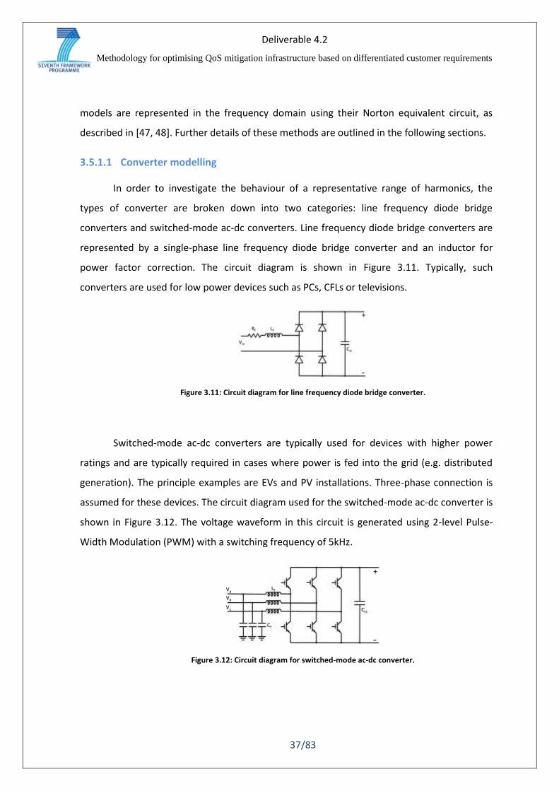
3.5.1.4 Iterative process

The model is run at each frequency in the considered range. For each node and at

each harmonic frequency, the phase of the voltage distortion is recorded and used to adjust

the Norton equivalent impedance of the line frequency diode bridge converter models at that

Node Load (kW)

R1 200

R11 15

R15 52

R16 55

R17 42

R18 47

Lighting 27%

PCs 12%

TV 20%

Routers and Phones 1%

Wet Appliances 1%

Cooking 8%

Cold Appliances 13%

EVs 18%

Deliverable 4.2


43/83

node. This results in an iterative process which gives the final result of the harmonic power

flow at each frequency.

3.5.2 Harmonic power flow results

The key results are the system losses and total harmonic distortion. The total losses

by category are shown in Table 3.8. The total harmonic distortion at each node to which load

is connected is shown in Table 3.9.

Table 3.8: System losses by category.

Current Losses (kW)

All 11.00

Load (50 Hz) 7.44

Harmonics 3.56

3rd-41st Harmonic 3.56

97th-302nd Harmonic 7.85E-05

3rd Harmonic 2.42

5th Harmonic 0.83

7th Harmonic 0.23

3rd Harmonic Neutral 1.82

Table 3.9: Voltage THD at each node with connected load.

Node THD phase a THD phase b

R1 0.00% 0.00%

R11 1.54% 1.77%

R15 3.62% 3.88%

R16 3.47% 3.95%

R17 4.32% 4.94%

R18 4.51% 5.15%

The breakdown of the voltage distortion for phases a and b (phase c is almost

identical to phase a) for a selection of frequencies for the node with the highest THD (node

R18) are shown in Table 3.10.

Deliverable 4.2


44/83

Table 3.10: Voltage distortion at node with highest THD (R18).

Harmonic Order Phase a Voltage Distortion as % of

Fundamental Phase b Voltage Distortion as % of

Fundamental

3 1.73% 3.15%

5 3.31% 3.21%

7 2.05% 2.00%

9 0.28% 0.59%

11 0.85% 0.85%

13 0.90% 0.84%

15 0.17% 0.22%

17 0.32% 0.31%

19 0.46% 0.47%

3.5.3 Discussion

Losses caused by harmonics are 48% of the losses caused by the 50Hz current. The

losses caused by the 3rd harmonic are 68% of the total harmonic losses. This results from the

loading of the neutral cable by the 3rd harmonic. The 3rd harmonic losses in the neutral alone

are more than all the other harmonic losses combined.

Losses at frequencies from the 97th harmonic and higher are minimal, in spite of the

higher cable resistance at these frequencies. There are two reasons. First, emissions are

lower at these higher order harmonics than for low order harmonics. Secondly, the inductive

reactance of the cables in the network is very large at these frequencies and the currents

therefore circulate in the lower impedance paths provided by the capacitances connected

locally at each node.

Voltage distortion increases with distance from the point of connection to the MV

network (main bus). This is to be expected as harmonic current flowing through the network

impedance results in the voltage distortion and the network impedance between node and

main bus increases with distance.

Considering the voltage distortion in phase a and c, it is highest for the 5th harmonic,

although the system current is lower for the 5th than the 3rd harmonic. This results from the

higher inductive reactance of the cables at 250 Hz compared to 150 Hz.

Deliverable 4.2


45/83

In phase b, the 3rd harmonic voltage distortion is significantly higher than for phases a

and c. This is true for all zero-sequence harmonics and results in a significantly greater THD in

phase b. The reason is that the zero-sequence inductance in phase b is larger for the third

harmonic than that in phase a and c. This can be seen in Figure 3.17 and is caused by the

geometry of the cable in which phase b is located further from the return conductor (in this

case the neutral) than phases a and c (which have near identical results).

Assuming a voltage THD limit of 5%, the voltage THD must be mitigated, while losses

are high and should also be addressed. Sections 4.3 and 6.4 address mitigation.

Deliverable 4.2


46/83

4 Effectiveness of PQ Mitigation

The first part of this section investigates the mitigation effect of FACTS devices on

various PQ phenomena (including voltage sags, harmonics and unbalance) Evaluation

methodologies/indices BPI, THD and VUF are applied in the study. The detailed analysis of the

mitigation effectiveness of network-based solutions can be found in [25]. In the second part

of the section harmonic mitigation and suppression of harmonic emission in LV networks is

presented and discussed.

4.1 PQ mitigation using FACTS devices - small test network

The impact of FACTS devices on various PQ phenomena is studied on a simple test

network first. The test network is given in Figure 4.1, which consists of an external grid

modeled as a PV bus type, two buses and one sensitive load modeled as an impedance with

2MW of rated power.

B1 B2

External Grid

Sensitive

load

Line

Figure 4.1: A simple test network

1) Mitigation of voltage sags

In the dynamic simulation of voltage sags, a 3-phase short-circuit is applied to B1 at

0.1s and cleared at 0.3s. In this case, B2 is exposed to a voltage sag. SVC, STATCOM and DVR

are connected to the network individually to test the dynamic response of voltage at B2

during 0-2s, which includes the periods of pre-fault, during-fault and post-fault. The control

parameters of these devices are tuned to be optimal based on trial-and-error method.

STATCOM used for voltage regulation is denoted as STATCOM-V, and that used for reactive

power compensation is denoted as STATCOM-Q. The compensation ability of SVC, STATCOM-

Q and DVR during the sag event is presented in Figure 4.2 (a), (b) and (c) respectively. Since a

sag is defined as the decrease in voltage magnitude between 0.1 and 0.9 p.u., the threshold

of 0.9 p.u. is marked as a solid black line in Figure 4.2. Under initial condition, the voltage

magnitude at B2 is 1.p.u. Given the ideal initial voltage at B2, STATCOM-V and STATCOM-Q

present similar performance. For SVC and STATCOM, relatively large rating is required to

compensate the voltage to 0.9 p.u., as seen from Figure 4.2 (a) and (b), due to the factor that

B2 is connected to a strong bus which is highly affected by the external grid that is modeled

as PV bus. SVC and STATCOM have similar compensation performance during sag event

providing the same rating is applied. As seen from Figure 4.2, the three FACTS devices present

Deliverable 4.2


47/83

different capabilities of post-fault voltage recovery. As the rating is increased, STATCOM has

severer post-fault voltage oscillation compared to SVC. DVR outperforms SVC and STATCOM

in terms of the obtained dynamic response of voltage. DVR not only compensates the during-

fault voltage as expected, and also recovers the post-fault voltage quickly without

experiencing voltage oscillation.

(a) SVC (b) STATCOM-Q & STATCOM-V

(c) DVR

Figure 4.2: Dynamic response of voltage with FACTS devices

2) Mitigation of harmonics

The mitigation of harmonics using various FACTS devices is studied by injecting

harmonic current to the sensitive load. The parameters of the injected harmonic current are

given in Table 4.1. The THD performance obtained with various FACTS devices is given in

Table 4.2. It can be seen that STATCOM has the best performance in terms of harmonic

mitigation effect among the three FACTS devices. SVC-5MVA has a magnified THD compared

to the case of No FACTS, due to the connection of SVC of 5MVA causing resonance at around

3-order. When the rating of SVC is increased to 150MVA, the corresponding THD

performance is significantly improved compared to the case of SVC-5MVA. As for STATCOM

and DVR, the variation of device rating does not appreciably impact THD.

Table 4.1: Harmonic current injection

Harmonic

Order

IAh/IA

(%)

IBh/IB

(%)

ICh/IC

(%)

θAh-θA

(deg.)

θBh-θB

(deg.)

θBh-θB

(deg.)

3 3.849 5.269 4.766 79.353 123.649 121.960

5 25.286 26.130 15.235 24.325 43.858 169.577

7 10.360 7.527 2.134 38.968 157.14 115.175

9 1.206 3.010 5.576 162.417 89.596 26.130

0 0.2 0.4 0.6 0.8 10.5

1

1.5

2

2.5

Time (s)

Voltage m

agnitude (

p.u

.)

0MVA

5MVA

50MVA

100MVA

150MVA

>200MVA

0.9

0 0.2 0.4 0.6 0.8 10.5

1

1.5

2

2.5

Time (s)

Voltage m

agnitude (

p.u

.)

0MVA

5MVA

50MVA

100MVA

>150MVA

0.9

0 0.2 0.4 0.6 0.8 10.5

1

1.5

2

2.5

Time (s)

Voltage m

agnitude (

p.u

.)

0MVA

0.05MVA

0.25MVA

0.5MVA

0.75MVA

>1MVA

0.9

Deliverable 4.2


48/83

Table 4.2: THD (%) obtained with FACTS devices

No

FACTS

SVC-

15MVA

SVC-

150MVA

STATCOM DVR

THDA at B1 0.95 15.43 1.04 0.08 0.11

THDB at B1 1.19 14.24 1.05 0.10 0.06

THDC at B1 0.63 16.71 1.04 0.05 0.14

THDA at B2 1.11 18.87 1.22 0.09 0.18

THDB at B2 1.39 17.65 1.23 0.12 0.10

THDC at B2 0.73 19.20 1.21 0.06 0.24

3) Mitigation of unbalance

The correction effect of various FACTS devices on unbalance phenomenon is studied

by connecting an unbalance load at B2. The rated power of the three phases of the sensitive

load (connected as 3PH-Delta) is given in Table 4.3. In the study, the SVS component of SVC is

equipped with unbalanced controller. PWM is modeled as three-phase converter. The results

are given in Table 4.4. DVR does not impact the VUF at upstream buses. However it increases

the VUF slightly at downstream buses, due to the positive-sequence voltage is used as the

reference for the controller in DVR. To improve this, independent phase controller (i.e., phase

voltage compensation) can be applied. However this approach is not preferred in practice,

due to this requires constantly withdrawing unbalance current from the DC capacitor which

will cause the reduced working life of the capacitor. Besides that, cost will be increased due

to the adoption of more complicated three relatively independent full bridges in PWM [54]. In

the study, DVR is not developed for the purpose of unbalance mitigation.

Table 4.3: Parameters for unbalance load at B2

Phase A Phase B Phase C

Active power (MW) 0.9 0.6 0.8

Power factor 0.3 0.8 0.9

Table 4.4: VUF performance by various FACTS devices

None SVC STATCOM-

50MVA

STATCOM-

150MVA

DVR

VUF at B1 (%) 0.98 0 0.23 0.13 0.98

VUF at B2 (%) 1.18 0 0.28 0.16 1.66

4.2 PQ mitigation using FACTS devices - generic distribution

network

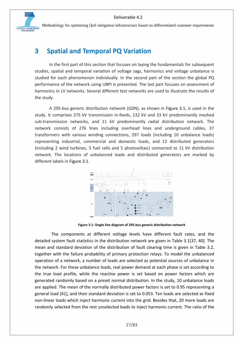
The impact of FACTS devices on various PQ phenomena is further tested in a relatively

practical large-scale distribution network, a 295-bus generic distribution network (GDN), as

shown in Figure 4.3.

Deliverable 4.2


49/83

24

46

17

28

16

14

12

26

21 19

23

223 22

18

15

54

52

53

230

50

75

228

74

229

20221

51 76

13

268

87

48 47

49222

43

42

41

40

39

38

37

269

235 236

231

78

79

80

81

85

88

290

82

83

84

291

91

92

93

95

94

96

97 98

101 99

100

102

103 104

105

106 107

108

109

110

111

112

113

114 115

116

121

122

123124

125

126

127

128

117

118

119 120

86

11

10

8

9

7

6

5

4

55

1 65

64

66 63

57

226 227

58

149

147

154

155

150 153 156

148 146

145

141

143

142

144

140

139

129

130133

131

135

137 136

138

134

157

161

158

186

184

132

160

165

162

163

164

166

167

168169

170

180

181

182 183

185

187

188

189

190 191

192

193

194

197

198

200 199

201

202

203 204

205

206

207

208209

151

152

224

232

77

159

225

215

216

211

212210

213

214

217

218 171

219

220

172

173

174

175

176

177

178

62

60

59

61

2

3

72

70

179

25

27

29

30

32

31 33

3435

36

7168

67 69

73

89

45

44

249 250

266267

242

252

260

289

237

244

261

251

241 245246 243

262272270253 274271 276 275 263 264 273

240

254258 256259

277

247

278

248

280

234

279

233255257

293 292

294 295 297 296

299 298

300

77238

288

269

287 285286

56

BA C D E

F

H I J K L

ON

G

132kV

33kV

11kV

3.3kV

275kV

400kV

G

H2 O2

PV

H2 O2

H2 O2

H2 O2

PV

PV

PV

PV

H2 O2

195

196

H2 O2

PV

Wind Turbine

Photovoltaic

Fuel Cell

Unbalance Load

Zone-1 Zone-2 Zone-3

Figure 4.3: Single line diagram of 295-bus generic distribution network

STATCOM and SVC devices are placed at bus 217, and DVR is connected on the line

between buses 216 and 217. For the convenience of comparison, only one representative

operating point is used, and only one device is activated at one time. The parameters of

FACTS devices are tuned to be optimal. In Figure 4.3, the two branches following bus 217 are

denoted as feeders 1 and 2 respectively.

The compensation effect of various devices on voltage sags is studied by creating a

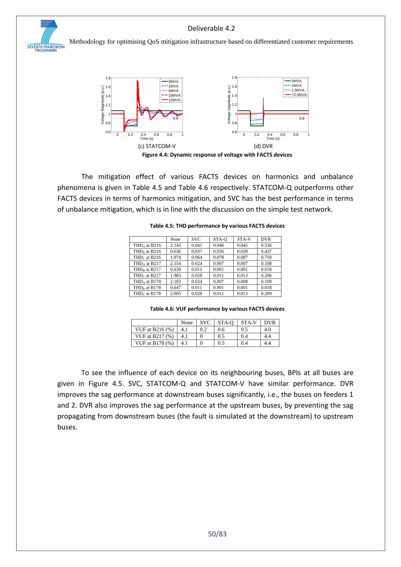
fault at bus 178. The dynamic response of voltage at bus 217 during simulation is given in

Figure 4.4. Without the connection of any FACTS device, the steady state voltage at bus 217 is

larger than 1 p.u. With the connection of STATCOM-V, SVC or DVR, the pre-fault voltage is 1

p.u. When STATCOM-Q is connected, the pre-fault voltage is similar to that obtained without

the connection of any device, as seen from Figure 4.4 (b). Although STATCOM-Q and

STATCOM-V perform similarly during fault, they present different post-fault voltage recovery

ability. In the post-fault period, the performance of STATCOM-Q and STATCOM-V is similar

when the rating is small. However, as the rating increases, STATCOM-V results in more

serious voltage oscillation compared to STATCOM-Q. SVC also suffers from post-fault voltage

oscillation when the rating is increased. In the case of generic distribution network, SVC,

STATCOM-Q and STATCOM-V have the limitation of compensation cap, and they are not able

to compensate the voltage up to 0.9 p.u. In this case, DVR provides much better voltage

dynamic response at B217: it is able to compensate the voltage up to 1 p.u.; and it does not

lead to any post-fault voltage oscillation.

(a) SVC (b) STATCOM-Q

216

217

218 171

219

220

172

173

174

175

176

177

178

0 0.2 0.4 0.6 0.8 10.6

0.8

1

1.2

1.4

1.6

1.8

Time (s)

Voltage m

agnitude (

p.u

.)

0MVA

1MVA

5MVA

10MVA

12MVA

0.9

0 0.2 0.4 0.6 0.8 10.6

0.8

1

1.2

1.4

1.6

1.8

Time (s)

Voltage m

agnitude (

p.u

.)

0MVA

1MVA

5MVA

10MVA

12MVA

0.9

Deliverable 4.2


50/83

(c) STATCOM-V (d) DVR

Figure 4.4: Dynamic response of voltage with FACTS devices

The mitigation effect of various FACTS devices on harmonics and unbalance

phenomena is given in Table 4.5 and Table 4.6 respectively. STATCOM-Q outperforms other

FACTS devices in terms of harmonics mitigation, and SVC has the best performance in terms

of unbalance mitigation, which is in line with the discussion on the simple test network.

Table 4.5: THD performance by various FACTS devices

None SVC STA-Q STA-V DVR

THDA at B216 2.143 0.041 0.046 0.045 0.536

THDB at B216 0.636 0.037 0.026 0.028 0.437

THDC at B216 1.974 0.064 0.078 0.087 0.759

THDA at B217 2.154 0.024 0.007 0.007 0.108

THDB at B217 0.639 0.011 0.001 0.001 0.018

THDC at B217 1.983 0.028 0.011 0.013 0.206

THDA at B178 2.183 0.024 0.007 0.008 0.109

THDB at B178 0.647 0.011 0.001 0.001 0.018

THDC at B178 2.005 0.028 0.011 0.013 0.209

Table 4.6: VUF performance by various FACTS devices

None SVC STA-Q STA-V DVR

VUF at B216 (%) 4.1 0.2 0.6 0.5 4.0

VUF at B217 (%) 4.1 0 0.5 0.4 4.4

VUF at B178 (%) 4.1 0 0.5 0.4 4.4

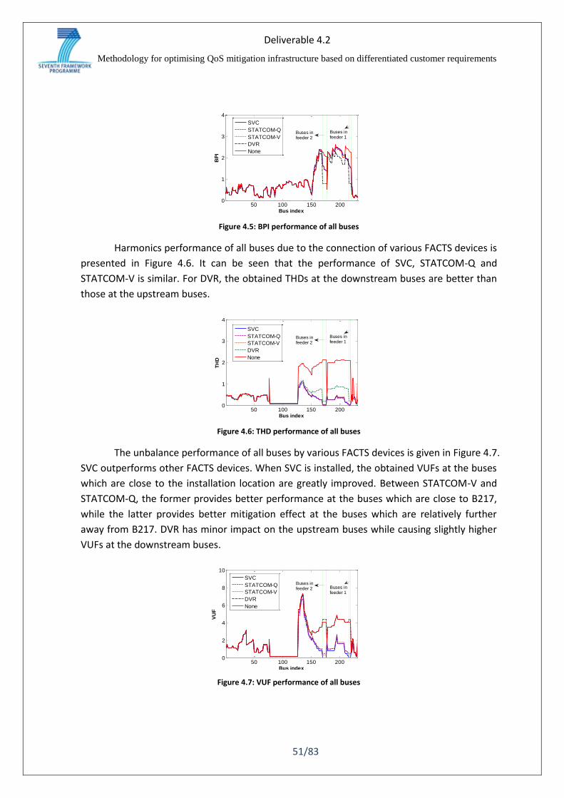
To see the influence of each device on its neighbouring buses, BPIs at all buses are

given in Figure 4.5. SVC, STATCOM-Q and STATCOM-V have similar performance. DVR

improves the sag performance at downstream buses significantly, i.e., the buses on feeders 1

and 2. DVR also improves the sag performance at the upstream buses, by preventing the sag

propagating from downstream buses (the fault is simulated at the downstream) to upstream

buses.

0 0.2 0.4 0.6 0.8 10.6

0.8

1

1.2

1.4

1.6

1.8

Time (s)

Voltage M

agnitude (

p.u

.)

0MVA

1MVA

5MVA

10MVA

12MVA

0.9

0 0.2 0.4 0.6 0.8 10.6

0.8

1

1.2

1.4

1.6

1.8

Time (s)

Voltage m

agnitude (

p.u

.)

0MVA

1MVA

2.5MVA

>5.5MVA

0.9

Deliverable 4.2


51/83

Figure 4.5: BPI performance of all buses

Harmonics performance of all buses due to the connection of various FACTS devices is

presented in Figure 4.6. It can be seen that the performance of SVC, STATCOM-Q and

STATCOM-V is similar. For DVR, the obtained THDs at the downstream buses are better than

those at the upstream buses.

Figure 4.6: THD performance of all buses

The unbalance performance of all buses by various FACTS devices is given in Figure 4.7.

SVC outperforms other FACTS devices. When SVC is installed, the obtained VUFs at the buses

which are close to the installation location are greatly improved. Between STATCOM-V and

STATCOM-Q, the former provides better performance at the buses which are close to B217,

while the latter provides better mitigation effect at the buses which are relatively further

away from B217. DVR has minor impact on the upstream buses while causing slightly higher

VUFs at the downstream buses.

Figure 4.7: VUF performance of all buses

50 100 150 2000

1

2

3

4

Bus indexB

PI

SVC

STATCOM-Q

STATCOM-V

DVR

None

Buses infeeder 2

Buses infeeder 1

50 100 150 2000

1

2

3

4

Bus index

TH

D

SVC

STATCOM-Q

STATCOM-V

DVR

None

Buses infeeder 2

Buses infeeder 1

50 100 150 2000

2

4

6

8

10

Bus index

VU

F

SVC

STATCOM-Q

STATCOM-V

DVR

None

Buses infeeder 1

Buses infeeder 2

Deliverable 4.2


52/83

4.3 Harmonic mitigation in LV Network

Following the modelling in section 3.5, harmonic mitigation in the case study of the

CIGRE LV Benchmark Network is carried out.

Three mitigation methods are considered. The first, which is the lowest cost existing

solution and primarily used as a benchmark, is the addition of tuned passive filters to the

network to reduce voltage THD. The second is to consider the effect of distributed harmonic

compensation, which can be provided as an ancillary service by distributed energy resources

that are interfaced to the network with a switched-mode ac-dc converter [55-57]. The

strategy is to use the switched-mode ac-dc converters to produce harmonics in anti-phase to

emissions from line frequency diode bridge converters, effectively absorbing those emissions.

The method has the same principle as active filter operation, but avoids the cost of a

dedicated filter. The third method is to replace line frequency diode bridge converters with

switched-mode ac-dc converters.

The intention is to establish an economic framework in which the costs of installing

filters are avoided and losses reduced by providing incentives to owners of grid connected

equipment to either reduce their harmonic emissions or compensate harmonic emissions;

this is examined further in section 6.4.

4.3.1 Passive filters

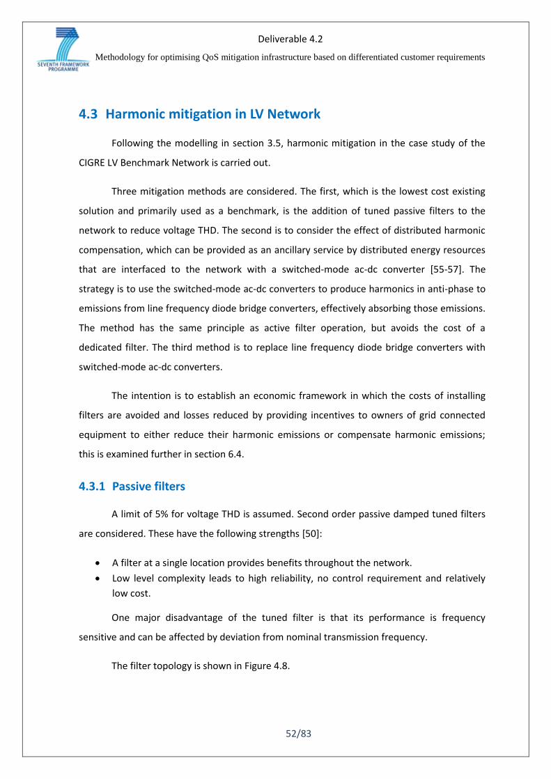
A limit of 5% for voltage THD is assumed. Second order passive damped tuned filters

are considered. These have the following strengths [50]:

A filter at a single location provides benefits throughout the network.

Low level complexity leads to high reliability, no control requirement and relatively

low cost.

One major disadvantage of the tuned filter is that its performance is frequency

sensitive and can be affected by deviation from nominal transmission frequency.

The filter topology is shown in Figure 4.8.

Deliverable 4.2


53/83

Figure 4.8: Second order damped shunt filter.

It was found that the most effective placement for the filter(s) was at the node with

highest voltage THD (node R18). Installation of a 3rd harmonic filter was found to be

problematic. The reduction in the 3rd harmonic voltage leads to an increase in the 3rd

harmonic current drawn by devices. This is because the voltage distortion at a given harmonic

acts to reduce the current drawn at that frequency. In the case of the 3rd harmonic, the extra

current drawn returns in the neutral path and further increases the largest source of

harmonic losses.

A filter for the 5th harmonic was therefore modelled. It was found that a tuned 5th

harmonic filter was adequate to reduce the voltage THD in phase b to below 5%. In addition,

losses at the 5th harmonic are reduced because a large proportion of these currents are now

drawn from the filter rather than the connection point to the MV network and therefore flow

through a shorter cable length. The voltage THD at each node for phases a and b, before and

after filtering are shown in Table 4.7.

Table 4.7: Voltage THD mitigation by use of tuned filters.

Base Case 5th Harmonic Filter

Only 5th and 7th Harmonic

Filters

Node Phase a Phase b Phase a Phase b Phase a Phase b

R1 0.00% 0.00% 0.00% 0.00% 0.00% 0.00%

R11 1.54% 1.77% 1.19% 1.50% 1.03% 1.37%

R15 3.62% 3.88% 3.09% 3.44% 2.87% 3.26%

R16 3.47% 3.95% 2.61% 3.27% 2.19% 2.97%

R17 4.32% 4.94% 3.04% 3.94% 2.37% 3.48%

R18 4.51% 5.15% 3.06% 4.04% 2.28% 3.52%

Deliverable 4.2


54/83

4.3.2 Distributed harmonic compensation and reduction of harmonic

emission

In order to assess a fair price for a scheme to incentivise customers to reduce or

mitigate harmonics, it is necessary to establish what level of loss and voltage THD mitigation

is achieved for a given amount of harmonic mitigation. This depends on spatial

considerations, i.e. reduction of harmonics at certain nodes is more effective than at others.

In order to do this, the marginal effect on voltage THD throughout the system and system

losses of reducing harmonics at each node is measured. The results are shown in Table 4.8

and Table 4.9. In order to normalise the results, the mitigation is assumed to be equivalent to

the harmonic spectrum of a device drawing 100 W, with harmonic spectrum as shown in

Figure 3.13, in each phase.

Table 4.8: Effect on system losses of harmonic mitigation equivalent to harmonic spectrum for 100 W device with line frequency diode bridge converter grid interface in each phase.

Node with Mitigation

Distance from Main Bus (m)

Loss Mitigation for Harmonic Load Reduction (W)

Loss Mitigation for Harmonic

Compensation (W)

R1 0 0 0

R11 90 1.04 1.13

R15 240 2.21 2.70

R16 205 1.99 2.28

R17 310 2.14 2.48

R18 345 2.59 2.94

Table 4.9: Reduction of voltage THD of harmonic mitigation equivalent to harmonic spectrum for 100 W device with line frequency diode bridge converter grid interface in each phase. Results for phase b are shown.

THD Measured at

Node

Compensated Node

R1 R11 R15 R16 R17 R18

R1 0.0000% 0.0000% 0.0000% 0.0000% 0.0000% 0.0000%

R11 0.0000% 0.0115% 0.0052% 0.0055% 0.0053% 0.0053%

R15 0.0000% 0.0045% 0.0283% 0.0068% 0.0065% 0.0064%

R16 0.0000% 0.0045% 0.0058% 0.0182% 0.0124% 0.0123%

R17 0.0000% 0.0041% 0.0052% 0.0116% 0.0260% 0.0203%

R18 0.0000% 0.0038% 0.0048% 0.0107% 0.0244% 0.0186%

Deliverable 4.2


55/83

An example in order to explain Table 4.9 follows. Consider node R15. The voltage THD

at this node before any compensation is 3.88%. Compensation can be provided anywhere in

the network (compensating one node affects all nodes). Providing compensation at node R11,

equivalent to mitigating emissions from a 100 W line frequency diode bridge converter,

reduces the voltage THD at node R15 by 0.0052%. Similar results are true when

compensation is provided at nodes R16, R17 or R18. Providing the same compensation at

node R15 itself reduces voltage THD at the node by 0.0283%, i.e. it is much more effective.

Voltage distortion mitigation is most effective when carried out at or close to nodes

that have the greatest voltage THD. It can be seen that harmonic reduction at the load

connected directly to the main bus does little to mitigate harmonic effects. Loss mitigation is

most effective when carried out far from the main bus.

The methods of compensation and reduction have the additional advantage that they

are not affected by deviations from nominal system frequency. In the case of compensation,

the switched-mode ac-dc converter automatically responds to changes in system frequency.

Deliverable 4.2


56/83

5 PQ Mitigation Planning based on Technical

performance of the network

5.1 Optimisation methodology

With mitigation options (both FACTS devices and network-based solutions), an

optimal deployment methodology for mitigation solutions has to be applied to identify the

most appropriate type of mitigation, rating of devices, location of their placement in network

based on the objectives of minimising PQ severity indices (or minimising deviation from

guaranteed quality levels for each category of customers, which will be introduced later). In

the study, the objective function, F, which is to evaluate the mitigation solutions, is defined

as:

𝐹(𝑥) = ∑ (𝑈𝐵𝑃𝐼𝑖(𝑥))𝑖 subject to: 𝑔(𝑥) = 0, ℎ(𝑥) ≥ 0 (5.1)

where x denotes the variables to be optimised, i.e. the mitigation solutions, which consist of

the location, type and size of various FACTS devices and network-based solutions; 𝑔(𝑥) = 0

and ℎ(𝑥) ≥ 0 denote the equality and inequality constraints respectively. It can be seen that

with the sum of the unified indices of all buses, objective function F reflects the severity of

three phenomena throughout the whole network.

5.1.1 Identification of feasible locations for deployment of mitigating

solutions

In order to optimally deploy mitigating solutions , potential and effective locations are

initially identified. The locations selected for the application of network-based solutions are

mainly based on the ranking of buses according to BPI, VUF and THD, together with the

network resources and geographical constraints. The locations for installing FACTS devices

are selected based on PQ performance and sensitivity analysis. Firstly, buses are sorted

according to BPI, VUF, THD, ∑ |𝜕𝑉𝑗

𝜕𝑄|

𝑁𝐵𝑗=1 and ∑ |

𝜕𝑉𝑗

𝜕𝑃|

𝑁𝐵𝑗=1 in descending order, respectively. The

ranking index of bus i with respect to BPI is denoted as RBPI(Bi), and the same applies to other

variables. Then RBPI(Bi)=1 suggests that bus i is experiencing the worst sag performance, and

𝑅𝜕𝑉/𝜕𝑄(𝐵𝑖) = 1 that voltage of bus i is the most sensitive to the injection of reactive power.

With these rankings, the potential locations are chosen globally (i.e., based on the whole

network) and zonally (i.e., based on zones information) respectively.

The buses having RBPI=1, RVUF=1, the smallest 𝑅BPI + 𝑅𝜕𝑉/𝜕𝑄, the smallest 𝑅VUF +

𝑅𝜕𝑉/𝜕𝑄 and the smallest RBPI+𝑅VUF are selected as potential locations for installing SVC.

Following this appropriate FACTS devices are preliminarily paced at the selected potential

locations, the same selection procedure is then performed again to select the second set of

Deliverable 4.2


57/83

potential placements. The aforementioned procedure is applied to select the potential

locations for installing STATCOM and DVR, while in this case the buses having RBPI=1, RVUF=1,

the smallest 𝑅BPI +𝑅𝜕𝑉/𝜕𝑃 +𝑅𝜕𝑉/𝜕𝑄

2, the smallest 𝑅VUF +

𝑅𝜕𝑉/𝜕𝑃 +𝑅𝜕𝑉/𝜕𝑄

2 and the smallest

RBPI+𝑅VUF are selected. Instead of using 𝑅𝜕𝑉/𝜕𝑄, 𝑅𝜕𝑉/𝜕𝑃 +𝑅𝜕𝑉/𝜕𝑄

2 is used in this case as both

STATCOM and DVR can transmit both active and reactive power between devices and the

grid.

To ensure the capability of providing specific quality of supply required in a particular

zone, the potential locations should be also selected zonally. In the zonal selection, the

procedure is the same as the global selection, except that the ranking procedure is performed

within the zones rather than within the whole network.

Geography feasibility could be also taken into account during the process of selecting

potential locations. The same aforementioned selection procedure is performed to select the

potential locations for installing passive filters, while in this case the buses are ranked based

on RTHD. Besides, the intersection of two branches which have more than three buses in

downstream branches is also initially made available for placement of passive filters, as the

passive filters located at the intersection of two branches can stop the harmonic current

flowing to other branches.

5.1.2 Optimisation methodology

With these pre-selected locations, greedy algorithm is used to search the potential

solutions (i.e., optimal placement of FACTS devices and their optimal rating settings) to

minimise the gap between PQ performance achieved and the PQ thresholds. Greedy

algorithm is chosen due to its simplicity of implementation and computation efficiency. It

divides the problem into different consecutive stage and solves the problem heuristically by

making the local optimal choice ‘greedily’ at each stage. The greedy algorithm has been

applied successfully for device placement in large scale power systems.

Before applying the greedy algorithm, a pool of potential solutions, denoted as set U,

should be determined based on the initial placement/locations and rating constraints. For

FACTS devices, their initial placements including their location and type have been decided.

Assume there are MD potential devices. For each potential device, an extra variable needs to

be determined, i.e. the rating of the device. The rating range of each device can be divided

into MI intervals, and for each interval, a rating is chosen by randomly selecting a value within

the interval. Thus, a pool of MD×MI potential devices, which consists of locations, types of

devices and ratings, and a number of network-based solutions, denoted as set U are made

available initially for optimisation process.

Deliverable 4.2


58/83

Figure 5.1: Flowchart of greedy algorithm

After the solution pool U and objective function are defined, a conventional

methodology, Greedy Algorithm, which is widely applied to solve the travelling salesman

problem (TSP), is applied to optimise the mitigation variables of FACTS devices. The greedy

algorithm solves the problem heuristically by making the local optimal choice ‘greedily’ at

each stage, until the stop criteria is reached. The choice made by the algorithm depends on

the choices so far instead of the future choices. In other words, it chooses the optimal

solutions of sub-problems derived along the selection process. In our study, a certain number

of stages are applied for the placement of FACTS devices. The Greedy Algorithm is applied at

each stage where only one FACTS device which has the best mitigation effect is chosen. The

choice is made after all unselected FACTS devices with various proposed ratings are tested

individually. The reason for repeatedly testing all the unselected FACTS devices is that the

operation condition varies due to the integration of selected devices, and the mitigation

effect of mitigation devices would vary as well, even though the same device with the same

rating is applied. The repeating device selection stops if the improvement to the objective

function between two neighbouring stages is smaller than a pre-set value. The flowchart of

the application of greedy algorithm for this allocation problem is given in Figure 5.1, where s is

the chosen solution which is corresponding to the minimum SGI at each stage; Γ denotes the

devices selected so far; and X is the updated pool of potential solutions at each stage. At each

stage, X is updated by removing its elements which have the same location and type of devise

as the selected s. The optimisation procedure can be terminated if the size of Γ reaches the

preset maximum number of devices allowed to be installed, or if the improvement of PQ

performance between two sequential stages is smaller than a preset threshold. Set Γ is

selected as the final optimal mitigation solutions.

To test this methodology, UBPI is taken as the objective function to be minimised by

Begin

X=U; Γ=Φ;

End

Select sϵX that minimizes

objective function;

X=X-{all elements in X which have the

same location and type of device as s};

Γ=Γ∪{s};

Reach stop criteria?

Input set U of

potential devices

Yes

No

Install covered devices Γ;

Update X by regenerate rating randomly

within corresponding interval

Deliverable 4.2


59/83

the proposed methodology. The convergence characteristic of the optimisation methodology

is presented in Figure 5.2 (a), which shows that the sum of UBPIs in the network is greatly

reduced when one mitigation technique is applied, and the performance is steadily improved

when the number of installed devices>4. The UBPIs obtained at all buses are given in Figure

5.2 (b), which shows that the UBPI is significantly improved with mitigation solutions. To

visually present the improvement of PQ performance, the heat-maps of UBPIs obtained

without and with mitigation are given in Figure 5.3 (a) and (b) respectively. It can be seen that

the critical areas which are exposed to the PQ disturbance are greatly improved.

(a) Convergence curves (b) UBPI obtained with and without mitigation

Figure 5.2: UBPIs of all buses and convergence characteristic of the optimisation methodology

149

147

154

155

150 153 156

148 146

145

141

143

142

144

140

139

129

130 133

131

135

137 136

138

134

157

161

158

186

184

132

160

165

162

163

164

166

167

168169

170

180

181

182 183

185

187

188

189

190 191

192

193

194

197

198

200 199

201

202

203 204

205

206

207

208209

151

152

224

232

77

159

225

215

216

211

212210

213

214

217

218 171

219

220

172

173

174

175

176

177

178

265

195

196

L

24

46

17

28

16

14

12

26

21 19

23

223 22

18

15

54

52

53

230

50

75

228

74

229

20221

51 76

13

268

87

48 47

49222

43

42

41

40

39

38

37

269

231

78

79

80

81

85

88

290

82

83

84

291

91

92

93

95

94

96

97 98

101 99

100

102

103 104

105

106 107

108

109

110

111

112

113

114 115

116

121

122

123124

125

126

127

128

117

118

119 120

86

11

10

8

9

7

6

5

4

55

1 65

64

66 63

57

226 227

58

62

60

59

61

2

3

72

70

179

25

27

29

30

32

31 33

3435

36

7168

67 69

73

89

45

44

266267

289

238

288

269

287 285286

56

BA C D E H I J K

26426326033kV

11kV

H2 O2

Non-linear load (fixed)

Photovoltaic

Fuel Cell

Wind Turbine

Unbalance load (fixed)

(a) without mitigation

149

147

154

155

150 153 156

148 146

145

141

143

142

144

140

139

129

130 133

131

135

137 136

138

134

157

161

158

186

184

132

160

165

162

163

164

166

167

168169

170

180

181

182 183

185

187

188

189

190 191

192

193

194

197

198

200 199

201

202

203 204

205

206

207

208209

151

152

224

232

77

159

225

215

216

211

212210

213

214

217

218 171

219

220

172

173

174

175

176

177

178

265

195

196

L

24

46

17

28

16

14

12

26

21 19

23

223 22

18

15

54

52

53

230

50

75

228

74

229

20221

51 76

13

268

87

48 47

49222

43

42

41

40

39

38

37

269

231

78

79

80

81

85

88

290

82

83

84

291

91

92

93

95

94

96

97 98

101 99

100

102

103 104

105

106 107

108

109

110

111

112

113

114 115

116

121

122

123124

125

126

127

128

117

118

119 120

86

11

10

8

9

7

6

5

4

55

1 65

64

66 63

57

226 227

58

62

60

59

61

2

3

72

70

179

25

27

29

30

32

31 33

3435

36

7168

67 69

73

89

45

44

266267

289

238

288

269

287 285286

56

BA C D E H I J K

26426326033kV

11kV

H2 O2


Photovoltaic

Fuel Cell

Wind Turbine


Non-linear load (random)

FACTS_based mitigation

(b) with mitigation

Figure 5.3: Illustration of the performance of the proposed optimisation methodology

5.2 Simulation results

The developed optimisation methodology introduced above is used to search the

optimal mitigation solutions to provide differentiated levels of PQ in the 295-GDS distribution

network. The GDS is divided into three zones, as shown in Figure 5.4. The comparison

between UBPIs obtained with and without mitigation solutions is presented in Figure 5.5 (a),

0 2 4 6 8 10 120

20

40

60

80

100

Number of installed Devices

Sum

(UB

PI i)

(H

arm

onic

, S

ag, U

nbala

nce)

0 50 100 150 200 2500

0.5

1

1.5

2

2.5

Bus No

UB

PI (H

arm

onic

, S

ag, U

nbala

nce)

Without mitigation with H5S3U2

With mitigation with H5S3U2

Deliverable 4.2


60/83

and the convergence characteristic of UBPI against the number of installed devices is given in

Figure 5.5 (b). Figure 5.6 presents the heatmaps of annual PQ performance obtained without

and with mitigation. It can be seen that the performance is significantly improved with the

optimal mitigation solutions found by the developed methodology. Furthermore, the

heatmaps obtained from the concerned operating points (corresponding the maximum load

and maximum cluster) are given in Figure 5.7. Compared to Figure 3.8, PQ performance

presented in Figure 5.7 is greatly improved.

Figure 5.4: The illustration of zone division

(a) UBPIs obtained with and without mitigation (b) Convergence curves

Figure 5.5: Illustration of the performance of the proposed methodology for provisioning differentiated QoS

149

147

154

155

150 153 156

148 146

145

141

143

142

144

140

139

129

130 133

131

135

137 136

138

134

157

161

158

186

184

132

160

165

162

163

164

166

167

168169

170

180

181

182 183

185

187

188

189

190 191

192

193

194

197

198

200 199

201

202

203 204

205

206

207

208209

151

152

224

232

77

159

225

215

216

211

212210

213

214

217

218 171

219

220

172

173

174

175

176

177

178

265

195

196

L

24

46

17

28

16

14

12

26

21 19

23

223 22

18

15

54

52

53

230

50

75

228

74

229

20221

51 76

13

268

87

48 47

49222

43

42

41

40

39

38

37

269

231

78

79

80

81

85

88

290

82

83

84

291

91

92

93

95

94

96

97 98

101 99

100

102

103 104

105

106 107

108

109

110

111

112

113

114 115

116

121

122

123124

125

126

127

128

117

118

119 120

86

11

10

8

9

7

6

5

4

55

1 65

64

66 63

57

226 227

58

62

60

59

61

2

3

72

70

179

25

27

29

30

32

31 33

3435

36

7168

67 69

73

89

45

44

266267

289

238

288

269

287 285286

56

BA C D E H I J K

26426326033kV

11kV

H2 O2


Photovoltaic

Fuel Cell

Wind Turbine



149

147

154

155

150 153 156

148 146

145

141

143

142

144

140

139

129

130 133

131

135

137 136

138

134

157

161

158

186

184

132

160

165

162

163

164

166

167

168169

170

180

181

182 183

185

187

188

189

190 191

192

193

194

197

198

200 199

201

202

203 204

205

206

207

208209

151

152

224

232

77

159

225

215

216

211

212210

213

214

217

218 171

219

220

172

173

174

175

176

177

178

265

195

196

L

24

46

17

28

16

14

12

26

21 19

23

223 22

18

15

54

52

53

230

50

75

228

74

229

20221

51 76

13

268

87

48 47

49222

43

42

41

40

39

38

37

269

231

78

79

80

81

85

88

290

82

83

84

291

91

92

93

95

94

96

97 98

101 99

100

102

103 104

105

106 107

108

109

110

111

112

113

114 115

116

121

122

123124

125

126

127

128

117

118

119 120

86

11

10

8

9

7

6

5

4

55

1 65

64

66 63

57

226 227

58

62

60

59

61

2

3

72

70

179

25

27

29

30

32

31 33

3435

36

7168

67 69

73

89

45

44

266267

289

238

288

269

287 285286

56

BA C D E H I J K

26426326033kV

11kV

H2 O2


Photovoltaic

Fuel Cell

Wind Turbine


DVR

SVC

STATCOM

PF

(b) with mitigation

Figure 5.6: Heatmaps of annual PQ performance obtained with 6 devices in case 4 with and without mitigation

0 50 100 150 200 2500

0.2

0.4

0.6

0.8

1

1.2

Bus No

UB

PI (H

arm

onic

, S

ag, U

nbala

nce

)

Without mitigation

With mitigation

Error

Zone threshold

2 4 6 8 10 120

20

40

60

80

100

Number of devices installed

Sum

(U

BP

I i) (H

arm

onic

, S

ag, U

nbala

nce)

Deliverable 4.2


61/83

(a) Maximum cluster

(b) Maximum load

Figure 5.7: Heat maps of the concerned operating points with optimal mitigation solution based on UBPI

Time series simulations are adopted to validate the selected solutions of PQ. 24 hours

simulations for a selected day were performed. The results are shown in Figure 5.8, as it can

be seen few buses violate the requirements of the zone at some hours even after mitigation.

However, the common measures for long periods of studies are the percentiles, in particular

the 95th percentile, therefore these levels of performance can be accepted based on the

commonly adopted standards and regulations. Moreover, the requirements are also variable

with time, and the adopted thresholds are the most conservative and the tightest thresholds

of a probabilistic range of immunity level. In other words these thresholds (acceptable

immunity levels) can be more relaxed at some hours of the day (due to different load mix at

these hours and therefore different participation of sensitive customers) and the

“participating” sensitive customers could survive worse PQ performance at those hours. If the

pessimistic evaluation is to be avoided, probabilistic representation of the thresholds is

required.

Deliverable 4.2


62/83

Figure 5.8: UBPIs obtained without and with mitigation at all buses for 24 hours’ operation

0 50 100 150 2000

0.1

0.2

0.3

0.4

0.5

0.6

0.7

0.8

0.9

1

Bus index

UB

PI

without mitigation

with mitigation

Thresholds

Deliverable 4.2


63/83

6 PQ mitigation Planning Based on Techno-Economic

Analysis

6.1 Methodology for assessment of economic viability of PQ

mitigation solutions

While performing economic assessment of PQ mitigation at planning level, it is

important to consider the benefits during the entire life span of the deployed solution. The

upfront investment made for a mitigation solution pays back its returns only during the life

span duration. This makes it important to consider the net present value of future benefits, as

well as the net present value of future maintenance. This brings the investment cost and its

benefit to a common ground/level of comparison with planning or deployment year as the

reference. This net present value approach accounts for the facts like inflation (denoted as i),

discount rate (denoted as r) and escalation rate (denoted as e) required for the time value of

money. Net present value can be calculated using the following equation:

𝑁𝑃𝑉 = 𝐶𝐼 +∑ (𝐶𝑡𝑏+𝐶𝑡𝑐)×(1+𝑒)𝑡𝑛

𝑡=0

((1+𝑟)(1+𝑖))𝑡 (6.1)

where CI denotes the initial capital investment (usually expressed as a negative amount), Ctb

denotes the benefit component occurring at the beginning of time period; and Ctc denotes

the cost component occurring at beginning of time period t (usually expressed as a negative

amount).

6.1.1 Assessment of financial consequence of PQ phenomena

Detailed analysis of economic impact due to voltage sags, unbalance and harmonics

are very important while considering the investment on mitigation solutions. Economic

impact can be assessed by identifying losses to different types of business due to various PQ

phenomena. Considering the diversity of business types that exists, customers can be

categorized based on their previous history of economic losses due to inadequate PQ issues,

similarities in their business process and the sensitivity of equipment/devices used for their

business. This categorization enables to evaluate the economic impact of a group of

customers using a common model, thus each category having a unique model for analysis.

This economic impact provides an estimate of financial losses for that particular customer for

a given level of PQ in a network. Since losses due to voltage sags, unbalance and harmonics

are due to different reasons, it requires separate financial assessment models for each of

them.

The financial losses to a certain type of customers due to sag events are mainly

Deliverable 4.2


64/83

caused by process trip. For instance，industrial processes (glass production, textile industry) are

very sensitive to sag events [1, 9]. The main elements/parameters that should be considered

when assessing process trip include sag characteristics, frequency of sags at the customer

busbar, equipment sensitivity, customer plant sensitivity, process operational cycle and the

plant’s load profile. In the study, sag characteristics and frequency are simulated using a

stochastic approach which is to comprehensive assessment of the impact of voltage sags in

large scale power networks [37]. With realistic modelling of process cycle and proper

probabilistic modelling of uncertainties associated with each of the influential parameters,

the approach of risk analysis is applied to assess possibility of having industrial process trip.

The financial loss due to a sag event can be assessed by [1]:

(Financial

loss) = (

Process failure risk

) × (Loss due to process trip

) (6.2)

where the loss due to process trip is derived through survey or from customers directly.

Economic losses due to unbalance are mainly caused by power and energy losses and the

shortened life of equipment, according to the general classification of unbalance cost

proposed by CIGRE/CIRED C4.107 report in the context of customers [58]. As far as customers

are concerned the major impact happens in the case of induction motors, and can be

considered as one of the major source of economic losses for them. These losses happens

both due to de-rating of induction motors and loss of useful life. As per NEMA guidelines

induction motors are not expected to operate under condition of unbalance power supply

percentage of above 5%. The guideline recommends de-rating of induction motors in order to

avoid damage of motor. NMEA MG-1 suggests the de-rating curves, which combines

relationships between winding temperature rise with percentage load and winding

temperature rise with voltage unbalance, for calculating power loss in induction motors [59].

The difference in rated power and de-rated power can be considered as loss of power due to

unbalance and can be converted to financial cost. Using the rate of unit cost of energy over a

period of time and applying the NPV method it is possible to identify the accumulated cost of

energy losses over the period of system study. These costs are considered as operating costs

since this gets accounted into the operating expense incurred from payment of electricity

charges by a business.

Customer with business types having substantial installation of induction motors

suffers the most from equipment ageing issues. Equipment ageing due to thermal stress can

modeled as [60, 61]:

𝐿 = 𝐿0′ 𝑒−(𝐵𝑐𝜃) (6.3)

where 𝐿0′ refers to the reference life of the equipment for a reference temperature 𝜃𝑜; B is a

constant for a material represented as B = E/K, where E is the activation energy of the aging

reaction in Joule/mol and K is the gas constant in JK-1mol-1; 𝑐𝜃 =1

𝜃0−

1

𝜃, where 𝜃0 is the

nominal operating temperature of the insulation in sinusoidal regime while 𝜃 is the operating

temperature in the presence of harmonics.

Deliverable 4.2


65/83

As per NMEA-1 guideline the approximate increase in winding temperature ∆𝜃 of

induction motor due to percentage voltage unbalance 𝑉𝑎𝑠 can be calculated using ∆𝜃 = 2𝑉𝑎𝑠2 .

A decrease in useful life of the motor results in economic loss due to equipment replacement

and process disruption due to equipment damage. The financial cost due to equipment age

can be approximated by 𝐿0

′ −𝐿

𝐿× 𝐶𝑟𝑒, where 𝐶𝑟𝑒denotes the cost of replacing the motor.

Financial losses from voltage harmonics and current harmonics can be classified into

border category of energy losses, losses due to premature ageing and losses from equipment

malfunction. CIGRE/CIRED C4.107 report [58] presents methodologies for evaluating

economic losses arising from wave form distortion due to harmonics. The additional power

losses due to harmonics voltages and currents occur as core loss, copper loss and dielectric

losses in electrical equipment. In order to analyse overall costs of an industrial system each of

equipment type has to be considered separately for calculating power losses from individual

type of equipment. The harmonic losses for induction motors can be calculated using [58]:

𝑃𝑀 = 3 ∑ (𝑉ℎ

𝑍𝑀ℎ )

2

𝑅𝑀ℎℎmax

ℎ=ℎ1+ 𝑃𝑐𝑜

1 ∑ (𝑉ℎ

𝑍𝑀ℎ )

𝑚𝑀 1

ℎ0.6

ℎmax ℎ=ℎ1

(6.4)

Where 𝑉ℎ represent the voltage harmonic of order h; 𝑍𝑀ℎ and 𝑅𝑀

ℎ denotes the equivalent

impedance and resistance of the motor at the harmonic of order h respectively; 𝑃𝑐𝑜1 denotes

the core loss at the fundamental frequency; and 𝑚𝑀 is the numerical coefficient.

Harmonic distortions can cause additional electric and thermal stresses in insulating

materials of electric equipment. Additional electric stresses are mainly due to the increased

peak factor of voltage level resulting from the presence of harmonics. Increase in thermal

stress is due to the rise in temperature from additional copper and core losses of equipment

caused by harmonic contents. Additional stresses can cause failure of the equipment

insulation, consequently reducing the equipment life span. Financial losses to customers

occur by replacing the costly equipment and production losses due to unexpected process

failure. A simple electro thermal life model recommended by CIGRE/CIRED C4.107 based on

[60, 61] can be represented as:

𝐿 = 𝐿0′ (𝐾𝑝)

−𝑛𝑝𝑒−(𝐵𝑐𝜃) (6.5)

where 𝐾𝑝 is the peak factor of the voltage waveform represented by 𝐾𝑝 =𝑉𝑝

𝑉1𝑝∗ where 𝑉𝑝 is the

value of the distorted voltage while 𝑉1𝑝∗ is the peak value of fundamental voltage; 𝑛𝑝 is the

coefficient related to the shape of the distorted waveform; and 𝑐𝜃 =1

𝜃0−

1

𝜃. The operating

temperature rise at the hottest point at operating conditions can be evaluated using the

formula of ∆𝜃 ≈ (𝑃ℎ

𝑃0) × ∆𝜃0, where ∆𝜃and ∆𝜃0 represent the operating temperature rise

from ambient in non-sinusoidal operating condition and nominal power 𝑃0 respectively; and

𝑃ℎ is the harmonics content of power.

Deliverable 4.2


66/83

The aforementioned costs due to PQ phenomena can be calculated using Net Present

Value method so that present worth of future economic losses can be identified.

6.1.2 Assessment of financial cost of PQ mitigation

The capital cost of SVC, DVR and PF can be obtained based on curve fitting approach

using available cost records. The costs of DVR and STATCOM are considered as the same. The

capital cost including construction cost of these devices can be defined as [62, 63]:

𝐶𝑆𝑇𝐴𝑇+𝐶𝑜𝑛 = 553(−0.0008𝑆𝑆𝑇𝐴𝑇2 + 0.155𝑆𝑆𝑇𝐴𝑇 + 120) (

£

𝑀𝑉𝐴𝑟) (6.6)

𝐶𝐷𝑉𝑅+𝐶𝑜𝑛 = 553(−0.0008𝑆𝐷𝑉𝑅2 + 0.155𝑆𝐷𝑉𝑅 + 120) (

£

𝑀𝑉𝐴𝑟) (6.7)

𝐶𝑆𝑉𝐶+𝐶𝑜𝑛 = 553(0.0003𝑆𝑆𝑉𝐶2 − 0.3051𝑆𝑆𝑉𝐶 + 127.38) (

£

𝑀𝑉𝐴𝑟) (6.8)

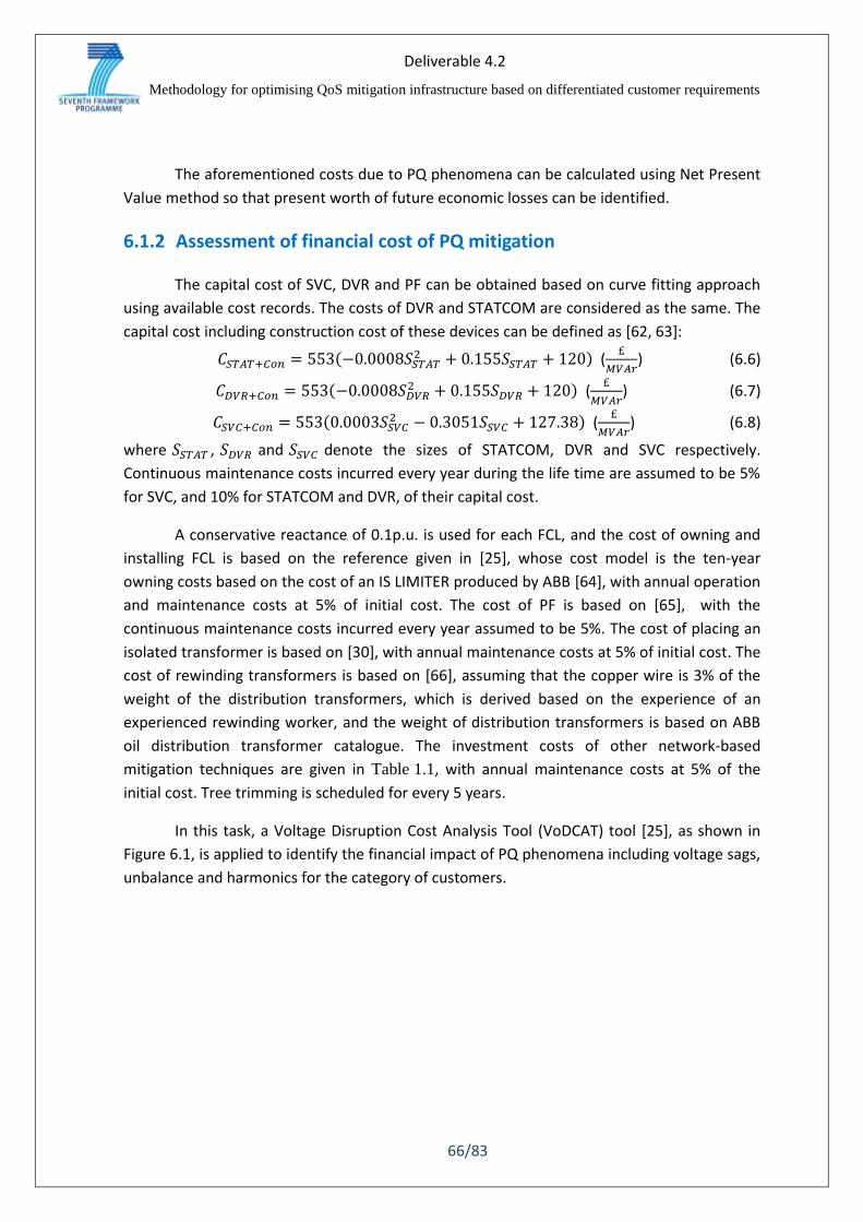
where 𝑆𝑆𝑇𝐴𝑇 , 𝑆𝐷𝑉𝑅 and 𝑆𝑆𝑉𝐶 denote the sizes of STATCOM, DVR and SVC respectively.

Continuous maintenance costs incurred every year during the life time are assumed to be 5%

for SVC, and 10% for STATCOM and DVR, of their capital cost.

A conservative reactance of 0.1p.u. is used for each FCL, and the cost of owning and

installing FCL is based on the reference given in [25], whose cost model is the ten-year

owning costs based on the cost of an IS LIMITER produced by ABB [64], with annual operation

and maintenance costs at 5% of initial cost. The cost of PF is based on [65], with the

continuous maintenance costs incurred every year assumed to be 5%. The cost of placing an

isolated transformer is based on [30], with annual maintenance costs at 5% of initial cost. The

cost of rewinding transformers is based on [66], assuming that the copper wire is 3% of the

weight of the distribution transformers, which is derived based on the experience of an

experienced rewinding worker, and the weight of distribution transformers is based on ABB

oil distribution transformer catalogue. The investment costs of other network-based

mitigation techniques are given in Table 1.1, with annual maintenance costs at 5% of the

initial cost. Tree trimming is scheduled for every 5 years.

In this task, a Voltage Disruption Cost Analysis Tool (VoDCAT) tool [25], as shown in

Figure 6.1, is applied to identify the financial impact of PQ phenomena including voltage sags,

unbalance and harmonics for the category of customers.

Deliverable 4.2


67/83

Figure 6.1: Layout of VoDCAT tool [25]

Table 6.1 shows the details of customers and their processes for which calculation of

customer customized financial loss is performed. A customer process model is built for each

customer based on their grouping. Sensitive equipment is identified based on the process

types and industry. Number of sub processes, connected power supply phase for equipment,

level of sensitivity, process dependency, process immunity time, process restart time, and

process cost factor were selected randomly from reasonable set of possible values. The

detailed inputs selected for evaluated customers can refer to reference [23]. Financial

analysis of sag for each customer type is performed using VoDCAT software. This software

first evaluates a customer damage function based on the customer business type identified

by NACE code. This evaluation is by using customer survey information on financial loss due

to power supply interruption updated into the tool database. Result of this evaluation is the

customer damage function for total process interruption caused due to sags. The tool then

calculates total financial losses for the customer sag profile which is given as input. Customer

process model, equipment sensitivity model and the customer damage function is used to

calculate the customized customer loss per year for the given sag profile. Using the Net

Present Value method mentioned above the losses can be estimated for the study period of

40 years. NPV of losses were normalized based on the peak KW demand of customer for

comparison. Table 6.2 [25], provides the sensitivity of each customer’s process to sags. It can

be seen that customer process with high sag sensitivity has more sensitive equipment and

dependent processes.

Table 6.1: Details of processes for different customers[25]

Cus PQ class. Sensitive equipment Sub

Process

Process dependency Matrix

A Sensitive PLC, ASD 1,2,3,4 1111,1101,1010,0111

B Essential PLC, ASD 1,2,3,4 1111,1101,0010,0111

C Essential PLC, ASD, Contactor 1,2,3,4 1111,1101,0010,1001

D Important PC, ASD 1,2,3,4 110,110,001

Deliverable 4.2


68/83

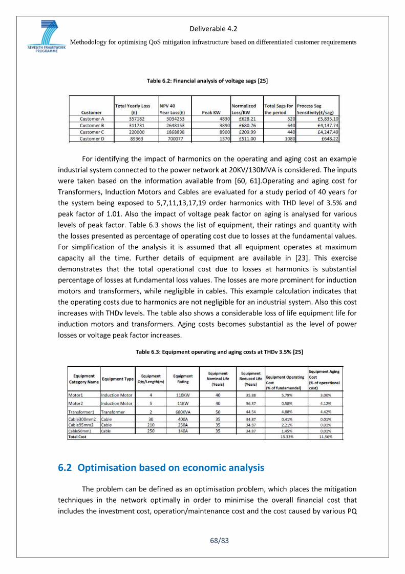
Table 6.2: Financial analysis of voltage sags [25]

For identifying the impact of harmonics on the operating and aging cost an example

industrial system connected to the power network at 20KV/130MVA is considered. The inputs

were taken based on the information available from [60, 61].Operating and aging cost for

Transformers, Induction Motors and Cables are evaluated for a study period of 40 years for

the system being exposed to 5,7,11,13,17,19 order harmonics with THD level of 3.5% and

peak factor of 1.01. Also the impact of voltage peak factor on aging is analysed for various

levels of peak factor. Table 6.3 shows the list of equipment, their ratings and quantity with

the losses presented as percentage of operating cost due to losses at the fundamental values.

For simplification of the analysis it is assumed that all equipment operates at maximum

capacity all the time. Further details of equipment are available in [23]. This exercise

demonstrates that the total operational cost due to losses at harmonics is substantial

percentage of losses at fundamental loss values. The losses are more prominent for induction

motors and transformers, while negligible in cables. This example calculation indicates that

the operating costs due to harmonics are not negligible for an industrial system. Also this cost

increases with THDv levels. The table also shows a considerable loss of life equipment life for

induction motors and transformers. Aging costs becomes substantial as the level of power

losses or voltage peak factor increases.

Table 6.3: Equipment operating and aging costs at THDv 3.5% [25]

6.2 Optimisation based on economic analysis

The problem can be defined as an optimisation problem, which places the mitigation

techniques in the network optimally in order to minimise the overall financial cost that

includes the investment cost, operation/maintenance cost and the cost caused by various PQ

Deliverable 4.2


69/83

phenomena, and to maximise the benefits as a result of the application of mitigation

techniques. Simultaneously, in planning PQ mitigation, the provision of differentiated PQ

levels should be facilitated among zones of the network based on customers’ requirement.

The provision of differentiated PQ levels is considered as the technical requirement, and

treated as a constraint to be imposed in the optimisation process. In the study, it is included

in the objective function using the approach of Lagrangian relaxation. The present value of

annual operation/maintenance cost and cost due to various PQ phenomena during the entire

life span of the deployed solution is calculated using NPV method. The overall objective

function (F) to be minimised in the optimisation problem is defined as:

𝐹 = 𝐶𝑚𝑖𝑡𝑖𝑔𝑎𝑡𝑖𝑜𝑛 − 𝐶𝑏𝑒𝑛𝑒𝑓𝑖𝑡 + 𝛽 × 𝑃𝑄𝐺𝐼UBPI (6.9)

𝐶𝑚𝑖𝑡𝑖𝑔𝑎𝑖𝑡𝑜𝑛 = 𝐶𝐼𝐶𝐼 +∑ (𝐶𝐴𝑛𝑛𝑂𝑝𝑒𝑀𝑎𝑖

𝑡 )×(1+𝑒)𝑡𝑛𝑡=0

((1+𝑟)(1+𝑖))𝑡 (6.10)

𝐶𝑏𝑒𝑛𝑒𝑓𝑖𝑡 =∑ (𝐶𝑃𝑄

1𝑡 −𝐶𝑃𝑄2𝑡 )×(1+𝑒)𝑡𝑛

𝑡=0

((1+𝑟)(1+𝑖))𝑡 (6.11)

where 𝐶𝑃𝑄1𝑡 and 𝐶𝑃𝑄

2𝑡 denotes the cost of PQ phenomena without and with mitigation at the

beginning of the time period respectively. To avoid confusion, all cost variables in (6.9)-(6.11)

are expressed as positive values (£). It can be seen that the smaller 𝐶𝑚𝑖𝑡𝑖𝑔𝑎𝑡𝑖𝑜𝑛 is, less

investment cost is required. The financial benefit of placing the mitigation techniques,

denoted as 𝐶𝑏𝑒𝑛𝑒𝑓𝑖𝑡, can be calculated by (𝐶𝑃𝑄1𝑡 − 𝐶𝑃𝑄

2𝑡 ). In (6.9), negative sign is applied to

𝐶𝑏𝑒𝑛𝑒𝑓𝑖𝑡 so that the optimisation procedure will attempt to maximise the benefit.

(𝐶𝑚𝑖𝑡𝑖𝑔𝑎𝑡𝑖𝑜𝑛 − 𝐶𝑏𝑒𝑛𝑒𝑓𝑖𝑡) < 0 suggests that the subsequent financial benefits resulting from

the application of mitigation techniques will cover the initial capital investment and

maintenance cost, and placing the selected mitigation scheme is beneficial in the long run. In

(6.9), 𝛽 is a Lagrange multiplier which imposes the penalty to the selected mitigation scheme

if the technical constraints are violated.

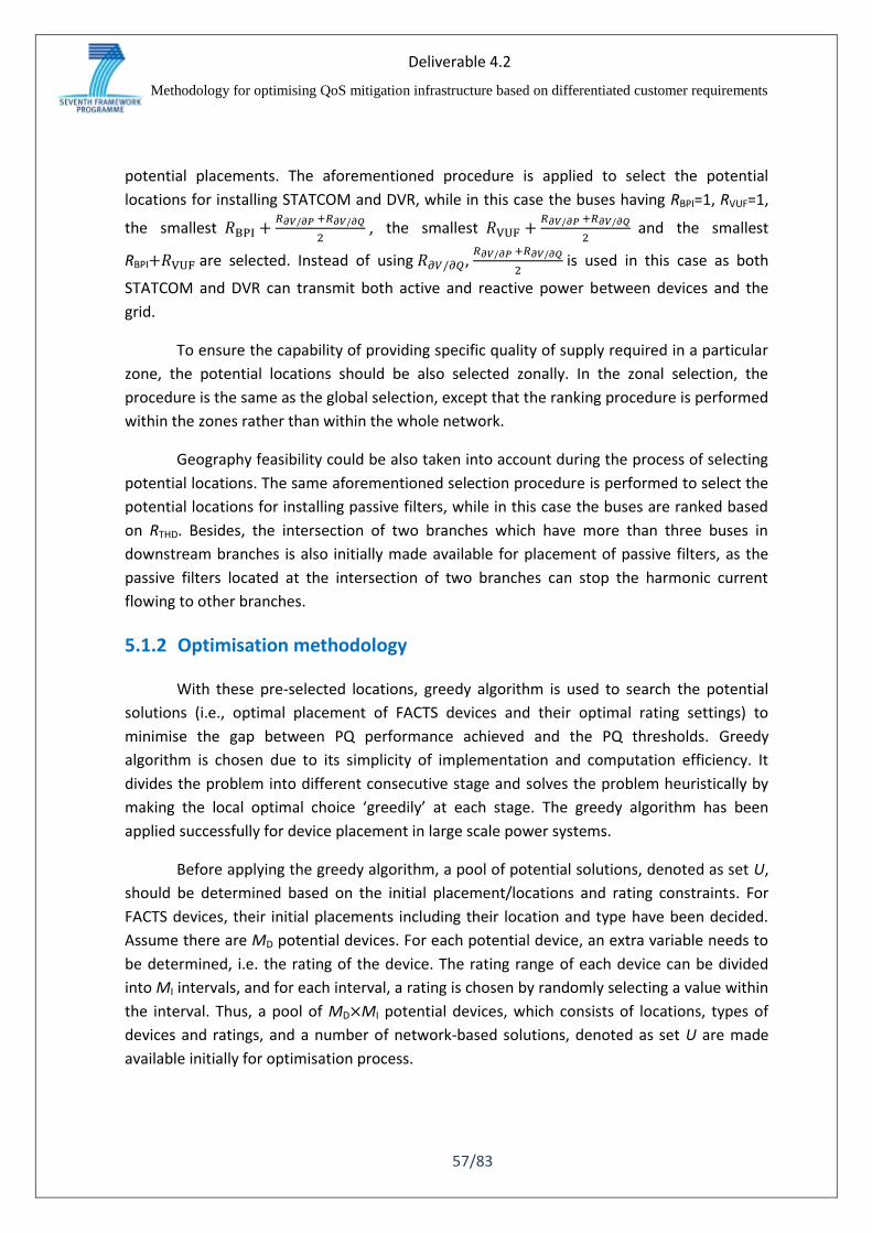
6.3 Simulation results

To present the impact of Lagrange multiplier 𝛽 in (6.9) on the final mitigation scheme,

𝛽 is set to 1E+8 and 1E+3 respectively in the simulation. The convergence curves of various

components in (6.9), including F, (𝐶𝑚𝑖𝑡𝑖𝑔𝑎𝑡𝑖𝑜𝑛 − 𝐶𝑏𝑒𝑛𝑒𝑓𝑖𝑡), 𝑃𝑄𝐺𝐼UBPI , 𝐶𝑚𝑖𝑡𝑖𝑔𝑎𝑡𝑖𝑜𝑛 , and 𝐶𝑃𝑄

which denotes the NPV of 𝐶𝑃𝑄2𝑡 , are presented in Figure 6.2. Without mitigation, only the

Lagrange component, i.e., the technical constraints of (UBPI-UBPITH), contributes to the

objective evaluation. At the leftmost points in Figure 6.2 (a), F=2.41E9 when 𝛽 = 1E8, and

F=2.41E4 when 𝛽 = 1E3. For both settings of 𝛽, the objective value F is reduced significantly

after one technique is applied to the grid. When the number of mitigation techniques>5, F

tends to converge steadily, though its improvement is not as significant as that when

mitigation techniques<5. When 10 mitigation techniques are applied, the objective value F

Deliverable 4.2


70/83

obtained with 𝛽 = 1E3 is smaller than that obtained when 𝛽 = 1E8 by 6.86E5. As seen from

(6.9), F is composed of (𝐶𝑚𝑖𝑡𝑖𝑔𝑎𝑡𝑖𝑜𝑛 − 𝐶𝑏𝑒𝑛𝑒𝑓𝑖𝑡) and 𝛽 × 𝑃𝑄𝐺𝐼UBPI. The two components are

presented in Figure 6.2 (b) and (c) respectively. Without any mitigation activity, both

𝐶𝑚𝑖𝑡𝑖𝑔𝑎𝑡𝑖𝑜𝑛 and 𝐶𝑏𝑒𝑛𝑒𝑓𝑖𝑡 are zero. Thus it can be seen from Figure 6.2 (b) that (𝐶𝑚𝑖𝑡𝑖𝑔𝑎𝑡𝑖𝑜𝑛 −

𝐶𝑏𝑒𝑛𝑒𝑓𝑖𝑡) = 0 when the number of techniques applied is zero. Afterwards, the obtained

(𝐶𝑚𝑖𝑡𝑖𝑔𝑎𝑡𝑖𝑜𝑛 − 𝐶𝑏𝑒𝑛𝑒𝑓𝑖𝑡) is smaller than zero constantly, which suggests that the financial

benefits resulting from the application of mitigation techniques at the network level will

cover the initial capital investment and maintenance cost. In Figure 6.2 (b), for the whole

convergence curves except for the leftmost points, (𝐶𝑚𝑖𝑡𝑖𝑔𝑎𝑡𝑖𝑜𝑛 − 𝐶𝑏𝑒𝑛𝑒𝑓𝑖𝑡) obtained when

𝛽 = 1E3 is always slightly smaller than that obtained when 𝛽 = 1E8; however, in Figure 6.2

(c), 𝑃𝑄𝐺𝐼UBPI obtained with 𝛽 = 1E3 is always slightly larger than that obtained when

𝛽 = 1E8. It can be seen that when 𝛽 is set to a larger number, i.e., 𝛽 = 1E8 in this case, the

optimisation will favour the mitigation schemes which are able to meet the technical

constraints well especially at the early stage of the optimisation process, compared to the

case of setting 𝛽 to a small number. Otherwise, the financial cost is the main reference for

the optimisation algorithm to select the mitigation solution. The costs of PQ phenomena and

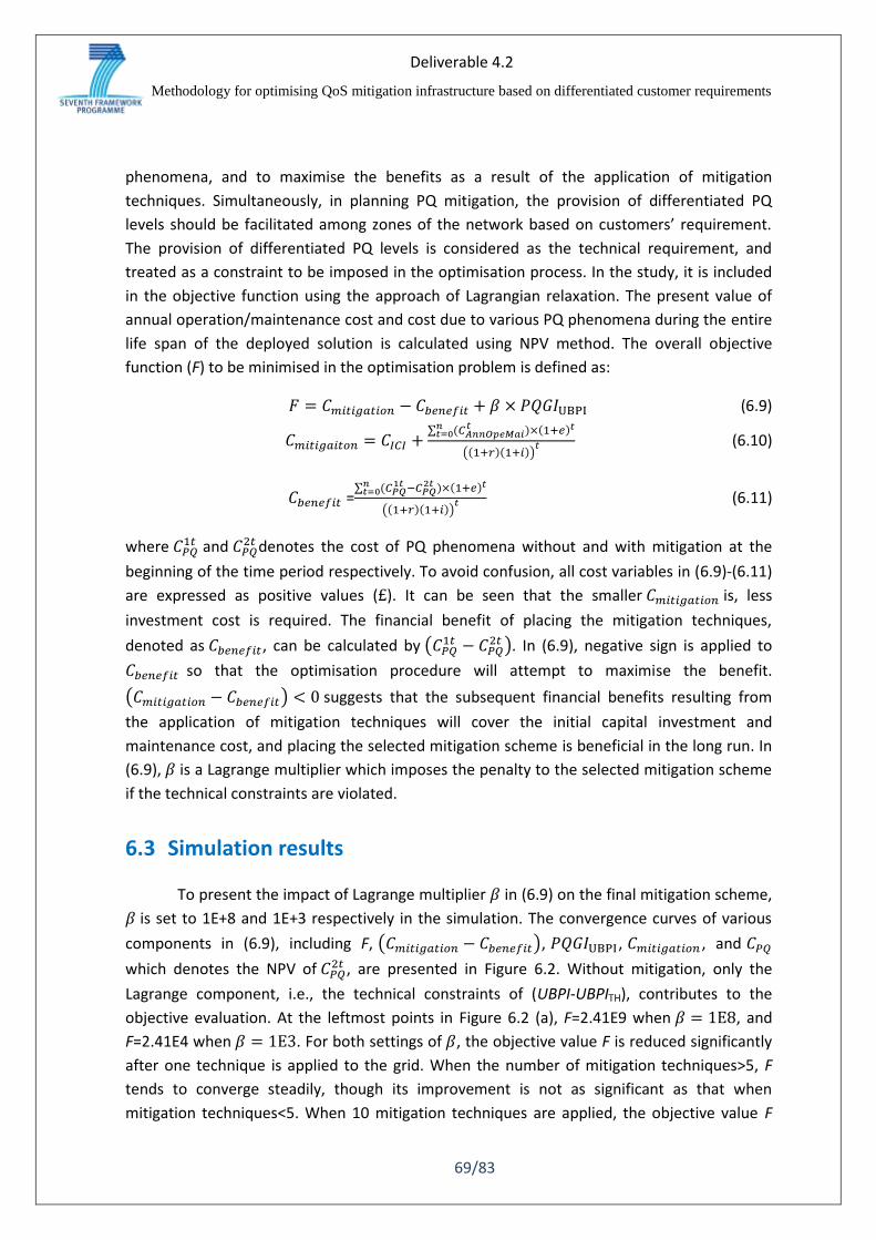
PQ mitigation are also presented in Figure 6.2 (d) and (e) respectively, and it can be seen that

𝐶𝑃𝑄 follows the same convergence trends as presented in Figure 6.2 (b). It can be concluded

that with a large 𝛽, the technical PQ requirements (minimizing the violation of set thresholds

for considered PQ phenomena) have more influence on the selection of the final solution

compared to the case of using small 𝛽 which places more influence on final cost of the

solution, i.e., payback period.

(a) F

(b) 𝐶𝑚𝑖𝑡𝑖𝑔𝑎𝑡𝑖𝑜𝑛 − 𝐶𝑏𝑒𝑛𝑒𝑓𝑖𝑡 (c) 𝑃𝑄𝐺𝐼UBPI

0 5 10-0.5

0

0.5

1

1.5

2

2.5x 10

9

No. of techs

F

0 5 10-8

-6

-4

-2

0

x 107

No. of techs

F

5 10-7.5

-7

x 107

=1E8

5 10-7.5

-7

x 107

=1E3

0 5 10-8

-6

-4

-2

0x 10

7

No. of techs

Cm

itig

atio

n-C

be

ne

fit

=1E8

=1E3

0 5 10

0

10

20

No. of techs

PQ

GI U

BP

I

=1E8

=1E3

Deliverable 4.2


71/83

(d) 𝐶𝑃𝑄 (e) 𝐶𝑚𝑖𝑡𝑖𝑔𝑎𝑡𝑖𝑜𝑛

Figure 6.2: Convergence curves of various components against the number of mitigation techniques applied

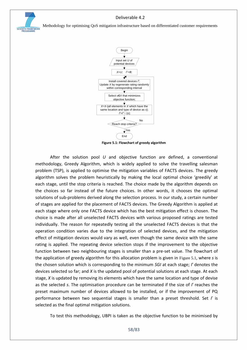
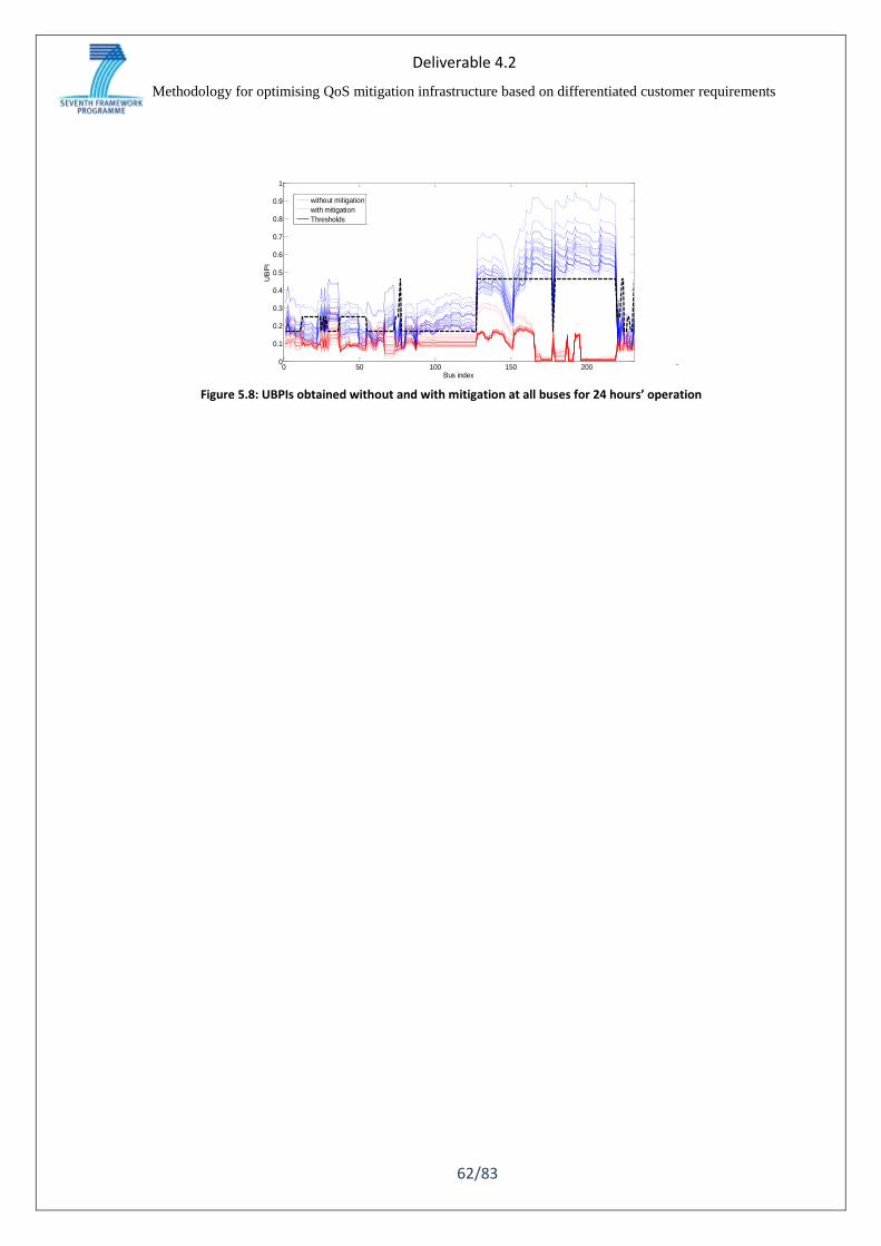
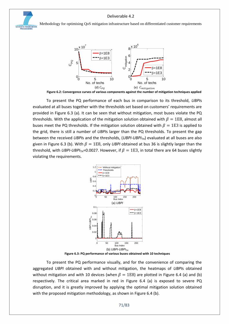
To present the PQ performance of each bus in comparison to its threshold, UBPIs

evaluated at all buses together with the thresholds set based on customers’ requirements are

provided in Figure 6.3 (a). It can be seen that without mitigation, most buses violate the PQ

thresholds. With the application of the mitigation solution obtained with 𝛽 = 1E8, almost all

buses meet the PQ thresholds. If the mitigation solution obtained with 𝛽 = 1E3 is applied to

the grid, there is still a number of UBPIs larger than the PQ thresholds. To present the gap

between the received UBPIs and the thresholds, (UBPI-UBPITH) evaluated at all buses are also

given in Figure 6.3 (b). With 𝛽 = 1E8, only UBPI obtained at bus 36 is slightly larger than the

threshold, with UBPI-UBPITH=0.0027. However, if 𝛽 = 1E3, in total there are 64 buses slightly

violating the requirements.

(a) UBPI

(b) UBPI-UBPITH

Figure 6.3: PQ performance of various buses obtained with 10 techniques

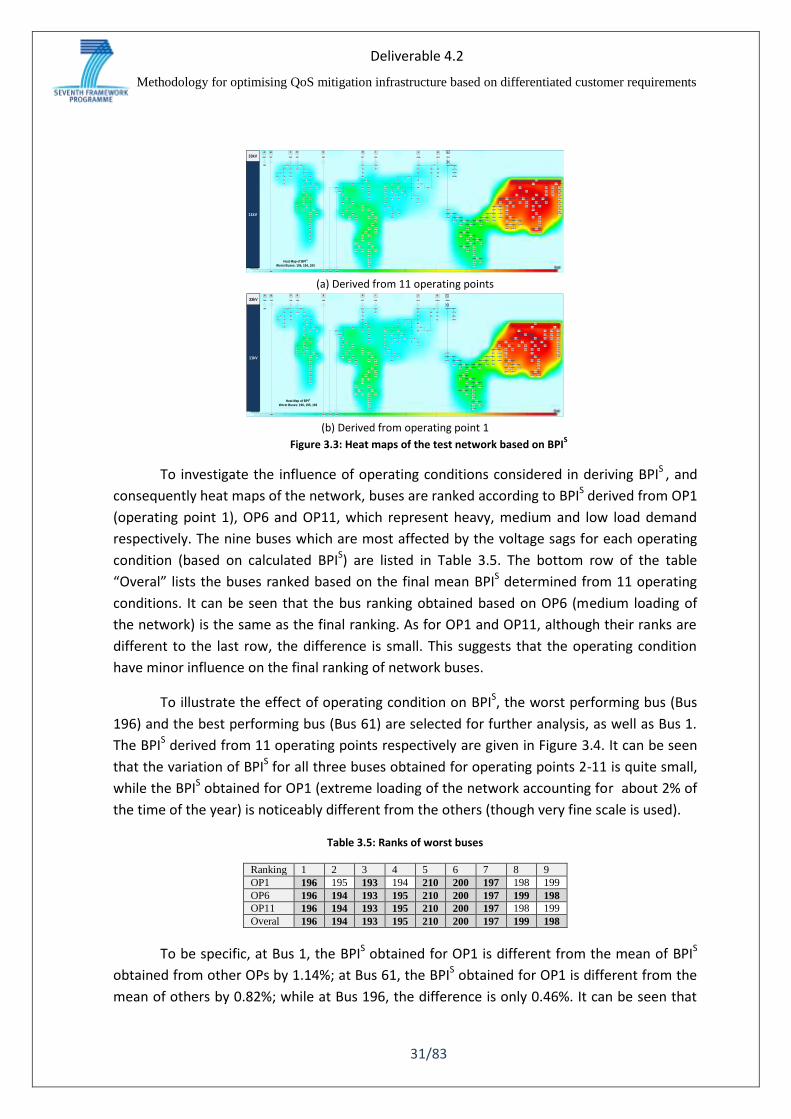
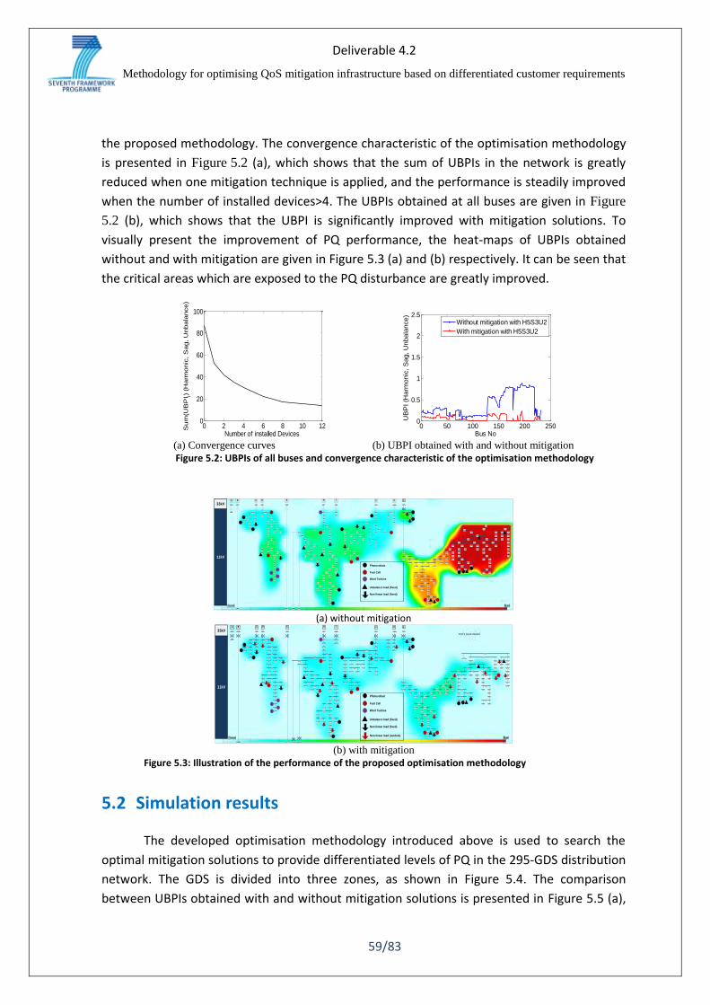
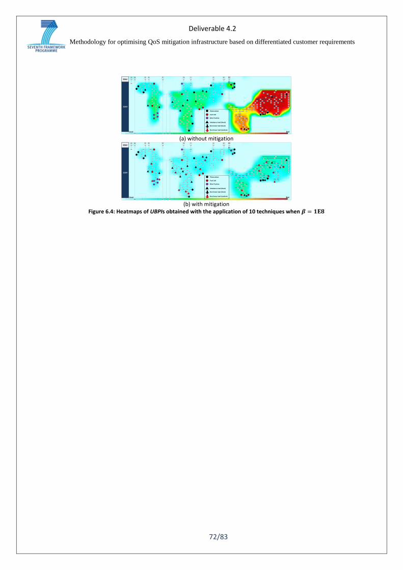
To present the PQ performance visually, and for the convenience of comparing the

aggregated UBPI obtained with and without mitigation, the heatmaps of UBPIs obtained

without mitigation and with 10 devices (when 𝛽 = 1E8) are plotted in Figure 6.4 (a) and (b)

respectively. The critical area marked in red in Figure 6.4 (a) is exposed to severe PQ

disruption, and it is greatly improved by applying the optimal mitigation solution obtained

with the proposed mitigation methodology, as shown in Figure 6.4 (b).

0 5 100

5

10x 10

7

No. of techs

CP

Q

=1E8

=1E3

0 5 100

2

4

6

8x 10

6

No. of techs

Cm

itig

atio

n

=1E8

=1E3

0 50 100 150 2000

0.2

0.4

0.6

0.8

1

1.2

Bus Index

UB

PI

Without mitigation

Thresholds

=1E8

=1E3

0 50 100 150 200

0

0.02

0.04

0.06

0.08

0.1

Bus Index

UB

PI-

UB

PI T

H

=1E8

=1E3

Deliverable 4.2


72/83

149

147

154

155

150 153 156

148 146

145

141

143

142

144

140

139

129

130 133

131

135

137 136

138

134

157

161

158

186

184

132

160

165

162

163

164

166

167

168169

170

180

181

182 183

185

187

188

189

190 191

192

193

194

197

198

200 199

201

202

203 204

205

206

207

208209

151

152

224

232

77

159

225

215

216

211

212210

213

214

217

218 171

219

220

172

173

174

175

176

177

178

265

195

196

L

24

46

17

28

16

14

12

26

21 19

23

223 22

18

15

54

52

53

230

50

75

228

74

229

20221

51 76

13

268

87

48 47

49222

43

42

41

40

39

38

37

269

231

78

79

80

81

85

88

290

82

83

84

291

91

92

93

95

94

96

97 98

101 99

100

102

103 104

105

106 107

108

109

110

111

112

113

114 115

116

121

122

123124

125

126

127

128

117

118

119 120

86

11

10

8

9

7

6

5

4

55

1 65

64

66 63

57

226 227

58

62

60

59

61

2

3

72

70

179

25

27

29

30

32

31 33

3435

36

7168

67 69

73

89

45

44

266267

289

238

288

269

287 285286

56

BA C D E H I J K

26426326033kV

11kV

H2 O2


Photovoltaic

Fuel Cell

Wind Turbine


Non-linear load (random)


149

147

154

155

150 153 156

148 146

145

141

143

142

144

140

139

129

130 133

131

135

137 136

138

134

157

161

158

186

184

132

160

165

162

163

164

166

167

168169

170

180

181

182 183

185

187

188

189

190 191

192

193

194

197

198

200 199

201

202

203 204

205

206

207

208209

151

152

224

232

77

159

225

215

216

211

212210

213

214

217

218 171

219

220

172

173

174

175

176

177

178

265

195

196

L

24

46

17

28

16

14

12

26

21 19

23

223 22

18

15

54

52

53

230

50

75

228

74

229

20221

51 76

13

268

87

48 47

49222

43

42

41

40

39

38

37

269

231

78

79

80

81

85

88

290

82

83

84

291

91

92

93

95

94

96

97 98

101 99

100

102

103 104

105

106 107

108

109

110

111

112

113

114 115

116

121

122

123124

125

126

127

128

117

118

119 120

86

11

10

8

9

7

6

5

4

55

1 65

64

66 63

57

226 227

58

62

60

59

61

2

3

72

70

179

25

27

29

30

32

31 33

3435

36

7168

67 69

73

89

45

44

266267

289

238

288

269

287 285286

56

BA C D E H I J K

26426326033kV

11kV

H2 O2


Photovoltaic

Fuel Cell

Wind Turbine


Non-linear load (random) (b) with mitigation

Figure 6.4: Heatmaps of UBPIs obtained with the application of 10 techniques when 𝜷 = 𝟏𝐄𝟖

Deliverable 4.2


73/83

6.4 Economically incentivised solution to mitigate LV network

harmonics

Based on the network modelling method developed in section 3.5 and the mitigation

methods analysed in section 4.3, a framework to incentivise customers to use switched-mode

ac-dc converters to offer harmonic compensation is proposed. Compensation is favoured

over reduction of emissions because incentives are based on spatial factors. In order to allow

fair access to the grid, it would not be appropriate to penalise users who connect line

frequency diode bridge converter interfaced devices because of where they are in the

network.

The ability to provide and the costs of compensation are dependent on technology

development. Therefore it is proposed to develop economic incentives designed to help

stimulate this development. In order to do that, a fair value is calculated for the benefit

gained by the system operator from these solutions.

The costs of the filter considered in section 4.3.1 is estimated to be 935 € [65] per

phase. The value attributable to system losses is calculated using the following method. The

temporal variation of losses is based on standard domestic load curves, such as shown in

Figure 6.5 [53].

Figure 6.5: Representative load profile for January in Germany.

The proportion of harmonics in this load curve is assumed to be constant. The load

curves cover all months of the year and therefore an average annual loss can be calculated. In

addition, the annual monetary savings from the filters and from the harmonic reduction or

distributed compensation at each node can be calculated.

Deliverable 4.2


74/83

The calculation assumes an energy price of 40 €/MWh [67]. Compensation of the 3rd,

5th and 7th harmonics are considered (these cause the large majority of voltage THD and

system losses). The results are normalised to a compensated current of 1 A in each phase. To

place this in context, a 100 W device with line frequency diode bridge converter, fed by a

pure 50 Hz sine wave, operating at full power, draws 2.6 A, 1.8 A and 0.9 A at the 3rd, 5th and

7th harmonics respectively. The results are plotted showing the effect on system losses

against distance from the main bus at which compensation is provided are shown in Figure

6.6. The effect on the worst case of voltage THD in the system (node R18) for compensation

at each node is shown in

Table 6.4.

Figure 6.6: Reduction of system losses by harmonic compensation of 1 A in each phase against the distance from the main bus of the node at which compensation takes place.

Table 6.4: Reduction of voltage THD in phase b at node R18 by compensation of 1 A of harmonic current in each phase for each node.

Harmonic Order

Compensated Node

R1 R11 R15 R16 R17 R18

3 0% 0.0156% 0.0169% 0.0358% 0.0605% 0.0554%

5 0% 0.0165% 0.0219% 0.0386% 0.0622% 0.0561%

7 0% 0.0065% 0.0085% 0.0151% 0.0246% 0.0225%

The value of the THD reduction from the compensation can then be calculated:

𝐶𝑜𝑚𝑝𝑒𝑛𝑠𝑎𝑡𝑖𝑜𝑛 𝑉𝑎𝑙𝑢𝑒 𝑝𝑒𝑟 𝑎𝑚𝑝 =𝐹𝑖𝑙𝑡𝑒𝑟 𝐶𝑜𝑠𝑡𝑠× 𝑇𝐻𝐷 𝑟𝑒𝑑𝑢𝑐𝑡𝑖𝑜𝑛 𝑝𝑒𝑟 𝑎𝑚𝑝

𝑈𝑛𝑚𝑖𝑡𝑖𝑔𝑎𝑡𝑒𝑑 𝑇𝐻𝐷−𝑃𝑒𝑟𝑚𝑖𝑡𝑡𝑒𝑑 𝑇𝐻𝐷 (6.12)

Deliverable 4.2


75/83

From

Table 6.4, it can be seen that the most effective way to reduce THD at node R18 is by

compensation of the 5th harmonic at node R17. As an example, based on filter costs of 3

times 935 € (1 filter in each phase) and an unmitigated voltage THD at node R18 of 5.15%

(Table 3.9), the value of compensation at node R17 for the 5th harmonic is 1163 € per amp

(provided to all phases). This compensation would only be called upon when required but

would need to be made available at all times over the estimated lifetime of a filter.

For both voltage THD and loss reduction, it should be noted that these values are

based on a small initial level of compensation. Only a finite level of harmonic compensation is

required to mitigate voltage THD and loss reduction is not linear with current reduction. In

the event that more compensation became available from distributed energy resources than

required, market forces would ultimately dictate the value of incentives.

Deliverable 4.2


76/83

7 Conclusions

The report presents the concept of provision of differentiated quality of electricity

supply based on customers’ requirements in distribution networks. To fulfil this concept, five

new gap indices are introduced to reflect the satisfaction of the received PQ performance

compared to the thresholds which are set based on customers’ requirement regarding the

performance of individual PQ phenomenon or the aggregated PQ performance.

A range of PQ mitigating solutions was investigated to insure cost-effective

management of PQ in the network. FACTS devices including SVC, STATCOM and DVR were

investigated for PQ mitigation. Besides, network/plant based mitigation techniques were also

tested as the potential solutions to the PQ problems at hand. The effectiveness of these

mitigation techniques were evaluated using the selected severity indices and validated in

295-bus GDS.

Using the new gap indices as objective functions, an optimisation-based mitigation

strategy was proposed to carry out the strategic placement of potential FACTS devices based

on the analysis of PQ performance and sensitivity analysis. In this methodology, greedy

algorithm is applied to search the optimal mitigation scheme in order to enable the provision

of differentiated PQ levels. The feasibility of the proposed mitigation methodology was

demonstrated in a large scale generic distribution network. The pros and cons of using the

proposed indices as the optimisation objective functions are analysed in the report.

This report also presents an optimisation-based PQ mitigation methodology which

accounts for the comprehensive analysis of the financial losses due to critical PQ phenomena

as a result of industrial process trips, equipment aging issues and power losses, etc. This

report introduces the methodologies of assessing the financial investment of various

mitigation techniques (including network-based and FACTS devices-based mitigation

solutions) during the entire life span of the deployed solution. The proposed mitigation

methodology facilitates the provision of differentiated levels of PQ supply as required by

customers in different zones, by integrating the technical requirements in the optimisation

process as constraints using the approach of Lagrangian relaxation. The proposed

methodology was tested in a large scale 295-bus generic distribution network taking into

account a number of uncertainty factors. The simulation results demonstrated that placing

the mitigation scheme obtained by the proposed methodology is beneficial in the long run, as

the financial benefits of applying the mitigation techniques are much larger than the initial

capital investment and maintenance cost of the PQ mitigation.

The developed modelling method for the LV network highlighted the need for

detailed analysis of cable performance and showed that accurate cable parameters are

essential in planning harmonic mitigation. Of the mitigation methods considered, it was

Deliverable 4.2


77/83

shown that harmonic compensation is an effective method and that meaningful economic

incentives are possible based on the value offered to the network.

Deliverable 4.2


78/83

References

[1] J. Y. Chan, J. V. Milanović, and A. Delahunty, "Risk-based assessment of financial losses due to voltage sag," IEEE Trans. Power Del., vol. 26, pp. 492-500, 2011.

[2] R. S. Thallam, "Power quality indices based on voltage sag energy values," in Proc. Power Quality Conf. Expo., Chicago, IL, 2001.

[3] M. H. J. Bollen, D. D. Sabin, and R. S. Thallam, "Voltage-sag indices - recent developments in IEEE P1564 task force," in Proc. IEEE PES Int. Symp. Quality and Security of Electric Power Delivery Systems (CIGRE), 2003, pp. 34-41.

[4] R. S. Thallam and G. T. Heydt, "Power acceptability and voltage sag indices in the three phase sense," in Proc. IEEE Power Eng. Soc. Summer Meeting, Seattle, WA, 2000, pp. 905-910.

[5] M. H. J. Bollen and I. Y. H. Gu, Signal Processing of Power Quality Disturbances. New York, NY, USA: IEEE Press, 2006.

[6] A. Robert and E. D. Jaeger, "Final Rep. round table on power quality at the interface T&D CIRED 2003," May. 14, 2003.

[7] M. H. J. Bollen and D. D. Sabin, "International coordination for voltage sag indices," in Proc. IEEE PES Transmission and Distribution Conference and Exhibition, 2006, pp. 229-234.

[8] J. Y. Chan and J. V. Milanović, "Severity indices for assessment of equipment sensitivity to voltage sags and short interruptions," in Proc. IEEE Power Eng. Soc. Gneral Meeting, Tampa, FL, 2007, pp. 1-7.

[9] J. Y. Chan, J. V. Milanović, and A. Delahunty, "Generic failure-risk assessment of industrial processes due to voltage sags," IEEE Trans. Power Del., vol. 24, pp. 2405-2414, 2009.

[10] A. M. Dan, "Introducing a voltage dip severity index (a proposal)," in Proc. Int. Conf. on Harmonics Quality of Power, 2010, pp. 1-5.

[11] C. N. Lu and C. C. Shen, "A voltage sag index considering compatibility between equipment and supply," IEEE Trans. Power Del., vol. 22, pp. 996-1002, 2007.

[12] C. N. Lu and C. C. Shen, "Voltage sag immunity factor considering severity and duration," in Proc. IEEE Power Eng. Soc. Gneral Meeting, 2004, pp. 626-630

[13] C. N. Lu and C. C. Shen, "Estimation of sensitive equipment disruptions due to voltage sags," IEEE Trans. Power Del., vol. 22, pp. 1132-1137, 2007.

[14] F. B. Costa and J. Driesen, "Assessment of voltage sag indices based on scaling and wavelet coefficient energy analysis," IEEE Trans. Power Del., vol. 28, pp. 336-346, 2013.

[15] G. J. Wakileh, Power Systems Harmonics: Fundamentals, Analysis and Filter Design. New York: Springer, 2001.

[16] Spec. Semicon. Process, Equipment Voltage Sag Immunity, SEMI-F47-0706. Available: www. Semi.org.

[17] G. Tsagarakis, A. J. Collin, and A. E. Kiprakis, "Modelling the electrical loads of UK residential energy users," in Proc. 47th Int. Universities Power Eng. Conf., London, 2012, pp. 1-6.

[18] "Technology roadmap: Electric and plug-in hybrid electric vehicles," International Energy Agency, 2011.

[19] "Technology roadmap: solar photovoltaic energy," International Energy Agency, 2010. [20] N. C. Woolley and J. V. Milanović, "Statistical estimation of the source and level of voltage

unbalance in distribution networks," IEEE Trans. Power Del., vol. 27, pp. 1450-1460, 2012. [21] A. Robert and J. Marquet, "“Assessing Voltage Quality with relation to Harmonics, Flicker

and Unbalance,”" WG 36.05, Paper 36-203, CIGRE 92.

Deliverable 4.2


79/83

[22] W. H. Kersting, "Causes and effects of unbalanced voltages serving an induction motor," in Rural Electric Power Conference, 2000, 2000, pp. B3/1-B3/8.

[23] J. Thomas, "Development of methodology for online provision of differentiated quality of electricity supply," MSc. Electrical Power Systems, Fac. of Eng. and Phys. Sciences, The University of Manchester, 2012.

[24] T. G. More, P. R. Asabe, and C. S., "Power quality issues and It’s mitigation techniques," Int. J. of Eng. Research and App., vol. 4, pp. 170-177, 2014.

[25] J. Y. Chan, "Framework for assessment of economic feasibility of voltage sag mitigation solutions," Ph.D., Ph.D. dissertation, Dep. Electr. And Electro. Eng., University of Manchester, Manchester, U.K., 2010.

[26] E. Cinieri and F. Muzi, "Lightning induced overvoltages, improvement in quality of service in MV distribution lines by addition of shield wires," IEEE Trans Power Del. , vol. 11, pp. 361-372, 1996.

[27] T. A. Short, Electric Power Distribution Handbook. New York: CRC Press, 2004. [28] W. A. Chisholm, "Outline of guide for application of transmission line surge arresters 42 to

765 kV," Electric Power Reserch Institue, 1012313, 2006. [29] J. Sanders and K. Newman, "Polymer arresters as an alternative to shield wire," Hubbell

Power Systems Inc., EU1413-H, 1992. [30] T. C. Sekar and B. J. Rabi, "A review and study of harmonic mitigation techniques," in Proc.

Int. Emer. Trends in Elec. Eng. and Ener. Manag., Chennai, 2012. [31] H. Masdi, N. Mariun, S. Mahmud, A. Mohamed, and S. Yusuf, "Design of a prototype D-

STATCOM for voltage sag mitigation," in Proc. National Power and Energy Conf., Kuala Lumpur, Malaysia, 2004, pp. 61-66.

[32] Y. Xiao, Y. H. Song, C. C. Liu, and Y. Z. Sun, "Available transfer capability enhancement using FACTS devices," IEEE Trans. Power Syst., vol. 18, pp. 305-312, 2003.

[33] E. Ghahremani and I. Kamwa, "Optimal placement of multiple-type FACTS devices to maximize power system loadability using a generic graphical user interface," IEEE Trans. Power Syst., vol. 28, pp. 764-778, 2013.

[34] H. Hatami, F. Shahnia, A. Pashaei, and S. H. Hosseini, "Investigation on D-STATCOM and DVR operation for voltage control in distribution networks with a new control strategy," in Proc. IEEE Lau. Power Tech., 2007, pp. 2207-2212.

[35] R. Asati and N. R. Kulkarni, "A review on the control strategies used for DSTATCOM and DVR," Int. J. of Elec., Electr. Comp. Eng., vol. 2, pp. 59-64, 2013.

[36] H. L. Liao, S. Abdelrahman, and J. V. Milanović, "Identification of weak areas of power network based on exposure to voltage sags — part I: development of sag severity index for single-event characterization," IEEE Trans. Power Del. (accepted), 2014.

[37] H. L. Liao, S. Abdelrahman, Y. Guo, and J. V. Milanović, "Identification of weak areas of power network based on exposure to voltage sags—Part II: assessment of network performance using sag severity index," IEEE Trans. Power Del. (accepted), 2014.

[38] L. G. Vargas and T. L. Saaty, Models, Methods, Concepts & Applications of the Analytic Hierarchy Process. New York: Springer Science and Business Media, 2012.

[39] R. Dugan, M. F. McGranaghan, S. Santoso, and H. W. Beaty, Electrical Power Systems Quality (2 Ed.). New York: McGraw-Hill, 2002.

[40] M. T. Aung and J. V. Milanović, "Stochastic prediction of voltage sags by considering the probability of the failure of the protection system," IEEE Trans Power Del., vol. 21, pp. 322-329, 2006.

Deliverable 4.2


80/83

[41] Z. Liu and J. V. Milanovic, "Probabilistic estimation of propagation of unbalance in Distribution Network with asymmetrical loads," in Proc. 8th Medi. Conf. on Power Gen., Tran., Distri. and Ene. Conver., 2012, pp. 1-6.

[42] S. Abdelrahman, H. Liao, J. Yu, and J. V. Milanović, "Probabilistic assessment of the impact of distributed generation and non-linear load on harmonic propagation in power systems," in Proc. 18th Pow. Syst. Com. Conf. , Wroclaw, Poland, 2014.

[43] CM SAF JRC EUROPEAN COMMISSION. Photovoltaic Geographical Information System - Interactive Maps [Online]. Available: http://re.jrc.ec.europa.eu/pvgis/apps4/pvest.php.

[44] "The Renewable Energy Review," Committee on Climate Change, 2011. [45] G. Olguin and M. H. J. Bollen, "Stochastic assessment of unbalanced voltage dips in large

transmission systems," in Proc. IEEE Bologna Power Tech 2003, p. 8 pp. Vol.4. [46] A. A. Groppelli and E. Nikbakht, Finance: Barrons Educational Series Inc, 2000. [47] C. A. Canesin, L. C. O. d. Oliveira, J. B. Souza, D. D. O. d. Lima, and R. P. Buratti, "A time-

domain harmonic power-flow analysis in electrical energy distribution networks, using Norton models for non-linear loading," in Proc. IEEE 16th Int. Con. on Harmonics and Quality of Power, Bucharest, 2014, pp. 778-782.

[48] E. Thunberg and L. Soder, "A Norton approach to distribution network modeling for harmonic studies," IEEE Trans. Power Deli., vol. 14, pp. 272–277, 1999.

[49] IEC 61000-3-2:2002, "Limits for Harmonic Current Emissions (Equipment Input Current up to and including 16A Per Phase)," ed, 2003.

[50] J. Arrillaga and N. R. Watson, Power System Harmonics (2nd Edition): Wiley, 2003. [51] T. B. Wood, D. E. Macpherson, D. Banham-Hall, and S. J. Finney, "Ripple current

propagation in bipole HVDC cables and applications to DC grids," IEEE Trans. Power Deli., vol. 29, pp. 926–933, 2014.

[52] K. Strunz etc., "Benchmark systems for network integration of renewable and distributed energy resources, Cigre Task Force C 6," 2009.

[53] EWE Netz GmbH, "Lastprofile 2014, available: https://www.ewe-netz.de/strom/1988.php," 2014.

[54] Y. Zhao, C. Wang, and J. Yan, "Analysis on Topology of DVR Used in Low-voltage Distribution Grid," Int. J. of Eng. Sci. and Research Tech., vol. 2, pp. 3630-3633, 2013.

[55] M. S. Munir and Y. W. Li, "Residential Distribution System Harmonic Compensation Using PV Interfacing Inverter," IEEE Trans. Smart Grid, vol. 4, pp. 816-827, 2013.

[56] M. Abinaya, N. Senthilnathan, and M. Sabarimuthu, "Harmonic Compensation as Ancillary Service in PV Inverter Based Residential Distribution System," in Proc. Int. Con. on Circuit, Power and Comp. Tech., Nagercoil, 2014, pp. 490-495.

[57] H. Geng, L. V. Qing, and G. Yeng, "Harmonic mitigation performance of the power inverter based DG in a AC microgrid," in Proc. IEEE 23rd Int. Symp. on Ind. Electron., Istanbul, 2014, pp. 2379-2384.

[58] J. G. Lglesias etc., "Economic framework for power quality, JWG CIGRE-CIRED C4.107," 2011.

[59] N. E. M. Association, "NEMA Standards Publication MG 1-1998 Motors and Generators," ed, 2002.

[60] P. Caramia, G. Carpinelli, P. Verde, G. Mazzanti, A. Cavallini, and G. C. Montanari, "An approach to life estimation of electrical plant components in the presence of harmonic distortion," in Proc. 9th Int. Conf. on Harm. and Quality of Power, 2000, pp. 887-892 vol.3.

[61] G. C. Montanari and L. Simoni, "Aging phenomenology and modeling," IEEE Trans. Elec. Insul., vol. 28, pp. 755-776, 1993.

Deliverable 4.2


81/83

[62] J. V. Milanović and Z. Yan, "Global minimization of financial losses due to voltage sags with FACTS based devices," IEEE Trans. on Power Del., vol. 25, pp. 298-306, 2010.

[63] Y. Zhang, "Techno-economic Assessment of Voltage Sag Performance and Mitigation," Ph.D., Ph.D. dissertation, Dep. Electr. And Electro. Eng., University of Manchester, Manchester, U.K., 2008.

[64] A. Cali, S. Conti, F. Santonoceto, and G. Tina, "Benefits assessment of fault current limiters in a refinery power plant: a case study," in Proc. Int. Conf. Power System Tech., 2000, pp. 1505-1510 vol.3.

[65] M. Ghiasi, V. Rashtchi, and S. H. Hoseini, "Optimum location and sizing of passive filters in distribution networks using genetic algorithm," in Proc. Int. Conf. on Emer. Tech., 2008, pp. 162-166.

[66] M. Mohan, "Amorphous-Core Transformer with Copper Winding Versus Aluminium Winding-A Comparative Study," ARPN Journal of Science and Technology, vol. 2, pp. 297-301, 2012.

[67] "Electricity Production and Spot-Prices in Germany 2014, available: https://www.ise.fraunhofer.de/de/downloads/pdf-files/data-nivc-/folien-electricity-spot-prices-and-production-data-in-germany-2014-engl.pdf," Fraunhofer Institute for Solar Energy System, 2014.

Deliverable 4.2


82/83

Appendix A: List of publications based on this report

Journal papers

[D1] H.L. Liao, S. Abdelrahman, Y. Guo, and J.V. Milanovic, "Identification of Weak Areas of Power

Network Based on Exposure to Voltage Sags -Part I: Development of Sag Severity Index for Single-

Event Characterization," accepted for publication in the IEEE Trans. Power Del., DOI:

10.1109/TPWRD.2014.2362965

[D2] H.L. Liao, S. Abdelrahman, Y. Guo, and J.V. Milanovic, "Identification of Weak Areas of

Network Based on Exposure to Voltage Sags -Part II: Assessment of Network Performance Using

Sag Severity Index," accepted for publication in the IEEE Trans. Power Del., DOI:

10.1109/TPWRD.2014.2362957

[D3] Z.Liu and J.V.Milanović, “Probabilistic estimation of voltage unbalance in mv

distribution networks with unbalanced load”, IEEE Transactions on Power Delivery, Vol.

30, No 2, 2015, pp. 693 – 703

[D4] Huilian Liao, Zhixuan Liu, J. V. Milanović, and Nick C. Woolley, “Optimisation

Framework for Development of Cost-effective Monitoring in Distribution Networks“,

accepted for publication in the IET Generation, Transmission and Distribution, GTD-2015-

0757

Conference papers

[D5] S. Abdelrahman, H.L. Liao, J. Yu and J.V. Milanović, "Probabilistic assessment of the impact of

distributed generation and non-linear load on harmonic propagation in power systems”, in Proc.

18th Power Systems Computation Conference (PSCC), Wroclaw, Poland, 2014.

[D6] S. Abdelrahman, H.L. Liao and J.V. Milanović, “The Effect of Temporal and Spatial Variation of

Harmonic Sources on Annual Harmonic Performance of Distribution Networks”, in Proc. 5th IEEE

PES Innovative Smart Grid Technologies Europe (ISGT), Istanbul, Turkey, 2014.

[D7] H.L. Liao, S. Abdelrahman and J.V. Milanović, “Provision of Differentiated Voltage Sag

Performance Using FACTS Devices”, in Proc. 23rd International Conference and Exhibition on

Electricity Distribution (CIRED 2015), France, June 2015.

Deliverable 4.2


83/83

[D8] H.L. Liao and J.V. Milanović, “Comparative Analysis of Different Voltage Sag

Characterisation Indices”, in Proc. 23rd International Conference and Exhibition on Electricity

Distribution (CIRED 2015), France, June 2015.

[D9] H.L. Liao, J. Saif and J.V. Milanović, “Provision of Differentiated Power Quality Using

Network Based Mitigating Solutions”, in Proc. 23rd International Conference and Exhibition

on Electricity Distribution (CIRED 2015), France, June 2015.

[D10] S. Abdelrahman, H.L. Liao and J.V. Milanović “Characterisation of Power Quality

Performance at Network Buses Using Unified Power Quality Index", in Proc. 23rd

International Conference and Exhibition on Electricity Distribution (CIRED 2015), France, June

2015.

[D11] S. Abdelrahman, H. Liao, T. Guo, Y. Guo and J.V. Milanovic “Global Assessment of Power

Quality Performance of Networks using the Analytic Hierarchy Process Model”, POWERTECH,

Netherlands, June 2015.

Submitted Journal papers

[D12] J. V. Milanović, Sami Abdelrahman and Huilian Liao, “Compound Index for Power

Quality Evaluation and Benchmarking“, submitted to the IEEE Transactions on Power

Delivery, TPWRD-00141-2015, (3/2/15;8/5/15;1/9/15)

[D13] Huilian Liao and J. V. Milanović, “Analysis of Propagation of Voltage Unbalance in

Distribution Networks with Distributed Generation “, submitted to the IEEE Transactions

on Power Delivery, TPWRD-01272-2015, (08/09/15)

[D14] Huilian Liao and J. V. Milanović, “Merits of Different FACTS Devices for Mitigation

of Power Quality Phenomena“, submitted to the IEEE Transactions on Power Delivery,

TPWRD-01382-2015, (08/10/15)

Date post:	11-May-2018
Category:	Documents
Upload:	votram
View:	217 times
Download:	1 times

Methodology for optimising QoS mitigation infrastructure ... · 5.2 Simulation results ... Figure...

Documents