QUANTITATIVE FINANCE RESEARCH CENTRE QUANTITATIVE F INANCE RESEARCH CENTRE QUANTITATIVE FINANCE RESEARCH CENTRE Research Paper 396 October 2018 Methods for Analytical Barrier Option Pricing with Multiple Exponential Time-Varying Boundaries Otto Konstandatos ISSN 1441-8010 www.qfrc.uts.edu.au
Transcript
QUANTITATIVE FINANCE RESEARCH CENTRE QUANTITATIVE F
INANCE RESEARCH CENTRE
QUANTITATIVE FINANCE RESEARCH CENTRE
Research Paper 396 October 2018
Methods for Analytical Barrier Option Pricing with Multiple Exponential Time-Varying Boundaries
Otto Konstandatos
ISSN 1441-8010 www.qfrc.uts.edu.au
Methods for Analytical Barrier Option Pricing with Multiple ExponentialTime-Varying Boundaries
Otto Konstandatos
Discipline of FinanceUniversity of Technology Sydney, NSW 2007, Australia
Abstract
We develop novel methods for efficient analytical solution of all types of partial time barrier options with both single
and double exponential and time varying boundaries, and specifically to treat forward-starting partial double barrier
options, which present the simplest non-trivial example of the multiple exponential time-varying barrier case. Our
methods reduce the pricing of all barrier options with time-varying boundaries to the pricing of a single European
option. We express our novel results solely in terms of European first and second order Gap options. We are motivated
by similar structures appearing in Structural Credit Risk models for firm default.
Keywords: Exotic Options, Method of Images, Partial Time Double Barrier Options, Window Double Barrier
Barrier options however have a wider significance than just for exotic options on equities. An important reason for
studying barrier option structures, and indeed a major motivation for this study, stems from the potential application
that barrier options have in structural credit risk models which use the value of a firm to determine time of firm default.
The first structural credit-risk model was Merton (1974), which extended the seminal Black and Scholes (1973) to
the value of the firm, modelled as a stochastic process driven by Geometric Brownian Motion. In this model default
occurs at the time of ‘debt servicing’ (corresponding to option expiry) if the firm’s asset value is insufficient to repay
outstanding debt. The default boundary is just the face value of the debt. However defaults can occur at any time.
An extension of the structural approach relevant here was undertaken in Black and Cox (1976). This work assumed
that default occurs as soon as the value of a firm’s assets drop below a certain threshold. Such thresholds have natural
interpretations as knock-out barriers on the firm’s value. Structural models of credit default therefore naturally share
features with equity options having knock-out barrier features.
The value of the outstanding debt triggering default, namely the ‘credit default barrier’ may naturally be considered
to be exponential and time-varying due to the time-value of money, rather than constant. Multiple exponential and
time-varying barrier levels may be interpreted as thresholds triggering rating upgrades, downgrades and default in the
manner of CreditMetrics (see Gupton et al. (1997))1.
Although we do not explicitly treat the problem of credit default modelling in this work due to its unique challenges,
we note that credit downgrade/default and credit upgrade scenarios naturally give rise to lower and upper exponential
and time-varying barrier levels for the value of a firm for which the current state of the art is Monte-Carlo simulation.
The application to credit risk scenarios is an important motivation for examining techniques for the efficient treatment
of barrier option structures with multiple exponential and time-varying lower and upper boundaries, of which the
partial-time late monitoring double barrier scenario is the simplest non-trivial case. The methodology we employ here
points a way to getting tractable solutions in a multi-barrier context when using proper Black-Scholes dynamics for
the firm value.
1.1. Background
In the classic Black-Scholes model, there is a wide literature dealing with the pricing and hedging of barrier options.
Most of the papers appearing in the literature have approached the problem of pricing barrier and double barrier
options by using the so-called expectations or probabilistic approach and have also assumed constant fixed level
barriers. Within this framework, it is relatively straightforward to price and hedge single barrier options, and valuation
formulae have been in the literature for a long time.
1CreditMetrics uses constant thresholds, and a simplified Brownian-Motion type latent variable dynamics instead of Geometric BrownianMotion interpretable as the firm’s value.
2
A short while after the seminal paper of Black and Scholes (1973), Merton (1973) gave the pricing formula for an
option with a continuously monitored lower (constant) knock-out boundary, the so-called single knock-out barrier
option. An extended treatment for various types of weakly path dependent options was presented in Goldman et al.
(1979). Rich (1994) and Rubinstein and Reiner (1991) also tackled the pricing of European single barrier options,
including the knock-in barrier calls and puts using discounted expectations under the Equivalent Martingale Measure
(EMM).
For monitoring windows extending throughout the full lifetime of the option, the original paper pricing double-barrier
options in the Black-Scholes framework is attributed to Kunitomo and Ikeda (1992), and later reported in Zhang
(1998). Kunitomo and Ikeda (1992) gave prices for the standard knock-out call and put options where the barrier
levels are exponentially time-varying.
Monitoring windows may be restricted to a subset of the life of the option. Formulae for such partial-time barrier
options were first derived by Heynen and Kat (1994) in the case of single down-and-out or up-and-out barrier monit-
oring. This was also explored in Carr (1995). The methodology employed by these authors was complicated, utilising
theorems on Gaussian first passage times and an array of complex integrations.
Other methods that have appeared in the literature in the case of double knock-out constant barrier levels are the the
Fourier series solutions of Geman and Yor (1996) and Pelsser (2000), however with series coefficients which must be
obtained using numerical integration. Hui (1997) also applied Fourier series techniques to the problem of partial-time
barrier options.
Some authors have approached the problem of pricing options with barrier features from a discrete sampling perspect-
ive. Fusai et al. (2006) tackled the pricing of discrete barrier options in the Black-Scholes framework by reducing
the valuation problem to a Wiener-Hopf equation which they solved analytically. Howison and Steinberg (2007) em-
ployed matched asymptotic expansions to discuss the ‘continuity correction’ needed to relate the prices of discretely
sampled barrier options and their continuously-sampled equivalents. In contrast Hsiao (2012) found approximate
barrier solutions in the forward-starting case by numerically solving partial differential equations after applying the
Boundary Integral Method.
More recently Buchen and Konstandatos (2009) introduced an alternative approach for analytically pricing single and
double barrier options with exponential and time-varying barrier levels, using what they refer to as the Method of
Images (MOI).
This method should not be confused with other techniques with a similar name. However it is somewhat reminiscent
of the well-known method of images for solving boundary value problems in theoretical physics. Pricing barrier
options is generally more complex than solving terminal value problems because options with barrier monitoring
3
windows must also satisfy boundary conditions. This is analogous with initial value problems being simpler than
initial boundary value (IBV) problems for the heat equation in theoretical physics. The MOI tackles the problem of
pricing options with simultaneously active upper and lower exponential time-varying barrier features in a novel way,
by utilising what is called the image solution operator, which is related to the mathematical symmetries satisfied by
solutions of the Black-Scholes PDE.
The basic method first appeared in Buchen (2001), where single flat-barriers were treated, and was extended in Kon-
standatos (2003), and later in Konstandatos (2008) to the flat double barriers case, where formulae for partial time
single and double barrier options with flat boundaries were also derived. A discussion of the flat barriers case may
also be found in Buchen (2012).
Standard methods of treating time-varying boundaries involve transforming an exponential time-varying barrier prob-
lem to the constant (i.e. flat) barrier case through a change of variables. This technique is generally applicable in the
single exponentially time-varying barrier case. It is only applicable in the double exponential barrier or more generally
multiple exponentially time-varying barrier cases when all the barrier levels are growing (or decaying) exponentially
at the same rate. In the case when two exponential barriers are allowed to vary at different rates, this approach will no
longer work because any transformation that flattens one barrier level will not flatten the other.
This difficulty was first resolved by Kunitomo and Ikeda (1992) utilising a result from Sequential Analysis attributed
to T.W. Anderson. The problem was later solved in greater generality in Buchen and Konstandatos (2009). There a
solution was demonstrated for pricing exponential time-varying barrier option problems for a general payoff function
and for all permissible parameters when monitoring extends over the whole life of the option. This was done by taking
advantage of the algebraic properties of the image solution operator. For any payoff it was demonstrated that the as-
sociated full-monitoring window double barrier knock-out option may always be reduced to pricing a corresponding
path-independent terminal-value (TV) problem. This approach avoids the need for complicated expectations calcula-
tions against the joint density of the underlying stock price and the maximum and minimum processes. It reduces the
problem to that of pricing a single European option.
In this paper we extend the analysis of Buchen and Konstandatos (2009) to consider the arbitrage free pricing of
partial-time options with either a single lower or upper boundary, or conversely with both an upper and lower boundary,
in both early-monitoring and late-monitoring cases, where the boundaries are exponential and time varying in the vein
of Kunitomo and Ikeda (1992). The extension of the methods to analytically treat the late2-monitoring partial-time
double-barrier options with exponential and time-varying boundaries is one of the main theoretical contributions of
the paper.
2or indeed any forward-starting
4
Our approach allows the efficient representation of all option prices in terms of essentially one type of simple analytical
instrument: the Gap option. As far as we know, closed form expressions for the early and late monitoring double
barrier options with exponential and time-varying boundaries, and their representations solely in terms of Gap options,
are new. The Gap options as required in our analysis (also referred to as thresh-hold options) are European options,
quite similar to standard calls/puts in the first-order case, and compound options such as calls-on-calls, calls-on-puts
etc in the second-order case, but where the exercise condition is decoupled from the strike price: the strike and exercise
prices are allowed to differ. Our resulting representations are highly structured and symmetric, and allow efficient and
less error prone coding for numerical evaluation.
1.2. Organisation of paper
The paper is organised as follows. Section 2 describes the basic framework for pricing barrier options. Both the PDE
and EMM approaches are discussed, since a combination of both methods plays an important role in developing the
integration-free technique alluded to above. Section 3 describes the image solution operator and its use in pricing both
single and double barrier options with essentially arbitrary payoff functions and exponential time-varying barriers
for the Black-Scholes model. Some of this material has already appeared in Buchen and Konstandatos (2009), and
is included here without proof for completeness of the presentation and because it relies on calendar time t rather
than time to expiry τ = T − t, as was used in Buchen and Konstandatos (2009). This modification has necessitated
a restatement of the basic results and theorems upon which we build for this work, but the proofs and lemmas that
we rely on apply, however with slight modifications. In the modified framework, we proceed to present a new and
simpler proof of the properties of the image solution of the BSPDE, as well as a simplified proof of the main result
of Buchen and Konstandatos (2009) using discounted expectations under the EMM. The remaining sections present
a range of applications including the main contributions of this paper, namely, a novel and unified account of single
and double exponential barrier option pricing for full-time and partial-time monitoring windows. Included in this
are explicit representations for partial-time early and late monitoring double barrier options with exponentially time
varying boundaries. Section 7 presents numerical results in both graphical and tabular form. These were obtained by
direct numerical evaluation in the computer packages Mathematica and Matlab. An appendix gives a description of
the Gap options referred to in this paper.
2. The Model Framework
We will work with calendar time t, i.e. running forward, so that T > t is taken to be an option expiry time. We
will also be assuming a standard Black-Scholes economy where the non-dividend paying underlying asset Xt follows
5
geometric Brownian motion of constant volatility σ , described by the stochastic differential equation (sde)
dXt = rXt dt +σXt dBt (1)
Here r is the the risk free interest rate assumed to be constant and Bt is a standard Brownian motion. It is elementary
to add in a constant, continuous dividend yield if required.
Definition 2.1. The Black-Scholes operator L is defined by
LV (x,τ) =∂V∂ t− rV + rx
∂V∂x
+ 12 σ
2x2 ∂ 2V∂x2 (2)
The corresponding BS-PDE is defined to be LV = 0.
All European derivative prices satisfy the BS-PDE in the unrestricted asset price domain x > 0 for t < T , where t = T
is the option’s expiry date in the future, with a specified terminal value V (x,T ) = f (x).
The function f (x) is called the derivative’s payoff function. Such terminal value (TV) problems are generally easy to
solve. For example, a solution can be written down using the formula for the Fundamental Theorem of Asset Pricing
V (x,τ) = e−rτ EQ{ f (XT )|Xt = x} (3)
where EQ is the expectation under the risk-neutral measure Q and τ = T − t is the time remaining to option expiry.
It is well established (see Harrison and Pliska (1981)) that Eq(3) gives the arbitrage free price of the derivative if and
only if the conditional expectation is taken with respect to the Equivalent Martingale Measure Q, under which XT has
the representation
XT = xexp{(r− 12 σ
2)τ +σBQτ }} (4)
where BQτ is a Q-Brownian motion. Equation(4) solves the stochastic differential equation (SDE) (1). Thus, XT/x is
the exponential of a Gaussian random variable and is therefore log-normally distributed.
Before we proceed we need some basic definitions. Knock-out double barrier options are similar to single barrier
equivalents, but have two barrier levels, a lower knock-out barrier level and an upper knock-out barrier level. If the
spot price of the underlying asset were to reach either barrier level before expiry then the option will expire worthless.
Conversely, the knock-in double-barrier option will always expire worthless unless the spot price were to reach either
barrier level some time before expiry.
6
Barrier monitoring need not extend extend over the whole lifetime of the option. A barrier option may have a period
when the barrier monitoring window is active, so that the option will be knocked out only if the barrier is breached in
this period. It follows that in the complementary period when the barrier monitoring window is inactive, hitting the
barrier has no effect on the payoff at expiry.
We shall refer to a barrier option as being full-period if the barrier monitoring window is active throughout the whole
lifetime of the option, otherwise we will refer to the barrier option as being a partial-time barrier option. An early
monitoring partial barrier option is one in which the barrier monitoring window is active from the start of the option
until some future date before the expiry time, whereas a late monitoring partial barrier option’s barrier monitoring
window begins some time after the option’s inception, ending at the expiry date. Naturally, breaching the barrier for
any time outside the barrier monitoring window for both the early and late monitoring partial barrier options will have
no effect.
We now consider the boundary-value TBV for the down-and-out (D/O) barrier option, with a single exponential time
varying lower boundary using V (x, t) for the option price,and f (x) for any option payoff function at expiry t = T .
Problem 2.2. Single Down-and-out Barrier Option
LV (x, t) = 0; t < T ; x > b(t)
V (x,T ) = f (x); x > b(T )
V (b(t), t) = 0; t < T
where b(t) = Beβ t is an exponential time varying barrier.
The other single barrier types are the down-and-in (D/I), up-and-out (U/O) and up-and-in (U/I) and satisfy similar
TBV problems but with different domains and boundary conditions. In particular, the U/O barrier domain is below
the upper boundary level x < b(t) but is otherwise identical to problem 2.2; the knock-in barrier options have the same
domains as their knock-out companions, but have zero payoff at time T and boundary condition V (x, t) = V0(x, t) at
x = b(t) where V0(x, t) is the price of a corresponding European option with payoff f (x). That is, V0(x, t) satisfies the
simple TV problem: LV0 = 0 for all t < T with terminal value V0(x,T ) = f (x).
The following PDE describes the boundary-value problem for a double knock-out barrier option with exponential
barriers for any payoff function f (x) at expiry t = T . In this case when the asset price x hits either the lower or upper
exponential time varying barriers at any time prior to expiry, the option instantly expires worthless.
7
Problem 2.3. Double Knock-out Barrier Option
LV (x, t) = 0; t < T, a(t)< x < b(t)
V (x,T ) = f (x); a(T )< x < b(T )
V (x, t) = 0; x = a(t),b(t); t < T
where a(t) = Aeαt and b(t) = Beβ t are exponentially time-varying lower and upper barrier levels such that a(t)< b(t)
for all t ≤ T .
3. Method of Images for Exponential Time-Varying Barriers
In this section we present the results from Buchen and Konstandatos (2009) which underpin our approach, expressed
in calendar time t, rather than in terms of time to expiry τ = T − t. We refer readers to Buchen and Konstandatos
(2009) for a derivation of the image operator for time-varying barriers from the image operator for constant barriers,
by use of symmetry properties of the Black-Scholes PDE. We present several extensions which will prove necessary
later on.
3.1. Single Exponential Time-Varying Barrier Case
Definition 3.1. Let V (x, t) be any function of x and t. We define the image function of V with respect to the single
It follows that the price of the down-and-out barrier put is:
VDOP(x, t) = −G−k′ (x,τ;k)+(b(t)/x)qβ G−k′ (b2(t)
x ,τ;k)
+G−b(T )(x,τ;k)− (b(t)/x)qβ G−b(T )(b2(t)
x ,τ;k) (26)
Note that VDOP(x, t)≡ 0 when k < b(T ), as expected.
Prices for the other barrier options (U/O, D/I, U/I) can be obtained using the parity relations described in Lemma 3.9.
5.2. Double Barrier Options
In this section we reproduce the prices for the standard double barrier call and put options with simultaneous lower
and upper exponential and time varying boundaries (a(t),b(t)) = (Aeαt ,Beβ t). Our approach is that of Buchen and
Konstandatos (2009), although they were originally priced in Kunitomo and Ikeda (1992). We reproduce these results
not only for completeness but also because the analysis will be required in derivation of the late-monitoring double-
barrier option prices in Section 6.4.
We will denote the call barrier option, with a double barrier window with exponential boundaries, over [t,T ] as VDBC.
The corresponding put will be denoted VDBP. To price the call option of strike price k, we need only apply Theorem
4.7 with the specific payoff function f (x) = (x− k)+.
Thus we must first price a standard European option with
18
U(x,T ) = (x− k)+I(a(T )<x<b(T ))
≡ (x− k)[I(x>k′)− I(x>b(T ))
]; k′ = k∨a(T )
This is replicable in terms of first order gap options for all t ≤ T , as follows:
U(x, t) = G+k′ (x,τ;k)−G+
b(t)(x,τ;k) (27)
It follows that the t < T double-barrier call price is given by:
VDBC(x, t) =∞
∑n=−∞
λnpn{( x
a
)qn [G+
k′ (λ2nx,τ;k)−G+
b(T )(λ2nx,τ;k)
]−(a
x
)pn [G+
k′ (λ 2na2
x ,τ;k)−G+b(T )(
λ 2na2
x ,τ;k)]}
(28)
Similarly, the standard double-barrier put price is:
VDBP(x, t) =∞
∑n=−∞
λnpn{( x
a
)qn [−G−k′ (λ
2nx,τ;k)+G−a(T );k(λ2nx,τ)
]−(a
x
)pn [−G−k′ (
λ 2na2
x ,τ;k)+G−a(T )(λ 2na2
x ,τ;k)]}
(29)
where k′ = k∧b(T ) where x∧ y = min(x,y) is the minimum between two values.
6. Partial-Time Barrier Options
In this section we apply the theorems for the previous sections to the pricing of various partial-time barrier options
with exponential boundaries. The time-horizon of the options we consider will have two future dates, T1 and T2 where
T1 < T2. For early monitoring partial-time barrier options, the barrier window is taken to be the interval [t,T1]; while
for late monitoring partial-time barrier options, the barrier window is taken to be the interval [T1,T2]. In both cases
the option payoff is made at time T2. To simplify notation we will adhere to the convention
ai = a(Ti), bi = b(Ti), i = 1,2
19
6.1. Early Monitoring Partial-Time Barrier Options
6.1.1. Single Exponential Barrier Partial-Time Calls and Puts
Here we derive prices for the partial-time, down-and-out call barrier option, V PTDOC with a single exponential boundary
at x = b(t) with monitoring over [0,T1]. As there is no barrier window over [T1,T2], V PTDOC may be thought of as a barrier
option over [t,T1], satisfying problem 2.2 with payoff f (x) = Ck(x,τ), where Ck(x,τ) denotes the price of a strike k
European call option with time τ = (T2−T1) remaining to expiry.
We apply Theorem (3.6) and use the first-order Gap option representation of a vanilla call-price (Eq(A.2)), namely
Ck(x,τ) = G+k (x,τ;k). We simply have to determine the t < T1 price U(x, t) of the European option with T1 payoff:
U(x,T1) = G +k (x,τ;k)I(x>b1)
This derivative may be statically replicated for all t ≤ T1 in terms of the second-order gap options defined in Section
AppendixA.2. Thus,
U(x, t) = G ++b1 ,k
(x,τ1,2;k)
It follows from Theorem (3.6) that the t < T1 price for the down-and-out partial-time early monitoring exponential
barrier call option is:
V PT EDOC (x, t) = G ++
b1k (x,τ1,2;k)− (b(t)/x)qβ G ++b1k (
b2(t)x ,τ1,2;k) (30)
An application of Eq(10) now allows us to determine the formulae for the down-and-in, up-and-in and up-and-out
partial-time early monitoring exponential barrier call options as well:
V PT EDIC (x, t) = G +
k (x,τ1;k)−G ++b1k (x,τ1,2;k)
+(b(t)/x)qβ G ++b1k (
b2(t)x ,τ1,2;k) (31)
V PT EUIC (x, t) = (b(t)/x)qβ G +
k ( b2(t)x ,τ1)+G ++
b1k (x,τ1,2;k)
−(b(t)/x)qβ G ++b1k (
b2(t)x ,τ1,2;k) (32)
V PT EUOC (x, t) = G +
k (x,τ1;k)− (b(t)/x)qβ G +k ( b2(t)
x ,τ1;k)
− G ++b1k (x,τ1,2;k)+(b(t)/x)qβ G ++
b1k (b2(t)
x ,τ1,2;k) (33)
20
Similarly, the t < T1 prices for the partial-time early monitoring exponential barrier put options may also be determ-
ined:
V PT EDOP (x, t) = −G +−
b1k (x,τ1,2;k)+(b(t)/x)qβ G +−b1k (
b2(t)x ,τ1,2;k) (34)
V PT EDIP (x, t) = −G −k (x,τ1;k)+G +−
b1k (x,τ1,2;k)
−(b(t)/x)qβ G +−b1k (
b2(t)x ,τ1,2;k) (35)
V PT EUIP (x, t) = −(b(t)/x)qβ G −k ( b2(t)
x ,τ1;k)
−G +−b1k (x,τ1,2;k)+(b(t)/x)qβ G +−
b1k (b2(t)
x ,τ1,2;k) (36)
V PT EUOP (x, t) = −G −k (x,τ1;k)+(b(t)/x)qβ G −k ( b2(t)
x ,τ1;k)
+G +−b1k (x,τ1,2;k)− (b(t)/x)qβ G +−
b1k (b2(t)
x ,τ1,2;k) (37)
6.2. Double Exponential Barrier Partial-Time Calls and Puts
We consider lower and upper exponential and time varying boundaries (a(t),b(t)) = (Aeαt ,Beβ t). To price the partial-
time double barrier call and put options with early monitoring, again note that there is no barrier monitoring over
[T1,T2]. The call option V PTDBC may therefore be thought of as a double-barrier option over [t,T1] with payoff function
at time T1 being a European call option with time τ = T2−T1 remaining to expiry, provided the option is within the
dual exponential barrier windows. Identifying the representation of the call price in terms of first-order the Gap option
(Eq(A.2)) with ξ = k and s =+1 for the exercise condition, we express the time T1 value as f (x) = G+k (x,τ;k).
By application of Theorem (4.7), we only need to determine the t < T1 price U(x, t) of the European option, with T1
payoff:
U(x,T1) = G+k (x,τ;k)I(a1<x<b1)
= G+k (x,τ;k) [I(x>a1)− I(x>b1)]
since a1 < b1 by assumption. This can be statically replicated for all t ≤ T1 in terms of two second-order gap options,
from Section AppendixA.2:
U(x, t) = G ++a1k (x,τ1,2;k)−G++
b1k (x,τ1,2;k)
It follows from Theorem (4.7) that the t < T1 price is given by:
21
V PT EDBC (x, t) =
∞
∑n=−∞
λnpn{( x
a
)qn [G ++
a1k (λ2nx,τ1,2;k)−G ++
b1k (λ2nx,τ1,2;k)
]−
(ax
)pn [G ++
a1k (a2λ 2n
x ,τ1,2;k)−G ++b1k (
a2λ 2n
x ,τ1,2;k)]}
(38)
Similarly, the partial-time double barrier put with early monitoring has t < T1 price:
V PT EDBP (x, t) =
∞
∑n=−∞
λnpn{( x
a
)qn [G −−a1k (λ
2nx,τ1,2;k)−G −−b1k (λ2nx,τ1,2;k)
]−
(ax
)pn [G −−a1k (
a2λ 2n
x ,τ1,2;k)−G −−b1k (a2λ 2n
x ,τ1,2;k)]}
(39)
6.3. Late Monitoring Partial Time-Barrier Options
When we have a late-monitoring barrier window extending over [T1,T2], it follows that over the complementary
interval [t,T1] we have a simple European option without a barrier. We consider one upper exponential and time
varying boundary b(t) = Beβ t with monitoring over [T1,T2] in this section.
6.3.1. Partial-time Down-and-out call and put options with late monitoring
The partial-time, down-and-out call with late monitoring V PT LDOC has T1 price which corresponds to a down-and-out
barrier option with time τ = T2−T1 to expiry, provided we begin above the barrier at time T1.
We can express this as:
V PT LDOC(x,T1) =
[G+
k′ (x,τ;k)− (b1/x)qβ G+k′ (b
21/x,τ;k)
]I(x>b1)
= G+k′ (x,τ;k)I(x>b1)−Ib1
[G+
k′ (x,τ;k)I(x<b1)]
where τ = (T2−T1) and k′ = k∨ b2. Note that this late-monitoring barrier option is the one designated type-B2 in
Heynen and Kat (1994).
Applying Theorem 3.6, we may therefore statically replicate the option price for t < T1 in terms of second order gap
options:
V PT LDOC(x, t) = G ++
b1k′(x,τ1,2;k)−Ib(t)G−+
b1k′(x,τ1,2;k)
= G ++
b1k′(x,τ1,2;k)− (b(t)/x)qβ G −+b1k′(b2(t)
x ,τ1,2;k) (40)
22
With k′ = k∨b2 again, the late-monitoring partial time down-and-out put has T1 price
V PT LDOP (x,T1) =
[−G−k′ (x,τ;k)+G−b1
(x,τ;k)]I(x>b1)
Ib1
[(G−k′ (x,τ;k)−G−b1
(x,τ;k))I(x<b1)]
Theorem 3.6 allows us to statically replicate the t < T1 price as:
V PT LDOP (x, t) = −G +−
b1k′(x,τ1,2;k)+G +−b1b1
(x,τ1,2;k)
Ib(t)
[G −−b1k′(x,τ1,2;k)−G−b1b1
(x,τ1,2;k)]
= −G +−b1k′(x,τ1,2;k)+G +−
b1b1(x,τ1,2;k)(
b(t)x
)qβ[G −−b1k′(
b2(t)x ,τ1,2;k)−G −−b1b1
( b2(t)x ,τ1,2;k)
](41)
6.4. Late monitoring partial-time double barrier options
As the late monitoring partial-time double barrier option presents several technical issues not previously met, we
present a detailed analysis in this section for the partial time late monitoring call option. Despite the apparent com-
plexity, the approach is the same as in earlier calculations. The complexity arises because Theorem 14 is not directly
applicable due to the late-monitoring window. The extension of the analysis to this situation is one of the main
theoretical contributions of this work.
As with the early-monitoring case, we again consider lower and upper exponential and time varying boundaries
(a(t),b(t)) = (Aeαt ,Beβ t). However the monitoring now occurs over [T1,T2]
The partial-time double-barrier call option with late monitoring V PT LDBC has T1 price corresponding to a double barrier
option with time τ = (T2− T1) to expiry, provided the underlying asset falls within the barrier window at time T1.
Otherwise, the option would be immediately knocked-out. Using the representation of the double barrier solution
given by Eq(14) from Theorem 4.1, and Eq(27) from the representation of the double-barrier call option solution over
a full-monitoring window, we may express the T1 price as:
V PT LDBC (x,T1) =
DB Call︷ ︸︸ ︷K b1
a1{Φ(x,τ)}I(a1<x <b1)
Using Eq(27) from the representation of the double-barrier call option price with full monitoring applied over [T1,T2],
23
we identify k′ = k∨a2 in the following:
Φ(x,τ) = G+k′ (x,τ;k)−G+
b2(x,τ;k)
We are able to write that
V PT LDBC (x,T1) = K b1
a1{Φ(x,τ)}I(x>a1)−K b1
a1{Φ(x,τ)}I(x>b1) (42)
This follows since by assumption a1 < b1, and the identity I(a1<x <b1)≡ I(x>a1)− I(x>b1). Using the first and
fourth representations in Theorem 4.1 to expand the operators K in Eq(42), we have:
V PT LDBC (x,T1) =
∞
∑n=−∞
[H n
a1b1−Ia1H
na1b1
]{Φ(x,τ)}I(x>a1)
−∞
∑n=−∞
[H n
a1b1−Ib1H
na1b1
]{Φ(x,τ)}I(x>b1)
Now using Lemma 4.5, with λ1 = b1/a1, it follows that:
V PT LDBC (x,T1) =
∞
∑n=−∞
H na1b1
{Φ(x,τ)I(x>λ
2n1 a1)
}−
∞
∑n=−∞
Ia1Hn
a1b1
{Φ(x,τ)I(x<λ
2n1 a1)
}−
∞
∑n=−∞
H na1b1
{Φ(x,τ)I(x>λ
2n1 b1)
}+
∞
∑n=−∞
Ib1Hn
a1b1
{Φ(x,τ)I(x<λ
2n1 b1)
}
24
then by use of Lemma 4.6 we find that for t < T1 < T2:
V PT LDBC (x, t) = PV t [V PT L
DBC (x,T1)]
=∞
∑n=−∞
H na(t)b(t)
{PV t
[Φ(x,τ)I(x>λ
2n1 a1)
]}−
∞
∑n=−∞
Ia(t)Hn
a(t)b(t)
{PV t
[Φ(x,τ)I(x<λ
2n1 a1)
]}−
∞
∑n=−∞
H na(t)b(t)
{PV t
[Φ(x,τ)I(x>λ
2n1 b1)
]}+
∞
∑n=−∞
Ib(t)Hn
a(t)b(t)
{PV t
[Φ(x,τ)I(x<λ
2n1 b1)
]}
The present values inside the infinite sums are readily calculated. We write r1 = λ 2n1 a1 and s1 = λ 2n
1 b1. From the
definition of the Second Order Gap Option payoffs from Section A.3, we have for the first sum:
PV t[Φ(x,τ)I(x>λ
2n1 a1)
]= G ++
r1k′ (x,τ1,2;k)−G ++r1b2
(x,τ1,2;k)
and similarly for the remainder:
V PT LDBC (x, t) =
∞
∑n=−∞
H na(t)b(t)
{G ++
r1k′ (x,τ1,2;k)−G ++r1b2
(x,τ1,2;k)}
−∞
∑n=−∞
Ia(t)Hn
a(t)b(t)
{G −+r1k′ (x,τ1,2;k)−G −+r1b2
(x,τ1,2;k)}
−∞
∑n=−∞
H na(t)b(t)
{G ++
s1k′ (x,τ1,2;k)−G ++s1b2
(x,τ1,2;k)}
+∞
∑n=−∞
Ib(t)Hn
a(t)b(t)
{G −+s1k′ (x,τ1,2;k)−G −+s1b2
(x,τ1,2;k)}
We find explicit expressions for the sequences of images by several applications of Lemma 4.6, to finally write the
t < T1 solution as:
25
V PT LDBC (x, t) =∞
∑n=−∞
λnpn( x
a
)qn {G ++
r1k′ (λ2nx,τ1,2;k)−G ++
r1b2(λ 2nx,τ1,2;k)
}−
∞
∑n=−∞
λnpn(a
x
)pn {G −+r1k′ (λ
2na2x,τ1,2;k)−G −+r1b2(λ 2na2x,τ1,2;k)
}−
∞
∑n=−∞
λnpn+1
( xb
)qn {G ++
s1k′ (λ2nx,τ1,2;k)−G ++
s1b2(λ 2nx,τ1,2;k)
}+
∞
∑n=−∞
λnpn+1
(bx
)pn+1 {G −+s1k′ (
λ 2nb2
x ,τ1,2;k)−G −+s1b2(λ 2nb2
x ,τ1,2;k)}
(43)
where a = a(t), b = b(t), λ = λ (t) = b(t)/a(t), λ1 = λ (T1), τi = Ti− t for i = 1,2, k′ = k∨a2; (ai,bi) = (a(Ti),b(Ti))
for i = 1,2 and (pn,qn) as defined in Lemma 4.6.
Remark 6.1. We note a counter-intuitive aspect of the solution. There is no barrier monitoring for t < T1. However the
time-varying barriers have been continued into the interval [t,T1] as if the time-varying barriers were still operating.
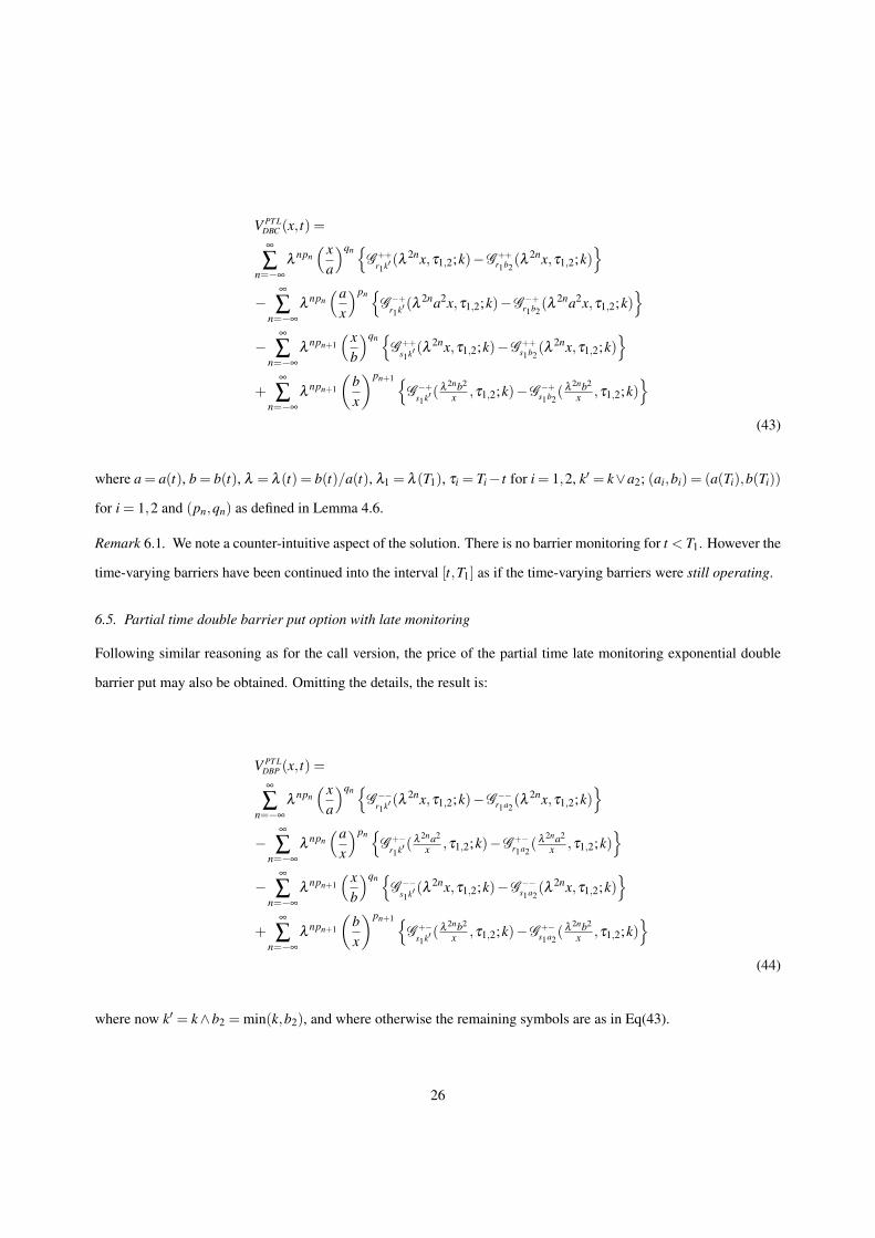
6.5. Partial time double barrier put option with late monitoring
Following similar reasoning as for the call version, the price of the partial time late monitoring exponential double
barrier put may also be obtained. Omitting the details, the result is:
V PT LDBP (x, t) =∞
∑n=−∞
λnpn( x
a
)qn {G −−r1k′ (λ
2nx,τ1,2;k)−G −−r1a2(λ 2nx,τ1,2;k)
}−
∞
∑n=−∞
λnpn(a
x
)pn {G +−
r1k′ (λ 2na2
x ,τ1,2;k)−G +−r1a2
(λ 2na2
x ,τ1,2;k)}
−∞
∑n=−∞
λnpn+1
( xb
)qn {G −−s1k′ (λ
2nx,τ1,2;k)−G −−s1a2(λ 2nx,τ1,2;k)
}+
∞
∑n=−∞
λnpn+1
(bx
)pn+1 {G +−
s1k′ (λ 2nb2
x ,τ1,2;k)−G +−s1a2
(λ 2nb2
x ,τ1,2;k)}
(44)
where now k′ = k∧b2 = min(k,b2), and where otherwise the remaining symbols are as in Eq(43).
26
n Term Cumulative Sum-3.0000 0.0000 0.0000-2.0000 0.0000 0.0000-1.0000 0.0000 0.00000.0000 28.0073 28.00731.0000 -5.2027 22.80462.0000 0.0000 22.80463.0000 0.0000 22.8046
(46)
Table 1: Evaluation of terms in Eq(43) for the partial-time late monitoring double barrier call. ‘Term’ is the value of the n-th term under thesummation in Eq(43), and ‘Cumulative Sum’ gives the approximate price.
7. Computations
In this section we present numerical computations for our formulae from Section 6. As will be demonstrated, con-
vergence for the doubly-infinite sums in our formulae is very rapid. We consider the following choice of parameters
representing expiry times, risk-free rates and stock price volatilities.
ParameterValues
T1 T2 x k r σ
1/12 1/6 1000 1000 0.05 0.20
(45)
Namely, we consider one-month early and late partial-barrier monitoring windows t ∈ [0,T1] and t ∈ [T1,T2] respect-
ively struck at k.
In (46) we demonstrate the numerical evaluation of Eq(43) with the above parameters, and for the choices A= 850;B=
1150;α = −0.0150;β = 0.0150. ‘Term’ is the value of the n-th term in the summation in Eq(43), and ‘Cumulative
Sum’ gives the cumulative approximation of the price.
In general the numerical evaluation of our formulae only requires a few terms on either side of the n = 0 term.
Figure 1 displays the results of computations for the partial-time early monitoring double-barrier call (labelled EM)
given by Eq(38) and the late monitoring double barrier call Eq(43) (labelled LM) as a function of the current stock
price x for the above choices for the other parameters. For comparison the dashed line indicates the standard double
barrier call price given by Eq(28), with upper and lower monitoring windows extending over the full life of the option
t ∈ [0,T2]. Figure 2 displays the equivalent results for the puts given by Eq(39), Eq(44) and Eq(29) respectively.
As expected, for all values of x the restriction of the monitoring to a subset of the option lifetime increases option
values, with both the early and late monitoring values lying wholly above the dashed lines. The largest effect occurs
27
Figure 1: Eq(38), (43) and (28)
in the case of the Early Monitoring (EM) windows.
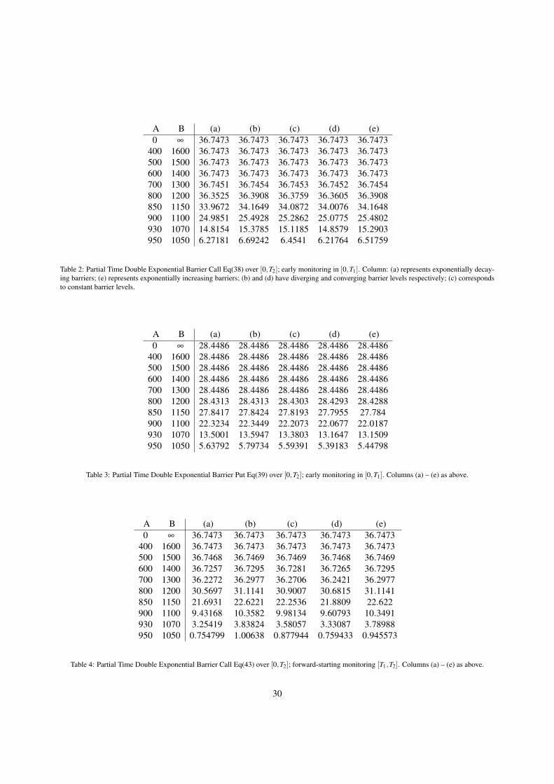
We conclude our numerical evaluations by considering different pairs of values for (A,B) and several choices of
(α,β ) for exponential barrier levels as given in (47) labelled (a) to (e). Numerical computations for these choices
of the exponential parameters in the corresponding columns are provided in the tables. They are chosen to coincide
with those used in Kunitomo and Ikeda (1992) and Buchen and Konstandatos (2009) after accounting for notational
differences, where corresponding tables in the case of full-window monitoring for Eq(28) and Eq(29) may also be
found.
(a) (b) (c) (d) (e)
α −0.010 −0.010 0 +0.010 +0.015
β −0.015 +0.010 0 −0.010 +0.010
(47)
For each table of numerical computations below column (a) represents the numerical results for exponentially decay-
ing barriers, column (e) represents exponentially increasing barriers. Columns (b) and (d) represent diverging and
28
Figure 2:
converging barrier levels respectively. Column (c) corresponds to constant ( i.e. ‘flat’ or non - time-varying) barrier
levels. The case (A = 0, B = ∞) corresponds to standard vanilla options, namely without any barriers. We evaluated
our formulae for the choice of parameters in 45. The tables illustrate the effects of the time-varying barriers compared
to the constant barriers in (c). We included tables for both the calls and puts for completeness.
29
A B (a) (b) (c) (d) (e)0 ∞ 36.7473 36.7473 36.7473 36.7473 36.7473
Table 5: Partial Time Double Exponential Barrier Put Eq(44) over [0,T2]; forward-starting monitoring [T1,T2]. Columns (a) – (e) as above.
8. Conclusion
In contrast to other methods our approach allowed us to directly obtain pricing formulae for all the exponential and
time-varying single and double barrier options we considered without the need for a single integration against an
equivalent martingale measure nor the complicated joint density of the underlying stock price and the maximum and
minimum. Our analysis was conducted directly in the original asset and time variables without the need for either
variable transformations, or transformations into Fourier space.
In the single exponential and time varying barrier case, the prices of all the related barrier options we considered
with either full monitoring or partial monitoring barrier windows whether with knock-out or knock-in boundaries, are
related via a set of image function parity relations which we presented. The use of the parity relations allowed all
the option prices to be expressed solely in terms of portfolios created from a single first-order European Gap option
instrument and it’s mathematical images with respect to the exponentially time-varying barrier.
We provided proofs for a new set of lemmas allowing us to extend the results of Buchen and Konstandatos (2009) for
31
simultaneous lower and upper exponential and time-varying barrier levels to where the monitoring window extends
to a subset of the lifetime of the option. They allowed the efficient analytical treatment of the single and double
barrier options with late-monitoring windows, and also required a second-order variant of the European Gap option
instruments which may be interpreted as generalised compound options. It is a rather remarkable result that all the
barrier options we considered, regardless of the monitoring window, have prices which can be expressed solely in
terms of a single family of Gap options.
The intermediate result of the decomposition of the partial barrier and double barrier option prices into first and second
order Gap options is essentially model independent, and as far as we know are new.
Our approach may be readily used to treat any sequence of late-starting double exponential and time-varying barrier
monitoring windows. Although we did not treat the problem of credit default modelling explicitly, we note that credit
default modelling naturally requires lower and upper exponential and time-varying barrier levels on the value of a
firm. The techniques and results of this work particularly in the late monitoring double barrier case point a way to
getting tractable solutions in a multi-barrier context for credit default modelling when using proper Black-Scholes
dynamics in contrast to modelling firm value using a simple Wiener process as the latent variable driving default.
AppendixA. Gap Options
Many exotic options can be priced entirely in terms of simpler ‘building block’ derivatives. For example Buchen
(2004) demonstrated such decompositions for some examples of path-independent dual-expiry options. More details
can be found in Konstandatos (2008) or more recently in Buchen (2012). We undertake a similar approach here,
however our analysis requires so-called gap options, for which the the option payoff is decoupled from the exercise
condition.
First order Gap options essentially standard European calls and puts with the exception that their strike and exercise
prices are allowed to differ. Second order gap options are are compound first order Gap options, and may be considered
as simple generalisations of the standard compound options of Geske (1979) and of the framework of Buchen (2004).
Gap options have also been referred in the literature as threshold options. These building blocks are the only ones
needed to construct the prices of all the exotic barrier options considered in this paper.
AppendixA.1. First-order Gap Options
We define the first-order gap option of exercise price ξ and strike price k, denoted by G sξ(x,τ;k), where τ = (T − t),
as the price of a European derivative security with expiry T payoff:
G sξ(x,0;k) = (x− k)I(sx>sξ ) (A.1)
32
Here s = ±1 indicates the type of gap option: e.g. s = +1 indicates an ‘up-type’ gap option with exercise condition
x > ξ . Conversely s = −1 indicates a ‘down-type’ with exercise condition x < ξ . The gap is defined to be |ξ − k|,
the absolute difference between the exercise and strike prices. Under Black-Scholes dynamics the price of such
instruments for t < T is expressible in terms of the uni-variate normal distribution function:
G sξ(x,τ;k) = xN (sdξ )− ke−rτN (sd′
ξ) (A.2)
where [dξ ,d
′ξ
]= [log(x/ξ )+(r± 1
2 σ2)τ]/σ
√τ
Clearly, a vanilla call of strike price k and time τ = (T − t) remaining to expiry has zero gap and price given by
Ck(x,τ) = G+k (x,τ;k). Similarly, a corresponding vanilla put with zero gap has price Pk(x,τ) =−G−k (x,τ;k).
AppendixA.2. Second-order Gap Options
To define the required higher-order building blocks, consider the scenario of two dates T1,T2 with T1 < T2 and let
τi = (Ti− t) and τ = (T2−T1). The second-order gap option Gs1s2
ξ1ξ2(x,τ1,τ2;k) is defined such that at time T1 it pays a
first order gap option Gs2
ξ2(x,τ;k) with time τ remaining to expiry, provided the stock price at time T1 is either above
or below some expiry price ξ1. The second-order gap option’s T1 payoff is therefore:
Gs1s2
ξ1ξ2(x,0,τ;k) = G
s2ξ2(x,τ;k) · I(s1x>s1ξ1) (A.3)
where si =±1.
It is also useful to write down the payoff of this second-order gap option at time T2. From (A.1) this payoff is
Gs1s2ξ1ξ2
(x1,x2;k) = (x2− k)I(s1x1>s1ξ1)I(s2x2>s2ξ2) (A.4)
where xi = X(Ti). Thus the second-order gap option requires its holder to buy one unit of the underlying asset at
time T2 for k (dollars), but only if the asset price at time T1 is above (or below) the exercise price ξ1 and if the asset
price at time T2 is above (or below) the exercise price ξ2. There are four different types of second-order gap options
corresponding to the choice of signs for (s1,s2).
To simplify notation somewhat, we shall write τ1,2 for the pair (τ1,τ2). The price of second-order gap option, under
Black Scholes dynamics, is readily expressible in terms of the bi-variate normal distribution as
Gs1s2
ξ1ξ2(x,τ1,2;k) = xN (s1d1,s2d2; s1s2ρ)− k e−rτ2N (s1d′1,s2d′2; s1s2ρ) (A.5)
33
where τi = Ti− t, ρ =√
τ1/τ2 and
[di,d′i
]= [log(x/ξi)+(r± 1
2 σ2)τi]/σ
√τi
A proof is omitted however the result follows under discounted expectations. Second-order gap options are examples
of generalised compound options.
Acknowledgements
I would like to thank Dr Clare Louise Chapman for proofreading this document and for helpful comments and sug-
gestions. I would also like to thank Associate Professor Peter W. Buchen and Professor Erik Schlogl for fruitful
discussions regarding aspects of this work.
Black, F. and Cox, J. (1976). Valuing corporate securities: Some effects of Bond Indenture Provisions. Journal of Finance, 31(2):351–367.
Black, F. and Scholes, M. (1973). The pricing of options and corporate liabilities. Journal of Political Economy, 81:637–654.
Buchen, P. (2001). Image options and the road to barriers. Risk Magazine, 14(9):127–130.
Buchen, P. (2004). The pricing of dual-expiry exotics. Quantitative Finance, 4(1):101–108.
Buchen, P. (2012). An Introduction to Exotic Option Pricing. CRC Press, Taylor & Francis Group, United States of America.
Buchen, P. and Konstandatos, O. (2009). A New Approach to Pricing Double Barrier Options with Arbitrary Payoffs and Curved Boundaries.
Applied Mathematical Finance, 16(6):497–515.
Carr, P. (1995). Two extensions to barrier option valuation. Applied Mathematical Finance, 2(3):173–209.
Fusai, G., Abrahams, I. D., and Sgarra, C. (2006). An exact analytical solution for discrete barrier options. Finance and Stochastics, 10(1):1–26.
Geman, H. and Yor, M. (1996). Pricing and Hedging Double-Barrier Options: A Probabilistic Approach. Mathematical Finance, 6(4):365–378.
Geske, R. (1979). The valuation of compound options. Journal of Finanancial Economics, 7:63–81.
Goldman, M., Sosin, H., and Gatto, M. (1979). Path dependent options: buy at the low, sell at the high. Journal of Finance, 34(5):1111–1127.
Gupton, G., Finger, C., and Bhatia, M. (1997). Introduction to creditmetrics. [Online: http://homepages.rpi.edu/ guptaa/MGMT4370.09/Data/CreditMetricsIntro.pdf].
Harrison, J. and Pliska, S. (1981). Martingales and stochastic integrals in the theory of continuous trading. Stochastic Processes and their
Applications, 11:215–260.
Harrison, J. and Pliska, S. (1983). Stochastic calculus model of continuous trading: complete markets. Stochastic Processes and their Applications,
15:313–316.
Heynen, R. and Kat, H. (1994). Partial barrier options. Journal of Financial Engineering, 3(3/4):253–274.
Howison, S. and Steinberg, M. (2007). A Matched Asymptotic Expansions Approach to Continuity Corrections for Discretely Sampled Options.
Part 1: Barrier Options. Applied Mathematical Finance, 14(1):63–89.
Hsiao, Y.-L. (2012). Closed-form approximate solutions of window barrier options with term structure volatility and interest rates using the
boundary integral method. Journal of Mathematical Finance, 2:291–302.
Hui, C. (1997). Time-dependent barrier option values. The Journal of Futures Markets, 17(6):667–688.
Konstandatos, O. (2003). A new framework for pricing barrier and lookback options. PhD thesis, The University of Sydney.
Konstandatos, O. (2008). Pricing path dependent options: a comprehensive mathematical framework. Applications of Mathematics. VDM-Verlag
Dr Mueller Aktiengesellschaft & Co. Kg, Saarbr first edition.
34
Kunitomo, N. and Ikeda, M. (1992). Pricing options with curved boundaries. Mathematical Finance, 2:276–298.
Merton, R. (1973). Theory of rational option pricing. Bell Journal of Economics and Management Science, 4(1):141–183.
Merton, R. (1974). On the pricing of corporate debt: the risk structure of interest rates. Bell Journal of Finance, (1):449–470.
Pelsser, A. (2000). Pricing Double Barrier Options using Laplace Transforms. Finance and Stochastics, 4(1):95–104.
Rich, D. (1994). The mathematical foundations of barrier option pricing theory. Advances in Futures and Operations Research, 7:267–311.
Rubinstein, M. and Reiner, E. (1991). Breaking down the barriers. Risk Magazine, 4(8):28–35.
Zhang, P. (1998). Exotic options: A guide to second generation options. World Scientific Press, Singapore.