99
Methods for Calculating the Sharpe Ratio Diploma Thesis by Rahel Berkemann FACULTY FOR MATHEMATICS AND PHYSICS MATHEMATICAL INSTITUTE Date: June 12, 2006 Supervisor: Prof. Dr. L. Gr¨ une
| Date post: | 05-May-2018 |
| Category: |
Documents |
| Upload: | nguyencong |
| View: | 245 times |
| Download: | 1 times |

Methods for Calculating theSharpe Ratio
Diploma Thesis
by
Rahel Berkemann
FACULTY FOR MATHEMATICS AND PHYSICS
MATHEMATICAL INSTITUTE
Date: June 12, 2006 Supervisor:Prof. Dr. L. Grune

Acknowledgements
First of all I would like to thank Prof. Grune for his supervision.A special thank you to my family, especially my mom and my grandfatherfor financial and moral support. Last but not least I have to mention MissHarper, Mr Hanscher and Mr Worthmann for not only being there but alsosupporting me in every respect.A very special thank you to Mr Seppeur for his motivation, advice and kind-ness.
i
Contents
1 Introduction 1
2 Preliminaries 4
2.1 Introduction to Probability Theory . . . . . . . . . . . . . . . 4
2.2 Stochastic Growth Model . . . . . . . . . . . . . . . . . . . . . 13
3 Stochastic Growth Model and Financial Measures 18
4 Reference Model 23
4.1 The Model . . . . . . . . . . . . . . . . . . . . . . . . . . . . . 23
4.2 The Optimal Value and Control Function . . . . . . . . . . . . 24
4.3 The Dynamics in the Long Run . . . . . . . . . . . . . . . . . 28
5 Time Series Approach 30
5.1 Random Number Generators . . . . . . . . . . . . . . . . . . . 30
5.2 Solving the model . . . . . . . . . . . . . . . . . . . . . . . . . 32
5.3 Sharpe Ratios subject to initial values . . . . . . . . . . . . . 37
6 Random Variable Approach 42
6.1 Restrictions on ε . . . . . . . . . . . . . . . . . . . . . . . . . 42
ii

CONTENTS iii
6.2 Sharpe Ratios subject to initial values . . . . . . . . . . . . . 44
7 Comparison 47
7.1 Programme Check . . . . . . . . . . . . . . . . . . . . . . . . 48
7.2 Correlations . . . . . . . . . . . . . . . . . . . . . . . . . . . . 50
7.3 σε and Model Outcomes . . . . . . . . . . . . . . . . . . . . . 53
8 Asset Pricing with Loss Aversion 58
8.1 Our Reference Model and Loss Aversion . . . . . . . . . . . . 58
8.2 Loss Aversion and Financial Measures . . . . . . . . . . . . . 60
8.3 Solution . . . . . . . . . . . . . . . . . . . . . . . . . . . . . . 61
9 Summary and Conclusion 64
A Matlab Codes 66
A.1 MATLAB codes for Path k . . . . . . . . . . . . . . . . . . . . 66
A.2 MATLAB codes for the Time Series solution . . . . . . . . . . 70
A.3 MATLAB codes for the Random Variable solution . . . . . . . 74
A.4 MATLAB codes for the Check . . . . . . . . . . . . . . . . . . 78
A.5 MATLAB codes for Correlations . . . . . . . . . . . . . . . . . 81
A.6 MATLAB code for the Loss Aversion model . . . . . . . . . . 86
B The included CD 88
List of Figures
4.1 k-components of optimal trajectories for z(0) = −0.32, 0, 0.32 29
5.1 Paths for y and z . . . . . . . . . . . . . . . . . . . . . . . . . 33
5.2 Path for capital k and consumption c . . . . . . . . . . . . . . 33
5.3 The stochastic discount factor m . . . . . . . . . . . . . . . . 34
5.4 The price p . . . . . . . . . . . . . . . . . . . . . . . . . . . . 36
5.5 The gross return R . . . . . . . . . . . . . . . . . . . . . . . . 36
6.1 density function of ε in [−0.5, 0.5] . . . . . . . . . . . . . . . . 43
6.2 density function of ε in [−0.05, 0.05] . . . . . . . . . . . . . . . 43
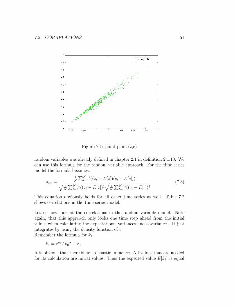
7.1 point pairs (z,c) . . . . . . . . . . . . . . . . . . . . . . . . . . 51
7.2 density function of ε in [−0.5, 0.5], σε = 0.01 . . . . . . . . . . 53
iv
List of Tables
5.1 Sharpe Ratios depending on initaial values . . . . . . . . . . . 41
6.1 Sharpe Ratios depending on initial values . . . . . . . . . . . . 46
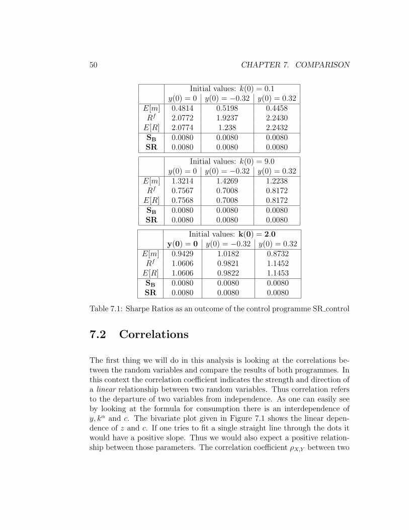
7.1 Sharpe Ratios as an outcome of the control programme SR control 50
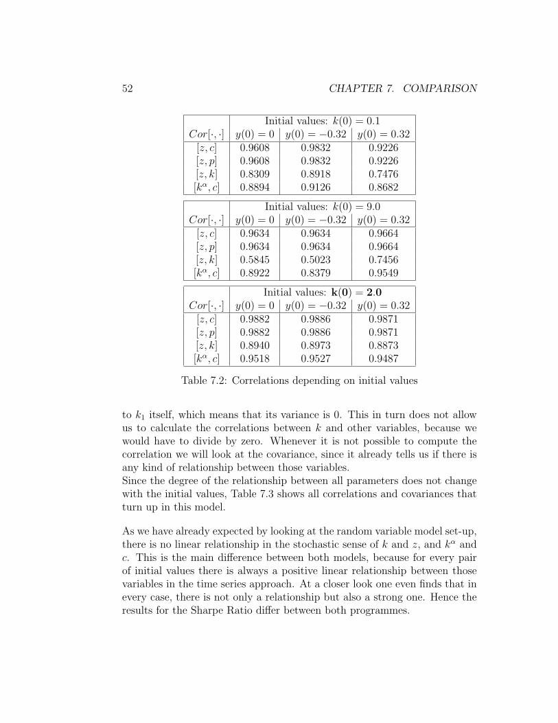
7.2 Correlations depending on initial values . . . . . . . . . . . . . 52
7.3 Correlations and Covariances in the RV model . . . . . . . . . 53
7.4 Results for the Sharpe Ratio, σε = 0.01, N = 50000, ε ∈[−0.05, 0.05] . . . . . . . . . . . . . . . . . . . . . . . . . . . . 54
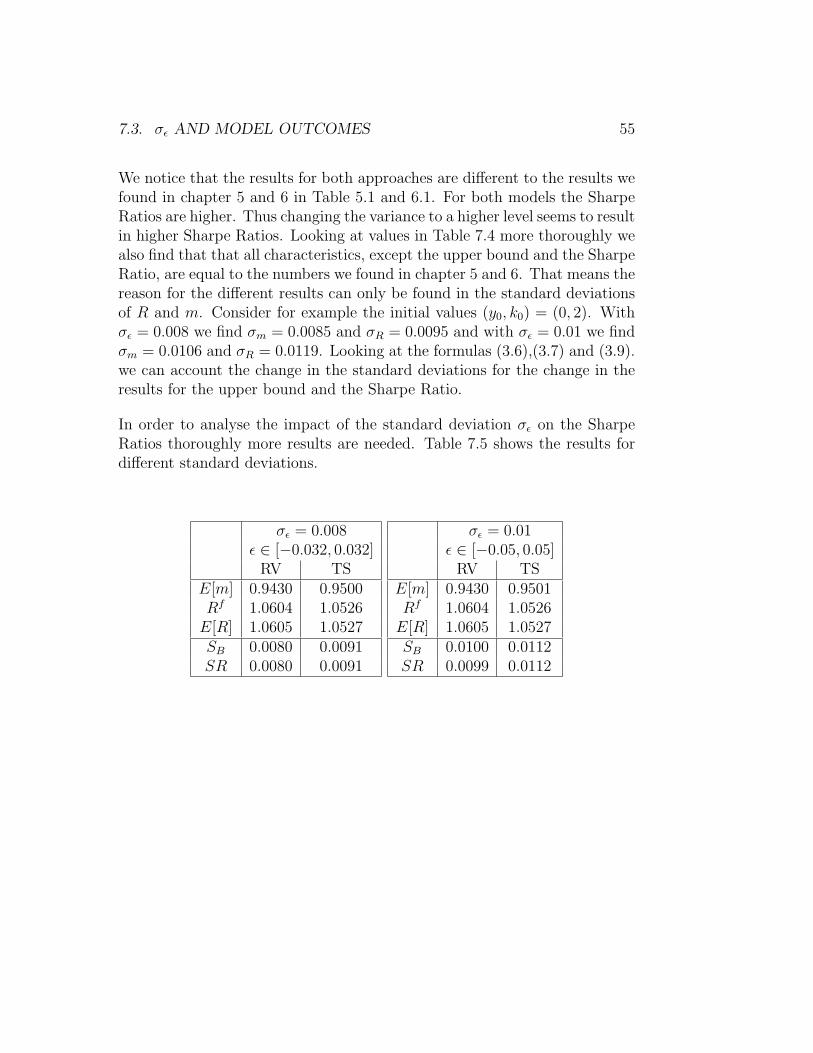
7.5 Sharpe Ratios depending on σε, N = 50000, (y0, k0) = (0, 2) . 56
7.6 Sharpe Ratio ratios . . . . . . . . . . . . . . . . . . . . . . . . 56
8.1 Results for varying b0 . . . . . . . . . . . . . . . . . . . . . . . 63
8.2 Results for varying b0 as in Gune and Semmler . . . . . . . . . 63
v

Chapter 1
Introduction
There are several methods for pricing asset characteristics such as the risk-free interest rate, the return of risky assets and Sharpe Ratios. In this thesisthe underlying model is always a stochastic growth model. Even when we arerestricted to a certain model there are still different approaches for solvingfor the financial measures, such as the Time Series, the Random Variable andthe Stochastic Dynamic Programming approach. The purpose of this thesisis to compare the outcome of those approaches with each other when appliedto the same model. In this thesis the time series and the random variable ap-proach are computed but not the stochastis dynamic programming approach.The results for the latter can be found in Grune and Semmler, Solving AssetPricing Models with Stochastic Dynamic Programming [7].
Since we will work with a stochastic growth model, which means we workwith a model where we do not obtain certain outcomes but usually variouspossible ones, the concepts of random variables, expected values, etc. areextensively used throughout this paper. Thus chapter 2 will give an intro-duction to probability and distribution theory. It will also describe the basicfeatures of stochastic growth models as used throughout the following chap-ters.
Since we want to solve the model for asset price characteristics, we haveto close the gap between the consumption paths we find when solving thestochastic growth models and the parameters we need for calculating thefinancial measures. The intention of chapter 3 is to explain how we get from
1

2 CHAPTER 1. INTRODUCTION
the basic pricing equation, which is nothing else but the first order conditionfor an optimization problem, to measures such as the risk-free interest rate,etc.. We will also find that knowing a consumer’s stochastic discount factoris sufficient for the calculation of at least an upper bound for the SharpeRatio.
In chapter 4 the reference model as was used in the underlying paper, thatis Grune and Semmler, Solving Asset Pricing Models with Stochastic Dy-namic Programming [7], is introduced. This model is consumption basedwith labour augmenting shocks and given dynamics for the capital devel-opment over time. It can be solved analytically. Looking at the capitaldynamics in the long run we will discover that independent of starting valuesthe capital will start to oscillate around some sort of ”equilibrium point”at an early point in time . Thus one assumes that the financial measurescalculated from this model will also converge quickly to some ”equilibrium”.
Chapter 5, which introduces the time series approach will show, that theassumed convergence behaviour of the Sharpe Ratio cannot be found. Infact, we will find that we have to look very far ahead of the starting point intime before we get at least some kind of ”equilibrium”. But even then thedifference between the outcome of our approach compared to the one of thestochastic dynamic programming approach, is obvious.
In chapter 6 the last approach is introduced. Since we will work with theconcept of random variables, all information about the distributions are used.In comparison with the results of the stochastic dynamic programming ap-proach the results we obtain in this context are nearly equal.
Having obtained all results needed to compare the models with each other,and having seen that the outcomes vary rather a lot, chapter 7 will now lookfor differences in the programmes and approaches. Since the results of therandom variable approach are equal to the results of the stochastic dynamicprogramming approach, this chapter is focussing on explaining the differencesbetween the random variable and time series model. We will start with ver-ifying the time series programm for accurateness. The next section will lookfor correlations between various parameters of the underlying growth modeland will then look in how far the correlations differ from approach to ap-proach. Having figured out that there are differences, we will test the impact

3
of a change of the standard deviation of our shock variable on the modeloutcomes.
Reality shows that consumption based models do not fit financial marketcharacteristics to time series data. Therefore asset pricing models with theadditional preference of loss aversion were recently proposed by behaviouralfinance. Thus in chapter 8 we have a closer look at a growth model also in-cluding the concept of loss aversion. Consumers are here assumed to becomemore careful with every loss they experience. In order to fit this concept intoour basic stoachstic growth model, we have to adjust the model for a factorthat reacts on gains or losses the consumer experiences. Since the financialmeasures have to give considerations to this adjustment, we will re-define theformulas we use for the calculation of the asset price characteristics. In thelast section we will compare the results gained from a time series approach tosolve that model for Sharpe Ratios with the results obtained by the stochas-tic dynamic programming as can be found in Grune and Semmler, SolvingAsset Pricing with Loss Aversion [8].
Finally we will summarize and conclude the results found in the previouschapters.
The Appendix will cover the MATLAB codes used for computation and itwill give an overview of the included CD.

Chapter 2
Preliminaries
We will begin this chapter with the introduction to probability and distribu-tion theory. These concepts are essential for the different methods we use forsolving the underlying model for the asset price characteristics. Furthermorewe will define the basic concepts of the stochastic growth model such as theMarginal Utility of Consumption.
2.1 Introduction to Probability Theory
Because of the uncertainty about future payoffs that stochastic growth mod-els try to capture we need formal definitions of stochastic variables, i.e. theExpected Value, the Standard deviation, etc. Therefore it is necessary togive a brief introduction to probability theory as in Greene’s EconometricAnalysis [6], chp. 3 and 4.
Definition 2.1.1 (Random Variable).A Random Variable X : Ω → R is a function from an ”event space” Ω to R.Its realizations or outcomes will be denoted by x. The probability measureis associated with X so that subsets of Ω are assigned a probability P (Ω). Inother words: Until the experiment is performed it is unknown what value Xwill take. Therefore probabilities are associated with realizations to quantifythis uncertainty. The probability that X takes a certain value is denoted asP(X=x).
4

2.1. INTRODUCTION TO PROBABILITY THEORY 5
A random variable is said to be discrete if the set of outcomes is either finitein number or countably infinite. The random variable is continuous if the setof outcomes is uncountable.
Definition 2.1.2 (Probability Distribution).A probability distribution denoted as f(x) is a listing of values taken by arandom variable X and their associated probabilities.For a discrete random variable,
f(x) = P (X = x). (2.1)
The axioms of probability require that
1. 0 ≤ P (X = x) ≤ 1.
2.∑
x
f(x) = 1.
For the continuous case, we can only assign positive probabilities to intervalsin the range of x, because the probability associated with any particular pointis zero. The probability density function (pdf) is defined so that f(x) ≥ 0and
1. P (a ≤ x ≤ b) =
∫ b
a
f(x)dx ≥ 0.
The result is the area under f(x) in the interval from a to b. The axioms ofprobability require that
2.
∫ ∞
−∞f(x)dx = 1.
It is possible that the range of x is not infinite. In that case f(x) = 0 isdefined anywhere outside the appropriate range.
Definition 2.1.3 (Cumulative Distribution Function).Let x be a random variable. The probability that x is less than or equal toa is denoted F (a). F (x) is called cumulative distribution function (cdf).For a discrete random variable,
F (x) =∑X≤x
f(x) = P (X ≤ x). (2.2)
6 CHAPTER 2. PRELIMINARIES
For a continuous variable,
F (x) =
∫ x
−∞f(t)dt.
For the discrete as well as for the continuous random variable, the cdf has tosatisfy the following properties:
1. 0 ≤ F (x) ≤ 1.
2. If x > y, then F (x) ≥ F (y).
3. F (+∞) = 1.
4. F (−∞) = 0.
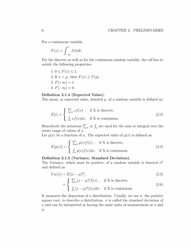
Definition 2.1.4 (Expected Value).The mean, or expected value, denoted µ, of a random variable is defined as:
E[x] =
∑
x xf(x) , if X is discrete,∫xxf(x)dx, if X is continuous.
(2.3)
Henceforth the notations∑
x or∫
xare used for the sum or integral over the
entire range of values of x.Let g(x) be a function of x. The expected value of g(x) is defined as:
E[g(x)] =
∑
x g(x)f(x) , if X is discrete,∫xg(x)f(x)dx, if X is continuous.
(2.4)
Definition 2.1.5 (Variance, Standard Deviation).The Variance, which must be positive, of a random variable is denoted σ2
and defined as:
V ar[x] = E[(x− µ)2] (2.5)
=
∑
x(x− µ)2f(x) , if X is discrete,∫x(x− µ)2f(x)dx, if X is continuous.
(2.6)
It measures the dispersion of a distribution. Usually, we use σ, the positivesquare root, to describe a distribution. σ is called the standard deviation ofx and can be interpreted as having the same units of measurement as x andµ.

2.1. INTRODUCTION TO PROBABILITY THEORY 7
There are some important results that simplify the computation of the ex-pected value and the variance.
Theorem 2.1.6. Let X be a random variable.
1. The computation of the variance is simplified by using the followingequation:
V ar[X] = E[X2]− µ2 (2.7)
2. For constants a and b:
E[a + bX] = a + bE[X], (2.8)
which implies, for any constant a, that E[a] = a.
3. For constants a and b:
V ar[a + bX] = b2V ar[X], (2.9)
which implies, for any constant a, that V ar[a] = 0.
Proof: Theorem 2.1.5.Consider the discrete case, the continuous one is analogous.
1.
V ar[x] =∑
x
(x− µ)2f(x)
=∑
x
(x2 − 2xµ + µ2)
=∑
x
x2f(x)︸ ︷︷ ︸=E[x2]
−2µ∑
x
xf(x)︸ ︷︷ ︸=µ
+µ2∑
x
f(x)︸ ︷︷ ︸=1
= E[x2]− 2µ2 + µ2 = E[x2]− µ2

8 CHAPTER 2. PRELIMINARIES
2.
E[a + bx] =∑
x
(a + bx)f(x)
= a∑
x
f(x)︸ ︷︷ ︸=1
+b∑
x
xf(x)︸ ︷︷ ︸=E[x]
= a + bE[x]
3.
V ar[a + bx] = E[(a + bx)2]︸ ︷︷ ︸=E[a2+2abx+b2x2]
−E[a + bx]2︸ ︷︷ ︸(=a+bE[x])2
= a2 + 2abE[x] + b2E[x2]− a2 − 2abE[x]− b2E[x]2
= b2(E[x2]− E[x]2)
= b2V ar[x]
In our stochastic growths model we will work with two random variables.It is therefore useful to introduce the joint density function, the conditionalmean and the conditional variance.Let X and Y be two random variables. The joint density function, f(x, y),satisfies:
P (a ≤ x ≤ b, c ≤ y ≤ d) =
∑
a≤x≤b
∑c≤y≤d f(x, y), discrete case,∫ b
a
∫ d
cf(x, y)dxdy , continuous case.
(2.10)
The requirements that go along with the requirements in the univariate case,are:
f(x, y) ≥ 0 ,∑x
∑y f(x, y) = 1 , if X and Y are discrete,∫
x
∫yf(x, y)dxdy = 1, if X and Y are continuous.
(2.11)
2.1. INTRODUCTION TO PROBABILITY THEORY 9
We need the definition for the marginal probability distribution in order todefine expectations in a joint distribution.
Definition 2.1.7 (Marginal Probability Density).The marginal probability density is also called marginal probability distribu-tion. It is defined with respect to an individual variable and obtained fromthe joint distribution by summing or integrating out the other variable.
fx(x) =
∑
y f(x, y) , in the discrete case,∫yf(x, s)ds, in the continuous case.
(2.12)
Analogous for fy(y).
Definition 2.1.8 (Expected Values and Variances in a Joint Distri-bution).Let X and Y be random variables. Means and Variances of the variables arecalculated with respect to the marginal distributions. For the mean of x ina discrete distribution,
E[x] =∑
x
xfx(x) (2.13)
=∑
x
x
[∑y
f(x, y)
](2.14)
=∑
x
∑y
xf(x, y) (2.15)
The means of a variable in the continuous case are defined likewise, usingintegration instead of summation.The computation of variances works in the same manner:
V ar[x] =∑
x
(x− E[x])2f(x) (2.16)
=∑
x
∑y
(x− E[x])2f(x, y). (2.17)
Similarly for the continuous case, again using integration.
10 CHAPTER 2. PRELIMINARIES
Definition 2.1.9 (Covariance and Correlation).Let X and Y be random variables. For any function g(x, y),
E[g(x, y)] =
∑
x
∑y g(x, y)f(x, y) , in the discrete case∫
x
∫yg(x, y)f(x, y)dydx, in the continuous case.
(2.18)
The covariance of x and y is:
Cov[x, y] = E[(x− µx)(y − µy)] (2.19)
= E[xy]− µxµy (2.20)
= σxy. (2.21)
For the analysis the sign of the covariance is important, because it will in-dicate the direction of the covariation of X and Y. Consider an investmentstrategy that covaries positively with consumption, i.e. if consumption goesup, so does the revenue of the investment strategy. This sort of investmentwould not save from loss if income decreases and, as a result of it, consump-tion decreases.Since the magnitude of the covariation depends on the scales of measurement,the preferable measure is the correlation coefficient.
Definition 2.1.10 (Correlation Coefficient).The correlation coefficient has the same sign as the covariance but is unaf-fected by any scaling of the variables. Hence its value is always between −1and 1.
r[x, y] = ρxy (2.22)
=σxy
σxσy
, (2.23)
where σx and σy are the standard deviations of x and y, respectively.
In econometric modelling, conditioning and the use of conditional distribu-tions play a pivotal role. Again, we will just consider the bivariate case.
Definition 2.1.11 (Conditional Distribution).There is a conditional distribution over y for each value of x. The conditional

2.1. INTRODUCTION TO PROBABILITY THEORY 11
densities are:
f(y | x) =f(x, y)
fx(x)(2.24)
and
f(x | y) =f(x, y)
fy(y). (2.25)
Definition 2.1.12 (Conditional Mean and Conditional Variance).The conditional mean is the mean of the conditional distribution:
E[y | x] =
∑
y yf(y | x), if y is discrete∫yyf(y | x) , if y is continuous.
(2.26)
The conditional mean is also called the regression of y on x.
Similar to the mean, the conditional variance is the variance of the con-ditional distribution:
V ar[y | x] = E[(y − E[y | x])2 | x] (2.27)
=
∫y
(y − E[y | x])2f(y | x)dy, if y is continuous (2.28)
or (2.29)
V ar[y | x] =∑
y
(y − E[y | x])2f(y | x), if y is discrete. (2.30)
Again, the computation can be simplified by:
V ar[y | x] = E[y2 | x]− (E[y | x])2. (2.31)
Definition 2.1.13 (σ-Algebra).Let Ω be a set. Then a σ-algebra F is a nonempty collection of subsets of Ωsuch that the following hold:
1. Ω ∈ F
2. if A ∈ F then Ac ∈ F , where Ac denotes the complement of A,
12 CHAPTER 2. PRELIMINARIES
3. if (An)n is a sequence of elements of F , then⋃
n An ∈ F .
If S is any collection of subsets of F , then we can always find a σ-algebracontaining S, namely the power set of Ω, P(Ω). By taking the intersection ofall σ-algebras containing S, we obtain the smallest such σ-algebra. We callthe smallest σ-algebra containing S, the σ-algebra generated by S.
Definition 2.1.14 (Borel sets).The Borel σ-algebra is defined to be the smallest σ-algebra generated by theopen sets in Ω.
Definition 2.1.15 (Independent and Identically distributed RandomVariables ).Let X and Y be random variables.
X and Y are independent ⇐⇒ f(x, y) = fx(x)fy(y) (2.32)
Remark 2.1.16. If two random variables X and Y are independent thentheir covariance is zero, that means they are uncorrelated. And for any twofunctions g1(x) and g2(y) then
E[g1(x)g2(y)] = E[g1(x)]E[g2(y)]. (2.33)
In order to look at the convergence behaviour of a sequence of random vari-ables xn, we will introduce the concept of convergence in distribution:
Definition 2.1.17 (Convergence in Distribution). Assume xn to be asequence of random variables and let xn have cdf Fn(x). xn converges indistribution to a random variable x if
limn→∞
|Fn(x)− F (x)| = 0
at all continuity points of F (x). F (x) is the cdf of x.
The basic form of the most important theorem in econometrics which helps todescribe the statistical properties of estimators when their exact distributionsare unknown, is given in the following theorem.

2.2. STOCHASTIC GROWTH MODEL 13
Theorem 2.1.18 (Central Limit Theorem).Let x1, . . . , xn be a random sample from a probability distribution with meanµ and finite variance σ2. Then for xn = 1
n
∑ni=1 xi the Lindbergh-Levy variant
for the mean of a univariate distribution holds. Formally:
√n(xn − µ)
d−→ N [0, σ2], (2.34)
where N [0, σ2] is the the normal distribution with mean 0 and standard
deviation σ.d−→ stands for the limiting distribution and means that if xn
converges in distribution to x, and F (x) is the cdf of x, then F (x) is thelimiting distribution of xn.
Thus√
n(xn − µ)d−→ N [0, σ2] can also be thought of representing the fact
that the relationship is an asymptotic one, i.e. with n increasing withoutboundary the distribution
√n(xn−µ) approaches the normal distribution of
with mean zero and variance σ2. See also A.W. Lo, [11], p.38..
2.2 Stochastic Growth Model
According to Mirman and Brock [2], we will introduce the basic stochasticgrowth model.One tradition of asset pricing models is based on the stochastic growth modelwith production. In these models it is crucial how consumption is modelled.The goal is to find an optimal consumption path in order to deduce thevalues of investment strategies. The randomness is assumed to occur in theproduction function of firms as labor augmenting technical progress. As aresult consumption and dividends can be assumed to be endogenous. Indealing in this uncertain context, we will maximize the expected sum ofdiscounted utilities.
Definition 2.2.1 (Utility of Consumption).Utility of Consumption, denoted u(c), is the welfare an individual gets byconsuming a certain amount of goods. We assume consumers to spend theiravailable income so as to maximize their utility function, u(·).
Definition 2.2.2 (Utility Function).The utility function u(·) is the expression economists use to show utility as
14 CHAPTER 2. PRELIMINARIES
a function of an individual’s consumption. We assume the utility, u(c), isincreasing in the quantity of each good consumed. We require the utilityfunction to fulfill the usual properties, that is:
u′ > 0, u′′ < 0.
The second property denotes concavity, which is important to express a con-sumer’s declining marginal value of additional consumption. To guaran-tee any consumption at all, we also require the utility function to satisfyu′(0) = +∞.
From now on time subscripts will be used only when necessary to explicitlydistinguish events in different periods.Consider a one sector growth model of an economy in discrete time withfuture production uncertainties. The production function for this economyis given by:
Yt = F (Kt, Lt; εt), (2.35)
where Yt, Kt and Lt are output, capital and labor at time t, respectively. εt isthe random variable representing uncertainty. As usual, we assume that ourproduction function has constant returns to scale in its first two arguments.That means, that multiplying both arguments by any nonnegative constantα causes output to change by the same factor.Formally, but without the time coefficient:
F (αL, αK; ε) = αF (L, K; ε), for all α ≥ 0. (2.36)
Because of the production function’s homogeneity of degree 1, we can workwith the production function in the following form. Let α = 1
L, we yield:
yt ≡Yt
Lt
= F (1,Kt
Lt
; εt) = f(kt, εt). (2.37)
Here kt is the economy’s capital stock per unit of labor and yt is output perunit of labor. kt is also called capital labor ratio.
Assumption 2.2.3 (Assumptions on f).Let ρ be the possible values of the random variable εt. f(·, ρ) is endowed
2.2. STOCHASTIC GROWTH MODEL 15
with the common properties of production functions.Thus we assume:
f(0, ρ) = 0,
f ′(·, ρ) > 0,
f ′′(·, ρ) < 0,
for all values of ρ. In addition, f(·, ρ) is assumed to satisfy the Inada condi-tions, namely:
f ′(0, ρ) = +∞,
f ′(∞, ρ) = 0,
for all values of ρ. Finally f and f ′ are continuous in k and ε jointly.
Now, take a closer look at the statistics of the random variable εt. Sincethe probability space (Ωt,Ft, Pt) is assumed to be the same in each period,time subscripts will be dropped for convenience and the state space willbe denoted by (Ω,F , P ). Here, let Ω be the ”event space”,the arbitrary,nonempty set of possible ”states of the world” that influence the productionfunction. ω ∈ Ω represents the occurence of an exogenous event that effectsthe production function. To be mathematically rigorous, let F be a collectionof subsets of Ω. The set F is a σ-algebra of subsets of Ω. P is supposed tobe a probability measure, i.e. P is a nonnegative σ-additive function on F .That means P (Ω) = 1, P (F ) = Σm
i=1P (Fi)∀F ∈ F and every finite partitionFi, i = 1, · · · , m of F in F and ∀F ∈ F is Fi, i = 1, 2, · · · , Fi 6= Fj ∀i 6=j,∪∞i=1Fi = F and ∪∞i=1 P (Fi) = P (F ).Thus the probability that the state of the world ω is an element of F is givenby
P (F ) = P [ω ∈ F ]. (2.38)
In order to translate random happenings in measurable values the randomvariable εt is introduced that takes our measure space (Ω,F , P ) into the realline (R,B), where B is the set of Borel sets defined as above.It is important to note that the random variables εt are assumed to be inde-pendent and identically distributed. This assumption is strongly simplifyingwhereas the assumption about the time independency of the measure spaceremains crucial to the limit theorem.ε : Ω → R generates a measure, ν(·), on the Borel subsets of the real line.
ν(z ∈ S) = Pω ∈ ε−1(S),
16 CHAPTER 2. PRELIMINARIES
where
ε−1(S) ∈ F for all S ∈ B,
and
ε−1(S) = ω : z(ω) ∈ S.
Thus the numerical random value z with associated measure ν(·) representsthe statistics of the random ”states of the wordl”.Output is either increased or decreased for all values of k by the randomevent ε. Moreover it is assumed that the random events are indexed in a wayas to have
∂f(k, ε)
∂ε> 0, for all k. (2.39)
Furthermore, it is assumed that the random event can only affect productionin a ”compact” way. In other words, numbers 0 < α < β < ∞ exist suchthat
ε ∈ [α, β]
and for all x > 0,
∞ > f(k, β) > f(k, α) > 0. (2.40)
Without loss of generality is it assumed that for every ρ > α, ν([α, ρ]) > 0.Since, if not, α = supη : ν([0, η]) = 0 could be chosen. Accordingly,ν([ρ, β]) > 0 for each ρ < β.Now, consider the growth process which is represented by the following dif-ference equation
ct + kt = f(kt−1, εt−1), (2.41)
where ct is an optimal consumption policy in the sense that consumption ischosen so as to maximize the expected sum of discounted utilities. We willalso assume an infinfite time horizon.
2.2. STOCHASTIC GROWTH MODEL 17
Definition 2.2.4 (Maximization Problem).In this set-up the maximization problem becomes:
max Et[∞∑
t=0
δtu(ct)] (2.42)
subject to the constraints
ct + kt = f(kt−1, εt−1), t = 1, 2, . . .
c0 + k0 = s, k0, c0 ≥ 0,
where s > 0 is the given initial data of the problem representing the his-torically given capital stock. δ is the subjective discount rate and it holds:δ ∈ (0, 1).
Consider the definition of β and the conditions that hold for the productionfunction. There exists a kβ so that for all k > kβ
f(k, β) < k.
Thus it is not possible to sustain capital independent from the state of theworld if k > kβ.
Chapter 3
Stochastic Growth Model andFinancial Measures
In the context of this paper we have to compute every financial measure withrespect to the set-up of a stochastic growth model. In order to get our for-mulas in the necessary way we look without loss of generality at a discrete,two period decision problem, cf Cochrane [4] p.6 - p.19. We will see thatevery infinite decision problem is equivalent to the two-period problem. Itis also always possible to look at the constraints to such a problem from theperspective of consumption.
Let us start with the two-period problem and derive the basic pricing equa-tion. For every maximization problem of the form:
maxξ
u(ct) + Et[βu(ct+1)]
subject to
ct = et − ptξ
ct+1 = et+1 + xt+1ξ,
where ξ denotes the fraction of income that is invested, et is the income ofperiod t and xt is period t’s payoff, the first order condition for an optimal
18
19
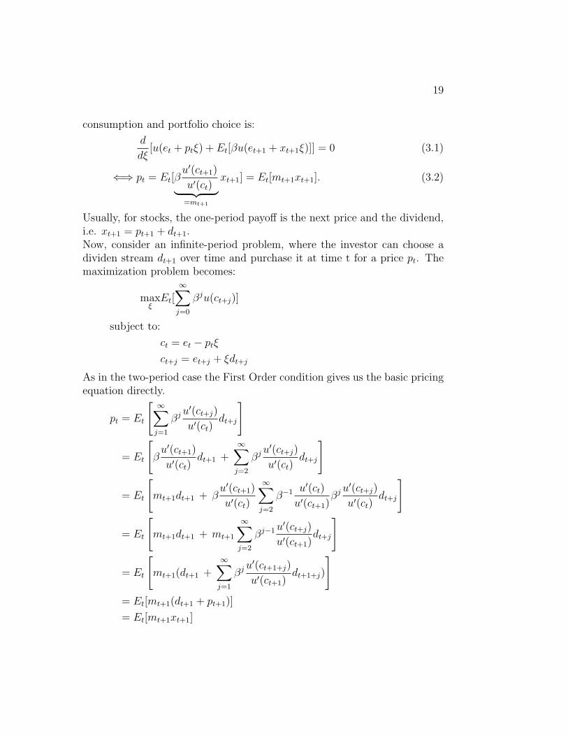
consumption and portfolio choice is:
d
dξ[u(et + ptξ) + Et[βu(et+1 + xt+1ξ)]] = 0 (3.1)
⇐⇒ pt = Et[βu′(ct+1)
u′(ct)︸ ︷︷ ︸=mt+1
xt+1] = Et[mt+1xt+1]. (3.2)
Usually, for stocks, the one-period payoff is the next price and the dividend,i.e. xt+1 = pt+1 + dt+1.Now, consider an infinite-period problem, where the investor can choose adividen stream dt+1 over time and purchase it at time t for a price pt. Themaximization problem becomes:
maxξ
Et[∞∑
j=0
βju(ct+j)]
subject to:
ct = et − ptξ
ct+j = et+j + ξdt+j
As in the two-period case the First Order condition gives us the basic pricingequation directly.
pt = Et
[∞∑
j=1
βj u′(ct+j)
u′(ct)dt+j
]
= Et
[β
u′(ct+1)
u′(ct)dt+1 +
∞∑j=2
βj u′(ct+j)
u′(ct)dt+j
]
= Et
[mt+1dt+1 + β
u′(ct+1)
u′(ct)
∞∑j=2
β−1 u′(ct)
u′(ct+1)βj u
′(ct+j)
u′(ct)dt+j
]
= Et
[mt+1dt+1 + mt+1
∞∑j=2
βj−1 u′(ct+j)
u′(ct+1)dt+j
]
= Et
[mt+1(dt+1 +
∞∑j=1
βj u′(ct+1+j)
u′(ct+1)dt+1+j)
]= Et[mt+1(dt+1 + pt+1)]
= Et[mt+1xt+1]

20CHAPTER 3. STOCHASTIC GROWTH MODEL AND FINANCIAL MEASURES
Starting from the basic pricing equation we can redefine the asset pricingcharacteristics.
Rf is still the risk-free interest rate. Its value is known in advance and everyreturn is how many units of consumption, e.g. dollars, you get tommorrow,if you pay one unit today. Thus the basic pricing equation for the risk-freeinterest rate becomes 1 = E[mRf ] = E[m]Rf . Thus
Rf =1
E[m]. (3.3)
As usual the time subscripts are dropped for reasons of convenience. Usingthe latter equation and the fact that the covariance can be computed asCov[m,x] = E[mx]− E[m]E[x] we get:
E[R]−Rf = −RfCov[m, R] (3.4)
Proof: of Equation (3.4).
p = E[mx]
⇐⇒ p = Cov[m,x] + E[m]︸ ︷︷ ︸1
Rf
E[x]
⇐⇒ p = Cov[m, x]︸ ︷︷ ︸risk adjustment
+1
RfE[x]︸ ︷︷ ︸
asset’s price ina risk neutral world
Now consider
1 = E[mR] ⇐⇒ 1 = Cov(mR) +1
RfE[R]
⇐⇒ E[R]−Rf = −RfCov[m,R]
One important index for our analysis is the Sharpe Ratio (SR). It measuresthe risk-adjusted performance of an investment asset. The formal definitionis as follows:
21
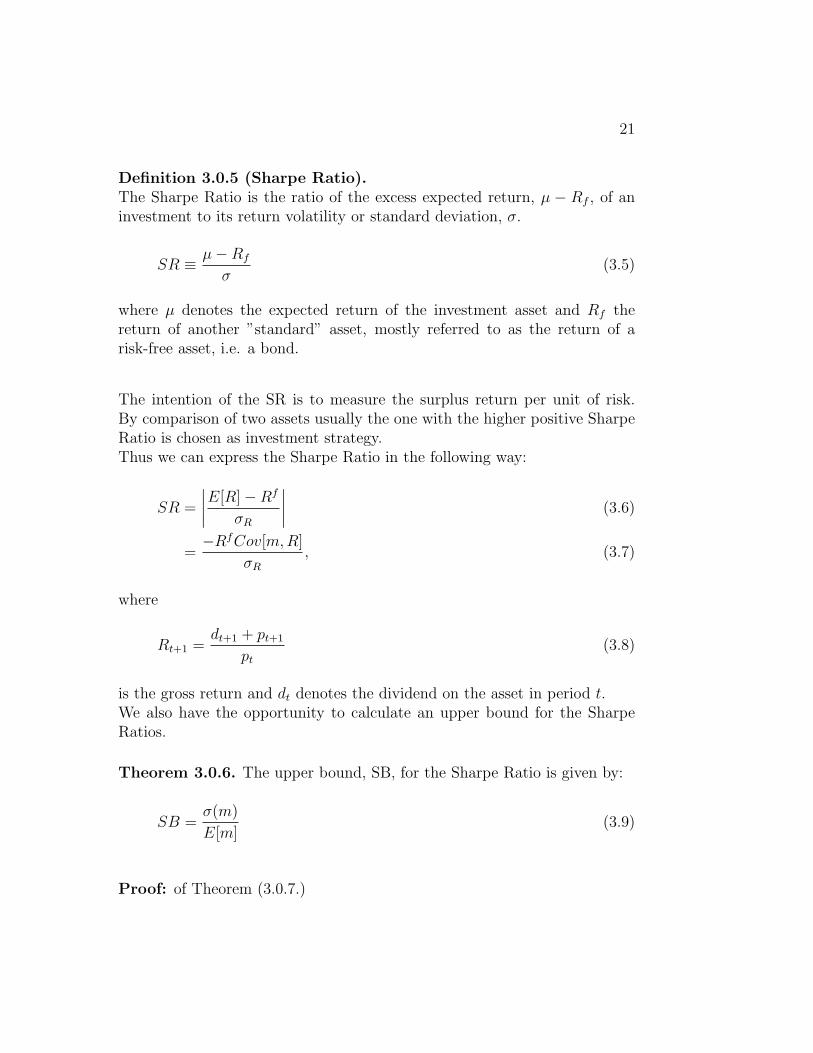
Definition 3.0.5 (Sharpe Ratio).The Sharpe Ratio is the ratio of the excess expected return, µ − Rf , of aninvestment to its return volatility or standard deviation, σ.
SR ≡ µ−Rf
σ(3.5)
where µ denotes the expected return of the investment asset and Rf thereturn of another ”standard” asset, mostly referred to as the return of arisk-free asset, i.e. a bond.
The intention of the SR is to measure the surplus return per unit of risk.By comparison of two assets usually the one with the higher positive SharpeRatio is chosen as investment strategy.Thus we can express the Sharpe Ratio in the following way:
SR =
∣∣∣∣E[R]−Rf
σR
∣∣∣∣ (3.6)
=−RfCov[m, R]
σR
, (3.7)
where
Rt+1 =dt+1 + pt+1
pt
(3.8)
is the gross return and dt denotes the dividend on the asset in period t.We also have the opportunity to calculate an upper bound for the SharpeRatios.
Theorem 3.0.6. The upper bound, SB, for the Sharpe Ratio is given by:
SB =σ(m)
E[m](3.9)
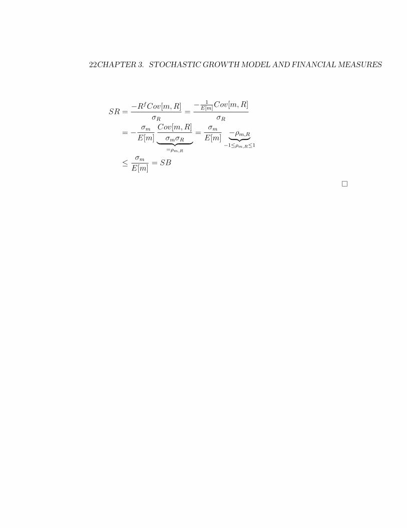
Proof: of Theorem (3.0.7.)
22CHAPTER 3. STOCHASTIC GROWTH MODEL AND FINANCIAL MEASURES
SR =−RfCov[m, R]
σR
=− 1
E[m]Cov[m,R]
σR
= − σm
E[m]
Cov[m, R]
σmσR︸ ︷︷ ︸=ρm,R
=σm
E[m]−ρm,R︸ ︷︷ ︸
−1≤ρm,R≤1
≤ σm
E[m]= SB

Chapter 4
Reference Model
We will now have a closer look at the most basic stochastic growth model,as in Grune and Semmler [7] in chapter 5. The general set-up as in Mirmanand Brock [2] was already introduced in chapter 2.
4.1 The Model
In our model we will now have log utility, i.e. u(ct) = ln u(ct), aggregate cap-ital stock and labour augmenting technology shocks. In detail, the problemset-up is as follows:
V (k, z) := maxct
E[∞∑
t=0
βt ln(ct)] (4.1)
subject to
kt+1 =ztAkαt − ct
ln zt+1=ρ ln zt + εt
=: ϕ((k, z), c, ε)
A, α and ρ are real constants and the εt are i.i.d. random variables with zeromean. For numerical reasons we substitute ln zt by yt. Important for the timeseries is the fact that εt is chosen as a Gaussian distributed random variablewith standard deviation σ = 0.008. The domain in which we will compute the
23

24 CHAPTER 4. REFERENCE MODEL
model, Ω = [0.1, 10]× [−0.32, 0.32], can be controlled invariant, that meansthere exists an optimal consumption path c such that ϕ((k, z), c, ε) ∈ Ω forany (k, z) ∈ Ω and for all ε. The difference between the model in Grune andSemmler, [7], p. 15 and this model is, that, since we do not work on grids, wedo not have to restrict ε on the interval [−0.032, 0.032], which is very handyfor the time series approach. The topic restriction will be discussed again inchapter 6, when the random variable approach is introduced.This model is equivalent to the stochastic growth model of chapter 2. thedifference is just, that in our model the discount factor is given by β insteadof δ, and we will give initial values for z and k instead an initial value fors = c0 + k0 as was in the Mirman and Brock,[2] set-up.
4.2 The Optimal Value and Control Function
An interesting feature of the value function (4.1) is that it can also be writtenas
V (k, z) = maxc
E[u(c(k, z)) + βV (ϕ((k, z), c(k, z), ε))] (4.2)
This is the Bellman equation. It reduces the multi-period optimization to atwo-stage problem, effectively. At first we maximize current utility by takinginto account that the choice ct affects future possibilities through kt+1. Then,in the future we also maximize so that our outcome can be summarizedby the expected discounted future value function. This insight in dynamicprogramming is referred to as the optimality principle, see Geraats, [5]
As mentioned above our model can be solved analytically for the policyfunction in feedback form. Thus a sequence of optimal consumption canbe derived and used for the numerical solution of the asset’s price and theSharpe Ratio.The following remark will give the optimal value and control function, seeGrune, [9].
Remark 4.2.1. V ∗(k, z) is the optimal value function for problem (4.1) givenby
V ∗(k, z) = B + C ln (k) + D ln(z)
4.2. THE OPTIMAL VALUE AND CONTROL FUNCTION 25
with
B =ln (1− αβ)A + αβ
1−αβln αβA
1− β,
C =α
1− αβ
and
D =1
(1− αβ)(1− ρβ)
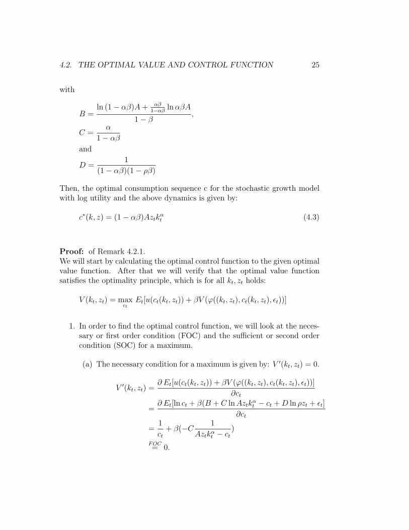
Then, the optimal consumption sequence c for the stochastic growth modelwith log utility and the above dynamics is given by:
c∗(k, z) = (1− αβ)Aztkαt (4.3)
Proof: of Remark 4.2.1.We will start by calculating the optimal control function to the given optimalvalue function. After that we will verify that the optimal value functionsatisfies the optimality principle, which is for all kt, zt holds:
V (kt, zt) = maxct
Et[u(ct(kt, zt)) + βV (ϕ((kt, zt), ct(kt, zt), εt))]
1. In order to find the optimal control function, we will look at the neces-sary or first order condition (FOC) and the sufficient or second ordercondition (SOC) for a maximum.
(a) The necessary condition for a maximum is given by: V ′(kt, zt) = 0.
V ′(kt, zt) =∂ Et[u(ct(kt, zt)) + βV (ϕ((kt, zt), ct(kt, zt), εt))]
∂ct
=∂ Et[ln ct + β(B + C ln Aztk
αt − ct + D ln ρzt + εt]
∂ct
=1
ct
+ β(−C1
Aztkαt − ct
)
FOC= 0.
26 CHAPTER 4. REFERENCE MODEL
⇒ Aztktα
ct
− 1− βC = 0
⇐⇒ Aztkαt
1 + βC= ct
with C = α1−αβ
⇒ (1− αβ)Aztkαt = c∗t .
(b) If c∗t maximizes V ∗ and V ∗ is twice differentiable, thenV ∗′′(kt, zt; c
∗t ) ≤ 0 has to hold. (SOC)
V ′′(kt, zt) =∂2 Et[u(ct(kt, zt)) + βV (ϕ((kt, zt), ct(kt, zt), εt))]
∂c2t
= Et[−1
c2t
− −βC(−1)
(Aztkαt − ct)2
]
with c∗t
⇒ Et[−1
((1− αβ)Aztkαt )2︸ ︷︷ ︸
>0
− βC
(αβAztkαt )2︸ ︷︷ ︸
>0
]
< 0.
2. c∗t is the optimal control function, which means that c∗t maximizesV ∗(kt, zt) at every point in time and for all (kt, zt).V ∗(kt, zt) = maxct Et[u(ct(kt, zt))+βV ∗(ϕ((kt, zt), ct(kt, zt), εt))] has tohold if V ∗ is the optimal value function.Thus it is sufficient to show that V ∗(kt, zt) satisfiesV ∗(kt, zt) = Et[u(c∗t (kt, zt)) + βV ∗(ϕ((kt, zt), c
∗t (kt, zt), εt))] in order to
prove that it is the optimal value function.
Let us now start by looking at the right side of the above formula andsubstituting ln zt by yt:
Et[V∗(ϕ((kt, yt), c
∗t (kt, yt), εt))]
= Et[B + C ln(eytAkαt − (1− αβ)Aeytkα
t )︸ ︷︷ ︸ln(αβA)+yt+α ln(kt)
+D (ρ yt + εt)]
4.2. THE OPTIMAL VALUE AND CONTROL FUNCTION 27
= B + C (ln(αβA) + yt + α ln(kt)) + D ρ yt + D Et[εt]︸ ︷︷ ︸=0
B,C,D=
ln((1−αβ)A)+ α1−αβ
ln(αβA)
1−β+ α(1−ρβ)+ρ
(1−αβ)(1−ρβ)yt
+ α2
1−αβln(kt)
⇒V ∗(kt, zt)= Et[u(ct(kt, zt)) + βV ∗(ϕ((kt, zt), c∗t (kt, zt), εt))]
= Et[ln((1− αβ)eyt Akα
t ) + βV ∗(ϕ((kt, zt), c∗t (kt, zt), εt))]
= ln((1− αβ)A)ytα ln(kt) + βEt[V∗(ϕ((kt, zt), c
∗t (kt, zt), εt))]
= ln((1− αβ)A)ytα ln(kt)
+βln((1−αβ)A) α
1−αβln(αβ)
1−β
+ α(1−ρβ)+ρ(1−αβ)(1−ρβ)
yt + α2
1−αβln(kt))
=ln((1− αβ)A) + αβ
1−αβln(αβA)
1− β︸ ︷︷ ︸=B
+(1− αβ + αβ)(1− ρβ) + ρβ
(1− αβ)(1− ρβ)︸ ︷︷ ︸=D
yt
+α
1− αβ︸ ︷︷ ︸C
ln(kt)
= B + C ln(kt) + Dyt
As we have seen in the last chapter m(ct, ct+1) = β u′(ct+1)u′(ct)
. For our optimalcontrol function c, m is given by:
m(ct, ct+1) = βct)
ct+1)(4.4)
The last thing we need before we can start calculating the Sharpe Ratios isthe price formula.
Remark 4.2.2. The price for a wealth portfolio with log utility is propor-
28 CHAPTER 4. REFERENCE MODEL
tional to consumption. In our case the formula is given by:
pt =β
1− β(1− αβ)Aztk
αt (4.5)
Proof: of Remark 4.2.2.We need to look at the present-value formula for the price of a wealth portfo-lio. In this context the wealth portfolio is a claim to all future consumption.We yield:
pt = Et
[∞∑
j=1
βj u′(ct+j)
u′(ct)ct+j
]
= Et
[∞∑
j=1
βj ct
ct+j
ct+j
]geometric series
=β
1− βct
We will need these formulas for both approaches to a solution of the maxi-mization problem.
4.3 The Dynamics in the Long Run
Figure 4.1 will give a rough impression of paths k to different start values ofk and z and along optimal trajectories. It can easily be seen that all trajec-tories oscillate around the point (k, ln z) ≈ (2, 0) in the long run.
In the next two chapters we will work through solutions of the problemof calculating the Sharpe Ratio by looking at the time series of the dynam-ics and as the second approach we will look at m(xt) as a random variable.In chapter 7 we will compare both attempts with each other and with theanalytical solution as can be found in Grune and Semmler, [7].

4.3. THE DYNAMICS IN THE LONG RUN 29
Figure 4.1: k-components of optimal trajectories for z(0) = −0.32, 0, 0.32

Chapter 5
Time Series Approach
In this chapter we will solve the problem of calculating the Sharpe Ratio asdescribed in the last chapter by modelling the time series of our dynamics,z and k. Both need to be modelled in order to find possible paths for con-sumption c. As we have already seen, all time series for the capital stock,k, independent of their initial values oscillate around some kind of ”equilib-rium” point. Because of that and the fact, that we are just interested in thelong time behaviour of our economy, it is enough to always model one pathinstead of several ones as it is usually done in Monte Carlo Simulations.
5.1 Random Number Generators
In our stochastic growth model the stochastic factor, ε, is said to be stan-dard normally distributed with zero mean and a standard deviation of 0.008.Therefore we will need a standard normally distributed random variable.Since every simulation of random variables is a deterministic operation thenumbers we generate are said to be pseudo random variables. Since there isno Pseudo Random Number Generator with that distribution implementedunder MATLAB, it is necessary to implement one. A way to do so was de-scribed in ”Finanzderivate mit MATLAB” by M. Gunther and A. Jungel,[10].The first step is to produce uniformly distributed pseudo random variables
30

5.1. RANDOM NUMBER GENERATORS 31
in the interval [0, 1],
Y ∼ U [0, 1],
which are transformed into normally distributed random numbers by usinga function h.
Z := h(Y ) ∼ N(0, 1)
Both terms were already defined in chapter 1. The exact implementation ofthe algorithms used in this chapter are in the appendix.
Step 1 The uniformly distributed random numbers are produced by laggedFibonacci-Generators based on Tausworth.
for i ≥ max µ, ν
Xi := (Xi−µ + Xi−ν) mod M,
Ui := Xi/M,
where X1, ..., Xµ,ν are generated by a standard MATLAB random num-ber generator.
Step 2 Uniformly distributed random numbers are transformed by the al-gorithm based on Box-Muller: Generate U1, U2 ∼ U [0, 1]. Then Z1 =√
(− 2 ln U1) cos(2πU2) and Z2 =√
(− 2 ln U1) sin(2πU2) are standardnormally distributed.
Step 3 Since we need random numbers that are normally distributed withzero mean and standard deviation of 0.008 we take the standard nor-mally distributed random numbers, Zi, i = 1..N generated in step 2and the transformation Xi = 0.008Zi, for all i. The Xi are N(0, 0.008).
The basis for step 2 is the following theorem:
Theorem 5.1.1. Let X be a random variable with probability density f ona set A = x ∈ (R) : f(x) > 0. The transformation h : A → B = h(A) beinvertible and the inverse h−1 be continuous. Then Y = h(X) has the densityfunction
y 7→ f(h−1(y))
∣∣∣∣det(dh−1
dy(y))
∣∣∣∣ , y ∈ B.

32 CHAPTER 5. TIME SERIES APPROACH
Proof: of Step 3.Let Y ∼ N(0, 1). Now, consider X = σY + µ.
Expected Value: E(X)(2.8)= σE(Y ) + µ = µ
Variance: V ar(X)(2.8)= σ2V ar(Y ) = σ2
Thus X ∼ N(µ, σ2), which means for our model that we have generated astochastic factor ε ∼ N(0, 0.0082).
5.2 Solving the model
As soon as we have generated our standard normally distributed pseudorandom variables εt we can model a path for the development of labour overtime.Remember the dynamics for z are given by: ln zt+1 = ρ ln zt + εt
For computational reasons, we will work with the logarithm at the latestpossible point during our analysis. Therefore we rewrite the equation bysubstituting ln z = y. We get:
yt+1 = ρyt + εt (5.1)
kt+1 = eytAkαt − ct (5.2)
Starting with modelling the path for y we get the path for z by taking zt = eyt
for t = 1 · · ·N . Figure 5.1 shows a possible outcome for both y and z for aninitial value y(0) = 0. See Appendix A.2 for the exact MATLAB code.
In the next step both path y and path c are modelled, since both aredependent of each other. As one can see in the formula for k, c is alreadyincluded, but is one time step aback. Thus, if k is computed on the interval[0, N ], then c will just be computed from 0 up to the point N − 1. Sincewe know the optimal control function to our particular stochastic growthproblem, we can calculate an initial value for c as long as we have choseninitial values for y and for z. Again the exact MATLAB code is given inAppendix A.2.. In figure 5.2 the initial values are k(0) = 0.1 and y(0) = 0.
From there it is easy to calculate the stochastic growth factor m. Remember

5.2. SOLVING THE MODEL 33
Figure 5.1: Paths for y and z
Figure 5.2: Path for capital k and consumption c

34 CHAPTER 5. TIME SERIES APPROACH
(4.4):
m(ct, ct+1) = βct
ct+1
.
One path for m(ct, ct+1) is given in Figure 5.3 for the usual initial values usedthroughout this chapter. Looking again at chapter 3, where the asset price
Figure 5.3: The stochastic discount factor m
characteristics in the context of a stochastic growth model were introduced,it can be seen, that we need the expected value and the standard deviationof m for computing the risk-free interest rate Rf , the Upper Bound SB andthe Sharpe Ratio SR, itself. See (3.3),(3.6),(3.7) and (3.9).If we choose initial values y(0) = 0, k(0) = 0.1 and a time horizon of N = 50
5.2. SOLVING THE MODEL 35
we get:
E[m] =1
N − 1
N−2∑t=0
m(ct, ct+1) = 0.9343 (5.3)
σm =
√√√√ 1
N − 1
N−2∑t=0
V ar[m(ct, ct+1)] = 0.0726 (5.4)
Rf =1
E[m]= 1.0704 (5.5)
SB =σm
E[m]= 0.0760. (5.6)
In the formula for the expected value for m, it is only divided by N-1, becausewe just have N values for c(xt). Since we use ct+1 for calculating m(ct, ct+1)we always look one consumption step ahead of time and therefore yield N−1values for m.
Consider the Sharpe Ratio as introduced in chapter 3. In order to computethe Sharpe Ratio we have to find the return path first. Therefore we have alook at at the price formula of this problem, which is given by (4.5).
pt =β
1− β(1− αβ)Aztk
αt
Figure 5.4 shows a price path to our model with initial values y(0) = 0and k(0) = 0.1. As soon as we have our prices to different points in timewe can calculate the return. Since the wealth portfolio is a claim to futureconsumption the dividend dt is given by consumption ct. Therefore the grossreturn function becomes:
Rt+1 =ct+1 + pt+1
pt
(5.7)
Figure 5.5 shows the path for the gross return for our consumption basedmodel with initial values as used above. Now, we can start to evaluate theSharpe Ratio for our model. Starting from R, we are able to compute theexpectation of R over time, the covariance of gross return R and stochastic

36 CHAPTER 5. TIME SERIES APPROACH
Figure 5.4: The price p
Figure 5.5: The gross return R

5.3. SHARPE RATIOS SUBJECT TO INITIAL VALUES 37
growth model m and finally the Sharpe Ratio.
E[R] =1
N − 1
N−2∑t=0
Rt = 1.0815 (5.8)
σR =
√√√√ 1
N − 1
N−2∑t=0
V ar[Rt] = 0.1473 (5.9)
Cov[R,m] =1
N − 1
N−2∑t=0
Cov[Rt, mt] = −0.0103 (5.10)
SR =−RfCov[m, R]
σ[R]= 0.0751. (5.11)
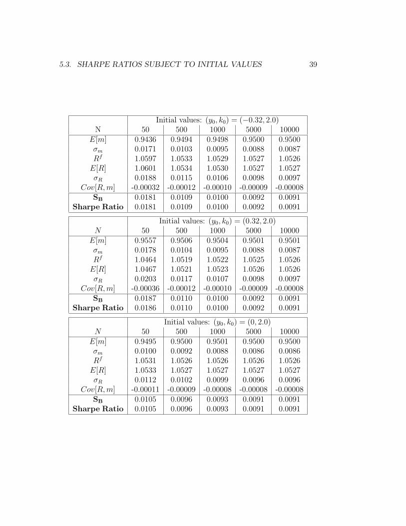
5.3 Sharpe Ratios subject to initial values
In this chapter we will give solutions for the Sharpe Ratio and relevant assetprice characteristics subject to different initial values in Table 5.1. Rememberthe domain in which we compute the model is Ω = [0.1, 10]×[−0.32, 0.32] andthat the paths for y and k oscillate approximately around some ”equilibrium”point (0, 2) at a pretty early point in time. We have seen in Figure 4.1 thatit already starts to oscillate when a time horizon of just N = 50 is chosen.Nonetheless even for any pair of initial values with k = 2 a time horizonof N = 10000 is needed to get to a final value for the Sharpe Ratio. Forany other pair of initial values the maximum time horizon is chosen to beN = 50000, see Table 5.1..The MATLAB codes generating these results aregiven in appendix (A.2)

38 CHAPTER 5. TIME SERIES APPROACH
We find that the Sharpe Ratios differ from the Sharpe Ration given by Gruneand Semmler, [7], p.16, that is 0.007999.
Before we analyse the model for reasons for this difference in chapter 7, wewill have a look at the random variable approach in chapter 6.
5.3. SHARPE RATIOS SUBJECT TO INITIAL VALUES 39
Initial values: (y0, k0) = (−0.32, 2.0)N 50 500 1000 5000 10000
E[m] 0.9436 0.9494 0.9498 0.9500 0.9500σm 0.0171 0.0103 0.0095 0.0088 0.0087Rf 1.0597 1.0533 1.0529 1.0527 1.0526
E[R] 1.0601 1.0534 1.0530 1.0527 1.0527σR 0.0188 0.0115 0.0106 0.0098 0.0097
Cov[R,m] -0.00032 -0.00012 -0.00010 -0.00009 -0.00008SB 0.0181 0.0109 0.0100 0.0092 0.0091
Sharpe Ratio 0.0181 0.0109 0.0100 0.0092 0.0091
Initial values: (y0, k0) = (0.32, 2.0)N 50 500 1000 5000 10000
E[m] 0.9557 0.9506 0.9504 0.9501 0.9501σm 0.0178 0.0104 0.0095 0.0088 0.0087Rf 1.0464 1.0519 1.0522 1.0525 1.0526
E[R] 1.0467 1.0521 1.0523 1.0526 1.0526σR 0.0203 0.0117 0.0107 0.0098 0.0097
Cov[R,m] -0.00036 -0.00012 -0.00010 -0.00009 -0.00008SB 0.0187 0.0110 0.0100 0.0092 0.0091
Sharpe Ratio 0.0186 0.0110 0.0100 0.0092 0.0091
Initial values: (y0, k0) = (0, 2.0)N 50 500 1000 5000 10000
E[m] 0.9495 0.9500 0.9501 0.9500 0.9500σm 0.0100 0.0092 0.0088 0.0086 0.0086Rf 1.0531 1.0526 1.0526 1.0526 1.0526
E[R] 1.0533 1.0527 1.0527 1.0527 1.0527σR 0.0112 0.0102 0.0099 0.0096 0.0096
Cov[R,m] -0.00011 -0.00009 -0.00008 -0.00008 -0.00008SB 0.0105 0.0096 0.0093 0.0091 0.0091
Sharpe Ratio 0.0105 0.0096 0.0093 0.0091 0.0091

40 CHAPTER 5. TIME SERIES APPROACH
Initial values: (y0, k0) = (−0.32, 9.0)N 50 500 1000 5000 10000 50000
E[m] 0.9552 0.9506 0.9503 0.9501 0.9501 0.9500σm 0.0711 0.0241 0.0181 0.0111 0.0099 0.0088Rf 1.0468 1.0520 1.0523 1.0525 1.0526 1.0526
E[R] 1.0509 1.0525 1.0525 1.0527 1.0527 1.0527σR 0.0551 0.0199 0.0156 0.0110 0.0103 0.0097
Cov[R,m] -0.0039 -0.00047 -0.00028 -0.00012 -0.00010 -0.00008SB 0.0744 0.0254 0.0190 0.0117 0.0105 0.0093
Sharpe Ratio 0.0739 0.0250 0.0187 0.0115 0.0103 0.0092
Initial values: (y0, k0) = (0.32, 9.0)N 50 500 1000 5000 10000 50000
E[m] 0.9662 0.9517 0.9509 0.9502 0.9501 0.9501σm 0.0437 0.0170 0.0135 0.0098 0.0092 0.0086Rf 1.0349 1.0508 1.0516 1.0524 1.0525 1.0526
E[R] 1.0367 1.0511 1.0518 1.0525 1.0526 1.0527σR 0.0395 0.0165 0.0135 0.0105 0.0100 0.0096
Cov[R,m] -0.0017 -0.00028 -0.00018 -0.00011 -0.00009 -0.00008SB 0.0452 0.0178 0.0142 0.0103 0.0097 0.0091
Sharpe Ratio 0.0450 0.0177 0.0140 0.0102 0.0096 0.0091
Initial values: (y0, k0) = (0, 9.0)N 50 500 1000 5000 10000 50000
E[m] 0.9606 0.9511 0.9506 0.9501 0.9501 0.9501σm 0.0558 0.0199 0.0153 0.0103 0.0095 0.0087Rf 1.0410 1.0514 1.0520 1.0525 1.0525 1.0526
E[R] 1.0437 1.0518 1.0522 1.0526 1.0526 1.0527σR 0.0463 0.0177 0.0142 0.0107 0.0101 0.0096
Cov[R,m] -0.0026 -0.00035 -0.00021 -0.00011 -0.00010 -0.00008SB 0.0581 0.0209 0.0161 0.0108 0.0100 0.0092
Sharpe Ratio 0.0578 0.0207 0.0159 0.0107 0.0099 0.0091

5.3. SHARPE RATIOS SUBJECT TO INITIAL VALUES 41
Initial values: (y0, k0) = (−0.32, 0.1)N 50 500 1000 5000 10000 50000
E[m] 0.9276 0.9478 0.9490 0.9498 0.9499 0.9500σm 0.0660 0.0236 0.0178 0.0110 0.0099 0.0088Rf 1.0780 1.0550 1.0538 1.0528 1.0527 1.0526
E[R] 1.0869 1.0561 1.0543 1.0530 1.0528 1.0527σR 0.1262 0.0423 0.0307 0.0162 0.0133 0.0104
Cov[R,m] -0.0082 -0.00097 -0.00053 -0.00017 -0.00013 -0.00009SB 0.0712 0.0249 0.0187 0.0116 0.0104 0.0093
Sharpe Ratio 0.0703 0.0243 0.0182 0.0112 0.0100 0.0091
Initial values: (y0, k0) = (0.32, 0.1)N 50 500 1000 5000 10000 50000
E[m] 0.9140 0.9492 0.9496 0.9500 0.9500 0.9500σm 0.0769 0.0259 0.0193 0.0115 0.0102 0.0089Rf 1.0627 1.0536 1.0530 1.0527 1.0526 1.0526
E[R] 1.0765 1.0550 1.0538 1.0529 1.0528 1.0527σR 0.1710 0.0554 0.0398 0.0197 0.0155 0.0110
Cov[R,m] -0.00130 -0.0014 -0.00074 -0.00021 -0.00015 -0.00009SB 0.0817 0.0273 0.0203 0.0122 0.0107 0.0093
Sharpe Ratio 0.0805 0.0266 0.0196 0.0114 0.0100 0.0090
Initial values: (y0, k0) = (0, 0.1)N 50 500 1000 5000 10000 50000
E[m] 0.9342 0.09485 0.9493 0.9499 0.9500 0.9500σm 0.0710 0.0425 0.0184 0.0112 0.0100 0.0088Rf 1.0704 1.0543 1.0534 1.0528 1.0527 1.0526
E[R] 1.0815 1.0555 1.0541 1.0530 1.0528 1.0527σR 0.1473 0.0483 0.0349 0.0178 0.0143 0.0106
Cov[R,m] -0.0103 -0.0012 -0.00062 -0.00019 -0.00014 -0.00009SB 0.0760 0.0258 0.0193 0.0118 0.0105 0.0093
Sharpe Ratio 0.0751 0.0252 0.0187 0.0112 0.0100 0.0091
Table 5.1: Sharpe Ratios depending on initaial values

Chapter 6
Random Variable Approach
This chapter covers the random variable approach to our stochastic growthmodel. First, note, that all MATLAB codes used throughout this chaptercan be found in appendix A.3.
6.1 Restrictions on ε
As one could see in chapter 4 the stochastic discount factor is given by:
m(ct, ct+1) = βct
ct+1
We will know look at m as a function of our random variable ε, which goesinto the function via z and therefore c. Substituting the control function forc into the formula for m and just looking one step ahead from the initialvalues gives us:
m(k, y) =βey0k0
α
eρy0+εαβAey0k0α (6.1)
Again we have to find the Expected Value of m and and several other char-acteristics in order to calculate the Upper Bound and the Sharpe Ratio.
If we want to calculate the expected value of our random variable m, we have
42

6.1. RESTRICTIONS ON ε 43
Figure 6.1: density function of ε in [−0.5, 0.5]
to use the density function of ε. Since ε ∼ N(0, 0.008) the density functionis:
∼f (ε) =
1√2πσ2
e−12
ε2
0.0082 (6.2)
Because of the fact that we work with MATLAB and that uses numericalmethods for the calculation of integrals, we have to restrict the interval for ε.Figure 6.1 shows the density function. Obviously the numbers in the tail ofthe figure are very close to zero. A cutout of the right tail is given in Figure6.2. This figure gives us the impression that all values outside the interval[−0.05, 0.05] are approximately 0. In order to ceck that impression we alsocalculate the density function in the interval [−0.05, 0.05] and look at thosetails.
Thus we see that using the interval [−0.032, 0.032] is sufficient for ourcalculation. We will use this interval, since it was also used in Grune and
Figure 6.2: density function of ε in [−0.05, 0.05]
44 CHAPTER 6. RANDOM VARIABLE APPROACH
Semmler, [7], p. 15. If we broaden the interval the values we get for theSharpe Ratio and other characteristics do not change any more.
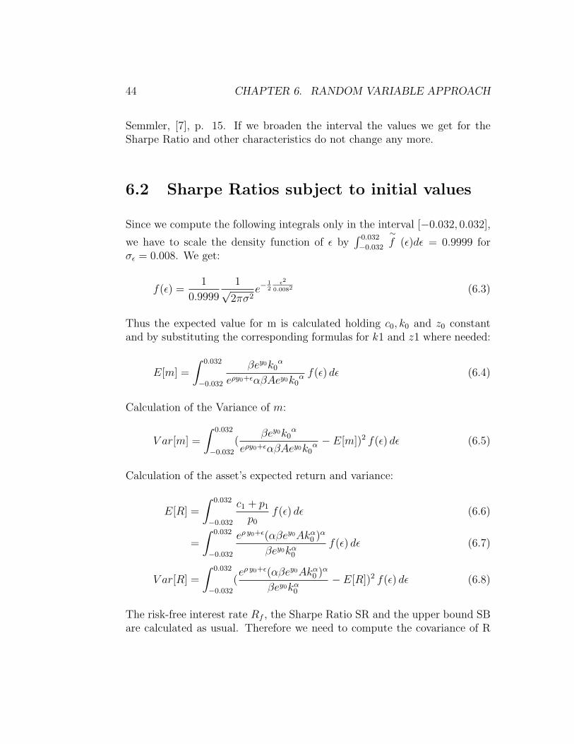
6.2 Sharpe Ratios subject to initial values
Since we compute the following integrals only in the interval [−0.032, 0.032],
we have to scale the density function of ε by∫ 0.032
−0.032
∼f (ε)dε = 0.9999 for
σε = 0.008. We get:
f(ε) =1
0.9999
1√2πσ2
e−12
ε2
0.0082 (6.3)
Thus the expected value for m is calculated holding c0, k0 and z0 constantand by substituting the corresponding formulas for k1 and z1 where needed:
E[m] =
∫ 0.032
−0.032
βey0k0α
eρy0+εαβAey0k0α f(ε) dε (6.4)
Calculation of the Variance of m:
V ar[m] =
∫ 0.032
−0.032
(βey0k0
α
eρy0+εαβAey0k0α − E[m])2 f(ε) dε (6.5)
Calculation of the asset’s expected return and variance:
E[R] =
∫ 0.032
−0.032
c1 + p1
p0
f(ε) dε (6.6)
=
∫ 0.032
−0.032
eρ y0+ε(αβey0Akα0 )α
βey0kα0
f(ε) dε (6.7)
V ar[R] =
∫ 0.032
−0.032
(eρ y0+ε(αβey0Akα
0 )α
βey0kα0
− E[R])2 f(ε) dε (6.8)
The risk-free interest rate Rf , the Sharpe Ratio SR and the upper bound SBare calculated as usual. Therefore we need to compute the covariance of R

6.2. SHARPE RATIOS SUBJECT TO INITIAL VALUES 45
and m, as well.
Cov[R,m] =
∫ 0.032
−0.032
(c1 + p1
p0
− E[R])(βc0
c1
− E[m]) f(ε) dε (6.9)
=
∫ 0.032
−0.032
(eρ y0+ε(αβey0Akα
0 )α
βey0kα0
− E[R]) (6.10)
· ( βey0k0α
eρy0+εαβAey0k0α − E[m]) f(ε) dε (6.11)
Table 6.1 shows the characteristics depending on various initial values. TheMATLAB codes generating these results are given in appendix (A.2).
In the Table all numbers are only calculated up to the fourth decimal digit.The more exact Sharpe Ratio is 0.00799533412689, which fits nicely with theresult as can be found in Grune and Semmler, [7], p.16, that is 0.007999.

46 CHAPTER 6. RANDOM VARIABLE APPROACH
Initial values: k(0) = 0.1y(0) = 0 y(0) = −0.32 y(0) = 0.32
E[m] 0.4815 0.5199 0.4459σm 0.0038 0.0042 0.0036Rf 2.0770 1.9235 2.2428
E[R] 2.0772 1.9236 2.2430σR 0.0166 0.0154 0.0179
Cov[R,m] -0.00006 -0.00006 -0.00006SB 0.0080 0.0080 0.0080SR 0.0080 0.0080 0.0080
Initial values: k(0) = 9.0y(0) = 0 y(0) = −0.32 y(0) = 0.32
E[m] 1.3216 1.4271 1.2239σm 0.0106 0.0114 0.0098Rf 0.7567 0.7007 0.8171
E[R] 0.7567 0.7008 0.8171σR 0.0061 0.0056 0.0065
Cov[R,m] -0.00006 -0.00006 -0.00006SB 0.0080 0.0080 0.0080SR 0.0080 0.0080 0.0080
Initial values: k(0) = 2.0y(0) = 0 y(0) = −0.32 y(0) = 0.32
E[m] 0.9430 1.0183 0.8733σm 0.0075 0.0081 0.0070Rf 1.0604 0.9821 1.1451
E[R] 1.0605 0.9821 1.1452σR 0.0085 0.0079 0.0092
Cov[R,m] -0.00006 -0.00006 -0.00006SB 0.0080 0.0080 0.0080SR 0.0080 0.0080 0.0080
Table 6.1: Sharpe Ratios depending on initial values
Chapter 7
Comparison
As one can see by comparing the results of chapter 5 and chapter 6, Table5.1 and Table 6.1, the results differ rather a lot. At first we have to note thatthe only results we can really compare and which we hoped to be equal arethe Sharpe Ratio and the upper bound. We do now have to admit that bothapproaches have rather different outcomes.Consider the initial values (y0, k0) = (0, 0.1). Then the result for examplefor E[m] is 0.4815 when using the random variable approach and the resultis 0.9500 for the time series with N = 10000. It is important to mentionthat we cannot compare those results with each other since in the time seriesapproach we middle over a lot of results in the long run, that oscillate at apretty early point in time approximately around (y, k) ∼ (0, 2). Thus we cancompare the outcome of E[m] from the time series only with the outcome ofthe random variable for initial values (y0, k0) = (0, 2). Same holds for Rf
and E[R].Nonetheless the results obviously do not fit, therefore we need to take amore detailed look at the programmes and the differences between both ap-proaches. We want to begin this analysis by checking the time series pro-gramme for correctness. After that we will have a look at the correlationsbetween the random variables in both programmes.
47

48 CHAPTER 7. COMPARISON
7.1 Programme Check
We will now verify all programmes needed for the time series approach. Thecodes are given in Appendix (A.2).At first we want to check if the equations for the time series for y, k and cwork properly. One way to do so is to rewrite some of the equations. Assumethat we just generate N = 10000 results for y1, k1 and c1, i.e. we look atsample data just one time step ahead from the initial values. According tothe central limit theorem (2.1.18), averaging over these values should give usapproximately the same values for y, k and c as we would get by using therandom variable approach, which works by finding the expected value in onetime step. The Matlab code for simulating the sample datas are given in theprogramme SR control, (A.4)In order to generate the sample data we leave the programmes RWfibonacci.mand boxmuller.m the way they are, because we still need those N(0, 0.0082)distributed pseudo random variables ε. But we will change the routine inRefz, since we do not need a path over time but 10.000 results for the firsttime step. Thus we drop the time subscript t and use the subscript j to denotethe ”j-th sample data”. We rewrite the equation for yj+1 in the following way:
yj+1 = ρy0 + εj (7.1)
Note, that the parameter t is not a time subscript any more, but rather anindex denoting the number of an element of the sample data.After having generated the sample data for y, we will now have a closer lookat the formulas for k and c. Remember the original formulas:
kj+1 = eyjAkjα − cj
cj = (1− αβ)Aeyjkαj
For our problem those formulas become:
kj+1 = ey0Ak0α − c0 (7.2)
cj+1 = (1− αβ)Aeyjkα1 (7.3)
Note that the randomness just comes into the formula for cj+1 by yj, becausefor the calculation of kj+1 all parameters and initial values are fix. Thus wewill not have to calculate sample data for k. The sample data for cj+1 are
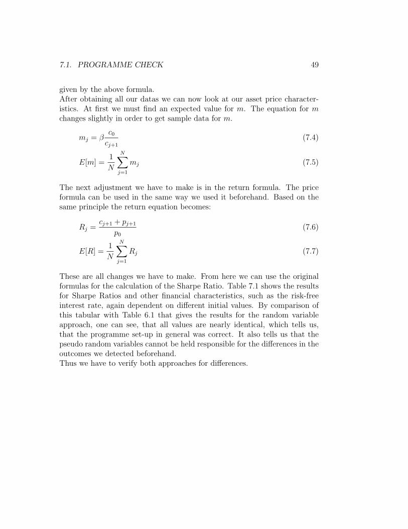
7.1. PROGRAMME CHECK 49
given by the above formula.After obtaining all our datas we can now look at our asset price character-istics. At first we must find an expected value for m. The equation for mchanges slightly in order to get sample data for m.
mj = βc0
cj+1
(7.4)
E[m] =1
N
N∑j=1
mj (7.5)
The next adjustment we have to make is in the return formula. The priceformula can be used in the same way we used it beforehand. Based on thesame principle the return equation becomes:
Rj =cj+1 + pj+1
p0
(7.6)
E[R] =1
N
N∑j=1
Rj (7.7)
These are all changes we have to make. From here we can use the originalformulas for the calculation of the Sharpe Ratio. Table 7.1 shows the resultsfor Sharpe Ratios and other financial characteristics, such as the risk-freeinterest rate, again dependent on different initial values. By comparison ofthis tabular with Table 6.1 that gives the results for the random variableapproach, one can see, that all values are nearly identical, which tells us,that the programme set-up in general was correct. It also tells us that thepseudo random variables cannot be held responsible for the differences in theoutcomes we detected beforehand.Thus we have to verify both approaches for differences.
50 CHAPTER 7. COMPARISON
Initial values: k(0) = 0.1y(0) = 0 y(0) = −0.32 y(0) = 0.32
E[m] 0.4814 0.5198 0.4458Rf 2.0772 1.9237 2.2430
E[R] 2.0774 1.238 2.2432SB 0.0080 0.0080 0.0080SR 0.0080 0.0080 0.0080
Initial values: k(0) = 9.0y(0) = 0 y(0) = −0.32 y(0) = 0.32
E[m] 1.3214 1.4269 1.2238Rf 0.7567 0.7008 0.8172
E[R] 0.7568 0.7008 0.8172SB 0.0080 0.0080 0.0080SR 0.0080 0.0080 0.0080
Initial values: k(0) = 2.0y(0) = 0 y(0) = −0.32 y(0) = 0.32
E[m] 0.9429 1.0182 0.8732Rf 1.0606 0.9821 1.1452
E[R] 1.0606 0.9822 1.1453SB 0.0080 0.0080 0.0080SR 0.0080 0.0080 0.0080
Table 7.1: Sharpe Ratios as an outcome of the control programme SR control
7.2 Correlations
The first thing we will do in this analysis is looking at the correlations be-tween the random variables and compare the results of both programmes. Inthis context the correlation coefficient indicates the strength and direction ofa linear relationship between two random variables. Thus correlation refersto the departure of two variables from independence. As one can easily seeby looking at the formula for consumption there is an interdependence ofy, kα and c. The bivariate plot given in Figure 7.1 shows the linear depen-dence of z and c. If one tries to fit a single straight line through the dots itwould have a positive slope. Thus we would also expect a positive relation-ship between those parameters. The correlation coefficient ρX,Y between two
7.2. CORRELATIONS 51
Figure 7.1: point pairs (z,c)
random variables was already defined in chapter 2.1 in definition 2.1.10. Wecan use this formula for the random variable approach. For the time seriesmodel the formula becomes:
ρz,c =1N
∑N−1t=0 ((zt − E[z])(ct − E[c]))√
1N
∑N−1t=0 ((zt − E[z])2
√1N
∑N−1t=0 ((ct − E[c])2
(7.8)
This equation obviously holds for all other time series as well. Table 7.2shows correlations in the time series model.
Let us now look at the correlations in the random variable model. Noteagain, that this approach only looks one time step ahead from the initialvalues when calculating the expectations, variances and covariances. It justintegrates by using the density function of εRemember the formula for k1.
k1 = ey0Ak0α − c0
It is obvious that there is no stochastic influence. All values that are neededfor its calculation are initial values. Thus the expected value E[k1] is equal
52 CHAPTER 7. COMPARISON
Initial values: k(0) = 0.1Cor[·, ·] y(0) = 0 y(0) = −0.32 y(0) = 0.32
[z, c] 0.9608 0.9832 0.9226[z, p] 0.9608 0.9832 0.9226[z, k] 0.8309 0.8918 0.7476[kα, c] 0.8894 0.9126 0.8682
Initial values: k(0) = 9.0Cor[·, ·] y(0) = 0 y(0) = −0.32 y(0) = 0.32
[z, c] 0.9634 0.9634 0.9664[z, p] 0.9634 0.9634 0.9664[z, k] 0.5845 0.5023 0.7456[kα, c] 0.8922 0.8379 0.9549
Initial values: k(0) = 2.0Cor[·, ·] y(0) = 0 y(0) = −0.32 y(0) = 0.32
[z, c] 0.9882 0.9886 0.9871[z, p] 0.9882 0.9886 0.9871[z, k] 0.8940 0.8973 0.8873[kα, c] 0.9518 0.9527 0.9487
Table 7.2: Correlations depending on initial values
to k1 itself, which means that its variance is 0. This in turn does not allowus to calculate the correlations between k and other variables, because wewould have to divide by zero. Whenever it is not possible to compute thecorrelation we will look at the covariance, since it already tells us if there isany kind of relationship between those variables.Since the degree of the relationship between all parameters does not changewith the initial values, Table 7.3 shows all correlations and covariances thatturn up in this model.
As we have already expected by looking at the random variable model set-up,there is no linear relationship in the stochastic sense of k and z, and kα andc. This is the main difference between both models, because for every pairof initial values there is always a positive linear relationship between thosevariables in the time series approach. At a closer look one even finds that inevery case, there is not only a relationship but also a strong one. Hence theresults for the Sharpe Ratio differ between both programmes.

7.3. σε AND MODEL OUTCOMES 53
Cor[·, ·] (y0, k0)[z, c] 1.0000[z, p] 1.0000
Cov[·, ·][z, k] 0[kα, c] 0
Table 7.3: Correlations and Covariances in the RV model
Considering that the influences vary that much between those models it isremarkable that the Sharpe Ratios are still quite close to each other. Thesmall variance of ε might account for this fact.
7.3 σε and Model Outcomes
In order to figure out what impact the chosen variance of ε does have onboth models and especially on the different outcomes we will now vary thevariance of ε in both programmes. Before we can calculate the Sharpe Ratioswe have to figure out the interval for the random variable approach. Figure7.2 shows the density function, when σε = 0.01. Thus we take the interval[−0.05, 0.05] for all calculations in the random variable approach.The following Table 7.4 shows the Sharpe Ratio and other characteristics,when ε ∼ N(0, 0.01) and the time horizon N in the time series approach isset to 50000.
Figure 7.2: density function of ε in [−0.5, 0.5], σε = 0.01

54 CHAPTER 7. COMPARISON
Initial Values(0, 2) (−0.32, 2) (0.32, 2)
RV TS RV TS RV TSE[m] 0.9430 0.9501 1.0183 0.9501 0.8733 0.9501Rf 1.0604 1.0526 0.9820 1.0526 1.1451 1.0526
E[R] 1.0605 1.0527 0.9821 1.0527 1.1452 1.0527Cov[R,m] -0.00010 -0.00013 -0.00010 -0.00013 -0.00010 -0.00013
SB 0.0100 0.0112 0.0100 0.0112 0.0100 0.0115SR cov 0.0100 0.0112 0.0100 0.0112 0.0100 0.0113
SR stand 0.0099 0.0112 0.0099 0.0112 0.0099 0.0113
Initial Values(0, 0.1) (0, 9) (−0.32, 9)
RV TS RV TS RV TSE[m] 0.4815 0.9500 1.3216 0.9501 1.4271 0.9501Rf 2.0770 1.0526 0.7567 1.0526 0.7007 1.0526
E[R] 2.0772 1.0527 0.7567 1.0527 0.7008 1.0527Cov[R,m] -0.00010 -0.00013 -0.00010 -0.00013 -0.00010 -0.00013
SB 0.0100 0.0115 0.0100 0.0114 0.0100 0.0114SR cov 0.0100 0.0113 0.0100 0.0113 0.0100 0.0114
SR stand 0.0099 0.0113 0.0099 0.0113 0.0099 0.0114
Table 7.4: Results for the Sharpe Ratio, σε = 0.01, N = 50000, ε ∈[−0.05, 0.05]
7.3. σε AND MODEL OUTCOMES 55
We notice that the results for both approaches are different to the results wefound in chapter 5 and 6 in Table 5.1 and 6.1. For both models the SharpeRatios are higher. Thus changing the variance to a higher level seems to resultin higher Sharpe Ratios. Looking at values in Table 7.4 more thoroughly wealso find that that all characteristics, except the upper bound and the SharpeRatio, are equal to the numbers we found in chapter 5 and 6. That means thereason for the different results can only be found in the standard deviationsof R and m. Consider for example the initial values (y0, k0) = (0, 2). Withσε = 0.008 we find σm = 0.0085 and σR = 0.0095 and with σε = 0.01 we findσm = 0.0106 and σR = 0.0119. Looking at the formulas (3.6),(3.7) and (3.9).we can account the change in the standard deviations for the change in theresults for the upper bound and the Sharpe Ratio.
In order to analyse the impact of the standard deviation σε on the SharpeRatios thoroughly more results are needed. Table 7.5 shows the results fordifferent standard deviations.
σε = 0.008ε ∈ [−0.032, 0.032]
RV TSE[m] 0.9430 0.9500Rf 1.0604 1.0526
E[R] 1.0605 1.0527SB 0.0080 0.0091SR 0.0080 0.0091
σε = 0.01ε ∈ [−0.05, 0.05]
RV TSE[m] 0.9430 0.9501Rf 1.0604 1.0526
E[R] 1.0605 1.0527SB 0.0100 0.0112SR 0.0099 0.0112

56 CHAPTER 7. COMPARISON
σε = 0.05ε ∈ [−0.25, 0.25]
RV TSE[m] 0.9441 0.9515Rf 1.0592 1.0510
E[R] 1.0618 1.0543SB 0.0500 0.0550SR 0.0499 0.0548
σε = 0.10ε ∈ [−0.45, 0.45]
RV TSE[m] 0.9477 0.9559Rf 1.0552 1.0462
E[R] 1.0658 1.0595SB 0.1002 0.1076SR 0.0992 0.1064
σε = 0.5ε ∈ [−2.5, 2.5]RV TS
E[m] 1.0685 1.0880Rf 0.9359 0.9191
E[R] 1.2017 1.2660SB 0.5329 0.4724SR 0.4151 0.3619
σε = 0.05ε ∈ [−5, 5]
RV TSE[m] 1.5546 1.5242Rf 0.6432 0.6561
E[R] 1.7484 2.3957SB 1.3095 0.8752SR 0.4827 0.3428
Table 7.5: Sharpe Ratios depending on σε, N = 50000, (y0, k0) = (0, 2)
So far, we are not able to compare the results with each other. Rememberthat we want to find out what impact has the standard deviation of ε on thedifference between the results for the Sharpe Ratios in both approaches. Wewill therefore look at the outcome ratios.
σε Ratio SRRVSRT S
0.008 0.87910.01 0.88390.05 0.50300.1 0.93230.5 1.14701 1.4081
Table 7.6: Sharpe Ratio ratios
For the first four ratios we get the impression that the higher we choosethe standard deviation for ε the closer the outcomes get to each other. The

7.3. σε AND MODEL OUTCOMES 57
smaller Sharpe Ratio of the random variable approach seems to react strongeron the higher standard deviation than the Sharpe Ratio of the random vari-able model. But as soon as we choose σε to be ”really” high we observe thatthe gap between the outcome of the time series approach and of the randomvariable becomes larger again and finally percentage wise is even larger thanit was at the beginning. Thus for high standard deviations the impact of σε isstronger on the time series approach than on the random variable approach.

Chapter 8
Asset Pricing with LossAversion
Since reality shows that consumption based models do not fit financial marketcharacteristics to time series data, in this chapter we will adjust our stochasticgrowth model for loss aversion. The main idea behind asset pricing modelswith loss aversion is, that someone who has experienced much losses on riskyassets in his past, will become even more careful with handling risky assetsin the future than he has already been beforehand. Thus we will now lookat a model taking one’s past experiences into consideration. The model weintroduce in this chapter is based on the paper by Grune and Semmler, [8].As for the basic consumption based model they used the stoachstic dynamicprogramming approach to solve for Sharpe Ratios.
8.1 Our Reference Model and Loss Aversion
Look back at the model set-up of our reference stochastic growth in chapter4. We will now adjust that model for the loss aversion. Thus, in this chapterwe want to maximize over
Et[∞∑
t=0
(βtu(ct) + btβt+1ν(Xt+1, St, rt))] (8.1)
58
8.1. OUR REFERENCE MODEL AND LOSS AVERSION 59
u(ct): denotes the utility over consumption. As usual we takeu(c) = ln c.β: is again the discount factorXt+1: is the change of wealthSt: the value of the agent’s risky assetsrt: a variable, measuring the agent’s gains or losses prior to periodt, denoted as a fraction of St. The economic interpretation of zt isthat it expresses the way of how the agent has experienced gainsor losses in the past affecting his or her willingness to take risks.Rt: is again the return on the risky assetRf : is still the risk-free interest rate as the case may be the returnon a risk-free asset.
More precisely we have:
1. The change in wealth is calculated as
Xt+1 = StRt − StRf (8.2)
The difference Rf −Rt can be positive, zero or negative.
2. Although rt can be greater, equal or smaller than one, with rt = 1 andthus with
ν(Xt+1, St, 1) =
Xt+1 for Xt+1 ≥ 0
λXt+1 for Xt+1 < 0.(8.3)
λ > 1 defined as follows:
λ(zt) = λ + k(rt − 1), (8.4)
k > 0. This models the fact that a loss is more severe than a gain. Forrt+1 we have:
rt+1 = ηztR
Rt+1
+ (1− η), (8.5)
η ∈ [0, 1] and R fixed, denoting the long time average of the risk-freeinterest rate.

60 CHAPTER 8. ASSET PRICING WITH LOSS AVERSION
3. The last parameter we have to discuss is bt, which is related to aggregateconsumption
∼ct in the following way:
bt = b0∼ct
−1, (8.6)
∼ct will be specified so as to hold the price-dividend ratio and the riskyasset premium stationary. One important paramter is b0, which pointsthe relevance of financial wealth on utility gains or losses relative toconsumption out. With b0 = 0 we obtain the usual consumption basedmodel.
This is our reference model adjusted for loss aversion. Now, we have to takea closer look at the formulas that we need for the calculation of the assetprice characteristics.
8.2 Loss Aversion and Financial Measures
Since our maximization problem changed due to the adjustment for riskaversion, we would also expect our formulas to change at least slightly. Sincethe utility function remains unchanged, the stochastic discount factor m forthe risk free interest rate does not change. We still have:
mf,t+1 = β
∼ct∼
ct+1
Thus Rf remains 1E[m]
. The first considerable change can be found in acharacterization for the risky asset. Remember in the consumption basedmodel we had E[mR] = 1 for the same reason that E[mRf ] = 1, see chapter3 (3.3). Now, we have:
1 = βEt[Rt+1
∼ct∼
ct+1
]︸ ︷︷ ︸=Et[mf,t+1Rt+1]
+b0βEt[∧ν (Rt+1, rt)] (8.7)
8.3. SOLUTION 61
with
∧ν (Rt+1, rt) =
Rt+1 −Rft , Rt+1 ≥ rtR
ft and rt ≤ 1
(rt − 1)Rft + λ(Rt+1 − rtR
ft ), Rt+1 < rtR
ft and rt ≤ 1
Rt+1 −Rft , Rt+1 ≥ Rf
t and rt > 1
λ(rt)(Rt+1 −Rft ), Rt+1 ≥ Rf
t and rt > 1
The second term of equation (1.7) expresses the risk of greater losses theagent is exposed to if he or she consumes less today and invests in riskyassets instead of it.Using that in this model the dividend dt+1 is chosen equal to
∼ct+1 as before-
hand, and then using the return function for the risky asset, that is:
Rt+1 =pt+1 + ct+1
pt
.
Thus our basic pricing equations becomes:
Pt =
Et[mf,t+1+βb01+βb0Rf ,t
(∼
ct+1 +Pt+1)] for Rt+1 ≥ rtRft and rt ≤ 1
Et[mf,t+1+βb0λ
1+βb0((λ−1)rt+1)Rf ,t(∼
ct+1 +Pt+1)]for Rt+1 < rtRft and rt ≤ 1
Et[mf,t+1+βb0
1+βb0Rft
(∼
ct+1 +Pt+1)] for Rt+1 ≥ Rft and rt > 1
Et[mf,t+1+βb0λ(rt)
1+βb0λ(rt)Rft
(∼
ct+1 +Pt+1)] for Rt+1 < Rft and rt > 1
(8.8)
We can calculate the Sharpe Ratio as usual.
SR =
∣∣∣∣E[R]−Rf
σR
∣∣∣∣8.3 Solution
Now that we have re-defined all necessary formulas we can begin to look fora solution to this model. We use the reference model of chapter 4 to generate
62 CHAPTER 8. ASSET PRICING WITH LOSS AVERSION
the consumption∼
ct+1, that is:
max∼ct
E[∞∑
t=0
βt ln∼ct]
subject to the dynamics
kt+1 =ztAkαt − ct
ln zt+1=ρ ln zt + εt
εt is still an i.i.d. random variable, A = 5, α = 0.34, ρ = 0.9 and β = 0.95,see chapter 4, (4.1). The control function remains
∼ct= (1− αβ)Aztk
αt .
The parameters for the loss aversion model are chosen to be
λ = 10, η = 0.9 and k = 3.
Since the sets of datas for the stock return Rt+1 and Rft+1 are given, and
those datas were generated with DP simulations, the standard deviation σε
was restricted to the interval [−0.032, 0.032].The MATLAB codes reading the parameters out of the file and based onthose datas calculating the Sharpe Ratios and other characteristics are givenin Appendix A.6.. The data sets are on the CD. We obtain E[R], E[Rf ] andσR by the following equations:
E[R] =1
N
N∑t=1
Rt+1 (8.9)
E[R] =1
N
√√√√ N∑t=1
(Rt+1 − E[R])2 (8.10)
E[Rf ] =1
N
N∑t=1
Rft+1, (8.11)
where N is the number of datas for Rt+1 or Rft+1., i.e. N = 50343.
We will now, vary the parameter b0 and then calculate the different SharpeRatios and other financial measures. The results are given in Table 7.1..Please note that for b0 = 0 we obtain the basic consumption model as given

8.3. SOLUTION 63
b0 0 0.01 0.05 0.1 0.5 3 10E[R] 1.0527 1.0527 1.0537 1.0543 1.0563 1.0575 1.0577σR 0.0089 0.0089 0.0091 0.0093 0.0100 0.0105 0.0106Rf 1.0527 1.0527 1.0527 1.0527 1.0527 1.0527 1.0527SR 0.0059 0.0033 0.1033 0.1735 0.3548 0.4499 0.4683
Table 8.1: Results for varying b0
in our reference model. First thing we note is that even for b0 = 0, whichshould be the ususal consumption based model we used throughout chapter5 to 7, we do not get the same results. Remember the Sharpe Ratio for thetime series approach was 0.0091 and for the random variable approach it was0.0080. The difference between the Sharpe Ratio we get in this context andthe others must be due to the fact that another method for generating thereturns was used. This can also be seen very easily in the expected value forthe return of the risky asset.
We will now look at the outcomes for varying b0 as can be found in Gruneand Semmler, [8], p.12. and represented in Table 8.2.. As we have already
b0 0 0.01 0.05 0.1 0.5 3 10E[R] 1.05273 1.05282 1.05362 1.05396 1.05419 1.05338 1.05297
V ar[R] 0.00840 0.00840 0.00848 0.00855 0.00858 0.00879 0.00842Rf 1.05273 1.05273 1.05273 1.05273 1.05273 1.05273 1.05273SR 0.00798 0.01114 0.10516 0.14453 0.17072 0.07438 0.02919
Table 8.2: Results for varying b0 as in Gune and Semmler
seen in the past chapter, the results we get by time series approaches varyconsiderably from results obtained by the stochastic dynamic programmingapproach.

Chapter 9
Summary and Conclusion
The objective of this thesis was to compare three different methods for solvinga stochastic growth model for asset price characteristics with each other.The results yielded by the time series and the random variable methods weregenerated in this thesis in chapter 5 and 6 respectively, but the ones of thestochastic dynamic programming approach were taken out of the paper byGrune and Semmler, Solving Asset Pricing Models with Stochastic DynamicProgramming, [7]
By comparison we figured out that the values we get when applying thetime series method to our model differ to the values we get when we use therandom variable or the stochastic dynamic programmming approach. In thelatter two models we find equal results.
When analyzing the random variable and time series approach for differenceswe also compared the impact of the dynamics to our optimal control function.To express those relationships we calculated the correlations and covariances.As a result we found that the differences were rather large. Whereas a strongstochastic relationship between the capital and the consumption path couldbe found in the time series approach we do not find such a thing in therandom variable approach. In fact, for the latter method we do not find anystochastic relationship between capital and consumption.
After looking for differences we studied the impact of the standard deviationof our shock variable on the model outcomes. As a result we figured out
64

65
that for small increases in its standard deviation the outcomes improve. Butwe also see that this behaviour does not hold for large standard deviations,because then the time series results start to underestimate the Sharpe Ratios.
Finally, we adjusted our stochastic growth model for loss aversion. In thiscontext we just compared the results given by the time series approach andthe stochastic dynamic programming approach and again figured out thatthose results differ.

Appendix A
Matlab Codes
The following MATLAB codes are based on the algorithms for generat-ing pseudo random varibles as listed in ”Finanzderivate mit MATLAB” byGunther and Jungel. [10].
A.1 MATLAB codes for Path k
The following lagged Fibonacci-generator code gives us identically distributedrandom variables which is the first step to the identically and normally dis-tributed random variables we need in the algorithms for the pictures of ourreference model as well as for the solution of it.
function [dU]= RWfibonacci path(nu,mu,M,N,anzahl)%--------------------------------------------------------------------%Generator for Pseudo Random Variables, uniformly distributed on the%interval [0,1]%RWfibonacci path(nu,mu,M,N)%nu∼=mu, M: Modulofactor, N: Time horizon%--------------------------------------------------------------------max=max(mu,nu);X=M*rand(anzahl,max); %Matrix with random numbers%--------------------------------------------------------------------for i=1:anzahl
for j=1+max:N+max
66

A.1. MATLAB CODES FOR PATH K 67
X(i,j)=mod(X(i,j-mu)-X(i,j-nu),M);dU(i,j-max)=X(i,j)/M;
endend
The random variables of the lagged Fibonacci-generator work as an inputto the Box-Muller algorithm used to derive standardnormally distributedrandom variables with mean 0 and standard deviation 0.008.
function [Eps]= boxmuller path(nu,mu,M,N)%--------------------------------------------------------------------%generates N(0,1)-distributed random variables%boxmuller(nu,mu,M,N)%nu =mu, M: Modulofactor, N: Time horizon%--------------------------------------------------------------------DU1=RWfibonacci path(nu,mu,M,N,anzahl);DU2=RWfibonacci path(nu,mu,M,N,anzahl);fori=1:anzahl
Z(i,:)=sqrt(-2*log(DU1(i,:))).*cos(2*pi*DU2(i,:));Eps(i,:)=0.008.*Z(i,:); %garantees standard deviation 0.008
end
We need those standard normally distributed random variables for the k-paths of our reference model in chapter 5. The path to the stochastic processz, i.e. the labour process, is generated by the following MATLAB code.
function [z]= Refz path(anzahl,N,y0)%--------------------------------------------------------------------%Paths for z based on our reference model%Refz path(anzahl,N,y0)%N: Time horizon%anzahl: Number of paths%y0: Start value for y=log(z)%--------------------------------------------------------------------rho=0.9; %parameter out of the
reference model%--------------------------------------------------------------------

68 APPENDIX A. MATLAB CODES
rho=0.9;M=2048; nu=17; mu=5;Epsilon=boxmuller path(nu,mu,M,N,anzahl); %matrix with random
variablesfori=1:anzahl
y2(i,1)=y0; %every path startswith the staring value
forj=1:N-1y2(i,j+1)=rho*y2(i,j)+Epsilon(i,j);
endendz=exp(y2);
The plots for paths k in chapter 5 are generated by the following MATLABcode. z is used as an input variable.
function [c]= Refk picture(anzahl,N,k01,k02,y01,y02,y03)%--------------------------------------------------------------------%Paths for k based on our reference model%Refk(anzahl,N,k01,k02,y01,y02,y03)%N: Time horizon%anzahl: Number of paths%k01,k02: start values for k%y01,y02,y03: Start values for y=log(z)%--------------------------------------------------------------------A=5; alpha=0.34; rho=0.9; beta=0.95;%--------------------------------------------------------------------%Computation of k11 and k12 (start value y01)for i=1:anzahl
k11(i,1)=k01;z1=Refz path(anzahl,N,y01);for j=1:N
c11(i,j)=(1-alpha*beta)*A*z1(i,j)*k11(i,j)^alpha;k11(i,j+1)=z1(i,j)*A*k11(i,j)^alpha-c11(i,j);
endk12(i,1)=k02;z2=Refz path(anzahl,N,y01);for j=1:N
c12(i,j)=(1-alpha*beta)*A*z2(i,j)*k12(i,j)^alpha;

A.1. MATLAB CODES FOR PATH K 69
k12(i,j+1)=z2(i,j)*A*k12(i,j)^alpha-c12(i,j);end
end%Building the ’’average’’ pathif anzahl==1
k11=k11;k12=k12;
elsek11=1/(anzahl+1)*sum(k11);k12=1/(anzahl+1)*sum(k12);
end;%--------------------------------------------------------------------%Computation of k21 and k22 (start value y02)for i=1:anzahl
k21(i,1)=k01;z1=Refz path(anzahl,N,y02);for j=1:N
c21(i,j)=(1-alpha*beta)*A*z1(i,j)*k21(i,j)^alpha;k21(i,j+1)=z1(i,j)*A*k21(i,j)^alpha-c21(i,j);
endk22(i,1)=k02;z2=Refz path(anzahl,N,y02);for j=1:N
c22(i,j)=(1-alpha*beta)*A*z2(i,j)*k22(i,j)^alpha;k22(i,j+1)=z2(i,j)*A*k22(i,j)^alpha-c22(i,j);
endend%Building the ’’average’’ pathif anzahl==1
k21=k21;k22=k22;
elsek21=1/(anzahl+1)*sum(k21);k22=1/(anzahl+1)*sum(k22);
end;%--------------------------------------------------------------------%Computation of k31 and k32 (start value y03)for i=1:anzahl
k31(i,1)=k01;z1=Refz path(anzahl,N,y03);

70 APPENDIX A. MATLAB CODES
for j=1:Nc31(i,j)=(1-alpha*beta)*A*z1(i,j)*k31(i,j)^alpha;k31(i,j+1)=z1(i,j)*A*k31(i,j)^alpha-c31(i,j);
endk32(i,1)=k02;z2=Refz path(anzahl,N,y03);for j=1:N
c32(i,j)=(1-alpha*beta)*A*z2(i,j)*k32(i,j)^alpha;k32(i,j+1)=z2(i,j)*A*k32(i,j)^alpha-c32(i,j);
endend%Building the ’’average’’ pathif anzahl==1
k31=k31;k32=k32;
elsek31=1/(anzahl+1)*sum(k31);k32=1/(anzahl+1)*sum(k32);
end;%-------------------------------------------------------------------%Plotssubplot(311)plot(0:N),k11,’r-’,(0:N),k12,’k:’)subplot(312)plot(0:N),k21,’r-’,(0:N),k22,’k:’)subplot(313)plot(0:N),k31,’r-’,(0:N),k32,’k:’)
A.2 MATLAB codes for the Time Series so-
lution
For the Time Series solution of our basic stochastic growth model we will justneed to evaluate one path for k and z due to convergence reasons. Thereforeit is possible to simplify the above algorithms.
function [dU]= RWfibonacci(nu,mu,M,N)

A.2. MATLAB CODES FOR THE TIME SERIES SOLUTION 71
%--------------------------------------------------------------------%Generator for Pseudo Random Variables, uniformly distributed on the%interval [0,1]%RWfibonacci(nu,mu,M,N)%nu =mu, M: Modulofactor, N: Time horizon%--------------------------------------------------------------------rand(’seed’,2)max=max(mu,nu);X=M*rand(1,max); %(1 x max)-Matrix
with random variables%--------------------------------------------------------------------for j=1+max:N+max
X(j)=mod(X(j-mu)-X(j-nu),M);dU(j-max)=X(j)/M ;
end
The random variables of the lagged Fibonacci-generator work as an inputto the Box-Muller algorithm used to derive standardnormally distributedrandom variables with mean 0 and standard deviation 0.008.
function [Eeps]= boxmuller(nu,mu,M,N)%--------------------------------------------------------------------%generates N(0,1)-distributed random variables%boxmuller(nu,mu,M,N)%nu =mu, M: Modulofactor, N: Time horizon%--------------------------------------------------------------------DU1=RWfibonacci(nu,mu,M,N);DU2=RWfibonacci(nu,mu,M,N);Z=sqrt(-2*log(DU1).*cos(2*pi*DU2);Eps=0.008.*Z;Eeps=Eps;
function [z]= Refz(N,y0)%--------------------------------------------------------------------%Paths for z based on our reference model%Refz(N,y0)%N: Time horizon
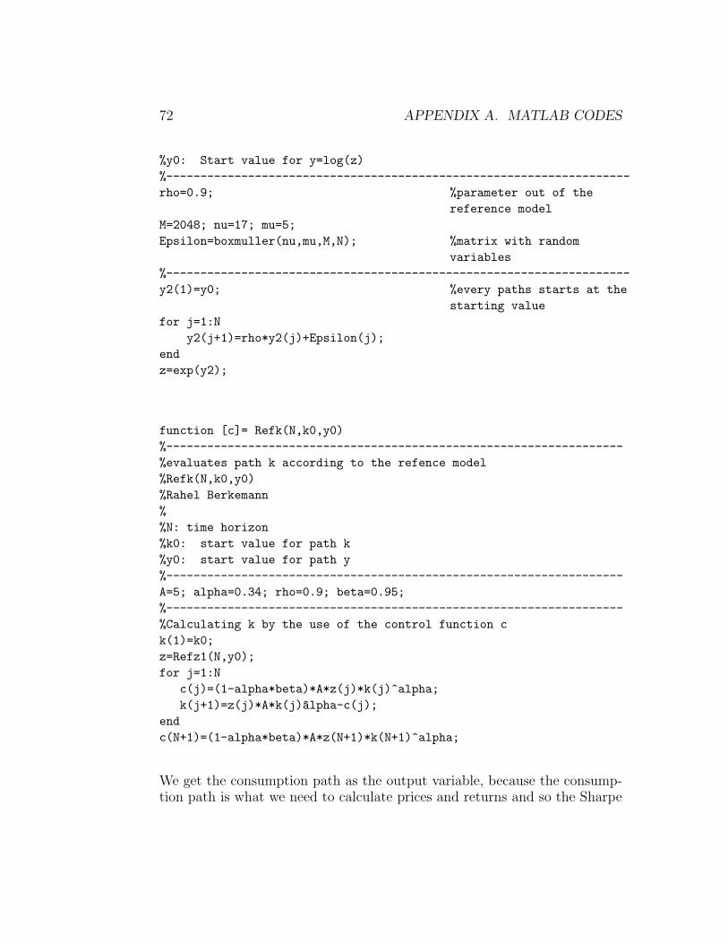
72 APPENDIX A. MATLAB CODES
%y0: Start value for y=log(z)%--------------------------------------------------------------------rho=0.9; %parameter out of the
reference modelM=2048; nu=17; mu=5;Epsilon=boxmuller(nu,mu,M,N); %matrix with random
variables%--------------------------------------------------------------------y2(1)=y0; %every paths starts at the
starting valuefor j=1:N
y2(j+1)=rho*y2(j)+Epsilon(j);endz=exp(y2);
function [c]= Refk(N,k0,y0)%-------------------------------------------------------------------%evaluates path k according to the refence model%Refk(N,k0,y0)%Rahel Berkemann%%N: time horizon%k0: start value for path k%y0: start value for path y%-------------------------------------------------------------------A=5; alpha=0.34; rho=0.9; beta=0.95;%-------------------------------------------------------------------%Calculating k by the use of the control function ck(1)=k0;z=Refz1(N,y0);for j=1:N
c(j)=(1-alpha*beta)*A*z(j)*k(j)^alpha;k(j+1)=z(j)*A*k(j)alpha-c(j);
endc(N+1)=(1-alpha*beta)*A*z(N+1)*k(N+1)^alpha;
We get the consumption path as the output variable, because the consump-tion path is what we need to calculate prices and returns and so the Sharpe

A.2. MATLAB CODES FOR THE TIME SERIES SOLUTION 73
Ratio. The main MATLAB code we need for our analysis is the following,where we calculate the Upper Bound and the Sharpe Ratio.
function SR(N,k0,y0)%--------------------------------------------------------------------%Computation of the upper bound SB and the Sharpe Ratio for the%Time Series approach%SR(N,k0,y0)%Rahel Berkemann% %N: Time horizon%k0: start value for k%y0: Start value for y=log(z)%--------------------------------------------------------------------A=5; alpha=0.34; rho=0.9; beta=0.95;%--------------------------------------------------------------------%Computation of cc=Refk(N,k0,y0);%--------------------------------------------------------------------%Computation of m(x)with x=(k,z)for i=1:N-1
m t(i)=beta*c(i)/c(i+1);end%--------------------------------------------------------------------% Computation of E(m(x))Exp m=1/(N-1)*sum(m t);%--------------------------------------------------------------------%Computation of the risk-free interest rate R f(x)R f=1./Exp m;%--------------------------------------------------------------------%Computation of the Variance of m(x)Var m t=(m t-Exp m*ones(1,N-1)).2;Var m=1/(N-1)*sum(Var m t)%--------------------------------------------------------------------%Computation of the Standard deviation of m(x)SD m=sqrt(Var m);%--------------------------------------------------------------------%Computation of the Upper Bound SBSB=SD m/Exp m;%--------------------------------------------------------------------%Computing Sharpe Ratios

74 APPENDIX A. MATLAB CODES
%Computation of p(x) with d(x)=c(x)p=beta/(1-beta)*c;%--------------------------------------------------------------------%Computation of R(x)for i=1:N-1
R t(i)=(c(i+1)+p(i+1))./p(i);end%--------------------------------------------------------------------%Computing E(R(x))Exp R=1/(N-1)*sum(R t);%--------------------------------------------------------------------%Comptation of the Covariance of R(x) and m(x);Cov R m t=(R t-Exp R*ones(1,N-1)).*m t-Exp m*ones(1,N-1));Cov R m=1/(N-1)*sum(Cov R m t);%Computation of Var(R(x)) and SD(R(x))Var R t=(R t-Exp R*ones(1,N-1).^2;Var R=1/(N-1)*sum (Var R t);SD R=sqrt(Var R);%---------------------------------------------------------------------%Computation of the Sharpe Ratio via the Covariance formulaSR Cov=(-R f*Cov R m)/SD R%---------------------------------------------------------------------%Computation of the Sharpe Ratio via the standard formulaSR stand=(Exp R-R f)/SD R
A.3 MATLAB codes for the Random Vari-
able solution
The second approach for solving the reference model was to look at thevariable m(x) as being a random variable itself. The MATLAB codes to thatapproach are given in this section. I start with the main code for the SharpeRatio analysis. All additional functions, i.e. the codes for the computation ofthe expectations, variances and covariances, are listed afterwards. Since weneed this programme in chapter 7 as well when we look for different outcomesdepending on σε we include a variable s for the standard deviation and a forthe interval boundarys.
A.3. MATLAB CODES FOR THE RANDOM VARIABLE SOLUTION 75
I start with the programme for figuring out the interval boundarys, whichjust worked by looking at the plot computed by the following programme.
function density(s,a)%-------------------------------------------------------------------%plots the density function for epsilon%density(s,a)%s: standard deviation for epsilon%a: interval boundary%-------------------------------------------------------------------m=a/20;epsilon=(-a:m:a);density=1/(sqrt(2*pi)*s).*exp(-1/2*(epsilon.^2./(s^2)));plot(epsilon,density,’r’)ylabel(’f(epsilon)’)xlabel(’epsilon’)
Now, the main programme for calculating the Sharpe Ratios in the randomvariable model is given. ”quad” is a MATLAB internal routine that calculatesthe integral by using Simpson’s Quadrature. The command scale=quad(@Exp m,-a,a,1.e-9,[],y0,k0,s); loads the programme Exp m, it calculates the integral inthe intrval [−a, a], 1.e-9 is the accuracy that quad should use for computa-tion, y0, k0 are the initial values and s is the parameter for the standardvariable.
function RV(y0,k0,s,a)%---------------------------------------------------------------------%Computing random variable m%RV(y0,k0)%Rahel Berkemann%%y0: start value for y%k0: start value for k%---------------------------------------------------------------------beta=0.95; alpha=0.34; rho=0.9; A=5;%---------------------------------------------------------------------scale=quad(@Exp m,-a,a,1.e-9,[],y0,k0,s);Exp m=quad(@Exp m,-a,a,1.e-9,[],y0,k0,s,scale)Var m=quad(@Var m,-0.032,0.032,1.e-9,[],y0,k0,s,scale,Exp m);
76 APPENDIX A. MATLAB CODES
SD m=sqrt(Var m);R f=1/Exp mExp R=quad(@Exp R,-a,a,1.e-9,[],y0,k0,s,scale)Var R=quad(@Var R,-a,a,1.e-9,[],y0,k0,s,scale,Exp R);SD R=sqrt(Var R);%---------------------------------------------------------------------%Computing the Upper BoundSB=SD m/Exp m%---------------------------------------------------------------------%Computing the Sharpe Ratio%1. SR CovCov R m=quad(@Cov R m,-a,a,1.e-9,[],y0,k0,s,scale,Exp m,Exp R);SR Cov=(-R f*Cov R m)/SD R%2. SR standSR stand=abs((Exp R-R f/SD R)
The following programmes that are listed are the ones evoked by the mainprogramm.
function [m]= Exp m(x,y0,k0,s,scale)%---------------------------------------------------------------------beta=0.95; alpha=0.34; rho=0.9; A=5;%---------------------------------------------------------------------c0=(1-alpha*beta)*A*exp(y0)*k0^alpha;y1=rho*y0+x;k1=exp(y0)*A*k0^alpha-c0;c1=(1-alpha*beta)*A*exp(y1)*k1^alpha;m=beta*c0./c1.*(1/sqrt(2*pi)*s).*(1/scale)
.*exp(-(x.^2./(2*s^2))));
function [m]= Var m(x,y0,k0,s,scale,Exp m)%---------------------------------------------------------------------beta=0.95; alpha=0.34; rho=0.9; A=5;%---------------------------------------------------------------------c0=(1-alpha*beta)*A*exp(y0)*k0^alpha;y1=rho*y0+x;k1=exp(y0)*A*k0^alpha-c0;c1=(1-alpha*beta)*A*exp(y1)*k1^alpha;
A.3. MATLAB CODES FOR THE RANDOM VARIABLE SOLUTION 77
m=(beta*c0./c1-Exp m).^2.*(1/scale).*(1/sqrt(2*pi)*s).*exp(-(x.^2./(2*s^2))));
function [R]= Exp R(x,y0,k0)%---------------------------------------------------------------------beta=0.95; alpha=0.34; rho=0.9; A=5;%---------------------------------------------------------------------c0=(1-alpha*beta)*A*exp(y0)*k0^alpha;y1=rho*y0+x;k1=exp(y0)*A*k0^alpha-c0;c1=(1-alpha*beta)*A*exp(y1)*k1^alpha;p0=beta/(1-beta)*c0;p1=beta/(1-beta)*c1;R=(c1+p1)./p0.*(1/sqrt(2*pi)*0.008).*
(1/scale).*exp(-(x.^2./(2*0.008^2))));
function [R]= Var R(x,y0,k0,Exp R)%---------------------------------------------------------------------beta=0.95; alpha=0.34; rho=0.9; A=5;%---------------------------------------------------------------------c0=(1-alpha*beta)*A*exp(y0)*k0^alpha;y1=rho*y0+x;k1=exp(y0)*A*k0^alpha-c0;c1=(1-alpha*beta)*A*exp(y1)*k1^alpha;p0=beta/(1-beta)*c0;p1=beta/(1-beta)*c1;R=((c1+p1)./p0-Exp R).^2.*(1/scale)
.*(1/sqrt(2*pi)*0.008).*exp(-(x.^2./(2*0.008^2))));
function [R]= Cov R m(x,y0,k0,Exp m,Exp R)%---------------------------------------------------------------------beta=0.95; alpha=0.34; rho=0.9; A=5;%---------------------------------------------------------------------c0=(1-alpha*beta)*A*exp(y0)*k0^alpha;y1=rho*y0+x;k1=exp(y0)*A*k0^alpha-c0;c1=(1-alpha*beta)*A*exp(y1)*k1^alpha;
78 APPENDIX A. MATLAB CODES
p0=beta/(1-beta)*c0;p1=beta/(1-beta)*c1;R=(((c1+p1)./p0-Exp R).*(beta*c0./c1-Exp m)).*(1/scale)
.*(1/sqrt(2*pi)*0.008).*exp(-(x.^2./(2*0.008^2))));
A.4 MATLAB codes for the Check
The programme to check for correctness as discussed in chapter 7.1 lookssimilar to the programme used in chapter 5. The only things we change werealready discussed in chapter 7.1.
function SR control(N,y0,k0)%--------------------------------------------------------------------%checks for correctness of the code SR(N,y0,k0)%Time Series approach%SR(N,k0,y0)%Rahel Berkemann% %N: Time horizon%k0: start value for k%y0: Start value for y=log(z)%--------------------------------------------------------------------
%Lagged FibonacciM=2048; nu=17; mu=5;rand(’seed’,2);X1=M*rand(1,max(mu,nu));X2=M*rand(1,max(mu,nu));for i=max(mu,nu)+1:N+max(mu,nu)
X1(i)=mod(X1(i-mu)-X1(i-nu),M);U1(i-max(mu,nu))=X1(i)/M;X2(i)=mod(X2(i-mu)-X2(i-nu),M);U2(i-max(mu,nu))=X2(i)/M;
end%--------------------------------------------------------------------
%boxmuller Z=sqrt(-2*log(U1)).*cos(2*pi*U2);E Z=1/N*sum(Z);
A.4. MATLAB CODES FOR THE CHECK 79
Var Z=1/N*sum((Z-E Z*ones(1,N)).^2);SD Z=sqrt(Var Z);%--------------------------------------------------------------------
%RV with mean 0 and SD 0.008Eps=0.008*Z;E Eps=1/N*sum(Eps);Var Eps=1/N*sum((Eps-E Eps*ones(1,N)).^2);SD Eps=sqrt(Var Eps);%--------------------------------------------------------------------
%Initialising parameters for the stochastic growth modelbeta=0.95; alpha=0.34; rho=0.9; A=5;%--------------------------------------------------------------------
%Calculating path zy(1)=y0;for t=1:N
y(t+1)=rho*y0+Eps(t);endz=exp(y);%--------------------------------------------------------------------
%Computing k and ck(1)=k0;c(1)=(1-alpha*beta)*z(1)*A*k(1)^alpha;k(2)=exp(y0)*A*k0^alpha-c(1);for t=2:N
c(t)=(1-alpha*beta)*z(t)*A*k(2)^alpha;end%--------------------------------------------------------------------
%Computing mfor t=1:N
m t(t)=beta*(c(1)/c(t+1));endExp m=1/N*sum(m t)Var m=1/N*sum((m t-Exp m*ones(1,N)).^2);SD m=sqrt(Var m)%--------------------------------------------------------------------

80 APPENDIX A. MATLAB CODES
%Computing the Upper Bound S BS B=SD m/Exp m%--------------------------------------------------------------------
%Risk-free interest rateR f=1/Exp m%--------------------------------------------------------------------
%Computing p(x) with d(x)=c(x)p=beta/(1-beta)*c;%--------------------------------------------------------------------
%Computing R(x)for i=1:N
R t(i)=(c(i+1)+p(i+1))/p(1);end%--------------------------------------------------------------------
%Computing E(R(x))Exp R=1/N*sum(R t);%--------------------------------------------------------------------
%Computing CovariancesCov R m t=(R t-Exp R*ones(1,N)).*(m t-Exp m*ones(1,N));Cov R m=1/N*sum(Cov R m t);%--------------------------------------------------------------------
%Computing Var(R(x)) and SD(R(x))Var R t=(R t-Exp R*ones(1,N)).^2;Var R=1/N*sum(Var R t);SD R=sqrt(Var R);%--------------------------------------------------------------------
%Computing Sharpe Ratio via CovarianceSR cov=(-R f*Cov R m)/SD R%--------------------------------------------------------------------
%Computing Sharpe Ratio with standard formulaSR stand=abs((Exp R-R f)/SD R)

A.5. MATLAB CODES FOR CORRELATIONS 81
A.5 MATLAB codes for Correlations
We have one main programm giving us the Correlations and Covariances forour analysis in chapter 7. The first part of the following programm givesus the Correlations and Covariances for the time series case, whereas thesecond part gives us the ones for the random variable approach. For thelatter additional programmes are used for computing the integrals neededfor the calculation of covariances in the random variable case. The inputparamter s for the standard deviation needed in the random variable part isset to 0.008. When we calculate correlations for another standard deviationthe boxmuller.m programme used in the time series part needs to be adjusted,i.e. 0.008*Z has to be changed to s*Z.
function cor(N,y0,k0,s,a)%--------------------------------------------------------------------%Calculates correlations between time series %cor(N,k0,y0,s,a)%Rahel Berkemann% %N: Time horizon%k0: start value for k%y0: Start value for y=log(z)%--------------------------------------------------------------------
%Initialising parameters for the stochastic growth modelbeta=0.95; alpha=0.34; rho=0.9; A=5;%--------------------------------------------------------------------
%Expectation and Variance of EpsilonM=2048; nu=17; mu=5;Eps=boxmuller(nu,mu,M,N);E Eps=1/N*sum(Eps);V Eps=1/N*sum((Eps-E Eps).^2);%--------------------------------------------------------------------
%Covariance of z and cz=Refz(N,y0);E z=1/(N+1)*sum(z);Var z t=(z-E z*ones(1,N+1)).^2;Var z=1/(N+1)*sum((z-E z*ones(1,N+1)).^2);
c=Refk(N,k0,y0);
82 APPENDIX A. MATLAB CODES
E c=1/(N+1)*sum(c);Var c=1/(N+1)*sum((c-E c*ones(1,N+1)).^2);
Cov z c t=(z-E z*ones(1,N+1)).*(c-E c*ones(1,N+1));Cov z c=1/(N+1)*sum(Cov z c t);
Cor z c=Cov z c/(sqrt(Var z)*sqrt(Var c))
%--------------------------------------------------------------------
%Covariance of k and zk2(1)=k0;fort=1:N
k2(t+1)=A*z(t)*k2(t)^alpha-c(t);endE k=1/(N+1)*sum(k2);Var k=1/(N+1)*sum((k2-E k*ones(1,N+1)).^2);
Cov z k t=(z-E z*ones(1,N+1)).*(k2-E k*ones(1,N+1));Cov z k=1/(N+1)*sum(Cov z k t);
Cor z k=Cov z k/(sqrt(Var z)*sqrt(Var k))%--------------------------------------------------------------------
%Covariance of p and z%Berechung von p(x) mit d(x)=c(x)p=beta/(1-beta)*c;E p=1/(N+1)*sum(p);Var p=1/(N+1)*sum((p-E p*ones(1,N+1)).^2);Cov z p t=(z-E z*ones(1,N+1)).*(p-E p*ones(1,N+1));Cov z p=1/(N+1)*sum(Cov z p t);
Cor z p=Cov z p/(sqrt(Var z)*sqrt(Var p))%--------------------------------------------------------------------
%Covariance of k^alpha and ck alpha=k2.^alpha;E k alpha=1/(N+1)*sum(k alpha);Var k alpha=1/(N+1)*sum((k alpha-E k alpha*ones(1,N+1)).^2);
Cov k alpha c t=(c-E c*ones(1,N+1)).*(k alpha-E k alpha*ones(1,N+1));
A.5. MATLAB CODES FOR CORRELATIONS 83
Cov k alpha c=1/(N+1)*sum(Cov k alpha c t);
Cor k alpha c=Cov k alpha c/(sqrt(Var c)*sqrt(Var k alpha))%--------------------------------------------------------------------%--------------------------------------------------------------------
%Covariance in the random variable casescale = quad(@scale,-a,a,1.e-15,[],s);
%Exp Eps= quad(@Exp Eps,-0.032,0.032,1.e-9,[],y0,k0)%Covariance of z and cExp z= quad(@Exp z,-a,a,1.e-9,[],y0,k0,s,scale);Var z= quad(@Var z,-a,a,1.e-9,[],y0,k0,s,scale,Exp z);Exp c= quad(@Exp c,-a,a,1.e-9,[],y0,k0,s,scale);Var c= quad(@Var c,-a,a,1.e-9,[],y0,k0,s,scale,Exp c);Cov z c = quad(@Cov z c,-a,a,1.e-9,[],y0,k0,s,scale,Exp z,Exp c);
Cor2 z c=Cov z c/(sqrt(Var z)*sqrt(Var c))%-------------------------------------------------------------------
%Covariance of k and zc0=(1-alpha*beta)*A*exp(y0)*k0^alpha;k1=exp(y0)*A*k0^alpha-c0;Exp k=k1;Var k=(k1-Exp k);Cov z k = quad(@Cov z k,-a,a,1.e-9,[],y0,k0,s,scale,Exp z,Exp k)%-------------------------------------------------------------------
%Covariance of p and zExp p=beta/(1-beta)*Exp c;Var p = (beta/(1-beta))^2*Var c;Cov z p= quad(@Cov z p,-a,a,1.e-9,[],y0,k0,s,scale,Exp z,Exp p);
Cor2 z p=Cov z p/(sqrt(Var z)*sqrt(Var p))%--------------------------------------------------------------------
%Covariance of k^alpha and cc0=(1-alpha*beta)*A*exp(y0)*k0^alpha;k1=exp(y0)*A*k0^alpha-c0;Exp k alpha=k1^alpha;Var k alpha=k1^alpha-Exp k alpha;

84 APPENDIX A. MATLAB CODES
Cov k alpha c =quad(@Cov k alpha c,-a,a,1.e-9,[],y0,k0,s,scale,Exp c,Exp k alpha)
%--------------------------------------------------------------------
Next, the additional programmes needed in the random variable case, arelisted. These programmes are loaded by the same commands that were ex-plained in appendix A.3.
function [y]= Exp z(x,y0,k0,s,scale)%-------------------------------------------------------------------%Initialisierungenbeta=0.95; alpha=0.34; rho=0.9; A=5;%-------------------------------------------------------------------c0=(1-alpha*beta)*A*exp(y0)*k0^alpha;y1=rho*y0+x;k1=exp(y0)*A*k0^alpha-c0;c1=(1-alpha*beta)*A*exp(y1)*k1^alpha;y=exp(y1).*(1/scale).*(1/(sqrt(2*pi)*s).*exp(-(x.^2./(2*s^2))));
function [y]= Var y(x,y0,k0,s,scale,Exp z)%-------------------------------------------------------------------%Initialisierungenbeta=0.95; alpha=0.34; rho=0.9; A=5;%-------------------------------------------------------------------c0=(1-alpha*beta)*A*exp(y0)*k0^alpha;y1=rho*y0+x;k1=exp(y0)*A*k0^alpha-c0;c1=(1-alpha*beta)*A*exp(y1)*k1^alpha;y=(exp(y1)-Exp z).^2
.*(1/scale).*(1/(sqrt(2*pi)*s).*exp(-(x.^2./(2*s^2))));
function [c]= Exp c(x,y0,k0,s,scale)%-------------------------------------------------------------------%Initialisierungenbeta=0.95; alpha=0.34; rho=0.9; A=5;%-------------------------------------------------------------------

A.5. MATLAB CODES FOR CORRELATIONS 85
c0=(1-alpha*beta)*A*exp(y0)*k0^alpha;y1=rho*y0+x;k1=exp(y0)*A*k0^alpha-c0;c1=(1-alpha*beta)*A*exp(y1)*k1^alpha;c=c1.*(1/scale).*(1/(sqrt(2*pi)*s).*exp(-(x.^2./(2*s^2))));
function [c]= Var c(x,y0,k0,s,scale,Exp c)%-------------------------------------------------------------------%Initialisierungenbeta=0.95; alpha=0.34; rho=0.9; A=5;%-------------------------------------------------------------------c0=(1-alpha*beta)*A*exp(y0)*k0^alpha;y1=rho*y0+x;k1=exp(y0)*A*k0^alpha-c0;c1=(1-alpha*beta)*A*exp(y1)*k1^alpha;c=(c1-Exp c).^2
.*(1/scale).*(1/(sqrt(2*pi)*s).*exp(-(x.^2./(2*s^2))));
function [y]= Cov z c(x,y0,k0,s,scale,Exp z,Exp c)%-------------------------------------------------------------------%Initialisierungenbeta=0.95; alpha=0.34; rho=0.9; A=5;%-------------------------------------------------------------------c0=(1-alpha*beta)*A*exp(y0)*k0^alpha;y1=rho*y0+x;k1=exp(y0)*A*k0^alpha-c0;c1=(1-alpha*beta)*A*exp(y1)*k1^alpha;y=(exp(y1)-Exp z).*(c1-Exp c)
.*(1/scale).*(1/(sqrt(2*pi)*s).*exp(-(x.^2./(2*s^2))));
function [y]= Cov z k(x,y0,k0,s,scale,Exp z,Exp k)%-------------------------------------------------------------------%Initialisierungenbeta=0.95; alpha=0.34; rho=0.9; A=5;%-------------------------------------------------------------------c0=(1-alpha*beta)*A*exp(y0)*k0^alpha;y1=rho*y0+x;

86 APPENDIX A. MATLAB CODES
k1=exp(y0)*A*k0^alpha-c0;c1=(1-alpha*beta)*A*exp(y1)*k1^alpha;y=(exp(y1)-Exp z).*(k1-Exp k)
.*(1/scale).*(1/(sqrt(2*pi)*s).*exp(-(x.^2./(2*s^2))));
function [y]= Cov z p(x,y0,k0,s,scale,Exp z,Exp p)%-------------------------------------------------------------------%Initialisierungenbeta=0.95; alpha=0.34; rho=0.9; A=5;%-------------------------------------------------------------------c0=(1-alpha*beta)*A*exp(y0)*k0^alpha;y1=rho*y0+x;k1=exp(y0)*A*k0^alpha-c0;c1=(1-alpha*beta)*A*exp(y1)*k1^alpha;y=(exp(y1)-Exp z).*(beta/(1-beta)*c1-Exp p)
.*(1/scale).*(1/(sqrt(2*pi)*s).*exp(-(x.^2./(2*s^2))));
function [y]= Cov k alpha c(x,y0,k0,s,scale,Exp c,Exp k alpha)%-------------------------------------------------------------------%Initialisierungenbeta=0.95; alpha=0.34; rho=0.9; A=5;%-------------------------------------------------------------------c0=(1-alpha*beta)*A*exp(y0)*k0^alpha;y1=rho*y0+x;k1=exp(y0)*A*k0^alpha-c0;c1=(1-alpha*beta)*A*exp(y1)*k1^alpha;y=(c1-Exp c).*(k1.^alpha-Exp k alpha)
.*(1/scale).*(1/(sqrt(2*pi)*s).*exp(-(x.^2./(2*s^2))));
A.6 MATLAB code for the Loss Aversion model
The following MATLAB codes calculate the return of risky assets and therisk-free return by loading a file where the given return datas are stored.This is done by the command ’load’. Since the only thing that is varied isthe factor b0, just one ”example” programme is given in this chapter. The

A.6. MATLAB CODE FOR THE LOSS AVERSION MODEL 87
paramter j, j ∈ 0, 001, 005, 01, 05, 3, 10, therefore denotes the factor usedfor b0, where for example 001 means 0.01. In order to load the files as stated inthe programme, they have to be stored in the same folder as the programme.All programmes and files are on the included CD.
function bjT = load(’bj Reihe.asc’);R t=T(:,8);R f t=T(:,9);N=length(R t);%----------------------------------------------------------%Computing E(R(x));Exp R=1/N*sum(R t)Var R t=(R t-Exp R*ones(N,1)).^2;Var R=1/N*sum(Var R t);SD R=sqrt(Var R)%----------------------------------------------------------%Computing R fR f=1/N*sum(R f t)%-------------------------------------------------------%Computing Sharpe Ratio with standard formulaSR stand=abs((Exp R-R f)/SD R)

Appendix B
The included CD
The CD included stores all relevant programmes and files used in this thesis.The set-up as follows: main folder is called Methods for Calculating SharpeRatios and contains the following folders and programms:
1. Folder Path k
(a) RWfibonacci path.m
(b) boxmuller path.m
(c) Refz path.m
(d) Refk picture.m
2. Folder Time Series approach
(a) RWfibonacci.m
(b) boxmuller.m
(c) Refz.m
(d) Refk.m
(e) SR.m
3. Folder Random Variable approach
(a) RV.m
88

89
(b) density.m
(c) scale.m
(d) Exp m.m
(e) Var m.m
(f) Exp R.m
(g) Var R.m
(h) Cov R m.m
4. Folder Check
(a) SR control.m
5. Folder Correlations
(a) cor.m
(b) RWfibonacci.m
(c) boxmuller.m
(d) Refz.m
(e) Refk.m
(f) scale.m
(g) Exp z.m
(h) Var z.m
(i) Exp c.m
(j) Var c.m
(k) Cov z c.m
(l) Cov z p.m
(m) Cov z k.m
(n) Cov k alpha c.m
6. Folder Loss Aversion model
(a) data files b0 reihe, b001 reihe, b005 reihe, b01 reihe, b05 reihe,b3 reihe and b10 reihe.
(b) programmes b0.m, b001.m, b005.m, b01.m, b05.m, b3.m and b10.m.

Bibliography
[1] John Black, Dictionary of Economics, Oxford University Press, Ox-ford, New York, 2002.
[2] W. Brock, L. Mirman, Optimal economic growth and uncertainty:the discounted case, Journal of Economic Theory 4: 479-513, 1972.
[3] Y. S. Chow and H. Teicher, Probability Theory - Independenceinterchangeability Martingales,Springer Verlag, New York, 1978.
[4] J. Cochrane, Asset Pricing, Princeton University Press, Princeton,2001.
[5] P. M. Geraats, Intertemporal Optimization under Uncertainty, Lec-ture Notes, Cambridge, 2002.
[6] W. H. Greene, Econometric Analysis, Prentice Hall, Inc., New Jersey,2000.
[7] L. Grune and W. Semmler, Solving Asset Pricing Models withStochastic Dynamic Programming, 2002.
[8] L. Grune and W. Semmler, Asset Pricing with Loss Aversion, Work-ing Paper No. 92, University of Bielefeld, Department of Economics,Center for Empirical Macroeconomics.
[9] L. Grune, Error estimation and adaptive discretization for the discretestochastic Hamilton-Jacobi-Bellman equation, Springer-Verlag, 2004.
[10] M. Gunther and A. Jungel, Finanzderivate mit MATLAB, Vieweg,Wiesbaden, 2003.
90

BIBLIOGRAPHY 91
[11] A. W. Lo, The Statistics of Sharpe Ratios,AIMR, 2002.
[12] D. Romer, Advanced Macroeconomics, McGraw-Hill, New York, 2001.
[13] T. Soderstrom, Discrete-time Sochastic Systems, Springer, London,2002.
[14] W. W. S. Wei, Time Series Analysis, Addison-Wesley Publishing Com-pany, 1994.

92 BIBLIOGRAPHY

Erklarung
Hiermit erklare ich, dass die vorliegende Arbeit selbststandig und unter Ver-wendung der angegebenen Quellen und Hilfsmittel angefertigt habe.
Diese Arbeit hat in gleicher oder ahnlicher Form noch keiner anderen Prufungsbehordevorgelegen.
Bayreuth, den 13. Juni 2006 ..........................
Rahel Berkemann
93


