Methods for Cole Parameter

Estimation from Bioimpedance Spectroscopy Measurements

A Comparative Study

David Ayllón

MASTER DEGREE THESIS 15 ECTS, 2008-09 SWEDEN BIOMEDICAL ENGINEERING

THESIS Nº 5/2008

ii

Methods for Cole Parameter Estimation from Bioimpedance Spectroscopy Measurements. A Comparative Study.

David Ayllón

Master Degree Thesis Subject Category: Medical Technology, Signal Processing

University of Borås

School of Engineering

SE- 501 90 BORAS

Telephone +46 33 435 4640

Examiner: Fernando Seoane Martínez

Supervisor: Fernando Seoane Martínez

Date: 2009 Jun 8th

Keywords: Electrical Bioimpedance Spectroscopy, Cole Model, Statistical Analysis.

iii

ABSTRACT

There are several applications of Electrical Bioimpedance Spectroscopy (EBIS) and Multi-Frequency (MF-EBI) that use the Cole parameters as indicators and base of the data analysis. Therefore to fit complex EBI measurements data onto the Cole equation is a very common practice within MF-EBI and EBIS. The work done in this thesis has compared different methods and approaches to fit EBI measurements into the Cole equation and consequently to estimate the Cole parameters. Three of the methods included in the study are based on the use of Non-Linear Least Squares method over the spectrum of the EBI, one using the real part only, a second using the imaginary part and the third using the combination of both. Furthermore, an alternative fitting approach done on the impedance plane, without using frequency information has been implemented and include in the comparison.

For the study of the performance of these methods, noisy impedance data have been

generated according to a realistic noise model. Moreover, the impact that variations of noise level have on the different fittings methods has been assessed and its results have been discussed.

Results show that the four methods perform relatively well but the best fitting in terms of

Standard Error of Estimate is the obtained from the resistance part only, independently of the noise level. The results support the possibility of measuring only the resistance of the complex EBI to accurate fit the Cole equation or estimate the Cole parameters.

iv

ACKNOWLEDGEMENTS

I would like to appreciate all the effort and dedication that my thesis director, Dr. Fernando Seoane, has provided me with during the realization of this final degree work. His daily support has been fundamental to solve all the problems found along the way.

I am also grateful for the help that Dr. Roberto Gil has offered to me. He always gave a

hand when I needed it. I would like to thank my colleagues, Tony, Rubén, Javi, Ruth G., Juan Carlos and Ruth

P., because they have done more enjoyable to work every day in this work and we have spent very good moments together.

And about all I have to thanks to my family and friends, especially Gema, who

encouraged me to take the decision to leave everything behind and engage my-self in the adventure of studying this master programme in Sweden with the aim of shifting my career towards research.

v

TABLE OF CONTENTS

Abstract .............................................................................................................................. iiiAcknowledgements ............................................................................................................ ivTable of Contents .................................................................................................................vList of Acronyms ............................................................................................................... viiCHAPTER 1 Thesis Introduction .................................................................................. 81.1. Introduction ................................................................................................................. 81.2. Motivation .................................................................................................................... 81.3. Goal .............................................................................................................................. 81.4. Work Done ................................................................................................................... 81.5. Structure of the Thesis Report .................................................................................... 81.6. Out of Scope ................................................................................................................. 9CHAPTER 2 Background ............................................................................................ 102.1. Curve Fitting.............................................................................................................. 10

2.1.1. Complex Curve Fitting ............................................................................................. 102.1.2. Non-Linear Curve Fitting ......................................................................................... 102.1.3 Non-Linear Least Squares Method ............................................................................... 10

2.2. EBI Measurements .................................................................................................... 112.3. Cole Equation ............................................................................................................ 12CHAPTER 3 methods .................................................................................................. 133.1. Curve Fitting and Cole Parameters Estimation with the NLLS Method ................ 133.2. Initial Values Estimation for NLLS ......................................................................... 133.3. Cole Parameters Estimation on the Impedance Plane ............................................ 143.4. Cole Fitting and Error Analysis ............................................................................... 183.5. EBI data generation .................................................................................................. 183.6. Noise Model ............................................................................................................... 19CHAPTER 4 Results ..................................................................................................... 204.1. Fitting Results............................................................................................................ 204.2. Frequency Based Estimation Results ....................................................................... 224.3. Impedance Plane Estimation Results ....................................................................... 224.4. Cole Parameters Estimation Results ........................................................................ 22

vi

4.5. Noise-Error Results ................................................................................................... 224.6. Noise Influence in R, X, |Z| and Cole Plot Curve Fitting ........................................ 254.7. Noise Influence in Cole Parameters Estimation ...................................................... 25CHAPTER 5 Discussion ............................................................................................... 265.1 Methods Performance ................................................................................................ 265.2 Noise Influence ........................................................................................................... 265.3 Other Possible Influencing Factors on the Methods Performance ......................... 26CHAPTER 6 Conclusions & Future Work ................................................................. 286.1 General Conclusions .................................................................................................. 286.2. Future work ............................................................................................................... 28REFERENCES ................................................................................................................ 29Appendix A papercontribution to IEEE-EMBC2009 ..................................................... 30

vii

LIST OF ACRONYMS

EBI Electrical Bioimpedance SEE Standard Error of Estimate SNR Signal to Noise Rate MF-EBI Multi-Frequency Electrical Bioimpedance EBIS Electrical Bioimpedance Spectroscopy NLLS Non-Linear Least Squares Z Impedance R Resistance X Reactance

8

CHAPTER 1

THESIS INTRODUCTION

1.1. Introduction Nowadays, measuring the Electrical Bioimpedance (EBI) in humans and animals is a

common practice and has different clinical applications like skin cancer detection known as electronic biopsy(Aberg, Nicander et al. 2004), respiration monitoring using impedance Pneumography, determine Cardiac Stroke Volume and Cardiac Output by means of impedance Cardiography and assessment on body composition estimation (Matthie, Withers et al. 1992)

Several applications based on MF-EBI and EBIS have the common step of fitting the EBI

measured data to a model described by the Cole equation by estimating the Cole parameters (Gudivaka, Schoeller et al. 1999).

1.2. Motivation

Cole parameter estimation is a very important task in several EBI applications that creates a very important dependency of the characteristic of the measured data and therefore in the electronic instrumentation used to acquire data. To find Cole parameter estimation approaches that decrease the remands on the measured EBI would influence in the whole design of the impedance spectrometers and may enable the implementation of simpler and more affordable electrical devices.

1.3. Goal The main goal of this thesis is to test and compare the performance of different

approaches and methods to fit EBI data to the Cole Equation and estimate the Cole Parameters. A secondary purpose is to find a realistic noise model for EBI measurements.

1.4. Work Done In this thesis, four different fitting methods according with two different approaches have

been introduced and compared in terms of Standard Error of Estimate (SEE). Experimental measurement noise has been studied and generated and finally, EBI data with different levels of added noise have been fitted to the Cole Equation with the four different methods estimating the Cole parameters from the measurements as well.

1.5. Structure of the Thesis Report The whole thesis report is organized in 6 chapters and final section for the references and

one appendix including the conference paper produced with the results of this thesis.

9

Chapter 1 contains the introduction part of this thesis report. Chapter 2 provides a brief

background about curve fitting methods, EBI measurements and Cole equation. Chapter 3 describes the theory of the methods used in this thesis while Chapter 4 shows the obtained results. Finally Chapter 5 discuss the results and the work done and Chapter 6 ends the report with the conclusion and propose future work to be done in this line of Cole fitting and pre-processing of EBI data for multifrequency or spectroscopy analysis.

.

1.6. Out of Scope Some issues has been left out of scope of this thesis and exposed in the last section as

future work. These points are basically the study of the impact of using different frequency distributions to perform the EBI measurements and the curve fitting. Any attempt to compensate for measurement errors like measurement noise or parasitic effects prior to the Cole fitting or Cole parameter estimation.

10

CHAPTER 2

BACKGROUND

2.1. Curve Fitting Curve Fitting is a technique that provides a curve and its mathematical function that best

approximate a given set of points. Sometimes additional constraints can be introduced into the problem. There are two approaches to solve the problem, interpolation and regression analysis, being the latter the one we focus on (Coope 1993).

Regression analysis is a technique that tries to model numerical data points of a

dependant variable and one of more independent variables. The model relates the dependent variable as function of the independent variables, also know as parameters. This model can be linear or non-linear. The most common method for regression is Least Squares method (Wild 1989).

2.1.1. Complex Curve Fitting When the set of data points to fit is complex, to find the best curve that approximates the

points is not a trivial task. Generally, all methods that perform complex curve fitting split data into real and imaginary parts, concatenating both as input data and evaluating the complex function. Once the curve fitting is done then the complex data is reassembled.

2.1.2. Non-Linear Curve Fitting Non-Linear curve fitting consists in a case of regression where the data points to fit are

modelled by a function that is a non-linear combination of one of more parameters or one of more independent variables.(Box, Davies et al. 1969)

Normally, data is fitted following an algorithm based on successive approximations, like

it is the case in Non-Linear Least Squares method for instance.

2.1.3 Non-Linear Least Squares Method When using this method the algorithm estimates the best coefficients of a defined non-

linear model that fits the measured point to the curve described by the model. The method tries to minimize the summed squared of the error between the data series and the fitted model as indicated in (2.1):

2

1 1

2 )(minmin = =

−=N

i

N

iiii yye

(2.1) where ei is the error of the i-th data point, and N is the total number of data points

included in the fit.

11

The method can be implemented in Matlab with the function fit that provides an

estimation of one curve that fits a given measurement as input data, to a non-linear real parametric model with coefficients.

The method works as an iterative process following the next steps:

1- An initial estimation of the coefficients should be provided 2- Calculate the fitted curve according the new coefficients. 3- Adjust the coefficients and check if the fit improves in terms of summed squared

of error. This is done with ‘Trust-region’ algorithm. 4- Repeat process from step 2 until the fit reaches the convergence criteria.

The convergence criterion is based in 4 parameters that can be adjusted as input parameters for the function fit in Matlab:

- Maximum number of model evaluation - Maximum number of fit iterations - Stop tolerance involving the model value - Stop tolerance involving the coefficients

2.2. EBI Measurements EBI measurements consist on measure the opposition that a biological material offers to

the flow of electrical charges. Most often this electrical opposition is measured by injecting an electrical current into the biological tissue through a pair of electrodes, and sensing the drop of voltage cause by the flow of the electrical current. This way using the well known law of Ohm, the transimpedance of the quadropole formed by the input channel, i.e. the current electrodes, and the output channel i.e the set of sensing electrodes, originates a relationship between both, what is known as Bioimpedance. It is well know that this relationship originates a complex value, so Bioimpedance is a complex magnitude formed by a real part, the resistance, and an imaginary part, the reactance.

Electrical Bioimpedance is frequency dependent due to the nature of it constituents.

Therefore a full EBI measurement contains a complex spectrum along the frequency range of interest, composed by resistance and the reactance.

In several applications, an equivalent electric circuit is used to model the tissue under

study or to analyze the obtained measurements. For example, a 2R-1C parallel bridge is a valid circuit for a single cell suspended in electrolyte. An equivalent 2R-1C series circuit can be also used to electrically represent biological tissue.

EBI data can be represented along the frequency in module and phase like in a Bode plot,

but it is very common to represent it in a parametric plot where the real part is represented against the imaginary part. This plot is know as Argand or Wessel plot and in this kind of plot the frequency information of the EBI data is lost in the representation, while module and phase are embedded in the curve.

12

2.3. Cole Equation The most used parametric plot is the Cole Plot. This type of impedance represents the

resistive part in the horizontal axis against the conjugate part of the reactance in vertical axis. The obtained curve is not the actual measured data but a curve fitted to a mathematical equation described by four parameters and the angular frequency as independent variable, as in (2.2).

In 1940 Kenneth Cole (Cole 1940) introduced a mathematical equation that fitted the experimentally obtained EBI measurements. This equation is not only commonly used to represent EBI data, but also it is often used to analyze the obtained EBI measurements. The analysis is based in the four parameters contained in the Cole equation R0, R, α and τ that is the inverse of characteristic frequency ωc.

αωτω

)(1)( 0

jRR

RZ+

−+= ∞

∞

(2.2) where Z(ω) is the complex impedance in [], R0 is the resistive part at zero frequency in

[], R is the resistive part at infinite frequencies [], τ is the inverse of the characteristic frequency of the system ωc [s], and α is an exponent [dimensionless].

The value generated by the Cole equation is a complex value, the impedance, with a non-

linear relationship with the angular frequency that generates in the impedance plane a semi-circle with the imaginary center below the resistance axes. Therefore the semi-circle is depressed in its center. The grade of this depression is determined by the parameter , obtaining a perfect semicircle when equals 1.

13

CHAPTER 3

METHODS

3.1. Curve Fitting and Cole Parameters Estimation with the NLLS Method Through the relationship in (3.1) it is possible to decompose the complex Z from the Cole

equation in (2.2) into the real part, the resistance R and imaginary part, the reactance X, in (3.2) and (3.3) respectively.

)2/sin()2/cos( απαπα jj += (3.1)

( )

( ) ( )

( ) 1 cos( )0 2( )21 2 cos( )

2

R RR R

παωτ αω

πα αωτ α ωτ

− ∞ + = ∞ +

+ + (3.2)

( )

( )

( ) sin( )0 2( )21 2 cos( ) ( )

2

R RX j

παωτ αω

πα αωτ α ωτ

− ∞= −

+ + (3.3)

Making use of the last result, and applying the NLLS method, the fit function has been

evaluated with tree different models, R(ω), jX(ω) and R(ω) + jX(ω), according to (3.2) and (3.3), using the natural frequency ω as independent variable, for curve fitting and estimate the Cole parameters R0, R τ, and α as the model coefficients.

The initial values for the model coefficients have been obtained according to section 3.2

and feed to the NLLS algorithm. For the curve fitting done in this work, the stop tolerance involving the model value and

the stop tolerance involving the coefficients have been set to its default value of 10-6 .The maximum number of model evaluations is set as 6000 and the maximum number of fit iterations as 400. With a lower value for model evaluations some curve fittings processes provided with very poor fittings.

For the model evaluation upper and lower bounds for the coefficients have been set to

avoid unexpected results. Lower bounds for R0, R and τ are 0, and for α is 0.5. Upper bounds for R0, R, andτ are 1.5 times their estimated initial value, and for α is 1.

3.2. Initial Values Estimation for NLLS Initial values for the four Cole parameters are estimated from R(ω) and X(ω) planes of

original data following the next method

14

Figure 3.1 depicts that if we calculate the regression line RLF as the line that fits the low frequency points of R, we can estimateα from its slope according to (3.4)

πφ

πα

φ

22

)(

−=

−= marctg (3.4)

R0 can be estimated as the point where the line RLF crosses the R axis, n, and R can be

estimated as the point where the regression line at high frequencies RHF crosses the R axis, q. And finally, τ can be estimated from X(ω), taking into account that the maximum

reactance is found at the characteristic frequency ωC, and τ =1/ ωC. Notice, that for the R0 the estimated value is expected to be larger than the initial value

and for R the expected estimated value is expected to be lower than he initial. .

3.3. Cole Parameters Estimation on the Impedance Plane Another possibility to estimate the Cole parameters is by fitting the EBI measured data to

the Cole plot in the impedance plane(Cornish, Thomas et al. 1993). Since the Cole plot is a perfect semicircle with the centre depressed below the resistance

axis, a novel method that estimates the complex centre and radius of the Cole plot is introduced.

Figure 3.1. Regression lines estimation from R(ωωωω) at low and high frequencies for the initial value estimation Cole parameters

15

This curve fitting to a semicircle approach is based in obtaining a certain complex centre C and radius R that produces a set of semicircular points which its variance of its squared distance to each point from the measurement set is minimum. Let us assume we have N complex points:

nnn jYXZ += , Nn ,,1 = . (3.5)

The distance nR from the centre jyxC += to the impedance nnn jYXZ += is expressed

as:

nnnnnnnn yYxXYXyxYyXxZCR 22)()( 22222222 −−+++=−+−=−= (3.6)

Therefore, the mean squared distance can be expressed as:

==

−−+++==≈N

nnnnn

N

nn yYxXYX

NyxR

NRR

1

2222

1

222 2211~ (3.7)

=

=

−=∂

∂

−=∂

∂

N

nn

N

nn

YN

yy

R

XN

xx

R

1

2

1

2

22~

22~

(3.8)

The variance:

{ } ( )2

1

222 ~1~ =

−=N

nn RR

NRVar (3.9)

The objective is to find x and y so that the variance from (3.9) is minimum. For this

purpose, we must derivate the variance with respect to x and y , equal both expressions to zero and solve the system of equations:

{ } ( )

{ } ( ) 01~4~

01~4~

1 1

222

1 1

222

=

+−−=

∂

∂

=

+−−=

∂

∂

= =

= =

N

n

N

kknn

N

n

N

kknn

YN

YRRNy

RVar

XN

XRRNx

RVar

(3.10)

Simplifying:

0122122

0122122

1 11

2222

1 11

2222

=

−

−−+−−−+

=

−

−−+−−−+

= ==

= ==

N

n

N

nkk

N

mmmmmnnnn

N

n

N

kkn

N

mmmmmnnnn

YN

YyYxXYXN

yYxXYX

XN

XyYxXYXN

yYxXYX

(3.11)

16

a determined system of linear equations is obtained. Denoting:

=

−=N

nnnn X

NXXC

1

1 ,

=

−=N

nnnn Y

NYYC

1

1,

=

−=N

nnnn X

NXCX

1

22 12 =

−=N

nnnn Y

NYCY

1

22 12

(3.12) The equations can be transform into:

( )

( )

+

+=

=

=

==

==N

nnnn

N

nnnn

N

nn

N

nnn

N

nnn

N

nn

YCCYCX

XCCYCX

yx

YCYCXC

YCXCXC

1

1

1

2

1

11

2

22

22

22

22 (3.13)

The system in (3.13) can be solved by inverting the matrix:

( )

( )

+

+

=

=

=

−

==

==N

nnnn

N

nnnn

N

nn

N

nnn

N

nnn

N

nn

YCCYCX

XCCYCX

YCYCXC

YCXCXC

yx

1

1

1

1

2

1

11

2

22

22

22

22 (3.14)

Once the centre of the circle is calculated, the estimation of the Cole parameters can be

done as follows. The Cole model in (2.2) for Z can be rearranged as in (3.15):

2

00

11απα

α

α j

cc

eff

RRR

ffj

RRRZ+

−+=

+

−+= ∞

∞∞

∞ (3.15)

Denoting α

α

λcf

f= we get:

+

+

−+=

+

−+= ∞

∞∞

∞

2sin

2cos11

0

2

0

απλ

απλλ

απ

j

RRRe

RRRZj

(3.16)

( )

++

−

+

−+= ∞∞

2cos21

2sin

2cos1

20 απ

λλ

απλ

απλ j

RRRZ (3.17)

{ } ( )

++

+

−+=ℜ ∞∞

2cos21

2cos1

20 απ

λλ

απλ

RRRZ (3.18)

17

{ } ( )

++

−

−=ℑ ∞

2cos21

2sin

20 απ

λλ

απλ

RRZ (3.19)

From the Cole equation is deduced that the centre of the depressed semicircle is:

{ }

{ }

−=ℑ

+=ℜ

∞

∞

2sin

2cos

2

2

0

0

απ

απRRC

RRC

(3.20)

And the radius is:

−

= ∞

2sin2

0

απRRR (3.21)

Then, for both ∞R and 0R :

{ }( ) { } 222 RCxC =ℑ+−ℜ => { } { } { } 02 2222 =−ℑ+ℜ+ℜ− RCCCxx => { } { }22 CRCx ℑ−±ℜ=

(3.22) So:

{ } { }22 CRCR ℑ−−ℜ=∞ (3.23)

{ } { }220 CRCR ℑ−+ℜ= (3.24)

In the case ofα , it can be obtained from the slope that ∞−RC has,

{ } { } { }{ } { }{ }

{ }

−

ℑ

±=

ℑ−

ℑ±=ℑ−+ℑ±=−±= ∞

1

1arctan21arctan212121222

22

CRCR

CCRCiRCππ

φπ

φπ

α (3.2

5) Finally, once that alpha is obtained, the value of fC can be solved from the Cole

equation:

. { }

{ } { }

αα

1

22

221

0 12

1−−

∞

∞

−

ℑ−+ℜ−

ℑ−=

−

−

−=

CRCZ

CRjf

RZRRjffc (3.26)

.

18

3.4. Cole Fitting and Error Analysis Previously, two different fitting approaches have been described, originating two

different estimation approaches: frequency-based estimation and impedance plane-based estimation.

The first one, NLLS, is based on Non-Linear Least Squares method and using three

different data series for three different evaluation models, three different curve fittings methods are obtained. These three evaluated functions are R(), jX() and R() + jX(), as described in section 3.1. A fourth curve fitting method is obtained when the Impedance plane-based approach is applied on the parametric representation of the complex impedance.

Therefore combining the two aforementioned approaches, four methods of curve fitting have been employed to estimate R0, R, and .

The goodness of the fitting for the different methods has been assessed by studying the

SEE on the following curve fittings: R(), jX(), |Z()| and the Cole plot in the impedance plane. These four S.E.E. estimations can be obtained for each fitting from the estimated Cole parameters and the corresponding equation. For R(), jX() and |Z()| the SEE has been calculated as indicated in (3.27), and (3.28) has been used to calculate the SEE obtained when fitting the Cole plot.

( )2( )M MSEEM N

−=

(3.27)

where N is the number of estimations and M is the magnitude under study i.e. R(ω), jX(ω) or module of Z(ω).

( ) ( )2 2R R X X

SEEZ N N

− −= +

(3.28)

3.5. EBI data generation The input data for the fitting algorithms have been obtained generating impedance values

according to the Cole equation (2.2) and adding noise from a realistic noise model. The noise model has been obtained from experimental data as explained in section 3.6.

The original impedance values are generated with the Cole equation with for Cole

parameter values that have been extracted from a wrist-to-ankle 4-electrode EBI measurement. The Cole parameter values are R0 = 750 , R= 560 , = 0.68 and = 3.55e-6 s. The impedance spectrum has been created with values of frequency spaced logarithmically as suggested in (De Lorenzo, Andreoli et al. 1997), with 256 values between 3 kHz and 1 MHz.

19

Note the synthetic EBI data reassemble a true EBI complex spectrum measured for assessment of body composition.

3.6. Noise Model Measurement noise has been estimated from 100 complex wrist-to-ankle 4-electrode EBI

measurements performed with the SFB7 impedance spectrometer on a healthy subject .The mean of the complex impedance has been calculated for each measured frequency along the measurement frequency range. Once the mean for the complete complex spectrum is obtained, it has been subtracted from 100 EBI measurements. The remaining values have been used to characterize the measurement noise at each frequency. This way a mean and variance has been obtained for each measurement frequency. Those values have been used to generate the noise that has been added to the generated EBI data as explained in 3.5.

The corresponding Cole Plot for all noised Z signals and the real value are shown in Figure 3.2

Figure.3.2 Impedance Cole Plot for the generated original impedance data and added noisy impedance

20

CHAPTER 4

RESULTS

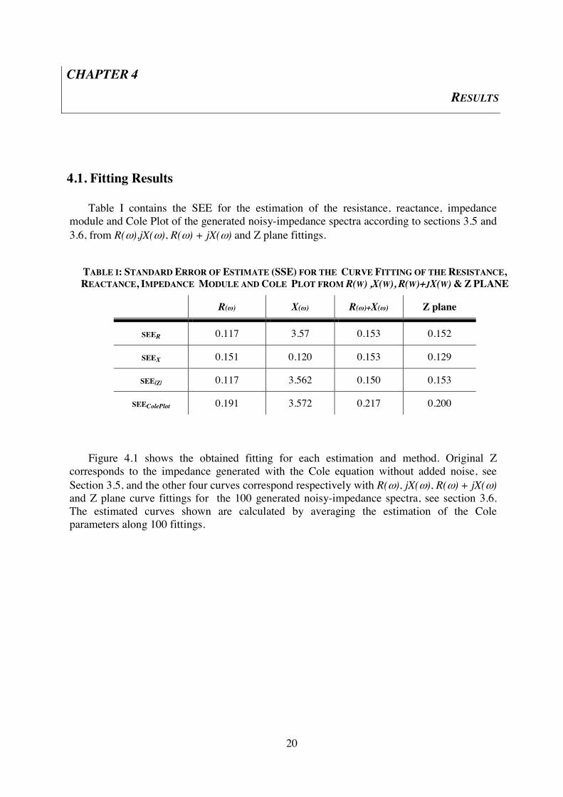
4.1. Fitting Results Table I contains the SEE for the estimation of the resistance, reactance, impedance

module and Cole Plot of the generated noisy-impedance spectra according to sections 3.5 and 3.6, from R(ω),jX(ω), R(ω) + jX(ω) and Z plane fittings.

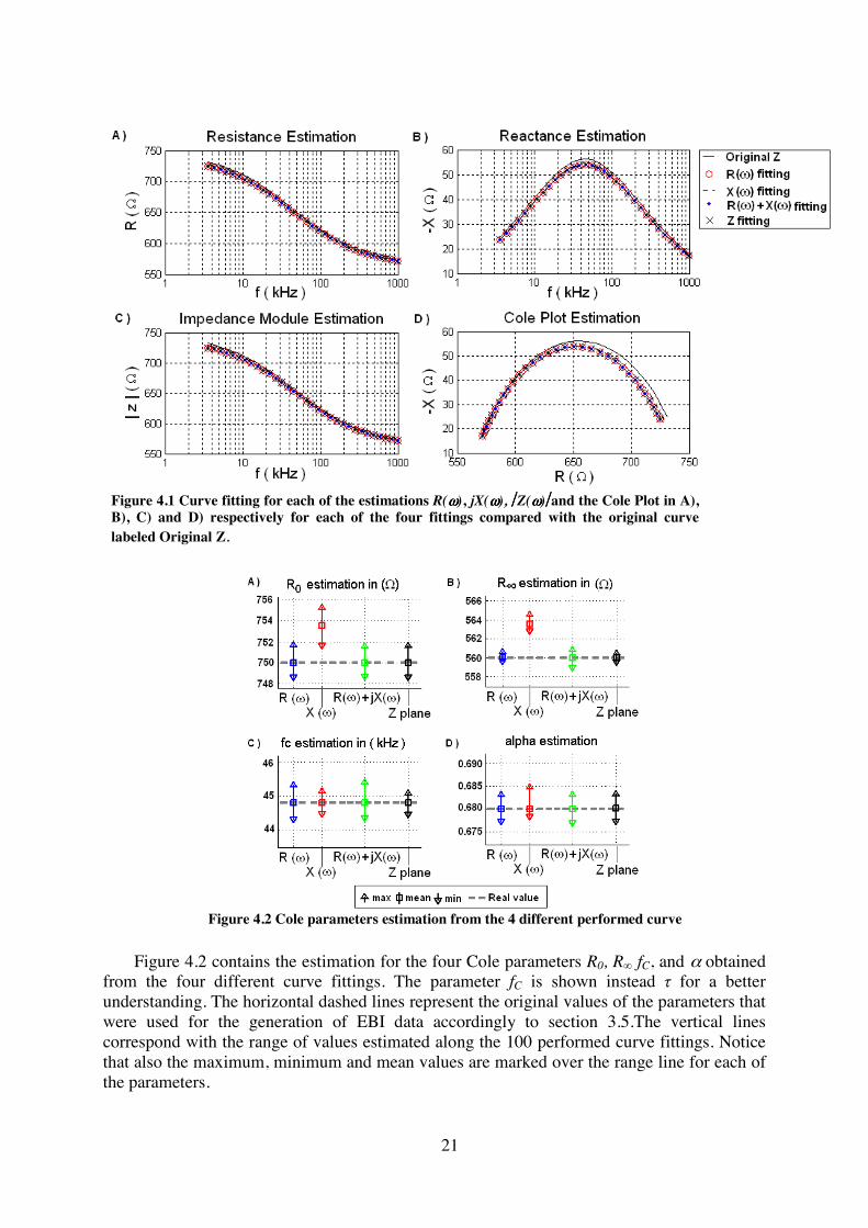
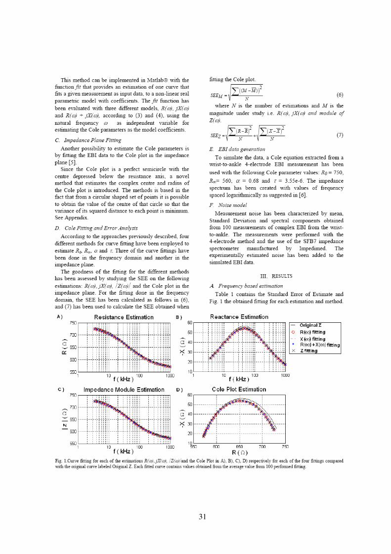
Figure 4.1 shows the obtained fitting for each estimation and method. Original Z

corresponds to the impedance generated with the Cole equation without added noise, see Section 3.5, and the other four curves correspond respectively with R(ω), jX(ω), R(ω) + jX(ω) and Z plane curve fittings for the 100 generated noisy-impedance spectra, see section 3.6. The estimated curves shown are calculated by averaging the estimation of the Cole parameters along 100 fittings.

TABLE I: STANDARD ERROR OF ESTIMATE (SSE) FOR THE CURVE FITTING OF THE RESISTANCE, REACTANCE, IMPEDANCE MODULE AND COLE PLOT FROM R(W) ,X(W), R(W)+JX(W) & Z PLANE

R() X() R()+X() Z plane

SEER 0.117 3.57 0.153 0.152

SEEX 0.151 0.120 0.153 0.129

SEE|Z| 0.117 3.562 0.150 0.153

SEEColePlot 0.191 3.572 0.217 0.200

21

Figure 4.2 contains the estimation for the four Cole parameters R0, R fC, and α obtained

from the four different curve fittings. The parameter fC is shown instead for a better understanding. The horizontal dashed lines represent the original values of the parameters that were used for the generation of EBI data accordingly to section 3.5.The vertical lines correspond with the range of values estimated along the 100 performed curve fittings. Notice that also the maximum, minimum and mean values are marked over the range line for each of the parameters.

Figure 4.2 Cole parameters estimation from the 4 different performed curve

.

Figure 4.1 Curve fitting for each of the estimations R(ωωωω), jX(ωωωω), Z(ωωωω)and the Cole Plot in A), B), C) and D) respectively for each of the four fittings compared with the original curve labeled Original Z.

22

4.2. Frequency Based Estimation Results From Table 1 and Figure 4.1 it is possible to observe that the best fittings for the

resistance spectrum, the impedance module |Z()|, and the Cole Plot are obtained from R(), see Figure 4.1.A), C) & D) respectively, while the best fitting for the reactance spectrum is obtained from X(), see Figure 2.B).

The fitting method using X() performs very badly for all fittings except for the estimation of the reactance spectrum, see Figure 4.1. A), C) & D). When using R() or R() + jX(), the fitting methods performs very well for all the fittings; including the Cole Plot fitting, see Figure 4.1.A), B), C) & D). However, using R() for the fitting of the of reactance spectrum and the Cole fitting, the error is lower than using R() + jX().

4.3. Impedance Plane Estimation Results According to Table 1 and Figure 4.1, the estimation from the impedance plane performs

its best fitting when fit the reactance spectrum and produces the second best fitting of the Cole plot, after R(). For the impedance module |Z(ω)| and the resistance spectrum the obtained fittings provide slightly larger values of SSE than the best obtained curve fittings, so it does not produce the best fitting for any estimation, though all fittings are performed very well.

4.4. Cole Parameters Estimation Results Figure 4.2 indicates that all the fitting methods provide very good estimations for the

Cole parameters, without large errors or trends. It is possible to observe that almost all the mean values of the estimated parameters are close to the original value.

Nevertheless, it is worth commenting some points. Even though the mean of the

estimated values are very close to the real values, the estimation of fC, from R() and R() + jX(), see Figure 4.2.C, present a slightly higher dispersion of values, which results in a maximum deviation just over 1%.

Another important result that can be observed in Figure 4.2.A) & B) is that, the

estimation done from X() for R0 and R is slightly worse than for the rest, what could explains the worse general performance of this method. However the maximum of the observed deviations is still below 0.8%.

4.5. Noise-Error Results The results showed in the previous sections correspond to fittings done to data generated

with experimental noise extracted from real measurements. That is, the noise added to the generated complex impedance spectra in section 3.5 has been produced from experimental measurements. The experimental estimated noise has a real and an imaginary part and each have been added correspondently to the complex impedance spectra. In Figure 3.2 it is possible observe that the value is very small for both the real and the imaginary parts.

In order to study the impact that variations of noise might have in the SEE for the

different curve fittings and estimations of Cole parameter, different levels of noise have been

23

generated just by scaling the experimentally obtained noise. In Figures 4.3, 4.4 and 4.5, the variations of noise are represented in the horizontal axis by the scaling factor values. The value 1 corresponds to the experimental noise level, and each of the values represents a directly proportional linear coefficient from 1 to 30 in intervals of 1.

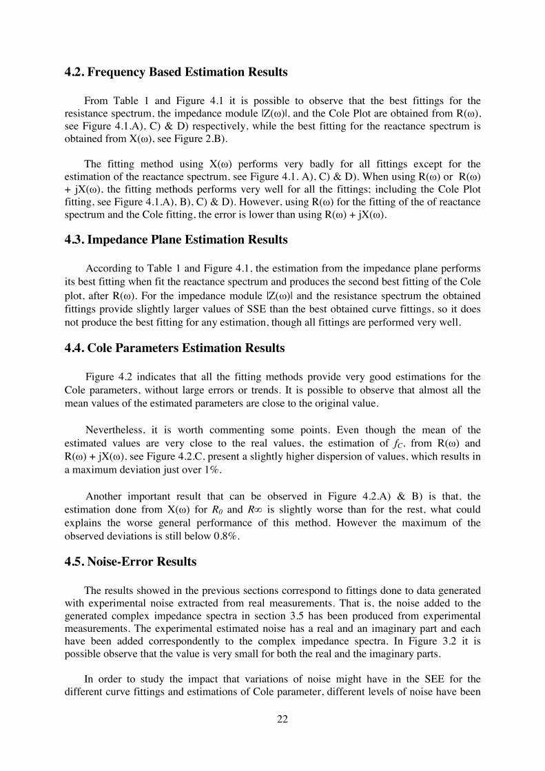
Figure 4.3 shows the variations of the SEE in the estimation of R, X, |Z| and Cole Plot

from R(), X(), R() + X() and Z plane fittings. On Figure 4.3 it can be observed which Curve fitting is more sensible to the added noise in each fitting.

Figure 4.3 Influence of Noise variations on R, X, |Z| and Cole Plot estimations for R (ωωωω), jX(ωωωω), R (ωωωω) + jX (ωωωω) and Z plane fittings in A), B), C) and D) respectively.

24

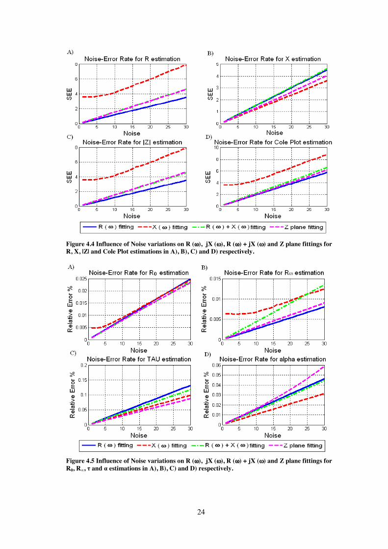
Figure 4.4 Influence of Noise variations on R (ωωωω), jX (ωωωω), R (ωωωω) + jX (ωωωω) and Z plane fittings for R, X, |Z| and Cole Plot estimations in A), B), C) and D) respectively.

Figure 4.5 Influence of Noise variations on R (ωωωω), jX (ωωωω), R (ωωωω) + jX (ωωωω) and Z plane fittings for R0, R, and estimations in A), B), C) and D) respectively.

25

Figure 4.4 shows the variations of the SEE for R (), X (), R () + X () and Z plane fittings in the estimation of R, X, |Z| and Cole Plot. The sensibility to noise variations that each fitting exhibits for each curve fitting can be appreciated on the figure.

Figure 4.5 represents the variations of the SEE for R (), X (), R () + X () and Z plane fittings for the estimation of R0, R, and . That is, it shows the sensibility to noise variations that each fitting has in the estimation of the Cole parameters.

4.6. Noise Influence in R, X, |Z| and Cole Plot Curve Fitting Figures 4.3 and 4.4 report a positive lineal relationship between the obtained SEE and the

Noise variations, as it could be expected. Generally, a method that is better than other with low levels of added noise, keeps the better performance characteristic for increasing levels of noise.

Also, the results show that for a fixed estimation, the fitting that performs the best fitting

for the original noise, continues performing the best when the noise is increasing, even enlarging its difference against the others methods. For instance, in Figure 4.4-A), that shows the estimation of Resistance, it can be appreciated how the SEE of the R () fitting, that was the best with the original noise, increases its difference in performance with the others fittings for increasing level of noise. That means, when noise is increased 30 times, the difference between the SEE of the R () fitting and the SEE obtained with other methods also increases.

Finally, from Figure 4.4 and according to Table I , It can be easily drawn that,

independently of the noise level, the best curve fittings for R, |Z| and Cole plot are done from R () fitting, and for X is done from X () fitting.

4.7. Noise Influence in Cole Parameters Estimation When fitting the curves a positive linear relationship between the obtained SEE and the

level of Noise exists. Generally, the best method to estimate a Cole parameter with low noise is also the best one with higher noise, but sometimes some deviation in the performance of one method occurs. For example, in Figure 4.5-B) it can be observed that with low noise, R is better estimated from R () + X () than from X (), but at high noise levels, X () ends up estimating with less SEE.

Furthermore, observing Figure 4.5 and according to Figure 4.2, we can assert that,

independently of the noise level, the best estimation of R0 is done from the Z plane fitting, the best estimation of R is done from R (); for the best estimation is done from the Z plane fitting, and for the best estimation is done from X () fitting.

26

CHAPTER 5

DISCUSSION

5.1 Methods Performance All the methods considered in this work have performed relatively well for most of the

curve fittings. The exception is the Non-Linear Least Square (NLLS) method that performs very well for the fitting of the reactance using X(), as it could be expected, but this method produces a relatively large SEE for all the rest of the curve fittings.

The slightly lower performance exhibited by the NLLS method when using X() can be

caused by the ability of the method to estimate the Cole parameters R0 and R. Nevertheless the observed differences are exceptionally small.

The exceptional performance of the NLLS method to fit each curve from their corresponding models should not be a surprise due to the non-linear nature of the three models R(ω), jX(ω) and R(ω) + jX(ω).What is more surprising is the observed good performance of the proposed method for fitting curves in the Complex Plane, without making use of the frequency. This relatively good performance is unexpected, especially for the estimation of fC, since we expected that to neglect the frequency information would have more negative impact on the fitting as well as on the estimation of the characteristic frequency.

5.2 Noise Influence The observed relatively good performance of both approaches might be due to the level

of noise used in the fitting. Despite that the noise was modeled from experimental measurements, the obtained noise level was very low. In order to fully evaluate performance of the methods a noise sensitivity test has also been performed. This evaluation depicts a positive linear relationship between SEE and noise for all methods. Furthermore, the results reassert that the method that best perform an estimation with the original noise, keep doing independently of the noise level introduced, even improving its performance comparing the others methods.

5.3 Other Possible Influencing Factors on the Methods Performance

The use of frequencies logarithmically spaced might help to improve the curve fitting as well but this may hold true only for measurement with the characteristic frequency in the lower part of the frequency scale. The distribution of the measurement frequencies in combination with the curve fitting method might have a strong influence on the performance of the curve fitting. To study such relationship is important in order to fully understand the factors influencing the performance of methods for fitting the Cole equation.

Although the EBI data for the curve fittings have been generated from an experimental

biological load like wrist-to-ankle measurements often used for assessment of total body composition and the obtained results can be considered very realistic they conclusions cannot

27

be very generalized until a larger set of fitting data is used, including impedance data extracted from several more EBI applications like, thoracic impedance, segmental limb measurements, cerebral etc.

28

CHAPTER 6

CONCLUSIONS & FUTURE WORK

6.1 General Conclusions On the whole, the studied methods perform relatively well, but the NLLS methods,

especially when fitting on R(ω) and R(ω) + jX(ω), exhibit a superior performance, and above all the R(ω) approach excels. Performing measurements of resistance is quite different than performing measurements of complex impedance and it has important repercussions, especially in the electronic instrumentation of the measurement system. To be able to accurately estimate an equivalent Cole equation for a EBI system from only measurement of resistance would influence significantly several applications of MF-EBI and EBIS that are merely based on the proper estimation of the Cole parameters, like body composition assessment (Kyle, Bosaeus et al. 2004) for instance.

6.2. Future work Since the answer to the question of how many frequencies to use in MF-EBI has been

answered by ward and Cornish (Ward and Cornish 2004), we intend to investigate further the effect of the frequency scaling on the performance of the fitting methods presented in this paper not only to fully validate the NLLS on R(ω) method but also to find the answer to which is the best distribution of frequencies for measuring EBI. In this work, a logarithmic distribution was used, so the results could be generated with a linear distribution, or other distribution, keeping the others conditions, in order to compare the results.

As indicated in the discussion, in order to increase the generalization of the results and

validate their consistency, the fitting should be performed with different types of EBI generated data. The Cole parameters used corresponded with a real wrist-to-ankle 4-electrode measurement, so these parameters can be changed for others values related to another real EBI measurement configuration.

Furthermore, the noise added has been subtracted from a real measurement of a

determined configuration. Noise from other types of measurements can be also proved, or even different methods to model and generate the noise without extracting it from a measurement can be developed.In any case the specific task of characterize properly measurement noise should be addressed specifically.

Another test that would increase the depth of the performance test would be to compare

the curve fitting methods and approaches considered in this study with the curve fitting done by the commercially available software BioiImp from Impedimed.

29

REFERENCES

Aberg, P., I. Nicander, et al. (2004). "Skin cancer identification using multifrequency electrical impedance – A potential screening tool." IEEE Trans. Bio. Med. Eng. 51(12): 2097-2102.

Box, M. J., D. Davies, et al. (1969). "Non-linear optimization techniques". Edinburgh. Cole, K. S. (1940). "Permeability and impermeability of cell membranes for ions" Cold

Spring Harbor Symposia on Quantitative Biology 8: 110-122. Coope, I. D. (1993). "Circle fitting by linear and nonlinear least squares." J. Optim. Theory

Appl. 76(2): 381-388. Cornish, B. H., B. J. Thomas, et al. (1993). "Improved prediction of extracellular and total

body water using impedance loci generated by multiple frequency bioelectrical impedance analysis." Phys. Med. Biol. 38(3): 337-346.

De Lorenzo, A., A. Andreoli, et al. (1997). "Predicting body cell mass with bioimpedance by using theoretical methods: a technological review." Journal of Applied Physiology 82(5): 1542-1558.

Gudivaka, R., D. A. Schoeller, et al. (1999). "Single- and multifrequency models for bioelectrical impedance analysis of body water compartments." Journal of Applied Physiology 87(3): 1087-1096.

Kyle, U. G., I. Bosaeus, et al. (2004). "Bioelectrical impedance analysis--part I: review of principles and methods." Clin Nutr 23(5): 1226-43.

Matthie, J. R., P. O. Withers, et al. (1992). "Development of a commercial complex bio-impedance spectroscopic system for determining intracellular water and extracellular water volumes". Proceedings of 8th International Conference on Electrical Bio-impedance, Kuopio, Finland, University of Kuopio.

Seber, G. A. F. and Wild, C. J. (1989). "Nonlinear Regression. Wiley & Sons Ward, L. C. and B. H. Cornish (2004). "Multiple Frequency Bielectrical Impedance Analysis

how many Frequencies to use?" Proceedings of 12th International Conference on Electrical Bio-impedance, Gdansk, Poland.

"

30

APPENDIX A PAPER CONTRIBUTION TO IEEE-EMBC 2009

The following paper has been produced as result of this thesis work and it has been accepted for publication in the Annual Conference of the Engineering in Biology and Medicine Society hosted by the IEEE in September 2009 in Minneapolis, USA.

31

32

33