Methods for evaluating geometric distortion in magnetic ...

Methods for evaluating geometric distortion in magnetic

resonance imaging

Ville Isokoski

M.Sc. thesisPhysics degree programme

University of Oulu2021

Abstract

Geometric distortions and spatial inaccuracies in magnetic resonance imaging arean important concern especially in image-guided high accuracy operations, suchas radiotherapy or stereotactic surgeries. Geometric distortions in the images arein principle caused by erroneous spatial encoding of the signal echo. Errors inthe spatial encoding are caused by different physical factors, such as static fieldinhomogeneity, gradient field nonlinearities, chemical shift, and magnetic suscep-tibility. The distortion shifts can be quantitatively evaluated as the amount ofdistance or pixels that a signal source has shifted in the mapping from real spaceto the image space. By studying the distortions and the causing mechanisms,corrective measures can be taken to minimize spatial errors in the images.

In this thesis the geometric distortions of one MRI scanner are evaluated withfour different grid phantom objects. The scanner was a 3 Tesla scanner at the OuluUniversity Hospital. The phantoms included two commercial readily availableMRI quality assurance phantoms and two in-house produced prototype phantoms.The methods consisted of imaging the phantoms with different two- and three-dimensional sequences. Image and distortion analysis was performed with onecommercial distortion check software for the respective commercial phantom, andwith an in-house developed Matlab program for all four phantoms.

Results for the magnitude and direction of the distortion as a function of dis-tance from the scanner isocenter were acquired. Three-dimensional distortionshifts up 4 mm within a radius of 200 mm from the isocenter were measured,with occasional shifts up to 9 mm between 100 and 200 mm from the isocen-ter. Distortion field maps and contour plots produced with both analysis methodsseemed to be in accordance with each other, and the geometry and behaviour ofthe field was found to be as expected. As to the prototype phantoms, a result withrespect to the grid density was found. A 5 mm grid separation was too dense withrespect to the achievable resolution for the Matlab analysis script to function, ormore generally for any distortion check at all.

i

Tiivistelmä

Magneettikuvien geometriset vääristymät ja epätarkkuudet ovat tärkeitä huomioonotettavia asioita erityisesti sädehoitoihin tai kirurgisiin operaatioihin liittyvissäkuvantamisissa. Kuvien vääristymät aiheutuvat virheistä signaalien paikkakoodauk-sessa. Paikkakoodaukseen aiheutuu virheitä eri fysikaalisista tekijöistä, kutenstaattisen magneettikentän epähomogeenisuuksista, gradienttikenttien epälin-eaarisuuksista, kemiallisesta siirtymästä tai magneettisesta suskeptibiliteetistä.Geometrinen vääristymä voidaan määrittää kvantitatiivisesti tutkimalla signaalinpaikan siirtymää kuvauksessa todellisesta koordinaatistosta, eli kuvattavasta koh-teesta, kuvan koordinaatistoon. Kuvia voidaan myös korjata vääristymien osaltatutkimalla vääristymien luonnetta ja niiden aiheuttajia.

Tässä tutkielmassa tutkittiin Oulun yliopistollisen sairaalan yhden 3 Teslankenttävoimakkuuden magneettikuvauslaitteen geometrista vääristymää. Kuvauk-sissa käytettiin neljää erilaista fantomia, kahta valmista kaupallisesti saatavillaolevaa sekä kahta kokeellista prototyyppiä. Fantomeita kuvattiin eri kaksi- jakolmiulotteisilla kuvaussekvensseillä. Kuva- ja vääristymäanalyysiä varten käytet-tiin yhtä kaupallista ohjelmaa, joka on tarkoitettu sitä vastaavalle fantomille, sekäitse sairaalassa kehitettyä Matlab-pohjaista ohjelmaa.

Mittausten perusteella saatiin kvantitatiiviset tulokset vääristymän suuru-udelle ja suunnalle, etäisyyden funktiona skannerin keskipisteestä. Kolmiulotteis-ten vääristymien suuruudet olivat 4 mm tai alle 200 mm säteelle asti, suurimpienyksittäisten vääristymien ollessa noin 9 mm tai alle 100 mm ja 200 mm etäisyyksienvälillä. Molemmilla analyysiohjelmilla vääristymien suuntien perusteella luodutvektorikentät olivat toistensa mukaisia ja vääristymän käyttäytyminen vaikuttiodotetulta. Prototyyppifantomien suhteen päädyttiin tulokseen, jonka mukaan5 mm ruudukko oli liian tiheä suhteessa resoluutioon, eikä Matlab-pohjainenanalyysi toiminut. Tarpeeksi leveä ruudukko oli siten oleellinen osa vääristymänmäärittämistä.

ii

Abbreviations

2D Two-dimensional

3D Three-dimensional

ACR American College of Radiology

CIRS Computerized Imaging Reference Systems, Inc.

CT Computed tomography

DBS Deep brain stimulation

FID Free induction decay

FOV Field of view

FT Fourier transform

GE Gradient echo

GTV Gross tumor volume

IR Inversion recovery

MRI Magnetic resonance imaging

NMR Nuclear magnetic resonance

RF Radio frequency

RMS Root mean square

SE Spin echo

SNR Signal-to-noise ratio

SRS Stereotactic radiosurgery

TE Time to echo

TR Time to repetition

iii

Symbols

B0 Static magnetic field flux density

B1 Radio frequency magnetic field flux density

GFE/GR Frequency encoding/readout gradient

GPE Phase encoding gradient

Gx,y,z Gradient in the x, y or z direction

H Magnetic field strength

~ Dirac constant

k Spatial frequency

kB Boltzmann constant

M0 Equilibrium magnetization

Mx,y,z Magnetization in the x, y, or z direction

M⊥ Transverse magnetization

T Temperature

t Time

γ Gyromagnetic ratio

χ Magnetic susceptibility

ω0 Larmor frequency

iv

Contents

Abstract i

Abstract in Finnish ii

List of abbreviations and symbols iii

Contents vi

1 Introduction 1

2 Background 3

2.1 Magnetic resonance imaging . . . . . . . . . . . . . . . . . . . . . . 32.1.1 Nuclear magnetic resonance . . . . . . . . . . . . . . . . . . 32.1.2 Spatial encoding . . . . . . . . . . . . . . . . . . . . . . . . 52.1.3 Pulse sequences and protocols . . . . . . . . . . . . . . . . . 72.1.4 Image resolution . . . . . . . . . . . . . . . . . . . . . . . . 7

2.2 Geometric distortion . . . . . . . . . . . . . . . . . . . . . . . . . . 82.2.1 Sources of geometric distortion . . . . . . . . . . . . . . . . 82.2.2 Distortion characterization and evaluation . . . . . . . . . . 132.2.3 Available correction methods . . . . . . . . . . . . . . . . . . 152.2.4 Quality control and commercial products . . . . . . . . . . . 16

2.3 Need for accuracy . . . . . . . . . . . . . . . . . . . . . . . . . . . . 16

3 Materials and methods 18

3.1 MRI equipment and phantoms . . . . . . . . . . . . . . . . . . . . . 18

v

CONTENTS

3.1.1 3D printed phantoms . . . . . . . . . . . . . . . . . . . . . . 193.1.2 Commercial phantoms . . . . . . . . . . . . . . . . . . . . . 21

3.2 Image acquisition . . . . . . . . . . . . . . . . . . . . . . . . . . . . 233.2.1 3D printed phantoms . . . . . . . . . . . . . . . . . . . . . . 233.2.2 Commercial phantoms . . . . . . . . . . . . . . . . . . . . . 25

3.3 Image analysis . . . . . . . . . . . . . . . . . . . . . . . . . . . . . . 25

4 Results and discussion 27

4.1 3D printed 5 mm grid phantom . . . . . . . . . . . . . . . . . . . . 274.2 3D printed 10 mm grid phantom . . . . . . . . . . . . . . . . . . . . 304.3 The ACR phantom . . . . . . . . . . . . . . . . . . . . . . . . . . . 324.4 The CIRS phantom . . . . . . . . . . . . . . . . . . . . . . . . . . . 354.5 Summary of main results . . . . . . . . . . . . . . . . . . . . . . . . 404.6 Limitations and method comparison . . . . . . . . . . . . . . . . . . 414.7 Possible improvements and future studies . . . . . . . . . . . . . . . 43

5 Conclusions 44

Bibliography 45

vi

Chapter 1

Introduction

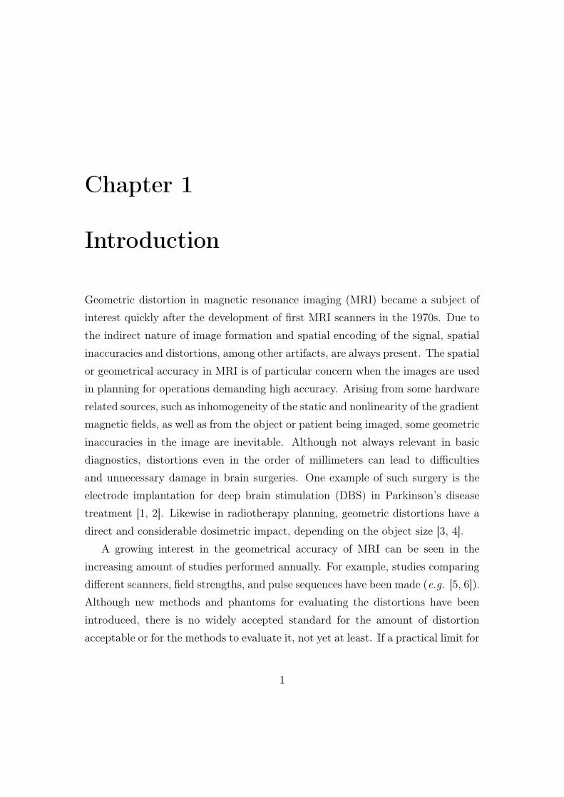
Geometric distortion in magnetic resonance imaging (MRI) became a subject ofinterest quickly after the development of first MRI scanners in the 1970s. Due tothe indirect nature of image formation and spatial encoding of the signal, spatialinaccuracies and distortions, among other artifacts, are always present. The spatialor geometrical accuracy in MRI is of particular concern when the images are usedin planning for operations demanding high accuracy. Arising from some hardwarerelated sources, such as inhomogeneity of the static and nonlinearity of the gradientmagnetic fields, as well as from the object or patient being imaged, some geometricinaccuracies in the image are inevitable. Although not always relevant in basicdiagnostics, distortions even in the order of millimeters can lead to difficultiesand unnecessary damage in brain surgeries. One example of such surgery is theelectrode implantation for deep brain stimulation (DBS) in Parkinson’s diseasetreatment [1, 2]. Likewise in radiotherapy planning, geometric distortions have adirect and considerable dosimetric impact, depending on the object size [3, 4].

A growing interest in the geometrical accuracy of MRI can be seen in theincreasing amount of studies performed annually. For example, studies comparingdifferent scanners, field strengths, and pulse sequences have been made (e.g. [5, 6]).Although new methods and phantoms for evaluating the distortions have beenintroduced, there is no widely accepted standard for the amount of distortionacceptable or for the methods to evaluate it, not yet at least. If a practical limit for

1

CHAPTER 1. INTRODUCTION

the acceptable amount of spatial uncertainty in the images is needed, the accuracylimits concerning, for example, fusion of MRI images with computed tomography(CT) images for radiotherapy planning can be taken as a reference.

The evaluation of geometrical accuracy has been a part of the quality assuranceprograms for some time, but they often lack the proper quantitative methods andcriteria, leaving room for improvement. Also, the distortion correction methodsprovided by the scanner manufacturer, such as passive and active shimming ofthe static field or algorithms in the reconstruction software, which provide sometwo-dimensional (2D) or three-dimensional (3D) distortion correction, succeed inreducing the geometric distortions. However, as not all sources of distortion canbe taken into account quantitatively, some residual error still remains. It can besaid that the task at hand has been concentrated in minimizing the distortionsand developing suitable qualitative and quantitative methods for routine qualityassurance and further studies. [7, 8]

This thesis was done at the Oulu University Hospital with an aim of evaluatingthe residual geometric distortion of selected scanners quantitatively. This includedthe purpose of testing and validating a new 3D printed grid phantom. However,somewhat unexpected intermediate results concerning the grid density led to amore methodological approach. Now, the structure of this thesis consists of abrief look at the background surrounding the subject, followed by methodologicaltesting and quantitative evaluation of the geometric distortion of one 3 T scanner,an essential scanner used for high-accuracy operations planning. The materials andmethods used consist of two readily available commercial phantoms and two in-house 3D printed prototype phantoms, along with a commercial distortion checkprogram and an early stage in-house developed Matlab program. Finally, theresults for all phantoms are discussed comparatively. Some conclusions about theeffect of grid density and the structure of the phantoms are made, along withcomparison of methodological superiority.

2

Chapter 2

Background

In order to gain an understanding of geometric distortion in MRI, it is necessary toestablish an overview of the basic principles of MRI and the causing mechanismsof distortion in the images. In this chapter, the basics of image formation fromnuclear magnetic resonance (NMR) with spatial signal encoding are introducedand the principle causes of distortion are discussed. Adding to the introductorychapter, the need for accuracy in MRI is further discussed along with an overviewof some previous studies.

2.1 Magnetic resonance imaging

2.1.1 Nuclear magnetic resonance

The fundamental basis of nuclear magnetic resonance (NMR) is the behaviourof nuclear spin magnetic moments in an external magnetic field. In NMR ex-periments, the sample under study is placed in an external static magnetic field,B0. This causes the magnetic moments to precess about B0 at the characteristicLarmor frequency

ω0 = γB0, (2.1)

where γ is the gyromagnetic ratio, specific for each nucleus. An external mag-netic field causes the nuclear spin magnetic moments to align into parallel and

3

CHAPTER 2. BACKGROUND

anti-parallel states along B0. A slight difference in the population of these states,which follows the Boltzmann distribution, causes a net macroscopic nuclear mag-netization of the object. In MRI, the 1H nuclei are used to produce the signal,for they are most abundant in water and fat of human tissues. The magnetizationfrom 1H nuclei in a thermal equilibrium is

M0 =ργ2~2B0

4kBT, (2.2)

where ρ is the proton number density, T is the temperature, kB is the Boltzmannconstant and ~ = h/2π is the Dirac constant. In equilibrium, the magnetizationvector

M = M0z (2.3)

is parallel to B0, which is by convention defined to be along the z axis.To produce an NMR signal, a radio frequency (RF) B1 is turned on momen-

tarily to inject energy to the spin ensemble and tip the magnetization from equi-librium towards the transverse plane. The RF pulse frequency is determined bythe Larmor frequency, as to achieve resonance. After absorbing energy from theRF pulse, the spin ensemble seeks to return to its minimum energy, thus emittingthe absorbed energy to the surroundings as RF radiation. The net magnetizationreturns to the equilibrium value parallel to B0. This process is called relaxation.

The relaxation of the transverse and longitudal components of the magnetiza-tion are described by the Bloch equations (see, e.g., [9, 10]). If the magnetizationis initially rotated to the transverse plane, the equations have solutions

M⊥(t) = M0e−t/T2eiω0t (2.4)

Mz(t) = M0

(1− e−t/T1

), (2.5)

or in a rotating frame of reference by simply omitting the oscillating term eiω0t from(2.4). The constants T1 and T2 are the longitudal and transverse relaxation timeconstants. The transverse relaxation is also affected by some local field inhomo-geneities, T ′2, which together with T2 form the total observed transverse relaxation,T ∗2 . The transverse component of the magnetization induces an oscillating voltage

4


in the pickup coil, which is called the free induction decay (FID) signal. The FIDsignal can be expressed as being proportional to

S(t) ∝ S0e−t/T ∗

2 eiω0t, (2.6)

where S0 is the initial signal amplitude at t0, which is proportional to the totaltransverse magnetization in the volume element, or voxel. [10]

In practice, the FID signal decay is quicker than the time needed to properlydetect it. Thus, with a certain method, an echo signal is created and then mea-sured and sampled. The basic types of echoes are the spin echo (SE) and gradientecho (GE) methods. An echo is created when the dephasing of spins due to thetransverse decay is reversed by an RF pulse (SE method) or by switching of thegradients (GE method). The actual pulse sequences and protocols used in MRIare automated and run through by the scanner itself, but they are fundamentallybased on the SE and GE techniques, or a combination of them. [10, 11, 12]

2.1.2 Spatial encoding

Spatial encoding of the NMR signal is the basis for image formation. It is achievedby making the Larmor frequencies depend on their position along an axis in theobject being imaged. This is achieved with the three orthogonal gradient fieldsand their linear combinations that spatially and temporally vary the static field.If a gradient along the x direction is applied, the position along that axis is thenfrequency encoded as

ω(x) = γ(B0 + xGx), (2.7)

whereGx =

∂Bz

∂x(2.8)

is the gradient in the x direction. Similarly,

Gy =∂Bz

∂y(2.9)

andGz =

∂Bz

∂z(2.10)

5


for the y and z directions.For a one-dimensional signal the imaging equation is

S(k) =

∫ρ(x)e−i2πkxdx, (2.11)

where k is the spatial frequency due to the gradient,

k(t) =γ

2π

∫Gx(t)dt. (2.12)

The time dependence thus lies implicitly in the spatial frequencies. For a constantgradient, the spatial frequency is

k =γ

2πGxt. (2.13)

By applying the Fourier transform (FT) to equation (2.11), the effective spindensity as a function of position is recovered, as

ρ(x) =

∫S(k)ei2πkxdx. (2.14)

The above equations can be broadened to 2D and 3D imaging. Generally, thespatial frequency is then

k =γ

2π

∫G(t)dt, (2.15)

where k = (kx, ky, kz) and equation (2.11) can be generalized as

S(k) =

∫ρ(r)e−i2πk·rdr. (2.16)

The 2D or 3D signal is then likewise Fourier transformed to the spatial domain,i.e. the image. [10, 13]

The frequency encoding gradient is more commonly called the readout gradi-ent, GRE or GR, and the frequency encoding direction is thus called the readoutdirection. In 2D and 3D images the other one or two dimensions are phase encodedrespectively. The phase encoding gradients are often denoted as GP .

Slice selection is also done using the gradients. In the beginning of each rep-etition, the slice select gradient is turned on in unison with the RF pulse. Thus,only the spins within the selected slice are excited. The slice thickness is affectedby the applied gradient strength and the bandwidth of the RF pulse, which is therange of frequencies contained in the pulse.

6


2.1.3 Pulse sequences and protocols

During MRI image acquisition, pulse sequences consisting of RF and gradientpulses are applied and the signal is sampled discretely. The sampled data is col-lected to the acquisition matrix, or k-space, which represents the image in thefrequency domain and consists of the spatial frequencies, which then via the in-verse FT form the final image. The filling of k-space can be done in various ways,as the k-space trajectory is determined only by the applied gradients, as in equa-tion (2.15). For example, cartesian, radial, or even spiral sampling methods exist,each having their own advantages and disadvantages. [13, 14, 15]

Each sequence and clinical protocol is usually designed for some specific purposeand usually some compromises have to be taken into account. For example, theBLADE technique is commonly used for motion artifact reduction (e.g. [14]). Ituses radial k-space sampling, such that the center of k-space is oversampled. As thelow spatial frequencies, i.e. contrast, are oversampled and then interpolated, somespatial accuracy is always lost in return. On the other hand, protocols used fore.g. radiotherapy planning are designed such that the imaging time is increasedand some signal-to-noise ratio (SNR) is lost to maintain resolution and spatialaccuracy.

2.1.4 Image resolution

The spatial resolution in MRI is defined as the size of the voxels. It thus relatesto the size of the field-of-view (FOV), slice thickness, and the acquisition matrix.Similarly in 3D imaging, where the slice thickness is ”replaced” by the secondphase encoded dimension. Unless the voxels are isotropic, the in-plane resolutionis perceived differently depending on the viewing direction. Also, reducing thevoxel size enhances the resolution, but the voxel signal strength and SNR arealways reduced as a trade-off. This can be compensated, e.g., by adding thenumber of averages, which in turn is seen as an increase in the imaging time. [10]

7


2.2 Geometric distortion

2.2.1 Sources of geometric distortion

To understand the geometric distortion of an MR image, it is necessary to establishan overview of the causing mechanisms. At the principle level, geometric distortioncan be said to be the mismapping of spins, or a shift in the apparent location of asignal echo. This can happen due to various known reasons.

The sources that cause distortion can be divided to so called hardware relatedand object related sources, or sequence dependent and independent sources. Thehardware related sources arise from the scanner itself and include the static fieldinhomogeneities and gradient nonlinearities. The object related sources arise fromthe patient or subject being imaged and include the magnetic susceptibility andchemical shift induced distortions.

It should be noted that, as stated in multiple studies, geometric distortionis inherently 3D in a sense that the in-plane distortion is also affected by spinsoutside the slice. Therefore, attention should be paid when trying to assess thetrue 3D distortion from 2D images. [5, 16]

Static field inhomogeneities

Most modern MRI scanners are closed bore, or cylindrical type, where the staticmagnetic field is created with superconducting coils. Static field inhomogeneitiesarise from the properties and design compromises of the coils and are one of themain reasons for distortion in the images. Spatial encoding of the signal relies ona homogenous static B0 field, which the linear gradients then modulate creatingspatial frequencies. Thus, any non-uniformity of the static field or any deviationfrom gradient linearity distorts the spatial frequencies, resulting in distortion inthe image. [7]

The static field is purely homogenous only in theory. In reality, near-homogeneity is achieved only within a certain spherical imaging volume aroundthe scanner isocenter. The homogeneity within this volume is usually within afew parts-per-million (ppm). [17]

8


The static field homogeneity is enhanced by so called passive and active shim-ming. Passive shimming gives a robust ’zeroth order’ correction, reducing theinhomogeneity by a certain amount. It is commonly done manually, e.g. withmetal plates fixed inside the scanner bore. As the static field strength decays withtime, the passive shims need to be adjusted from time to time, which is a timeconsuming process. [10, 18]

Active shimming however, is more advanced, as it uses shimming coils forcorrecting the homogeneity. With the active shimming coils, real time correctionscan be made to the field homogeneity. As every object and patient being imageddisturbs the static field, real time corrections are often required and in fact, asa part of the pre-scan routine, the scanner goes through a shimming sequence inorder to make sure, that the best possible field homogeneity is achieved. The staticfield inhomogeneities are sequence dependent, so attention should be paid whenassessing the distortion with different protocols and sequences. [10, 19]

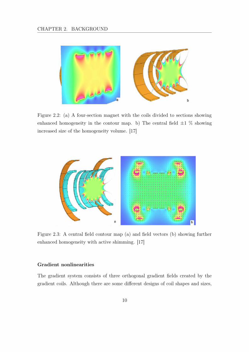
In the figures 2.1 - 2.3, taken from Overweg (2008) [17], the relation of enhancedhomogeneity to the size of the acceptable imaging volume is clearly shown.

Figure 2.1: a) Field vectors of the static field in a solenoidal magnet. b) A contourmap of the static field uniformity. c) Contour map of the central field with a ±1% deviation in homogeneity, showing a volume of homogeneity not nearly largeenough for imaging.[17]

9


Figure 2.2: (a) A four-section magnet with the coils divided to sections showingenhanced homogeneity in the contour map. b) The central field ±1 % showingincreased size of the homogeneity volume. [17]

Figure 2.3: A central field contour map (a) and field vectors (b) showing furtherenhanced homogeneity with active shimming. [17]

Gradient nonlinearities

The gradient system consists of three orthogonal gradient fields created by thegradient coils. Although there are some different designs of coil shapes and sizes,

10


the main purpose of producing linearly varying gradient fields for spatial encoding,is the same.

Figure 2.4: A simplified idea of gradient linearity. The linearity around the isocen-ter in the certain volume is acceptable, but degrades with distance from the isocen-ter. [20]

The gradient coils mostly produce nearly linear orthogonal modulations of thestatic field within a certain linearity volume around the isocenter, but as with staticfield homogeneity, perfection is only achieved in theory. Near perfect linearitywould be achievable, but practical requirements often lead to design compromises.For example, the need for very short gradient field rise times dictate the coil designby a certain degree, at the cost of maintaining linearity. On the other hand,stronger gradients and rapid switching times induce eddy currents, which have anaffect on the static field homogeneity. Also, some physiological concerns arise, suchas possible peripheral nerve stimulation and loud acoustic noise. As with staticfield inhomogeneities, the gradient nonlinearities increase rapidly with distancefrom the isocenter. For a given scanner, the gradient nonlinearity distortions aresequence-independent. [19, 21, 22]

Magnetic susceptibility

In addition to the hardware related sources, there are also some object or patientrelated factors causing distortion in the images. Every object interacts with themagnetic field it is placed in, the magnitude of the interaction depending on its

11


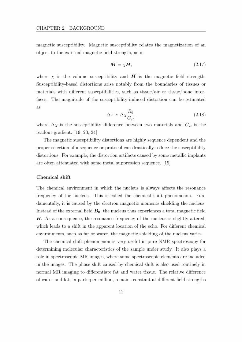
magnetic susceptibility. Magnetic susceptibility relates the magnetization of anobject to the external magnetic field strength, as in

M = χH , (2.17)

where χ is the volume susceptibility and H is the magnetic field strength.Susceptibility-based distortions arise notably from the boundaries of tissues ormaterials with different susceptibilities, such as tissue/air or tissue/bone inter-faces. The magnitude of the susceptibility-induced distortion can be estimatedas

∆x ' ∆χB0

GR

, (2.18)

where ∆χ is the susceptibility difference between two materials and GR is thereadout gradient. [19, 23, 24]

The magnetic susceptibility distortions are highly sequence dependent and theproper selection of a sequence or protocol can drastically reduce the susceptibilitydistortions. For example, the distortion artifacts caused by some metallic implantsare often attenuated with some metal suppression sequence. [19]

Chemical shift

The chemical environment in which the nucleus is always affects the resonancefrequency of the nucleus. This is called the chemical shift phenomenon. Fun-damentally, it is caused by the electron magnetic moments shielding the nucleus.Instead of the external field B0, the nucleus thus experiences a total magnetic fieldB. As a consequence, the resonance frequency of the nucleus is slightly altered,which leads to a shift in the apparent location of the echo. For different chemicalenvironments, such as fat or water, the magnetic shielding of the nucleus varies.

The chemical shift phenomenon is very useful in pure NMR spectroscopy fordetermining molecular characteristics of the sample under study. It also plays arole in spectroscopic MR images, where some spectroscopic elements are includedin the images. The phase shift caused by chemical shift is also used routinely innormal MR imaging to differentiate fat and water tissue. The relative differenceof water and fat, in parts-per-million, remains constant at different field strengths

12


and it can also be stated as a difference in frequency at different fields. Thus, it isdirectly transferable to pixels, making it a highly usable and reliable method.

Despite its advantages, the resultant distortion or apparent spatial shift re-mains existent in the images even when it needs not to. Like the static fieldinhomogeneities and magnetic susceptibility, chemical shift is also highly sequencedependent. It is manifested in the frequency encoding direction for SE and GREsequences and may also appear in the phase encoding direction for the echo planarimaging (EPI) technique. [19, 25]

2.2.2 Distortion characterization and evaluation

Direct techniques

Geometric distortion can be defined as the spatial error or difference between thereal dimensions in the object and the corresponding dimensions in the image. Forexample, the distance between two known and well defined points in the imageshould accurately correspond to the equivalent distance in the patient or a phan-tom. The 3D geometric distortion can be characterized by the positional errors

dx(x, y, z) = x′(x, y, z)− x (2.19)

dy(x, y, z) = y′(x, y, z)− y (2.20)

dz(x, y, z) = z′(x, y, z)− z, (2.21)

where x′, y′ and z′ are coordinates in the distorted space (i.e. the image) and x, y,and z are the real space coordinates. The distance in 3D space can then be simplyexpressed with Euclidean metrics

dr =√dx2 + dy2 + dz2. (2.22)

The real dimensions can be determined from the object itself, but this is of courseonly reliable for a phantom object consisting of, for example, a well known gridstructure. [16]

Another method is to use CT images as a reference. For all practical purposes,CT images can be thought of as geometrically accurate, as the imaging technique

13


is in a way more straight forward compared to MRI. When compared to CT, thegeometric distortion can be expressed as

dx = dxMRI − dxCT (2.23)

dy = dyMRI − dyCT (2.24)

dz = dzMRI − dzCT (2.25)

or simplydi = iMRI − iCT , (2.26)

where i = x, y, z. The 3D distance can then be similarly evaluated as in (2.22).Calculating the difference between distorted and non-distorted points is rather

straight forward, but the methods used for control point identification and extrac-tion are underscored and vary from study to another.

Indirect techniques

In addition to the direct phantom techniques, there are also some indirect tech-niques for evaluating and correcting the distortion. One such technique is toacquire two sets of images with the same sequence but different readout gradi-ent polarities. The sequence-dependent distortions are sensitive to this change ingradient polarity, leading to a difference in apparent control point positions. Bycomparing these differences, the sequence-dependent distortions can be attainedand mitigated. [19]

For example, in a 2017 study by Weavers et al. [26], the gradient non-linearityfields were studied using reversed polarity gradients. A large phantom containingsmall water-filled spheres was scanned with increased receiver bandwidth and twoacquisitions with reversed gradient polarities, in order to mitigate the systematicoff-resonance errors. By comparing the apparent shifts of the control points to aCT ’truth’, the sequence-independent distortions could be attained. By iterativemethods, the spherical harmonic coefficients of the gradient fields could then beestimated. The results suggested that even more accurate calibrations to the gra-dient non-linearity coefficients could be made, compared to the vendor corrections.[26]

14


2.2.3 Available correction methods

Some methods for distortion correction due to gradient nonlinearities were devel-oped already in the 1980s [8]. Nowadays, after each sequence is acquired, the rawimages are automatically filtered and corrected for some amount of distortion. Foreach image, a pre-determined 2D or 3D distortion correction algorithm is applied,reducing the geometrical inaccuracies. The correction methods are built in to thesoftware and accessible to the user only such that they can be turned on or off fora particular sequence. All other software and parameters remain hidden. Theyutilize the direct and indirect methods discussed in the previous section, such asdistortion maps calculated with the displacement errors or phase error maps cre-ated with the different readout gradient polarities. For at least the 3D correction,the scanners use some real time shimming data. Also, in some studies during therecent years, some novel distortion correction algorithms have been developed.

The correction algorithms enhance the geometrical and spatial accuracy, butnot all factors can be mitigated. Some distortion is thus always present even aftercorrection. This is called residual distortion or residual error.

Figure 2.5: Magnitude of original distortion in an uncorrected image (left) andresidual distortion after correction (right). [27]

15


In figure 2.5, taken from a study by Baldwin et al. [27], the magnitude ofdistortion in the transversal plane can be seen uncorrected (left) and corrected(right). It is clearly seen that the correction algorithm succeeds well in reducing thedistortion, but not completely. Some residual error in the order of sub-millimeterremains, which is nonetheless acceptable for high accuracy demands.

2.2.4 Quality control and commercial products

The evaluation of geometric distortion is an essential part of existing MRI qualitycontrol and assurance programs. For example, the American College of Radi-ology (ACR) MRI accreditation program provides a multipurpose phantom forroutine quality control, including testing 2D in-plane geometrical accuracy. An-other commercial provider is the Computerized Imaging Reference Systems, Inc.company (CIRS), which designs, develops, and manufactures phantoms for allimaging modalities. For MRI there are, for example, the large field MRI distor-tion phantom, the MRI distortion phantom for stereotactic radiosurgery (SRS),and a distortion check software for automated image analysis.

2.3 Need for accuracy

Spatial and geometrical accuracy and reliability is an important aspect when us-ing MRI for high precision means, such as radiotherapy planning or stereotacticsurgery guidance. For example, geometric distortions in image-based radiother-apy planning have a direct and considerable dosimetric effect, as stated earlier.Geometric inaccuracies in excess of a few millimeters are already a concern, asunnecessary radiation dose should be avoided. [3, 19]

For neurosurgical applications, such as biopsy or electrode implantation, bestachievable geometrical accuracy of the images is highly desirable, and even smallinaccuracies may cause unnecessary damage during the operations. As shown bysome previous studies, the in-plane geometric distortion as a function of distancefrom the scanner isocenter increases rapidly, reaching magnitudes of 5-10 mm

16


even within relatively short distances from the isocenter. A magnitude of thedistortion over 5 mm at a distance of 15 cm from the isocenter means that evenwithin imaging volumes the size of the brain, notable distortions may have to betaken into consideration. Furthermore, in head imaging the center of the head israrely located precisely at the isocenter. This can cause a pronounced difficultyfor example in radiotherapy or surgery of the back of the skull. [1, 7]

For example, in a 2016 paper by Seibert et al. [28], 28 stereotactic radiosurgerycases were studied retrospectively, as it is highly dependent on accurate imageguidance. A 3D correction algorithm for the gradient nonlinearities was applied tothe images and the gross tumor volumes (GTV) in the corrected and uncorrectedimages were compared. The dose planning was done with the uncorrected images,but the actual received dose was measured with the GTVs in the corrected images.The results showed a median displacement of 1.2 mm of the GTV, minimum being0 mm and maximum being 3.9 mm, leading to some cases fulfilling the criteria of ageometric miss. The conclusions were in accordance with previous studies, statingthat although the geometric distortions in MRI are subtle and difficult to assessvisually, the clinical impact of the distortions is significant.

17

Chapter 3

Materials and methods

In this chapter the phantom objects and the MRI scanner used are introduced.The properties and purpose, and the image acquisition process for each phantomare explained. The used image processing and analysis methods are specified.

3.1 MRI equipment and phantoms

The images for this thesis were acquired with a 3 T MRI scanner and with a totalof four different phantoms, at the Oulu University Hospital. The scanner is usedin routine diagnostic imaging, and for radiotherapy and high accuracy surgicalplanning. Some technical properties of the scanner are listed below.

Table 3.1: Some technical properties of the scanner.

Scanner Static field Max. rms gradient Max. rms slew Dimensions(T) strength (mT/m) rate (T/m/s) (cm) × (cm)

Siemens Vida 2.9 60 200 70 × 186

18

CHAPTER 3. MATERIALS AND METHODS

3.1.1 3D printed phantoms

Two prototype phantoms were previously produced with a 3D printer, with theaim of testing a novel 3D distortion grid phantom which would be suitable tobe used with the head coil. The printer was an Objet30 Prime (Stratasys, Ltd.)printer. According to the manufacturer, the printing accuracy is 0.1 mm with aminimum layer thickness of 16 µm. The printing was done using a bio-compatible,MED610, material, a Windows 3D builder program, and an open-source Matlablattice generator program for the grids. For details of the printer, materials, orthe Matlab program, see [29, 30, 31].

The 3D printed 5 mm grid phantom (figure 3.1) consists of a cylinder andtwo grids (figure 3.2) fitted inside. The cylinder is filled with paraffin oil forsignal generation. The grid thickness is 1 mm with an equal 5 mm spacing in alldirections.

Another smaller 3D printed phantom prototype was a 3D printed grid inside anormal canister (figure 3.3) The grid is similar to the 5 mm grid, but considerablysmaller and with a sparser 10 mm spacing. Paraffin oil was likewise used for signalgeneration. It should be noted, that this prototype was really a rather rudimentarypiece for testing the effect of the increased grid spacing from 5 mm to 10 mm.

19


Figure 3.1: The 3D printed cylinder.

Figure 3.2: A sample piece of the 3D printed 5 mm grid.

20


Figure 3.3: The prototype 10 mm grid inside a canister.

3.1.2 Commercial phantoms

In addition to the two 3D printed prototype phantoms, two commercial phantoms,the CIRS large field distortion phantom and the ACR phantom, were used.

The CIRS large field MRI distortion phantom (from now on, the CIRS phan-tom) is designed for routine assessment of 3D distortion caused by the nonlinearmagnetic field. The phantom (figure 3.4) consists of a plexiglass cylinder, whichcontains an orthogonal 3D grid inside the volume. The cylinder is 300 mm inlength, 276 mm in height, and 330 mm in diameter. The grid consists of plasticrods 3 mm in diameter, spaced 20 mm apart. The cylinder can be filled with asignal-generating solution, such as water or paraffin oil, although when filled withwater, imaging in a 3 T field produces strong dielectric artifacts (e.g. [32]). Itcan be also be emptied for CT imaging, in which the grid/air interface providesgood contrast. For purposes of this thesis, the cylinder was filled with paraffin oil,essentially to avoid dielectric artifacts.

21


Figure 3.4: The CIRS large field distortion phantom.

Another commercial phantom, the ACR phantom (figure 3.5), is a closed acrylicplastic cylinder, with an inside length of 148 mm and inside diameter of 190 mm.The cylinder is filled with a mixture of NiCl2 and NaCl for signal generation. Insidethe cylinder are multiple structures for a variety of scanner performance tests, suchas central frequency, transmitter gain or attenuation, and spatial resolution. Fortesting the geometric accuracy there is a sparse grid, which by itself is only meant tobe visually inspected from the images, but it can also be used as means of locatinga few control points. As the phantom is a multipurpose one, the grid meant forgeometric accuracy assessment is only a 2D grid. This is a limitation, because ofthe 3D nature of the distortion, and it will be discussed later. Also, if images frommultiple orientations need to be acquired and compared, the phantom needs tobe repositioned on the table, which means degraded reliability and comparability.[33]

22


Figure 3.5: The ACR MRI phantom. The distortion grid is visible in the middle.

3.2 Image acquisition

3.2.1 3D printed phantoms

Images of the 3D printed grid phantoms were acquired using a 64-channel headcoil and two different 3D sequences. The two sequences, MPRAGE and SPACE,were chosen on the basis that they are commonly used 3D volume sequences forhigh resolution isotropic head imaging. The MPRAGE sequence is essentially aT1-weighted 3D rapid gradient echo sequence added with an inversion recovery(IR) pulse for better contrast, whereas the SPACE sequence is a T2-weighted 3Dfast spin echo sequence with very short echo times and long echo train lengths.

23


3D printed 5 mm grid phantom

With this phantom, images from all three principle directions were acquired withboth sequences. One of the original aims was to test the effect of slice orientationand sequence to the amount of distortion. In addition, one transversal slab withMPRAGE was acquired with the body coil for possible comparison of the receivingcoil.

For both sequences an acquisition matrix of 512 x 512, FOV 256 mm x 256mm, and slice thickness of 0.50 mm were chosen, giving an isotropic voxel size of0.50 × 0.50 × 0.50 mm3. The grid thickness is 1.0 mm, so the isotropic voxel sizeneeded to be small enough for the resolution to suffice for feature extraction. Abetter resolution would have been beneficial, but technical matters in the sequencedesign limited the acquisition matrix size giving the in-plane resolution of 0.50 mm.Also, the SNR becomes a concern with decreasing voxel sizes and the number ofaverages would have to be increased to maintain the SNR, leading to unreasonablylong imaging times.

The slices from all directions were then reformatted to the transversal orien-tation for comparability and also to align the slices more accurately with the gridstructure of the phantom.

3D printed 10 mm grid phantom

Similar to the 5 mm grid, the 10 mm grid was also imaged with a 64-channelhead coil and with the MPRAGE and SPACE sequences. Unlike the 5 mm grid,only the transversal slabs were acquired, with two different resolutions for bothsequences. The same FOV of 256 mm x 256 mm was chosen, with two differentacquisition matrix sizes of 256 x 256 and 512 x 512, with a slice thickness of 1.0mm and 0.5 mm respectively. Thus, the voxel sizes were once again isotropic 1.0x 1.0 x 1.0 mm3 and 0.5 x 0.5 x 0.5 mm3.

24


3.2.2 Commercial phantoms

ACR phantom

For the ACR phantom, a large FOV geometric distortion quality assurance methodby Siemens was used [34]. The phantom was placed upwards on the scannertable, such that the grid structure (fig. 3.5) was oriented in the coronal direction.Then, the grid was imaged with the body coil and a high resolution 2D spinecho sequence with 550 x 550 mm FOV, 512 x 512 acquisition matrix and slicethickness of 5 mm. The scanner table was programmed for automatic movementbetween sequences such that five coronal images with the same FOV but differentgrid position were acquired. This was repeated with different phantom positionsalong the x-direction. The images were then added together using an arithmeticmean function, a property of the scanner software. This way, the resulting imageconsisted of the grid structure filling a large FOV and visible distortion at theedges (see results).

CIRS large field phantom

The images of the CIRS large field phantom were acquired in collaboration withthe department of radiation therapy, for their own quality control purposes. Thephantom was placed on the scanner table as in fig. 3.4, using the body and spinecoils as receiving coils. The selected images used in this thesis are coronal slicesacquired with a 2D turbo spin echo sequence. The slice thickness was 0.9766 mmand a FOV of 500 mm x 500 mm and a 512 x 512 acquisition matrix gave theresolution of 1.0240 pixels per mm.

3.3 Image analysis

For image analysis, two different tools were used. One, meant to be used with allphantoms, was an in-house Matlab program. The program was made previouslyfor upcoming studies and testing of the 3D printed prototype phantoms. The corepurpose of the script is to take an image of a grid, extract the rod intersection

25


points, compare them with a non-distorted ”true” lattice, and return the differenceof the points in pixels as well as the direction of the point shifts. Starting fromthe middle of the image, the central horizontal and vertical rods are found usingthe corresponding horizontal and vertical grayscale profiles, in which the localminima represent the smallest grayscale values, i.e. the rods. Beginning from thecenter, each rod found are traced separately in each direction, combining theminto lateral and vertical sequences of points. These sequences are then smoothedwith polynomial interpolation, such that the effect of the ratio of resolution torod thickness would be less emphasized. From these smoothed point sequences,the grid intersection coordinates are then extracted. Finally, the intersection pointclosest to the center of the image is chosen, and an ideal non-distorted point latticeis generated according to a known preset grid distance. The difference in pixelsbetween the corresponding non-distorted and distorted points are then calculated,as in section 2.2.2.

Another analysis software used was the CIRS distortion check program, anonline cloud-based application meant to be used for the CIRS phantoms. It fea-tures fully automated detection of all grid intersections and control points forcomparison with a CT ’truth’. After interpolation, 3D distortion vector fields aregenerated. The resulting distortion fields can be reported for example as scatterplots or contour plots. [35]

Additionally, an open-source image processing program ImageJ was used forimage viewing and plotting some rudimentary line intensity profiles, which will beseen in the next chapter.

26

Chapter 4

Results and discussion

In this chapter the relevant images and subsequent analysis are presented, alongwith simultaneous discussion and notices. Some main limitations are emphasized,along with some comparison of the different methods and results. Finally, possibleimprovements and future studies are briefly discussed.

4.1 3D printed 5 mm grid phantom

The 5 mm grid prototype phantom was imaged with different sequences, coils andorientations with a variety of things in mind. In figures 4.1a and 4.1b, two slicesof the transversal MPRAGE slab are shown. The images are precise and the goodamount of averages gives great SNR and contrast despite the small voxel size.Rather surprisingly however, the Matlab script was unable to produce sensibleresults. There were always, for example, some point sequences not finding thelocal minima and the middle of the rod, which was a fundamental difficulty. Thereason traces to the ratio of resolution to the grid dimensions, especially the roddistances. To illustrate, in figures 4.2 - 4.4, the grey value intensity profiles areplotted from two different positions. In figure 4.3, the effect of the grid being toodense is shown. The local minima and maxima are too close to each other and asderivatives of the profile are also used, problems arise. On the other hand, as seenin figure 4.4, the local minima are almost indistinguishable from the base line.

27

CHAPTER 4. RESULTS AND DISCUSSION

(a) (b)

Figure 4.1: Transversal MPRAGE images of the 5 mm grid phantom with oneslice from between the rods (a) and one including the in-plane rods (b).

(a) (b)

Figure 4.2: Positions which the intensity profiles in figures 4.3 and 4.4 are plottedalong, shown by the yellow lines.

28


Figure 4.3: Grey value intensity profile for fig. 4.2a.

Figure 4.4: Grey value intensity profile for fig. 4.2b.

29


4.2 3D printed 10 mm grid phantom

The images of the 10 mm grid phantom were not taken through the Matlab pro-gram, but preliminary results were more promising, as for the grid density and theintensity profiles. In figures 4.5a and 4.5b, the higher resolution images of bothsequences are shown. As is clearly seen, widening the grid spacing from 5 mm to10 mm makes a remarkable difference. The intensity profiles are again plotted forboth along the yellow lines shown. The profiles for 4.5a and 4.5b are shown infigures 4.6 and 4.7 respectively. Now, the local minima are clearly distinguishable.The rods are thin enough and far apart to be distinguishable even with lower reso-lution. Unlike with the 5 mm grid, the ratio of grid density to resolution is not somuch of a concern here. It should be noted, that the apparent grid warping in bothimages is not due to geometric distortion, but simply because of the interaction ofthe grid material with the filling oil. This is, again, one more problem of a kindand will be discussed further.

(a) (b)

Figure 4.5: Transversal MPRAGE (a) and SPACE (b) images of the 10 mm gridphantom.

30


Figure 4.6: Intensity profile of the MPRAGE image, plotted along the yellow linein figure 4.5 (a).

Figure 4.7: Intensity profile of the SPACE image, plotted along the yellow line infigure 4.5 (b).

31


4.3 The ACR phantom

Images of the ACR phantom were analyzed with the Matlab script and the resultscan be seen in figures 4.8 - 4.11. In figure 4.8, the vertical and horizontal pointsequence and polynomial interpolation curves are shown. As can be seen, the areasaround the center of the image are rather immaculate, but at the edges and morefaded areas, problems occur.

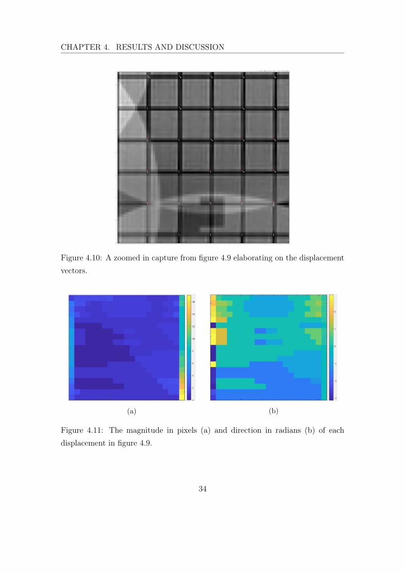
In figure 4.9, the displacement vectors for almost each control point are shown.The residual geometric distortion manifests itself clearly at the top and the bottomas the warping of the grids. The most outward left and right columns of pointsshould be neglected, as they are miscalculated (shown also in figure 4.8). Atthe center of the image the distortion is practically non-visible and growing inmagnitude towards the edges, as it of course should be, based on our existingknowledge. Due to the large FOV in figure 4.9, the displacement vectors are onlyclearly distinguishable when ’zoomed in’, as in figure 4.10. The distortion shiftsare in the order of one to two pixels, which, estimated from the resolution, accountto an order of one to two millimeters in magnitude of the residual distortion.

Finally, the magnitude of the distortion for each point is shown in figure 4.11aand the relative direction of the shift in radians in figure 4.11b, with the respectivecolor codings. Although the grid covers a relatively large FOV in the coronal plane,the magnitude of the distortion remains rather moderate. Only at the edges, visibledistortion and warping of the grids can be seen. On the other hand, those areas arenot covered by the algorithm. Additionally, it should be once again emphasized,that only the 2D in-plane distortion can be evaluated. This means, in essence,that even though a pixel could be shifted in the sagittal plane, only a projectionto the coronal plane of the total shift is seen. If a better understanding is wanted,the phantom needs to be imaged from all directions and at different heights inorder to form even a decent picture of the 3D distortion field.

32


Figure 4.8: The horizontal and vertical line finding point sequences and polynomialinterpolation curves.

Figure 4.9: The displacement vectors for each recognized intersection point.

33


Figure 4.10: A zoomed in capture from figure 4.9 elaborating on the displacementvectors.

(a) (b)

Figure 4.11: The magnitude in pixels (a) and direction in radians (b) of eachdisplacement in figure 4.9.

34


4.4 The CIRS phantom

The CIRS phantom images were analyzed with two different tools, the Matlabprogram and the CIRS distortion check software. Thus, some comparability andcross check could be done. As to the Matlab program, in the coronal image infigure 4.12, the line finding curves are seen, along with the distortion manifestedas warping at the edges. Except for the bottom row and the rightmost column,the grid is recognized properly. In figure 4.13, the displacement vector field isseen. Now, even with a large FOV image, the distortion shifts can be clearly seen.The distortion is negligible at the center of the image, but once again growing inmagnitude towards the edges, as expected. Likewise, in figure 4.14a, the magnitudeof distortion in pixels is shown, along with the direction of the shift in radians infigure 4.14b. In both 4.13 and 4.14b, the change of direction in the shift is shown.

Figure 4.12: The line finding curves for the CIRS phantom.

35


Figure 4.13: The displacement vector field.

(a) (b)

Figure 4.14: The displacement magnitudes in pixels (a) and direction in radians(b) for each control point.

36


The CIRS distortion check software provided a full analysis report containingbasic data acquisition information, contour plots for all three principal orientations,scatter plots, and error tables. From these, a few selected figures are shown here.In figure 4.15, a coronal contour plot of the distortion magnitude is shown. Thesudden increase in the distortion magnitude at large z values, i.e. the top of theplot, is due to shielding plates of the scanner room wall, close to the opening ofthe scanner bore. A comparison between figures 4.14a and 4.15 is not facile, butsome similarities at least in the order of magnitude can be pointed out, such asthe distortion growing in magnitude from the center towards the edges and theamount of distortion being in the order of 1 to 2 pixels or 1 to 3 millimeters.

Figure 4.15: Coronal contour plot.

37


Figure 4.16: Sagittal contour plot.

In figure 4.16, the sagittal contour plot is shown. The shape of the distortionfield and the resemblance with the static field homogeneity contour plot in figure2.3 is notable. The effect of the scanner room shielding plates can be seen, similarto figure 4.15. In figure 4.17, a scatter plot of the distorted control points as afunction of the distance from isocenter is shown. The plot complies with the factthat the distortion grows in magnitude with distance from the isocenter. This waspredicted and in accordance with previous studies. A question about the reasonfor the apparent clustering of the points, especially at greater distances from theisocenter, should be asked. It is possible that the clustering is purely coincidental,so caution should be used not to draw false conclusions from it. Nevertheless, itshould be noted that the scatter plot contains the distortion magnitudes from thewhole phantom volume projected to a 2D plot. Thus, information about the rela-tive positions are lost and any conclusions about two adjacent points on the scatter

38


Figure 4.17: Scatter plot of the distortion as a function of distance from theisocenter.

plot being close to each other in real space should not be made. Still, a reasonableidea of the distortion magnitude as a function of distance from the isocenter canbe obtained. Also, some comparison between the Matlab-based distortion field infigure 4.13 with the coronal contour plot in figure 4.15, can be made. Visuallythe two are, at least approximatively, in accordance with each other. Likewise,the distortion magnitudes from the Matlab distortion field, the contour plots, andthe scatter plot are all in the same order of a few millimeters, as expected. Thered line at 4 mm of distortion magnitude in the scatter plot can be taken as somekind of acceptable limit. Clearly, most control points remain under that amountof shift.

39


4.5 Summary of main results

The results for each phantom were already briefly discussed in their respectivesections, but a summary is still beneficial. As to the 3D printed phantoms, theeffect of grid density was realized. It was concretized with the 5 mm grid, inthat even with the best achievable resolution, the intensity profiles were too densefor the Matlab algorithm to perform reasonably. The inadequacy of a grid toodense was not stated in any previous study undergone for this thesis, at least notexplicitly. It could probably have been foreseen in theory by comparing the neededresolution to the grid density, but in this case only the preliminary results revealedthe reality of the situation. The 10 mm grid was then tested with more promisingsigns. The grid density was better, as estimated from the intensity profile, and itwould probably be sufficient even with a lower resolution. The purpose itself ofevaluating the geometric distortion with the Matlab script was not achieved witheither prototype phantom.

The ACR phantom provided little value to the entity, mostly serving as a meansfor methodological comparison and as some kind of a test for the Matlab script.The coronal large FOV image was analyzed with the Matlab script, which providedsome information of the coronal in-plane distortion field, being in the order of afew millimeters in magnitude throughout the plane.

The CIRS phantom was analyzed with both the Matlab script and the dis-tortion check software. These both provided sensible and good results and aquantitative evaluation of the residual geometric distortion was obtained. Theresults were as expected, the magnitude of the distortion being mostly under thesomewhat acceptable 4 millimeters within a radius of 150 millimeters around theisocenter. Also, the geometrical behaviour of the distortion field was rather asexpected.

40


4.6 Limitations and method comparison

During the image acquisition and analysis phase, the issues and limitations of eachphantom and method became clear and were further underlined by the results. Inaddition to the problem of grid density in the 3D printed grid phantoms alreadydiscussed, some other issues also appeared. The 5 mm grid phantom turned out tobe difficult to orientate during imaging, which also directly relates to the difficultyof reasonable slice orientating. Likewise, acquiring slices perfectly along the gridstructure turned out to be rather difficult. This was bypassed by reformatting the3D images to align with the grid structure but still, the ambiguousness of position-ing the phantom and reformatting the images are not desirable, as they worsen therepeatability and reliability of consequent tests. Another fundamental limitation,as with all 3D printing, is the fact that the printer size and properties lay obviousconstraints to the object size and dimensions, as well as for the materials used init. The printing material and the signal-generating solution need to be carefullychosen. As briefly mentioned already, the 10 mm grid was slightly deformed dueto the oil penetrating the grid material. The grid had been inside the oil-filledcanister for around 2 years already, resulting in the now visible deformation inthe images, as opposed to the 5 mm grid being much newer and in immaculatecondition. This then of course poses a serious limitation to the usability of allpossible 3D printed grid phantoms, as the method of determining the distortionshifts from the control points in the distorted space relies on the fact that the gridis in fact rigid and orthogonal in real space.

As to the Matlab script, issues with the line finding algorithm were encounteredand seen all the way in the final results. Another issue worth pointing out is thefact, that in generating the non-distorted reference lattice, the script chooses anintersection closest to the center of the FOV. This means, in essence, that animplicit assumption of the isocenter coinciding with the center of the image ismade. This of course is generally not the case, even with careful positioning ofthe phantom. The uncertainty and error caused by this means that it is probablywiser to look at the distortion map as a whole, instead of examining each controlpoint and their respective distortion shifts individually.

41


For the ACR phantom, the fundamental limitation of the 2D grid structurewas discussed earlier. It should still be emphasized, that the phantom is strictlyspeaking not meant to be used for 3D distortion evaluation, but only for somecoarse and visual slice geometry checks, as also mentioned earlier. This meansthat calling the 2D grid structure a limitation is purely a matter of choice anddependent on the purpose of its use. Still, in the context and aim of this thesis, thegrid structure can be considered as a limitation. Comparison of the ACR phantomwith the CIRS phantom, another of the two commercial ones, should be madecarefully. As the ACR phantom is in essence a multipurpose one and the CIRSphantom is purposefully made for 3D distortion evaluation, a strict comparison ofthese two would be unfair. To mention one issue with the CIRS phantom, wouldbe the emergence of dielectric artifacts in a 3 T field, when the phantom is filledwith water. This was bypassed by filling the phantom with paraffin oil, whichturned out to be an inconvenience of a kind and strictly speaking a procedure notcompletely ’by the book’. Nevertheless, as to the purpose of distortion evaluation,the CIRS phantom was superior in every other sense.

Finally an issue worth pointing out in a more general sense, common to all thephantoms used, is that no real evaluation of patient-induced distortions can bemade. This should not be neglected, as a temptation to apply direct correctionsto patient images from phantom images could appear. The sources of geometricdistortions are, at least ideally, separable from each other. In a real image however,the distortion shifts are a sum of all the contributions of the causing mechanismsof distortion. Unless explicitly taken into account during image acquisition, e.g.with the reverse gradients method, evaluating individual contributions of differentdistortions from the image is not reasonable by any means.

42


4.7 Possible improvements and future studies

Based on the results and some limitations already discussed, improvements andaims for possible future studies can be underlined. As discussed in the previoussection, one sort of limitation with the 3D printed phantoms was the lack of po-sitioning aids, which would have facilitated orienting the grid along the principalaxes and coinciding the grid center with the scanner isocenter. In essence, all fu-ture phantoms should be designed with easy positioning and orientating in mind.On the other hand, this means that a phantom placeable both inside a head coilas well as on the scanner table is hard to design. For real quality control purposes,repeatability and reliability are key in validating the phantom for routine use.

For future studies, the evident next step would be to test the 10 mm gridstructure but in larger scale. A simple design, similar to the 5 mm grid phantom,would be for example a printed 10 mm grid placed inside a cylinder or a box. Thus,the Matlab script could also be further tested. As to the Matlab script itself, thenext step would be trying to include the third dimension to the reference latticeand the distortion shifts. For the water-filled CIRS phantom, the cause of dielectricartifacts at 3 T field could be looked into. Also, other commercial products, suchas the CIRS MR distortion and image fusion head phantom, could be tested andused.

In any case, as soon as a a phantom and an analysis software is chosen, be it avalidated in-house phantom and the Matlab script or a commercial solution, therewould then be several aspects of interest to look into. The ideas suppressed in thecontext of this thesis, such as the effect of slice orientation, imaging sequence, orfield strength, could then be studied.

43

Chapter 5

Conclusions

In this thesis different phantoms and analysing tools were tested and the residualgeometric distortion of one selected 3 T MRI scanner was assessed quantitativelywith a commercial distortion check software and a Matlab script. The 3D distor-tion shifts within a radius of 100 mm from the isocenter were mostly 2 mm orless. Shifts below 4 mm were encountered up to 200 mm, with occasional shifts upto 9 mm between 100 and 200 mm from the isocenter. Distortion field maps andcontour plots produced with both analysis methods seemed to be in accordancewith each other. The distorted field geometry and behaviour was as expected onthe basis of theory and previous studies. Additionally, with regard to prototypephantom testing, a problem with grid density was discovered. A 5 mm grid spacingwas not sparse enough with the achievable imaging resolution and the used analy-sis method. The tested 10 mm grid spacing indicated more promising preliminaryresults and provided insight for future testing. Based on the experiences withdifferent phantoms and softwares, it is suggested that the available commercial so-lutions should be considered instead of iterating and testing alternative prototypesolutions. Although seemingly well-defined and straightforward at first, the ques-tions surrounding the subject and field require careful thought to every aspect.In this regard, valuable experience for future studies was gathered. Whether theperfect phantom and analysis software is developed, or a well-defined standard fordistortion check in MRI quality control will be made, remains to be seen.

44

Bibliography

[1] D. B. S. for Parkinson’s Disease Study Group, “Deep-brain stimulation of thesubthalamic nucleus or the pars interna of the globus pallidus in parkinson’sdisease,” New England Journal of Medicine, vol. 345, no. 13, pp. 956–963,2001.

[2] C. Menuel, L. Garnero, E. Bardinet, F. Poupon, D. Phalippou, and D. Dor-mont, “Characterization and correction of distortions in stereotactic magneticresonance imaging for bilateral subthalamic stimulation in parkinson disease,”Journal of neurosurgery, vol. 103, no. 2, pp. 256–266, 2005.

[3] E. P. Pappas, M. Alshanqity, A. Moutsatsos, H. Lababidi, K. Alsafi, K. Geor-giou, P. Karaiskos, and E. Georgiou, “Mri-related geometric distortions instereotactic radiotherapy treatment planning: evaluation and dosimetric im-pact,” Technology in cancer research & treatment, vol. 16, no. 6, pp. 1120–1129, 2017.

[4] J. Slagowski, Y. Ding, Z. Wen, C. Fuller, C. Chung, M. Kadbi, G. Ibbott,and J. Wang, “Quantification of geometric distortion in magnetic resonanceimaging for radiation therapy treatment planning,” International Journal ofRadiation Oncology, Biology, Physics, vol. 102, no. 3, p. e547, 2018.

[5] T. Torfeh, R. Hammoud, G. Perkins, M. McGarry, S. Aouadi, A. Celik, K.-P.Hwang, J. Stancanello, P. Petric, and N. Al-Hammadi, “Characterization of3d geometric distortion of magnetic resonance imaging scanners commissionedfor radiation therapy planning,” Magnetic resonance imaging, vol. 34, no. 5,pp. 645–653, 2016.

45

BIBLIOGRAPHY

[6] M. Jafar, Y. M. Jafar, C. Dean, and M. E. Miquel, “Assessment of geometricdistortion in six clinical scanners using a 3d-printed grid phantom,” Journalof Imaging, vol. 3, no. 3, p. 28, 2017.

[7] D. Wang and D. M. Doddrell, “Geometric distortion in structural magneticresonance imaging,” Current Medical Imaging, vol. 1, no. 1, pp. 49–60, 2005.

[8] G. H. Glover and N. J. Pelc, “Method for correcting image distortion due togradient nonuniformity,” May 27 1986. US Patent 4,591,789.

[9] F. Bloch, “Nuclear induction,” Physical review, vol. 70, no. 7-8, p. 460, 1946.

[10] D. W. McRobbie, E. A. Moore, M. J. Graves, and M. R. Prince, MRI fromPicture to Proton. Cambridge University Press, 2nd ed., 2007.

[11] E. L. Hahn, “Spin echoes,” Physical review, vol. 80, no. 4, p. 580, 1950.

[12] A. D. Elster, “Gradient-echo mr imaging: techniques and acronyms.,” Radi-ology, vol. 186, no. 1, pp. 1–8, 1993.

[13] S. Sykora, “Kspace formulation of mri,” Stan’s Library, Ed. S. Sykora, vol. 1,pp. 11–21, 2005.

[14] J. G. Pipe, “Motion correction with propeller mri: application to head mo-tion and free-breathing cardiac imaging,” Magnetic Resonance in Medicine:An Official Journal of the International Society for Magnetic Resonance inMedicine, vol. 42, no. 5, pp. 963–969, 1999.

[15] M. S. Cohen, “Echo-planar imaging (epi) and functional mri,” Functional MRI,pp. 137–148, 1998.

[16] D. Wang, W. Strugnell, G. Cowin, D. M. Doddrell, and R. Slaughter, “Geo-metric distortion in clinical mri systems: Part i: evaluation using a 3d phan-tom,” Magnetic resonance imaging, vol. 22, no. 9, pp. 1211–1221, 2004.

[17] J. Overweg, “Mri main field magnets,” Phys, vol. 38, pp. 25–63, 2008.

46

BIBLIOGRAPHY

[18] A. Belov, V. Bushuev, M. Emelianov, V. Eregin, Y. Severgin, S. Sytchevski,and V. Vasiliev, “Passive shimming of the superconducting magnet for mri,”IEEE transactions on applied superconductivity, vol. 5, no. 2, pp. 679–681,1995.

[19] J. Weygand, C. D. Fuller, G. S. Ibbott, A. S. Mohamed, Y. Ding, J. Yang,K.-P. Hwang, and J. Wang, “Spatial precision in magnetic resonance imaging–guided radiation therapy: the role of geometric distortion,” InternationalJournal of Radiation Oncology* Biology* Physics, vol. 95, no. 4, pp. 1304–1316, 2016.

[20] “Courtesy of allen d. elster, mriquestions.com.”

[21] F. Schmitt, “The gradient system,” in Proc. Society of Magnetic Resonance,2013.

[22] S. Hidalgo-Tobon, “Theory of gradient coil design methods for magnetic res-onance imaging,” Concepts in Magnetic Resonance Part A, vol. 36, no. 4,pp. 223–242, 2010.

[23] J. F. Schenck, “The role of magnetic susceptibility in magnetic resonanceimaging: Mri magnetic compatibility of the first and second kinds,” Medicalphysics, vol. 23, no. 6, pp. 815–850, 1996.

[24] J. D. Port and M. G. Pomper, “Quantification and minimization of magneticsusceptibility artifacts on gre images,” Journal of computer assisted tomogra-phy, vol. 24, no. 6, pp. 958–964, 2000.

[25] M. N. Hood, V. B. Ho, J. G. Smirniotopoulos, and J. Szumowski, “Chemicalshift: the artifact and clinical tool revisited,” Radiographics, vol. 19, no. 2,pp. 357–371, 1999.

[26] P. T. Weavers, S. Tao, J. D. Trzasko, Y. Shu, E. J. Tryggestad, J. L. Gunter,K. P. McGee, D. V. Litwiller, K.-P. Hwang, and M. A. Bernstein, “Image-based gradient non-linearity characterization to determine higher-order spher-

47

BIBLIOGRAPHY

ical harmonic coefficients for improved spatial position accuracy in magneticresonance imaging,” Magnetic resonance imaging, vol. 38, pp. 54–62, 2017.

[27] L. N. Baldwin, K. Wachowicz, S. D. Thomas, R. Rivest, and B. G. Fallone,“Characterization, prediction, and correction of geometric distortion in mrimages,” Medical physics, vol. 34, no. 2, pp. 388–399, 2007.

[28] T. M. Seibert, N. S. White, G.-Y. Kim, V. Moiseenko, C. R. McDonald,N. Farid, H. Bartsch, J. Kuperman, R. Karunamuni, D. Marshall, et al.,“Distortion inherent to magnetic resonance imaging can lead to geometricmiss in radiosurgery planning,” Practical radiation oncology, vol. 6, no. 6,pp. e319–e328, 2016.

[29] PolyJet 3D Printers Systems and Materials, Stratasys, Ltd. 2018.

[30] Biocompatible Clear MED610, Stratasys, Ltd. 2018.

[31] Marten, “Stl lattice generator, matlab central file exchange,https://www.mathworks.com/matlabcentral/fileexchange/48373-stl-lattice-generator,” retrieved July 22, 2020.

[32] S. Ziegler, H. Braun, P. Ritt, C. Hocke, T. Kuwert, and H. H. Quick, “System-atic evaluation of phantom fluids for simultaneous pet/mr hybrid imaging,”Journal of Nuclear Medicine, vol. 54, no. 8, pp. 1464–1471, 2013.

[33] ACR, “Phantom test guidance for use of the large mri phantom for the acrmri accreditation program,” 2019.

[34] J. B. A. H. D. R. Nina Niebuhr, Martin Requardt, MRI Geometric DistortionQA using the ACR MRI Accreditation Phantom. Siemens healthcare, 2014.

[35] CIRS, “Distortion check software for evaluation of image distortion: userguide,” 2018.

48

Date post:	23-Mar-2022
Category:	Documents
Upload:	others
View:	7 times
Download:	0 times

Methods for evaluating geometric distortion in magnetic ...

Documents