135
J EPPE NEJSUM MADSEN [email protected] Methods for Interactive Constraint Satisfaction MASTER’ S T HESIS February 14, 2003 DEPARTMENT OF COMPUTER S CIENCE University of Copenhagen

JEPPE NEJSUM [email protected]
Methods for InteractiveConstraint Satisfaction
MASTER’S THESISFebruary 14, 2003
DEPARTMENT OF COMPUTER SCIENCEUniversity of Copenhagen


Abstract
A constraint satisfaction problem involves the assignment of values to vari-ables subject to a set of constraints. A large variety of problems in artificialintelligence and other areas of computer science can be viewed as a specialcase of the constraint satisfaction problem.
In many applications, one example being product configuration, userinteraction is required to find a solution. The topic of this thesis is algorith-mic methods for solving constraint satisfaction problems interactively.
A number of fundamental operations, which form the core of an inter-active constraint solver, are identified and described formally. The deci-sion version of the constraint satisfaction problem is NP-complete, so amethod of offline compilation is proposed to circumvent this intractabilityand achieve short response times for these fundamental operations.
Based on existing methods for tree clustering and solution synthesis, acompilation method is devised. A new method, based on uniform acyclicconstraint networks, is proposed which results in improved response time ofthe fundamental operations.
All methods and algorithms have been implemented and their perfor-mance evaluated on real-life problem instances arising from the area ofproduct configuration. The performance study shows that the new meth-ods presented can achieve response times suitable for interactive process-ing for most of the problem instances.


CONTENTS
Contents i
Preface v
1 Introduction 11.1 A Tour of Constraint Satisfaction Problems . . . . . . . . . . 2
1.1.1 Combinatorial Problems . . . . . . . . . . . . . . . . . 21.1.2 Logic Puzzles . . . . . . . . . . . . . . . . . . . . . . . 3
1.2 Configuration . . . . . . . . . . . . . . . . . . . . . . . . . . . 61.2.1 Elements of a Configuration System . . . . . . . . . . 8
1.3 Contribution . . . . . . . . . . . . . . . . . . . . . . . . . . . . 91.4 Related Work . . . . . . . . . . . . . . . . . . . . . . . . . . . 101.5 Outline of the Thesis . . . . . . . . . . . . . . . . . . . . . . . 11
2 Preliminaries 132.1 Graph Theory . . . . . . . . . . . . . . . . . . . . . . . . . . . 132.2 Relational Database Theory . . . . . . . . . . . . . . . . . . . 14
2.2.1 Representing Relations . . . . . . . . . . . . . . . . . . 152.3 Model of Computation . . . . . . . . . . . . . . . . . . . . . . 15
3 Constraint Satisfaction Problems 173.1 Constraint Networks . . . . . . . . . . . . . . . . . . . . . . . 17
3.1.1 Constraint Network Properties . . . . . . . . . . . . . 193.1.2 Links with Relational Database Theory . . . . . . . . 203.1.3 Structure of Constraint Networks . . . . . . . . . . . 21
3.2 Complexity of Constraint Satisfaction . . . . . . . . . . . . . 243.3 CSP Solution Methods . . . . . . . . . . . . . . . . . . . . . . 26
3.3.1 Consistency in Binary Networks . . . . . . . . . . . . 28
i

CONTENTS ii
3.3.2 A Note on Complexity . . . . . . . . . . . . . . . . . . 323.4 Tractable Problems . . . . . . . . . . . . . . . . . . . . . . . . 33
4 Interactive Constraint Satisfaction 374.1 Usability Requirements . . . . . . . . . . . . . . . . . . . . . . 374.2 Extension of the Classical CSP Framework . . . . . . . . . . 40
4.2.1 Implications of Usability Requirements . . . . . . . . 414.3 Fundamental Operations . . . . . . . . . . . . . . . . . . . . . 424.4 Application to Constraint-Based Configuration . . . . . . . . 43
4.4.1 Model Specification . . . . . . . . . . . . . . . . . . . 454.4.2 Pros and Cons of Constraint-Based Configuration . . 46
4.5 Efficient Fundamental Operations . . . . . . . . . . . . . . . 474.5.1 Fundamental Operations on an Acyclic Network . . 484.5.2 Auxiliary Algorithms . . . . . . . . . . . . . . . . . . 504.5.3 Algorithms for the Fundamental Operations . . . . . 564.5.4 Summary of Results . . . . . . . . . . . . . . . . . . . 59
5 Acyclic Network Construction 615.1 Array-based Logic . . . . . . . . . . . . . . . . . . . . . . . . 625.2 Cartesian Product Representation . . . . . . . . . . . . . . . . 64
5.2.1 Operations on CPR Relations . . . . . . . . . . . . . . 655.3 Tree Clustering . . . . . . . . . . . . . . . . . . . . . . . . . . 67
5.3.1 Relation To Tree Decomposition . . . . . . . . . . . . 705.4 A Combined Method . . . . . . . . . . . . . . . . . . . . . . . 71
5.4.1 Solutions to Subproblems . . . . . . . . . . . . . . . . 725.4.2 Fundamental Operations for CPR Constraints . . . . 72
6 Performance Study 756.1 Implementation . . . . . . . . . . . . . . . . . . . . . . . . . . 75
6.1.1 Correctness . . . . . . . . . . . . . . . . . . . . . . . . 776.1.2 Implementation Details . . . . . . . . . . . . . . . . . 78
6.2 Problem Instances . . . . . . . . . . . . . . . . . . . . . . . . . 816.3 Experimental Protocol . . . . . . . . . . . . . . . . . . . . . . 876.4 Experimental Results . . . . . . . . . . . . . . . . . . . . . . . 886.5 Discussion of Results . . . . . . . . . . . . . . . . . . . . . . . 89
7 Uniform Acyclic Networks 937.1 Fundamental Operations . . . . . . . . . . . . . . . . . . . . . 93
7.1.1 Summary of Results . . . . . . . . . . . . . . . . . . . 967.2 Uniform Acyclic Network Construction . . . . . . . . . . . . 97
7.2.1 Correctness and Complexity . . . . . . . . . . . . . . 1017.3 Experimental Results . . . . . . . . . . . . . . . . . . . . . . . 1027.4 Discussion of Results . . . . . . . . . . . . . . . . . . . . . . . 103

CONTENTS iii
8 Conclusion 1058.1 Directions for Further Work . . . . . . . . . . . . . . . . . . . 106
A Source Code 109A.1 Copyright . . . . . . . . . . . . . . . . . . . . . . . . . . . . . 110A.2 Overview . . . . . . . . . . . . . . . . . . . . . . . . . . . . . . 110
References 113
List of Figures 121
List of Tables 123
List of Algorithms 125

CONTENTS iv

Preface
This Master’s Thesis (Danish: speciale) is submitted to the University ofCopenhagen, Department of Computer Science, as part of the author’swork towards the M.Sc. (Danish: cand.scient.) degree in computer science.The thesis was written under the supervision of Jyrki Katajainen.
A major part of the work carried out during this project was the imple-mentation of the methods described in this thesis. In order to save sometrees, I have chosen to include the source code of this implementation on asupplemental CD-ROM. The source code can also be downloaded from:
www.diku.dk/forskning/performance-engineering/jeppe/
Audience
The intended audience of this report is computer scientists and computerscience students with a background in algorithmics. I have done my bestnot to assume any prior knowledge of constraint satisfaction, but readersare required to have a basic knowledge of mathematics (especially set the-ory) and graph theory.
The notation used relies on relational algebra, and while the notationis defined in the report, some prior exposition to relational algebra may beuseful.
v

PREFACE vi
Acknowledgments
I want to thank my supervisor Jyrki Katajainen for exposing me to theworld of algorithmic research, for careful proofreading, and for pushingme in the right direction when needed.
Thanks must also go to my fellow students Jacob Blom Andersen andKristian Hedeboe Hebert for proofreading and constructive criticism thathelped improve the presentation, and to Array Technology A/S for provid-ing real-life benchmark instances.
Last but not least, a big thank you to my wife Tina for just being there,staying sane, and keeping our family together during the past few months.

CHAPTER 1
Introduction
A constraint satisfaction problem (CSP) involves the assignment of valuesto variables subject to a set of constraints. A large variety of problems in Ar-tificial Intelligence (AI) and other areas of computer science can be viewedas a special case of the constraint satisfaction problem. Examples includemachine vision [Montanari, 1974; Mackworth, 1977a], belief maintenance[Dechter and Dechter, 1988], scheduling [Sycara et al., 1991], circuit design[de Kleer and Sussman, 1980], and natural language processing [Menzel,1998].
The formal study of constraint satisfaction problems was initiated byMontanari [1974] who used constraint networks to describe combinatorialproblems arising in image processing. A great deal of research in constraintsatisfaction has focused on algorithms which, given a constraint networkas input, automatically find a solution. This is useful in applications where,once the problem has been formulated as a constraint network, no user in-teraction is required. One such example is planning and scheduling (e.g.,find a plan/schedule which satisfies the constraints). However, in manyapplications user interaction is required to find a solution. An example iswhen the user guides the assignment of values to variables. This interac-tivity restricts the amount of time that can be used for calculations betweenthe user’s selections. Constraint satisfaction problems are generally hardto solve (we will prove that the decision version of a CSP isNP-complete),so all known solution methods have worst-case exponential time perfor-mance.
While CSPs are difficult to solve, one could hope for a situation akin tothe results from Linear Programming where the widely used simplex al-gorithm [Dantzig, 1963] is shown to have exponential worst-case runningtime [Klee and Minty, 1972] but the intractable instances are hard to pro-
1

CHAPTER 1. INTRODUCTION 2
duce and almost never show up in real life problems. Unfortunately thisdoes not seem to be the case. It is usually easy to come up with a constraintnetwork which takes exponential time to solve. To solve a CSP interac-tively, we therefore have to circumvent this intractability in some way.
The topic of this thesis is algorithmic methods for solving constraintsatisfaction problems interactively. Focus is on methods which are usefulfor solving practical problems arising in real life. I restrict the treatment tocover a subset of CSPs where the problem can be divided into two parts:
1. A static part in which the constraint network does not change be-tween user interactions.
2. A dynamic part in which the user can influence the solution by addingadditional constraints to the problem.
For problems in which the static part can be reused many times, this for-mulation allows considerable time to be spent preprocessing the static partof the network to speed up the dynamic operations where interactivity isrequired. As we will see, many problems of practical interest can be formu-lated using this restricted subset.
1.1 A Tour of Constraint Satisfaction Problems
Any constraint satisfaction problem involves variables. Each variable canbe given a value chosen from a set of possible values called its domain. Theconstraints impose limitations on the values a variable, or a combination ofvariables, may be assigned. Together, variables, domains, and constraintsform a constraint network. Other terms often used for a constraint networkare (an instance of) a constraint satisfaction problem or a constraint store. Aformal definition of constraint networks is given in Chapter 3 on page 17.
To give an idea of the wide variety of problems that can easily be formu-lated as a CSP, a number of well-known problems are listed and a possibleconstraint network representation is (informally) described. It is importantto note that there is usually more than one way to model a problem. Thechoice between different formulations is sometimes arbitrary but can havegreat impact on the effort needed to solve the problem. The task of formu-lating problems using some well defined formalism is know as modeling.
1.1.1 Combinatorial Problems
Many combinatorial problems are NP-complete. In Section 3.2 we provethat this also holds for the decision version of the constraint satisfactionproblem. It follows from the theory of NP-completeness that (the decisionversion of) these problems can be converted (in polynomial time even) to a
1.1. A TOUR OF CONSTRAINT SATISFACTION PROBLEMS 3
CSP. However, as the following examples show, it is often quite natural tostate combinatorial problems directly as a CSP.
Graph 3-Colorability
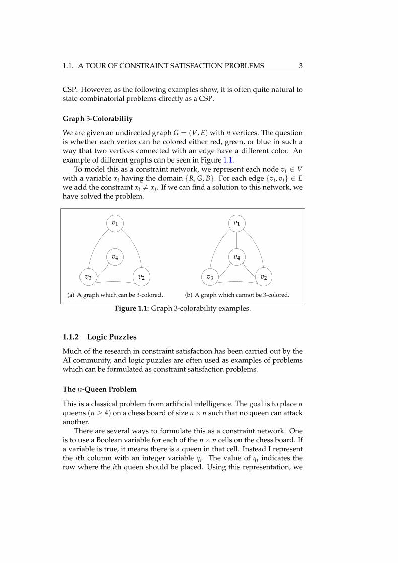
We are given an undirected graph G = (V, E) with n vertices. The questionis whether each vertex can be colored either red, green, or blue in such away that two vertices connected with an edge have a different color. Anexample of different graphs can be seen in Figure 1.1.
To model this as a constraint network, we represent each node vi ∈ Vwith a variable xi having the domain R, G, B. For each edge vi, vj ∈ Ewe add the constraint xi 6= xj. If we can find a solution to this network, wehave solved the problem.
v1
v4
v2v3
(a) A graph which can be 3-colored.
v1
v4
v2v3
(b) A graph which cannot be 3-colored.
Figure 1.1: Graph 3-colorability examples.
1.1.2 Logic Puzzles
Much of the research in constraint satisfaction has been carried out by theAI community, and logic puzzles are often used as examples of problemswhich can be formulated as constraint satisfaction problems.
The n-Queen Problem
This is a classical problem from artificial intelligence. The goal is to place nqueens (n ≥ 4) on a chess board of size n× n such that no queen can attackanother.
There are several ways to formulate this as a constraint network. Oneis to use a Boolean variable for each of the n× n cells on the chess board. Ifa variable is true, it means there is a queen in that cell. Instead I representthe ith column with an integer variable qi. The value of qi indicates therow where the ith queen should be placed. Using this representation, we

CHAPTER 1. INTRODUCTION 4
implicitly model the constraint (by creating n variables) that there shall beexactly one queen in each column.
The remaining constraints are:
|qi − qj| 6= i− j, for 1 ≤ i ≤ n, j > i and (1.1)
qi 6= qj, for 1 ≤ i ≤ n, j > i. (1.2)
Constraint (1.1) states that queen i and j cannot be on the same diagonaland Constraint (1.2) that queen i and j cannot be on the same row.
A solution to the n-queen problem is thus an assignment of values inthe range 1 to n to the variables q1, q2, . . . , qn such that the constraints in(1.1) and (1.2) are satisfied. For n = 8 there are 92 possible solutions to thisnetwork [Erbas et al., 1992]. One such solution is shown in Figure 1.2.
Figure 1.2: A solution to the 8-queen problem.
Who Owns the Zebra?
This problem is a classic example of a logic puzzle originally designed bythe English logician Charles L. Dodgson (aka. Lewis Carroll). There arefive houses, each of a different color and inhabited by people of differentnationalities, with different pets (one is a zebra), drinks (one drink is water),and cigarettes. We are given the following clues:
1. In each house there lives only one person.2. Each person has only one favorite drink, one pet, and smokes one
brand of cigarettes.3. The English person lives in the red house.4. The Spaniard owns the dog.5. Coffee is drunk in the green house.6. The Ukrainian drinks tea.

1.1. A TOUR OF CONSTRAINT SATISFACTION PROBLEMS 5
7. The green house is immediately to the right (your right) of the ivoryhouse.
8. The Old Gold smoker owns snails.9. Kools are smoked in the yellow house.
10. Milk is drunk in the middle house.11. The Norwegian lives in the first house on the left.12. The person who smokes Chesterfields lives next to the house with the
fox.13. The person who smokes Kools lives next to the house with the horse.14. The Lucky Strike smoker drinks orange juice.15. The Japanese smokes Parliaments.16. The Norwegian lives next to the blue house.
Questions: Who owns the zebra? Who drinks water?To model this as a constraint network, we can assign the houses num-
bers 1 to 5 and use 5 variables for house i, 1 ≤ i ≤ 5:
Ci ∈ red, green, ivory, yellow, blue, (1.3)Ni ∈ English, Spanish, Ukrainian, Norwegian, Japanese, (1.4)Pi ∈ zebra, dog, snails, fox, horse, (1.5)
Di ∈ water, coffee, tea, milk, juice, and (1.6)Si ∈ Old Gold, Kools, Chesterfield, Lucky Strike, Parliaments. (1.7)
We then have that Ci is the color of the ith house, Ni the nationality ofthe person living in the ith house and so on. Because all houses have adifferent color, all persons a different nationality, etc., we get the followingconstraints:
Ci 6= Cj, Ni 6= Nj, Pi 6= Pj, Di 6= Dj, Si 6= Sj 1 ≤ i ≤ 5, i < j (1.8)
The remaining clues can also be specified as constraints. Take for examplethe third clue, which can be expressed as:
Ni = English ⇐⇒ Ci = red 1 ≤ i ≤ 5. (1.9)
Constraint (1.9) states that if the nationality of the person living in the ithhouse is English then the ith house is red and vice versa. The remain-ing clues can be expressed in a similar way. The resulting network hasa single solution in which P5 = zebra, N5 = Japanese, D1 = water, andN1 = Norwegian. So the answer is “The Japanese owns the zebra” and“The Norwegian drinks water”.

CHAPTER 1. INTRODUCTION 6
1.2 Configuration
Configuration involves selecting combinations of predefined componentssubject to a number of problem constraints. The CSP paradigm offers an ad-equate framework for this task, and interactive configuration will be usedas the working example throughout this thesis.
Configuration problems may involve sales (sales configuration), design,manufacturing, installation, or maintenance. The components involvedneed not be physical but can also be paragraphs of a legal document, fi-nancial services, actions in a plan, etc.
The possibility to automate the product configuration task using a con-figuration system1 was recognized in the 1980’s, and is now a rapidly grow-ing industry. The following quote is from an article in Forbes Magazineabout a large vendor of configuration systems. It illustrates the complexityof some of the problems solved by configuration systems.
A [Boeing] 747 is made up of over 6 million parts, and acustomer can choose among hundreds of options. How manyseats? What kind of avionics? How many bathrooms? Do youwant carbon composite landing gear or steel? Every optionthe customer chooses affects the availability of other options,and changes the plane’s price. It takes the sales agent days orweeks working with company engineers to make sure all thechosen pieces fit together, re-negotiating the price at every step.[McHugh, 1996]
The preceding quote talks about the configuration of a large and com-plex product (a Boeing 747 airplane), probably sold to customers by a largeteam of salespersons and engineers. The ubiquitous use of the Internet hasenabled individual customers to buy products manufactured to their likingdirectly from an online store. But even in a relatively simple product suchas a Personal Computer (PC), there can be many dependencies among theavailable components. The picture in Figure 1.3 on the next page is froman online PC shop by one of the world’s largest PC manufacturers (whichshall remain anonymous). They appear not to be using a configuration sys-tem, but are instead relying on small textual notes on the screen advisingthe user about incompatible selections. The constraints that can be inferredfrom the notes are:
1. If you select more than three hard drives, you must select a hard drivebracket.
1Configuration systems are also known as product configuration systems (when usedto configure products) or sales configuration systems (when used in a sales process). I usethe more general term to emphasize that the usage is not restricted to the configuration ofproducts nor the usage in a sales process

1.2. CONFIGURATION 7
Figure 1.3: An example of an online store that could rely on a configurationsystem. Note how the incompatible selections are described using textualnotes.
2. If you select an Ultra 320 SCSI Controller Card, you must select atleast one Ultra 320 SCSI Hard Drive.
3. When ordering a RAID controller you must
(a) select only drives which have the same size and speed,(b) select a 1st drive that is RAID compatible, and(c) not select any IDE drives.
Considering that the screen shot only shows a subset of the availableoptions, it seems fairly easy to buy a product which will not function cor-rectly. For both a customer and a manufacturer, it is very expensive tohandle these types of configuration errors because manual intervention isrequired (call technical support, identify why the system does not work,perhaps return incorrect components, receive and install new necessarycomponents, etc.). If instead the manufacturer had used a configurationsystem, these constraints would have been taken into account automati-cally and an invalid combination of components could not be shipped tothe customer.

CHAPTER 1. INTRODUCTION 8
1.2.1 Elements of a Configuration System
At a high level, a constraint based configuration system is made up of twoparts, as shown in Figure 1.4:
1. A modeling part where a configuration model is created. The modelcan be created manually by a user2, automatically by extracting datafrom various enterprise systems or by a combination of the two ap-proaches.
2. A runtime part where the end users of the configuration system inter-act with the configuration model to determine the configuration thatsuit their needs (whether it is a product, a service, or something com-pletely different). The task of selecting the components is called theconfiguration task.
Components
Constraints
Modelcreation
RuntimeServices
Model
Internet
Figure 1.4: A high level view of a configuration system.
Creating a model involves specifying the components that are availableand the constraints between these components. There are many possibleways to capture this knowledge. Constraint networks provide a conve-nient way to describe the components available as well as the constraintsbetween them. In Section 4.4 on page 43, I will describe in more detail howa product model can be represented by a constraint network.
Changes to an already defined model involve changes in components(because some components are no longer available or new features be-come available to existing components) and/or changes to the constraints(because of new or changed components or because market requirementscause some combinations to be invalid). These changes occur infrequentlyrelative to the number of configuration tasks carried out. This observation
2This is only a conceptual view. For large models many users may be involved in creat-ing the model.
1.3. CONTRIBUTION 9
is important from an algorithmic point of view because it allows us to jus-tify spending some time to preprocess a model to speed up the algorithmsused during the configuration task.
The runtime part can come in many different incarnations dependingon the target users of the system. If used by a company’s customers, itmay be a web application running in a browser and accessed using theInternet. If used by a company’s salespersons, it may be an applicationrunning on the company’s intranet or on the salesperson’s laptop. If usedby field engineers, it may be an application running on a wireless devicesuch as a cellphone.
When the user has completed the configuration task, the resulting con-figuration is usually used in the next step of the business process. This mayinvolve printing a quote, creating an order or maybe assembling a docu-ment based on the user’s selections.
There are, of course, many other issues to an actual implementation of aconfiguration system (the actual process of capturing product knowledge,the language used for specifying this knowledge, how the model is dis-tributed to the salesperson’s laptop, what the model should look like whenpresented to the user, how the result of the configuration task should bestored, etc.). However, these issues are not essential to the contents of thisthesis.
1.3 Contribution
I have identified a number of requirements that must be fulfilled by an in-teractive constraint solver, in order to provide a good user interface. Drivenby these requirements I have identified three fundamental operations thatform the basis of an interactive constraint solver. They are:
Add-Constraint: Add a new constraint to an existing constraint network.
Remove-Constraint: Remove a previously added constraint from a con-straint network.
Restoration: Determine a set of constraints that restores satisfiability in aconstraint network when incompatible constraints have been added.
I have proposed algorithms for the fundamental operations, which runin worst-case polynomial time when the constraint network is restricted toan acyclic constraint network. By combining existing methods for constraintnetwork decomposition and solution synthesis, I have proposed a compi-lation scheme that compiles a general constraint network into an acyclicconstraint network required by the fundamental operations.

CHAPTER 1. INTRODUCTION 10
While the algorithms for the fundamental operations are polynomial,experiments show that the acyclic networks constructed by the compila-tion scheme are, in many cases, too large to handle if short response timesare required. To overcome this problem, I impose a further restrictionon the structure of the constraint network and propose a transformationmethod that transforms an acyclic constraint network into a uniform acyclicconstraint network. If a uniform acyclic network can be constructed, experi-ments show that the fundamental operations can be carried out in running-time suitable for interactive use.
All methods and algorithms presented in this thesis have been imple-mented and their performance evaluated on various constraint networks,many arising from real-life configuration problems. To my knowledge thisis the first experimental study where performance of interactive constraintsatisfaction methods have been evaluated on more than a single probleminstance.
1.4 Related Work
Methods for solving static constraint satisfaction problems have been ex-tensively studied. The book by Tsang [1993] covers many of the fundamen-tal concepts and algorithms.
As noted in the preceding sections, most of the algorithms developedwithin the classical CSP framework cannot be used to solve interactive de-cision support systems. The classical (static) CSP framework have beenextended with concepts that allow constraints to be added dynamically[Dechter and Dechter, 1988; Mittal and Falkenhainer, 1990]. The solutionmethods proposed, however, have not been directed towards interactiveuse.
The idea of compiling a constraint network into a form which allowsmore efficient processing is not new. Dechter and Pearl [1989] proposeda tree decomposition heuristic that transforms a constraint network into atree structure. Vempaty [1992] introduced the idea of using a finite-stateautomaton that represents the set of all solutions to a constraint network.Amilhastre et al. [2002] continued this idea and described how this automa-ton could be used to solve constraint satisfaction problems interactively.Møller [1995] proposed a method for synthesizing all solutions to a con-straint network and storing them compactly. Weigel and Faltings [1999]proposed a heuristic method, based on recursive spectral bisection, forcompiling a CSP into a minimal synthesis tree.
A Boolean Decision Diagram [Bryant, 1986] is a canonical representationof a Boolean function using a directed acyclic graph. BDDs are widely usedwithin the areas of circuit analysis and formal verification. A CSP can beviewed as a Boolean function that returns TRUE whenever a valid solution

1.5. OUTLINE OF THE THESIS 11
is passed as input. Bouquet and Jégou [1997] proposed a method that usedBDDs to solve dynamic constraint satisfaction systems.
Common for all these methods (as well as the methods proposed in thisthesis) is that an initial constraint network is transformed into a form thatallows efficient processing. Once the transformation is complete, efficientpolynomial time algorithms are used subsequently. Unfortunately, the pro-posed transformations are all exponential in time (and some in space). Thisis to be expected since, as we will see, the decision version of the constraintsatisfaction problem is NP-complete. The applicability of the differentmethods thus depends on how well they are able to transform the con-straint networks considered.
1.5 Outline of the Thesis
In Chapter 2 the definitions of general terms are given, the notation usedthroughout the thesis is fixed, and the basic definitions from graph the-ory and relational database theory are recalled. An experienced reader canskim this chapter.
Chapter 3 contains the formal definition of constraint networks, I provethat the decision version of a CSP is NP-complete, and survey solutionsmethods for the classical CSP. The chapter ends with a discussion of con-ditions in which a CSP becomes tractable.
In Chapter 4, I identify a list of usability requirements for an interactiveconstraint satisfaction system and proceed with an extension of the clas-sical CSP framework, which can be used to describe interactive constraintsatisfaction problems. From these requirements and definitions, I identifyoperations that are fundamental for an interactive constraint satisfactionsystem and describe them formally. Polynomial-time algorithms, whichoperate on an acyclic constraint network, are then presented for the funda-mental operations.
In Chapter 5, I describe an existing method for synthesizing solutionsand an existing method for decomposing constraint networks, and showhow they can be combined to transform any constraint network into anacyclic constraint network
Chapter 6 highlights the important parts of an implementation of thealgorithms described in chapters 4 and 5. This chapter also contains theexperimental results that have been obtained by running the implementedalgorithms on several different constraint networks. The constraint net-works used in the experiments consist of real life problems that have beenencountered in various customer projects, problems mentioned in other re-search articles and logic puzzles.
In Chapter 7, I propose to further restrict the structure of an acyclicconstraint network to obtain a uniform acyclic constraint network to improve

CHAPTER 1. INTRODUCTION 12
the response time of the fundamental operations. A tree transformationmethod is proposed which transforms an acyclic network into a uniformacyclic network. The chapter is concluded by an experimental evaluationof the proposed methods.
Chapter 8 concludes the thesis by highlighting the results and by propos-ing some further areas of research.
CHAPTER 2
Preliminaries
In this chapter the definitions of general terms are given, the notation usedthroughout the thesis is fixed and the basic definitions from graph theoryand relational database theory are recalled. An experienced reader canskim this chapter.
2.1 Graph Theory
Definition 2.1. A graph G = (V, E) is a structure where V is a finite set ofvertices or nodes and E a finite set of edges or arcs1. For an undirected grapheach edge is an unordered pair of vertices, and for a directed graph each edgeis an ordered pair of vertices.
Definition 2.2. A graph G′ = (V ′, E′) is a subgraph of G = (V, E) if V ′ ⊆ Vand E′ ⊆ E.
Definition 2.3. A clique in an undirected graph G = (V, E) is a subset V ′ ⊆V of vertices, each pair which is connected by an edge in E. A clique is amaximal clique if it is not a proper subset of any other clique.
Definition 2.4. A hypergraph H = (V, S) is a structure where V is a finiteset of vertices and S a finite set of hyperedges. Each hyperedge E is a subsetof the vertices, i.e. E ⊆ V. A hypergraph is reduced if, and only if, nohyperedge is a proper subset of another.
1I will frequently use the terms “node” and “arc” instead of “vertex” and “edge” re-spectively, to keep with the tradition in the AI community. This emphasizes the connectionbetween the graph representation of constraint networks and some of the fundamental al-gorithms such as Node Consistency and Arc Consistency.
13

CHAPTER 2. PRELIMINARIES 14
Definition 2.5. For a hypergraph H = (V, S), the primal graph of H is anundirected multi-graph (V, E) where every two vertices joined by a hyper-edge in S is joined by an edge in E.
2.2 Relational Database Theory
As we will see in the following chapter, there is a close relationship betweenconstraint networks and the relational data model used in database systemsas initially defined by Codd in his seminal article [Codd, 1970]. Both userelations as the primary notation for representing data or knowledge. Adatabase is a finite set of relations.
Definition 2.6. A relation consists of a scheme and an instance:
1. A scheme is a finite set of attributes. Each attribute is associated witha set of values, called its domain.
2. A tuple over a scheme is a mapping, that associates with each attributeof the scheme a value from its corresponding domain.
3. An instance over a scheme is a finite set of tuples over that scheme.
Since relations are sets, the general set operations apply to relationswith the restriction that both relations must have the same scheme. Giventwo relations R and S with the same scheme, the intersection of R and S,denoted R∩ S, is the relation containing tuples that are in both R and S; theunion R ∪ S is the relation containing the tuples that are in either R or S orboth, and the difference R− S is the relation containing the tuples that arein R but not in S.
Many additional operations have been defined on relations. These op-erations are part of the relational algebra [Codd, 1970]. Of these, we willmake use of projection and join which will be defined next.
Definition 2.7. Let R be a relation with scheme Y and Z ⊆ Y a set of at-tributes. Let r be an instance over Y. The projection of r onto Z, denotedπZ(r), is a relation with scheme Z and instance t|Z | t ∈ r where t|Z de-notes the tuple formed from t by keeping only those components associatedwith the attributes in Z.
Definition 2.8. Let R be a relation with scheme Y and instance r. Let S be arelation with scheme Z and instance s. The join2 of R and S, denoted R 1 S,
2The operation defined here is sometimes referred to as natural join to distinguish fromthe more general theta join. Here we use the short form since it does not give rise to confu-sion.

2.3. MODEL OF COMPUTATION 15
is defined to be the relation with scheme Y ∪ Z and an instance containingthe following set of tuples:
t | t is a tuple over Y ∪ Z , t|Y ∈ r, t|Z ∈ s.
Again, t|Z denotes the tuple t restricted to Z.
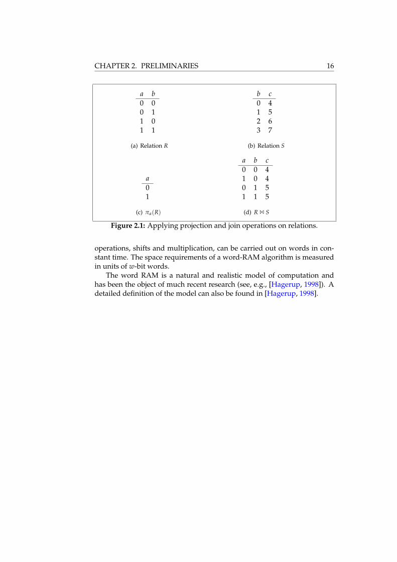
The projection operator is used to remove certain components of thetuples in a relation, and the join operator is used to combine two relationson all their common variables. If there are no common variables, the joinoperator behaves as a Cartesian product. Since the results of the operatorsare again relations, the operators can be combined.
2.2.1 Representing Relations
In Definition 2.6 on the facing page, schemes and tuples are formally de-fined in terms of sets. This allows specifying tuples without fixing the at-tribute order. Consider a relation with scheme a, b, c and the domainof each attribute being the set of integers. A tuple over this scheme isb 7→ 2, c 7→ 3, a 7→ 1, where b 7→ 2 is used to denote that the attribute bmaps to the value 2.
For notational convenience, however, I will express tuples as orderedsequences, with an implied ordering for the attributes of each relation.Thus with the attribute ordering (a, b, c) the same tuple is expressed as(1, 2, 3). A relation is usually depicted using a table with the first row rep-resenting the attributes, a horizontal line and a row for each tuple in theinstance:
a b c1 2 3
Similarly, the relation instance is expressed as an ordered sequence oftuples and R[i] denotes the ith tuple of relation instance R. The number oftuples in a relation instance is denoted by |R|.
Example 2.1. The result of applying the projection and join operators totwo relations R and S is shown in Figure 2.1 on the next page.
2.3 Model of Computation
The model of computation used is the unit-cost word RAM. For a positiveinteger parameter w, called the word length, the memory cells of a wordRAM store w-bit words, viewed as integers in 0, . . . , 2w−1 or as bit vec-tors in 0, 1w. Standard operations, including addition, bitwise Boolean
CHAPTER 2. PRELIMINARIES 16
a b0 00 11 01 1
(a) Relation R
b c0 41 52 63 7
(b) Relation S
a01
(c) πa(R)
a b c0 0 41 0 40 1 51 1 5
(d) R 1 S
Figure 2.1: Applying projection and join operations on relations.
operations, shifts and multiplication, can be carried out on words in con-stant time. The space requirements of a word-RAM algorithm is measuredin units of w-bit words.
The word RAM is a natural and realistic model of computation andhas been the object of much recent research (see, e.g., [Hagerup, 1998]). Adetailed definition of the model can also be found in [Hagerup, 1998].

CHAPTER 3
Constraint Satisfaction Problems
In the present chapter, the terminology, concepts and definitions relatingto constraint satisfaction problems are introduced and some of the funda-mental algorithms for solving them are surveyed.
Due to the diversity of research, much of the terminology related toconstraint satisfaction is unfortunately ambiguous. I have chosen the def-initions to ease the presentation of the subsequent material while keepingin agreement with most of the existing literature.
3.1 Constraint Networks
An instance of a constraint satisfaction problem can be described by a con-straint network1.
Definition 3.1 (Constraint Network). A constraint network is a triple R =(X, D, C) where
1. X is a finite set of variables.
2. D is a function that maps each variable x in X to a finite set of values,written D(x), which it is allowed to take. The set D(x), called thedomain of x, is also denoted Dx.
3. C is a finite set of constraints. Let S = xk, . . . , x` ⊆ X. Each con-straint CS ∈ C is a relation with scheme S and instance CS. The set
1The term “network” is used to reflect the historical perspective when focus was re-stricted to constraints whose dependencies can naturally be captured by simple graphs aswell as to emphasize the importance of the constraint dependency structure to the solutionalgorithms.
17

CHAPTER 3. CONSTRAINT SATISFACTION PROBLEMS 18
S is the scope of the constraint, and |S| denotes the arity of the con-straint. Each tuple in the instance CS ⊆ Dxk × · · · × Dx`
specifies acombination of values which the constraint allows.
In general, domains can be infinite which in turn implies that the constraintrelations can be infinite, but we only consider the case where variables havefinite domains (sometimes called finite domain constraint satisfaction prob-lems). The constraint representation chosen in Definition 3.1 on the preced-ing page is extensional, i.e., an explicit enumeration of the tuples that areallowed by the constraint. Other representations are possible, e.g., an in-tensional representation where a constraint is represented in symbolic formsuch as predicate logic.
Without loss of generality I assume that all constraints have a uniquescope, i.e., for all CS, CR ∈ C, CS 6= CR we have S 6= R. To simplify the nota-tion, I usually denote the constraint Cx,y,z as Cx,y,z or even Cxyz, when noconfusion can arise from this simplified notation. A constraint with arityone is called a unary or domain constraint (since it restricts the possible val-ues of a variable). A constraint with arity two is called binary. A networkwith only binary constraints is called a binary constraint network, otherwiseit is called a general constraint network.
Definition 3.2. Let R = (X, D, C) be a constraint network. An assignmentof the value a ∈ Dx to the variable x ∈ X is denoted 〈x, a〉. An instantiationof a set of variables xk, . . . , x` ⊆ X is a simultaneous assignment of valuesto the variables xk, . . . , x` and is denoted 〈xk, ak〉, . . . , 〈x`, a`〉.
For simplicity, we often perceive an instantiation as a tuple (ak, . . . , a`) overthe scope xk, . . . , x` and denote the instantiation briefly as axk ,...,x` orsimply a if the scope is well defined or unimportant.
Definition 3.3. An instantiation a satisfies a constraint CS if a|S ∈ CS. LetR = (X, D, C) be a constraint network. An instantiation aT, where T ⊆ X,is consistent relative to R if, and only if, aT satisfies all constraints CS ∈ Csuch that S ⊆ T.
Definition 3.4. A solution of the constraint network R = (X, D, C) is aninstantiation of all variables in X which is consistent relative to R. The setof all solutions to a constraint network R is denoted Sol(R).
A network R is called satisfiable if Sol(R) 6= ∅ and unsatisfiable if Sol(R) =∅. Two networks defined on the same set of variables are considered equiv-alent if they have the same set of solutions. A constraint is redundant ifremoval of the constraint does not change the set of all solutions. For aconstraint network R = (X, D, C), any subset of variables I ⊆ X induces asubnetwork ofRwhich has variables I, domains D and the set of constraintsis a subset of C:
CS | CS ∈ C, S ∩ I 6= ∅. (3.1)

3.1. CONSTRAINT NETWORKS 19
Given a constraint networkR, a CSP can be classified into the followingcategories:
1. Determine whether the network R is satisfiable.
2. Find a solution to the networkR, with no preference as to which one.
3. Find the set of all solutions Sol(R).
4. Find an optimal solution to the network R, where optimality is de-fined by a function on the variables in R.
Optimal or approximatively optimal solutions are often required in plan-ning and scheduling problems where the objective is to, e.g., minimize thetime required to finish a schedule.
3.1.1 Constraint Network Properties
A constraint network can be characterized by various parameters.
n: the number of variables, |X|,
d: the size of the largest domain, maxx∈X|Dx|,
e: the number of constraints, |C|,
r: the size of the largest scope, maxCS∈C|S|, and,
t: the largest number of tuples in any constraint relation, maxCS∈C|CS|.
Definition 3.5. The tightness of a constraint CS is the ratio between the num-ber of tuples in the constraint relation and the number of possible instanti-ations of the variables in S
|CS|∏x∈S|Dx|
. (3.2)
The universal constraint over the variables S, denoted US, allows every in-stantiation of the variables in the scope S. It is the most relaxed constraintpossible and has tightness 1.
In general, the number of tuples in a constraint with scope S is boundedby ∏x∈S|Dx|, which is the number of tuples in the universal constraint withscope S. Frequently, constraints are quite tight. For binary constraints wehave, e.g., the universal constraint with t ≤ d2, but functional constraintshave t ≤ d.

CHAPTER 3. CONSTRAINT SATISFACTION PROBLEMS 20
Definition 3.6. The tightness of a constraint network R = (X, D, C) is mea-sured by the number of solutions over the number of possible instantiationsfor all variables
|Sol(R)|∏x∈X|Dx|
. (3.3)
Definition 3.7. The size of a CSP described by a constraint network R =(X, D, C) is defined as
∑CS∈C
|S||CS| = O(ert). (3.4)
Example 3.1. Let us construct a simple constraint network to illustrate thedefinitions. As an example we use the 4-queen problem introduced in Sec-tion 1.1.2 on page 3. As noted we have 4 integer variables, one for eachqueen. So we have X = q1, q2, q3, q4 and Dx = 1, 2, 3, 4 for each x ∈ X.The two constraints in Equation (1.1) and Equation (1.2) can be combinedso we get a total of six binary constraints. The constraints are shown in thefollowing where the notation C12 is used to denote Cq1,q2:
C12 = (1, 3), (1, 4), (2, 4), (3, 1), (4, 1), (4, 2)C13 = (1, 2), (1, 4), (2, 1), (2, 3), (3, 2), (3, 4), (4, 1), (4, 3)C14 = (1, 2), (1, 3), (2, 1), (2, 3), (2, 4), (3, 1), (3, 2), (3, 4), (4, 2), (4, 3)C23 = (1, 3), (1, 4), (2, 4), (3, 1), (4, 1), (4, 2)C24 = (1, 2), (1, 4), (2, 1), (2, 3), (3, 2), (3, 4), (4, 1), (4, 3)C34 = (1, 3), (1, 4), (2, 4), (3, 1), (4, 1), (4, 2).
There are only two solutions to the 4-queen problem as shown in Fig-ure 3.1(a) and Figure 3.1(b). Figure 3.1(c) on the facing page shows a con-sistent instantiation that cannot be extended to a full solution.
3.1.2 Links with Relational Database Theory
As noted in [Gyssens et al., 1994] the definitions given so far have closeconnections to relational database theory. For any constraint network R =(X, D, C), the following connections can be established:
• The variables in X can be interpreted as attributes.
• The domain associated with an attribute is the domain of the corre-sponding variable in X.

3.1. CONSTRAINT NETWORKS 21
(a) Solution corre-sponding to 3, 1, 4, 2.
(b) Solution corre-sponding to 2, 4, 1, 3.
(c) Consistent instantia-tion not part of a solu-tion.
Figure 3.1: Some consistent instantiations of the 4-queen problem. Not allconsistent instantiations can be extended to a full solution.
• The valid combinations of values with scope S ⊆ X is a tuple over thescheme with the set of attributes S.
This gives rise to two alternative views of a constraint networkR = (X, D, C).
1. The set of all solutions can be represented by the database consistingof a single relation with scheme X and instance Sol(R).
2. The constraint network can be represented by the database RCS |CS ∈ C where RCS is a relation with scheme S and instance CS.
It follows from these definitions that for a constraint networkR = (X, D, C),Sol(R) is equal to the relation 1CS∈C CS (the join of all relations in C). Ta-ble 3.1 summarizes the terminology.
Constraint Terminology Database Terminologyconstraint network ≡ database
variable ≡ attributedomain ≡ attribute domain
constraint ≡ relationconstraint scope ≡ scheme
constraint relation ≡ instanceset of solutions ≡ join of all tables
Table 3.1: Constraint and database terminology. Adapted from [Pearsonand Jeavons, 1997].
3.1.3 Structure of Constraint Networks
The structure, or topology, of a constraint network can be described usingvarious objects as the following definitions show.
CHAPTER 3. CONSTRAINT SATISFACTION PROBLEMS 22
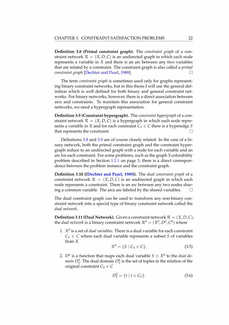
Definition 3.8 (Primal constraint graph). The constraint graph of a con-straint network R = (X, D, C) is an undirected graph in which each noderepresents a variable in X and there is an arc between any two variablesthat are related by a constraint. The constraint graph is also called a primalconstraint graph [Dechter and Pearl, 1989].
The term constraint graph is sometimes used only for graphs represent-ing binary constraint networks, but in this thesis I will use the general def-inition which is well defined for both binary and general constraint net-works. For binary networks, however, there is a direct association betweenarcs and constraints. To maintain this association for general constraintnetworks, we need a hypergraph representation.
Definition 3.9 (Constraint hypergraph). The constraint hypergraph of a con-straint network R = (X, D, C) is a hypergraph in which each node repre-sents a variable in X and for each constraint CS ∈ C there is a hyperedge Sthat represents the constraint.
Definitions 3.8 and 3.9 are of course closely related: In the case of a bi-nary network, both the primal constraint graph and the constraint hyper-graph reduce to an undirected graph with a node for each variable and anarc for each constraint. For some problems, such as the graph 3-colorabilityproblem described in Section 1.1.1 on page 3, there is a direct correspon-dence between the problem instance and the constraint graph.
Definition 3.10 ([Dechter and Pearl, 1989]). The dual constraint graph of aconstraint network R = (X, D, C) is an undirected graph in which eachnode represents a constraint. There is an arc between any two nodes shar-ing a common variable. The arcs are labeled by the shared variables.
The dual constraint graph can be used to transform any non-binary con-straint network into a special type of binary constraint network called thedual network.
Definition 3.11 (Dual Network). Given a constraint networkR = (X, D, C),the dual network is a binary constraint network Rd = (Xd, Dd, Cd) where
1. Xd is a set of dual variables. There is a dual variable for each constraintCS ∈ C where each dual variable represents a subset S of variablesfrom X
Xd = S | CS ∈ C. (3.5)
2. Dd is a function that maps each dual variable S ∈ Xd to the dual do-main Dd
S. The dual domain DdS is the set of tuples in the relation of the
original constraint CS ∈ C
DdS = t | t ∈ CS. (3.6)

3.1. CONSTRAINT NETWORKS 23
3. Any two dual variables sharing an original variable must obey the re-striction that their shared original variables must have the same val-ues. The constraints in Cd are thus
Cd = CdS,T | S, T ∈ Xd, S ∩ T 6= ∅ (3.7)
where CdS,T is the binary constraint
CdS,T = (u, v) | u ∈ CS, v ∈ CT, u|S∩T = v|S∩T. (3.8)
Thus all the constraints in the dual network are in some sense equality con-straints. It should be clear that if we found a solution to the dual networkwe would also, by mapping the solution back to the original variables, finda solution to the original problem. In this way all general constraint net-works can be transformed into binary networks and solved using binarynetwork techniques. This is useful, since many CSP algorithms are definedonly for binary networks. Other encodings exist for transforming a generalnetwork to a binary network. Bacchus et al. [2002] compare some of theencodings when used in conjunction with search algorithms.
Example 3.2. Consider the following constraint network with five variablesand three constraints:
X = model, case, ide, scsi, cpuDmodel = home, office
Dcase = desktop, towerDide = none, 40gb, 80gbDscsi = none, 18gb, 36gbDcpu = PIII, PIV, AMD
C = Cmodel,cpu,case, Cide,scsi, Ccase,scsi
model cpu casehome PIII desktophome AMD desktopoffice PIII desktopoffice PIII toweroffice PIV desktopoffice PIV toweroffice AMD desktopoffice AMD tower
ide scsinone 18gbnone 36gb40gb none80gb none
case scsidesktop nonetower nonetower 18gbtower 36gb
The different graph representations for this constraint network are shownin Figure 3.2 on page 25. The dual network is a constraint network with

CHAPTER 3. CONSTRAINT SATISFACTION PROBLEMS 24
three variables: one for each constraint in the original problem, and twobinary constraints: one for each edge in the dual constraint graph. Thedomains of the dual variables are the tuples of the corresponding originalconstraints. Note that if we depicted the primal graph of the dual problem,the topology would be equivalent to the dual graph of the original problem.
Xd = model, cpu, case, ide, scsi, case, scsiDdmodel,cpu,case = Cmodel,cpu,case
Ddide,scsi = Cide,scsi
Ddcase,scsi = Ccase,scsi
Cd = Cd(model,cpu,case,case,scsi), Cd
(case,scsi,case,ide)
model, cpu, case case, scsi(home, PIII, desktop) (desktop, none)
(home, AMD, desktop) (desktop, none)(office, PIII, desktop) (desktop, none)(office, PIV, desktop) (desktop, none)
(office, AMD, desktop) (desktop, none)(office, PIII, tower) (tower, none)(office, PIV, tower) (tower, none)
(office, AMD, tower) (tower, none)(office, PIII, tower) (tower, 18gb)(office, PIV, tower) (tower, 18gb)
(office, AMD, tower) (tower, 18gb)(office, PIII, tower) (tower, 36gb)(office, PIV, tower) (tower, 36gb)
(office, AMD, tower) (tower, 36gb)
case, scsi ide, scsi(desktop, none) (40gb, none)(desktop, none) (80gb, none)(tower, none) (40gb, none)(tower, none) (80gb, none)(tower, 18gb) (none, 18gb)(tower, 36gb) (none, 36gb)
3.2 Complexity of Constraint Satisfaction
Given a CSP, we can derive a corresponding decision problem:
Definition 3.12 (CONSTRAINT SATISFIABILITY). The decision version of aconstraint satisfaction problem has a triple (X, D, C) as an input, where X,

3.2. COMPLEXITY OF CONSTRAINT SATISFACTION 25
scsiide
model cpu case
(a) Constraint hypergraph
scsiide
model cpu case
(b) Primal constraint graph
Cmodel,cpu,case
Cide,scsi
Ccase,scsi
case
scsi
(c) Dual constraint graph
Figure 3.2: Different graph representations of the constraint network inExample 3.2.
D and C are as in Definition 3.1, and yields “yes” or “no” as an output. Theoutput is “yes” if the constraint network (X, D, C) has a solution and “no”otherwise. This decision problem is called the CONSTRAINT SATISFIABIL-ITY (CS) problem.
Clearly, finding any solution to a constraint network, can be used tosolve the corresponding decision problem, i.e., finding a solution, all solu-tions or an optimal solution is as difficult as CS. In the following, we willprove that CS is NP-complete. First we need to introduce a well-knownNP-complete decision problem (see, e.g., Cormen et al. [2001] for moredetails):
Definition 3.13 (3-CNF-SAT). An input of 3-CNF-SAT is a Boolean formulacomposed of
1. Boolean variables: x1, x2, . . . ;
2. Boolean connectives such as ∧ (AND), ∨ (OR), ¬ (NOT); and
3. parentheses.
A literal in a Boolean formula is an occurrence of a variable or its negation.A Boolean formula is in conjunctive normal form, or CNF, if it is expressed
CHAPTER 3. CONSTRAINT SATISFACTION PROBLEMS 26
as a logical AND of clauses, each of which is the logical OR of one or moreliterals. A Boolean formula is in 3-conjunctive normal form, or 3-CNF, if eachclause has exactly three distinct literals.
In 3-CNF-SAT, we are asked whether a given Boolean formula in 3-CNFhas a satisfying assignment, i.e., a set of values for the variables that causesthe formula to evaluate to true.
Lemma 3.1. 3-CNF-SAT is polynomial-time reducible to CS.
Proof. Let θ = C1∧C2∧ · · ·Ck be a Boolean formula in 3-CNF with k clauses.From θ we need to create the input (X, D, C) to the decision problem CS,where X is the variables, D the variable domains and C the constraints. Itis created as follows.
1. For each distinct variable xi in θ, we add xi to X.
2. For each variable xi in X, we let Dxi = 0, 1.
3. For each clause Cr = (l1 ∨ l2 ∨ l3) in θ, we create a constraint CS. Thescope S contains the (not necessarily distinct) variables appearing inthe literals l1, l2 and l3. The constraint relation CS contains a 3-tuplefor each satisfying assignment to Cr.
This reduction is linear in the number of clauses in θ since there are at most3k variables, k constraints, and each constraint relation has at most 23 = 8tuples. It is clear that θ is satisfiable if, and only if, the constraint network(X, D, C) has a solution.
Theorem 3.2. CS is NP-complete.
Proof. LetR = (X, D, C) be the input of a CSP decision problem where X isthe set of variables, D their domains and C the set of constraints. First wenote that CS is in NP : Given an instantiation a of all variables in X, verifya|S ∈ CS for each CS ∈ C. The verification can be done in time polynomialin the size ofR. By NP-completeness of 3-CNF-SAT and Lemma 3.1, CS isNP-complete.
3.3 CSP Solution Methods
A CSP can be solved using the generate-and-test method (also know as “theBritish Museum Algorithm” according to Hoare [1989]), where each possi-ble instantiation of the variables is systematically generated and then testedto see if it satisfies all the constraints. The first such instantiation found is asolution. The number of instantiations generated in the worst case (whichoccurs when the network is unsatisfiable) is O(dn), i.e., exponential in thenumber of variables. Figure 3.3(a) on page 28 shows the search tree whena generate-and-test algorithm is applied to an unsatisfiable problem.

3.3. CSP SOLUTION METHODS 27
By using backtracking [Bitner and Reingold, 1975], a potentially moreefficient method can be constructed. During search, variables are instanti-ated according to some ordering called the instantiation order, and when allvariables in a constraint have been instantiated, the constraint is checked.Whenever a partial instantiation violates a constraint, backtracking is per-formed to the most recently instantiated variable with uninstantiated val-ues left in the domain, thereby eliminating a subspace from the Cartesianproduct of the variable domains. A naive backtracking algorithm (usuallycalled chronological backtracking) is shown in Algorithm 3.1.
BACKTRACK(a, X, D, C)1 . a is the current instantiation2 if X = ∅3 return a4 else5 x ← some variable from X6 repeat7 v ← some value from Dx8 Dx ← Dx − v9 if a ∪ 〈x, v〉 is consistent
10 r ←BACKTRACK(a ∪ 〈x, v〉, X − x, D, C)11 if r 6= NIL
12 return r13 until Dx = ∅14 return NIL
Algorithm 3.1: A simple backtracking solver.
Given a network R = (X, D, C) the call BACKTRACK(∅, X, D, C) re-turns a solution if the network is satisfiable, otherwise NIL is returned.While BACKTRACK still generates O(dn) instantiations in the worst case,the ability to eliminate subspaces of the search tree makes it more efficientin most cases. Figure 3.3(b) on the next page shows the search tree whenBACKTRACK is applied to an unsatisfiable problem. The left subtree illus-trates the search space which is eliminated because the first variable assign-ment is inconsistent. It should be clear from this figure that the ordering inwhich variables are instantiated is important. In this example, if the firstassignment was instead last, all instantiations would have to be tested, i.e.BACKTRACK deteriorates to generate-and-test.
There are two drawbacks in the standard backtracking scheme pre-sented here. One is trashing [Gaschnig, 1979] where search fails repeatedlyfor the same reason. If, for example, the constraint Cxi ,xk specifies that aparticular assignment to xi disallows all potential values for xk then BACK-TRACK fails when instantiating xk for all values in Dxk , repeating this fail-ure for all instantiations of variables xj for i < j < k. The other drawback

CHAPTER 3. CONSTRAINT SATISFACTION PROBLEMS 28
cc
cc BBBc
J
JJcc BBBc
ZZ
ZZ cc
c BBBc
JJJcc BBBc
(a) Generate-and-test
c
AA
AA
AA
Z
ZZZ c
cc BBBc
J
JJcc BBBc
(b) Backtracking
Figure 3.3: Search tree example for an unsatisfiable network. Each edgerepresents an assignment of a value to a variable, each level in the treecorresponds to a variable. In (a) all combinations are tested before unsatis-fiability is detected. In (b) all combinations in the left branch are skippedsince the first assignment to the first variable is found to be inconsistent.
is having to perform redundant work. If, for example during a constraintcheck, an instantiation of a subset of variables is found to be consistent andthen deeper in the search tree, the instantiation has not changed; then thereis no need to check these variables again.
Many variations on the naive backtracking scheme have been proposedto cope with these drawbacks as well as finding a good instantiation order.While theses methods differ in the number of constraint checks they mustperform, they are all exponential in the worst case. For all but the small-est problems this makes them unsuitable for use in an interactive setting. Iwill therefore not go into more detail about search techniques, but refer in-terested readers to the papers by Miguel and Shen [2001a,b] which containa survey on many of the known search strategies. Kondrak and van Beek[1997] present a theoretical evaluation of several backtracking algorithms.
3.3.1 Consistency in Binary Networks
Preprocessing a constraint network creates an equivalent network that iseasier to solve, usually using some search algorithm. Algorithms that per-form preprocessing are often called consistency enforcing, inference or con-straint propagation algorithms.
The simplification involves removing domain values that can never bepart of a solution, simplifying constraints by removing tuples that can neverbe part of a solution or introducing new tighter constraints that can beinferred by propagating information from existing constraints. The mostwidely used levels of consistency in binary networks are called node, arcand path consistency, and were defined by Mackworth [1977b].

3.3. CSP SOLUTION METHODS 29
Node Consistency
Definition 3.14. A variable is node consistent if all values in the domainsatisfy the unary constraint on that variable2. A constraint network is nodeconsistent if all variables are node consistent.
Achieving node consistency amounts to checking all domain values to seeif they satisfy the unary constraint on the corresponding variable. We canuse relational algebra to specify node consistency, in which case we get
Dx ← Dx ∩ Cx, for all x ∈ X, Cx ∈ C, (3.9)
where we have used the fact that the domain of a variable x can be viewedas a relation with scope x and instance Dx.
An algorithm for making a network node consistent is shown in Algo-rithm 3.2. The time complexity of NC is O(dn) if we assume the constraintcheck a /∈ Cx takes constant time.
NC(X, D, C)1 for each x ∈ X2 for each a ∈ Dx3 if a /∈ Cx4 Dx ← Dx − a
Algorithm 3.2: Make network (X, D, C) node consistent.
Arc Consistency
Definition 3.15. LetR = (X, D, C) be a node consistent constraint networkwith Cxy ∈ C. A variable x is arc consistent relative to y if, and only if, forevery value a ∈ Dx there exists a value b ∈ Dy such that (a, b) ∈ Cxy. Anarc x, y in the constraint graph of R is arc consistent if and only if x isarc consistent relative to y and y is arc consistent relative to x. A constraintnetwork is arc consistent if, and only if, all arcs are arc consistent.
Consider an instantiation 〈x, a〉 of some variable x. If there is a constraintCxy and there is no value b ∈ Dy such that (a, b) ∈ Cxy, then we can removethe value a from Dx without affecting any solution.
Arc consistency algorithms have received a great deal of attention inthe CSP literature. As a result, a number of algorithms for achieving arcconsistency have been proposed. They have traditionally been named AC-n where n increases with each improvement or specialization of previousalgorithms.
2Recall that we assumed that all constraint scopes are unique. This implies that therecan be at most one unary constraint on any given variable.

CHAPTER 3. CONSTRAINT SATISFACTION PROBLEMS 30
Algorithm REVISE shown in Algorithm 3.3, makes a variable x arc con-sistent relative to a variable y, by removing values from the domain of xthat cannot be part of a solution when considering the constraint Cxy. Wecan again use relational algebra to describe the result of REVISE:
Dx ← Dx ∩ πx(Cxy 1 Dy). (3.10)
Algorithm REVISE can be used to create an algorithm for achieving arcconsistency. A naive brute force arc consistency algorithm called AC-1 (firstproposed by Mackworth [1977b]) is shown in Algorithm 3.4.
REVISE(x, y, X, D, C)1 for each a ∈ Dx2 for each b ∈ Dy3 if (a, b) /∈ Cxy4 Dx ← Dx − a
Algorithm 3.3: Make x arc consistent relative to y.
AC-1(X, D, C)1 repeat2 for each Cxy ∈ C3 REVISE(x, y, X, D, C)4 REVISE(y, x, X, D, C)5 until no domain is changed
Algorithm 3.4: A naive algorithm for achieving arc consistency.
The time complexity of REVISE is O(d2) if we assume the constraintcheck (a, b) /∈ Cxy takes constant time. The calls to REVISE in lines 2–4 thustake time O(ed2) and may in the worst case delete only one domain value.There areO(nd) domain values, so the worst-case time complexity of AC-1is O(ned3).
Several improvements to the naive AC-1 algorithm have been proposed.When a value is removed from a domain, AC-1 checks all constraints again.AC-3 [Mackworth, 1977b] improves the running time to O(ed3) by consid-ering only the constraints which could be affected by a removal of values.A lower bound for achieving arc consistency is Ω(ed2) since this is the timerequired to check arc consistency for all constraints. Mohr and Henderson[1986] describe an optimal algorithm AC-4 based on the notion of support; adomain value is supported if there exists a compatible value in the domainof every adjacent variable. When a value a is removed from the domainof x, it is not always necessary to examine all binary constraints Cxy. Wecan ignore those values in Dy which do not rely on a for support. Thespace complexity of AC-4 is O(ed2). This is improved to O(ed) in AC-6 byBessière [1994].

3.3. CSP SOLUTION METHODS 31
Path Consistency
Definition 3.16. Let R = (X, D, C) be a node consistent constraint net-work. A path (x0, . . . , xm) of length m in the constraint graph for R is pathconsistent if and only if for any consistent instantiation (v0, vm) ∈ Cx0,xm
there is a sequence of values of vj ∈ Dj, 1 ≤ j < m such that (v0, v1) ∈Cx0,x1 , . . . , (vm−1, vm) ∈ Cxm−1,xm . A constraint network is path consistent if,and only if, every path in its constraint graph is path consistent.
The following theorem provides a method for achieving path consis-tency.
Theorem 3.3 ([Montanari, 1974]). A constraint network is path consistent if,and only if, every path of length 2 of a complete constraint graph is path consistent.
Achieving path consistency thus involves tightening of constraints or, ifno constraints exists between two variables, introducing new binary con-straints. In analog to REVISE, which deals with two variables for achievingarc consistency, we define REVISE-3 shown in Algorithm 3.5 that takes apath (i, j, k) of length 2 and makes it path consistent by modifying the con-straint Cik (which may be the universal constraint if the original networkdoes not contain a constraint between i and k) by deleting tuples that can-not be extended consistently by including values from j.
REVISE-3(i, j, k, X, D, C)1 for each (vi, vk) ∈ Cik2 for each vj ∈ Dj3 if (vi, vj) /∈ Cij or (vj, vk) /∈ Cjk4 Cik ← Cik − (vi, vk)
Algorithm 3.5: Make (i, j, k) path consistent. Removes tuples from con-straint Cik which cannot be extended consistently to values of j.
We can again use relational algebra to describe the result of REVISE-3:
Cik ← Cik ∩ πik(Cij 1 Dj 1 Cjk). (3.11)
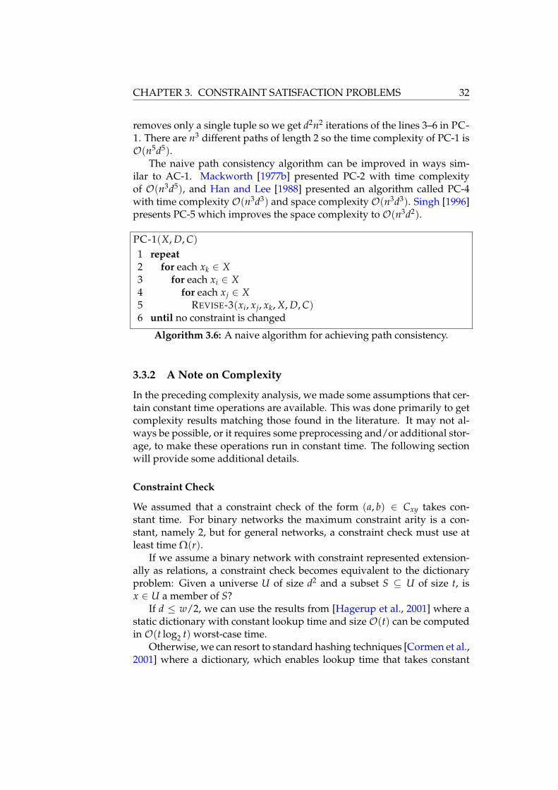
From Theorem 3.3 it follows that path consistency can be achieved by call-ing REVISE-3 with all possible paths of length 2. Such a naive path consis-tency algorithm called PC-1 is shown in Algorithm 3.6 on the next page.Note that achieving path consistency, in general, changes the structure ofthe constraint graph of a network by introducing new constraints.
The time complexity of REVISE-3 is O(d3) since there are at most d2 tu-ples in each constraint and at most d values in each domain. We assumethat both a constraint check and a set modification takes constant time.There are n variables so there can be at most n2 binary constraints and eachconstraint can have at most d2 tuples. In the worst case, the call to REVISE-3
CHAPTER 3. CONSTRAINT SATISFACTION PROBLEMS 32
removes only a single tuple so we get d2n2 iterations of the lines 3–6 in PC-1. There are n3 different paths of length 2 so the time complexity of PC-1 isO(n5d5).
The naive path consistency algorithm can be improved in ways sim-ilar to AC-1. Mackworth [1977b] presented PC-2 with time complexityof O(n3d5), and Han and Lee [1988] presented an algorithm called PC-4with time complexity O(n3d3) and space complexity O(n3d3). Singh [1996]presents PC-5 which improves the space complexity to O(n3d2).
PC-1(X, D, C)1 repeat2 for each xk ∈ X3 for each xi ∈ X4 for each xj ∈ X5 REVISE-3(xi, xj, xk, X, D, C)6 until no constraint is changed
Algorithm 3.6: A naive algorithm for achieving path consistency.
3.3.2 A Note on Complexity
In the preceding complexity analysis, we made some assumptions that cer-tain constant time operations are available. This was done primarily to getcomplexity results matching those found in the literature. It may not al-ways be possible, or it requires some preprocessing and/or additional stor-age, to make these operations run in constant time. The following sectionwill provide some additional details.
Constraint Check
We assumed that a constraint check of the form (a, b) ∈ Cxy takes con-stant time. For binary networks the maximum constraint arity is a con-stant, namely 2, but for general networks, a constraint check must use atleast time Ω(r).
If we assume a binary network with constraint represented extension-ally as relations, a constraint check becomes equivalent to the dictionaryproblem: Given a universe U of size d2 and a subset S ⊆ U of size t, isx ∈ U a member of S?
If d ≤ w/2, we can use the results from [Hagerup et al., 2001] where astatic dictionary with constant lookup time and size O(t) can be computedin O(t log2 t) worst-case time.
Otherwise, we can resort to standard hashing techniques [Cormen et al.,2001] where a dictionary, which enables lookup time that takes constant

3.4. TRACTABLE PROBLEMS 33
time on average and has size O(t), can be computed in O(t) worst-casetime.
Set Modification
All the sets that are modified are subsets of some finite universe, which isknown before the algorithms are executed. By representing the sets as bitvectors, we can achieve constant time set update at the expense of requir-ing time linear in the size of the universe for initialization and additionalstorage, also linear in the size of the universe, for the bit vectors.
3.4 Tractable Problems
As Theorem 3.2 on page 26 shows, constraint satisfaction problems are gen-erally hard. There are, however, classes of constraint satisfaction problemsthat are tractable. A problem is considered tractable if it can be solved intime polynomial in the size of the problem representation. For constraintsatisfaction problems we deal mainly with backtracking algorithms, so aproblem is considered tractable if it can be solved without backtracking.
Identification of tractable problem classes is based mainly on two prop-erties:
• Tractability due to restrictions in the type of constraints allowed.
• Tractability due to the structure of the constraint graph.
For solving arbitrary CSPs limiting the type of constraints allowed (i.e., byallowing only linear constraints) is usually not an option since this reducesthe ease of which problems can be modeled, thereby loosing one of thekey strengths of CSPs. I will therefore not focus more on tractability dueto properties of the constraint relations but refer interested readers to thesurvey by Pearson and Jeavons [1997]. For the same reason it is generallynot an option to limit the structure of the constraint graph since this willlimit the kind of problems that can be modeled. But as we will see, thestructure of the constraint graph can be modified in various ways to yielda problem that is tractable.
First, some definitions that allow us to identify the tractable problems.
Definition 3.17 ([Freuder, 1978]). Let R = (X, D, C) be a constraint net-work. The network R is 1-consistent if, and only if, Dx = Cx 6= ∅ for allx ∈ X. Let 2 ≤ k ≤ n be an integer. The network is k-consistent if, and onlyif, for any consistent instantiation of k− 1 variables, we can find a value foran arbitrary kth variable such that we have a consistent instantiation of kvariables.
CHAPTER 3. CONSTRAINT SATISFACTION PROBLEMS 34
Definition 3.18 ([Freuder, 1982]). A network is strongly k-consistent if it isj-consistent for all j ≤ k. A network with n variables which is stronglyn-consistent is called globally consistent.
Note that for binary networks, node, arc and path consistency is equivalentto strong 1-, 2- and 3-consistency respectively.
There are algorithms that can be used to make a network k-consistentfor any k. Unfortunately, while Cooper [1989] describes an optimal algo-rithm for achieving k-consistency, the running time is exponential in k.Achieving global consistency is therefore not very useful, but low-order(i.e., node, arc and path) consistency algorithms are often used as a prepro-cessing step to create an equivalent network which may be simpler to solveusing a search algorithm.
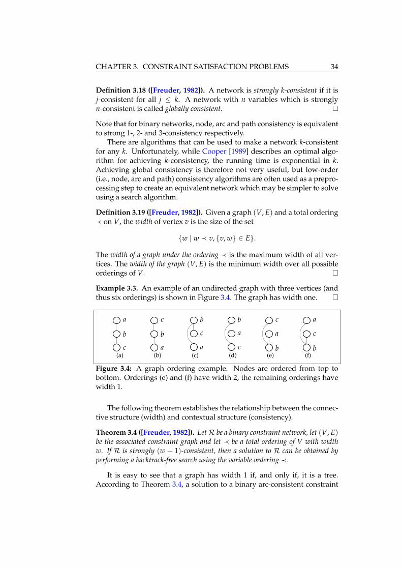
Definition 3.19 ([Freuder, 1982]). Given a graph (V, E) and a total ordering≺ on V, the width of vertex v is the size of the set
w | w ≺ v, v, w ∈ E.
The width of a graph under the ordering ≺ is the maximum width of all ver-tices. The width of the graph (V, E) is the minimum width over all possibleorderings of V.
Example 3.3. An example of an undirected graph with three vertices (andthus six orderings) is shown in Figure 3.4. The graph has width one.
a
b
c(a)
a
b
c
(b)a
b
c
(c)
a
b
c(d)
a
b
c
(e)
a
b
c
(f)
Figure 3.4: A graph ordering example. Nodes are ordered from top tobottom. Orderings (e) and (f) have width 2, the remaining orderings havewidth 1.
The following theorem establishes the relationship between the connec-tive structure (width) and contextual structure (consistency).
Theorem 3.4 ([Freuder, 1982]). LetR be a binary constraint network, let (V, E)be the associated constraint graph and let ≺ be a total ordering of V with widthw. If R is strongly (w + 1)-consistent, then a solution to R can be obtained byperforming a backtrack-free search using the variable ordering ≺.
It is easy to see that a graph has width 1 if, and only if, it is a tree.According to Theorem 3.4, a solution to a binary arc-consistent constraint

3.4. TRACTABLE PROBLEMS 35
network can therefore be found without backtracking. A width-1 orderingof a tree can be constructed by a breadth first search from any root node.Consider a width-1 ordering of the variables d = x1, . . . , xn and assume aconsistent instantiation a of variables x1, . . . , xi has been found. We nowneed to instantiate xi+1. Since d has width 1, xi+1 has only one parent vari-able xj, 1 ≤ j ≤ i which can constrain xi+1. Since xj is arc consistent relativeto xi+1, there exists a value b ∈ Dxi+1 such that a ∪ 〈xi+1, b〉 is consistent.
It is tempting to believe, that finding the width w of the constraint graphand making the network strongly (w + 1)-consistent is sufficient to ensurethat a solution can be found without backtracking. However, for w > 2enforcing w-consistency generally means that new constraints are added(as was the case in path-consistency), thereby changing the width.
There is some debate as to how much consistency is cost effective. Gen-erally speaking, any search algorithm will benefit from a network having ahigh level of consistency. But achieving a high level of consistency comesat the expense of additional computation, so there is a tradeoff between theeffort spent on preprocessing and the effort spent on search. It was thoughtnot to be cost effective to apply consistency algorithms as part of a hybridsearch algorithm [Kumar, 1992] however, especially for difficult problems,it has become clear that this is not the case [Sabin and Freuder, 1994].

CHAPTER 3. CONSTRAINT SATISFACTION PROBLEMS 36
CHAPTER 4
Interactive ConstraintSatisfaction
The CSP definitions and algorithms presented in the previous chapter arefor batch processing where the machine is intended to solve the problemautonomously. Many real world applications, however, require interactivedecision support rather than automatic problem solving. This is the casewhere the initial constraint network admits many possible solutions andhuman guidance is needed to select a solution based on some additionalcriteria. These criteria cannot be modeled as constraints in the original net-work since they are not yet known — the user can only identify these crite-ria when consequences of the initial constraints are revealed.
In this chapter I first define a list of usability requirements for an inter-active constraint satisfaction system, and proceed with an extension of theclassical CSP framework (presented in Section 3.1) which can be used todescribe interactive constraint satisfaction problems. From these require-ments and definitions, I identify operations that are fundamental for aninteractive constraint satisfaction system and describe them formally. Ef-ficient algorithms for the fundamental operations are then presented. Tomake the algorithms efficient, they do not operate on a general constraintnetwork, but on a restricted network called an acyclic network. In the nextchapter, we will see how a general constraint network can be transformedinto an acyclic network by a compilation procedure.
4.1 Usability Requirements
The setup is this: We are given an initial constraint network that models theproblem at hand and this initial constraint network contains some degrees
37

CHAPTER 4. INTERACTIVE CONSTRAINT SATISFACTION 38
of freedom, i.e., it allows more than one solution. This initial constraint net-work cannot be changed by the user but guided by the user’s requirements,the number of solutions should be reduced until the number of solutionsremaining is manageable or a single solution is found. Note that in thefollowing, the term “user” denotes the person that is using the initial con-straint network to find a set of solutions that match the user’s criteria.
Example 4.1. The n-queen problem can be used as a simple example. Theinitial constraint network models the problem as described in Section 1.1.2on page 3. This network cannot be changed by the user, as it would nolonger model the n-queen problem. However, the initial constraint networkdoes have some degrees of freedom that allow the user to influence thesolution to be found. As an example, for n = 4, the queen in the firstcolumn can be placed in either row 2 or 3 as illustrated in Figure 3.1 onpage 21.
The number of solutions to a constraint satisfaction problem can be re-duced by repeatedly adding constraints to an initial constraint network(since the addition of a constraint never extends the set of solutions to thenetwork). During this process, some users will likely make choices that arewrong, either due to outright errors but more likely because they gain newinsights as they proceed. These wrong choices result either in a networkwith no solutions or with a set of solutions which does not fulfill the cri-teria established by the user. An interactive constraint satisfaction systemmust thus allow for the retraction of already stated constraints.
An initial approach to interactive constraint satisfaction may be to ex-tend a search algorithm with a method for letting the user decide whichvariable to instantiate next and what value to use in the instantiation. This,however, is of little value to the user since the machine is merely used torecording the user’s choice and checking if it is consistent with the initialnetwork and previous choices. If backtracking is needed because a solutiondoes not exists with the current choices, the user has to change one or moreof the choices made earlier.
A more reasonable approach would be to let the user specify a con-straint and reveal the consequences of adding this constraint by updatingthe domains to include only values that, based on the initial network anduser constraints, can be extended to a full solution.
A number of usability requirements for interactive constraint satisfac-tion systems can be listed. Frayman [2001] describes many of the require-ments that one can have to such a system. Many of these requirements per-tain the design of the user interface (i.e., easy navigation, intuitive graphicallayout etc.) or the system architecture (i.e., client vs. server processing, se-curity etc.). We will not focus on these requirements here. Instead I list therequirements that need support from the underlying algorithms and datastructures.

4.1. USABILITY REQUIREMENTS 39
1. When the decision support task is complete, the resulting instantia-tion must be consistent. This requirement is the motivation for imple-menting a constraint-based decision-support system.
2. The user should be able to make a “deselection” stating “this variableshould not have these values”. Often the specific value of a variable isnot interesting, but it is important that it is not assigned a few specificvalues.
3. If the user wishes to make a selection, which is inconsistent with pre-vious selections, the system should provide the user with a list ofprevious selections that need to be retracted in order to make thenew selection consistent. In this way, the user is not locked by previ-ous selections since they can be changed if a specific value of anothervariable is deemed more important.
4. The user should be able to make a selection and later retract the selec-tion. It is a fundamental aspect of a good user interface that the useris able to undo actions since this allows experimenting with actionswithout any risk.
5. The user must be able to make selections in arbitrary order. Again thisis a fundamental aspect of a good user interface that the sequence inwhich things are selected is not fixed. Different users may prefer todo things in different orders.
6. The user should not be able to make selections that lead to a dead-end, i.e., a situation where a solution cannot be found because of theselections made earlier in the process. A dead-end in the 4-queenproblem is depicted in Figure 3.1(c) on page 21. Assume the userhas manually selected the position of the three first queens. Theseselections are all mutually consistent, however, it is not possible tomake a consistent selection for the last queen, and thereby completingthe decision task, without changing some of the previous selections.
7. The response time for all operations should be short. An operationshould take less than 1 second for the user’s flow of thought to stayuninterrupted [Nielsen, 1994, Ch. 5]. The limit for keeping the user’sattention focused on the dialogue is about 10 seconds.
The requirement to the response time should of course be seen in perspec-tive to the size of the problem one is attempting to solve. If the user is tryingto solve a problem that would have required weeks of manual work, it maybe acceptable to wait a few minutes for the operations to be completed.

CHAPTER 4. INTERACTIVE CONSTRAINT SATISFACTION 40
4.2 Extension of the Classical CSP Framework
The preceding concepts are formalized in the following definitions where Idescribe an extension of the classical CSP framework, which can be usedto describe interactive constraint satisfaction problems. The notation isinspired by [Amilhastre et al., 2002], and separates a set of dynamic con-straints from the initial constraint network.
Definition 4.1 (Dynamic Constraint Network). A dynamic constraint net-work (DCN) is a 4-tuple ∆ = (X, D, C, H) where (X, D, C) is a satisfiableconstraint network with a static set of variables X, domains D and a staticset of constraints C. The set H is a dynamic set of constraints on the vari-ables X.
As with the constraints in C, we assume that constraints in H have uniquescopes.
Definition 4.2. An instantiation a is a solution to a DCN ∆ = (X, D, C, H)if, and only if, a is a solution to the constraint network (X, D, C ∪ H). Theset of all solutions to ∆ is denoted Sol(∆). The DCN ∆ is satisfiable (respec-tively unsatisfiable) if, and only if, the constraint network (X, D, C ∪ H) issatisfiable (respectively unsatisfiable).
Definition 4.3. Let ∆ = (X, D, C, H) be a DCN, S ⊆ X a set of variables andCS a constraint on S such that (X, D, C ∪ CS) is a satisfiable constraintnetwork. A restoration of CS on ∆ is a subset E ⊆ H such that (X, D, C ∪E ∪ CS) is a satisfiable constraint network. A restoration E of CS on ∆is maximal if, and only if, there is no restoration E′ of CS on ∆ such thatE ⊂ E′.
When combining sets of constraints in Definitions 4.2 and 4.3 we takethis to mean that for any two constraints with the same scope, only a singleconstraint, which is the intersection between the two constraints, is presentin the combined set. A constraint in H is called a user constraint, userselection, or just selection.
For the sake of generality, these definitions do not restrict the type ofdynamic constraints in H. I will assume, however, that these constraintsare always unary. As we will see, this restriction enables efficient algo-rithms for the fundamental operations while being sufficient to fulfill therequirements stated in Section 4.1 on page 37. Assigning a specific valueto a variable can be expressed by adding a unary constraint, which allowsonly that specific value, on the variable.
The goal of interactive constraint satisfaction is, given a dynamic con-straint network ∆ = (X, D, C, H) where H is initially empty, to repeatedlyadd constraints to H until |Sol(∆)| ≤ γ for some constant γ which is thenumber of possible solutions the user can cope with. In many applicationsγ = 1 meaning that a single unique solution must be found.

4.2. EXTENSION OF THE CLASSICAL CSP FRAMEWORK 41
4.2.1 Implications of Usability Requirements
By using the preceding definitions, we can describe the implications of theusability requirements (described in Section 4.1), on the fundamental op-erations required in an interactive constraint satisfaction system. We willuse a DCN ∆ = (X, D, C, H) to capture the initial constraint network (asspecified by X, D and C) as well as the user selections (stored in H).
• Requirement 1 implies that we only return consistent instantiations,i.e., solutions to ∆.
• According to Requirement 2, the values that should not be selectedfor a variable x are in a set Nx ⊂ Dx. We can then fulfill the require-ment by adding the constraint Cx = Dx − Nx to H, which allows alldomain values except the values that are not wanted.
• When the user wishes to add an inconsistent constraint Cx to H, Re-quirement 3 implies that a restoration E of Cx on ∆ is computed. Theselections that need to be retracted are thus H − E. Note that E is notrequired to be maximal.
• Selection and retraction in Requirement 4 can be achieved by adding/removing a constraint to/from H.
• Requirement 5 is implicit in our choice of representing selections as aset of constraints. It does imply, however, that we cannot rely on anyfixed variable ordering in our algorithms.
• Requirement 6 implies that global consistency (as defined in Defini-tion 3.18 on page 34) should be maintained at all times. Having aglobally consistent network means that whenever we have instanti-ated k− 1 variables, we can always find a consistent value for any ofthe remaining variables and this holds for all k < n.
Restoration Computation
As noted, the restoration computed as a result of adding an inconsistentconstraint need not be maximal. Indeed, the trivial restoration ∅ will suf-fice, but in this case all user selections are retracted which is probably notthe best solution. By changing how the restoration is computed, a numberof different behaviors can be achieved.
• From a usability perspective we can argue that the user probablymakes selections in decreasing order of importance. By storing thedynamic constraints in H as an ordered list, we can thus compute therestoration by first removing all constraints from H and then add asmany constraints as possible, starting from the beginning of the list.

CHAPTER 4. INTERACTIVE CONSTRAINT SATISFACTION 42
• By defining a valuation function θ : H → N, a degree of impor-tance can be attached to each dynamic constraint. If we let θ(E) =∑Cx∈H−E θ(Cx), the restoration E computed should be maximal in thesense that there is no restoration E′ satisfying θ(E′) < θ(E).
Note that the behavior of the first method can be achieved by using thesecond method and defining θ appropriately. It is likely, however, that thecomplexity of the two methods is different
4.3 Fundamental Operations
We are now in a position where we can describe the fundamental opera-tions needed in an interactive constraint satisfaction system. In the follow-ing, D is a function constructed from the function D such that
D(x) ⊆ D(x), for all x ∈ X, (4.1)
and D = ∅ is used to denote the function D where
D(x) = ∅, for all x ∈ X. (4.2)
The basic idea is as follows. The initial constraint network is stored in(X, D, C). Modifications to the domains, due to addition/removal of con-straints to/from H, are recorded in D. By comparing values of D before andafter one of the operations, it is possible to compute the changes caused bythe addition/removal of a constraint.
ADD-CONSTRAINT(∆, Cx) → (D, H)
Input: ∆ = (X, D, C, H) is a DCN and Cx a unary constraint.Output: A function D, and a set of constraints H.Precondition: There is no Cy ∈ H such that y = x.Postcondition: If (X, D, C, H∪Cx) is unsatisfiable then H = H and
D = ∅. Otherwise, H = H ∪ Cx, and D is a function where
D(y) = πy(Sol(X, D, C, H)), for all y ∈ X. (4.3)
REMOVE-CONSTRAINT(∆, x) → (D, H)
Input: ∆ = (X, D, C, H) is a DCN and x ∈ X a variable.Output: A function D, and a set of constraints H.Precondition: There exists Cy ∈ H such that y = x.Postcondition: H = H − Cx. D is a function where
D(y) = πy(Sol(X, D, C, H)), for all y ∈ X. (4.4)
RESTORATION(∆, Cx) → E

4.4. APPLICATION TO CONSTRAINT-BASED CONFIGURATION 43
Input: ∆ = (X, D, C, H) is a DCN and Cx a unary constraint.Output: E a restoration of Cx on ∆ or ∅.Precondition: (X, D, C, H ∪ Cx) is unsatisfiable.Postcondition: If (X, D, C, Cx) is satisfiable, E is a restoration of Cx
on ∆, otherwise E is ∅.
Equations (4.3) and (4.4) imply that upon return from ADD-CONSTRAINT
and REMOVE-CONSTRAINT, the domain values in D can be used to extendthe current instantiation to a full solution without having to change anyprevious selections.
By using these fundamental operations it is possible to create an inter-active constraint solver. The skeleton of such a solver is shown in Algo-rithm 4.1 on the following page. Lines 12–18 deal with the selection of aninconsistent value by computing the restoration, removing the constraintsthat cause the inconsistency and finally applying the new selection.
If we assume that line 4 does not involve any complicated rendering ofthe variables the response time of the UI is clearly dominated by the run-ning times of ADD-CONSTRAINT, REMOVE-CONSTRAINT, and RESTORA-TION. Of these three algorithms, ADD-CONSTRAINT is probably the mostoften used, since REMOVE-CONSTRAINT is only called when the user wishesto remove a previous selection and RESTORATION is called when the usermakes a selection that is inconsistent with the previous selections.
4.4 Application to Constraint-Based Configuration
We have already seen configuration problems in Section 1.2 on page 6. HereI will briefly describe how an interactive constraint satisfaction system canbe used as a basis for a configuration system.
As noted, a configuration model is used to describe the components thatare available as well as the relations between them. It is therefore naturalto define the configuration model in terms of a constraint network:
Definition 4.4 (Configuration Model). A configuration model is a constraintnetwork R = (X, D, C). The variables in X list the components availablefor selection, the domains in D contain the possible choices for each com-ponent and the constraints in C contain the constraints between the com-ponents.
The goal of the configuration task is to solve a configuration problemdescribed by a configuration model. Starting with a product model withmany possible solutions, the user gradually reduces the number of solu-tions by choosing consistent values from the variable domains. The con-figuration system should assist the user by resolving which domain valueslead to consistent assignments.

CHAPTER 4. INTERACTIVE CONSTRAINT SATISFACTION 44
SOLVER(X, D, C)1 (D, H) ← (D, ∅)2 ∆ ← (X, D, C, H)3 repeat4 Print available variables and valid domain values from D5 Read user input6 if input = “quit”7 return8 else if input = select value a for variable x9 Cx ← a
10 (D, H) ← ADD-CONSTRAINT(∆, Cx)11 if D = ∅12 E ← RESTORATION(∆, Cx)13 if E = ∅14 error “Invalid selection”15 else if User accepts retraction of the constraints H − E16 for each Cy ∈ H − E17 REMOVE-CONSTRAINT(∆, y)18 (D, H) ← ADD-CONSTRAINT(∆, Cx)19 else if input = remove selection on variable x20 (D, H) ← REMOVE-CONSTRAINT(∆, x)21 else22 error “unknown input”23 until |Sol(X, D, C, H)| < γ
Algorithm 4.1: A skeleton interactive constraint solver using the funda-mental operations.
An instance of a configuration problem can be represented by a DCN∆ = (X, D, C, H). The product model is a constraint network (X, D, C) andthe user restrictions are the set of dynamic constraints H. With this defini-tion each solution to (X, D, C) represents a feasible product1. At any time,Sol(∆) corresponds to the set of feasible products that satisfy the user’srequirements. The generic interactive constraint solver shown in Algo-rithm 4.1 can be used as basis for the runtime services in a configurationsystem, as illustrated in Figure 1.4 on page 8.
Example 4.2. Let the product model be defined by the constraint networkin Example 3.2 on page 23. Initially, when H = , all domain valuesare possible. Now the user decides she wants a desktop model by addingthe constraint Ccase = desktop. We update the list of domain valuesaccording to Equation (4.3) on page 42, and keep the domain values that
1And we can generally assume that (X, D, C) is satisfiable with more than one possiblesolution. Otherwise we would not need a configuration system.

4.4. APPLICATION TO CONSTRAINT-BASED CONFIGURATION 45
are still consistent with the user constraints in H. The changed domainsare
Dide = 40gb, 80gbDscsi = none
As can be seen, there are no choices left for the variable scsi. The valuehas been completely determined by the user constraint. Now we add theconstraint Cmodel = home. The updated domain is:
Dcpu = PIII, AMD
Now the user reconsiders, and decides that she really needs a Pentium IVCPU, i.e., the constraint Ccpu = PIV. This is an inconsistent selectionsince the value PIV is no longer valid for the variable cpu. We thereforecalculate the restoration Ccase. In other words, the user needs to relax theconstraints H − Ccase = Cmodel in order to satisfy the constraint Ccpu.The new domains are:
Dmodel = officeDcase = desktopDide = 40gb, 80gbDscsi = noneDcpu = PIV
The only remaining selection is ide.
In this example it is relatively straightforward to determine which of theprevious selections caused the desired selection to become unavailable. Butfor models containing thousands of variables it is very difficult to manuallyidentify the source of an inconsistent selection.
4.4.1 Model Specification
Creating and specifying a product model is often the most complicated taskin implementing a configuration system. Many practical issues arise whentrying to model a company’s products. Many companies have productfamilies, which contain different products, but share many common com-ponents. To ease maintenance it is therefore essential that product mod-els can be created in a modular fashion, with components shared betweenmodels. A lot of research in configuration involves constructing modeldescription languages [Soininen et al., 2001; Soininen and Niemelä, 1999;Sabin and Freuder, 1996].

CHAPTER 4. INTERACTIVE CONSTRAINT SATISFACTION 46
In this thesis, however, we focus on the configuration task and we there-fore ignore any details of the modeling task, including how the model iscreated. We simply assume the product model is represented by a con-straint network R = (X, D, C), and the constraints in C are representedextensionally as relations. In practice, the last assumption is not an issuesince all constraints on finite domains, whether they are specified as propo-sitional forms, relations or something completely different, can always beconverted into the extensional form used here.
4.4.2 Pros and Cons of Constraint-Based Configuration
Constraint-based methods have many advantages compared to implement-ing a configuration system using a procedural approach:
• Relations between components are specified in a declarative way, i.e.,the modeler states what the relations are, not how they should be en-forced.
• It is usually easy to check if a constraint is correct since there are noside effects and correctness is not influenced by other constraints inthe model2.
• The configuration system can check if the constraints are in contra-diction with each other (by ensuring satisfiability of the model). Thisis useful when changing a model to ensure that the changes are con-sistent with the existing constraints.
• Powerful facilities for the end user can be provided (i.e., restorationsand global consistency). This would be very hard to provide if theconfiguration system was implemented using a traditional program-ming language.
Despite all the advantages, there are a number of issues with constraint-based configuration as presented in this section:
• All domains are finite. In real-world applications we may not know inadvance how large the domains should be, so in order to model theseproblems using a finite domain CSP, we have to make the domainslarger than the largest value we think we will need. Since the sizeof the domains influence the computation time needed to solve theproblem, this may not be feasible.
• The constraints presented here are “hard” in the sense that a solu-tion must always satisfy all the constraints. In some applications, soft
2This requires, of course, that the meaning of a single constraint can be easily under-stood, e.g., by representing it using symbolic logic.
4.5. EFFICIENT FUNDAMENTAL OPERATIONS 47
constraints are needed. Soft constraints are constraints that are notrequired to be satisfied, but are satisfied if possible.
Several researchers have proposed extensions to the classical CSP frame-work in order to cope with these issues (see, e.g., [Mittal and Falkenhainer,1990; Miguel and Shen, 1999] and [Schiex, 1992; Dechter, 1996]). Still, theformulation used in this section is applicable to a large number of practi-cal cases and has been used as the foundation of at least one commercialconfiguration product [Yu and Skovgaard, 1998].
4.5 Efficient Fundamental Operations
In the previous sections we ignored the complexity of the fundamental op-erations. Both ADD-CONSTRAINT and RESTORATION must solve a CON-STRAINT SATISFIABILITY problem which was provedNP-complete in The-orem 3.2 on page 26. This makes them unsuitable for interactive use whenapplied to general constraint networks.
We will, however, postpone the treatment of general networks to thenext chapter. For now, we assume the initial network has a certain structurewhich allows efficient implementation of the fundamental operations. Inthe next chapter, we will see how any general constraint network can betransformed into a network having this structure called an acyclic network.
Definition 4.5 (Acyclic Network). Let R = (X, D, C) be a constraint net-work. An acyclic network for R is a constraint network R = (X, D, C) suchthat X ⊆ X, D ⊆ D satisfying the following properties:
1. When restricted to the variables in X, the two networks have the sameset of solutions, that is
Sol(R) = πX(Sol(R). (4.5)
2. The constraint graph of the dual network of R form a tree if redun-dant constraints are removed.
This definition allows us to add variables to the network and change theconstraints if we ensure the two properties hold. The first property ensuresthat a solution to R is also a solution to the original network R. The sec-ond property ensures that we can process the network efficiently if we usethe dual network representation of R. The dual network is always binaryand a tree has width 1; so according to Theorem 3.4 on page 34, we cansolve the problem without backtracking by enforcing arc consistency (andusing, e.g, the ordering obtained by performing a breadth-first search onthe constraint graph of the dual network).
If we choose to add variables to the problem, they should, of course,not be visible to the end user who is only interested in the variables of theoriginal network.

CHAPTER 4. INTERACTIVE CONSTRAINT SATISFACTION 48
4.5.1 Fundamental Operations on an Acyclic Network
Having identified the structure which we are working with, we need todescribe how the fundamental operations (which operate on the originalnetwork) map to the acyclic dual network.
In the following, we assume the initial network is R = (X, D, C). Thevariables and domains of the acyclic dual network are Xd and Dd respec-tively, both defined as in Definition 3.11 on page 22. Let us first make a fewobservations.
Lemma 4.1. Let R be an acyclic network and Rd = (Xd, Dd, Cd) the correspond-ing dual network. If Rd is arc consistent, then R is satisfiable if, and only if, alldual domains are non-empty. That is,
|Sol(R)| > 0 ⇐⇒ DdR 6= ∅, for all R ∈ Xd, Dd
R ∈ Dd. (4.6)
Proof. First we note that, by definition, R is satisfiable if and only if Rd issatisfiable.
If a dual domain is empty then Rd is clearly unsatisfiable. Assumetherefore that all dual domains are non-empty. A solution to Rd can befound as follows. Assign a valid value to an arbitrary dual variable R.Since Rd is arc consistent, we can assign a consistent value for all dual vari-ables adjacent to R. We can repeat this step, yielding a breadth-first searchin the constraint graph of Rd, until we have assigned valid values for alldual variables. Since the constraint graph of Rd is a tree, we never have toselect a value which makes a previous assignment inconsistent.
Note that the reverse implication holds even if Rd is not arc consistent: Ifany dual domain becomes empty, R is unsatisfiable.
Lemma 4.2. Let R be an acyclic network and Rd = (Xd, Dd, Cd) the correspond-ing dual network. If Rd is arc consistent, then all dual variables Xd agree on thevalues of the original variables in X. That is,
πx(DdR) = πx(Dd
S), for all R, S ∈ Xd and x ∈ R ∩ S. (4.7)
Proof. Let R and S be two dual variables sharing at least one original vari-able. Furthermore, let R and S by connected by a constraint in the con-straint graph of Rd. Since Rd is assumed to be arc consistent, for each tuplet ∈ Dd
R, we can find a tuple u ∈ DdS such that t|R∩S = u|R∩S since this is the
only constraint between R and S according to Definition 3.11 on page 22.We can similarly, for each tuple in u ∈ Dd
S, find a tuple t ∈ DdR satisfying
the same condition. In other words, we have
πR∩S(DdR) = πR∩S(Dd
S) (4.8)
in particular R and S agree on every shared original variable x ∈ R ∩ S.

4.5. EFFICIENT FUNDAMENTAL OPERATIONS 49
By Definition 4.5, all dual variables Sk, . . . , S` ⊆ Xd sharing an origi-nal variable x ∈ X are connected by a path of constraints. By applying theprevious argument to each pair of dual variables we get
πx(DdSk
) = · · · = πx(DdS`
), (4.9)
which proves the lemma.
Adding a constraint CS to an acyclic network R = (X, D, C) will, ingeneral, change the constraint graph of the dual network, in which case itmay no longer have width 1. In the special case where all variables in Sare covered by constraints, i.e., S ⊆
⋃CR∈C R, it is possible to add the con-
straint without changing the constraint graph of the dual network, by re-moving from the domains in Rd values that do not satisfy CS. In constraintnetworks arising from practical problems, we can usually assume that allvariables are covered by at least one constraint (since otherwise, why is thevariable included in the first place). We will, however, restrict the dynamicconstraints to be unary since this is sufficient to express assignment of val-ues to variables and they have the following desirable properties:
• Adding a unary constraint Cx to R implies that we should removefrom the domain of all dual variables in Rd the tuples that do notsatisfy Cx, i.e., from all dual variables, which contain x, the tuplesthat contain the values Dx −Cx for the variable x should be removed:
DdS ← Dd
S 1 Cx, for all DdS such that x ∈ S. (4.10)
If x is not covered by a constraint in C, we can simply update Dxdirectly:
Dx ← Cx. (4.11)
• Adding a unary constraint to R does not change the structure of thedual constraint graph. This is obvious since we do not introduce anynew dual variables or dual constraints, but merely update the do-mains of the existing dual variables.
After a constraint has been added, the acyclic dual network may not bearc consistent so we need to apply an arc-consistency algorithm in orderto restore arc consistency. Lemma 4.2 implies that, after arc consistencyhas been restored, the dual variables all agree on the value of the originalvariables. Therefore (4.10) can simply be reduced to
DdS ← Dd
S 1 Cx, for some DdS such that x ∈ S. (4.12)
CHAPTER 4. INTERACTIVE CONSTRAINT SATISFACTION 50
The arc consistency algorithm will ensure that the changes will be propa-gated to the remaining domains. The same reasoning can be used to deter-mine the valid domain of the original variable x based on the valid domainsin the dual network:
Dx ← πx(DdS), for some Dd
S such that x ∈ S. (4.13)
In the preceding discussion we ignored the fact that we also need theability to remove constraints, which generally implies that we need to rein-troduce some valid domain values from the initial acyclic dual network.Therefore, actually removing invalid domain values does not seem like agood idea. Instead we will mark the values that are valid and remove thismark if a value becomes invalid. If we, at some later point, need to reintro-duce a domain value due to removal of a user selection, we simply markthe value as valid. We never need to introduce more domain values thanare defined in the original network.
4.5.2 Auxiliary Algorithms
The algorithms for the fundamental operations rely on a number of auxil-iary algorithms, which will be described next. In what follows, the inputnetwork is denoted byR = (X, D, C) and it is assumed that the acyclic net-work R and the acyclic dual network Rd are available. Note that for theDCN ∆ = (X, D, C, H), the constraints in H, which we have assumed areunary, are implicitly reflected in the valid domains of R.
For the complexity analysis we use n, e, d, t, nd, ed, dd, and td to denotethe number of variables, constraints, domain values in the largest domain,and tuples in the largest constraint respectively, for R and Rd. In addition,s will be used to denote the largest number of original variables used by adual constraint, i.e.,
s = maxCd
ST∈Cd|S ∩ T|. (4.14)
We can use the following observations to simplify the results:
n ≤ n, (4.15)
d ≤ d (4.16)
dd = t, (4.17)
nd = e (4.18)
ed ≤ e. (4.19)
Equations (4.15) and (4.16) follow from Definition 4.5, Equations (4.17) and(4.18) from Definition 3.11, and Equation (4.19) follows from Equation (4.18)and the fact that the constraint graph of the acyclic dual network is a tree.
From a complexity perspective we can assume the following:

4.5. EFFICIENT FUNDAMENTAL OPERATIONS 51
• For any variable x the initial domain Dx is a non-empty finite set, sowe can view the domain as integers in the range 1, . . . , |Dx|. Eachdomain value thus requires dlog2|Dx|e bits.
• We can augment each domain Dx with an extra data structure Mx,which is a sequence of |Dx| bits, which is used to mark the valid/in-valid domain values. Initially M[1..|Dx|] = 1. Access and updateto/of a bit takes time O(1). The storage requirement for Mx is |Dx|bits.
• Removing a domain value, i.e. Dx ← Dx−j, j ∈ Dx is implementedas M[j] = 0 which takes time O(1).
• Reintroducing a domain value, i.e. Dx ← Dx ∪ j, j ∈ Dx is imple-mented as M[j] = 1 which takes time O(1).
• The size of a set can be returned in timeO(1) by maintaining countersappropriately.
• The storage requirement for storing a domain Dx is |Dx|+ dlog2|Dx|ebits. We will ignore any additional space needed to map the integersin Dx back to the original values. The initialization time is O(|Dx|) toinitialize Mx.
• The set of variables is finite and static so we can similarly view thevariables as integers in the range 1, . . . , |X|. The function D fromvariables to domains can thus be viewed as an ordered sequence of|X| sets. Updating the function for variable x ∈ X is implemented asan update of the set stored at D[x] which takes time O(1).
Revise-Dual
The algorithm REVISE-DUAL, which is shown in Algorithm 4.2 on the fol-lowing page, takes an acyclic dual network Rd and a unary constraint Cxand updates a domain in Rd to reflect the unary constraint. The domain isupdated according to Equation (4.12) by marking the tuples which do notagree with Cx on the variable x as invalid. The return value is FALSE if thedomain becomes empty (which means that (X, D, C, H ∪ Cx) is unsatis-fiable), otherwise the return value is TRUE. The acyclic dual network is, ingeneral, not arc consistent upon return from REVISE-DUAL.
Lemma 4.3. Let DdS ∈ Dd be the domain of a dual variable S such that x ∈ S.
Then REVISE-DUAL
1. correctly computes DdS ← Dd
S 1 Cx,
2. returns FALSE if DdS is empty after the computation and TRUE otherwise,
and

CHAPTER 4. INTERACTIVE CONSTRAINT SATISFACTION 52
REVISE-DUAL(Rd, Cx)1 Dd
S ← some domain in Rd such that x ∈ S2 r ← FALSE
3 for j ← 1 to|DdS|
4 if MdS[j] = 1
5 if DdS[j]|x ∈ Cx
6 r ← TRUE
7 else8 Md
S[j] ← 09 return r
Algorithm 4.2: Revise domain of a dual variable in Rd to reflect unaryconstraint Cx.
3. has time complexity O(d + t) and space complexity O(d).
Proof. The first part follows from the fact that all valid values in DdS are
checked against Cx and marked invalid if not present. TRUE is returned if,and only if, there is an index value j such that Md
S[j] = 1 and DdS[j]|x ∈ Cx.
This proves the second part. The membership test in line 5 takes time O(1)if we use O(d) time to create a lookup table for the allowed values in Cx.The time complexity is thus O(d + dd), and by using Equation (4.17) wehave proven the third part.
Valid-Domains
The algorithm VALID-DOMAINS, shown in Algorithm 4.3 on the next page,takes a DCN ∆ and creates the set of valid domain values from the domainvalues in the acyclic dual network Rd according to Equation (4.13).
Lemma 4.4. Let ∆ = (X, D, C, H) be a dynamic constraint network and R =(X, D, C) the acyclic network corresponding to (X, D, C). Furthermore, let Rd
be the dual acyclic network obtained from R = (X, D, C) by applying REVISE-DUAL for each unary constraint in H. If Rd is satisfiable and arc consistent thenVALID-DOMAINS
1. returns a function D such that
D(y) = πy(Sol(∆)), for all y ∈ X, and (4.20)
2. has time complexity O(n(d + t)) and space complexity O(d).
Proof. We first note that VALID-DOMAINS treats each variable indepen-dently so it is sufficient to prove the first part for some variable y ∈ X.Second if y is not covered by any constraint in C, the first part is triviallytrue because of lines 14–15. Otherwise, let Dd
S be a domain in Dd such that

4.5. EFFICIENT FUNDAMENTAL OPERATIONS 53
VALID-DOMAINS(∆)1 D ← ∅2 for each y ∈ X3 if there exists some domain Dd
S in Rd such that y ∈ S4 . Compute My5 My[1..|Dy|] = 06 Dy ← ∅7 for j ← 1 to|Dd
S|8 if Md
S[j] = 19 v ← Dd
S[j]|y10 if My[v] = 011 My[v] ← 112 Dy ← Dy ∪ v13 else14 if there exists a Cy ∈ H15 Dy ← Dy ∩ Cy16 D[y] ← Dy17 return D
Algorithm 4.3: Compute valid domains in ∆ from Rd.
y ∈ S. Lines 5–12 compute Dy from DdS. By Lemma 4.2 the dual variables
which contain y all agree on the valid values. It is therefore sufficient toprove that πy(Dd
S) = πy(Sol(∆)).If a ∈ πy(Sol(∆)) then clearly a ∈ πy(Dd
S). Now let b ∈ πy(DdS). Then
b ∈ πy(Sol(∆)), since we can find a solution containing 〈y, b〉 by perform-ing a breadth-first search in the tree rooted at S. Rd is arc-consistent andsatisfiable so we can always find a consistent value for each dual variableencountered during the search. This proves the first part.
Line 5 takes O(d) to initialize My which has size O(d), all the remain-ing operations take O(1) so the time complexity is O(n(d + dd)). UsingEquation (4.17) we have proven the second part.
Arc-Consistency
While the AC-4 arc consistency algorithm has an optimal worst-case timecomplexity and thus better than AC-3, AC-3 usually has better average casetime complexity and is therefore often the algorithm of choice in actual im-plementations [Wallace, 1993]. Bessière and Régin [2001] described a newarc consistency algorithm called AC-2001, which is a refinement of AC-3that has the optimal worst-case time complexity. AC-2001 preserves muchof the simplicity in AC-3, which makes it much simpler to implement com-pared to the other optimal algorithms, AC-4 and AC-6. Bessière and Régin

CHAPTER 4. INTERACTIVE CONSTRAINT SATISFACTION 54
[2001] also presented experimental results that showed improved perfor-mance of AC-2001, for both number of constraint checks and CPU time,when compared with AC-3 and AC-4. They note however, that for prob-lem instances which require a lot of constraint propagation3 the much morecomplex algorithm AC-6, relying on sophisticated data structures, is moreefficient.
The algorithm ARC-CONSISTENCY, which is shown in Algorithm 4.6 onthe facing page, tries to enforce arc consistency in Rd by using techniquessimilar to those in AC-2001 but is adapted here to work with the implicitequality constraints present in the dual network.
The algorithm needs an ordering on the domain values. The domainvalues in the dual network are tuples in a relation, which provides a naturalordering (cf., Section 2.2.1 on page 15). The basic idea is as follows. Foreach dual constraint Cd
S,T the structure Last[S, i, T] contains the index ofthe last tuple in Dd
T which was found as support for the ith tuple in DdS.
Likewise, Last[T, j, S] contains the index of the last tuple in DdS which was
found as support for the jth tuple in DdT. Initially the index is 0 indicating
that no support has been found yet. Whenever we check an arc in the callREVISE-2001(S, T) we can simply, for each ith tuple in S that is still valid,check if the tuple at Last[S, i, T] is still valid in T (lines 3–5). If it is valid,the ith tuple is still valid and we can continue with the next tuple. If it isnot valid, we only need to check the tuples in T that follow Last[S, i, T],since the tuples before have already been checked (lines 6–12). If we finda supporting tuple, we update Last and continue. Otherwise we need tomark the ith tuple of S as invalid since it no longer has support in T.
In ARC-CONSISTENCY,Q is a set of dual variables which have had theirdomains modified (and we thus need to check, for each dual variable S ∈Q, the domains of the dual variables connected to S with a dual constraint,cf., Definition 3.15 on page 29). Initially we check all dual constraints andadd to Q the dual variables with modified domains. PROPAGATION is thencalled to propagate the changes to the remaining variables.
Lemma 4.5. Let Rd be an acyclic dual network.
1. If Rd is unsatisfiable, the return value of ARC-CONSISTENCY is FALSE.
2. If Rd is satisfiable, Rd is made arc consistent and the return value of ARC-CONSISTENCY is TRUE.
3. The time complexity of ARC-CONSISTENCY isO(set2) and space complex-ity is O(et).
3These are usually randomly generated problem instances that fall in the phase tran-sition of arc consistency. See [Gent et al., 1997] for more detail on the phase transitionbehaviour of arc consistency.

4.5. EFFICIENT FUNDAMENTAL OPERATIONS 55
REVISE-2001(S, T)1 changed ← FALSE
2 for i ← 1 to |DdS|
3 if MdS[i] = 1
4 j ← Last[S, i, T]5 if j = 0 ∨ Md
T [j] = 06 k ← j + 17 while k ≤ |Dd
T | ∧ Last[S, i, T] = j8 if Md
T [k] = 1 ∧ MdS[i]|S∩T = Md
T [k]|S∩T9 Last[S, i, T] ← k
10 k ← k + 111 if Last[S, i, T] = j12 Md
S[i] ← 013 changed ← TRUE
14 return changed
Algorithm 4.4: Remove values from DdS without support from Dd
T.
PROPAGATION(Rd,Q)1 while Q 6= ∅2 T ← some dual variable from Q3 Q ← Q− T4 for each S ∈ Xd such that Cd
ST ∈ Cd
5 if REVISE-2001(S, T)6 if Dd
S = ∅7 return FALSE
8 Q ← Q∪ S9 return TRUE
Algorithm 4.5: Propagate changes for dual variables in Q.
ARC-CONSISTENCY(Rd)1 Q ← ∅2 Last[x, y, z] ← 0 for all x, y, z3 for each S ∈ Xd
4 for each T ∈ Xd such that CdST ∈ Cd
5 if REVISE-2001(S, T)6 if Dd
S = ∅7 return FALSE
8 Q ← Q∪ S9 return PROPAGATE(Rd,Q)
Algorithm 4.6: Enforce arc-consistency in Rd.

CHAPTER 4. INTERACTIVE CONSTRAINT SATISFACTION 56
Proof. We first note that ARC-CONSISTENCY only returns FALSE if a dualdomain becomes empty (lines 6–7 of ARC-CONSISTENCY and PROPAGA-TION). To prove the two first parts, it is, according to Lemma 4.1 on page 48,sufficient to prove that Rd is arc consistent when we reach line 9 of PROP-AGATION.
We first claim that REVISE-2001 makes S arc consistent relative to T andreturns TRUE if and only if the domain of S has changed. This follows fromthe fact that all valid domain values in Dd
S are checked (lines 2− 3). If thesupport for a valid domain value is still valid in Dd
T nothing happens (line5). If this is the first call to REVISE-2001 for S and T or if the support hasbeen marked invalid, a new support value is searched in the valid valuesof Dd
T (lines 6–10). If support is found (line 8) we store the index of thesupport value and nothing is changed in Dd
S for this particular value. If nosupport is found (line 11) we mark the domain value in Dd
S as invalid andchange the return value to TRUE.
For ARC-CONSISTENCY we note that initially all arcs are checked twice(one check in each direction). During the loop (lines 3–8) a variable S isadded to Q whenever its domain has changed (line 8). In a subsequentcall to PROPAGATION, all variables which rely on S for support are thenchecked (lines 4–8). These variables are the only variables that can changedue to changes in the domain of S. It follows from this that Q becomesempty and the loop terminates when no further domain values can be re-moved by the call to REVISE-2001, i.e., arc consistency has been achieved.
For the complexity analysis we first note that a variable is placed inQ whenever its domain has changed. In the worst case, only a single do-main value is removed in the call to REVISE-2001. For any constraint Cd
STREVISE-2001(S, T) is therefore called at most dd times. For any tuple inDd
S, line 4 of REVISE-2001 is thus executed at most dd times. The total timespent in lines 5–11 for a single tuple during the dd calls is O(sdd) since weperform the constraint check in line 9 at most once for each tuple in Dd
T,the number of tuples is bounded by dd and a constraint check takes timeO(s). Since the number of tuples in Dd
S is bounded by dd and there are ed
constraints, the worst-case time complexity becomes O(sed(dd)2). The sizeof the set Q is bounded by nd and we need O(dd) space to store the Lastarray for each dual constraint so the space complexity becomes O(eddd).By using Equations (4.17) and (4.19) we have proven the third part.
4.5.3 Algorithms for the Fundamental Operations
The following sections present algorithms for the fundamental operations.
4.5. EFFICIENT FUNDAMENTAL OPERATIONS 57
Add-Constraint
The fundamental algorithm ADD-CONSTRAINT, which is shown in Algo-rithm 4.7, takes a DCN ∆ and a unary constraint Cx and adds the unaryconstraint as described in Section 4.3 on page 42.
Theorem 4.6. Let ∆ = (X, D, C, H) be a DCN and Cx and unary constraint onsome variable x ∈ X. Then ADD-CONSTRAINT
1. correctly computes the sets H and D as described in Section 4.3, and
2. has a worst-case time complexity of O(n(d + t) + set2) and space complex-ity O(et).
Proof. Both parts of the theorem follow from Lemma 4.3, Lemma 4.4 andLemma 4.5.
ADD-CONSTRAINT(∆, Cx)1 if REVISE-DUAL(Rd, Cx) ∧ ARC-CONSISTENCY(Rd)2 D ← VALID-DOMAINS(∆)3 return (D, H ∪ Cx)4 else5 return (∅, H)
Algorithm 4.7: Adding a unary constraint.
Remove-Constraint
The fundamental algorithm REMOVE-CONSTRAINT, which is shown in Al-gorithm 4.8 on the following page, takes a DCN ∆ and a variable x and re-moves the constraint on Cx as described in Section 4.3 on page 42. It naivelyremoves all constraints in H and then adds the constraints H− Cx. Lines2–4 remove the constraints in H by marking all domain values in Rd asbeing valid. Lines 6–10 add the constraints from H − Cx.
Theorem 4.7. Let ∆ = (X, D, C, H) be a DCN and x some variable in X suchthat there exists a constraint Cx ∈ H. Then REMOVE-CONSTRAINT
1. correctly computes the sets H and D as described in Section 4.3, and
2. has a worst case time complexity ofO(n(d + t) + set2) and space complexityO(et).
Proof. The fact that all constraints in H are removed in lines 2–7 combinedwith Lemma 4.3, Lemma 4.4 and Lemma 4.5 proves both part of the theo-rem.
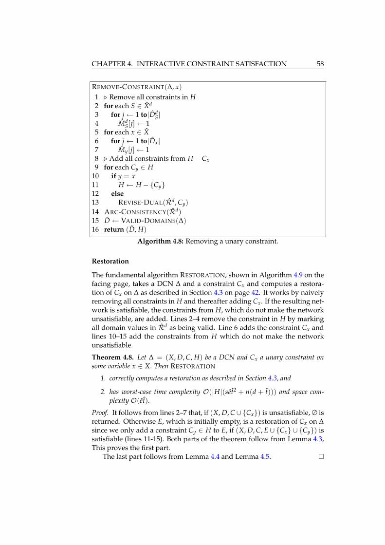
CHAPTER 4. INTERACTIVE CONSTRAINT SATISFACTION 58
REMOVE-CONSTRAINT(∆, x)1 . Remove all constraints in H2 for each S ∈ Xd
3 for j ← 1 to|DdS|
4 MdS[j] ← 1
5 for each x ∈ X6 for j ← 1 to|Dx|7 My[j] ← 18 . Add all constraints from H − Cx9 for each Cy ∈ H
10 if y = x11 H ← H − Cy12 else13 REVISE-DUAL(Rd, Cy)14 ARC-CONSISTENCY(Rd)15 D ← VALID-DOMAINS(∆)16 return (D, H)
Algorithm 4.8: Removing a unary constraint.
Restoration
The fundamental algorithm RESTORATION, shown in Algorithm 4.9 on thefacing page, takes a DCN ∆ and a constraint Cx and computes a restora-tion of Cx on ∆ as described in Section 4.3 on page 42. It works by naivelyremoving all constraints in H and thereafter adding Cx. If the resulting net-work is satisfiable, the constraints from H, which do not make the networkunsatisfiable, are added. Lines 2–4 remove the constraint in H by markingall domain values in Rd as being valid. Line 6 adds the constraint Cx andlines 10–15 add the constraints from H which do not make the networkunsatisfiable.
Theorem 4.8. Let ∆ = (X, D, C, H) be a DCN and Cx a unary constraint onsome variable x ∈ X. Then RESTORATION
1. correctly computes a restoration as described in Section 4.3, and
2. has worst-case time complexity O(|H|(set2 + n(d + t))) and space com-plexity O(et).
Proof. It follows from lines 2–7 that, if (X, D, C ∪ Cx) is unsatisfiable, ∅ isreturned. Otherwise E, which is initially empty, is a restoration of Cx on ∆since we only add a constraint Cy ∈ H to E, if (X, D, C, E ∪ Cx ∪ Cy) issatisfiable (lines 11-15). Both parts of the theorem follow from Lemma 4.3,This proves the first part.
The last part follows from Lemma 4.4 and Lemma 4.5.

4.5. EFFICIENT FUNDAMENTAL OPERATIONS 59
RESTORATION(∆, Cx)1 . Remove all constraints in H2 for each S ∈ Xd
3 for j ← 1to|DdS|
4 MdS[j] ← 1
5 . Add Cx6 if ¬REVISE-DUAL-(Rd, Cx) ∨ ¬ARC-CONSISTENCY(Rd)7 return ∅8 else9 . Add consistent constraints from H
10 E ← ∅11 for each Cy ∈ H12 if REVISE-DUAL(Rd, Cy) ∧ ARC-CONSISTENCY(Rd)13 E ← E ∪ Cy14 else15 REMOVE-CONSTRAINT(∆, Cy)16 return E
Algorithm 4.9: Calculate a restoration.
4.5.4 Summary of Results
Table 4.1 summarizes the complexity results for the fundamental opera-tions. As can be seen, all the fundamental operations can be performed intime polynomial in the size of the acyclic constraint network. This meansthat, given a general constraint network as input, the performance of theseoperations can be assessed when the input network has been transformedinto an acyclic constraint network. Note, however, that the time spent con-structing the acyclic constraint network is, in the worst case, unlikely tobe polynomial in the size of the input network (since otherwise we couldsolve CONSTRAINT SATISFIABILITY in polynomial time, which is unlikelyunless P = NP). The best we can hope for is that the networks that arise inpractical applications can be efficiently transformed into acyclic networks,which have a tractable size.
Function Time Complexity Space Complexity
ADD-CONSTRAINT O(set2 + n(d + t)) O(et)REMOVE-CONSTRAINT O(set2 + n(d + t)) O(et)RESTORATION O(|H|(set2 + n(d + t))) O(et)
Table 4.1: Complexity results for the fundamental operations.

CHAPTER 4. INTERACTIVE CONSTRAINT SATISFACTION 60

CHAPTER 5
Acyclic Network Construction
In the previous chapter, I presented polynomial algorithms for the funda-mental operations in an interactive constraint satisfaction system. The al-gorithms rely on a restricted constraint network called an acyclic constraintnetwork. Requiring that problems must be stated using acyclic networksis too restrictive, so we need a method which can transform a general con-straint network into an acyclic constraint network. This transformation canbe viewed as a compilation of the general network into a form that enablesefficient processing.
Let us first ensure that an acyclic network can be found for any generalconstraint network.
Theorem 5.1. For any general constraint network R = (X, D, C) there exists acorresponding acyclic network.
Proof. Let R = (X, D, C) be a constraint network such that X = X, D = Dand C = CX where CX is the constraint
CX = Sol(R). (5.1)
Then R is an acyclic network for R. It is clear that they have the same setof solutions and since the constraint graph of Rd is a single node, it is atree.
Theorem 5.1 also gives us a method to construct an acyclic network since,as noted in Section 3.1.2 on page 20, the set of all solutions can be found byjoining all the constraints:
CX =1CS∈C CS. (5.2)
61

CHAPTER 5. ACYCLIC NETWORK CONSTRUCTION 62
For networks with a small number of solutions, this method may be accept-able provided that the size of the intermediate results are manageable.
This chapter presents an existing method for synthesizing solutions toa constraint network and an existing method for decomposing a constraintnetwork. We end the chapter by proposing a method for acyclic networkconstruction which combines the two existing methods.
5.1 Array-based Logic
Møller [1995] presented a method for constraint satisfaction based on thetheory of arrays [More, Jr., 1973]. In what follows, the essential parts ofthe method, called array-based logic, are presented using the terminologyalready established in the preceding chapters.
Array-based logic works by basically building the set of all solutions byjoining all the constraints of the network as described in Equation (5.2) onthe page before. As the following example shows, the order in which thejoins of Equation (5.2) are evaluated is important
Example 5.1. In Figure 5.1 on the facing page the relations R, S and T areshown. The join operator is commutative so there are three possible waysin which we can compute the join of these three relations:
(R 1 S) 1 T, (5.3)(S 1 T) 1 R, and (5.4)(T 1 R) 1 S. (5.5)
While all three evaluation orders produce the same result, the size of theintermediate result differs as shown in Figure 5.1. The evaluation orderaccording to Equation (5.5) produces a larger intermediate result than thetwo others, thus it is likely to perform worse.
Møller [1995] used a simple heuristic to select the next pair of con-straints to be joined. For all pairs of constraints CR, CS ∈ C we define theconnectivity factor as
F(CR, CS) = |CR| × |CS| × |R− S| × |S− R|. (5.6)
The connectivity factor should provide an approximation of the size of thejoined result. The intuition behind Equation (5.6) is as follows. The largerthe two constraints, the larger the joined result. This accounts for the firsttwo factors. The more variables shared by the two constraints, the smallerthe result. This accounts for the two last factors. The heuristic simply se-lects the pair of constraints with the smallest connectivity factor as the nextpair to be joined.
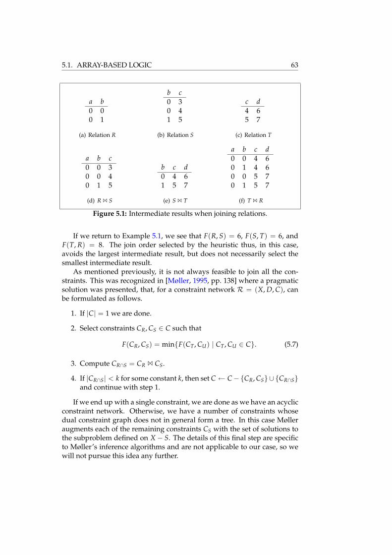
5.1. ARRAY-BASED LOGIC 63
a b0 00 1
(a) Relation R
b c0 30 41 5
(b) Relation S
c d4 65 7
(c) Relation T
a b c0 0 30 0 40 1 5
(d) R 1 S
b c d0 4 61 5 7
(e) S 1 T
a b c d0 0 4 60 1 4 60 0 5 70 1 5 7
(f) T 1 R
Figure 5.1: Intermediate results when joining relations.
If we return to Example 5.1, we see that F(R, S) = 6, F(S, T) = 6, andF(T, R) = 8. The join order selected by the heuristic thus, in this case,avoids the largest intermediate result, but does not necessarily select thesmallest intermediate result.
As mentioned previously, it is not always feasible to join all the con-straints. This was recognized in [Møller, 1995, pp. 138] where a pragmaticsolution was presented, that, for a constraint network R = (X, D, C), canbe formulated as follows.
1. If |C| = 1 we are done.
2. Select constraints CR, CS ∈ C such that
F(CR, CS) = minF(CT, CU) | CT, CU ∈ C. (5.7)
3. Compute CR∩S = CR 1 CS.
4. If |CR∩S| < k for some constant k, then set C ← C−CR, CS ∪ CR∩Sand continue with step 1.
If we end up with a single constraint, we are done as we have an acyclicconstraint network. Otherwise, we have a number of constraints whosedual constraint graph does not in general form a tree. In this case Mølleraugments each of the remaining constraints CS with the set of solutions tothe subproblem defined on X − S. The details of this final step are specificto Møller’s inference algorithms and are not applicable to our case, so wewill not pursue this idea any further.
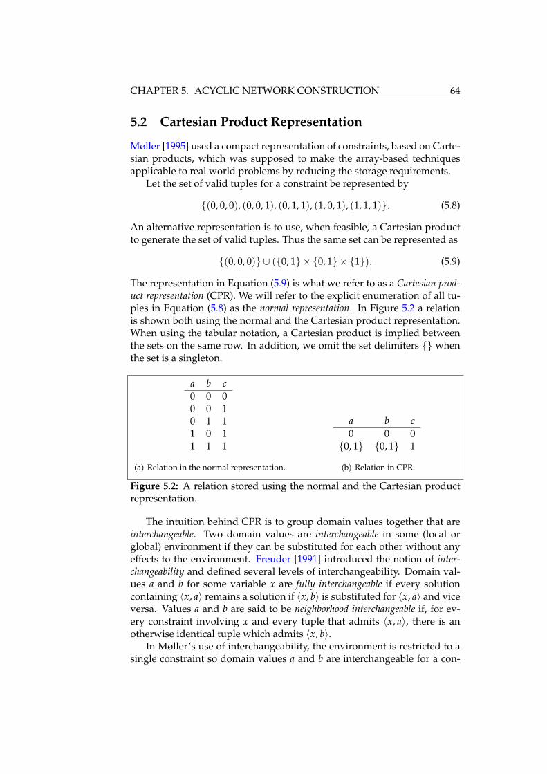
CHAPTER 5. ACYCLIC NETWORK CONSTRUCTION 64
5.2 Cartesian Product Representation
Møller [1995] used a compact representation of constraints, based on Carte-sian products, which was supposed to make the array-based techniquesapplicable to real world problems by reducing the storage requirements.
Let the set of valid tuples for a constraint be represented by
(0, 0, 0), (0, 0, 1), (0, 1, 1), (1, 0, 1), (1, 1, 1). (5.8)
An alternative representation is to use, when feasible, a Cartesian productto generate the set of valid tuples. Thus the same set can be represented as
(0, 0, 0) ∪ (0, 1 × 0, 1 × 1). (5.9)
The representation in Equation (5.9) is what we refer to as a Cartesian prod-uct representation (CPR). We will refer to the explicit enumeration of all tu-ples in Equation (5.8) as the normal representation. In Figure 5.2 a relationis shown both using the normal and the Cartesian product representation.When using the tabular notation, a Cartesian product is implied betweenthe sets on the same row. In addition, we omit the set delimiters whenthe set is a singleton.
a b c0 0 00 0 10 1 11 0 11 1 1
(a) Relation in the normal representation.
a b c0 0 00, 1 0, 1 1
(b) Relation in CPR.
Figure 5.2: A relation stored using the normal and the Cartesian productrepresentation.
The intuition behind CPR is to group domain values together that areinterchangeable. Two domain values are interchangeable in some (local orglobal) environment if they can be substituted for each other without anyeffects to the environment. Freuder [1991] introduced the notion of inter-changeability and defined several levels of interchangeability. Domain val-ues a and b for some variable x are fully interchangeable if every solutioncontaining 〈x, a〉 remains a solution if 〈x, b〉 is substituted for 〈x, a〉 and viceversa. Values a and b are said to be neighborhood interchangeable if, for ev-ery constraint involving x and every tuple that admits 〈x, a〉, there is anotherwise identical tuple which admits 〈x, b〉.
In Møller’s use of interchangeability, the environment is restricted to asingle constraint so domain values a and b are interchangeable for a con-

5.2. CARTESIAN PRODUCT REPRESENTATION 65
straint CS if, for every tuple that admits 〈x, a〉, there is an otherwise identi-cal tuple which admits 〈x, b〉.
Møller used CPR as a way to handle the combinatorial explosion whenjoining constraints, however the use of CPR has also been successfullyapplied to traditional CSP backtracking algorithms [Hubbe and Freuder,1992; Silaghi et al., 1999].
5.2.1 Operations on CPR Relations
The values in a tuple are sets when the constraint is in the CPR and scalarswhen the constraint is in the normal representation. The following defini-tion provides a general way to measure the size of a constraint.
Definition 5.1. The size of a constraint CS with scope S, denoted ‖CS‖, isthe number of scalar values contained in the constraint,
‖CS‖ = ∑x∈S
|CS |
∑i=1|CS[i]|x|. (5.10)
It follows from Definition 5.1 that the size of a constraint CS in the nor-mal representation is equivalent to |S||CS| as would be expected. For aconstraint network R we will use ‖R‖ to denote the total size of all theconstraints in R.
The main benefit of the CPR is that it potentially saves spaces while stillallowing the usual relational operators such as join, project and select to beapplied without having to generate all the tuples of the original constraint.The space savings can be seen in Figure 5.2 on the preceding page wherethe normal representation has size 15 while the CPR has size 8.
The definition of the join operation must be changed slightly to handleCPR constraints. The tuples of two relations should be combined when-ever the intersection between the values of all the common attributes isnonempty. When two tuples are combined, we should only include theintersection of the values from the common attributes. All non-commonattribute values are included as before. Figure 5.3 on the following pageillustrates the result of joining two CPR relations.
This leads to a new definition of the join operator which will also workwith CPR relations. For relations in the normal representation, Defini-tion 5.2 generates the same result as Definition 2.8 on page 14 as wouldbe expected.
Definition 5.2. Let R be a relation with scheme Y and instance r. Let S be arelation with scheme Z and instance s. The join of R and S, denoted R 1 S,

CHAPTER 5. ACYCLIC NETWORK CONSTRUCTION 66
a b c0 0, 1 01, 2 0 1
4 4 1
(a) Relation R.
b c d0, 1 1 1
2 1 31, 3 0 2
(b) Relation S.
a b c d0 1 0 21, 2 0 1 1
(c) R 1 S
Figure 5.3: Joining relations stored using the Cartesian product representa-tion. The two tuples in the result are obtained by combining R[1] with S[3]and R[2] with S[1] respectively.
is defined to be the relation with scheme Y ∪ Z and an instance containingthe following set of tuples:
t = u t v | t is a tuple over Y ∪ Z, u ∈ r, v ∈ s, |u u v| = |Y ∩ Z|, (5.11)
where
u t v = u|Y−Z ∪ v|Z−Y
⋃x∈Y∩X
(u|x ∩ v|x), (5.12)
u u v = x | x ∈ Y ∩ X, u|x ∩ v|x 6= ∅. (5.13)
Equation (5.12) specifies that the new tuple should be combined from all thecomponents of the non-common attributes as well as the intersection of thevalues of the common attributes. Equation (5.13) specifies a set containingcommon attributes where the intersection is not empty. It is easily seenthat Definition 5.2 on the preceding page is equivalent to Definition 2.8on page 14 when joining relations in the normal representation: The lastpart of Equation (5.12) becomes u|Y∩Z and Equation (5.13) becomes a setcontaining the common attributes which have the same value in the twotuples.
Madsen [2002] presented an algorithm for in-memory join of relationsin the CPR. The worst-case running time for joining two relations R and Swith the same scheme is O(|R|‖S‖).
We will introduce a new relational operator to convert a constraint tothe CPR.
Definition 5.3. Let CS be a constraint. The Cartesian product representationof CS is obtained by applying the κ operator on CS. The standard represen-tation is obtained by applying the κ−1 operator. In other words, we have
CS = κ−1(κ(CS)), (5.14)
CS = κ−1(CS). (5.15)

5.3. TREE CLUSTERING 67
For a constraint network R we will use κ(R) to denote the network whereall constraints are in the CPR.
Katajainen and Madsen [2002] presented a heuristic utilizing random-ization for the κ operator. For a constraint CS, the running time of theheuristic is O(|S|2|CS|+ |S||CS| log2 mind, |CS|) in the average case.
5.3 Tree Clustering
Based on results from the theory of relational databases, Dechter and Pearl[1989] presented a general and systematic method of decomposition calledtree clustering. The main idea is to replace the initial constraints with a newset of constraints, that allow the same set of solutions, such that the corre-sponding dual graph forms a tree. This method can thus be used to con-struct an acyclic network.
We start out with some definitions which are adapted here to the termi-nology presented in the preceding chapters.
Definition 5.4. Let G = (V, E) be an undirected graph. G is chordal if everycycle with at least four distinct nodes has an edge joining two non-adjacentnodes in the cycle. Such an edge is called a chord. A hypergraph is chordalif the corresponding primal graph is chordal.
Definition 5.5 ([Berge, 1973]). A hypergraph H = (V, S) is conformal if,for every clique I in the primal graph of H, there is a hyperedge in S thatcontains I.
Definition 5.6 ([Beeri et al., 1983]). For a constraint networkR = (X, D, C)a join tree for R is a tree with a set of nodes C such that
1. each edge CR, CS is labeled by the set of variables R ∩ S, and
2. for every pair CR, CS ∈ C and for every x ∈ R ∩ S each edge along theunique path between CR and CS includes x.
If a join tree exists. it is easy to identify as the following theorem shows.
Theorem 5.2 ([Maier, 1983]). If a constraint network R has a join tree, it is amaximum spanning tree of the dual graph where the edges are weighted with thenumber of shared variables.
Verifying if a constraint network has a join tree can thus be reduced tofinding a maximum spanning tree on the dual graph and verify that thistree satisfies Definition 5.6. Constraint networks that have a join tree canalso be characterized by properties of the constraint hypergraph. This isformalized in Theorem 5.3 on the next page.
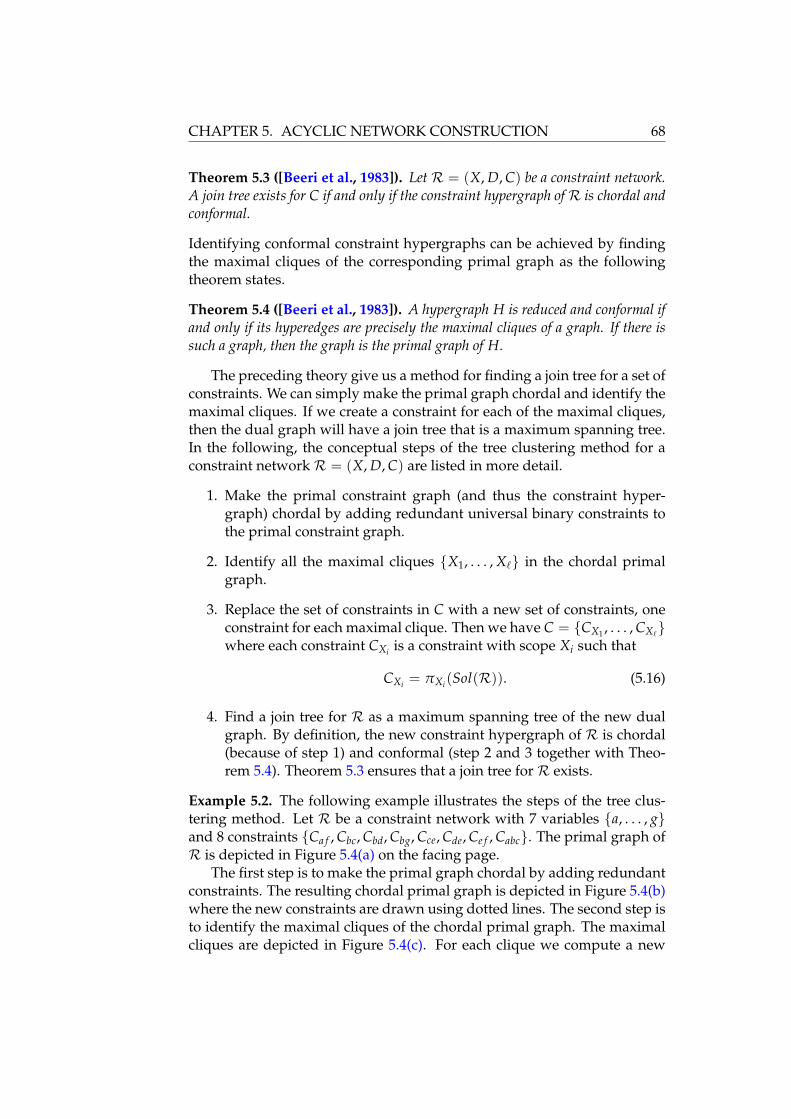
CHAPTER 5. ACYCLIC NETWORK CONSTRUCTION 68
Theorem 5.3 ([Beeri et al., 1983]). Let R = (X, D, C) be a constraint network.A join tree exists for C if and only if the constraint hypergraph ofR is chordal andconformal.
Identifying conformal constraint hypergraphs can be achieved by findingthe maximal cliques of the corresponding primal graph as the followingtheorem states.
Theorem 5.4 ([Beeri et al., 1983]). A hypergraph H is reduced and conformal ifand only if its hyperedges are precisely the maximal cliques of a graph. If there issuch a graph, then the graph is the primal graph of H.
The preceding theory give us a method for finding a join tree for a set ofconstraints. We can simply make the primal graph chordal and identify themaximal cliques. If we create a constraint for each of the maximal cliques,then the dual graph will have a join tree that is a maximum spanning tree.In the following, the conceptual steps of the tree clustering method for aconstraint network R = (X, D, C) are listed in more detail.
1. Make the primal constraint graph (and thus the constraint hyper-graph) chordal by adding redundant universal binary constraints tothe primal constraint graph.
2. Identify all the maximal cliques X1, . . . , X` in the chordal primalgraph.
3. Replace the set of constraints in C with a new set of constraints, oneconstraint for each maximal clique. Then we have C = CX1 , . . . , CX`
where each constraint CXi is a constraint with scope Xi such that
CXi = πXi(Sol(R)). (5.16)
4. Find a join tree for R as a maximum spanning tree of the new dualgraph. By definition, the new constraint hypergraph of R is chordal(because of step 1) and conformal (step 2 and 3 together with Theo-rem 5.4). Theorem 5.3 ensures that a join tree for R exists.
Example 5.2. The following example illustrates the steps of the tree clus-tering method. Let R be a constraint network with 7 variables a, . . . , gand 8 constraints Ca f , Cbc, Cbd, Cbg, Cce, Cde, Ce f , Cabc. The primal graph ofR is depicted in Figure 5.4(a) on the facing page.
The first step is to make the primal graph chordal by adding redundantconstraints. The resulting chordal primal graph is depicted in Figure 5.4(b)where the new constraints are drawn using dotted lines. The second step isto identify the maximal cliques of the chordal primal graph. The maximalcliques are depicted in Figure 5.4(c). For each clique we compute a new
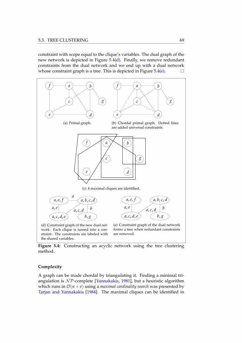
5.3. TREE CLUSTERING 69
constraint with scope equal to the clique’s variables. The dual graph of thenew network is depicted in Figure 5.4(d). Finally, we remove redundantconstraints from the dual network and we end up with a dual networkwhose constraint graph is a tree. This is depicted in Figure 5.4(e).
f a b
c
de
g
(a) Primal graph.
f a b
c
de
g
(b) Chordal primal graph. Dotted linesare added universal constraints.
f a b
c
de
g
(c) 4 maximal cliques are identified.
a, e, f a, b, c, d
a, c, d, e b, g
a
ba, c, da, e
(d) Constraint graph of the new dual net-work. Each clique is turned into a con-straint. The constraints are labeled withthe shared variables.
a, e, f a, b, c, d
a, c, d, e b, g
ba, c, da, e
(e) Constraint graph of the dual networkforms a tree when redundant constraintsare removed.
Figure 5.4: Constructing an acyclic network using the tree clusteringmethod.
Complexity
A graph can be made chordal by triangulating it. Finding a minimal tri-angulation is NP-complete [Yannakakis, 1981], but a heuristic algorithmwhich runs in O(n + e) using a maximal cardinality search was presented byTarjan and Yannakakis [1984]. The maximal cliques can be identified in

CHAPTER 5. ACYCLIC NETWORK CONSTRUCTION 70
time O(e′) where e′ is the number of edges in the chordal graph [Dechterand Pearl, 1989].
Each constraint CXi can be viewed as the set of solutions to the subnet-work defined on the variables in Xi and it thus takes time O(d|Xi |) to findeach constraint. If we let w denote the size of the largest clique, the overallcomplexity is thus exponential in w.
5.3.1 Relation To Tree Decomposition
The tree clustering method described in the previous section fits the generalgraph-theoretic framework of tree decomposition introduced by Robertsonand Seymour [1986].
Definition 5.7. A tree decomposition of an undirected graph G = (V, E) is apair (T,B), where T = (J, F) is a tree and B = Bj | j ∈ J is a family ofsubsets of V such that
1.⋃
j∈J Bj = V,
2. for all v, w ∈ E, there exists a node j ∈ J such that v, w ∈ Bj, and
3. for all x, y, z ∈ J, if y is on the path from x to z in T, then Bx ∩ Bz ⊆ By.
The width of a decomposition (T, Bj | j ∈ J) is maxj∈J |Bj| − 1, and thetreewidth of an undirected graph G, denoted tw(G), is the smallest width ofany tree decomposition of G.
Many NP-complete graph problems can be solved in polynomial timeon graphs which have bounded treewidth. The problem of computing thetreewidth of a graph is in general NP-hard[Arnborg et al., 1987], howeverfor fixed k, linear-time algorithms exist that determine whether a graph hastreewidth at most k, and if so, finds a tree decomposition with width atmost k [Bodlaender, 1996]. Their practical use, however, is limited sincethe running time contains large constants with k in the exponent.
Tree Clustering as Tree Decomposition
The tree clustering method can be seen as a tree decomposition of the dualgraph: Let X1, . . . , X` be the maximal cliques. Then J = 1, . . . , ` andeach subset Bj, j ∈ J corresponds to some maximal clique Xj. Condition 1is clearly satisfied. Every clique is maximal so condition 2 is satisfied. Theresult of tree clustering is a join tree so condition 3 is satisfied. It followsfrom this that the size of the largest clique is then bounded by tw(G) + 1where G denotes the primal graph of the constraint network.
We should note that while the treewidth of a primal constraint graphis an invariant, the size of the largest clique computed by the tree clus-tering method is determined by the heuristics used by the triangulationalgorithm.
5.4. A COMBINED METHOD 71
Other Decomposition Methods
Other decomposition methods have been proposed. Gyssens et al. [1994]present a method called hinge decomposition and they show that the cardi-nality of the largest vertex of any hinge decomposition is an invariant ofthe given network. A hinge tree for a constraint network can be computedin time O(ne2).
Recently, a general hypertree decomposition method has been proposedin database research [Gottlob et al., 1999a]. It is similar to tree decompo-sition, but is now defined on hypergraphs instead of regular undirectedgraphs. As was the case with a tree decomposition, finding a hypertree de-composition with minimum hyperwidth is NP-complete. A polynomialtime algorithm exists for determining whether a hypertree decompositionof hyperwidth at most k exists for any fixed k, and if so, return a hypertreedecomposition of hyperwidth at most k [Gottlob et al., 1999b]. The prac-tical relevance of this remains to be seen, but as was the case with a treedecomposition, the worst-case running time of the hypertree decomposi-tion algorithm is exponential in k.
In [Gottlob et al., 2000] various CSP decomposition methods (includingtree clustering, hinge decomposition, and hypertree decomposition) werecompared. A way of comparing decomposition methods was proposed,in which a method d1 is more powerful than method d2 in the sense thatwhenever d2 guarantees the decomposed problem can be solved in polyno-mial time, the problem decomposed using d1 is also solvable in polynomialtime, but there are classes that can be solved in polynomial time using d1but not d2. The conclusion of the paper was that the hypertree decomposi-tion is the most powerful of the current known methods.
One of the authors of [Gottlob et al., 2000] provides a program1 that canfind a hypertree decomposition of width k if such a decomposition existsand returns failure otherwise. The program was briefly tested on some ofthe constraint network instances used in the performance study presentedin Chapter 6, but due to the memory requirements (k = 3 required 2GBmemory, for k > 3 the program crashed with an overflow error), I did notsucceed in producing any hypertree decompositions.
5.4 A Combined Method for Acyclic Network Con-struction
Both array-based logic and tree clustering construct acyclic networks. How-ever the two methods can also be combined: We can utilize array-based
1At the time of writing it was available at http://si.deis.unical.it/~frank/Hypertrees/ .
CHAPTER 5. ACYCLIC NETWORK CONSTRUCTION 72
logic to solve the subproblems induced by the cliques found by tree clus-tering. Another matter that we have not covered yet is how the CPR affectthe algorithms for the fundamental operations described in Chapter 4 onpage 37. Both of these issues are explained in the following.
5.4.1 Solutions to Subproblems
As noted in Section 5.3 on page 67, the first part of the tree clusteringmethod identifies a number of cliques, each of which induces a subnet-work for which all solutions must be found. We find these constraints asfollows.
1. Place each original constraint CR in a set SXi such that R ⊆ Xi. Eachoriginal constraint CR forms a clique in the primal graph. If this cliqueis not maximal, there exists another clique Xj such that R ⊆ Xj.
2. For each SXi construct a constraint CXi
CXi =
UXi if SXi = ∅,UXi∩ 1CS∈SXi
CS if SXi 6= ∅.(5.17)
Note that the constraints in Equation (5.17) can be tightened further by con-sidering all constraints of the original problem sharing a variable with theclique being processed:
CXi ← CXi ∩ πXi(1CS∈C,S∩Xi 6=∅ CS). (5.18)
5.4.2 Fundamental Operations for CPR Constraints
In a CPR constraint, a single tuple no longer represents a single valid as-signment but instead a set of valid assignments. A tuple in a CPR constraintis thus invalid exactly when all the assignments represented by the tupleare invalid. It is possible to determine the set of tuples in a single CPR con-straint that become invalid because of unary constraints, as the followinglemma shows.
Lemma 5.5. Let S = x1, . . . , x` be a set of variables and let CS be a CPRconstraint on S. Furthermore, let Cxi be a (possibly universal) unary constraintfor each xi ∈ S. The set of tuples that are invalid because of the unary constraintsCxi are exactly those identified by the set
t | t ∈ CS, t|xi∩ Cxi = ∅ for some xi ∈ S. (5.19)
Proof. If t|x ∩ Cxi 6= ∅ for all xi ∈ X, then t clearly represents at least onevalid assignment, namely t|x1 ∩ Cxi × · · · × t|x`
∩ Cx`.

5.4. A COMBINED METHOD 73
As the following lemma shows, it is also possible to determine the op-posite: the set of valid domain values can be determined from the set ofvalid tuples.
Lemma 5.6. Let S = x1, . . . , x` be a set of variables and let CS be a CPRconstraint on S where all invalid tuples have been removed. Furthermore, let Cxi
be a (possibly universal) unary constraint for each xi ∈ S. Let R be the constraintnetwork (S, D, CS ∪ x1, . . . , x`). Then
πxi(Sol(R)) = Cxi ∩⋃
t∈Cs
t|xi. (5.20)
Proof. For each ai ∈ πxi(Sol(R)), clearly ai ∈ Cxi and ai ∈ t|xifor some
t ∈ CS, CS ∈ C. For each bi ∈ Cxi ∩⋃
t∈Cst|xi
we have bi ∈ t|xifor some
t ∈ CS. The tuple t contains at least one solution, since otherwise it wouldhave been removed according to Lemma 5.5 on the facing page. Thereforewe also have bi ∈ πxi(Sol(R)).
Note that Lemma 5.5 and 5.6 hold, even for constraints in the normalrepresentation, if each scalar value in a tuple is viewed as a singleton set.
Lemma 5.5 and 5.6 show that it is possible to implement the fundamen-tal operations in a CPR network if there is only a single constraint that isnot unary. When a user constraint is added, the tuples of the single CPRconstraint that become invalid are marked according to Lemma 5.5. Thevalid domain values of the variables can then be calculated according toLemma 5.6. This is illustrated in the following example.
Example 5.3. Let the constraint network R be defined by the single con-straint, shown in Figure 5.5(a) on the next page, and universal unary con-straints Ca, Cb, Cc. If we replace the universal constraint on b with Cb =0, we see that the last tuple becomes invalid. The resulting constraint isshown in Figure 5.5(b) on the following page. Using Lemma 5.6 we cancalculate the valid domain values:
Da = 0, 1, 2 (5.21)Db = 0 (5.22)Dc = 0, 1 (5.23)
Evidently, if we can use the method of array-based logic, we end upwith a network having a single constraint and the fundamental operationsdescribed in Example 5.3 are applicable. The state operation described byMøller [1995] basically uses this method to handle the external influencesfrom the environment and determine the consequences on the system state.
The question is of course: Can we extend this method for networkscontaining more than one constraint? In the general case, the answer seemsto be no as the following example illustrates.
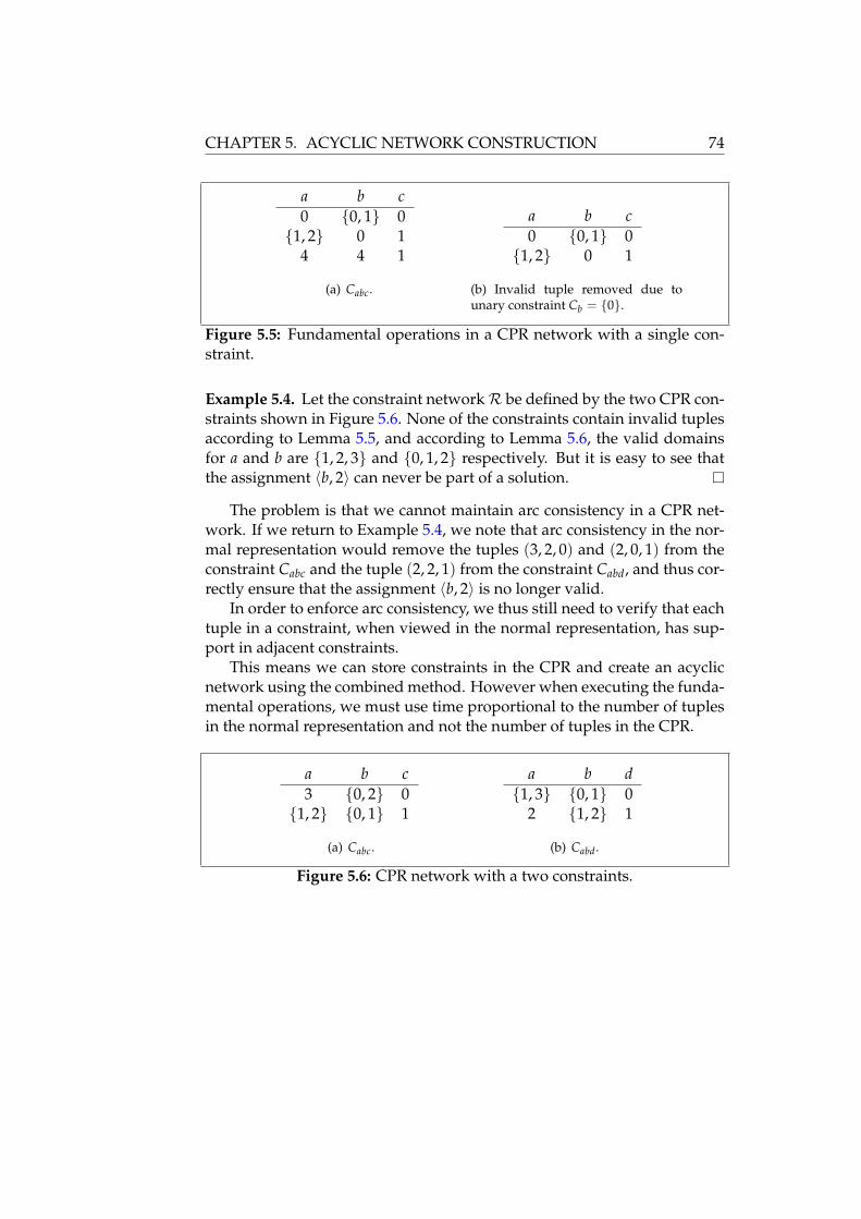
CHAPTER 5. ACYCLIC NETWORK CONSTRUCTION 74
a b c0 0, 1 01, 2 0 1
4 4 1
(a) Cabc.
a b c0 0, 1 01, 2 0 1
(b) Invalid tuple removed due tounary constraint Cb = 0.
Figure 5.5: Fundamental operations in a CPR network with a single con-straint.
Example 5.4. Let the constraint networkR be defined by the two CPR con-straints shown in Figure 5.6. None of the constraints contain invalid tuplesaccording to Lemma 5.5, and according to Lemma 5.6, the valid domainsfor a and b are 1, 2, 3 and 0, 1, 2 respectively. But it is easy to see thatthe assignment 〈b, 2〉 can never be part of a solution.
The problem is that we cannot maintain arc consistency in a CPR net-work. If we return to Example 5.4, we note that arc consistency in the nor-mal representation would remove the tuples (3, 2, 0) and (2, 0, 1) from theconstraint Cabc and the tuple (2, 2, 1) from the constraint Cabd, and thus cor-rectly ensure that the assignment 〈b, 2〉 is no longer valid.
In order to enforce arc consistency, we thus still need to verify that eachtuple in a constraint, when viewed in the normal representation, has sup-port in adjacent constraints.
This means we can store constraints in the CPR and create an acyclicnetwork using the combined method. However when executing the funda-mental operations, we must use time proportional to the number of tuplesin the normal representation and not the number of tuples in the CPR.
a b c3 0, 2 01, 2 0, 1 1
(a) Cabc.
a b d1, 3 0, 1 0
2 1, 2 1
(b) Cabd.
Figure 5.6: CPR network with a two constraints.

CHAPTER 6
Performance Study
The algorithms for the fundamental operations described in Chapter 4 andthe methods for acyclic network construction described in Chapter 5 havebeen implemented and the performance has been tested on various prob-lem instances. This chapter contains a brief description of the implemen-tation and the problem instances used, as well as the result of the perfor-mance study.
6.1 Implementation
The methods for acyclic network construction described in Sections 5.3 and5.1, as well as algorithms for the fundamental operations described in Sec-tion 4.5 on page 47, have been implemented and this section contains abrief overview of the implementation. The complete source (comprisingapproximately 7000 lines of non-comment C++ code in 40 files) is availableelectronically. See Appendix A on page 109 for details on how to obtainand compile the code as well as a brief description of the source files.
Preprocessing
For many practical applications, preprocessing techniques can reduce thesize of the combinatorial problem significantly. As an example, Weihe[1998] reported that preprocessing completely solved many instances ofa problem, equivalent to the NP-complete hitting set problem [Garey andJohnson, 1979], arising from the German and European train schedules.The problems not solved by preprocessing were easily solved by hand.
Two preprocessing rules were applied to the constraint networks usedin this performance study:
75

CHAPTER 6. PERFORMANCE STUDY 76
1. Repeatedly replace two constraints that have the same scope with thesingle constraint obtained by joining the two constraints.
2. Repeatedly replace two constraints, where the scope of one constraintis a subset of the other, with the single constraint obtained by joiningthe two constraints.
If constraints are not in the CPR form, these rules will always decreasethe total size of the constraint network since the size of the joined resultwill never be larger than any of the two relations. For constraints in theCPR form, however, this may not be the case since the joined result may belarger than any of the two relations.
For some networks these rules have no effect, but for many of the net-works arising from practical applications the effect can be dramatic as thefollowing example shows.
Example 6.1. The “car” instance (see Section 6.2 on page 81 for more de-tails) contains 7883 constraints and has size 2071515. Applying the first re-duction rule took 11 CPU seconds and resulted in a network with 849 con-straints and size 593403. Applying the second rule took 54 CPU secondsand resulted in a network with 199 constraints and size 697216. Withoutpreprocessing, none of the methods for acyclic network construction wereable to complete the compilation.
Array-Based Logic
The implementation of array-based logic is straightforward. All constraintsare compressed and we select a pair of constraints to be joined based onthe connectivity factor (cf., Equation (5.6) on page 62). The joined result iscompressed and we select the next pair of constraints to be joined. Whenthere is a single constraint left, we are finished.
Tree Clustering
The implementation of the tree clustering method is based on the algo-rithms described by Tsang [1993]. Triangulation of the primal graph isdone using a naive algorithm having O(n2) worst-case running time. Inall the instances used in the performance study, this turned out not to be aproblem since triangulation was performed in a few seconds.
Tsang [1993] notes that the triangulation heuristic can be used with anarbitrary node ordering, and suggests the use of the maximum cardinal-ity ordering which has the nice property that no edges are added if thegraph is already chordal. The nodes are ordered by first selecting an arbi-trary node and then repeatedly selecting the unordered node adjacent tothe maximum number of already ordered nodes. However, El Fattah and

6.1. IMPLEMENTATION 77
Dechter [1996] observed a dramatic difference in the effects of various or-dering heuristics on the resulting join tree obtained from the tree clusteringmethod. In all the instances tested, they found that the minimum degreeordering produced the smallest cliques.
The minimum degree ordering is computed from last to first by repeat-edly selecting the node having the least number of neighbors in the graph(hence minimum degree). When a node has been selected, the node andthe incident edges are removed from the graph and the neighbors of theremoved nodes are connected. The process is continued until the graph isempty.
George and Liu [1989] give a historical survey of the minimum degreeordering and the improvements made to the basic algorithms. We use theminimum degree ordering implementation provided by the Boost Graph Li-brary1 [Siek et al., 2001].
6.1.1 Correctness
It is difficult to determine if an implementation always computes the cor-rect results. Basically, there are two ways to determine this:
1. Formally prove that the implementation correctly implements the al-gorithms required. If the algorithms are proved correct, this ensuresthe correctness of the implementation.
This is usually not feasible for programs of any significant size and iseven more difficult when the implementation language is C++ whereside effects and pointer aliasing can occur.
2. Construct an exhaustive list of test instances and manually verify thatthe correct results are produced.
Constructing the test instances such that all possible combinations ofcode paths are tested is very time consuming and difficult withoutautomated tools for testing code coverage.
A pragmatic solution has been chosen to at least ensure some valid-ity of the implementation. It is asserted, that the major steps in the meth-ods compute the correct results (i.e., that the triangulation algorithm in factcomputes a triangulation). All the acyclic networks constructed have beentested against a commercial CSP solver2 on the belief that this solver hasreceived thorough testing and use by various customers. It is verified thatthe addition of every possible unary constraint has the same effect in bothimplementations.
1The version used was 1.29, available at www.boost.org .2Array Database v5.5 by Array Technology A/S, www.arraytechnology.com .

CHAPTER 6. PERFORMANCE STUDY 78
6.1.2 Implementation Details
The basic algorithm for compressing constraints is based on that presentedin [Katajainen and Madsen, 2002]. The basic algorithm for joining con-straints is based on the implementation presented in [Madsen, 2002] butmodified according to the suggestions in [Madsen, 2002, p. 29] so that theamount of memory required is proportional to the size of the output.
Data structures
There are basically two ways to layout a relation in memory:
Horizontally decomposed: The values of each tuple form a consecutivebyte sequence.
Vertically decomposed: The values of each column form a consecutive bytesequence.
When joining two relations, we need to compare values for the columnscommon to both relations. This is usually not all the values in a tuple,so the stride, i.e., the offset between two subsequently accessed memoryaddresses, will be larger than one. In [Boncz et al., 2000], experiments showthat the stride size is an important parameter for optimizing memory accesspatterns in join algorithms. On a simple in-memory scan of a single bytefrom 200000 tuples, an increase of a factor of 8 was measured in executiontimes when the stride was increased from 1 to 150 bytes.
We therefore choose the vertical decomposition since values of a singlecolumn can then be accessed sequentially. This choice has another benefit:the tuple width need not be uniform. This means that values in a com-pressed column can vary in size.
A consequence of this choice is that all algorithms should preferablywork column-wise instead of tuple-wise in order to maximize the localityof memory access.
Representing columns
As noted earlier, each column in a relation contains values from a finitedomain Dx. Without loss of generality, we therefore encode the domainvalues as integers 0, 1, . . . , |Dx| − 1.
There are several ways to represent the sets in a compressed column ofa CPR relation. We need to be able to efficiently determine
• whether the intersection between two sets is empty,
• the intersection between two sets, and
• whether a given element exists in a set.

6.1. IMPLEMENTATION 79
For small domains, a bit vector seems like a natural choice: the intersectionoperation can utilize the inherent word-parallelism of the bitwise AND op-erator and the single element test is simply a bit test. But for large domains,the memory usage of the bit vector becomes prohibitive since we assumethe sets are sparse. The methods for representing a column are therefore asfollows:
Uncompressed columns: Stored as a sequence of integers. The number ofbits needed for each integer is dlog2 |Dx|e, |Dx| ≥ 1. To minimize thememory usage, we represent an integer as the smallest native datatype that can hold dlog2 |Dx|e bits. In the current implementation thisis either 8, 16, or 32 bits.
Compressed columns: Stored as a sequence of either fixed-sized bit vec-tors or (pointers to) sorted integer vectors.
In the current implementation, bit vectors are used when the domainhas no more than 28 = 256 values. This enables encoding the set in at most8 32-bit words. It is likely that it is beneficial to encode even larger domainsas bit vectors, since we avoid memory allocation for set elements and weexhibit better cache behavior. The exact size where the encoding shouldswitch to using a sorted vector, should be determined experimentally.
Using optimal representations
The columns are represented using different classes depending on whethera column is compressed and on the domain size of the corresponding vari-able. The creation of the optimal class for any given variable is imple-mented in a central factory function, which creates new columns. For com-pressed columns, it looks as follows.CompressedColumn ∗CompressedColumn : : createNew ( Var iab le & var ,
s i z e _ t rowCount )s i z e _ t max_dom_index = var . getDomainSize ( ) −1;
i f ( max_dom_index < 8 )return new BitmapCompressedColumn <8>( var , rowCount ) ;
i f ( max_dom_index < 1 6 )return new BitmapCompressedColumn <16 >( var , rowCount ) ;. . .
i f ( max_dom_index < 2 5 6 )return new BitmapCompressedColumn <256 >( var , rowCount ) ;
i f ( max_dom_index ≤ std : : numeric_l imits <unsigned char > : : max ( ) )return new ConcreteCompressedColumn<unsigned char >( var ,
rowCount ) ;i f ( max_dom_index ≤ std : : numeric_l imits <unsigned short > : : max ( ) )
return new ConcreteCompressedColumn<unsigned short >( var ,rowCount ) ;
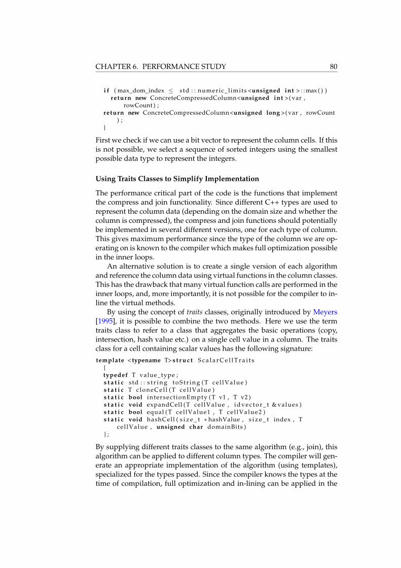
CHAPTER 6. PERFORMANCE STUDY 80
i f ( max_dom_index ≤ std : : numeric_l imits <unsigned int > : : max ( ) )return new ConcreteCompressedColumn<unsigned int >( var ,
rowCount ) ;return new ConcreteCompressedColumn<unsigned long >( var , rowCount
) ;
First we check if we can use a bit vector to represent the column cells. If thisis not possible, we select a sequence of sorted integers using the smallestpossible data type to represent the integers.
Using Traits Classes to Simplify Implementation
The performance critical part of the code is the functions that implementthe compress and join functionality. Since different C++ types are used torepresent the column data (depending on the domain size and whether thecolumn is compressed), the compress and join functions should potentiallybe implemented in several different versions, one for each type of column.This gives maximum performance since the type of the column we are op-erating on is known to the compiler which makes full optimization possiblein the inner loops.
An alternative solution is to create a single version of each algorithmand reference the column data using virtual functions in the column classes.This has the drawback that many virtual function calls are performed in theinner loops, and, more importantly, it is not possible for the compiler to in-line the virtual methods.
By using the concept of traits classes, originally introduced by Meyers[1995], it is possible to combine the two methods. Here we use the termtraits class to refer to a class that aggregates the basic operations (copy,intersection, hash value etc.) on a single cell value in a column. The traitsclass for a cell containing scalar values has the following signature:template < typename T> s t r u c t S c a l a r C e l l T r a i t s
typedef T value_type ;s t a t i c std : : s t r i n g t o S t r i n g ( T c e l l V a l u e )s t a t i c T c l o n e C e l l ( T c e l l V a l u e )s t a t i c bool in tersect ionEmpty ( T v1 , T v2 )s t a t i c void expandCell ( T ce l lValue , i d v e c t o r _ t & values )s t a t i c bool equal ( T ce l lValue1 , T c e l l V a l u e 2 )s t a t i c void hashCell ( s i z e _ t ∗ hashValue , s i z e _ t index , T
ce l lValue , unsigned char domainBits ) ;
By supplying different traits classes to the same algorithm (e.g., join), thisalgorithm can be applied to different column types. The compiler will gen-erate an appropriate implementation of the algorithm (using templates),specialized for the types passed. Since the compiler knows the types at thetime of compilation, full optimization and in-lining can be applied in the

6.2. PROBLEM INSTANCES 81
critical inner loops. In this case, virtual functions are only used to call thecorrect (compiler generated) function. We have such created a bridge be-tween the generic programming paradigm and the object oriented programmingparadigm.
6.2 Problem Instances
The problem instances used in the performance study fall in various cate-gories. The most interesting category is the configuration problems as theseare the problems that require interactivity. The remaining categories are in-cluded to see how well the compilation methods perform with other typesof networks.
In the following, a number of problem instances, which have been col-lected from various sources, are described. For all instances, n denotes thenumber of variables, e the number of constraints, r the largest arity of aconstraint, d the size of the largest domain, |Dx| the size of the domain forvariable x, ‖R‖ the size of the network, t the largest number of tuples in aconstraint, |κ(R)| the size of the network in compressed form, and finallytκ the largest number of tuples in a compressed constraint.
The symbol † is used to represent a number larger than 1.7 × 10308,which is the maximal value representable in an 8 byte floating-point num-ber.
Configuration Problems
The instances presented in Table 6.1 on page 83 are networks which orig-inate from real life configuration problems. The “renault” instance is thetest problem described in [Amilhastre et al., 2002] and deals with configu-ration of a specific family of cars called Renault Megane3. The remaininginstances have been provided by Array Technology A/S and have beencollected during various customer projects. The constraint graphs for theinstance “ns11” are depicted in Figure 6.1 on the following page.
Circuit Verification
The ISCAS ’85 benchmark suite consists of a logical description of 10 elec-tronic circuits, provided to authors at the 1985 International Symposium onCircuits and Systems [Brglez and Fujiwara, 1985]. They have subsequentlybeen used by many researchers as a basis for comparing results in the area
3At the time of writing, the problem instance was available at ftp://ftp.irit.fr/pub/IRIT/RPDMP/Configuration/ .

CHAPTER 6. PERFORMANCE STUDY 82
(a) Primal constraint graph.
(b) Dual constraint graph.
Figure 6.1: Constraint graphs for instance ns11.

6.2. PROBLEM INSTANCES 83
Name n e r d Πx∈X |Dx| ‖R‖ t ‖κ(R)‖ tκ
renault 101 113 10 42 6.84× 1049 1.29× 10⁶ 4.87× 10⁴ 29279 104plan-2-25 417 290 16 3 2.32× 10147 1.51× 10⁵ 2.05× 10³ 10787 192plan-31 283 394 30 3 2.30× 1088 2.38× 10¹² 1.56× 10¹⁰ 62803 118
car 184 7879 17 42 1.58× 1082 1.35× 10¹⁶ 3.95× 10¹² 2071511 17shelf 50 43 3 132 3.12× 1076 1.85× 10⁵ 5.15× 10³ 155850 5151cf0-td 29 310 7 118 3.70× 10²⁰ 4.64× 10⁷ 8.04× 10⁵ 41123 6heq 1157 586 6 4 † 5.74× 10⁴ 9.00× 101 23709 16ns11 77 74 11 8 4.25× 1053 8.19× 10⁸ 1.24× 10⁷ 34403 296
Table 6.1: Characteristics of configuration problem instances.
of test generation and circuit verification. Each circuit4 is described in Ta-ble 6.2.
From each circuit a constraint network is created. There is a Booleanvariable for each gate’s output and for all the circuit inputs. For each con-nection in the circuit a corresponding constraint is created which maintainsthe relations between a gate’s input and output. The characteristics of theresulting networks are presented in Table 6.3 on page 85. While these prob-lems do not require interactivity, they are included here to see how thecompilation methods behave on structured constraint networks. The con-straint graphs for the instance “c432” are depicted in Figure 6.2 on the nextpage.
Circuit Circuit Total Input OutputName Function Gates Lines Lines
c432 Priority Decoder 160 (18 EXOR) 36 7c499 ECAT 202 (104 EXOR) 41 32c880 ALU and Control 383 60 26c1355 ECAT 546 41 32c1908 ECAT 880 33 25c2670 ALU and Control 1193 233 140c3540 ALU and Control 1669 50 22c5315 ALU and Selector 2307 178 123c6288 16-bit Multiplier 2406 32 32c7552 ALU and Control 3512 207 108
Table 6.2: ISCAS ’85 benchmark circuits.
4At the time of writing, the net-lists for the circuits were available at http://www.cbl.ncsu.edu/www/CBL_Docs/iscas85.html .

CHAPTER 6. PERFORMANCE STUDY 84
(a) Primal constraint graph.
(b) Dual constraint graph.
Figure 6.2: Constraint graphs for circuit c432.

6.2. PROBLEM INSTANCES 85
Name n e r d Πx∈X |Dx| ‖R‖ t ‖κ(R)‖ tκ
c432 196 160 10 2 1.00× 1059 2.02× 10⁴ 5.12× 10² 2176 10c499 243 202 6 2 1.41× 1073 4.22× 10³ 3.20× 101 2486 6c880 443 383 5 2 2.27× 10133 5.29× 10³ 1.60× 101 3803 5
c1355 587 546 6 2 5.07× 10176 8.10× 10³ 3.20× 101 5526 6c1908 913 880 9 2 6.92× 10274 2.85× 10⁴ 2.56× 10² 8389 9c2670 1426 1193 6 2 † 1.63× 10⁴ 3.20× 101 10865 6c3540 1719 1669 9 2 † 5.61× 10⁴ 2.56× 10² 16012 9c5315 2485 2307 10 2 † 4.86× 10⁴ 5.12× 10² 24267 10c6288 2448 2416 3 2 † 2.87× 10⁴ 4.00× 1000 23968 3c7552 3719 3512 6 2 † 5.09× 10⁴ 3.20× 101 32228 6
Table 6.3: Characteristics of circuit verification problem instances.
Satisfiability Problems
The instances presented in Table 6.4 are networks which originate fromsatisfiability benchmarks. All the networks presented are instances of thepigeon hole problem. We are asked whether it is possible to place h + 1 pi-geons in h holes such that no hole contains more than one pigeon. This isclearly an unsatisfiable problem.
The encoding of this problem is straightforward5. For each pigeon iwe have a variable xij which means that pigeon i is placed in hole j. Thenwe have h + 1 clauses which say that a pigeon has to be placed in somehole. For each hole we have a set of clauses ensuring that only a singlepigeon is placed into that hole. This encoding leads to a total of h(h + 1)Boolean variables and (h + 1) + h(h(h + 1)/2) constraints. As can be seenin Figure 6.3 on the next page, both the primal and dual constraint graphsare highly symmetric, which makes graph-based decomposition difficult.
Name n e r d Πx∈X |Dx| ‖R‖ t ‖κ(R)‖ tκ
hole6 42 133 6 2 4.40× 10¹² 3.40× 10³ 6.30× 101 987 6hole7 56 204 7 2 7.21× 10¹⁶ 8.29× 10³ 1.27× 10² 1540 7hole8 72 297 8 2 4.72× 10²¹ 2.01× 10⁴ 2.55× 10² 2268 8hole9 90 415 9 2 1.24× 1027 4.84× 10⁴ 5.11× 10² 3195 9hole10 110 561 10 2 1.30× 1033 1.16× 10⁵ 1.02× 10³ 4345 10
Table 6.4: Characteristics of satisfiability problem instances.
5At the time of writing, CNF instances were available at http://www.intellektik.informatik.tu-darmstadt.de/SATLIB/benchm.html .

CHAPTER 6. PERFORMANCE STUDY 86
(a) Primal constraint graph. (b) Dual constraint graph.
Figure 6.3: Constraint graphs for the pigeon hole problem for h = 6.
Puzzles
The instances presented in Table 6.5 are all instances of the n-queen prob-lem for various values of n. The formulation used is similar to that of Ex-ample 3.1 on page 20. While the n-queens problem is a popular benchmark,it has very specific features unlikely for to be found in real-life problems.First, all constraints are binary. Second, every variable is constrained byevery other variable. This makes graph based decomposition difficult asboth the primal and dual constraint graph are completely symmetric. Anexample for n = 8 is shown in Figure 6.4 on the facing page.
Name n e r d Πx∈X |Dx| ‖R‖ t ‖κ(R)‖ tκ
queens8 8 28 2 8 1.68× 10⁷ 2.58× 10³ 5.40× 101 1302 8queens9 9 36 2 9 3.87× 10⁸ 4.37× 10³ 7.00× 101 2193 9
queens10 10 45 2 10 1.00× 10¹⁰ 6.96× 10³ 8.80× 101 3394 10queens11 11 55 2 11 2.85× 10¹¹ 1.06× 10⁴ 1.08× 10² 5111 11queens12 12 66 2 12 8.92× 10¹² 1.54× 10⁴ 1.30× 10² 7372 12
Table 6.5: Characteristics of puzzle problem instances.

6.3. EXPERIMENTAL PROTOCOL 87
(a) Primal constraint graph. (b) Dual constraint graph.
Figure 6.4: Constraint graphs for the 8-queen problem.
6.3 Experimental Protocol
Two metrics are interesting when trying to asses the practical value of themethods described in the preceding sections:
1. The time it takes to construct an acyclic network for a given probleminstance.
2. The worst-case and average-case time it takes to execute one of thethree fundamental operations described in Section 4.3 on page 42.
The first metric is obtained by compiling the instances presented in Sec-tion 6.2. For each instance, the running time (measured in number of CPUseconds in user mode) and the memory usage (measured in megabytes) arereported. A limit of 2 CPU hours and 512MB memory has been set on therunning time and memory usage respectively.
For the second metric, I use the method introduced in [Amilhastre et al.,2002], where we “simulate” the behavior of a user interacting with the con-straint solver:
1. Process the variables according to some random ordering.
2. If the number of valid domain values for the variable being processedis 1, continue with the next variable.
3. Order the valid domain values for the variable being processed. CallADD-CONSTRAINT with the selected variable and domain value.

CHAPTER 6. PERFORMANCE STUDY 88
4. Report the CPU time used in the call to ADD-CONSTRAINT.
The simulation is complete when all variables have a single valid domainvalue. For each instance, 20, 000 simulations are performed and the cu-mulative distribution function of the measured time is reported as well asthe average and worst-case time. We restrict the simulation to test ADD-CONSTRAINT, since the performance of the other fundamental operationsshould be proportional.
All experiments were carried out on a Dell Inspiron 8200 Laptop witha Pentium 4-M 2GHz CPU, 512MB memory, and running Windows XP.All code has been compiled with Microsoft Visual C++ 7.0 using the -O2optimization flag.
6.4 Experimental Results
The compilation results obtained using array-based logic are shown in Ta-ble 6.6 on the facing page. The symbol 3 in one of the columns ’CPU’or ’Mem’ indicates that the compilation process could not be completedwithin the given limits for that column. If the compilation succeeded, thecharacteristics of the resulting acyclic network is reported. Note that forarray-based logic, the acyclic network always contains a single n-ary rela-tion.
The compilation results obtained using the tree clustering method areshown in Table 6.7 on page 90. For the tree clustering method, the over-all complexity is dependent on the size of the largest clique found in thedecomposition phase. This is reported as r, the arity of the largest scope,in the acyclic network. Similarly, the number of cliques is reported as e,the number of constraints in the acyclic network. Note that the size of thecliques found for the circuit verification instances differ from the numbersreported by El Fattah and Dechter [1996]. This is in all likelihood attributedto the use of a different implementation of the minimum degree orderingheuristic.
Simulation Results
The running time of ADD-CONSTRAINT depends quadratically on the num-ber of uncompressed tuples in the acyclic network. The simulations havetherefore been restricted to the configuration problem instances where themaximum number of uncompressed tuples is small. The remaining in-stances all required running times in excess of 1 hour, clearly not feasiblefor interactive use. The results of the simulations are shown in Table 6.8 onpage 90. The percentages shown in the table are the cumulative distribu-tion function of the running times, i.e., for the “car” instance 8% of the callscompleted within 0.01 seconds and 87% completed within 0.05 seconds.

6.5. DISCUSSION OF RESULTS 89
Name CPU Mem ‖R‖ t ‖κ(R)‖ tκ
renault 3
plan-2-25 3
plan-31 3
car 3
shelf 3
cf0-td 44.6 229 5.98× 10¹⁴ 2.14× 10¹³ 19625700 135792heq 3
ns11 3
c432 3
c499 3
c880 3
c1355 3
c1908 3
c2670 3
c3540 3
c5315 3
c6288 3
c7552 3
hole6 2.1 44hole7 394.4 70hole8 3
hole9 3
hole10 3
queens8 0.23 14 7.36× 10² 9.20× 101 736 92queens9 1.9 46 3.17× 10³ 3.52× 10² 3168 352queens10 178.2 75 7.24× 10³ 7.24× 10² 7240 724queens11 5546 248 2.95× 10⁴ 2.68× 10³ 29480 2680queens12 3
Table 6.6: Compilation results using array-based logic.
The table shows that most calls complete within a few seconds but forthe “renault” instance some calls take more than 6 seconds, barely tolerablefor interactive use. This pattern is caused by the fact that , initially, manycombinations are valid but as soon as a constraint is added, the numberof valid combinations is reduced and the subsequent calls thus require lesstime to execute.
6.5 Discussion of Results
If we look at the characteristics of the different problem instances, we seethat using the CPR for constraints is beneficial, especially for the configu-ration problems where the domain sizes are large. The extreme case is the

CHAPTER 6. PERFORMANCE STUDY 90
Name CPU Mem e r ‖R‖ t ‖κ(R)‖ tκ
renault 12.4 10 84 10 1.30× 10⁶ 2.83× 10⁴ 57222 328plan-2-25 6.3 8 289 23 6.30× 10⁸ 1.03× 10⁷ 128718 1560plan-31 265.3 130 98 44 7.80× 10¹⁴ 8.80× 10¹² 251879 478
car 180.4 82 166 16 3.99× 10⁵ 1.46× 10⁴ 22458 65shelf 1.8 5 39 6 8.15× 10⁹ 2.55× 10⁸ 147243 710cf0-td 9.2 22 21 9 1.31× 10⁹ 1.01× 10⁸ 239909 897heq 4.1 7 643 10 3.88× 10⁵ 2.59× 10³ 44157 40ns11 16.7 13 40 14 4.56× 10⁸ 1.92× 10⁷ 442034 9265
c432 2.2 5 157 28 1.88× 10⁹ 3.41× 10⁷ 10949 36c499 2.6 5 195 25 2.00× 10⁹ 3.77× 10⁷ 11150 144c880 3.6 6 357 26 1.86× 10⁹ 3.36× 10⁷ 11547 18
c1355 4.7 7 435 25 2.01× 10⁹ 3.77× 10⁷ 15078 144c1908 58.7 33 719 56 1.96× 10¹⁷ 2.53× 10¹⁵ 965458 5340c2670 17.8 16 1168 38 2.66× 10¹² 6.87× 10¹⁰ 37000 36c3540 166.6 69 1442 122 5.36× 1036 4.15× 1034 196139 384c5315 105.5 48 2050 74 6.12× 10²¹ 7.38× 10¹⁹ 173791 256c6288 133.4 58 1980 59 1.47× 10¹⁹ 1.37× 10¹⁷ 347392 1600c7552 160.8 45 3036 47 1.40× 10¹⁵ 1.95× 10¹³ 203911 256
hole6 33 12 11 28 2.55× 10⁶ 5.15× 10⁴ 400179 10000hole7 35.6 133 13 36 2.48× 10⁸ 4.67× 10⁶ 5114711 82944hole8 3 15 46hole9 3 17 58hole10 3 19 72
queens8 0.51 45 1 8 7.36× 10² 9.20× 101 736 92queens9 2.3 46 1 9 3.17× 10³ 3.52× 10² 3168 352
queens10 18.5 49 1 10 7.24× 10³ 7.24× 10² 7240 724queens11 3 1 11queens12 3 1 12
Table 6.7: Compilation results using the tree clustering method.
%(CPU time ≤ X)Name 0.001 0.005 0.01 0.05 0.1 5.0 10.0 Avg Max
renault 0% 54% 73% 85% 88% 97% 100% 0.24 6.31car 0% 0% 8% 87% 89% 100% 100% 0.06 1.09heq 0% 0% 0% 0% 0% 100% 100% 0.11 0.19
Table 6.8: Results of running simulations of ADD-CONSTRAINT.
6.5. DISCUSSION OF RESULTS 91
“car” instance where the maximum number of tuples is decreased from3.95× 1012 to just 17.
The compilation results for array-based logic show, that even if the CPRis used, this method is only feasible for the smallest problems.
The compilation results for the tree clustering method show that it isfeasible to use this method to construct an acyclic constraint network. Allthe configuration problems were compiled in less than 4 minutes, and mostproblems compiled in only a few seconds.
We also note that for the n-queen instances, tree clustering does not im-prove the results. This is not surprising as the primal constraint graph iscomplete in thus only a single clique is found, i.e., the method degeneratesto array-based logic. For most real-life problems it is expected, however,that the constraint graph has a structure that enables smaller cliques to befound, as was the case with all the real-life instances used in this perfor-mance study.
Tree clustering alone is not sufficient to detect that the pigeon hole prob-lems are unsatisfiable. We need to enforce arc consistency on the acyclicnetwork to detect this.
While the CPR is applicable when constructing the acyclic network, theusefulness is not obvious when it comes to execution of the fundamentaloperations since the running time depends quadratically on the numberof tuples in the uncompressed form. This in turn means that, if we re-quire response times within a few seconds, the methods described in thepreceding sections are only applicable when the number of tuples in theuncompressed acyclic network is small.

CHAPTER 6. PERFORMANCE STUDY 92

CHAPTER 7
Uniform Acyclic Networks
The results from Chapter 6 showed that, while the algorithms for the fun-damental operations are polynomial in the size of the acyclic network, theacyclic networks constructed from most of the real-life problem instanceswere too large to solve interactively. The main reason is that the runningtime of ARC-CONSISTENCY is quadratic in the number of tuples in the un-compressed acyclic network. If we could somehow avoid working withthe uncompressed acyclic network, we would stand a much better chanceof achieving the desired response time.
In this chapter, I show how we can maintain arc consistency for con-straints in the compressed form by imposing an additional requirementon the structure of the acyclic network to get a uniform acyclic network. Aheuristic is then presented which transforms an acyclic network obtainedfrom the tree clustering method into a uniform acyclic network. The chap-ter is concluded with experimental results obtained by executing the treetransformation and running the simulation on the resulting uniform acyclicnetwork.
In the following sections, I assume that all constraint networks are usingthe CPR. All results generalize to networks in the normal representation ifeach scalar value is treated as a singleton set.
7.1 Fundamental Operations in Uniform Acyclic Net-works
It turns out that, if we restrict the acyclic network so that two constraintsshare at most a single variable, we can maintain arc consistency in the dualnetwork of an acyclic CPR network. I call this restricted acyclic network a
93
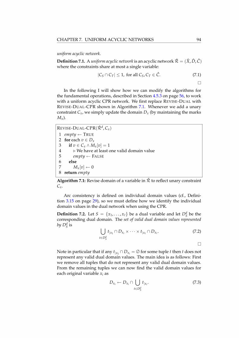
CHAPTER 7. UNIFORM ACYCLIC NETWORKS 94
uniform acyclic network.
Definition 7.1. A uniform acyclic network is an acyclic network R = (X, D, C)where the constraints share at most a single variable:
|CS ∩ CT | ≤ 1, for all CS, CT ∈ C. (7.1)
In the following I will show how we can modify the algorithms forthe fundamental operations, described in Section 4.5.3 on page 56, to workwith a uniform acyclic CPR network. We first replace REVISE-DUAL withREVISE-DUAL-CPR shown in Algorithm 7.1. Whenever we add a unaryconstraint Cx, we simply update the domain Dx (by maintaining the marksMx).
REVISE-DUAL-CPR(Rd, Cx)1 empty ← TRUE
2 for each v ∈ Dx3 if v ∈ Cx ∧Mx[v] = 14 . We have at least one valid domain value5 empty ← FALSE
6 else7 Mx[v] ← 08 return empty
Algorithm 7.1: Revise domain of a variable in R to reflect unary constraintCx.
Arc consistency is defined on individual domain values (cf., Defini-tion 3.15 on page 29), so we must define how we identify the individualdomain values in the dual network when using the CPR.
Definition 7.2. Let S = x1, . . . , x` be a dual variable and let DdS be the
corresponding dual domain. The set of valid dual domain values representedby Dd
S is ⋃t∈Dd
S
t|x1 ∩ Dxi × · · · × t|x`∩ Dx`
. (7.2)
Note in particular that if any t|x1 ∩Dxi = ∅ for some tuple t then t does notrepresent any valid dual domain values. The main idea is as follows: Firstwe remove all tuples that do not represent any valid dual domain values.From the remaining tuples we can now find the valid domain values foreach original variable xi as
Dxi ← Dxi ∩⋃
t∈DdS
t|xi. (7.3)

7.1. FUNDAMENTAL OPERATIONS 95
This is formalized in Algorithm 7.2 and we can now prove the followingtheorems.
REVISE-CPR(S, T)1 . Note T is not used, but included to maintain signature compatibility
with REVISE-20012 changed ← FALSE
3 . Mark invalid rows4 for i ← 1 to |Dd
S|5 for each x ∈ S6 if Dd
S[i]|x ∩ Dx = ∅7 Md
S[i] ← 08 . Update valid domains9 for each x ∈ S
10 M[1..|Dx|] ← 011 for i ← 1 to |Dd
S|12 if Md
S[i] = 113 for each v ∈ Dd
S[i]|x14 M[v] = 115 for j ← 1 to|Dx|16 if M[j] = 017 if Dx[j] = 118 changed ← TRUE
19 Dx[j] ← 020 return changed
Algorithm 7.2: Mark invalid tuples and update valid domain values oforiginal variables.
Theorem 7.1. Let S and T be two dual variables such that S ∩ T = x. Afterthe calls REVISE-CPR(S, T), and REVISE-CPR(T, S) S is arc consistent relativeto T and T is arc consistent relative to S, when we consider the set of valid domainvalues, as defined in Definition 7.2 on the preceding page, represented by Dd
S andDd
T.
Proof. Lines 4–7 mark the tuples that do not represent any valid domainvalues. Lines 10–14 compute the union
⋃t∈Dd
St|xi
and lines 15–19 computethe set Dxi according to Equation (7.3) on the facing page.
To prove S arc consistent with T, we must prove that for all u ∈ DdS
that represents a valid domain value and all a ∈ u|x ∩ Dx, there exists atuple v ∈ Dd
T that represents a valid domain value such that a ∈ v|x ∩ Dx.We know that a ∈ Dx. In the call to REVISE-CPR(T, S) we computed Dx

CHAPTER 7. UNIFORM ACYCLIC NETWORKS 96
according to Equation (7.3) on page 94 so we have
a ∈ Dx ⊆⋃
u∈DdT
u|x. (7.4)
That T is arc consistent with S is proved similarly.
Theorem 7.2. Let R = (X, D, C) be a uniform acyclic CPR network. Let Rd
be the corresponding dual network. If we replace REVISE-2001 with REVISE-CPR shown in Algorithm 7.2 on the preceding page, ARC-CONSISTENCY (Algo-rithm 4.6 on page 55) maintains arc consistency in Rd in worst-case timeO(redt2
κ).
Proof. We first note that for each arc S, T in the dual network, we callboth REVISE-CPR(S, T) and REVISE-CPR(T, S) in the initial loop of ARC-CONSISTENCY. Subsequently, according to Theorem 7.1, the only way S canbecome arc inconsistent relative to T is if a tuple in Dd
S becomes invalid.This can only happen if any of the domains of the original variables in Schange, however in this case S is added to Q and REVISE-CPR(T, S) willbe called and arc consistency restored. The same argument applies when Tbecomes arc inconsistent relative to S.
For the complexity result, we note that in PROPAGATION, the call toREVISE-CPR only returns FALSE when a new invalid tuple is found. Thereare at most tκ tuples in each dual variable and a total of e dual variables.The time complexity of REVISE-CPR is O(rdtκ) since we can compute theintersections in time at most O(d). This proves the result.
Replacing REVISE-2001 with REVISE-CPR essentially creates an algo-rithm resembling AC-3, though now working with CPR constraints in thedual network. Note, that, in order not to change the algorithms from Chap-ter 4, Theorem 7.2 did not utilize the fact that the dual network is a tree.In the case where we call ADD-CONSTRAINT on a original variable x, wecan apply REVISE-CPR from root nodes to leaf nodes and back, in the treerooted at some dual variable containing x. In this case we can achieve arc-consistency in worst-case time O(redtκ).
7.1.1 Summary of Results
REVISE-CPR updates the domains of the original variables, so we no longerneed VALID-DOMAINS. By making the changes proposed in the preced-ing section, we can thus execute the fundamental operations in a uniformacyclic network containing CPR constraints. The complexity results aresummarized in Table 7.1 on the next page.

7.2. UNIFORM ACYCLIC NETWORK CONSTRUCTION 97
Function Time Complexity Space Complexity
ADD-CONSTRAINT O(redt2κ) O(etκ)
REMOVE-CONSTRAINT O(redt2κ) O(etκ)
RESTORATION O(|H|redt2κ) O(etκ)
Table 7.1: Complexity results for the fundamental operations in a uniformacyclic network.
7.2 Uniform Acyclic Network Construction
A uniform acyclic network can be constructed by a tree transformation thattransforms the tree generated by the tree clustering method into a uniformacyclic network.
A new relational operation called split forms the basis of the transfor-mation. When a constraint is split, we augment the constraint with a newmeta variable which, for each tuple, has the same valid value as the tuple’sindex. The split relation is then the projection of this meta variable on agiven set of variables.
Definition 7.3. Let S be a relation with scheme Y, Z ⊂ Y be a set of at-tributes, and let λ /∈ Y be a meta attribute. The split of S on (Z, λ), denotedτZ,λ(S) is a relation with scheme Z ∪ λ and instance
t[i]|Z × i | t[i] ∈ S, 1 ≤ i ≤ |S|. (7.5)
The split operation can be carried out in timeO(|S|). Note that for a relationS with scheme Y, a set of attributes Z ⊂ Y, we have by definition
S = πY(τZ,λ(S) 1 τY−Z,λ(S)). (7.6)
The effect of the split operator is illustrated in Figure 7.1 on the followingpage. It is easy to see that if we join the two split relations, we will get theoriginal relation from Figure 7.1(a).
The following lemma shows that we can replace a constraint by twonew constraints obtained by splitting the original constraint.
Lemma 7.3. LetR = (X, D, C) be a constraint network and CS ∈ C a constraint.Let T ⊂ S be a set of variables, and let λ be a meta variable. Furthermore, letRλ = (Xλ, Dλ, Cλ) where
Xλ = X ∪ λ (7.7)
Dλ(x) =
D(x) if x ∈ X0, . . . , |CS| − 1 if x = λ
(7.8)
Cλ = C− CS ∪ τT,λ(CS) ∪ τS−T,λ(CS). (7.9)

CHAPTER 7. UNIFORM ACYCLIC NETWORKS 98
a b c0 0 00 0 10 1 11 0 11 1 1
(a) Relation in the normal representation.
a λ
0 00 10 21 31 4
(b) τa,λ.
b c λ
0 0 00 1 11 1 20 1 31 1 4
(c) τb,c,λ.
Figure 7.1: Splitting the relation in Figure 7.1(a).
Then Sol(R) = πX(Sol(Rλ)).
Proof. Follows from Equation (7.6) on the page before.
At first it would seem that splitting a relation only increases the size of anetwork, however if we are using the CPR, we can usually reduce the totalsize, as illustrated in Figure 7.2 on the facing page, since removing variablesfrom a constraint may allow further compression. We also note that, whena constraint is split, the two new constraints are linked by a single variableas required in a uniform acyclic network.
For any constraint CS and set of variables Z ⊂ S, if we replace the con-straint CS with two new constraints τZ,λ(CS) and τS−Z,λ(CS), the meta vari-able λ represents a subset of valid tuples in the original constraint CS.
Example 7.1. If we look at Figure 7.2 on the next page, we see that the as-signment 〈λ, 3〉 in the two split constraints in Figure 7.2(e) and Figure 7.2(f)is equivalent to the following set of assignments in the original constraint:
a b c d1 1 1 01 1 1 1
Let S1, . . . , Se be a width 1 ordering of the dual variables of an acyclicnetwork (i.e., an ordering obtained by a breadth-first search in the treerooted at an arbitrary dual variable). For any dual variable Si and its parentSj, let Tij = Si− Sj. By definition, (cf., Definition 5.6 on page 67) the originalvariables in Tij are contained only in the dual variable Si and its children,not in Sj or any other dual variable at higher levels in the tree. If Tij 6= ∅it is therefore possible to split the constraint CSi and replace the originalvariables Tij in CSi with a single meta variable that represents the subsetof valid tuples for Tij. The benefits are twofold: We potentially reduce thesize of CSi and the two new relations are linked by a single meta variableas required in a uniform acyclic network.

7.2. UNIFORM ACYCLIC NETWORK CONSTRUCTION 99
a b c d0 0 0 10 0 1 00 0 1 11 1 0 11 1 1 01 1 1 1
(a) Uncompressed relation.
a b c d0 0 0 10 0 1 0, 11 1 0 11 1 1 0, 1
(b) Relation in CPR.
a b λ
0 0 00 0 11 1 21 1 3
(c) τa,b,λ.
c d λ
0 1 01 0, 1 10 1 21 0, 1 3
(d) τc,d,λ.
a b λ
0 0 0, 11 1 2, 3
(e) τa,b,λ in CPR.
c d λ
0 1 0, 21 0, 1 1, 3
(f) τc,d,λ in CPR.
Figure 7.2: Splitting a relation stored in the CPR. Note that the size of therelation in (a) is 24, (b) is 18, (c) and (d) combined is 26, and (e) and (f)combined is 17.
If the new constraint containing Tij shares more than 1 variable with itschildren, they must be joined to a single constraint. But this join operationis “local” in the sense that the resulting constraint does not influence thesize of any constraint which we need to process afterwards.
We can apply the preceding ideas to construct a uniform acyclic net-work that correctly propagates information. By processing the edges ofthe join tree in a bottom up fashion, we know that, whenever we processan edge Si, Sj, where Si is the child and Sj the parent node, the subtreerooted at Si is a uniform acyclic network. This is formalized in the algo-rithm UNIFORM-NETWORK shown in Algorithm 7.3 on the next page.
In line 7 we test if the child constraint CL contains variables that can besplit. If this is the case, lines 8-10 split the child node and add the “local”part to C and create a new constraint CS which is the join of the parentconstraint CP and the non-local part of the child constraint. If we cannotsplit the child constraint, line 12–13 simply join the child with the parent toget the constraint CS.
We now check if we can split CS. If CS does not share any variables
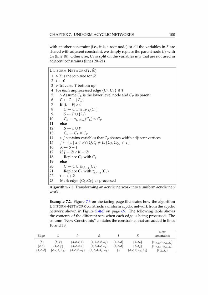
CHAPTER 7. UNIFORM ACYCLIC NETWORKS 100
with another constraint (i.e., it is a root node) or all the variables in S areshared with adjacent constraint, we simply replace the parent node CP withCS (line 18). Otherwise, CS is split on the variables in S that are not used inadjacent constraints (lines 20–21).
UNIFORM-NETWORK(T, R)1 . T is the join tree for R2 i ← 03 . Traverse T bottom up4 for each unprocessed edge CL, CP ∈ T5 . Assume CL is the lower level node and CP its parent6 C ← C− CL7 if |L− P| > 08 C ← C ∪ τL−P,λi(CL)9 S ← P ∪ λi
10 CS ← τL∩P,λi(CL) 1 CP11 else12 S ← L ∪ P13 CS ← CL 1 CP14 . J contains variables that CP shares width adjacent vertices15 J ← x | x ∈ P ∩Q, Q 6= L, CP, CQ ∈ T16 K ← S− J17 if J = ∅ ∨ K = ∅18 Replace CP with CS19 else20 C ← C ∪ τK,λi+1(CS)21 Replace CP with τJ,λi+1(CS)22 i ← i + 223 Mark edge CL, CP as processed
Algorithm 7.3: Transforming an acyclic network into a uniform acyclic net-work.
Example 7.2. Figure 7.3 on the facing page illustrates how the algorithmUNIFORM-NETWORK constructs a uniform acyclic network from the acyclicnetwork shown in Figure 5.4(e) on page 69. The following table showsthe contents of the different sets when each edge is being processed. Thecolumn “New Constraints” contains the constraints that are added in lines10 and 18.
NewEdge L P S J K constraints
b b, g a, b, c, d a, b, c, d, λ0 a, c, d b, λ0 Cg,λ0 , Cb,λ0,λ1
a, e a, e, f a, c, d, e a, c, d, e, λ2 a, c, d e, λ2 C f ,λ2, Ce,λ2,λ3
a, c, d a, c, d, λ3 a, c, d, λ1 a, c, d, λ3, λ4 a, c, d, λ3, λ4 Cλ3,λ4

7.2. UNIFORM ACYCLIC NETWORK CONSTRUCTION 101
a, e, f
a, b, c, d
a, c, d, e
b, g
(a) Initial acyclic network.
a, e, f
a, c, d, λ1
a, c, d, e
g, λ0
b, λ0, λ1
(b) After edge b has been processed.
f , λ2
a, c, d, λ1
a, c, d, λ3
g, λ0
b, λ0, λ1
e, λ2, λ3
(c) After edge a, e has been processed.
f , λ2
λ1, λ4
a, c, d, λ3 , λ4
g, λ0
b, λ0, λ1
e, λ2, λ3
(d) Final uniform acyclic network ob-tained after edge a, c, d has been pro-cessed.
Figure 7.3: Constructing a uniform acyclic network. Dashed lines representedges and nodes that have been processed.
7.2.1 Correctness and Complexity
Theorem 7.4. Let R = (X, D, C) be an acyclic network. Let Ru be the networkobtained by running UNIFORM-NETWORK on R. Then
1. Ru is equivalent to R, and
2. Ru is a uniform acyclic network.
Proof. To prove the first part, it is sufficient to prove that, when an edge inthe join tree of R is processed, it does not change πX(Sol(Ru)). We firstnote that we have the following invariant in line 14:
Sol(R) = πX(Sol(X, D, C− CP ∪ CS)). (7.10)
If we enter the branch at lines 12-13 this invariant should be clear. If weenter the branch at lines 8-10 the invariant follows from Lemma 7.3 and the

CHAPTER 7. UNIFORM ACYCLIC NETWORKS 102
fact that L− P = L− L∩ P. If we enter line 18 we have thus proved equiva-lence. If we enter lines 20–21 the equivalence follows from Lemma 7.3 andthe fact that K = S− J. This proves the first claim.
We note that two constraints CL and CP connected by an edge is re-placed by at most 3 new constraints (lines 8, 20, and 21). These new con-straints are connected with the meta variables λi and λi+1 and form a non-cyclic path. This proves the last claim.
As we approach the top of the tree, the domain size of the meta vari-ables added in lines 8 and 20 grows, since each domain value representsa number of valid assignments to the original variables contained in thesubtree rooted at CL. In the worst case, when the constraints in the sub-trees cannot be compressed, the domain size is exponential in the numberof original variables contained in the subtrees. This follows from the factthat the number of solutions to the subproblems induced by the subtreesis exponential in the number of variables and we must be able to addresseach solution by using the meta variable, since this is the only connectionto the remaining variables.
The complexity of processing and edge is thus equivalent to finding thesolutions to a network induced by the variables of constraint CP and allits subtrees. Each subtree contribute with a single meta variable, havingdomain size exponential in the number of variables in the subtree. If we letu denote the number of subtrees, dλ the size of the largest domain in a metavariable contained in a direct child constraint of CP, the complexity can beexpressed as O(d|S|+u + d|S|+u
λ ).
7.3 Experimental Results
The algorithms for uniform acyclic networks have been implemented andtheir performance have been evaluated using the methods described inChapter 6.
When an edge must be selected for processing in line 4 of UNIFORM-NETWORK, there may be several candidate edges available. In the presentimplementation, I simply use Equation (5.6) to select the edge connecting aconstraint pair with the smallest connectivity factor.
The compilation results obtained when transforming an acyclic net-work into a uniform acyclic network are shown in Table 7.2 on the facingpage. The results of running simulations on the uniform acyclic networksare shown in Table 7.3 on the next page.

7.4. DISCUSSION OF RESULTS 103
Name Time Memory ‖R‖ t ‖κ(R)‖ tκ
renault 10.6 16 4.61× 10⁵ 3.96× 10⁴ 117732 3682plan-2-25 1854 219 6.47× 10⁷ 3.00× 10⁶ 4529709 166586plan-31 3
car 1 4 3.10× 10⁴ 1.82× 10³ 16679 486shelf 767.3 87 2.83× 10⁷ 3.30× 10⁶ 3011637 49054cf0-td 326.6 61 2.09× 10⁸ 2.27× 10⁷ 1648769 34919heq 2.7 5 1.69× 10⁵ 3.07× 10³ 96968 1306ns11 2423 172 9.89× 10⁷ 8.10× 10⁶ 2019483 37209
c432 33.9 39 4.99× 10⁵ 2.50× 10⁴ 189224 5011c499 3
c880 3
c1355 3
c1908 3
c2670 3
c3540 3
c5315 3
c6288 3
c7552 3
Table 7.2: Compilation results for creating a uniform acyclic network.
%(CPU time ≤ X)
Name 0.001 0.005 0.01 0.05 0.1 0.5 2.0 Avg Max
renault 72% 88% 92% 99% 100% 100% 100% < 0.01 0.06plan-2-25 82% 83% 84% 89% 93% 98% 100% 0.03 1.53
car 86% 98% 100% 100% 100% 100% 100% < 0.01 0.01shelf 20% 36% 36% 59% 82% 98% 100% 0.07 0.64cf0-td 32% 43% 57% 88% 93% 100% 100% 0.02 0.24heq 94% 99% 99% 100% 100% 100% 100% < 0.01 0.02ns11 45% 62% 70% 89% 93% 100% 100% 0.02 0.37
Table 7.3: Results of running simulations of ADD-CONSTRAINT on the uni-form acyclic network.
7.4 Discussion of Results
The results obtained by simulating a user interacting with the constraintsolver on a uniform acyclic network show, that the running time is less thana few seconds in the worst case. This should be acceptable for interactiveuse.
If we were to simulate the use of RESTORATION (which has runningtime proportional to the number of constraints that have been added, cf.,Table 7.1 on page 97), the worst-case running time would probably be ac-ceptable. This follows from the fact that very few constraints exhibit the

CHAPTER 7. UNIFORM ACYCLIC NETWORKS 104
worst-case behavior, as can be seen in the cumulative distribution function.The use of uniform acyclic networks is not without problems. The
time needed for compilation increases, and some instances cannot be trans-formed due to the memory usage of the transformation algorithm.
An initial investigation reveals at least one source of this problem: Thefrequent use of the join, the project, and the compress operator results ina lot of redundant information in the sense that when we expand a CPRconstraint into the normal representation, many duplicate tuples exist.
To asses the amount of redundant information, a brute force algorithmwas implemented that, for each tuple t in a constraint, removes all tuplesthat are completely contained in t. For a constraint CS, a tuple u ∈ CS iscontained in a tuple t ∈ CS if u|x ⊆ t|x for all x ∈ S.
Using this algorithm on the “c499” instance, resulted in the constructionof a uniform acyclic network at the expense of using several CPU days.It also showed that, in extreme cases, as many as 95% of the tuples in aCPR constraint could be removed. More realistically, the average amountof tuples removed was around 45%.

CHAPTER 8
Conclusion
The principal achievements of this work — listed in order of appearance —have been:
I. In Chapter 3, I surveyed of some of the fundamental definitions, con-cepts and algorithms relating to the area of classical constraint satis-faction. The decision version of the constraint satisfaction problemwas proved NP-complete in Section 3.2.
II. In Chapter 4, I identified a number of usability requirements relatingto the construction of an interactive constraint solver.
III. In Section 4.3, I formally defined 3 fundamental operations that formthe basis of an interactive constraint solver. Algorithms with polyno-mial running time were proposed for these operations in Section 4.5.
IV. Chapter 5 contained a survey of two existing methods for compilingconstraint networks: array-based logic and tree clustering. In Sec-tion 5.4, I showed how these methods could be combined to create anew compilation method.
V. All algorithms and methods presented in Chapters 4, 5 and 7 havebeen implemented. Chapter 6 contained an overview of the imple-mentation
VI. In Section 6.4, I presented the results of an experimental evaluationof the proposed methods. The results showed the new compilationmethod to be applicable to most of the networks considered.
The results also showed that the running time of the algorithms forthe fundamental operations was too long for interactive use in all butthe smallest instances.
105

CHAPTER 8. CONCLUSION 106
VII. To improve the response time of the fundamental operations, I de-fined the uniform acyclic network in Chapter 7 and showed how it en-abled the fundamental operations to be carried out on constraintsstored using the Cartesian product representation. A tree transfor-mation heuristic was proposed to transform an acyclic network intoa uniform acyclic network.
VIII. An experimental evaluation, presented in Section 7.3, showed thatthe running time of the algorithms for the fundamental operations,when applied to uniform acyclic networks, was acceptable for inter-active use in all instances where a uniform acyclic network could beconstructed.
Constructing a uniform acyclic network turned out to be practical formost networks arising from the area of product configuration. Fornetworks in other categories, the proposed tree transformation algo-rithm failed in most cases. The failure was caused by excessive mem-ory usage.
Creating an implementation can be a two edged sword. At one handan implementation provides practical evidence that the proposed methodswork and it enables an experimental evaluation to be carried out. On theother hand, a lot of time is spent on the implementation, correcting smallbugs etc. Time that could otherwise be spent to further improve the theo-retical results.
I feel, however, that the benefits in this case have outweighed the draw-backs. Partly because I favor theoretical results that are useful in practicebut also because experiments can provide new insights. One example is inthe performance of the fundamental operations. From a theoretical point ofview, we are usually content when a polynomial time solution can be foundfor a difficult problem. However, experiments showed that while the algo-rithms for the fundamental operations had polynomial running time on anacyclic network, the response time achieved for most instances, was notshort enough to be used interactively. We therefore had to impose furtherrestrictions on the structure of the network for the methods to be useful inan interactive setting.
In summary, the methods I have proposed can be used to solve manyreal-life constraint satisfaction problems interactively.
8.1 Directions for Further Work
There are a number of issues that I have chosen not to pursue within thescope of this thesis. The following is a list of suggestions for further workrelated to the material presented in the preceding sections.

8.1. DIRECTIONS FOR FURTHER WORK 107
I. Finding a good decomposition is important for the running time ofthe compilation methods. In the present implementation a heuristicis used for triangulating the primal graph. Bodlaender et al. [2003]describe a number of pre-processing rules for triangulation of prob-abilistic networks defined on undirected graphs similar to the pri-mal graphs of constraint networks. These rules allow a triangula-tion to be computed in the pre-processed graph and subsequentlymapped back to the original graph without loss of optimality. Theynote that, for many instances, an optimal triangulation is found bypre-processing and, for most remaining instances the pre-processedgraph was small enough to be optimally triangulated using an exactalgorithm.
II. Practical experiments with other decomposition methods, such ashinge decomposition [Gyssens et al., 1994], should be carried out.
III. The heuristic used for selecting the order in which relations are to bejoined is rather simple. The join ordering problem for finding and op-timal ordering in which relations should be joined, is a well knownNP-complete problem from the area of database research. It is usu-ally solved using dynamic programming, but the large number ofconstraints present in most real-life constraint networks makes thisintractable. Steinbrunn et al. [1997] analyze heuristic, randomized,and genetic algorithm solutions to the join ordering problem. It wouldbe interesting to explore the effects of using more advanced heuristicsin the context of constraint satisfaction.
IV. The memory usage seems to be the limiting factor when creating auniform acyclic network. At some point during the bottom up pro-cessing of the tree, the constraints become too large to join. An in-teresting property at this point, is that the subtrees that have alreadybeen processed are uniform acyclic networks. We thus have a forestof uniform acyclic networks.
It may be possible to combine these uniform acyclic networks with-out having to join all the remaining nodes. If we could thus spendmore time combining the subtrees and in return save memory, wemay broaden the range of constraint networks that can be handled.
V. The use of Cartesian products to represent constraints seems to becrucial for the practical applicability of the methods presented in thisthesis. But no theoretical results are, to the best of my knowledge,known about the use of Cartesian products to represent constraints.It may be possible to strengthen the complexity results for creatingand solving uniform acyclic networks if more knowledge is gainedon the use of Cartesian Products.

CHAPTER 8. CONCLUSION 108
VI. The use of Cartesian products also cause problems with an increas-ingly amount of redundant information being created when constraintsare repeatedly processed. Finding efficient methods to remove this re-dundancy, or even better, improving the processing methods to avoidredundancy, should broaden the range of constraint networks thatcan be handled by the methods proposed in this thesis.

APPENDIX A
Source Code
All the methods and algorithms described in this thesis have been imple-mented in C++. For the official version of this thesis, I enclose the sourcecode, (comprising approximately 7000 lines of non-comment C++ code in40 files) on a supplemental CD-ROM. For other readers, it is possible todownload the files from:
www.diku.dk/forskning/performance-engineering/jeppe/
The code has been developed using Microsoft Visual C++ .Net. Thesolution file all.sln located in the Source/ directory, contain all the subprojects, which can be compiled by rebuilding the solution.
The code can also be compiled using GCC. The author has successfullycompiled the code with GCC v3.2 running under the Cygwin1 environ-ment. A makefile is located in the Source/ directory.
In order to compile the code a number of packages2, listed in Table A.1on the next page, must be installed and the makefile/project file must beupdated to reflect the installation paths. The code used for reading thebinary benchmark instances and verifying the implementation, relies onproprietary code supplied by Array Technology A/S, so this code is notincluded. In order to do something useful with the implementation, con-straint network instances thus have to be specified directly in the sourcecode by using the supplied classes. Examples can be seen in the directorySource/test .
1www.cygwin.com2CppUnit is only required for performing unit tests.
109

APPENDIX A. SOURCE CODE 110
Package Version Available from
STLport 4.5.3 www.stlport.orgBoost 1.29.0 www.boost.org
CppUnit 1.8.0 cppunit.sourceforge.net
Table A.1: Packages required for compilation.
A.1 Copyright
All source code is copyright c©2003, Jeppe Nejsum Madsen. It is distributedunder the GNU General Public License3. All files contain the followingcopyright statement:
/** Copyright (C) 2003 Jeppe Nejsum Madsen, [email protected]** This program is free software; you can redistribute it and/or modify* it under the terms of the GNU General Public License as published by* the Free Software Foundation; either version 2, or (at your option)* any later version.** This program is distributed in the hope that it will be useful,* but WITHOUT ANY WARRANTY; without even the implied warranty of* MERCHANTABILITY or FITNESS FOR A PARTICULAR PURPOSE. See the* GNU General Public License for more details.** You should have received a copy of the GNU General Public License* along with this program; if not, write to the Free Software* Foundation, Inc., 675 Mass Ave, Cambridge, MA 02139, USA.*/
A.2 Overview
The following table lists the source files available.
Directory csplib
column.hpp Definition of Column base classescolumn.cpp Implementation of non-template column
methodscommon.hpp Main include filecompress.cpp Implementation of compress/uncompress
algorithmsconsistency.cpp Implementation of consistency algorithmsconstraint_network.hpp Definition of ConstraintNetwork classconstraint_network.cpp Implementation of ConstraintNetwork classgraph.hpp Definition of primal & dual graph classes
3The full license text is available at http://www.gnu.org/copyleft/gpl.html
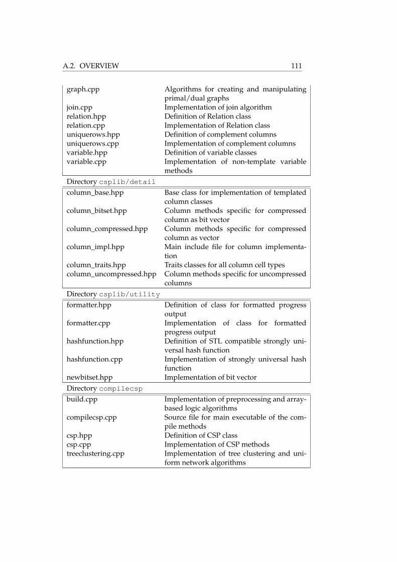
A.2. OVERVIEW 111
graph.cpp Algorithms for creating and manipulatingprimal/dual graphs
join.cpp Implementation of join algorithmrelation.hpp Definition of Relation classrelation.cpp Implementation of Relation classuniquerows.hpp Definition of complement columnsuniquerows.cpp Implementation of complement columnsvariable.hpp Definition of variable classesvariable.cpp Implementation of non-template variable
methodsDirectory csplib/detail
column_base.hpp Base class for implementation of templatedcolumn classes
column_bitset.hpp Column methods specific for compressedcolumn as bit vector
column_compressed.hpp Column methods specific for compressedcolumn as vector
column_impl.hpp Main include file for column implementa-tion
column_traits.hpp Traits classes for all column cell typescolumn_uncompressed.hpp Column methods specific for uncompressed
columnsDirectory csplib/utility
formatter.hpp Definition of class for formatted progressoutput
formatter.cpp Implementation of class for formattedprogress output
hashfunction.hpp Definition of STL compatible strongly uni-versal hash function
hashfunction.cpp Implementation of strongly universal hashfunction
newbitset.hpp Implementation of bit vectorDirectory compilecsp
build.cpp Implementation of preprocessing and array-based logic algorithms
compilecsp.cpp Source file for main executable of the com-pile methods
csp.hpp Definition of CSP classcsp.cpp Implementation of CSP methodstreeclustering.cpp Implementation of tree clustering and uni-
form network algorithms

APPENDIX A. SOURCE CODE 112
Directory cspruntime
cspruntime.cpp Source for main executable of the runtimemethods
runtime_network.hpp Definition of class RuntimeNetworkruntime_network.cpp Implementation of fundamental operationssimulatorui.hpp Definition of simple console based interac-
tive constraint solversimulatorui.cpp Implementation of simple console based in-
teractive constraint solver
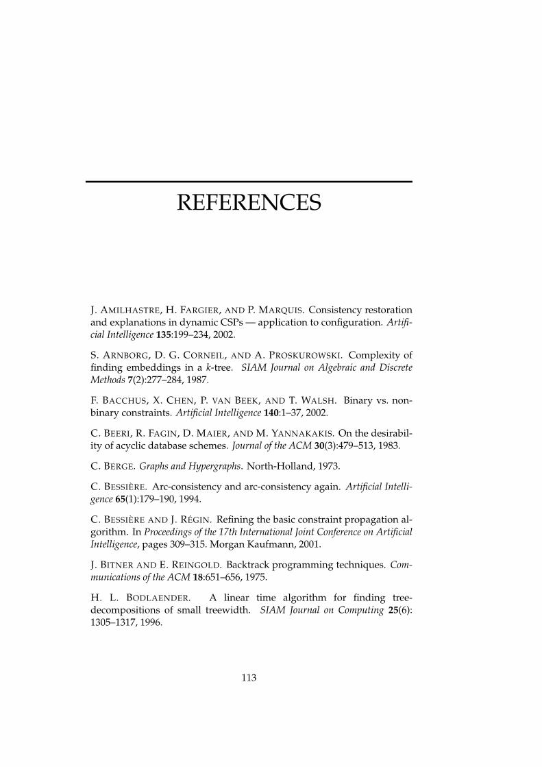
REFERENCES
J. AMILHASTRE, H. FARGIER, AND P. MARQUIS. Consistency restorationand explanations in dynamic CSPs — application to configuration. Artifi-cial Intelligence 135:199–234, 2002.
S. ARNBORG, D. G. CORNEIL, AND A. PROSKUROWSKI. Complexity offinding embeddings in a k-tree. SIAM Journal on Algebraic and DiscreteMethods 7(2):277–284, 1987.
F. BACCHUS, X. CHEN, P. VAN BEEK, AND T. WALSH. Binary vs. non-binary constraints. Artificial Intelligence 140:1–37, 2002.
C. BEERI, R. FAGIN, D. MAIER, AND M. YANNAKAKIS. On the desirabil-ity of acyclic database schemes. Journal of the ACM 30(3):479–513, 1983.
C. BERGE. Graphs and Hypergraphs. North-Holland, 1973.
C. BESSIÈRE. Arc-consistency and arc-consistency again. Artificial Intelli-gence 65(1):179–190, 1994.
C. BESSIÈRE AND J. RÉGIN. Refining the basic constraint propagation al-gorithm. In Proceedings of the 17th International Joint Conference on ArtificialIntelligence, pages 309–315. Morgan Kaufmann, 2001.
J. BITNER AND E. REINGOLD. Backtrack programming techniques. Com-munications of the ACM 18:651–656, 1975.
H. L. BODLAENDER. A linear time algorithm for finding tree-decompositions of small treewidth. SIAM Journal on Computing 25(6):1305–1317, 1996.
113

REFERENCES 114
H. L. BODLAENDER, A. M. C. A. KOSTER, AND F. VAN DEN EIJKHOF. Pre-processing rules for triangulation of probabilistic networks. Technical Re-port UU-CS-2003-001, Institute for Information and Computing Sciences,Utrecht University, 2003.
P. A. BONCZ, S. MANEGOLD, AND M. L. KERSTEN. Database architectureoptimized for the new bottleneck: Memory access. The VLDB Journal 9:231–246, 2000.
F. BOUQUET AND P. JÉGOU. Using OBDDs to handle dynamic constraints.Information Processing Letters 67(1):111–120, 1997.
F. BRGLEZ AND H. FUJIWARA. A neutral netlist of 10 combinationalbenchmark circuits and a target translator in fortran. In Proceedings of In-ternational Symposium on Circuits and Systems, pages 663–698, 1985.
R. E. BRYANT. Graph-based algorithms for Boolean function manipula-tion. IEEE Transactions on Computers C-35(8):677–691, 1986.
E. F. CODD. A relational model of data for large shared data banks. Com-munications of the ACM 13(6):377–387, 1970.
M. C. COOPER. An optimal k-consistency algorithm. Artificial Intelligence41(1):89–95, 1989.
T. H. CORMEN, C. E. LEISERSON, R. L. RIVEST, AND C. STEIN. Introduc-tion to Algorithms. MIT Press, 2nd edition, 2001.
G. B. DANTZIG. Linear Programming and Extensions. Princeton UniversityPress, 1963.
J. DE KLEER AND G. J. SUSSMAN. Propagation of constraints applied tocircuit synthesis. Circuit Theory and Applications 8:127–144, 1980.
R. DECHTER. Bucket elimination: a unifying framework for processinghard and soft constraints. ACM Computing Surveys 28A(4), 1996.
R. DECHTER AND A. DECHTER. Belief maintenance in dynamic constraintnetworks. In Proceedings of the 7th Annual Conference of the American Asso-ciation of Artificial Intelligence, pages 37–42. AAAI Press/MIT Press, 1988.
R. DECHTER AND J. PEARL. Tree clustering for constraint networks. Arti-ficial Intelligence 38(3):353–366, 1989.
Y. EL FATTAH AND R. DECHTER. An evaluation of structural parametersfor probabilistic reasoning: Results on benchmark circuits. In Proceedingsof the 12th Annual Conference on Uncertainty in Artificial Intelligence, pages244–251. Morgan Kaufmann, 1996.

REFERENCES 115
C. ERBAS, S. SARKESHIK, AND M. M. TANIK. Different perspectives ofthe n-queens problem. In Proceedings of the 1992 ACM Annual Conferenceon Communications, pages 99–108. ACM Press, 1992.
F. FRAYMAN. User-interaction requirements and its implications for ef-ficient implementations of interactive constraint satisfaction systems. InWorking Notes of the 1st International Workshop on User-Interaction in Con-straint Satisfaction, pages 31–41, 2001.
E. C. FREUDER. Synthesizing constraint expressions. Communications ofthe ACM 21(11):958–966, 1978.
E. C. FREUDER. A sufficient condition for backtrack-free search. Journal ofthe ACM 29(1):24–32, 1982.
E. C. FREUDER. Eliminating interchangeable values in constraint satis-faction problems. In Proceedings of the 9th National Conference on ArtificialIntelligence, pages 227–233. AAAI Press/MIT Press, 1991.
M. R. GAREY AND D. S. JOHNSON. Computers and Intractability – A Guideto the Theory of NP-Completeness. W. H. Freeman, 1979.
J. GASCHNIG. Performance measurement and analysis of search algo-rithms. Technical Report CMU-CS-79124, Carnegie Mellon University,1979.
I. GENT, E. MACINTYRE, P. PROSSER, P. SHAW, AND T. WALSH. Theconstrainedness of arc consistency. In Proceedings of the 3rd InternationalConference on Principles and Practice of Constraint Programming, pages 327–340. Springer-Verlag, 1997.
A. GEORGE AND J. LIU. The evolution of the minimum degree orderingalgorithm. SIAM Review 31(1):1–19, 1989.
G. GOTTLOB, N. LEONE, AND F. SCARCELLO. Hypertree decompositionsand tractable queries. In Proceedings of the 18th ACM Symposium on Princi-ples of Database Systems, pages 21–32. ACM Press, 1999a.
G. GOTTLOB, N. LEONE, AND F. SCARCELLO. On tractable queries andconstraints. In Database and Expert Systems Applications, 10th InternationalConference, volume 1677 of Lecture Notes in Computer Science, pages 1–15.Springer Verlag, 1999b.
G. GOTTLOB, N. LEONE, AND F. SCARCELLO. A comparison of structuralCSP decomposition methods. Artificial Intelligence 124(2):243–282, 2000.
M. GYSSENS, P. JEAVONS, AND D. COHEN. Decomposing constraint sat-isfaction problems using database techniques. Artificial Intelligence 66(1):57–89, 1994.

REFERENCES 116
T. HAGERUP. Sorting and searching on the word RAM. In Proceedings ofthe 15th Annual Symposium on Theoretical Aspects of Computer Science, vol-ume 1373 of Lecture Notes in Computer Science, pages 366–398. Springer-Verlag, 1998.
T. HAGERUP, P. B. MILTERSEN, AND R. PAGH. Deterministic dictionaries.Jorunal of Algorithms 41(1):69–85, 2001.
C. HAN AND C. LEE. Comments on Mohr and Henderson’s path consis-tency algorithm. Artificial Intelligence 36(1):125–130, 1988.
C. A. R. HOARE. Essays in Computing Science. Prentice-Hall, 1989.
P. D. HUBBE AND E. C. FREUDER. An efficient cross product representa-tion of the constraint satisfaction problem search space. In Proceedings ofthe 10th National Conference on Artificial Intelligence, pages 421–427. AAAIPress/MIT Press, 1992.
J. KATAJAINEN AND J. N. MADSEN. Performance tuning an algorithmfor compressing relational tables. In Proceedings of the 8th ScandinavianWorkshop on Algorithm Theory, volume 2368 of Lecture Notes in ComputerScience, pages 398–407. Springer-Verlag, 2002.
V. KLEE AND G. J. MINTY. How good is the simplex algorithm? InInequalities III. Proceedings of the 3rd Symposium on Inequalities, pages 159–175. Academic Press, 1972.
G. KONDRAK AND P. VAN BEEK. A theoretical evaluation of selected back-tracking algorithms. Artificial Intelligence 89:365–387, 1997.
V. KUMAR. Algorithms for constraints satisfaction problems: A survey.AI Magazine 13(1):32–44, 1992.
A. K. MACKWORTH. On reading sketch maps. In Proceedings of the 5th In-ternational Joint Conference on Artificial Intelligence, pages 598–606. WilliamKaufmann, 1977a.
A. K. MACKWORTH. Consistency in networks of relations. Artificial Intel-ligence 8(1):99–118, 1977b.
J. N. MADSEN. Algorithms for compressing and joining relations. CPHSTL Report 2002-1, Department of Computing, University of Copen-hagen, 2002. Available at http://www.cphstl.dk .
D. MAIER. The Theory of Relational Databases. Computer Science Press,1983.
J. MCHUGH. Holy cow, no one’s done this! Forbes 57(11):122–128, 1996.

REFERENCES 117
W. MENZEL. Constraint satisfaction for robust parsing of spoken lan-guage. Journal of Experimental and Theoretical Artificial Intelligence 10(1):77–89, 1998.
N. C. MEYERS. Traits: A new and useful template technique. C++ Report7, 1995. Available at http://www.cantrip.org/traits.html .
I. MIGUEL AND Q. SHEN. Hard, flexible and dynamic constraint satisfac-tion. Knowledge Engineering Review 14(3):199–220, 1999.
I. MIGUEL AND Q. SHEN. Solution techniques for constraint satisfactionproblems: foundations. Artificial Intelligence Review 15(4):243–267, 2001a.
I. MIGUEL AND Q. SHEN. Solution techniques for constraint satisfactionproblems: advanced approaches. Artificial Intelligence Review 15(4):269–293, 2001b.
S. MITTAL AND B. FALKENHAINER. Dynamic constraint satisfaction prob-lems. In Proceedings of the 8th National Conference on Artificial Intelligence,pages 25–32. AAAI Press/The MIT Press, 1990.
R. MOHR AND T. C. HENDERSON. Arc and path consistency revisited.Artificial Intelligence 28(2):225–233, 1986.
G. L. MØLLER. On the Technology of Array-Based Logic. Ph. D. the-sis, Technical University of Denmark, 1995. Available at http://www.arraytechnology.com/documents/lic.pdf .
U. MONTANARI. Network of constraints: Fundamental properties andapplications to picture processing. Information Sciences 7:95–132, 1974.
T. MORE, JR. Axioms and theorems for a theory of arrays. IBM Journal ofResearch and Development 17(2):135–175, 1973.
J. NIELSEN. Usability Engineering. Morgan Kaufmann, 1994.
J. PEARSON AND P. JEAVONS. A survey of tractable constraint satisfactionproblems. Technical Report CSD-TR-97-15, Royal Holloway University ofLondon, 1997.
N. ROBERTSON AND P. D. SEYMOUR. Graph minors. II. Algorithmic as-pects of tree-width. Journal of Algorithms 7(3):309–322, 1986.
D. SABIN AND E. C. FREUDER. Contradicting Conventional Wisdom inConstraint Satisfaction. In Proceedings of the 2nd International Workshopon Principles and Practice of Constraint Programming, volume 874 of LectureNotes in Computer Science, pages 10–20. Springer-Verlag, 1994.
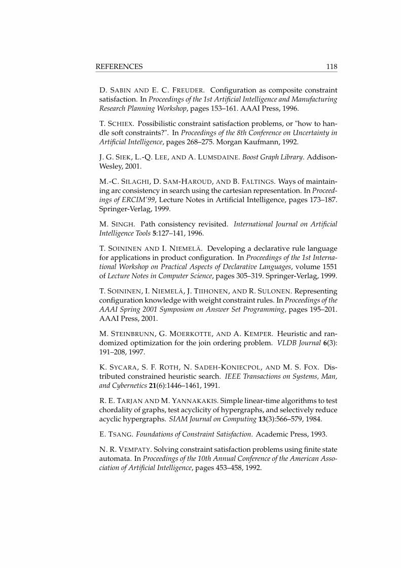
REFERENCES 118
D. SABIN AND E. C. FREUDER. Configuration as composite constraintsatisfaction. In Proceedings of the 1st Artificial Intelligence and ManufacturingResearch Planning Workshop, pages 153–161. AAAI Press, 1996.
T. SCHIEX. Possibilistic constraint satisfaction problems, or "how to han-dle soft constraints?". In Proceedings of the 8th Conference on Uncertainty inArtificial Intelligence, pages 268–275. Morgan Kaufmann, 1992.
J. G. SIEK, L.-Q. LEE, AND A. LUMSDAINE. Boost Graph Library. Addison-Wesley, 2001.
M.-C. SILAGHI, D. SAM-HAROUD, AND B. FALTINGS. Ways of maintain-ing arc consistency in search using the cartesian representation. In Proceed-ings of ERCIM’99, Lecture Notes in Artificial Intelligence, pages 173–187.Springer-Verlag, 1999.
M. SINGH. Path consistency revisited. International Journal on ArtificialIntelligence Tools 5:127–141, 1996.
T. SOININEN AND I. NIEMELÄ. Developing a declarative rule languagefor applications in product configuration. In Proceedings of the 1st Interna-tional Workshop on Practical Aspects of Declarative Languages, volume 1551of Lecture Notes in Computer Science, pages 305–319. Springer-Verlag, 1999.
T. SOININEN, I. NIEMELÄ, J. TIIHONEN, AND R. SULONEN. Representingconfiguration knowledge with weight constraint rules. In Proceedings of theAAAI Spring 2001 Symposiom on Answer Set Programming, pages 195–201.AAAI Press, 2001.
M. STEINBRUNN, G. MOERKOTTE, AND A. KEMPER. Heuristic and ran-domized optimization for the join ordering problem. VLDB Journal 6(3):191–208, 1997.
K. SYCARA, S. F. ROTH, N. SADEH-KONIECPOL, AND M. S. FOX. Dis-tributed constrained heuristic search. IEEE Transactions on Systems, Man,and Cybernetics 21(6):1446–1461, 1991.
R. E. TARJAN AND M. YANNAKAKIS. Simple linear-time algorithms to testchordality of graphs, test acyclicity of hypergraphs, and selectively reduceacyclic hypergraphs. SIAM Journal on Computing 13(3):566–579, 1984.
E. TSANG. Foundations of Constraint Satisfaction. Academic Press, 1993.
N. R. VEMPATY. Solving constraint satisfaction problems using finite stateautomata. In Proceedings of the 10th Annual Conference of the American Asso-ciation of Artificial Intelligence, pages 453–458, 1992.

REFERENCES 119
R. J. WALLACE. Why AC-3 is almost always better than AC-4 for es-tablishing arc consistency in CSPs. In Proceedings of the 13th InternationalJoint Conference on Artificial Intelligence, pages 239–245. Morgan Kaufmann,1993.
R. WEIGEL AND B. FALTINGS. Compiling constraint satisfaction prob-lems. Artificial Intelligence 115(2):257–287, 1999.
K. WEIHE. Covering trains by stations or the power of data reduc-tion. In Online Proceedings of the 1st Workshop on Algorithms and Experi-ments, 1998. Available at http://rtm.science.unitn.it/alex98/proceedings.html .
M. YANNAKAKIS. Computing the minimum fill-in is NP-complete. SIAMJournal of Algebraic and Discrete Methods 2:77–79, 1981.
B. YU AND H. J. SKOVGAARD. A configuration tool to increase productcompetitiveness. IEEE Intelligent Systems 13(4):34–41, 1998.

REFERENCES 120

LIST OF FIGURES
1.1 Graph 3-colorability examples. . . . . . . . . . . . . . . . . . 31.2 A solution to the 8-queen problem. . . . . . . . . . . . . . . . 41.3 An example of an online store. . . . . . . . . . . . . . . . . . 71.4 A high level view of a configuration system. . . . . . . . . . 8
2.1 Applying projection and join operations. . . . . . . . . . . . 16
3.1 Some consistent instantiations of the 4-queen problem. . . . 213.2 Different graph representations of a constraint network. . . . 253.3 Search tree example for an unsatisfiable network. . . . . . . 283.4 A graph ordering example. . . . . . . . . . . . . . . . . . . . 34
5.1 Intermediate results when joining relations. . . . . . . . . . . 635.2 A relation stored using the normal and the Cartesian product
representation. . . . . . . . . . . . . . . . . . . . . . . . . . . . 645.3 Joining relations stored using the Cartesian product repre-
sentation. . . . . . . . . . . . . . . . . . . . . . . . . . . . . . . 665.4 Example of the tree clustering method. . . . . . . . . . . . . . 695.5 Fundamental operations in a CPR network with a single con-
straint. . . . . . . . . . . . . . . . . . . . . . . . . . . . . . . . 745.6 CPR network with a two constraints. . . . . . . . . . . . . . . 74
6.1 Constraint graphs for instance ns11. . . . . . . . . . . . . . . 826.2 Constraint graphs for circuit c432. . . . . . . . . . . . . . . . 846.3 Constraint graphs for the pigeon hole problem for h = 6. . . 866.4 Constraint graphs for the 8-queen problem. . . . . . . . . . . 87
7.1 Splitting the relation in Figure 7.1(a). . . . . . . . . . . . . . . 987.2 Splitting a relation stored in the CPR. . . . . . . . . . . . . . . 99
121

LIST OF FIGURES 122
7.3 Constructing a uniform acyclic network. . . . . . . . . . . . . 101

LIST OF TABLES
3.1 Constraint and database terminology. . . . . . . . . . . . . . 21
4.1 Complexity results for the fundamental operations. . . . . . 59
6.1 Characteristics of configuration problem instances. . . . . . . 836.2 ISCAS ’85 benchmark circuits. . . . . . . . . . . . . . . . . . . 836.3 Characteristics of circuit verification problem instances. . . . 856.4 Characteristics of satisfiability problem instances. . . . . . . 856.5 Characteristics of puzzle problem instances. . . . . . . . . . . 866.6 Compilation results using array-based logic. . . . . . . . . . 896.7 Compilation results using the tree clustering method. . . . . 906.8 Results of running simulations of ADD-CONSTRAINT. . . . . 90
7.1 Complexity results for the fundamental operations in a uni-form acyclic network. . . . . . . . . . . . . . . . . . . . . . . . 97
7.2 Compilation results for creating a uniform acyclic network. . 1037.3 Results of running simulations of ADD-CONSTRAINT on the
uniform acyclic network. . . . . . . . . . . . . . . . . . . . . . 103
A.1 Packages required for compilation. . . . . . . . . . . . . . . . 110
123

LIST OF TABLES 124
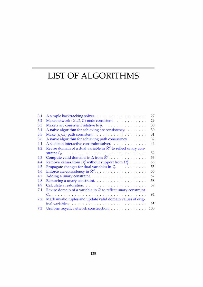
LIST OF ALGORITHMS
3.1 A simple backtracking solver. . . . . . . . . . . . . . . . . . . 273.2 Make network (X, D, C) node consistent. . . . . . . . . . . . 293.3 Make x arc consistent relative to y. . . . . . . . . . . . . . . . 303.4 A naive algorithm for achieving arc consistency. . . . . . . . 303.5 Make (i, j, k) path consistent. . . . . . . . . . . . . . . . . . . . 313.6 A naive algorithm for achieving path consistency. . . . . . . 324.1 A skeleton interactive constraint solver. . . . . . . . . . . . . 444.2 Revise domain of a dual variable in Rd to reflect unary con-
straint Cx. . . . . . . . . . . . . . . . . . . . . . . . . . . . . . 524.3 Compute valid domains in ∆ from Rd. . . . . . . . . . . . . . 534.4 Remove values from Dd
S without support from DdT. . . . . . . 55
4.5 Propagate changes for dual variables in Q. . . . . . . . . . . 554.6 Enforce arc-consistency in Rd. . . . . . . . . . . . . . . . . . . 554.7 Adding a unary constraint. . . . . . . . . . . . . . . . . . . . 574.8 Removing a unary constraint. . . . . . . . . . . . . . . . . . . 584.9 Calculate a restoration. . . . . . . . . . . . . . . . . . . . . . . 597.1 Revise domain of a variable in R to reflect unary constraint
Cx. . . . . . . . . . . . . . . . . . . . . . . . . . . . . . . . . . . 947.2 Mark invalid tuples and update valid domain values of orig-
inal variables. . . . . . . . . . . . . . . . . . . . . . . . . . . . 957.3 Uniform acyclic network construction. . . . . . . . . . . . . . 100
125


