Methods for Predicting Dispersion Coefficients in Nat ural Streams, with Applications to Lower Reaches of the Green and Duwamish Rivers Washington GEOLOGICAL SURVEY PROFESSIONAL PAPER 582-A Prepared in cooperation with the Municipality of Metropolitan Seattle
Transcript
Methods for Predicting Dispersion Coefficients in Nat ural Streams, with Applications to Lower Reaches of the Green and Duwamish Rivers Washington
GEOLOGICAL SURVEY PROFESSIONAL PAPER 582-A
Prepared in cooperation with the
Municipality of Metropolitan Seattle
Methods for Predicting Dispersion Coefficients in Natural Streams, with Applications to Lower Reaches of the Green and Duwamish Rivers Washington By HUGO B. FISCHER
DISPERSION IN SURFACE WATER
GEOLOGICAL SURVEY PROFESSIONAL PAPER 582-A
Prepared in cooperation with the
Municipality of Metropolitan Seattle
UNITED STATES GOVERNMENT PRINTING OFFICE, WASHINGTON : 1968
UNITED STATES DEPARTMENT OF THE INTERIOR
STEWART L. UDALL, Secretary
GEOLOGICAL SURVEY
William T. Pecora, Director
For sale by the Superintendent of Documents, U.S: Government Printing Office Washington, D.C. 20402 - Price 30 cents (paper cover)
Longitudinal dispersion studies in the Green and Duwamish Rivers-Continued
Purpose and procedure _________________________ _ Acknowledgments ______________________________ _
Visual and photographic observations ____________ _
Diffusion versus dispersion __________________________ _ Analytical prediction of the dispersion coefficient ______ _
Longitudinal dispersion studies in the Green and Du-Theoretical analysis ____________________________ _ Application to the Green and Duwamish Rivers ___ _
Results _________________________ . ______________ _ Description of the study reach ___________________ _ Measurement techniques ________________________ _
Numerical prediction of the dispersion coefficient ______ _ Conclusions _______________________________________ _
Experiments of August 3-4 and September 9 ______ _ References ________________________________________ _
ILLUSTRATIONS
FIGURE 1. Index map of the Orillia Bridge-Boeing Bridge study reach, Green and Duwamish Rivers, showing dye injection point, river sections, and area covered by aerial photographs ______________________________________________________________ _
2. Photographs of Green and Duwamish River channel at river sections _____ ----------3. River-channel sections at sampling stations ___________________ -_----------------4. Graphs showing forecast tides at Seattle, August 3-4 and September 9, and times of
5-6. Graphs showing changes in dye concentration, velocity, and river stage at sampling stations-
5. August 3-4----------------------------------------------------------6. September 9---------------------------------------------------------
7. Graph showing observed longitudinal distribution of dye at selected times, August 3 __ -8. Graph showing changes in the variance of dye distribution, August 3-4 and September 9_
9-10. Graphs comparing observed and predicted longitudinal distribution of dye-9. August 3, 1500 hours _______________________________ ------------------
10. September 9, 1100 hours _________________________________ -------------11. Aerial photographs of dye dispersion, August 17 ________________________________ _ 12. Map showing area covered by photographs in figure 11---------------------------13. Schematic aerial view of dye cloud at Cherry Street, 1550 hours, August 3 ___ -------
14-15. River-channel sections showing lines of equal velocity, August 31-14. At Renton Junction, 1230 hours _______________________________________ _ 15. At Foster Golf Course, 1530 hours _____________________________________ _
16-17. Graphs showing changes in dye concentrations at several lateral stations, August 31-16. At Renton Junction _________________________________________________ _ 17. At Foster Golf Course _____________________________ -------------------
18-19. Graphs showing changes in mean dye-concentration gradient, mass transport, and dispersion coefficient, August 31-
18. At Renton Junction _________________________________________________ _ 19. At Foster Golf Course ______________________________ ------------------
20. Graph comparing observed and predicted lateral distributions of dye at Renton Junc-tion at selected times, August 3L ___________________________________________ _
21. Schematic section showing division of flow into stream tubes ____________ ----------22. Graph showing computer-predicted variance of mean concentration distribution as a
function of time ______________________________________________ -------------
Page
A3 5 6
7
8 9
10 11
11 13 14 15 16
19 19
20 20
21 21
22 23
24
III
Page
A13 17 17 18 18 22 25 27
IV
FIGURE
CONTENTS
Page
23. Graph comparing computer-predicted surface, bottom, and average longitudinal dis-tributions of concentration__________________________________________________ A24
24. Graph comparing observed and computer-predicted variances of mean dye-concen-tration distribution_________________________________________________________ 25
25. Graph comparing observed and computer-predicted longitudinal distributions of mean dye concentration 155 minutes after injection, August 3L_______________________ 25
26-27. Graphs comparing observed and computer-predicted lateral distributions of dye at Renton Junction, August 31-
TABLE 1. Observation sections used during the four experiments and type of information ob-tained____________________________________________________________________ A4
DISPERSION IN SURFACE WATER
METHODS FOR PREDICTING DISPERSION COEFFICIENTS IN NATURAL STREAMS, WITH APPLICATIONS TO LOWER REACHES OF THE GREEN AND
DUWAMISH RIVERS, WASHINGTON
By HuGo B. FISCHER
ABSTRACT
Four dye dispersion experiments were conducted in the Green and Duwamish Rivers, Wash. Longitud.iual dispersion coefficients were obtained in two experiments, lateral concentration variations in the third, and aerial photographs in the fourth. The study reach was a section of meandering river, most of which is affected by tides during a part of the tidal cycle. Dispersion was observed during normal riverflow and tidal reversals. In normal :flow of about 300 cfs the observed dispersion coefficient was 70-90 fe per sec.
In natural riverflow, lateral variation in velocity is hypothesized to be the dominant mechanism for dispersion. With this hypothesis, G. I. Taylor's theory for turbulent dispersion in pipes may be applied to natural streamflow. The resulting analySis predicts a dispersion coefficient of 88 ft2 per sec for a :flow of 300 cfs in the Green and Duwamish Rivers.
A numerical ·SOlution to ·the convective diffusion equation is obtained, utilizing a high-speed electronic computer. Analysis of a two-dimensional flow with logarithmic velocity pro:file, for which a theoretical result is a vaila'b1e, shows that the program produces accurate results. Analysis of the flow in the Green and Duwamish Rivers predicts a dispersion coefficient of 91 fe per 'Sec.
The analyses herein presented, both analytical and numerical, provide two ways of predicting a dispersion coefficient for a natural stream. The prediction requires :field measurement of channel geometry, shear stress, and cross-sectional distribution of velocity only. Hopefully, future field experiments will further confirm the two prediction methods.
INTRODUCTION
PURPOSE AND PROCEDURE
In a fundamental pap~r, Taylor (1954) established that longitudinal dispersion in a long, straight pipe may be characterized by a one-dimensional classical <liffusion equation, in which the diffusive and convective processes occurring throughout the cross section interact to produce a longitudinal dispersion coefficient. Although Taylor specifically stated that his analysis applied only to flow in a long, straight pipe, many investigators have subsequently attempted to apply the same concept to flows in open channels, in both labora-
I tory flumes and natural streams. Thomas (1958) succeeded in applying Taylor's concept to flow in an infinitely wide two-dimensional open channel in which the flow is described by a power-law velocity distribution. He obtained a complicated funotional relationship, whose behavior is not obvious without detailed reading of his unpublished thesis. A plot of his resulting dispersion coefficient as a function of Reynolds number has been given by Fischer (1965). Elder (1959) duplicated Thomas' effort, for assuming a logarithmic velocity profile, and obtained a remarkably simple result :
D=5.93 dU*, (1)
in which D is the longitudinal one-dimensional dispersion coefficient, d is the depth of flow, U* is the shear velocity, and the von Karman constant has been assumed equal to 0.41. Elder succeeded in verifying his formula in a very small flume. However, more recent investigators, in both laboratories and natural streams, have obtained very much greater values of D. Laboratory investigations by Glover (1964) have yielded values of Don the order of 20 dU*. Values obtained in natural streams have ranged from 40 to 800 dU*, the average being around 200 d U*. The large variation in results has cast doubt on the applicability of Taylor's analysis to open channel flows, at the same time spawning considerable interest in what factors actually do produce dispersion.
Recently, Fischer (1966a) has suggested that Taylor's analysis does not correctly describe the entire dispersion process in natural streams. Two periods are identified : an initial period following insertion of a pollutant, limited not only to the period of cross-sectional mixing but involving possibly several miles of streamflow as 'veil, in which a longitudinally skewed cloud is formed; and a later period, during which Taylor's analysis applies and the initial distribution
Al
A2 DISPERSION IN SURFACE WATER
dooays according to the diffusion equation. Only in the later "Taylor" period is it permissible to speak of a dispersion coefficient which correctly describes the process. The approximations involved in Taylor's analysis and the duration of the initial convective period have been discussed in more detail by Fischer (1966b).
A major purpose of this report is to show that in spite of the initial non-Taylor period and in spite of the variety of field results already mentioned, Taylor's basic reasoning is sufficiently valid to provide a method whereby dispersion coefficients in natural streams may be predicted. Such a method is described and used to make a reasonably accurate prediction for the river under study.
The study herein described was conducted as part of a cooperative project with the Municipality of Metropolitan Seattle, whose Renton Sewage Treatment Plant discharges treated se,vage into the Duwamish River near the upstream end of the study reach. The investigation had a twofold purpose : first, to provide an exact description of the movement and dispersion of the sewage effluent in the study reach; and second, to make a detailed investigation of the basic mechanics of dispersion in a natural environment. The study consisted of four experiments; the experiments of August 3-4 and September 9, 1965, are described as longitudinal dispersion experiments, during which dye was injected upstream from the study reach, and a series of observation stations were established at river sections throughout the reach. The experiment of August 17 was similar to that of August 3-4, 1965, except that observations were limited to a few stations, and the dye cloud was photographed from the air at intervals throughout the day. The experiment of August 21 was designed to investigate the role of lateral concentration gradients and to show their importance in the dispersion process.
ACKNOWLEDGMENTS
The theory underlying this study was derived by the author while a graduate student at the California Institute of Technology, Pasadena, Calif. The stimulation and helpful suggestions of Dr. Norman H. Brooks and the financial suppqrt of fellowships under the National Defense Education Act and from the Fannie and John Hertz Foundation are gratefully acknowledged.
The investigation was conducted by the Washington District of the U.S. Geological Survey's Water Resources Division under L. B. Laird, District Chief, and J. F. Santos, Project Chief. The author expresses his appreciation to the many members of the district staff who participated with him in data collection and analySIS.
DIFFUSION VERSUS DISPERSION
A question frequently asked is, "What is the difference between diffusion and dispersion~" More than semantics is involved; both processes concern the spreading out of particles that are initiaUy at the same point, but a significant difference exists in the degree of randomness of the motion.
The ~rm "diffusion" is generally applied to processes in' which the motion of the particles is entirely random, with or without some autocorrelation. The spreading out is accomplished by the .different pat~s randomly selected by the different particles. In one dimension, the classical problem is generally referred to as the "Drunkard's walk" problem. An infinite population of particles originate a one-dimensional motion from a single point at the same time. After each interval of time, t::..t, ea,ch particle moves one step length t::..l, but whether the step be forward or backwa.rd is entirely random. If a limit is taken where both the time interval and step length shrink to zero, but the ratio ( t::..l) 2 I t::..t remains finite, it may be shown mathematically that the distribution of particles is described by the FokkerPlank equation, or diffusion equation,
oc o2c at =D aw2'
in which tis time, w is the longitudinal coordinate, D is a coefficient depending on the ratio of ( t::..l) 2 to t::..t, and o is the concentration of particles per unit length.
Dispersion also involves a process of spreading out, but with the help of some mechanism other than random motion. For instance, suppose that the randomly walking "drunks" of the previous exa.mple are getting on and off of busses in a random way, but that the busses operate on a fixed schedule. The motion is still random, but the final distribution of "drunks" depends strongly on the bus schedule. Very likely, it does not obey the diffusion equation.
Dispersion in a river is very similar to the "d~unk on a bus" problem. An element of randomness exists; namely, the cross-sectional turbulent diffusion (turbulence generally being thought of as a completely random motion, and diffusion therefore being the proper term). The bus schedule is analogous to the ~ariati?n of longitudinal velocities within the cross sectiOn. Dispersion is caused primarily by "~ussing" of t?~ particles, that is, convection at the different velocities of different stream lines. The primary effect of the turbulence is to cause the particles to "change busses."
Strictly speaking, as Batchelor ( ~964 ). has p~inted out the motion of each water particle In a uniform str~am is a stationary random function. H~wever, ~n the stream the primary mechanism for spreading out Is the
METHODS FOR PREDICTING DISPERSION COEFFICIENTS-GREEN AND DUW AMISH RIVERS, WASH. A3
time-steady cross-sectional variation of velocity (the different busses) . In contrast, in turbulent (or eddy) diffusion, the only mechanism is random temporal velocity variations (random. steps forward or backward) . As discussed below, the spatial velocity variations in a stream are far more effective at spreading out than are the temporal variations. Since both the mechanisms and results are so different, the terms "dispersion," for spreading out due to spatial velocity differences, and "diffusion," for spreading by random temporal fluctuations, should not be interchanged.
LONGITUDINAL DISPERSION STUDIES IN THE GREEN AND DUWAMISH RIVERS
DESCRIPTION OF THE STUDY REACH
The Green River rises in the Cascade Mountains just north of Mount Rainier. It flows through the foothill area and emerges onto an alluvial valley at Auburn, Wash. From Auburn until its discharge into Elliott Bay at Seattle, it meanders through the flat alluvial valley. The downstream end, below the confluence of the Black River and comprising mostly the estuary, is known as the Duwamish River. The Black River, once a major tributary, since 1917 has had hardly any flow; this channel realinement and the geology of the area have been described by Mullineaux (1961).
The reach of interest (fig. 1) includes the lowest 13 miles of the Green-Duwamish system, commencing at the Renton Junction Bridge and continuing to Elliott Bay. The tidal range at Elliott Bay averages about 10 feet, although a maximum of 16 feet has been recorded. In its lowest 6 miles, the estuary has been dredged to a depth of 20 feet, varies in width from 400 to 1,000 feet, and may be characterized as a one-dimensional estuary. The upper 7-mile reach, which is the range of primary interest for this study, may be characterized as a meandering, tidally influenced river. At low flows, about 300 cfs (cubic feet per second) or less, the stage at the uppermost section shows tidal influence for tides of 8 feet or more at Seattle. Reverse flow occurs at higher tides. Thus, during most high tides the entire study reach is tidally affected. In contrast, much of the reach flows as a normal river at low tide.
Flow in the Green River at Auburn (U.S. Geol. Survey gaging station 12-1130), 16.6 miles above Orillia Bridge, varies from about 12,000 cfs at flood stage, often recorded during winter floods, to low flows on the order of 200-300 cfs. The river is regulated upstream from Auburn by Howard A. Hanson Dam, operated by the U.S. Army Corps of Engineers to maintain a low-flow discharge of at least 80 cfs. From Auburn to the mouth the river is leveed to a height of 20 feet. Most of th~
122° 17'30" 122°15'
0 lfz 2 MILES
FIGURE 1.-Index map of the Orillia Bridge-Boeing Bridge study reach, Green and Duwamish Rivers, showing dye injection point, river sections, and area covered by aerial photographs (fig. 12).
sediment transport and channel degradation takes place during the winter floods, when the river often flows nearly bank full. The present study was conducted during particularly low flows because of the primary interest in pollution. At low stage, the river is confined to a bottom having banks of mud, sand, or in places riprap; the upper banks are covered with grass and blackberry vines. The river contains debris of all sorts, including snags, logs, and car bodies, much of which projects above the surface at low stage and adds to the channel roughness.
The slope of the river between Renton Junction and 42d Street, computed for low tide on August 3, was 0.000224. A mean hydraulic radius for this reach is estimated at 3.6 feet, yielding a shear velocity of 0.161
A4 DISPERSION IN SURFACE WATER
fps (foot per second) , a Darcy-W eisbach friction factor of 0.26, and a Manning n of 0.058. The Manning n value agrees well with a table by Rouse ( 1950).
Table 1 gives all sampling and measuring locations used in the study and the types of information collected at each section. The river sections, in feet upstream from
the mouth of the estuary, were established by measuring on the U.S. Geological Survey map titled "Seattle and Vicinity," at a scale of 1:62,500. Figure 2 shows general views of the river sections. Stream depths at several
I of the cross sections, which are shown in figure 3, were observed on August 3.
TABLE !.-Observation sections used during the four experiments and type of information obtained (Abbreviations: Auto., automatic stage recorder; Sta., station, with lateral distance in feet, from arbitrary point; WWG, wire-weight gage]
Distance August3-4 August 17 August 31 September9
River cross sections upstream
from mouth of Dye Velocity Stage Dye Dye Dye Velocity Stage estuary (feet)
145 __ }wwa Boeing Bridge ________ 34, 320 Sta. 170 _____ Sta. 170_ Hand -------- ------------ -------- --------
line.
MEASUREMENT TECHNIQUES
The tracer used was Rhodamine B, a commercial dye whose properties have been summarized by Buchanan ( 1964). For this study, the primary properties of int~,rest are that: (1) the dye is miscible in water up to concentrations of 2 percent by weight; ( 2) it would not decay appreciably during the duration of the test; and (3) it is capable of being adsorbed onto river sediments, although in unknown quantities. In this study the dye, contained in a 40 percent acetic-acid solution, was placed into open buckets and inserted into the river by dumping from a bridge 2 miles upstream from the rench of interest. The 2 miles of river flow was expected to be adequate for the initial period of dispersion.
Immediately after the dye was inserted and before its arrival at any of the observation sections, samples of water were collected at several observation sections for preparation of dye-concentration standards. For the experiment of August 3--4, all the standards were made from a mixture of river water collected at Renton Junction and East Marginal Way. Standards consisting of 0.5, 1.0, 5.0, 10, 50, and 100 ppb (parts per billion) of dye were prepared. In the later experiments, individual sets of standards were prepared from river water taken at
each of the observation sections, with the exception of those at miles 12.11 and 10.73, the Freeway Bridge, and the 119th Street Bridge. For all sections, standards were prepared consisting of 0.5, 1.0, 2.5, 5.0, 10, 20, 40, 80, 100, 200, and 400 ppb of Rhodamine B. During the dyecloud passage, samples were collected at the selected stations in the river section by lowering a 16-ounce bottle sampler into the water and allowing the bottle to fill by gravity. The interval between samples was 10 minutes, beginning before visual arrival of the cloud and extending at least 1 hour after any dye was visible, after which the interval was half hourly for as long as any dye was believed to remain. Samples were normally taken about 1 foot below the water surface. The sampling time recorded was the instant at which the bottle entered the water; about 20 seconds was required for the bottle to fill. Upon completion of the experiment, the samples and standards were stored together in a dark location to a wait reading of fluorescence on the fluorometer. Before reading the fluorometer, all samples were brought to the same temperature. In the first experiment, the "standards" were analyzed first, followed by all the samples in sequence. This meant that the last group of the. samples was analyzed 4 days after the
METHODS FOR PREDICTING DISPERSION COEFFICIENTE-GREEN AND DUW AMISH RIVERS, WASH. AS
A B
c D
E F
FIGURE 2.-Photographs of typical reaches along the Green and Duwamish Rivers between Orillia and Boeing Bridges. A, View from left bank looking downstream at Renton .Junction Bridge. B, View from left bank looking downstream at mile 12.11. C, View from left bank looking upstream n.t Foster Golf Course Bridge. D, View from left bank looking downstream at mile 10.73. E, View from left bank looking downstream at Cherry Street Bridge. F, View looking downstream at 11 9th Street Bridge.
285-94.7 0-68--2
A6 DISPERSION IN SURFACE WATER
®
~ 9 Stage, 1200 hr Aug. 3
"~'\/=~-L" Renton Junction
cp ~cp High tide, 2300 hr
MSL
EXPLANATION
@ Dye sample
(!) Velocity profile
MSL Mean sea level
~~ ~ High tide, 2300 hr Aug. 3
MSL
VERTICAL SCALE
MSL MSL
~L, 42d Street Bridge
Foster Golf Course
0 10 20 30 40 FEET
HORIZONTAL SCALE
® cp ~~ cp High tide, 2300 hr Aug.3
High tide, 2300 hr Aug. 3
MSL MSL Low tide, 1700 hr Aug. 3
MSL MSL
East Marginal Way
Cherry Street Bridge
FIGURE 3.-Seleoted river sections looking downstream showing high and low tides on August 3. Symbols denote location of dye and velocity observation stations on September 9.
standards. In the later experiments, the standards for each station were read immediately prior to the analysis of samples from that station. Using this procedure, standards and all samples for a particular station could be analyzed during the same day.
At certain sections the dye cloud was monitored continuously by a recording G. K. Turner fluorometer.
During the passage of the dye cloud, measurements of velocity and stage were also made at most river sections (table 1). Velocities were obtained with Price current meters, and stage by a wire-weight gage, except at the Renton Junction section where a continuous stage recorder is in operation.
EXPERIMENTS OF AUGUST 3-4 AND SEPTEMBER 9
At 0930 hours on August 3, and again at 0430 hours on September 9, 1965, 4 gallons of Rhodamine B dye '"ere injected into the Green River from the Orillia Bridge (river station 80,646 ft; see fig. 1). The dye was divided into 2-gallon batches and dumped simultaneously at approximately the one-third points of the cross section. Flow in the Green River at Auburn was 266 cfs on Angust 3 and 235 cfs on September 9. The 266-cfs flow at Auburn is equivalent to about 310 cfs at the Renton Junction Bridge (U.S. Geol. Survey gaging station 12-1133.5), according to a correlation of
METHODS FOR PREDICTING DISPERSION COEFFICIENTS-GREEN AND DUWAMISH RIVERS, WASH. A7
Dye
1200 hr 2400 hr 1200 hr 0000 hr 1200 hr 2400 hr
AUGUST 3 AUGUST 4 SEPTEMBER 9
FIGURE 4.- Forecast tides at Seattle, August 3--4 and September 9. Times of dye injection into the Green River are indicated.
discharge records. The injection was so timed that the travel of the dye cloud through the reach of interest would coincide with the tidal runout. High and low tides at Seattle for the two tests are shown in figure 4. The primary difference between the two experiments was the range in tides during the period. During the second experiment more observation sections were included, which improved the accuracy of the results.
The data recorded at each station are shown in figures 5 and 6. The velocities indicated at sections where measurements were made at more than one point are the average of both measurements. Where stage was not recorded, depth is shown. On August 3 the data show that on the first outgoing tide the cloud passed the Renton Junction, Golf Course, and Cherry Street Bridges completely and arrived at the 42d Street Bridge. The tide changed at 42d Street at 1810 hours, following which a reversal of the dye cloud was observed (fig. 5). On the incoming tide, the cloud returned past Cherry Street completely and came to a halt between Cherry Street and the Golf Course Bridge. Then, on the subsequent outgoing tide, the cloud passed all stations and continued downstream beyond the Boeing Bridge. At 42d Street and Boeing Bridge certain erratic breaks in the concentration pattern exist. However, the record of the continuous fluorometer yields a smooth curve at East Marginal \iVay. The samples at these river sections were processed 5 days after the experiment, which was 4 days after processing the standards. For both river sections the erratic results occur at a point in which a change in scale was necessary on the fluorometer. The error probably is attributable to a change in the standardization of one or the other of the fluorometer scales during the 4-day period. The preparation of more complete standards during the later experiments eliminated this problem and provided uniform results.
On September 9 the data show the effect of the increased range of tide. At 1320 hours, the time of tide reversal, the peak concentration had passed the 119th Street Bridge, and a very slight increase in concentra-
tion was observed at East Marginal Way (fig. 6). The incoming tide then carried the cloud all the way back up to the Foster Golf Course Bridge, at which time the study was discontinued.
The data were analyzed to obtain a dispersion coefficient by means of the "change-of-moment method" (Fischer, 1966a). This method is based on the equation:
D _ld 2
- 2 dt O'x' (3)
in which t is time, and ux2 is the variance of the concentration distribution with respect to distance along the stream. This equation can be derived from the diffusion equation, or accepted as a basic definition of a diffusion coefficient. Its use requires distance-concentration curves, which must be derived from the raw data. An alternative is to use the relation:
(4)
in which ut 2 is the variance of the concentration distribution with respect to time, measured at a fixed point in the stream, and U is the mean velocity of the flow. This equation may be applied only when the velocity at the measuring point remains constant throughout the passage of the dye cloud, and may be shown to be approximately correct for large Peclet number, LU /D, where Lis a characteristic distance (in this case the distance from injection point to measuring station). In the present study the Peclet number was sufficiently large (always greater than 100), but the velocity varied continuously at most stations; consequently, more detailed reconstruction of the distance-concentration curves was usually required.
During the studies at least one vertical velocity profile was measured continuously at those stations where possible. The results do not represent the mean velocity at the river section, and even if they did, they would not suffice for the mean velocity in the adjoining reaches. However, the velocities measured do give an approximate indication of the changes in velocity in the reach. The assumption must be made that the velocity in the reach adjoining the observation station varies proportionately to the velocity actually measured at the station. If the mean velocity in a reach can be established at one time when the velocity is known at the station, the factor of proportionality is established and can be applied to subsequent station velocities to indicate subsequent mean velocities in the reach.
Reconstruction of the distance curves proceeds in the following manner. Let
T = time for which a distance-concentration curve is desired;
FIGURE 5.-Dye concentration, velocity, and stage at observation stations, August 3-4.
+10 +2.0
+5 +1.0
0 0
+5 +1.0
0 0
-5 -1.0
~ <(
+2.0 w
...J c:: w f-> (/)
w +1.0 z ...J :;:
+10
+5
<( 0 w 0
Cl (/)
~ 0
z w <( -1.0 > w i= ~ iii
-5
:;: 0 0 ~ ...J w +2.0 Cl CD z +10
c:: 0 u 0 +1.0 w
w (/) +5
> c:: 0 0 w CD 0.. 0 <(
f-f-
-1.0 w w w -5
w u.. u..
z z
w :..: (.!) +2.0 '= <( u f- 0 (/) ...J
+1.0 ~
+10
+5
0 0
- 5 -1.0
+2.0
+ 1.0
0
-1.0
METHODS FOR PREDICTING DISPE.RSION COEFFICIENTS- GREEN AND DUWAMISH RIVE.RS, WASH. A9
250 Renton Junction
200 + 10 +2.0
150 + 5 +1.0
100 0 0
50 -5 0 EXPLANATION
150 Dye concentration 125
-----100 Velocity
75 ---------50 Stage
25
0 :2' <t
...J w
100 + 10 +2.0 a:: w 1--80 > (f) z +5 w +1.0 z 0 ...J
3: :::; 60 0 <t 0 ...J w 0
m 40 - 5 (f) ~ l.O o
20 -10 z ~ a:: -2.0 w <t w c.. 0 w >
:2' f= (f) 80 Ui 1-- 3: a:: 0 <t 60 0 ~ c.. ...J
w :;:: 40 m 0
z z 20 a:: 0
0 u 0 0 w f= w (f)
80 +10 > +2.0 <t 0 a:: a:: m w 1-- 60 +5 <t +1.0 c.. z w
40 1-- 1--u 0 w 0 w z w w 0 20 -5 LJ.. - 1.0 LJ.. u
0 :;:: :;:: w w ~ >- 60 0 (.!)
40 <t u 1-- 0 (f)
20 ...J w
0 >
80 42d Street +10 +2.0
60 +5 +1.0
40 0 0
20 - 5 -1.0 0
60 119th Street
+1.0
40 0
20 -1.0
0
7.5 East Marginal
'\ Way +5 +1.0 \ 5 0 '\}lg .... 0 0
2.5 - -~ " - 5 -1.0
0 -10 -2.0 0600 hr 1000 hr 1400 hr 1800 hr
SEPTEMBER 9
FIGURE 6.-Dye concentration, velocity, and stage at observa-tion stations, September 9.
n=number of nver sections at which dye concentration l~
being observed at time 1'; xl,x2, , X n = location of r1ver sections at
which a time-concentration curve has been obtained, In
feet upstream from the estuary mouth;
t=time at which concentration and velocity have been recorded;
U;(t) =mean velocity measured at the ith measuring section at time t (positive downstream) ;
a1, a2, ... , a,.= correction factors to be applied to mean velocities measured at ith river section to get mean velocity in the adjoining reach;
m;(T, t) •= actual river section, in feet, at which the concentration value measured at the ith river section at time t is located at time T.
For times differing not too greatly from 1', an approximate relation neglecting dispersion is,
(5a) m which
(5b)
The integration may be performed in steps of length equal to the velocity-measurement interval. An initial guess is required for the values of a1 ••• , a 11 ; this may be based on the travel time of the centroid of the dye cloud, or if necessary, that of the peak. Any reasonable set of guesses gives a first approximation by which n segments of the concentration-distance curve may be drawn, each based on values obtained at one measuring station. Each segment should be continued if possible to the adjoining river sections, but not necessarily any farther. Normally, the segments from adjoining sections will not match, but the required changes in the a;'s will be evident. The calculation is then repeated with the new values for the a;'s, and a smooth curve can generally be drawn through all the points.
The accuracy of the method depends primarily on the length of time through which observed values of concentration must be projected, which, in turn, depends on the number of observation sections, a factor limited only by the manpower to be expended on the study. Figure 7 shows distance-concentration · curves obtained from four observation sections on August 3. Although the exact shape of the four curves may be in error, no difficulty \vas encountered in matching measurements from adjoining sections.
When curves such as those in figure 7 have been obtained, the first and second moments and variances may be determined by standard statistical methods. A prob-
AlO DISPERSION IN SURFACE WATER
42d Cherry St
160 EXPLANATION
140
z 0 120 ::J _J
m 0:: w 0.. 100 (/) 1-0::
a: ~ 80 z 0
~ 0:: 1-z 60 w u z 0 u
40
20
Time
----1500
-------- 1640
----- 1800
----- 2000
----------------- 2200
48,000
Curve No.
CD ® ® 0 ®
Foster
64,000 68,000
DISTANCE UPSTREAM FROM MOUTH OF ESTUARY, IN FEET
FIGURE 7.-Longitudinal dis tribution of dye at selected times (hours), August 3 (calculated from observed concentration and velocity shown in figure 5, using equation 5).
lem exists, however, in the long, low concentration tail that always extends upstream. The tail is caused by two storage mechanisms, which trap dye during passage of the cloud and slowly release it back into the flow: one is sorption on bed and bank sediments in unknown amounts, a process which has nothing to do with dispersion of water particles. The other is the existence of low-velocity pockets, described in considerable detail on pages A13-A16. The dye in these pockets is in fact following the motion of the water particles, and must be included in the general description of dispersion phenomena. It is equally clear that this type of motion does not obey a one-dimensional diffusion equation; hence, the effect of the long tails should not be included in calculation of the moment from which a dispersion coefficient is to be derived. The problem is that water particles following the one-dimensional diffusion equation cannot be distinguished from those that do not.
The literature includes two attempts to overcome this problem. Elder ( 1959) assumed that the tail repre-
sented material contained in the laminar boundary layer. He estimated a distribution of such material and subtracted it from his measured concentrations. This produced a distribution of concentration for which he could calculate a variance by integration. Godfrey and Frederick ( 1963), on the other hand, noted that most of their distributions matched very closely the Pearson Type III distribution, for which statistics are tabulated. In their report a method is given whereby any curve may be matched to the Pearson Type III distribution, and a variance found from a table.
Difficulties exist in both methods : in Elders, the integration weighs each value of concentration according to the square of its distance from the mean, so that values in the tail must be estimated very closely. In contrast, Godfrey and Frederick's method does not take any account of concentrations less than one-tenth that of the peak value. Hmvever, their method is extremely sensitive to the position used for the peak, all measurements being made from that point. In field measurements the peak is usually poorly defined, but small
METHODS FOR PREDICTING DISPE.RSION COEFFICIENTS-GRE:EN AND DUW AMISH RIVERS, WASH. All
changes in its assumed position can affect the computed result by as much as 20 percent. Furthermore, the tail behavior, overlooked by their method, is an important part of the distribution.
In this study, variances were computed using a procedure resembling that of Elder. A point on the tail was chosen, entirely by eye, at which the integration
1- 8 LiJ LiJ L&..
LiJ 0:: <( ::::l 0 en 6 L&.. 0 en z 0 ::::i ...J
i 4
~
""" N!-j
3 LiJ
~ 2 <(
C2 <( >
was to be terminated ; at this point the concentration value was generally about 5 percent of the peak, and the curve of concentration versus distance was virtually flat. A straight line was then drawn from the termination point to the initial point-a point of zero concentration at the downstream end of the distributionand this line was used as the base for the integration.
D= 100 ft 2 per sec
EXPLANATION ________ __.
August 3-4
• • September 9
TIME FROM DYE RELEASE, IN HOURS
FIGURE 8.-Variance of dye distribution, August 3-4 and September 9. Tidal conditions are indicated for that part of the river in which the dye cloud is located.
FIGURE 9.-Comparison between observed longitudinal distribution of dye at 1500 hours, August 3 (:fig. 7, curve 1), and prediction for 1500 hours based on •application of routing procedure to data collected at Renton Junction.
A12 DISPERSION IN SURFACE WATER
This procedure reduced the values of tail concentration sufficiently to permit the calculation of reasonable variances.
Considering the difficulties involved in obtaining values of the variances, and the variety of dispersion coefficients which might be obtained, a further calculation was indicated. The values of variance obtained by the above method are shown in figure 8; the initial points, prior to tidal influence, lie along a straight line, half of whose slope is the dispersion coefficient. The indicated dispersion coefficient is about 100 ft2 per sec (square feet per second) . The validity of this result may be tested by beginning with an experimental curve measured at a particular time, applying the diffusion theory using the experimental value of the coefficient, and predicting a concentration distribution for the same later time at which one was actually measured. This procedure is called the "routing procedure," because it routes the concentration of a dispersing cloud down the stream, much as a flood is routed. The comparison between the observed and routed results demonstrates graphically the validity of both the dispersion coefficient derived and the entire concept of dispersion as a onediinensional diffusion process.
Figure 9 sho,vs the results of the routing procedure. The mean time of passage at Renton Junction on August 3 was 1204.5 hours. The time-concentration curve measured at Renton Junction is· converted to a distanceconcentration curve by multiplying all ehanges in time by the mean velocity, 0.949 fps. The result is a curve of concentration versus distance at 1204 hours, which is identified as t=O. According to the theory, if a concentration distribution, c0 ( ~), where ~ is a longitudinal coordinate along the same axis as w, is known at time t= O, then at any later time, t, the concentration distribution can be determined from the integral :
(x-~)Z
c(x, t)=foo co(O e~4Dt d~. -oo 47rDt
(6)
In this equation, both w and ~ are longitudinal distances from a point \vhieh moves at the n1ean velocity. The integration was performed 1nanually, using the trapezoidal rule and integration points spaced at intervals of 285 feet. The result for 1500 hours ( t= 10,560 sec) is compared with the measured curve at Foster Golf Course, for which the mean occurred at 1500 hours (this curve was also converted to a distance-type curve by n1ultiplying by the mean velocity). The routed curve for the value of D=100 ft2 per sec has its mean at the same point as that of the observed curve, has an identical varianee, and is adjusted to include the same area. Hm-vever, the fit does not appear to he particularly good.
Another integration was carried out, using a dispersion coefficient of 70 ft2 per sec; the area under this curve has also been adjusted to equal that of the observed curve, and the entire curve has been shifted so that its mean is 285 feet to the downstream side of the others. With these adjustments, the fit is fairly good, except in the tail area; consequently, the value of 70 ft2 per sec is judged to be the more nearly correct.
The same calculation was carried out for the data of September 9, using a time span of 4 hours. The data obtained at Renton Junction (0700 hr) were used to predict a coneentration distribution at 1100 hours, when the cloud was eentered near Cherry Street. An excellent agreement was obtained using a dispersion coefficient of 90 ft2 per sec (fig. 10). Thus; the method by which the variances were originally calculated is verified quite accurately by the data of September 9, and to a fair degree by the data of August 3. A 30-percent difference in experimental dispersion coefficients is not alarming; the dispersion coefficient measures the increase of the variance of the cloud (the square of the standard deviation), and a 30-percent error in the coefficient corresponds to only a 14-percent error in the statistical length of the cloud.
On figure 8 an indication is given of the tidal conditions in the reach of river in ·which the dye cloud is located at a given time. The first 7 hours of dispersion took plaee in a reaeh that behaved in effect as a normal river; that is, the velocity \Vas constant and was controlled by bed friction rather than changes in tide. For this section, a linear increase of variance is observed, a remarkable agreement being obtained between the two experiments. The one-dimensional diffusion equation seems to describe adequately the growth of the cloud, with certain exceptions near the head and tail. Tidal changes introduce ne\v and complex factors. As the tidal effect progresses up the estuary, the velocity at the head of the dye cloud is first affected. The head comes to a halt, \vhile the tail is in a section of river still running downstream. The result is a sharp decrease in variance and a steepening of the slope of the concentration -distanee curve at the head. Further incoming tide causes a stacking phenomenon: all the dye-containing water, initially spread over several miles of river at low tide, is staeked together into a cloud of greater cross-sectional area but lesser extent. The one-dimensional variance decreases very rapidly, although dispersion is still occurring in the sense that dye is constantly diffusing into undyed water.
A eomplete description of the stacking process during the incoming tide would be difficult. Taylor's analysis 1nay well be correct in the sense that at any local section the transport through a seotion moving at the Inean velocity is proportional to the mean concentra-
METHODS FOR PREDICTING DISP.ERSION COEFFICIENTS-GREEN AND DUWA..l\ITSH RIVERS, WASH. A13
_J _J
Cll
0: ll: 80
(/) f-a: ..: a.. 60 ~ z 0
~ 0: 40 f-z LLJ (.) z 8 20
~"' ,, /D=90 ft 2 per sec
' "
EXPLANATION
---.6 Observed (1100 hr)
Routed from Renton Junction
FEET FROM MEAN OF OBSERVED CURVE
FIGURE 10.-Comparison between observed concentration-distance curve at 1100 hours, September 9, and prediction for 1100 hours based on application of routing procedure to data collected at Renton Junction.
tion gradient. However, the one-dimensional diffusion equation certainly d'oes not describe the process, because the mean velocity of flow varies along the length of the cloud. This subject is examined in considerably more detail in the section on lateral variations ( p. A17).
VISUAL AND PHOTOGRAPHIC OBSERVATIONS
In the previous section, two longitudinal dispersion experiments have been described in which the amount of longitudinal dispersion has been carefully observed. Such an experiment, however, gives no clue to the mechanism which produces such a large ord'er of dispersion. Visual observations, unreliable as they may be, provide some of the best clues to the underlying process. In a clear river several feet deep, the eye is capable of distinguishing Rhodamine B in roughly the following categories :
Parts per billion Rhodamine B 0-10 _________________ ____ __ Not visible 10-25 __________ _________ ___ Very faint 25-75 ______________________ Dull red (rust color) >75 ____ _________ __________ Bright red
The observations herein reported come from three sources. Visual observations by all members of the staff, both professional and nonprofessional, were recorded by the author. Thirty-five-millimeter color slides were taken from both t he ground and' the air. In addition, a study was made on August 17 during which a Geological Survey De Haviland Beaver aircraft, equipped with an aerial camera, flew over the dye cloud throughout
the day, shooting color and black-and-white film alternately at half-hour intervals. Both tidal conditions and river inflow on this date 'vere identical to those during the study of August 3, and samples analyzed for dye concentration at the various observation stations showed that almost an exact duplicate of the previous experiment was achieved.
A description of both experiments without differentiation follows. Immediately on hitting the water, each pail full of dye appeared as a round oily slick, which, within 15 seconds, developed into a brilliant red disc. The two discs, resulting from the two injections, both began to expand in a triangular pattern, with a b11oad front and pointed tail. The s[des of the two spots met at a point about 300 feet downstream from the bridge, where the channel contains a small riffle and a rock projects above the surface at the west one-third point. Downstream from the riffle, the leading edge of the cloud appeared as two fingers, with clear water in the center. The rock at the one-third point forms a shadow of quiet water which did not appear to affect the passage of the front; however, after the cloud had passed, a brilliant tail remained in the shadow, forming a triangle pointing upstream with apex angle of about 10°. The tail dissipated very slowly, and was still apparent when the main body of the cloud was several hundred feet downstream.
Figure llA shows all the characteristic features of the cloud as it appeared when centered about 1,600 feet below the injection point. (The areas shown by aerial
A14 DISPERSION IN SURFACE WATER
A
B
METHODS FOR PREDICTING DISPERSION COEFFICIENTS-GREEN AND DUWAMISH RIVERS, WASH. A15
0
FIGURE 11.-Dye dispersion, August 17. A, 0804 hours. B, 0819 hours. 0, 0927 hours.
0 1 MILE
FIGURE 12.-Area covered by photographs in figure 11.
A16 DISPERSION IN SURFACE WATER
photographs in figure 11 are outlined in figure 12.) The leading edge of the dye in figure 11A is in the form of a point, with clear water along both sides. The picture also shows two clear-water shadows downstream from snags near the leading edge. The leading one-fourth of the cloud, from ground observations, has a distinctly mottled texture, which is repeated in the trailing quarter· the center half is a uniform red color from bank to ' bank. In the extremities, mixing has apparently oc-curred between large parcels of fluid, but only in the center has small-scale mixing smoothed out the resulting gradients. In the trailing section of the cloud, clear water penetrates into the cloud in a point much like that of the dye point at the leading edge. Dye that migrated from the center of the cloud towards the side during passage of the main body can be seen lying along the 3-5 feet nearest the bank for several hundred feet upstream from the rest of the cloud. The picture also shows a pocket of dye about 500 feet upstream from any otherone of a great many which were observed throughout the day. Such pockets fill rather slowly with dye during PassaO'e of the dye cloud; even the smallest indentations,
b •
which to the observer appear to be part of the mam stream sometimes contain clear water long after arrival
' of the cloud, when the rest of the river is running bright red. As the cloud passes, these pockets turn slowly from clear to red; after the cloud has passed and the river appears to have returned to its normal color, the pockets stand out as small patches of bright red. The concentrations contained in these pockets were occasionally verified by field investigations. For instance, on August 17 at 1120 hours at the Renton Junction Bridge, the concentration in the main flow had dropped to 13 ppb follmving passage of a peak of 261 ppb, but a pocket of bright-red water just upstream contained 130 ppb.
Figure llB, a photograph taken exactly 15 mi.n~tes after fi o·ure 11A shows many of the same charactenstics,
b ' although considerable dispersion has obviously taken place. The pattern of flow emerging from the curve, and the slow rate of exchange between the fast and slow moving sections, are particularly evident.
In figure 110, taken about 1 hour after figure llB, the building at the far right center is the same as that at the far left center in the previous photograph. The picture shows that the cloud still displayed all the characteristics previously mentioned, except that the contrast is not so sharp because of lower concentrations. As the concentration drops, it becomes increasingly difficult to differentiate in the pictures bebYeen dye and mudbank; however, careful comparison between the pictures shown, others not published, and the color pictures allowed positive identification at almost all places. For instance, the long, straight reach in figure
EXPLANATION
• Bright red
Dull red
D Clear water
0 100 200 300 FEET
FIGURE 13.-Appearance of dye cloud at Cherry Street, 1550 hours, August 3.
110, marked "Tail," exhibits over a distance of about 300 feet a section where lighter zones appear along both banks with a darker zone in the center. The lighter
' zones are definitely dye rather than mud or shallow areas, because that seotion exhibits a uniform color in photographs taken at other times.
The dye arrived at Renton Junction in a reasonably well defined front 2 hours after release. Elapsed time between colorless water and bright red was less than 5 minutes. However, for the first 10 minutes after brightred color existed in the stream center, the 10 feet of water nearest the right bank appeared completely clear. This area then filled in, and the river ran completely red for more than 1 hour.
Six hours after release, the front arrived at Cherry Street Bridge. Although the increase in color was at first difficult to distinguish, a pattern was evident withm 10 minutes after its first sign. Figure 13 shows the pattern after about 20 minutes: the initial color traveled entirely down the west side in the deeper section, u~til a strong color was evident over the western one-third of the cross section. Color then migrated into the shallow side at a fairly constant slow rate. After 30 minutes, clear water remained in the e"astern 10 feet, grading continuously to the highest concentration in the ~ighvelocity area. About 200 feet upstream from the bndge, on the west side, a submerged, hardly apparent, bar extends out about 10 feet into the flow. The water below the bar, although the observer would have guessed it to be in the high-velocity area, remained clear for the first 30 minutes. The bar shadow, 2% hours later, was a brilliant red, although the river, in general, was only dully red. The outer edge of the bar-shadow area ':as absolutely straight and extended downstream ~o mtersect the curving bank. The pattern was suffiCie~tly striking to cause unsolicited comments by nontechmcal observers during both the experiments of August 3-4
METHODS FOR PREDICTING DISPE.RSION COEFFICIENTS-GRE.EN AND DUW Al\llSH RIVERS, WASH. A17
and September 9; it can also be seen in the aerial photographs of August 17.
ANALYTICAL PREDICTION OF THE DISPERSION COEFFICIENT
THEORETICAL ANALYSIS
The visual observations presented above strongly suggest that lateral variations in velocity play a large part in producing longitudinal dispersion. In using Taylor's (1954) method of analysis, Thomas (1958) and Elder ( 1959) took into account only variations in velocity in the vertical direction, assuming an infinitely wide two-dimensional channel. It is possible, however, to apply Taylor's reasoning to lateral variations, with interesting results.
Taylor's approach begins with the equation of conservation of mass, which may be written for a three dimensional stream as :
in which c=concentration at a point, u= velocity at a point, in the x direction, x=coordinate in the longitudinal direction, y=coordinate in the vertical direction, z =coordinate in the lateral direction,
Ev=turbulent diffusion coefficient in they direction, Ez=turbulent diffusion coefficient in the z direction.
In this form, the equation accounts for transport longitudinally by convection and laterally and vertically by diffusion; longitudinal turbulent transport and secondary convective currents have been neglected. The equation can be divided into cross-sectional mean quantities and quantities that vary over the cross section by letting
u(y, z)=U+u'(y, z) (Sa) and
c(x, y, z)=c(x)+c'(x, y, z) (8b)
where u' and c' represent spatial variations of u and c from their respective cross-sectional means, U and c; it is important to differentiate this usage from the more conventional use of u' as a temporal variation from a temporal mean value, as in turbulence analysis. It should be emphasized that all temporal variations due to turbulence have been averaged out in writing equation 7.
Taylor then assumes that the substantive derivative of
t t . 'th . De . concen ra 1011 WI respect to time, Dt , and the longi-
t d. 1 d . . f . . . oc' u rna envatlve o concentratiOn variatiOn, ox are
much smaller than the other terms in the equation. Equation 7 becomes:
u' oc=~ E oc' +~ E oc'. ox oy v oy oz z oz (9)
This is a linear, second order, elliptic differential equation with Neumann boundary conditions (no transport through the boundaries) and a source term. In theory, given known values for the diffusion coefficients Ev and Ez, the equation can be solved to give a distribution of c'. The problem can be greatly simplified, however, if the diffusive transport in one direction or the other can be neglected. Elder ( 1959) neglected the horizontal variations. In the present analysis the vertical variations are neglected, and the results are compared with those using Elder's technique. Formally, the assumption is made that c' and E z are not functions of y. The local depth, d, varies with z, so that imposing the condition of no transport through the sloping lower boundary gives a depth integrated form of equation 9 as:
0C rll (Z) 0 de' ox Jo u'dy=oz Ezd(z) dz' (10)
where dis the depth, a function of z. This equation may be integrated in the z direction to give a lateral distribution of concentration :
c'=~~ iz Ez~(z) dz ,(z ia<z> u'dydz+k, (11)
where k is a constant of integration, which may be evaluated by the requirement that c' = 0. Thus, if a value is assumed for Ez, the horizontal distribution of c' Inay he calculated. The mass transport ( M) through a section moving at the mean velocity may then be calculated from the expression :
M= J~ u'c'dA, (12)
where the integration is performed over the entire cross section. In a diffusion process, the diffusion coefficient is the ratio of mass transport through a section to the concentration gradient at that section, the relation being :
. oc M=-DA-' OX
(13)
where A is the cross-sectional area. Thus, the dispersion coefficient ('assuming that dispersion is a diffusion process) is obtained from the result:
1 II rz 1 rz rd(Z) D=-A A u'dA Jo Ezd(z) dz Jo Jo u'dydz. (14)
A18 DISPERSION IN SURFACE WATER
In addition to knowledge of the velocity distribution over a typical cross section, evaluation of the integral requires knowledge of Ez. A conclusive investigation of lateral turbulent diffusion in natural streams has not as yet been made. Laboratory results have been given by Orlob (1958), Elder (1959), and Sayre and Chamberlain (1964). Sayre and Chamberlain (1964, p. 13) compared the results of the three experiments and found good agreement. Pending further study, a good estimate appears to be that of Elder:
Ez=0.23dD*. (15)
This result has also been verified by Fischer (1967) in a large irrigation canal. In what follows, Ez is assumed constant over the cross section. Inserting 3.6 feet and 0.161 fps ford ~and U*, respectively, Ez equals 0.133 ft 2
per sec. The theory developed in this section was used in con
junction with velocity measurements at Renton J unction to predict a dispersion coefficient for the Green and Duwamish Rivers. Results are given in the section which follows.
APPLICATION TO THE GREEN AND DUWAMISH RIVERS
On August 31, 19·65, an experiment was carried out to determine whether lateral dye-concentration variations actually do behave according to the Taylor theory, and whether such variations are in fact the major cause of dispersion. Two gallons of Rhodamine B dye was injected from the Orillia Bridge at 1000 hours. River inflow and tidal conditions were very similar to conditions during the previous two experiments. Field personnel were assigned to the Renton Junction and Foster Golf Course Bridges. Prior to arrival of the dye cloud, sets of standards were prepared at each station in a manner similar to those of the September 9 study. ·
During passage of the dye cloud at Renton Junction, samples were taken at 10-minute intervals at stations 65, 75, 85, 95, 105, 115, 125, and 135. (Station numbers are lateral distances from an arbitrary point, in fee(; see fig. 14). Ea.ch sa1npling sequence required about 2 minutes. At the same time, two complete measurements of velocity, making a vertical profile every 5 feet across the bridge, were obtained. Very little change in corresponding point values was noted between the two sets of measurements. The proeedure at the Foster Golf Course Bridge was similar, with coneentration samples being taken at stations 105, 120, 135, 155, 175, 190, and 205 (fig. 15). Bee a use of difficulties with the wooden bridge rail, velocities could be measured only every 10 feet. Again, very little change was noted in the two sets of velocity measurements, and an average was used.
Velocity distributions measured at Renton Junction and the Foster Golf Course are shown in figures 14 and 15. Dye concentrations measured at the eight stations at Renton Junction and the seven stations at the Foster Golf Course are shown in figures 16 and 17.
RESULTS
The experimental measurements were used to determine whether the transport of mass through a section moving at the mean velocity actually is proportional to the mean concentration gradient; that is, whether dispersion in a natural stream actually can be considered as a one-dimensional diffusion process. To determine the mass transport through a section, each of the cross sections was divided by vertical lines into subareas appropriate to each measuring point. For instance, at Renton Junction, the concentration observed at station 95 was assigned to all the area between stations 90 and 100 (stream tube 4, fig. 14). The discharge and mean velocity were determined by planimetering areas on figures 14 and 15. Mean velocities for each of the subareas were determined and adjusted to assure a net discharge equal to that for the whole area. By subtracting the mean velocity for the entire area from that of each of the subareas, a velocity for the subarea relative to the mean was obtained; from this velocity a discharge through a subarea was determined relative to a cross section moving at the mean velocity. At various times throughout the dye passage, the mean concentration, c, was determined and subtracted from the point concentration to obtain a'. The net mass transport could then be determined as the sum of the products of individual subarea discharges and appropriate concentrations. The results are fhown in figures 18 and 19, along with the corresponding mean concentration gradients and an "instantaneous" dispersion coefficient calculated from equation 13. The figures show that the ratio of mass transport to concentration gradient is by no means constant; at all times, the changes in mass transport lag behind changes in concentration gradient, indicating a dependent relation. It is also significant, however, that after the passage of the peak, the mass transport follows the concentration gradient at a nearly constant ratio over nearly two log cycles.
Using the later:al variations in dye coneentra.tion shown in figures 16 and 17, experimental values of Ez can be calculated by applying equation 10. This procedure involves taking the second derivative of a curve defined by only eight measured points, and it consequently is subject to considerable error. Nevertheless, so little is known about lateral diffusion that the calculation is worthwhile. Two times were seleeted for the
0 LLJ
~~ ZQLI.. -...~c::: I-- MSL
•LLJ::::> ~co en 5 O..t-c::: LLILLJLLJ OLL.Jt-
1.1..< ~
10
~ ~gg 8 ~~~ 0 0 00 ,....; ,....;,....; ,....;
0 u:
VELOCITY, IN FEET PER SECOND
0 0 0 LO '<t ('I)
0 0 C\1 0
.....; .....; _; .....; ~
0 00 0
0 U)
0 0 '<t 0
0 C\1 0
e j i j \ • \ I \ \. ,_...--- ";"...... ' e ' , ., I I \ \ I \ - ,_ '-----.::-/ ", • ........-----J' I • • ·-
., \ \ • I ----- • .....-/ .....-.-- I I I J I \ \ \ \ _ _.. _____________ ..11 ____ !- / ....... I • I • • ~ ' \ \ __: __ ....... -----=--~--...:::--=------r-:::::-------..L-"" --< ___ ) -/ y/ ~' \. \ \ __ ....... -- ---=--===--------------~-=--==----- ----- -~ .... ~ '- ' ~~~~- ~==~~::::::=:==~--~=:~--------~~~~~~-
FIGURE 14.-Section looking downstream at Renton Junction, showing lines of equal velocity interpolated from measurements at the indicated points, 1230 hours, August 31. Circled number.s show division of cross section into stream tubes for prediction of dispersion coefficient by analytical .and numerical methods.
FIGURE 15.-Section looking downstream at Foster Golf Course, showing lines of equal velocity interpolated from measurements at the indicated points, 1530 hours, August 31. Circled numbers show division of cross section into stream tubes for prediction of dispersion coefficient by analytical and numerical methods.
FIGURE 16.-Dye concentration at eight lateral stations at Renton Junction, August 31.
EXPLANATION
o-----0. • 105 155 f\r--.___,;-,. ....._ __
120 175 o--------o ---------
AUGUST 31
135 195 t-··-···---i
205
Stations
FIGURE 17.-Dye concentration at seven lateral stations at Foster Golf Course, August 31.
12
z 0 :::::i ...J wm 0:: LLI 0..
(/)
8 li: ~ ~
6 z 0
~ 0:: 1-
4 z LLI (.)
2
14 z 0 :::::i ...J
m 12 0::
LLI a.. (/) 1-
100:: ~ z·
8 z 0
~ 0::
6 ~ LLI (.) z 0
4 (.)
z 0 (.)
METHODS FOR PREDICTING DISPERSION COEFFICIENTS-GREEN AND DUW AMISH RIVERS, WASH.
EXPLANATION 1-0
1- 0 z LL.. 0.1
UJ
0 Q: UJ
c( a. Q:
Mean concentration gradient
0.05 (!) z z 0 0 :::i
..J i= iii c(
Mass transport
Q: Q: 1- UJ z a. UJ 0.01
() (/') z 1-0 Q: () c(
a. 0.005
z z c( UJ
~~0 ~~ ..__
0.001
1224 hr 1248 hr 1312 hr 1336 hr 1400 hr
AUGUST 31
FIGURE 18.-Mean dye-concentration gradient, mass transport through a section moving at the mean velocity, and dispersion coefficient at Renton Junction, August 31.
A21
FIGURE 19.-Mean dye-concentration gradient, mass transport through a section moving at the mean velocity, and dispersion coefficient at Foster Golf Course, August 31.
A22 DISPERSION IN SURFACE WATER
calculation: 1210 and 1255 hours. In finite difference form, the equation to be applied is:
u' t Asi ~! =Ezi [ (y ~~)J+l-(y ~~)i]' (16)
in which A.,i is the area of the subarea; the subscript i indicates the ith subarea; E"i is the aver~ge value of Ez in the ith subarea, and is assumed to apply -at both end points; the subscript j indicates the station assigned to be the lower end of the ith subarea, j+ 1 the station ·as-
()c signed -as the upper end; andy and ()z the depth and con-centra.tion gradients at those stations. In establishing the slopes of the lines, greater accuracy was achieved by drawing curves for the preceding and following times, measuring the slopes of all three lines at the desired station, and averaging. By this procedure, a value of Ez is obtained for each station at which concentrations were measured at the two times. Values ranged from a high of 0.638 ft2 per sec to a low of 0.036 ft2 per sec, except for one minus value obtained at station 105 at 1210 hours because of the inflection of the curve at that point. Because of the inaccuracies of the procedure, a cross-sectional plot of the results is not justified. In general, higher results were recorded towards the banks, and lower, towards the center. The average values determined were 0.101 ft2 per sec at 1210 hours and 0.184 ft2
per sec at 1255 hours. This compares favorably with the value predicted by equation 15 of 0.133 ft2 per sec.
A comparison was made between the experimental results and the theory derived in the previous section. Using the value, Ez=0.133 ft2 per sec, equation 11 pre-
120
z 0 ::::i ..J 100 C)
a:: LLI a. (/)
80 1-a:: <( a.
~ 60
z 0 i= 40 <( a:: 1-z LLI (.) 20 z 0 (.)
0 130 110 90
LATERAL DISTANCE FROM ARBITRARY POINT, IN FEET
70
FIGURE 20.-0bserved (dashed lines) and predicted (solid line) lateral distribution of dye at Renton Junction at selected: times, August 31.
diets a concentration distribution in the lateral direction, -and equation 14 predicts a dispersion coefficient. The integrations were carried out using the same eight subareas used in the experimental analysis. Figure 20 shows the comparison between the predicted and observed concentration distributions at Renton Junction at 12'55 hours (the predicted profile is adjusted so that its mean is equal to that of the measured profile). The predicted dispersion coefficient is 88 ft2 per sec, an excellent agreement with the measured values given above. Elder's formula (equation 1) , in contrast, yields a prediction of 3.4 ft2 per sec.
NUMERICAL PREDICTION OF THE DISPERSION COEFFICIENT
Because an analytic solution to the equation of convective diffusion (equation 6) is not available, attention has turned to the possibility of a numerical solution utilizing highspeed computers. A finite difference solution to equation 6, simplified to two dimensions, has been given by Yotsukura and Fiering (1964). Because their method appeared to yield an incorrect result (Fischer, 19•65), and the method as corrected requires a large amount of computer time (Yotsukura and Fiering, 1966), another method was sought. The solution herein given is not a direct solution to the differential equation; rather, it is a step-by-step simulation of what is believed to be the physical process.
Heferring to the cross section shown in figure 21, the total flow is divided by verlicallines into n stream tubes, of area A. 1 , ••• An where n is not greater than 10. Each stream tube is assigned a relative velocity, u;, ... , u:,, based on actual velocity measurements, care being taken that
(17)
A 600-by-100 computer mesh for concentration values, c(I, J), is established, where I refers to longitudinal distance in a coordinate system moving at the mean flow velocity, and J to the jth stream tube. A time step, At, is selected, subject to conditions given below; the computer longitudinal distance step is taken as
(18)
in which u[ is the mean velocity of the ith stream relative to a coordinate system moving at the overall crosssectional mean velocity. Thus, the average flow in the stream tube of maximum relative velocity, u[ max,
is moving at plus or minus one computer mesh point per time step.
Each time step is assumed to consist of two parts: first, the concentration distribution within each stream tube is convected up or downstream according to the
METHODS FOR PREDICTING DISP.EHSION COEFFICIENTS-GREEN AND DUW AMISH RIVERS, WASH. A23
FIGURE 21.-Division of flow into stream tubes.
velocity of that tube; second, at each cross section, transfer is accomplished between adjoining stream tubes according to the predetermined mixing coefficients.
In the convective part, an entire new set of mesh point values, dt (I, J), is generated from the values Ct (I, J), where the subscript t indicates the value after t time steps. The convective velocities are converted to units of mesh points per time step by the relation:
Ut=U~ At. Ax
(19)
A concentration which is converted part way between two ,computer mesh points is proportioned between them, inversely as the distance from each. Thus, the dt (I, J) are obtained from the relation:
de(!, J)=ce(l, J)+H(UJ) UJ[ce(l-1, J)-ce(l, J)]
+H(-UJ)UJ[ce(l, J)-ce(I+1, J)], (20)
in which His the heaviside step function (which equals + 1 if the argument is positive, and zero otherwise).
For the mixing portion, the following quantities are defined:
ai, i+l =area of surface dividing stream tubes i and i+1, per unit downstream length;
Bi, i+1 =distance between centroids of stream tubes ,i and i+1;
£i, i+l =mixing coefficient between stream tubes i and i+1;
dCi, i+l =difference in concentration between stream tubes i and i+ 1 (c(/, J + 1) -c(I,J)).
The mass transport between stream tubes per time step is computed by assuming that for the duration of the step the concentration gradient at the dividing surface equals the difference in convected concentrations at the mesh points divided by the distance between them ; that is :
Since the mesh-point concentration is meant to represent the concentration within the entire stream tube, the
change in concentration, Be (I, J), at mesh point (I, J) IS given by:
(22)
To facilitate computation, the transfer coefficient is defined as:
(23)
A new set of c net values for the t+ 1 time step is calculated from d net values of the t step using the relation:
Ce+t(J, J)=de(l, J)+kJ,J+l[de(f, J+1)-d,(J, J)]
+kJ, J-l[de(f, J -1)-de(l, J)]. (24)
So long as all the ki,i are less than 0.5, negative values cannot be generated; in practice, the criterion' for the length of time step was that the maximum ki,j be approximately 0.2.
Neglecting change in depth across the stream tube, the expression for ki,j may be simplified to:
Et, jdt < kt. j=-c )2 o.5. 8t,j
(25)
This shows that the criterion for the time step derived here on physcial grounds is almost exactly that which is usual for numerical solution of diffusion problems, as given by Y otsukura and Fiering ( 1964).
One convective movement followed by one diffusive movement completes the computation for one time step; 300 time steps with 10 stream tubes may be completed using the IBM 7094 computer in approxima,tely 3 minutes. The program will accept any desired initial distribution, including both a point and a plane source.
For an infinitely wide two-dimensional flow, use of the method is similar, though the divisions between stream tubes are drawn horizontally. Conceptually, it would be simple to extend the method to a more complicated arrangement of tubes, for instance, by drawing a dividing surface halfway down the cross section in figure 21 ; this would increase both the accuracy and complexity, as each stream tube would be able to exchange .with three others, rather than two.
As a check on program accuracy, analysis was made of a two-dimensional flow with logarithmic velocity distribution and a line source initial distribution. Six stream ,tubes were used, namely, the lowest tenth, second lowest tenth, and each of rthe remaining four-fifths. The variable step allowed more accur8Jte simulation in the region of maximum differences in velocity, while
A24 DISPERSION IN SURFACE WATER
not overly restricting the duration of the time step. The dimensionless variables, as given by Yotsukura and Fiering ( 1964) , are :
and
' m m = d'
U* t'=ta; '
where m= real longitudinal distance, y = real vertical distance, t = real time, d= depth of flow, and
U* = shear velocity.
(26)
The dimensionless values of velodty ·and the turbulent diffiusion coefficient can be found from theory (Y otsukura and Fiering, 1964, p. 92). The maximum convective velocity is that of the lowest subarea, which by integrating the dimensionless point velocity from y'=O.O to y'=0.1 is found to be -5.60. The time step selecJted was 0.05. This resulted in a distance mesh length of 0.280, and a maximum transfer coefficient of 0.219, for transfer from the third subarea into the second.
The computation was carried out for 299 time steps, giving t' = 14.95. Figure 22 shows the variance of the
en 150 t:: z :::::>
LIJ u z
~ 0
~ 100 LIJ ...J z 0 u; z LIJ ~ LIJ 0
~ .-::
(\1
~H
LIJ u z <(
a: <( >
50
5 10 15 TIME (t'), IN DIMENSIONLESS UNITS
FIGURE 22.-Computer-predicted variance of mean concentration distribution as a function of time for two-dimensional fiow with logarithmic velocity distribution.
en 1000 t::
EXPLANATION z :::::>
>- 800 Average (C) a::: <( a::: 1- Surface (y=0.9) iii a::: 600 <(
~ Bottom (y=0.05)
z 400 0
~ a::: 1-z 200 LIJ u z 0 u
0 40 60 80 100 120
DISTANCE, IN DIMENSIONLESS UNITS
FIGURE 23.-Computer-predicted surface, bottom, and average longitudinal distributions of concentration resulting from a two-dimensional logarithmic velocity distribution after 14.95 dimensionless time units.
resulting distribution, which was computed following every 20 time steps. A linear increase is noted for values of t' greater than 7; the slope of the line indicates a dispersion coefficient of 5.50, which in terms of real variables gives,
D=5.5 dU* (27)
The adequate agreement with Elder's result gives confidence to rthe computational method. Figure 23 shows the distribution of average concentration, and concentrations in the upper and lower stream tubes at t' = 14.95.
Dispersion in the Green and Duwamish Rivers was simulated using the cross-sectional velocities measured at Renton Junction on August 31 (fig. 14). The same eight subareas were used as in the preceding section in the calculation of a dispersion coefficient from measured point velocities (equation 14). The tl'ansfer coefficients were based on the same turbulent diffusion coefficient as before, 0.133 ft 2 per sec. Choice of a distance mesh \spacing of 30 feet resulted in a time step of 35.7 seconds, which produced a maximum transfer coefficient of 0.165. Using the same computer, the calculation was carried out for 299 time steps.
Two computer runs were made. The entire time sequence was run using as initial distribution a plane source, in which an equal value of concentration is initially read into mesh points c(300,1) to c(300,8). A shorter run ( 120 time steps) was also made using an initial point source, in which equal concentrations were inserted only at points c(300,4) and c(300,5). The resulting variances are shown in figure 24. The primary difference bet\veen the point and plane source inputs is that the point source gives a slo,ver growth of the variance in the earliest stages. After about 50 minutes,
METHODS FOR PREDICTING DISPERSION COEFFICIENTS-GREEN AND DUW AMISH RIVERS, WASH. A25
8 1.6 1.1..
LIJ 0::: < ::> 0 en 1.1.. 1.2 0 en z 0 :J :! ~ 0.8
~ w (.) z < 0:: ~ 0.4
EXPLANATION
Computer results, plane source
... ... Computer results, point source
Values measured at Renton Junction
• August 3 ..
September 9
80 120
TIME FROM RELEASE, IN MINUTES
160
FIGURE 24.-Comparison between observed and computerpredicted variances of the mean dye-concentration distribution.
the variance appears to be growing at about an equal rate in both cases, implying an identical dispersion coefficient. The linear growth rate that appears after about 120 minutes indicates a dispersion coefficient of 91 ft2 per sec. The agreement between the predicted and measured variances at Renton Junction (mean passage time 155 min after release) is excellent.
150
z 0 ::i ....J
iii 0::: LIJ Q.. 100 en ~ 0:::
~ ~ z 0
~ 50 0:: ~ z LIJ (.)
z 0 (.)
2000 1000 0 1000
Figure 25 shows the comparison between longitudinal dye-concentration distributions predicted (plane source run) and observed (projected from Renton Junction measurements on the basis of 0.95 fps mean velocity) 155 minutes ·after release. Figures 26 and 27 show measured and predicted lateral dye distributions at Renton Junction at 1213 and 1300 hours on August 31.
The comparison between the computer-predicted and actual dispersion patterns shown in figures 25-27 is considered very good. The differences that occur are caused in part by the ~act th~t only one cross section may be inserted into the program. In actual fact, the river is composed of an infinity of cross sections, so that the observer moving at the mean velocity is constantly seeing a different pattern. Incorporation of this refinement into the program would require field measurement of velocity distributions at a great many sections, and a considerable complication of the program itself. Consequently, it is encouraging to find that the velocity distribution measured at one typical cross section is sufficient to provide a reasonably accurate simulation of the entire process.
CONCLUSIONS
The various experiments conducted during the study have all contributed to a more complete understanding of the mechanism of dispersion in a natural stream. Although a final understanding is yet to be achieved, a reasonably accurate description of the process can now be given.
EXPLANATION
Concentration forecast by computer
---Measured concentration (projected from Renton Junction)
2000 3000 4000 5000
DISTANCE FROM MEAN, IN FEET
FIGURE 25.----:-0omparison between observed and computer-predicted longitudinal distribution of mean dye concentration 155 minutes after injection, August 31.
A26 DISPERSION IN SURFACE WATER
Dispersion in any shear flow is caused primarily by the differences in convective velocity that exist between various parts of the flow. Those parts of the flow moving faster than the mean velocity carry tracer particles ahead of the mean position of the cloud, while other particles in the slower sections are retarded. In any given flow the maximum rate of dispersion would exist if no tracer particles transferred from one velocity to another. However, such transfer does occur, by way of the mechanism of cross-sectional turbulent diffusion. Some particles carried ahead o:i the mean position by the higher velocities then migrate to the lower-velocity sections, where they are overtaken by the main part of the cloud and may return toward the mean position; likewise, slower velocity particles can migrate into the higher velocity areas and catch up with the cloud.
If the particles on a. cross section are marked uniformly by a tracer, the initial motion of each marked particle is at thP convective velocity of the point on the cross section at which it is initially located. Non uniform shear-flow ve'locities immediately produce cross-sectional concentration vari~ations. The downstream end of the cloud is observed to have an extended point of high concentration in the zone of high velocity, whereas the low-velocity zones are free of tracer. In the upstream tail, the appearance is reversed: the low-velocity areas along the streambanks contain high concentrations, whereas the high velocity zone is free of tracer. Turhulent diffusion acts to reduce the cross-sectional variations, at a rate assumed to be proportional to the variations themselves. In the initial phases of dispersion, diffusion is unable to keep pace with convection; hence, Taylor's solution, which requires an equilibrium between cross-sectional diffusion and longitudinal convection, is not satisfied.
The concept of dispersion as a one-dimensional diffusion process, as proposed by Taylor (195'4), requires that within a cross-sectional slice moving at the mean velocity of the flow, the equilibrium expressed by equation 9 must be iachieved. In this equilibrium no net increase or decrease of mass occurs within the slice; the cross-sectional distribution of concentration is contr~lled by diffusion between a distribution of sources and sinks, which are the result of convection into, or out of, the slice by longitudinal convection at a ve1locity different from the cross-sectional meam.. An analog would be a flat metal plate, cut into the shape of the stream cross section and containing a va.riahle anisotropic conductivity analogous to the turbulent diffusion tensor, subjected to a distribution of heat sources and sinks that total zero net addition of heat. The resulting temperature distribution would be analogous to the distribution of concentration in the stream cross section.
In a natural stream the tracer cloud seeks to adapt itself to the Taylor equilibrium. The equilibrium values, however, depend on the value of the mean longitudinalconcentrat~on gradient at the cross section, which in the head and tail areas may be chrunging rapidly. Equilibrium is therefore reached more quickly in those parts of the cloud where the mean longitudinal-concentra.tion gradient remains most nearly constant.
Experimental results show that at Renton Junction, about 150 widths downstrea.m from point of release (width being the important parameter, since lateral
variations predominate), equilibrium had been reaehed in most of that part of the cloud upstream from the peak, but not in the downstream part, where the mean concentration decreases abruptly. .At Foster Golf Course, about 280 widths downstream, the head area was still not in equilibrium, and results for the rest of the cloud were inconclusive. Visual observations fa.rther downstream indicated that the downstream end of the distribution, characterized by a steeply rising
z 0
~ 0::: 1-Zz ~Q Z...J o...J Um zo::: <CUJ UJQ..
~en ~1-00::: 0:::~ LL.
z~ 0
~ 0:: ~
+40~~----~--~----~----~--~~--~~
+30
+20
+10
-10
-20
-30 / /
-40 ~
-50
/ /
-/
I I
I
EXPLANATION .,_ _______ __ Measured variation
-6QL-~----L----L----~----L----L----~~
130 120 110 100 90 80 70
LATERAL DISTANCE FROM ARBITRARY POINT. IN FEET
FIGURE 26.-Comparison between observed and computerpredicted lateral distributions of dye at Renton Junction, 1213 hours, August 31.
EXPLANATION
Measured variation
130
LATERAL DISTANCE FROM ARBITRARY POINT, IN FEET
FIGURE 27.-Comparison between observed and computerpredicted lateral distributions of dye at Renton Junction, 1300 hours, August 31.
METHODS FOR PREDICTING DISPERSION COEFFICIENTS-GRE.EN AND DUW AMISH RIVERS, WASH. A27
concentration, may nev~r have reached equilibrium in any of the experiments. Thus, within the experimental range, the concept of one-dimensional diffusion is not entirely correct, but it does provide a good approximation within the central portions of the cloud.
The approach to equilibrium is also impeded by the nonuniformity of natural streams. A cross section of water moving at the mean velocity is constantly changing in shape and velocity distribution, which, in turn, changes the equilibrium concentration distribution. The most obvious manifestation of this problem is the existence of pockets of low-velocity water along the hanks. Tracer pa.rticles that find their way into these pockets often remain for considerable periods, eventually reentering the flow to provide a long t1ail on the distrihution. The long tails so produced are not products of onedimensional diffusion, and they must be excluded in calculations for dispersion coefficients. An exact description of their role in any particular river would be extremely difficult, because each pocket has its own geometry and transfer characteristics. However, the existence of this mechanism of dispersion is important in the overall description.
The effect of curving channel geometry is felt primarily in the resulting cross-sectional distribution of velocity. The velocity distribution in a curving reach tends to be a concentrated zone of high velocity along the outside bank, and a wide shallow low-velocity zone on the inside. Such a distribution greatly increases the raJte of dispersion. On the other hand, channel curves produce secondary spiral currents, which act in the same way as lateral turbulent diffusion to reduce the dispersion.
A dispersion coefficient for a natural stream may be calculated from tracer data by the change-of-moment method used in this report. However, the low concentrations in the tail n1ust be subtracted out. The only way to be certain that the tail concentrations have been treruted properly is to carry out the routing procedure (equation 6), using the dispersion coefficient derived from the data, and to observe whether the routing correctly predicts the subsequent concentration distributions.
Two methods have been proposed for prediction of dispersion coefficients from measured velocity distributions; a method based on Taylor's equilibrium concept and a numerical analysis. It is not surprising that the t-wo methods yield very similar results, both being based on the same assumptions. That both yield excellent results in the one river studied is, however, heartening, and raises hopes for further verification in other
streams. In summary, the predicted and experimental dispersion coefficients, in square feet per second, are as follows:
Predicted Values (based on velocity distribution measured on Aug. 31):
Integration of Taylor equilibrium profile ------------ 88 Nurnaerical analysis --------------------------------- 91
Measured Values:
Experiment of Aug. 3, 1965 ------------------------ 70 Experiment of Sept. 9, 1965 ----------------------- 90
REFERENCES
Batchelor, G. K., 1964, Diffusion from sources in a turbulent boundary layer: Archiwum Mechaniki Stosowanej, v. 16, no. 3, p, 661-670.
Buchanan, T. J., 1964, Time of travel of soluble contaminants in streams: Am. Soc. Civil Engineers, Sanitary Eng. Div. Jour., v. 90, no. SA3, Paper 3932, p.1-12.
Elder, J. W., 1959, The dispersion of marked fluid in turbulent shear flow: Jour. Fluid Mechanics, v. 5, p. 544-560.
Fischer, H. B., 1965, Discussion of "Numerical solution to a a dispersion equation," by Nobuhiro Yotsukura and M. B. Fiering (Paper 4046) :Am. Soc. Civil Engineers, Hydraulics Div. Jour., v. 91, no. HY 2, Paper 4249, p. 402-407.
--1966a, A note on the one-dimensional dispersion model : Air and Water Pollution Internat. Jour., v. 10, no. 5, p. 443-452.
--1966b, Longitudinal dispersion in laboratory and natural streams: Pasadena, Calif., California Inst. Technology, unpub. docloral thesis, 250 p.
--1967, Transverse mixing in a sand-bed channel, in Geological Survey research 1967: U.S. Geol. Survey Prof. .Paper 575-D; p. D267-D272.
Glover, R. E., 1964, Dispersion of dissolved or suspended materials in flowing streams: U.S. Geol. Survey Prof. Paper 433-B, 32p.
Godfrey, R. G. and Frederick, B. J., 1963, Dispersion in natural streams: U.S. Geol. Survey open-file report, 75 p.
Mullineaux, D. R., 1961, Geology of the Renton, Auburn, and Black Diamond quadrangles, Washington: U.S. Geol. Survey open-file report, 202 p.
Orlob, G. T., 1958, Eddy diffusion in open channel flow: Univ. California w·ater Resources Center Contr. 19, 144 p.
Rouse, Hunter, 1950, Engineering hydraulics: New York, John Wiley & Sons, 1039 p.
Sayre, W. W., and Chamberlain, A. R., 1964, Exploratory laboratory study of lateral turbulent diffusion at the surface of an alluvial channel: U.S. Geol. Survey Circ. 484, 18 p.
Taylor, G. 1., 1954. The dispersion of matter in turbulent flow through a pipe: Royal Soc. London Proc., ser. A, v. 223, p, 446-468.
Thomas, I. E., 1958, Dispersion in open channel flow: Evanston, Ill., Northwestern Univ., unpub. doctoral thesis, 140 p.
Yotsukura, Nobuhiro, and Fiering, 1\f. B., 1964, Numerical solution to a dispersion equation: Am. Soc. Civil Engineers, Hydraulics Div. Jour., v. 90, no. HY 5, Paper 4046, p. 83-104.
--1966, Olosure to "Numerical solution to a dispersion equation" (Paper 4046) : Am. Soc. Civil Engineers, Hydraulics Div. Jour., v. 92, no. HY 3, Paper 4805, p. 67-72.


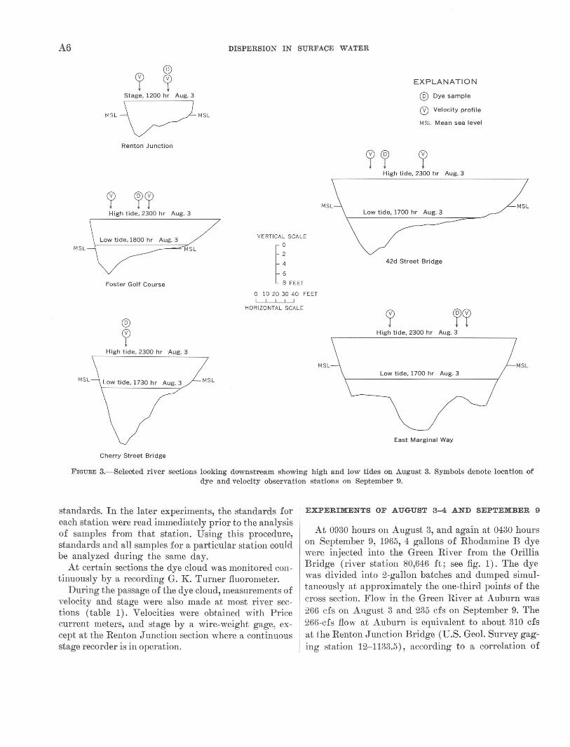


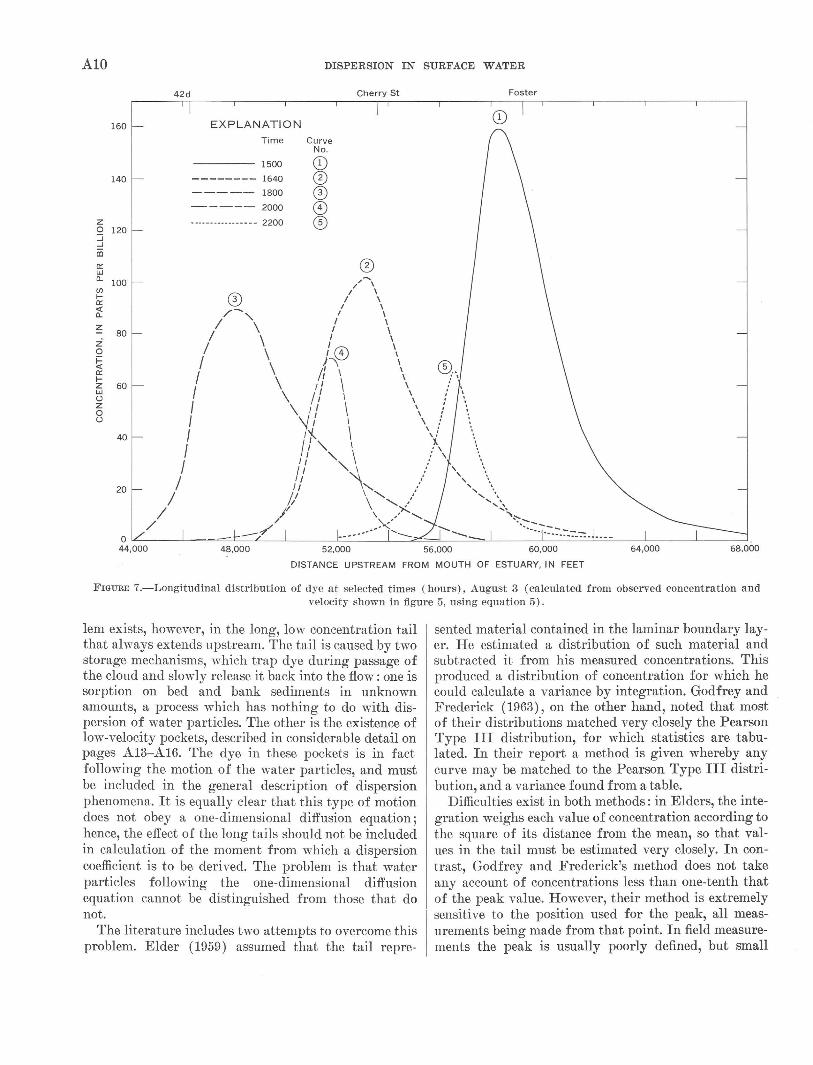

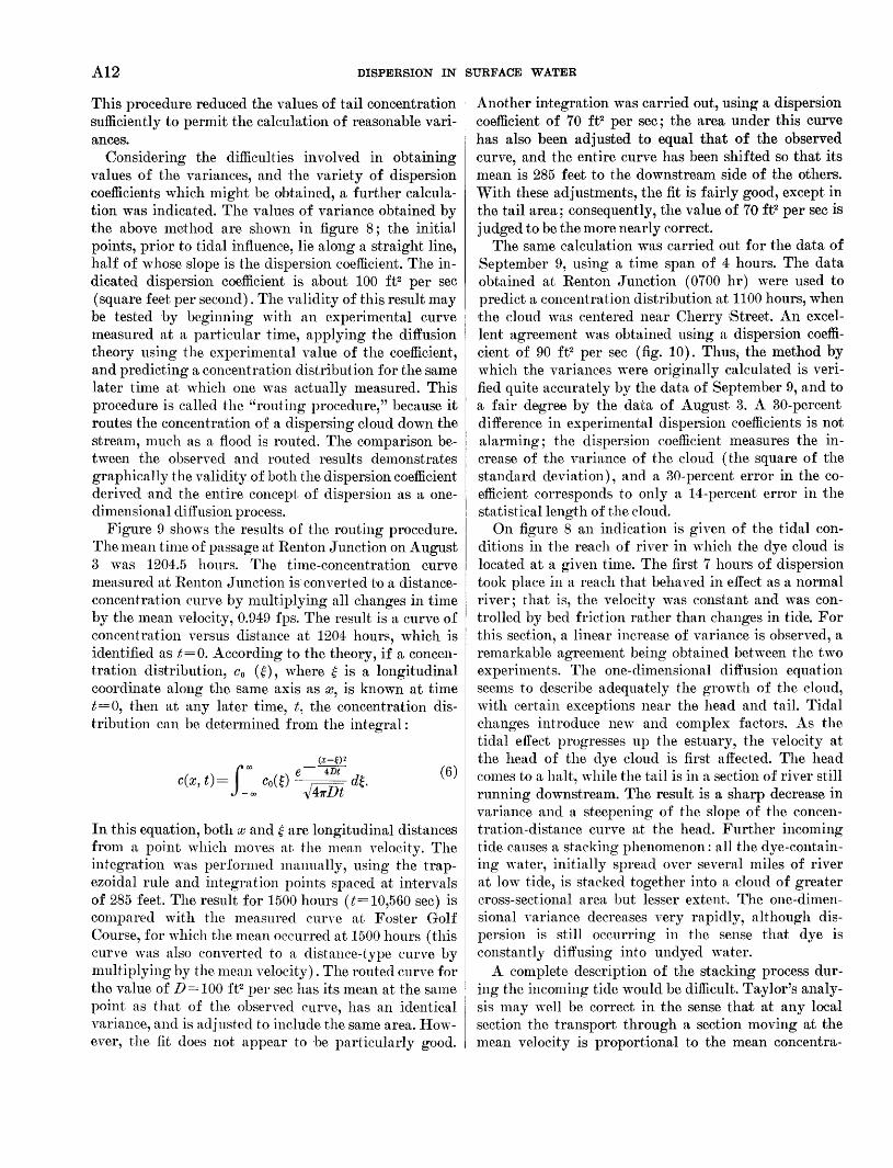

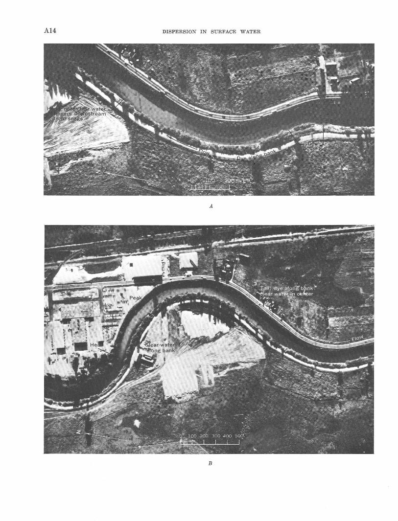
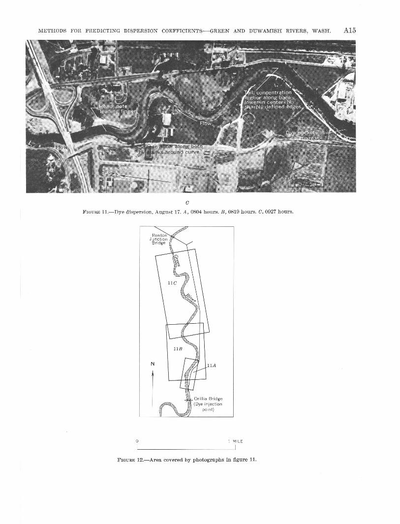
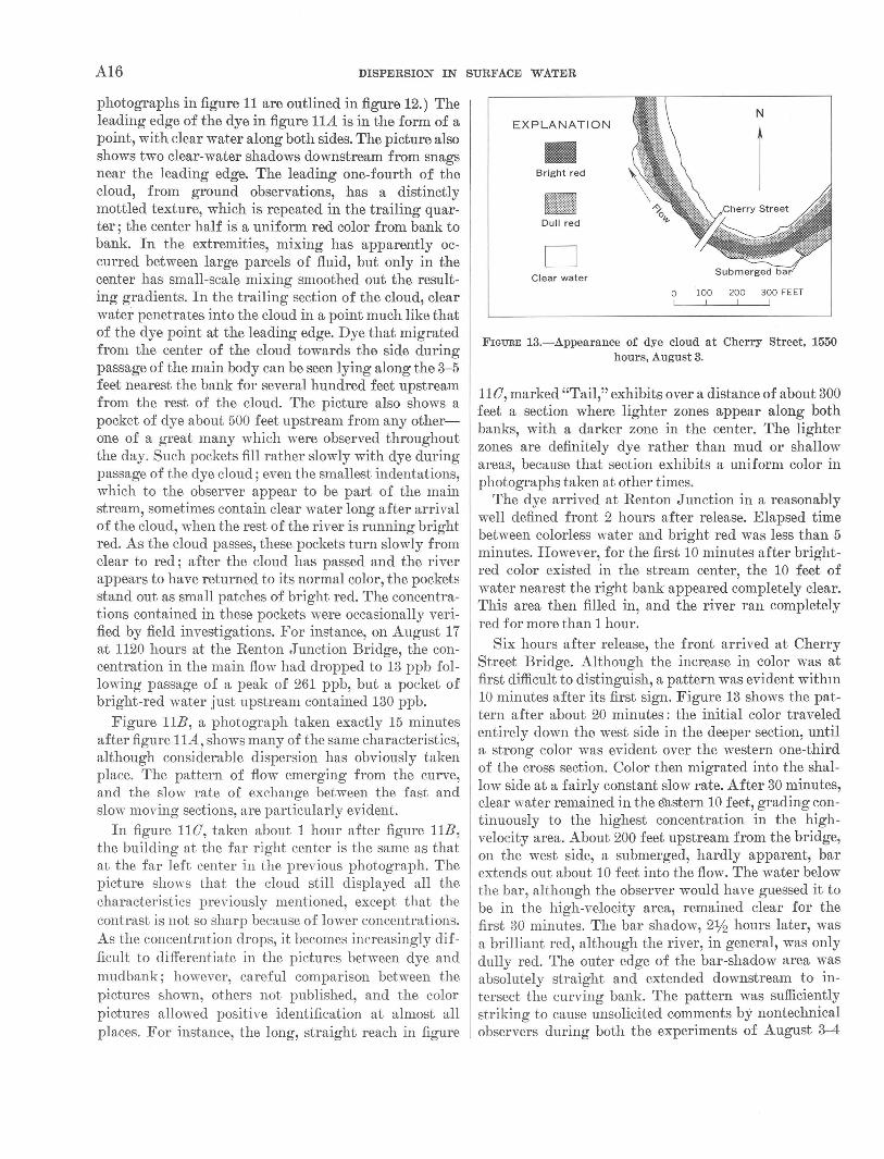
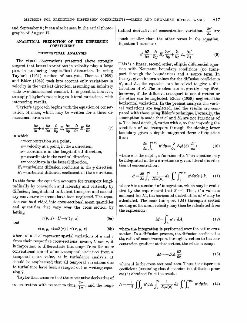
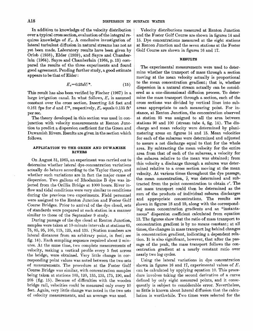

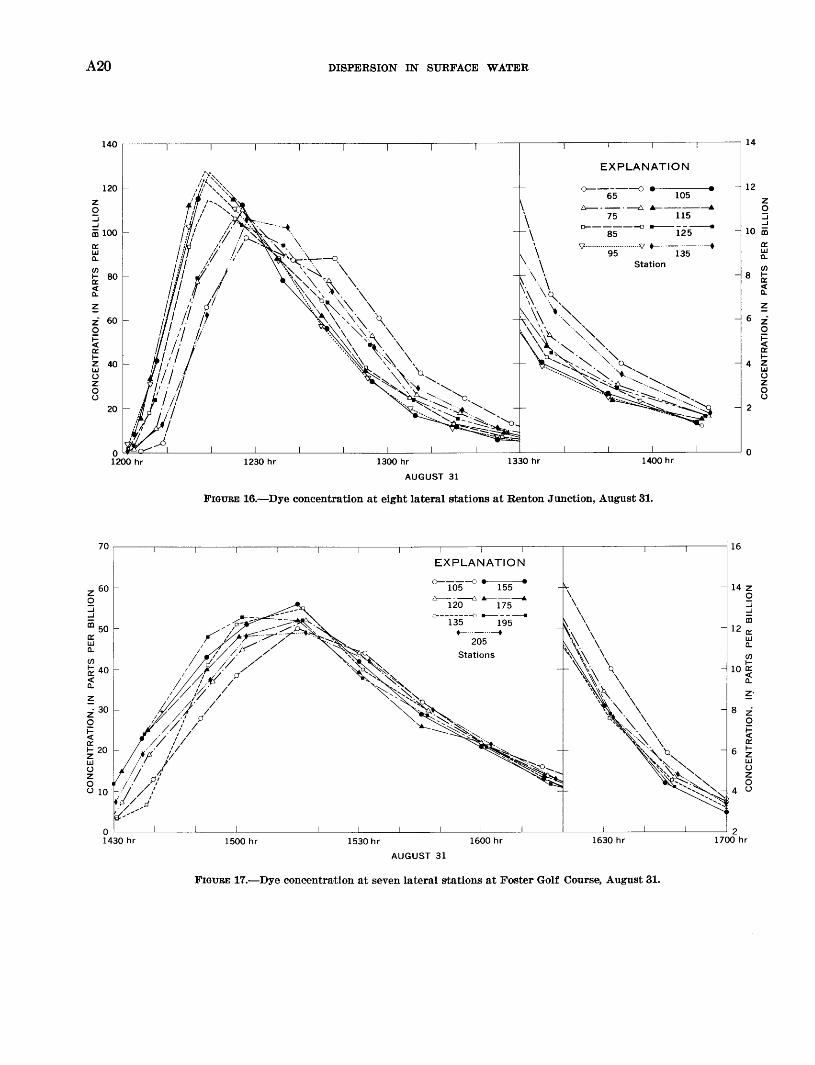


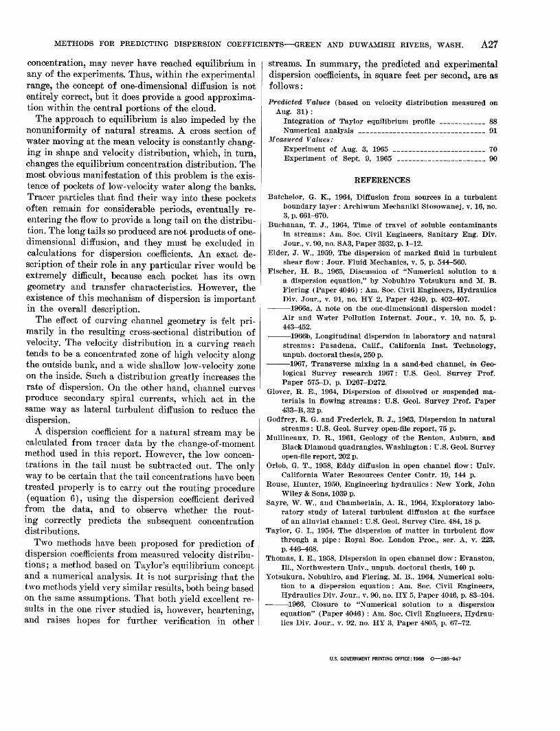


![Predicting the Coefficients of the Daubert and Danner ... · -liquid equilibrium data for3 neural network [2]. Lashkarbolooki et al. also studied the phase equilibrium for prediction](https://static.documents.pub/doc/80x56/60b4a72d7ec9236416285b32/predicting-the-coefficients-of-the-daubert-and-danner-liquid-equilibrium-data.jpg)


