Copyright 2009, The Johns Hopkins University and Saifuddin Ahmed. All rights reserved. Use of these materials permitted only in accordance with license rights granted. Materials provided “AS IS”; no representations or warranties provided. User assumes all responsibility for use, and all liability related thereto, and must independently review all materials for accuracy and efficacy. May contain materials owned by others. User is responsible for obtaining permissions for use from third parties as needed. This work is licensed under a Creative Commons Attribution-NonCommercial-ShareAlike License . Your use of this material constitutes acceptance of that license and the conditions of use of materials on this site.
Transcript
Copyright 2009, The Johns Hopkins University and Saifuddin Ahmed. All rights reserved. Use of these materials permitted only in accordance with license rights granted. Materials provided “AS IS”; no representations or warranties provided. User assumes all responsibility for use, and all liability related thereto, and must independently review all materials for accuracy and efficacy. May contain materials owned by others. User is responsible for obtaining permissions for use from third parties as needed.
This work is licensed under a Creative Commons Attribution-NonCommercial-ShareAlike License. Your use of this material constitutes acceptance of that license and the conditions of use of materials on this site.
In stratified sampling the population is partitioned into groups, called strata,
and sampling is performed separately within each stratum.
When?• Population groups may have different values
for the responses of interest.
• If we want to improve our estimation for each group separately.
• To ensure adequate sample size for each group.
In stratified sampling designs:
• stratum variables are mutually exclusive (non-over lapping), e.g., urban/rural areas, economic categories, geographic regions, race, sex, etc.
• the population (elements) should be homogenous within-stratum, and
• the population (elements) should be heterogenous between the strata.
Advantages• Provides opportunity to study the stratum
variations - estimation could be made for each stratum
• Disproportionate sample may be selected from each stratum
• The precision likely to increase as variance may be smaller than SRS with same sample size
• Field works can be organized using the strata (e.g., by geographical areas or regions)
• Reduce survey costs.
The principal objective of stratification is to reduce
sampling errors.
Disadvantages
• Sampling frame is needed for each stratum• Analysis method is complex
– Correct variance estimation• Data analysis should take sampling “weight”
into account for disproportionate sampling of strata
• Sample size estimation is difficult in practice
When sample is selected by SRS technique independently within
each stratum, the design is called stratified random sampling.
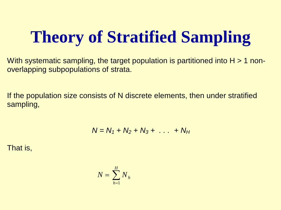
Theory of Stratified SamplingWith systematic sampling, the target population is partitioned into H > 1 non-overlapping subpopulations of strata. If the population size consists of N discrete elements, then under stratified sampling, N = N1 + N2 + N3 + . . . + NH That is,
∑=
=H
hhNN
1
Estimation of Total for a random variable y
Let yhi = value of ith unit in stratum h Then, population total for stratum h is:
And, population total is:
That is, t = t1 + t2 + t3 + . . . + tH (compare to: N = N1 + N2 + N3 + . . . + NH )
∑=
=hN
ihih yt
1
∑=
=H
hhtt
1
Strata totals are additive But, not the strata means
Population mean for strata h is:
However,
Because,
Strata means are not additive
h
hh N
ty =
Hyyyy +++≠ ....21
H
H
H
H
Nt
Nt
Nt
NNNttt
Nt
y +++≠++++++
== .........
2
2
1
1
21
21
However, we can formulate an additive relationship, by “weight” factors:
Where,
Note that,
HH yWyWyWy +++= ....2211
NN
W hh =
11
=∑=
H
hhW
Proof:
Nt
Nt
Nt
Nt
yN
Ny
NN
yNN
yN
Ny
NN
yNN
yWyWyWy
H
HH
HH
HH
=
+++=
+++=
+++=
+++=
....
....
....
....
21
22
11
22
11
2211
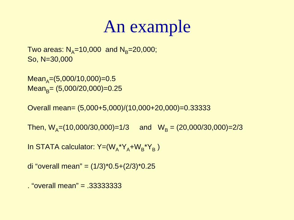
An exampleTwo areas: NA =10,000 and NB =20,000; So, N=30,000
• When the elements are homogenous (quite similar), there is less variance [variance(within) is smaller]
• Because variance(between strata)=0 in stratified sampling design, smaller the variance(within), smaller the total(variance).
variance(total) = variance(within) + 0
So, the objective is to increase variance(between) and decrease variance(within).
Sample Size Estimation for Stratified Sampling Design
• Sample size estimation for stratified sampling is difficult in practice, not for the complexity of sample size formula.
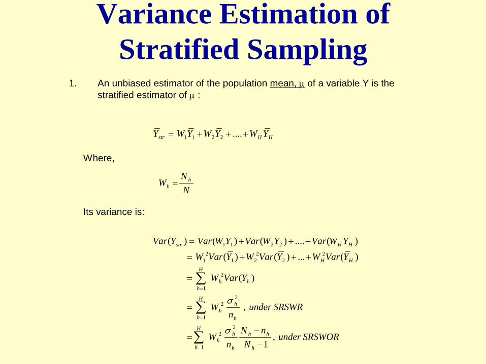
• Sample size estimation depends on variance estimation. Consider the variance of a mean for a variable y:
h
hh
h
hH
h
h
hh
h
hhH
h
h
hh
h
hhH
h
hh
strstr
NnN
nsW
NnN
ns
NN
SRSWORunderN
nNns
NN
tVarN
NtVaryraV
−=
−⎟⎠⎞
⎜⎝⎛=
−=
=
⎟⎠
⎞⎜⎝
⎛=
∑
∑
∑
∑
=
=
=
=
22
1
22
1
2
2
2
1
12
,
)ˆ(1
ˆ)(ˆ
Under SRS[WR]
Problem• The variance
estimation, even under “with replacement,” needs information on additional three factors: N, Nh , s2
h .
• It is very difficult or impossible to get information on s2
h from each stratum.
h
hh
h
hH
h
h
hh
h
hhH
h
h
hh
h
hhH
h
hh
strstr
NnN
nsW
NnN
ns
NN
SRSWORunderN
nNns
NN
tVarN
NtVaryraV
−=
−⎟⎠⎞
⎜⎝⎛=
−=
=
⎟⎠
⎞⎜⎝
⎛=
∑
∑
∑
∑
=
=
=
=
22
1
22
1
2
2
2
1
12
,
)ˆ(1
ˆ)(ˆ
Sample Size Estimation for Stratified Sampling Design
• For those want to try!
• Substitute ph (1-ph ) for binary outcomes (proportions).
• In practice, stratified sampling SS estimation is done under SRS assumption (more conservative) or preferably multi-stage sampling design method is used, and not done as a single stage sampling strategy.
∑
∑
=
=
+⎟⎟⎠
⎞⎜⎜⎝
⎛=
H
hhh
H
h h
hh
SNZ
dN
nnSN
n
1
2
2/2
22
1
22
)/(
α
Allocation of Stratified Sampling
The major task of stratified sampling design is the
appropriate allocation of samples to different strata .Types of allocation methods:• Equal allocation• Proportional to stratum size• Allocation based on variance differences
among the strata• Cost based sample allocation
Equal Allocation• Divide the number of sample units n equally
among the K strata.
• Formula: nh = n/K
• Example: n = 100; 4 strata; sample nh =100/4 = 25 in each stratum.
• May not be equal in each stratum. (what if you have 3 strata?)
• Need “weighted analysis” (disproportionate selection)
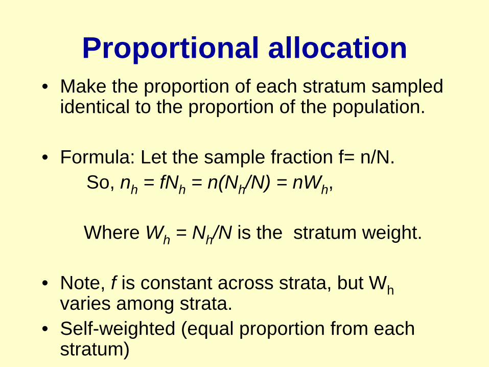
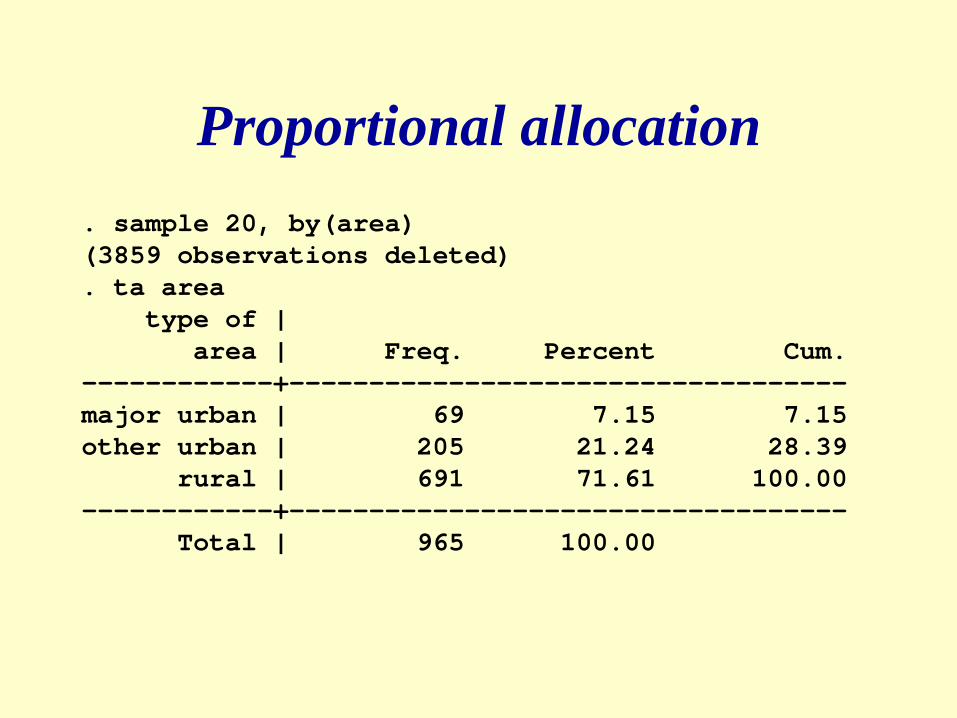
Proportional allocation• Make the proportion of each stratum sampled
identical to the proportion of the population.
• Formula: Let the sample fraction f= n/N. So, nh = fNh = n(Nh /N) = nWh ,
Where Wh = Nh /N is the stratum weight.
• Note, f is constant across strata, but Wh varies among strata.
• Self-weighted (equal proportion from each stratum)
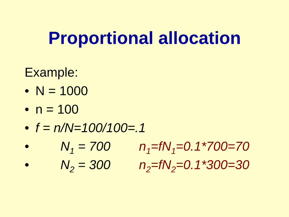
Proportional allocation
Example:• N = 1000 • n = 100• f = n/N=100/100=.1• N1 = 700 n1 =fN1 =0.1*700=70• N2 = 300 n2 =fN2 =0.1*300=30
Disadvantages
• A major disadvantage of proportional allocation:– Sample size in a stratum may be low – provide
unreliable stratum-specific results.• A major disadvantages of equal allocation:
– May need to use weighting to have unbiased estimates.
Optimal allocation (Neyman Allocation)
Based on the variability of sampling: more variable strata should be sampled more intensely.
Formula:
• Need “weighted analysis” (disproportionate selection)
SS may not be adequate for stratum specific analysis
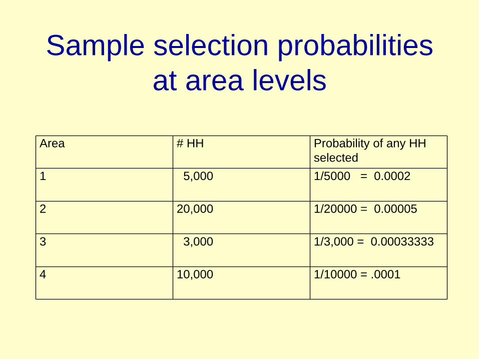
Probability Proportional to Size (PPS)
• PPS is very common in large surveys. • In simplistic sense, the selection probability
that a particular sampling unit will be selected in the sample is proportional to the size of the variable of interest (e.g., in a population survey, the population size of the sampling unit).
• PPS sampling provides self-weighted samples.
Sample selection probabilities at area levels
Area # HH Probability of any HH selected
1 5,000 1/5000 = 0.0002
2 20,000 1/20000 = 0.00005
3 3,000 1/3,000 = 0.00033333
4 10,000 1/10000 = .0001
Use of PPS
• when the populations of the sampling units vary, and
• to ensure that every element in the target population has an equal chance of being included in the sample (self weighted).
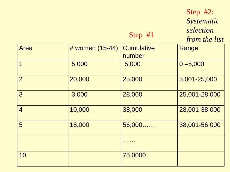
Steps in PPS Sampling:
• Creating a list of clusters with cumulative population size
• Selecting a systematic sample from a random start using a sampling interval,
• Please see the handout for an example
Area # women (15-44) Cumulative number
Range
1 5,000 5,000 0 –5,000
2 20,000 25,000 5,001-25,000
3 3,000 28,000 25,001-28,000
4 10,000 38,000 28,001-38,000
5 18,000 56,000…… 38,001-56,000
……
10 75,0000
Step #1
Step #2:Systematic selection from the list
Some practical considerations
• Conceptually, quite similar to systematic sampling
• PPS is very attractive in practice because no weighting is required
• However, due to other reasons (missing responses), weighting may not be avoided.