Metocean Study Pituffik Greenland - Dundas

1856/U16424/B/BvL November 18th 2016

Metocean Study Pituffik Greenland

Analysis of Ice, Winds, Currents and Waves

Final

Document title Metocean Study Pituffik Greenland

Analysis of Ice, Winds, Currents and Waves

Short document title Metocean Study Pituffik

Status Final

Date November 18th

2016

Project name Metocean Study Pituffik

Project number 1856

Client IHC Mining

Reference 1856/U16424/B/BvL

Author Ype Attema and Bas van Leeuwen

Checked by Lynyrd de Wit

Disclaimer

The services provided by Svašek Hydraulics in this report are based upon meteorological and oceanographic

analyses. Such analyses are of a predictive nature and, as a result, contain elements of uncertainty for which

no assurance can be given. Therefore, it is agreed that Svašek Hydraulics shall have no liability for any

damages arising out of or caused by actions or forces of nature whether or not these were predicted and/or

addressed in a non predictive way by Svašek Hydraulics.

Schiehaven 13G

3024 EC Rotterdam

The Netherlands

T +31 - 10 - 467 13 61

F +31 - 10 - 467 45 59

E [email protected]

I www.svasek.com

Metocean Study Pituffik 1856/U16424/B/BvL

Final -1- November 18th 2016

TABLE OF CONTENTS

Pag.

1 INTRODUCTION 3

2 ICE AND OPEN WATER 4 2.1 Introduction 4 2.2 Regional analysis of Satellite based Ice Coverage maps 4 2.3 Local analysis based on Satellite images 9 2.4 Conclusions 10

3 WINDS 11 3.1 Verification of long term global wind data 11 3.2 Local winds in 'inlet' 15 3.3 Extreme and operational wind conditions 17

4 CURRENTS AND TIDES 19 4.1 Modelling Software 19 4.2 Model setup 19 4.2.1 Computational grid 19 4.2.2 Bathymetry 20 4.2.3 Astronomical boundary conditions 21 4.2.4 Meteorological conditions 21 4.2.5 Ice conditions 21 4.3 Model validation 22 4.4 Results Hydrodynamic FINEL2D simulations 24 4.4.1 Modelled water level variations 24 4.4.2 Modelled current velocity 24

5 WAVES 27 5.1 General approach 27 5.2 'Offshore' SWAN model of northern Baffin Bay and southern Nares

Strait 27 5.2.1 Domain, computational grid and bathymetry 27 5.2.2 Spectral and directional bins 30 5.2.3 Enforced winds and simulation of ice cover 30 5.2.4 Results 30 5.3 Small scale 'inlet' model 32 5.3.1 Domain, computational grid and bathymetry 32 5.3.2 Spectral and directional bins 33 5.3.3 Ice cover 33 5.3.4 Enforced winds 33 5.3.5 Results 33 5.4 Combining time series and determining extreme and operational

conditions 35 5.5 Extreme and wave conditions 37



6 SUMMARY 40

7 RECOMMENDATIONS 41

REFERENCES 42



1 INTRODUCTION

The study before you concerns metocean conditions (ice, winds, currents and wave) for Pituffik, Greenland, see Figure 1.1. This report will provide the design and operational conditions for a scoping level feasibility study of an ilmenite mining operation in the coastal zone conducted by IHC Mining who in turn are contracted by FinnAust Mining.

Figure 1.1: Area of interest between Boffin Bay (South) and Nares Strait (North). Baffin Bay is connected to the Atlantic Ocean to the south. Image source: Universität Tübingen.

In consultation with the client four output locations have been selected, see figure below. The 15 m contour gives an idea of near shore conditions without going into complicated beach processes (wave breaking, wave generated long shore currents), which fall outside of the scope of this study. Currents and waves will be specified for these four locations. For ice, winds, and water levels there is no meaningful distinction to be made for locations so close together, for these cases one central output location is employed.

Figure 1.2: Output locations for current and wave conditions.

This report starts with an ice and open water analysis, followed by the derivation of wind data. Both of these form input for the tidal and wave simulations in the two chapters that follow.



2 ICE AND OPEN WATER

2.1 Introduction

An ice analysis has been made to determine the open water season for the project.

A distinction is made between a local analysis based on satellite imagery and a regional assessment

of ice charts of Baffin Bay and the connection to the Atlantic Ocean. It appears that the project

location is ice free before the connection to the Atlantic Ocean is open. If both were necessary for

operations (which is not yet certain at this point in time) the latter would be the critical factor.

2.2 Regional analysis of satellite based ice coverage maps

A 12 year database (2004-present) with a 12 km resolution in the area of interest has been obtained

(NCEP MMAB 12km). A more expansive series is also available, but for years before 2004 the

resolution decreases to 24 km. Only the high resolution fields are used in this analysis. The database

contains daily ice fields which give ice coverage for each grid element between 0 (no ice) and 1 (full

coverage).

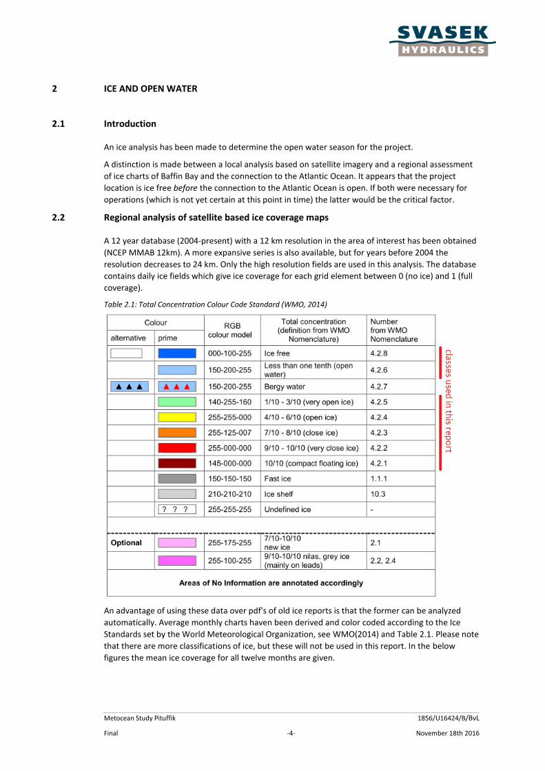
Table 2.1: Total Concentration Colour Code Standard (WMO, 2014)

An advantage of using these data over pdf's of old ice reports is that the former can be analyzed

automatically. Average monthly charts haven been derived and color coded according to the Ice

Standards set by the World Meteorological Organization, see WMO(2014) and Table 2.1. Please note

that there are more classifications of ice, but these will not be used in this report. In the below

figures the mean ice coverage for all twelve months are given.



Please note that most coastal locations are never ice free in the images. This is clearly unrealistic and

probably due to an interpolation error in the algorithm used to derive the maps. This means that the

ice coverage charts can only be used for open sea areas and not for coastal zones.

Figure 2.1: Mean ice coverage, January to April. Area of interest is given by a square.



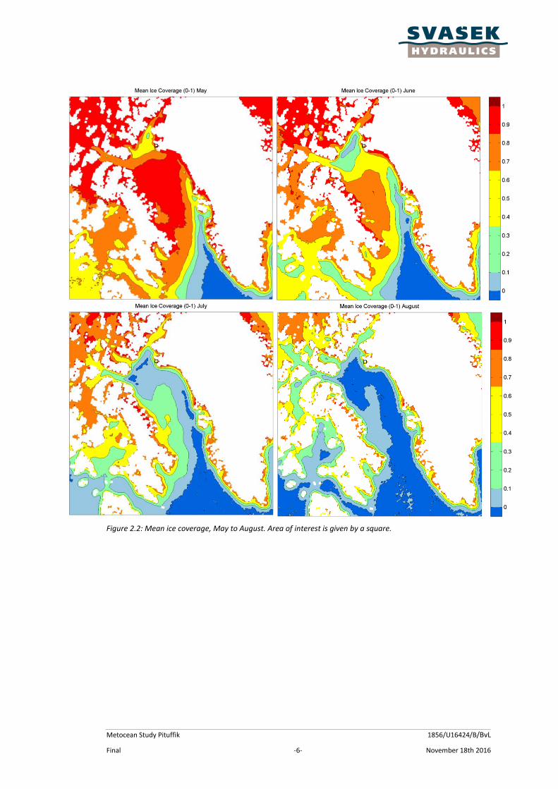
Figure 2.2: Mean ice coverage, May to August. Area of interest is given by a square.



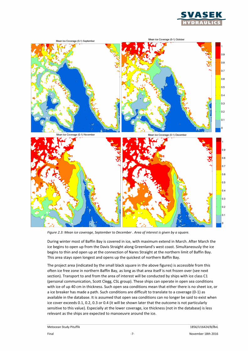
Figure 2.3: Mean ice coverage, September to December . Area of interest is given by a square.

During winter most of Baffin Bay is covered in ice, with maximum extend in March. After March the

ice begins to open up from the Davis Straight along Greenland's west coast. Simultaneously the ice

begins to thin and open up at the connection of Nares Straight at the northern limit of Baffin Bay.

This area stays open longest and opens up the quickest of northern Baffin Bay.

The project area (indicated by the small black square in the above figures) is accessible from this

often ice free zone in northern Baffin Bay, as long as that area itself is not frozen over (see next

section). Transport to and from the area of interest will be conducted by ships with ice class C1

(personal communication, Scott Clegg, CSL group). These ships can operate in open sea conditions

with ice of up 40 cm in thickness. Such open sea conditions mean that either there is no sheet ice, or

a ice breaker has made a path. Such conditions are difficult to translate to a coverage (0-1) as

available in the database. It is assumed that open sea conditions can no longer be said to exist when

ice cover exceeds 0.1, 0.2, 0.3 or 0.4 (it will be shown later that the outcome is not particularly

sensitive to this value). Especially at the lower coverage, ice thickness (not in the database) is less

relevant as the ships are expected to manoeuvre around the ice.



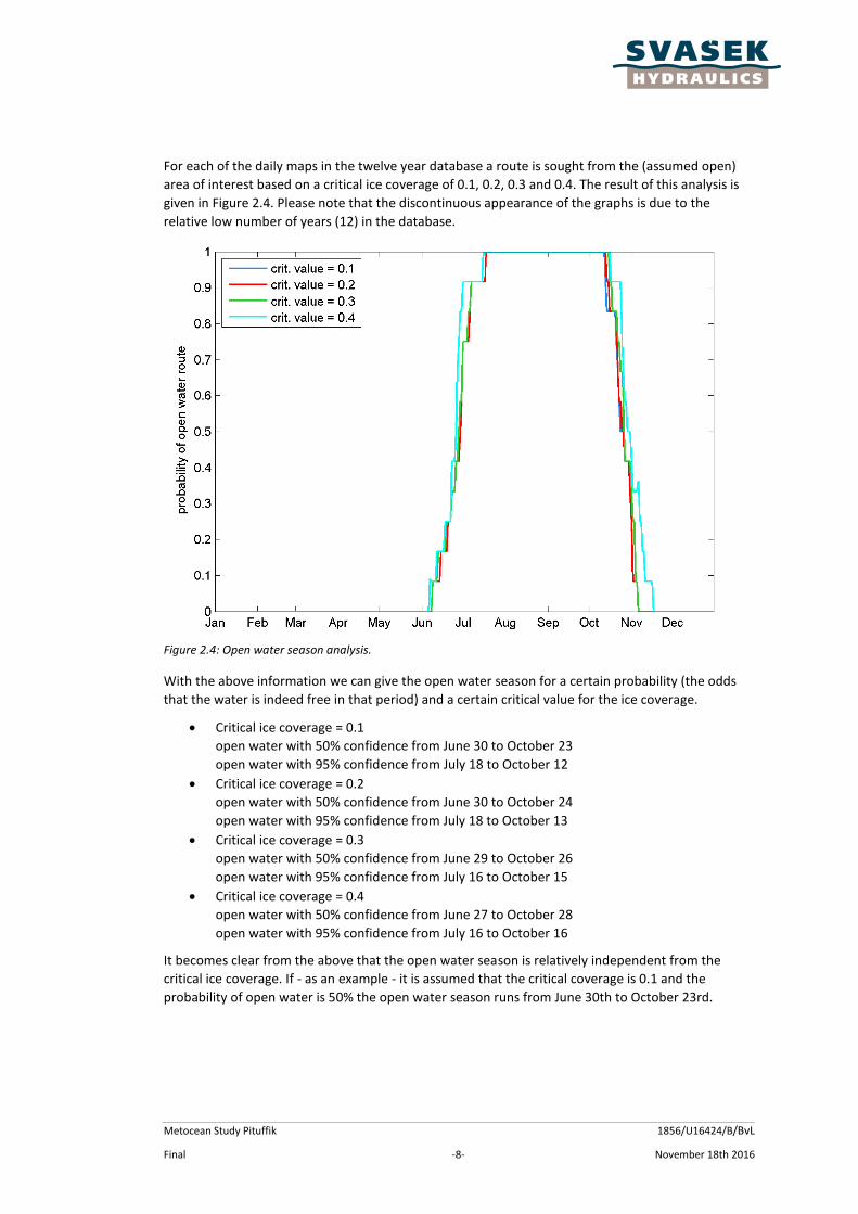
For each of the daily maps in the twelve year database a route is sought from the (assumed open)

area of interest based on a critical ice coverage of 0.1, 0.2, 0.3 and 0.4. The result of this analysis is

given in Figure 2.4. Please note that the discontinuous appearance of the graphs is due to the

relative low number of years (12) in the database.

Figure 2.4: Open water season analysis.

With the above information we can give the open water season for a certain probability (the odds

that the water is indeed free in that period) and a certain critical value for the ice coverage.

Critical ice coverage = 0.1

open water with 50% confidence from June 30 to October 23

open water with 95% confidence from July 18 to October 12










It becomes clear from the above that the open water season is relatively independent from the

critical ice coverage. If - as an example - it is assumed that the critical coverage is 0.1 and the

probability of open water is 50% the open water season runs from June 30th to October 23rd.



2.3 Local analysis based on satellite images

The previous section has given the accessibility of the area of interest from the Atlantic Ocean. To be

answered is the question whether the project location itself is accessible. Ice charts do not have the

detail necessary or are unreliable in the coastal zone. What is left is to look at actual satellite images

of the area of interest.

The Danish Meteorological Institute (see http://ocean.dmi.dk/arctic/qaanaaq.uk.php) gives a good

overview of the available images for the Greenland coastline. A thorough analysis of these images

goes beyond the scope of the current project, however a quick scan has been made of the images of

the Aqua satellite of the past three springs. The following conclusions can be made:

Project location ice free:

- 2016, April 29th (see Figure 2.5)

- 2015, May 20th.

- 2014, April 16th.

Figure 2.5: Aqua satellite image (April 29th 2016, source: website DMI). Project area in orange circle.

In general it can be said that if the Nares Straight is ice free, the project location will be as well. As

can be seen in Figure 2.2 this is usually the case from June onward, with the ice opening up in April

and May.

This being said, there are numerous occasions when significant amounts of ice block the project

location well into June (see Figure 2.6). It is questionable whether conditions such as these can be

considered 'workable'. This ice breaks away from sheets still present in Baffin Bay well into summer.

Residual density driven (3D) currents bring this ice northward. A more extensive analysis, based on -

in advance agreed upon - criteria may be advisable in this regard. A more in depth review of freely

available satellite images would be a part of this analysis.



Figure 2.6: Aqua satellite image (June 13th 2014, source: website DMI). Project area in orange circle.

The start of the open water season (around April - July) has lots of sun light for satellite photographs.

The end of the season falls in October-November, when the sun light is very limited. Most satellite's

images are not available for this period and the ones that are, are difficult to make out. A similar

analysis to the above is thus difficult to make for the end of the season. The project location is open

up till the moment that most satellites stop giving data (October, 2015).

2.4 Conclusions

The project location is accessible (50% probability, coming from the Atlantic) from late June to late

October.

It seems that the project location itself is free of ice for at least the same period. A sampling of

satellite images (Aqua) show that the area of interest actually becomes open in April or May. After

that time significant amounts of ice can still be seen on occasions (well into June), but there is no

longer a sheet of ice covering the area. A more extensive workability analysis, based on - in advance

agreed upon - criteria may be advisable in this regard.



3 WINDS

Winds are a subject of this metocean study in the sense that operational and extreme wind

conditions are to be derived. However wind conditions are also a very important boundary

conditions in the wave simulation (Chapter 5) and to a lesser extent in the tide and current

simulation (Chapter 4).

Therefore the goal of this chapter is twofold:

Validation of long term spatially varying wind fields, to be applied in wave and current

simulations.

Derivation of wind condition at project locations and derivation of operational and extreme

conditions.

3.1 Verification of long term global wind data

Long term wind fields are obtained from the CSFR (1979-2010, Climate Forecast System Reanalysis)

database. The reanalysis has been conducted and made available by NCEP (National Centers for

Environmental Prediction), part of NOAA (National Oceanic and Atmospheric Administration). The

reanalysis consist of a combinations of models, for each cycle first a atmospheric simulation is run,

followed by an oceanic simulation. Only with those inputs a GFS (Global Forecast System) simulation

is performed which yields the winds and pressure fields used in this study. For a more in depth

explanation please see Saha et al. (2010).

Two different sources from the same model are used in this study, these data are virtually the same.

Pressure and wind fields directly from the CSFR database (used 1995-2010)

Wind fields from the derived WWIII data base (used 1995-2012, excluding 2001 and 2004).

Advantage of this data base is that ice cover is already worked into the wind fields. Note

that the last two years of the meteo input for this database are obtained from the similar

CSFR2 model which covers 2010 -2016.

For comparison with recent data (October 2016) only forecast data from GFS can be used. The model

used in these forecasts (GFS) is in principle the same as the one used in the generation of the CSFR

data.

There are two sources of validation for this dataset:

Daily wind speed and direction measurements at U.S. Thule Air Force base (1997-2016)

High Resolution Deterministic Prediction System (HRDPS) Lancaster model of the Canadian

Meteorological Centre (CMC). This model only gives a forecast of next 30 hours, so only a

few days of data are available collected around the time of the writing of this report.



Figure 3.1: Elevation plot (in m relative to M.S.L.) around area of interest, black lines give 0 and 500 m elevation contours. Source UCSD (university of California San Diego) STRM30, see section 4.2.2. Red points give locations where data is available (only one CSFR grid point shown), yellow points show locations for which data will be derived in section 3.2.

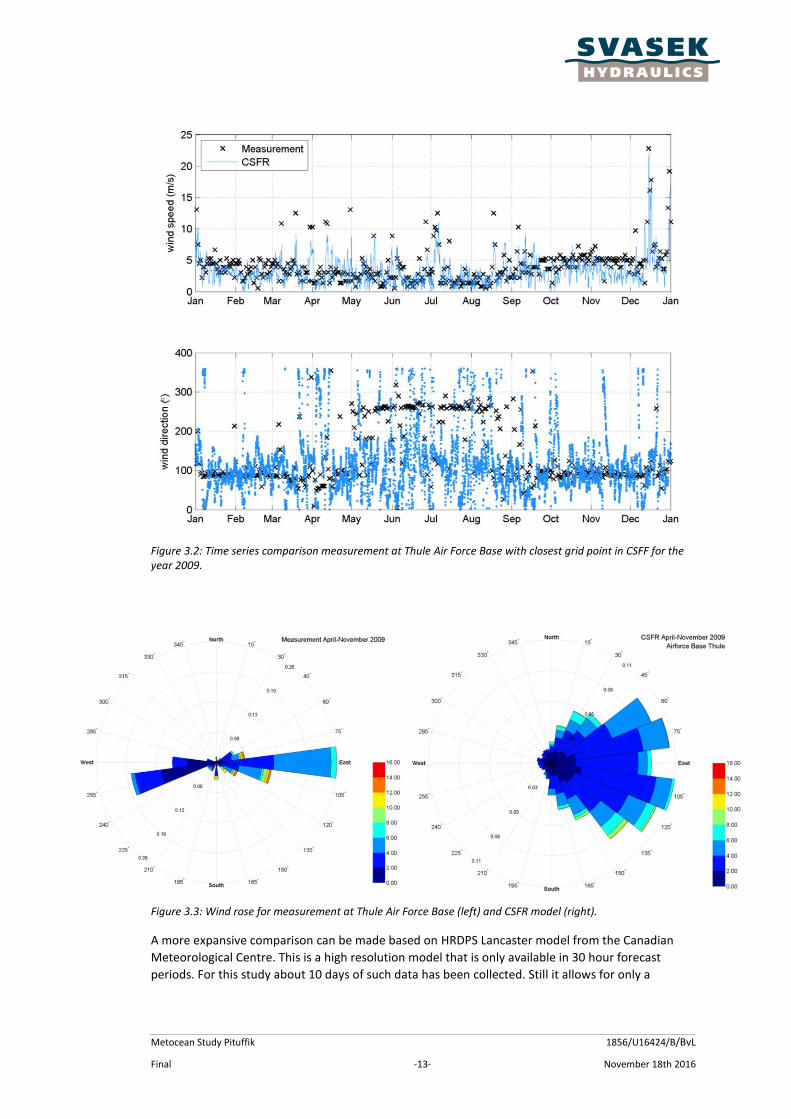
First of all, CSFR data has been extracted for 2009 for the location nearest to Thule Air Force Base

(see Figure 3.1). Please note that as CSFR has only 1/3 degree resolution, this is the closest point to

the airfield. Time series of wind speed and wind direction have been plotted in Figure 3.2. It

becomes clear that although most high wind events in the measurement series are produced well in

CSFR, the overall wind speed in the latter is too low. Also there seems to be a too high spread in the

wind directions from CSFR. Winds from the West are not present in CSFR, but it should be noted

that those winds are very weak in the measurement series as well.

The wind roses for both information sources are given in Figure 3.3. These wind roses paint the same

picture: winds are too low in CSFR, directional spread is too high and western winds are missing. It

does become clear that the eastern winds are so mild (mostly up to 2 or 4 m/s) that these are largely

irrelevant as local phenomena for wind generated waves.



Figure 3.2: Time series comparison measurement at Thule Air Force Base with closest grid point in CSFF for the year 2009.

Figure 3.3: Wind rose for measurement at Thule Air Force Base (left) and CSFR model (right).

A more expansive comparison can be made based on HRDPS Lancaster model from the Canadian

Meteorological Centre. This is a high resolution model that is only available in 30 hour forecast

periods. For this study about 10 days of such data has been collected. Still it allows for only a



snapshot comparison in time. That being said, for the data that is available the comparison does

show a consistent picture and explains the deviations between measurements and CSFR data.

As CSFR is a hindcast data base, it does not contain the recent forecast from the Lancaster model.

Instead 1/4 degree GFS forecast data have been obtained (somewhat higher resolution than GFS

output, but essentially the same model). Figure 3.4 and Figure 3.5 give the comparison between the

Lancaster model and the GFS forecasting.

Based on the entire ten day comparison series (of which only two moments have been given below

as typical examples), the following observation can be made:

Large scale wind patterns (both speed and direction) compare well between Lancaster and

GFS.

GFS does seem to underestimate wind speeds in general by about 20%.

The GFS model does miss almost entirely the small scale wind patterns which flow out of

the inlet of the area of interest. These winds are funnelled between the high hills on each

side of the inlet (see Figure 3.1) and are possibly the result from cooling and thus falling air

over glaciers.

Figure 3.4: Comparison CMC hdrps Lancaster and GFS model for October 11th 2016 18:00.

Figure 3.5: Comparison CMC hdrps Lancaster and GFS model for October 13th 2016 3:00.



3.2 Local winds in 'inlet'

From the analysis in the previous paragraph it becomes clear that Global models like GFS (and the

long time CSFR data based on it) are not capable of properly reproducing winds in the inlet between

high hills that constitutes the area of interest. This is necessary for two reasons:

Operational and extreme wind conditions are to be derived for the project location.

Eastern winds in the inlet can generate significant waves near the project locations, for

purposes of the wave study, winds in the inlet itself should be known.

The only reliable long term time series available near the output location is the measurement series

at Thule Air Force Base (1997-present). We will use the following assumptions to derive a long term

wind over the entire inlet including the project site:

Measurements at Thule Air Force Base are assumed to be correct.

There is a fixed ratio between wind velocities at the airfield on the one hand and the project

location and three fetch locations on the other (see Figure 3.1).

Ten day outputs from the Lancaster model can be used to estimate this ratio.

Wind directions in the inlet will be directed with the topography, effectively following the

coastline of the inlet. This is confirmed by the 10 day Lancaster model data.

Using the ratio from the Lancaster model, the airfield measurements can be scaled to the project

location and the three fetch locations. This method may not be entirely accurate, but it is the best

approximation for local winds based on the available data within the scope of this study.

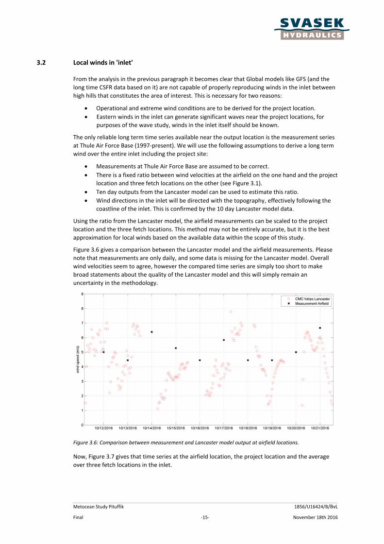
Figure 3.6 gives a comparison between the Lancaster model and the airfield measurements. Please

note that measurements are only daily, and some data is missing for the Lancaster model. Overall

wind velocities seem to agree, however the compared time series are simply too short to make

broad statements about the quality of the Lancaster model and this will simply remain an

uncertainty in the methodology.

Figure 3.6: Comparison between measurement and Lancaster model output at airfield locations.

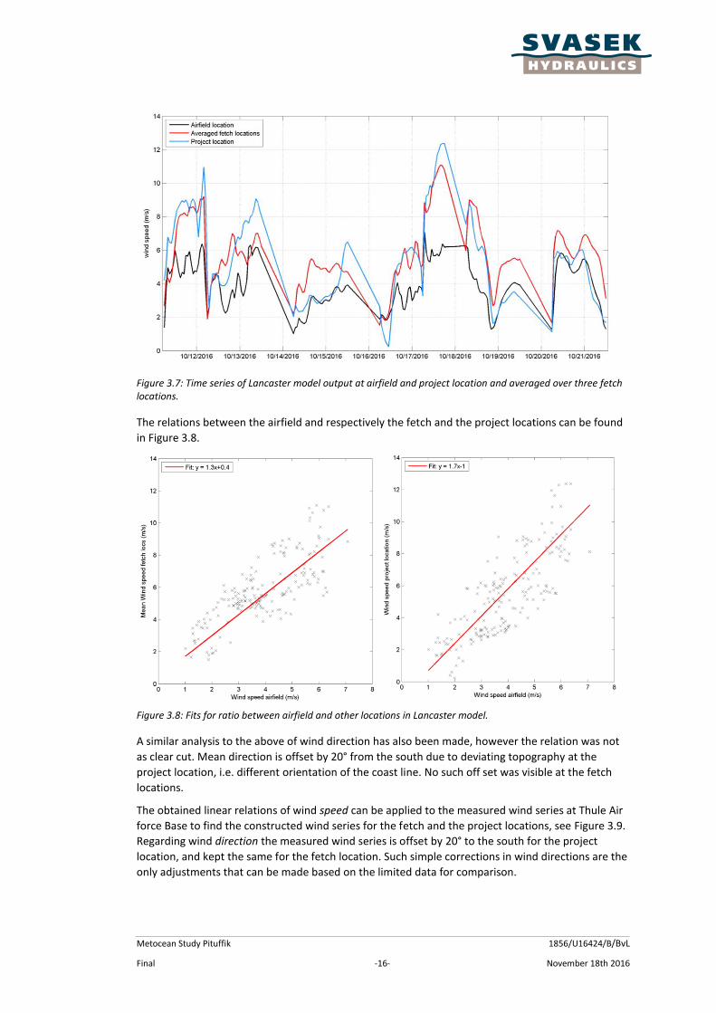
Now, Figure 3.7 gives that time series at the airfield location, the project location and the average

over three fetch locations in the inlet.



Figure 3.7: Time series of Lancaster model output at airfield and project location and averaged over three fetch locations.

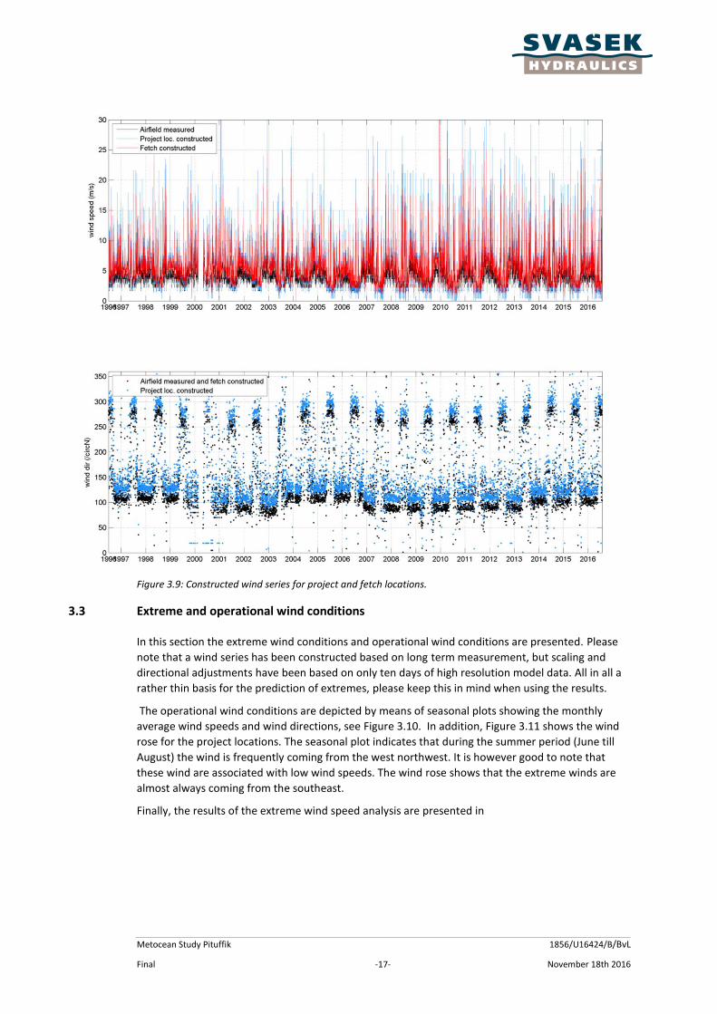
The relations between the airfield and respectively the fetch and the project locations can be found

in Figure 3.8.

Figure 3.8: Fits for ratio between airfield and other locations in Lancaster model.

A similar analysis to the above of wind direction has also been made, however the relation was not

as clear cut. Mean direction is offset by 20° from the south due to deviating topography at the

project location, i.e. different orientation of the coast line. No such off set was visible at the fetch

locations.

The obtained linear relations of wind speed can be applied to the measured wind series at Thule Air

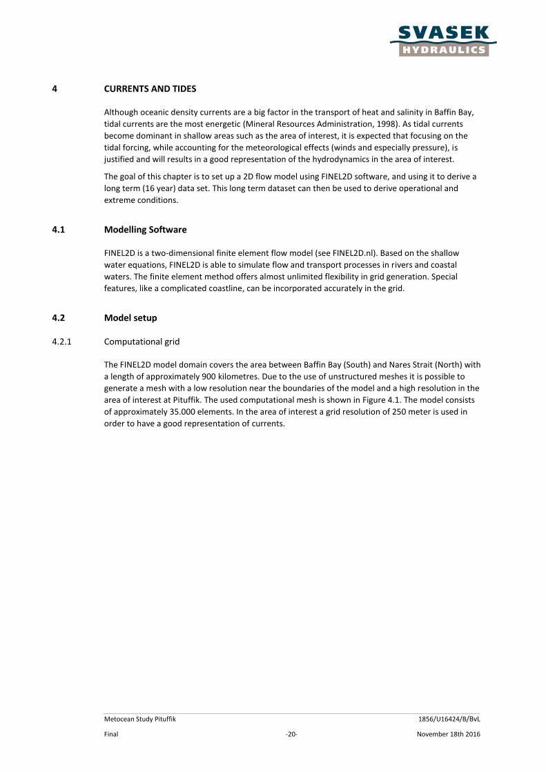
force Base to find the constructed wind series for the fetch and the project locations, see Figure 3.9.

Regarding wind direction the measured wind series is offset by 20° to the south for the project

location, and kept the same for the fetch location. Such simple corrections in wind directions are the

only adjustments that can be made based on the limited data for comparison.



Figure 3.9: Constructed wind series for project and fetch locations.

3.3 Extreme and operational wind conditions

In this section the extreme wind conditions and operational wind conditions are presented. Please

note that a wind series has been constructed based on long term measurement, but scaling and

directional adjustments have been based on only ten days of high resolution model data. All in all a

rather thin basis for the prediction of extremes, please keep this in mind when using the results.

The operational wind conditions are depicted by means of seasonal plots showing the monthly

average wind speeds and wind directions, see Figure 3.10. In addition, Figure 3.11 shows the wind

rose for the project locations. The seasonal plot indicates that during the summer period (June till

August) the wind is frequently coming from the west northwest. It is however good to note that

these wind are associated with low wind speeds. The wind rose shows that the extreme winds are

almost always coming from the southeast.

Finally, the results of the extreme wind speed analysis are presented in



Table 3.1 for return periods of 1, 10, 50 and 100 years. Based on the 25 most severe events, the

extreme wind speeds will be coming from the southeast.



Table 3.1. Extreme wind speeds for the project location.

Return period Extreme wind speed [m/s] Direction (Coming from)

1 year 25.0 Southeast

10 years 32.2 Southeast



Figure 3.10. Seasonal plot of the operational wind conditions.

Figure 3.11. Wind rose for the project location showing the wind speed and wind direction for the period April till November



4 CURRENTS AND TIDES

Although oceanic density currents are a big factor in the transport of heat and salinity in Baffin Bay,

tidal currents are the most energetic (Mineral Resources Administration, 1998). As tidal currents

become dominant in shallow areas such as the area of interest, it is expected that focusing on the

tidal forcing, while accounting for the meteorological effects (winds and especially pressure), is

justified and will results in a good representation of the hydrodynamics in the area of interest.

The goal of this chapter is to set up a 2D flow model using FINEL2D software, and using it to derive a

long term (16 year) data set. This long term dataset can then be used to derive operational and

extreme conditions.

4.1 Modelling Software

FINEL2D is a two-dimensional finite element flow model (see FINEL2D.nl). Based on the shallow

water equations, FINEL2D is able to simulate flow and transport processes in rivers and coastal

waters. The finite element method offers almost unlimited flexibility in grid generation. Special

features, like a complicated coastline, can be incorporated accurately in the grid.

4.2 Model setup

4.2.1 Computational grid

The FINEL2D model domain covers the area between Baffin Bay (South) and Nares Strait (North) with

a length of approximately 900 kilometres. Due to the use of unstructured meshes it is possible to

generate a mesh with a low resolution near the boundaries of the model and a high resolution in the

area of interest at Pituffik. The used computational mesh is shown in Figure 4.1. The model consists

of approximately 35.000 elements. In the area of interest a grid resolution of 250 meter is used in

order to have a good representation of currents.



Figure 4.1. Overview of computation mesh for FINEL2D

4.2.2 Bathymetry

The model bathymetry is compiled from two sources:

Local bathymetry survey provided by client (our Reference: 1856/ IN16491/BvL). Concerns

the coastal section, not much larger than the area covered by the four output locations.

UCSD (University of California San Diego) STRM30 data base, see Becker et al. (2009) or

refer to http://topex.ucsd.edu/WWW_html/srtm30_plus.html for more information.

Please note that a digitized navigational map was also provided by the client (our reference

1856/IN16528/BvL). This map was used to evaluate different global bathymetry sources around the

project location. UCSD STRM30 proved best in this regard and provides much more detail than the

navigational chart, so only the former was used in building up the actual model bathymetry. It should

be noted that some obvious glitches (especially anomalous shallow areas) were filtered from the

UCSD set based on the navigational map.

An overview of the bathymetry at different detail levels is depicted in Figure 4.2.



Figure 4.2.Overview of bathymetry for FINEL2D

4.2.3 Astronomical boundary conditions

The tidal water level variations in the model are driven by deepwater open boundaries. These

boundaries located on the South and the North side of the model and are forced by thirteen TPXO

(see Egbert and Erofeeva, 2002) astronomical tidal components. By applying this tidal boundary the

tidal water level variations and currents are accounted for within the model domain.

4.2.4 Meteorological conditions

The meteorological conditions applied in the model consist of global wind and atmospheric pressure

fields obtained from the NOAA CSFR hindcast dataset (see Chapter 3.1). The spatial resolution of

these wind and pressure fields applied in the model are, respectively, 1/2 and 1/3 degrees, and the

temporal resolution is one hour.

4.2.5 Ice conditions

The ice coverage is not taken into account in the hydrodynamic simulation, as the effect on the tidal

variation and the current velocities in the area of interest is expected to be negligible. This certainly

holds for the area of interest during the modelled period (April - December) when the ice coverage is

low in the area of interest. The tidal water level variation is not affected by ice coverage in adjacent

areas, as the tide moves under the ice extent and remain apparent in the relatively ice free area of

interest. Also, the effect of the atmospheric pressure remains unaffected. Only, the effect of the

wind on the water levels and current velocities can be slightly overestimated if wind is coming from



adjacent areas with significant ice coverage. This effect will however be limited as wind mainly

comes in from the land side, i.e. East or South-East, and not from the ocean side that can still be

covered with ice. Therefore, it is justified to exclude the effect of the ice coverage in the

hydrodynamic simulations.

4.3 Model validation

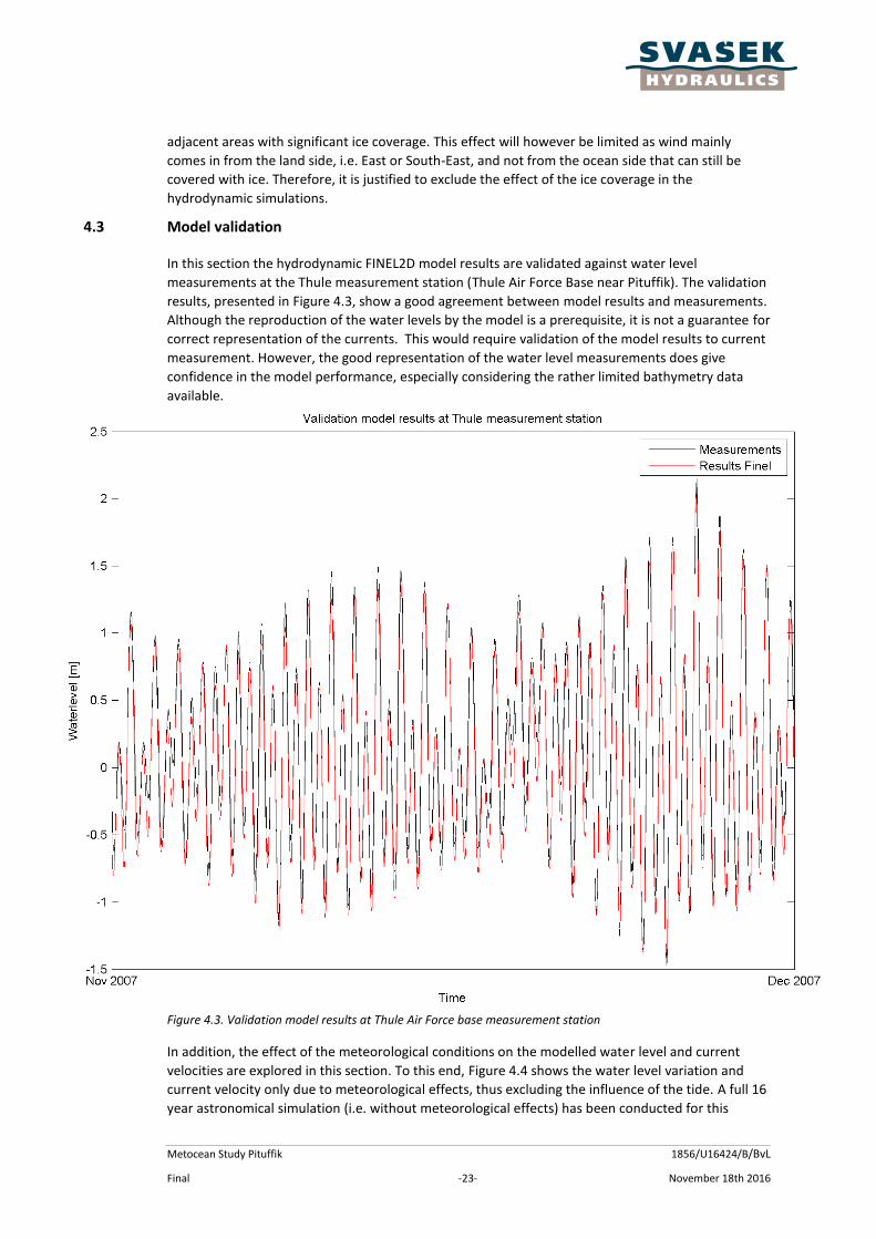
In this section the hydrodynamic FINEL2D model results are validated against water level

measurements at the Thule measurement station (Thule Air Force Base near Pituffik). The validation

results, presented in Figure 4.3, show a good agreement between model results and measurements.

Although the reproduction of the water levels by the model is a prerequisite, it is not a guarantee for

correct representation of the currents. This would require validation of the model results to current

measurement. However, the good representation of the water level measurements does give

confidence in the model performance, especially considering the rather limited bathymetry data

available.

Figure 4.3. Validation model results at Thule Air Force base measurement station

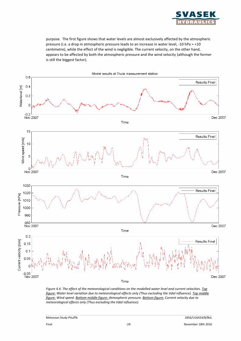
In addition, the effect of the meteorological conditions on the modelled water level and current

velocities are explored in this section. To this end, Figure 4.4 shows the water level variation and

current velocity only due to meteorological effects, thus excluding the influence of the tide. A full 16

year astronomical simulation (i.e. without meteorological effects) has been conducted for this



purpose. The first figure shows that water levels are almost exclusively affected by the atmospheric

pressure (i.e. a drop in atmospheric pressure leads to an increase in water level, -10 hPa = +10

centimetre), while the effect of the wind is negligible. The current velocity, on the other hand,

appears to be affected by both the atmospheric pressure and the wind velocity (although the former

is still the biggest factor).

Figure 4.4. The effect of the meteorological conditions on the modelled water level and current velocities. Top figure: Water level variation due to meteorological effects only (Thus excluding the tidal influence). Top middle figure: Wind speed. Bottom middle figure: Atmospheric pressure. Bottom figure: Current velocity due to meteorological effects only (Thus excluding the tidal influence).



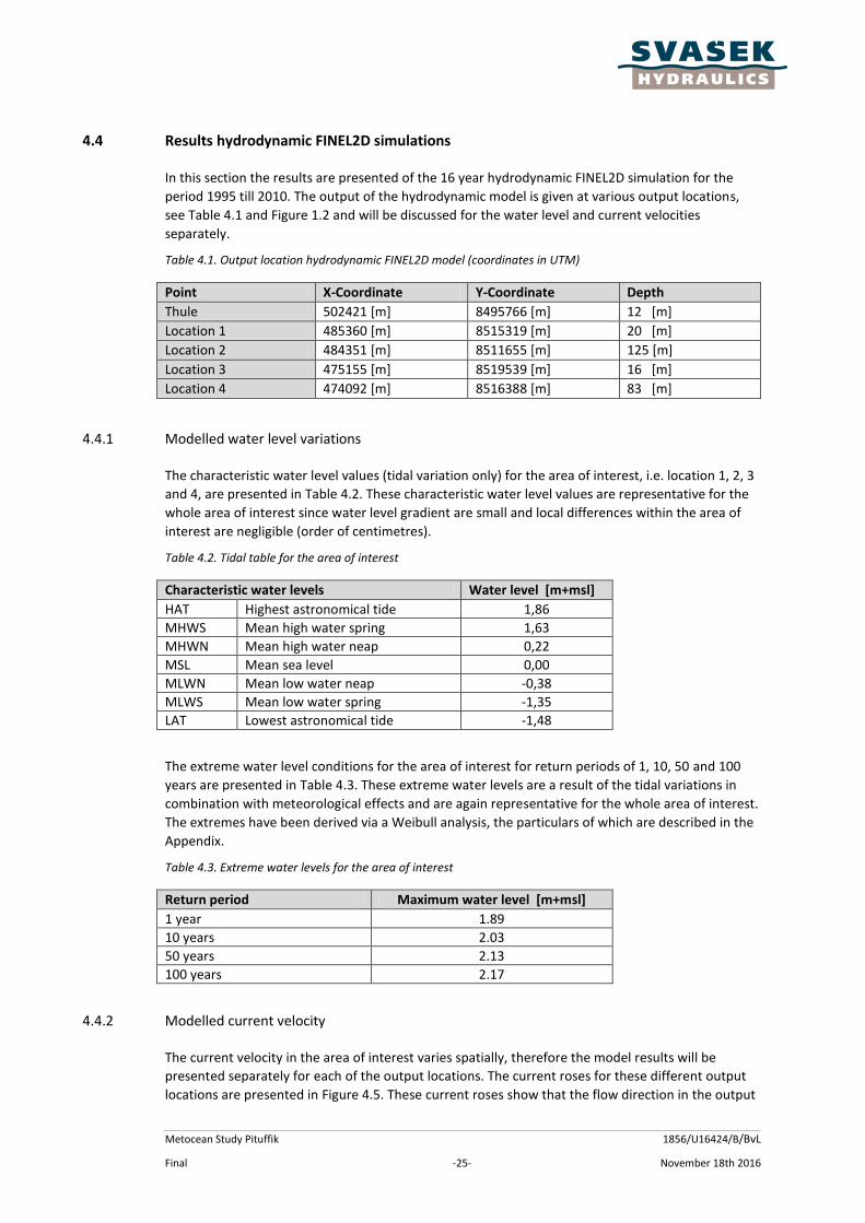
4.4 Results hydrodynamic FINEL2D simulations

In this section the results are presented of the 16 year hydrodynamic FINEL2D simulation for the

period 1995 till 2010. The output of the hydrodynamic model is given at various output locations,

see Table 4.1 and Figure 1.2 and will be discussed for the water level and current velocities

separately.

Table 4.1. Output location hydrodynamic FINEL2D model (coordinates in UTM)

Point X-Coordinate Y-Coordinate Depth

Thule 502421 [m] 8495766 [m] 12 [m]

Location 1 485360 [m] 8515319 [m] 20 [m]

Location 2 484351 [m] 8511655 [m] 125 [m]

Location 3 475155 [m] 8519539 [m] 16 [m]

Location 4 474092 [m] 8516388 [m] 83 [m]

4.4.1 Modelled water level variations

The characteristic water level values (tidal variation only) for the area of interest, i.e. location 1, 2, 3

and 4, are presented in Table 4.2. These characteristic water level values are representative for the

whole area of interest since water level gradient are small and local differences within the area of

interest are negligible (order of centimetres).

Table 4.2. Tidal table for the area of interest

Characteristic water levels Water level [m+msl]

HAT Highest astronomical tide 1,86

MHWS Mean high water spring 1,63

MHWN Mean high water neap 0,22

MSL Mean sea level 0,00

MLWN Mean low water neap -0,38

MLWS Mean low water spring -1,35

LAT Lowest astronomical tide -1,48

The extreme water level conditions for the area of interest for return periods of 1, 10, 50 and 100

years are presented in Table 4.3. These extreme water levels are a result of the tidal variations in

combination with meteorological effects and are again representative for the whole area of interest.

The extremes have been derived via a Weibull analysis, the particulars of which are described in the

Appendix.

Table 4.3. Extreme water levels for the area of interest

Return period Maximum water level [m+msl]

1 year 1.89

10 years 2.03

50 years 2.13

100 years 2.17

4.4.2 Modelled current velocity

The current velocity in the area of interest varies spatially, therefore the model results will be

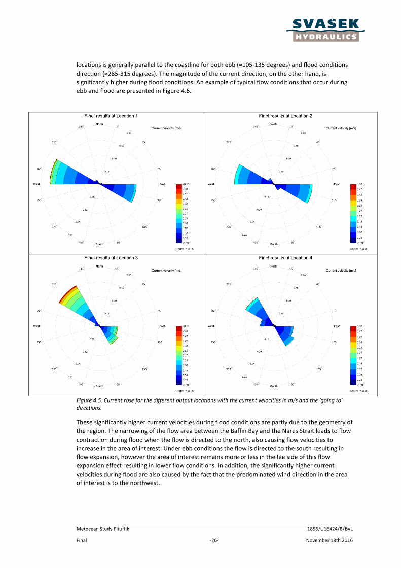
presented separately for each of the output locations. The current roses for these different output

locations are presented in Figure 4.5. These current roses show that the flow direction in the output



locations is generally parallel to the coastline for both ebb (≈105-135 degrees) and flood conditions

direction (≈285-315 degrees). The magnitude of the current direction, on the other hand, is

significantly higher during flood conditions. An example of typical flow conditions that occur during

ebb and flood are presented in Figure 4.6.

Figure 4.5. Current rose for the different output locations with the current velocities in m/s and the ‘going to’ directions.

These significantly higher current velocities during flood conditions are partly due to the geometry of

the region. The narrowing of the flow area between the Baffin Bay and the Nares Strait leads to flow

contraction during flood when the flow is directed to the north, also causing flow velocities to

increase in the area of interest. Under ebb conditions the flow is directed to the south resulting in

flow expansion, however the area of interest remains more or less in the lee side of this flow

expansion effect resulting in lower flow conditions. In addition, the significantly higher current

velocities during flood are also caused by the fact that the predominated wind direction in the area

of interest is to the northwest.



Figure 4.6. Example of current velocities patterns in the area of interest.

The extreme current velocities for the different output location for return periods of 1, 10, 50 and

100 years are presented in Table 4.4. These extreme current velocities include the effect of tidal

variation and the meteorological effects, i.e. wind and atmospheric pressure. The velocities are

expected to be significantly higher in the output locations closer to the land (location 2 and 3), which

is mainly a result of the shallower water depth at these locations. I.e. large scale flow encounters

local shallows and is accelerated over them.

Table 4.4. Extreme current velocities for the different output locations in the area of interest

Return period Location 1

Velocity [m/s]

Location 2

Velocity [m/s]

Location 3

Velocity [m/s]

Location 4

Velocity [m/s]

1 year 0.47 0.27 0.80 0.41

10 years 0.61 0.34 0.93 0.49

50 years 0.70 0.42 1.01 0.53

100 years 0.73 0.47 1.05 0.55

Mean direction

(‘Going to’) WNW WNW and ESE

1 WNW-NW WNW-NW

Please note that wave breaking on the beach itself can lead to relatively fast long shore currents not

taken into account in the flow model. A more detailed model including wave forcing would be

required. Depending on direction of incident waves this long shore current could be westward of

eastward. Please also note that, due to differences in water temperature and salinity, variations of

currents over depth (variations in both magnitude and direction) can occur at the project location

which have not been captured in the 2D hydrodynamic modelling in this study in which only the tidal

and meteorological effects (which are most energetic and thus most relevant) are taken into

account.

1 In general the extreme velocities are directed to the WNW –NW as explained earlier. For output location 2,

however, the direction of the extreme currents can either be to the WNW or to the ESE (50/50). The reason that the extreme current velocities in location 2 are also directed in the ESE is that the location is not fully in the lee side of the ebb currents anymore. Furthermore, the effect of the wind on the depth-average flow velocity is less pronounced because the output location is located in deeper water.



5 WAVES

5.1 General approach

As has been determined in section 3.1, the only available long term wind database performs

acceptably well in Baffin Bay and the Nares Strait. However those fields do not show the dominant

eastern winds in the inlet directly east of the project location. It is expected that waves generated in

Baffin Bay and the Nares Strait and waves from the inlet itself contribute to the wave climate at the

project location. Therefore both type of waves ('offshore' and 'local') will be simulated separately:

'Offshore' waves will be investigated by a large domain SWAN model based on CSFR winds,

only computing waves with a direction towards the area of interest.

'Local' waves from the inlet to the east will be investigated via a small scale 'inlet' model,

based on measurements at Thule Air Force Base.

The two resulting time series (incoming waves from offshore and local waves) will be added together

(based on energy amount). Extreme and operational conditions will be derived from this combined

series.

All waves will be computed by the wave model SWAN. SWAN is a third-generation wave model that

computes random, short-crested wind-generated waves in coastal regions and inland waters. It is

fully spectral in frequencies and directions. It is continuously being developed by Delft University of

Technology, The Netherlands.

SWAN accounts for the following relevant physical processes:

Wave generation by wind

Shoaling and refraction due to currents and depth

Three- and four-wave non-linear interactions;

White-capping, bottom friction and depth-induced breaking

Diffraction

This report uses significant wave height (Hsig), peak period (Tp) and mean wave direction (dir).

Significant wave height (in m) is originally defined as the average wave height of the third highest

waves (H1/3). In practice it is usually defined as four times the standard deviation of the surface

elevation (Hm0) which is the definition used in this report (deviates only a few percent from H1/3).

The peak wave period (in seconds) is defined as the wave period associated with the most

energetic (highest) waves in the total wave spectrum. Mean wave direction can be interpreted as the

name suggest and in a technical sense as the vectorial mean wave direction as a function of

frequency.

5.2 'Offshore' SWAN model of northern Baffin Bay and southern Nares Strait

5.2.1 Domain, computational grid and bathymetry

The area of interest cannot be reached by swell waves from for example the Atlantic ocean, the area

of interest is simply too sheltered by surrounding topography. All waves relevant for the area of

interest are thus generated in the direct vicinity or in the northern part of Baffin Bay. The domain of

the 'Offshore' model has been selected to include all these relevant fetches for wind generated

waves. Any water outside this area can be omitted from the model, hence the model boundaries in

the north, west and south. In reality waves will come into the model domain over these boundaries,

but as they can never reach the area of interest (due to topography), they can safely be ignored.



Figure 5.1: Overview of 'offshore' wave model computational grid and bathymetry, detailed view of area within red border in Figure 5.2.

Computational grid size varies between 7500 m (sides of triangles) for most of the model, to 250 m

sides in the area of interest. A finer grid size did not lead to significantly different results in the area

of interest, nor does it improve numerical performance. Bathymetry source files are equal to those

used in the current study. Some smoothing is applied for numerical reasons.



Figure 5.2: 'Offshore' wave model detail of area of interest computational grid (above) and bathymetry (below).



5.2.2 Spectral and directional bins

Wave spectra in SWAN consist of energy divided over a number of directional and spectral bins.

Spectral space runs from 0.05 to 2.00 Hz and is divided into 39 not equidistant bins (this means that

waves with periods of 0.5 to 20 second can be taken into account).

The directional space runs from 135 °N to 315 °N divided into 36 5° bins, see lower panel of Figure

5.2. This choice is made to save computational time. It also means that no waves can enter from the

inlet to the east of the area of interest, because these waves will be computed separately in the

small scale 'Inlet' model. By limiting the 'offshore' model configuration in this way, it is insured that

no waves are counted double.

5.2.3 Enforced winds and simulation of ice cover

CSFR winds are imposed as described in section 3.1 will be applied. Winds from the WWIII data base

are used (1995-2012 excluding 2001 and 2004).

These wind fields are set to zero where surface ice is present. This means that no waves are

generated in such areas, a realistic feature. However it does mean that ice cannot block waves. This

latter assumption has been made for a number of reasons:

Ice coverage is often erroneously present near shore (see Chapter 2), although this would

mean only a limited underestimation in fetch length it would mean that the area of interest

is blocked nearly year round.

It would be difficult to implement partial ice coverage in SWAN.

In the ice coverage maps the moments when there are 'shields of ice' between the project

location and large open areas - i.e. the moments when not taking into account ice blocking

actually yields an error - are very scarce.

All in all it has been decided that taking that taking into account ice by limiting generation of waves,

but not propagation is a conservative but good estimate of the effects of ice cover.

In addition to the above, no wave simulations are performed for the months December, January,

February and March, because at those times the project area and surrounding waters are covered in

ice.

5.2.4 Results

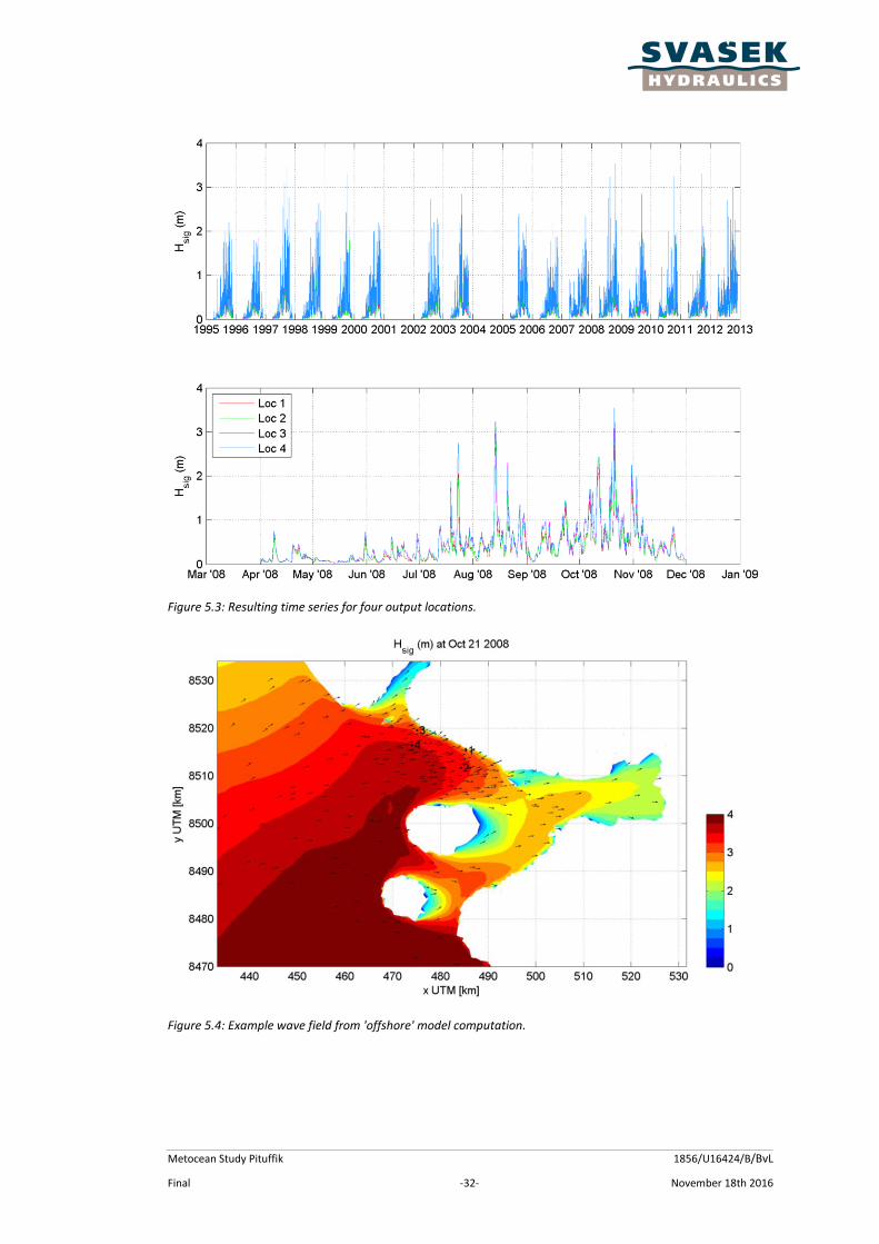
The resulting time series from the offshore model is given in Figure 5.3. Please note the missing

winter months (and 2001 and 2004, which were not present in the WWIII CSFR database). Also note

that wave action needs builds up through the year until the entire Baffin Bay is ice free and wind

fetch is at its maximum. Highest waves are usually seen in October which is consistent with the

seasonal wind analysis performed in section 3.3.

Figure 5.4 gives as an example a particularly high wave from 2008. The area of interest is sensitive

for wave from the west, and at this particular moment western winds cause high waves. Waves can

be seen refracting towards the coast line at project location. The islands in the inlet mouth have a

clear sheltering effect now angled to the west, but with waves from the south protecting the project

location.



Figure 5.3: Resulting time series for four output locations.

Figure 5.4: Example wave field from 'offshore' model computation.



5.3 Small scale 'inlet' model

Large scale CSFR winds have been shown unsuitable to model westward going waves in the inlet

itself. Instead a wind series has been constructed representative for fetch location along the intlet.

Using a small SWAN model, these winds will be translated to waves at the project location.

5.3.1 Domain, computational grid and bathymetry

A domain of the inlet has been selected in such a way that all relevant fetches for westward going

wind are incorporated. Minimum cell size is equal to the offshore model with sides of 250 m,

maximum cell sides are 500 m. The same source files are used for bathymetry. Most recent glacial

extent is taken into account on the eastward side of the model. The glaciers present in the

bathymetry source file (UCSD STRM30) extend further into the model, these areas have been

lowered to -20 m to allow wave generation.

Figure 5.5: Computational grid (upper panel) and bathymetry (lower panel) of Inlet model.



5.3.2 Spectral and directional bins

Spectral space runs from 0.05 to 2.00 Hz and is divided into 39 not equidistant bins (this means that

waves with periods of 0.5 to 20 second can be taken into account). The full circle is covered by

directional space with a total of 36 bins.

5.3.3 Ice cover

In April, May and June it is expected that parts of the inlet to the east are still covered in ice, see for

example Figure 2.5 and Figure 2.6. However shy of an extensive analysis of satellite images (outside

of the scope of this study) there is no reliable way to attain such local ice coverage patterns. Instead

ice coverage is not taken into account, which means that fetches and thus waves are overestimated

in the early months of the season. Not taking ice into consideration is thus a conservative estimate.

5.3.4 Enforced winds

In the large scale 'Offshore' model all wind conditions in the sixteen year data base have been

simulated. That was necessary due to the complex wind patterns. For the local smaller scale 'Inlet'

model, wind conditions (as determined for fetch locations in section 3.2) are much simpler. Direction

of all significant winds is from a rather narrow band from the East, and can be assumed to be

uniform over the entire model domain. As such the only variable in the wind forcing that remains is

the wind speed, which does not exceed 30 m/s between April and November. All possible conditions

can thus be covered by simulating all winds between 0 till 30 m/s with a direction of 90°N2. This

means that for each wind speed, wave conditions are known at the output locations. Winds in the

long term series can then be translated straightforwardly into long term wave data.

5.3.5 Results

Below an example is given of a wave field for winds of 14 m/s. It is clear that all locations, especially

location 1, are somewhat sheltered from the small island to the east of the project location.

Figure 5.6: Example wave field from 'inlet' model computation.

2 Please note that waves generated by wind are not very sensitive to small variations in wind direction.

Deviation by up to 20 degrees from the chosen 90 °N wind direction do not give significantly different results. This is caused by the large directional spread of wind generated waves and the fact that waves are funneled in the elongated model domain.



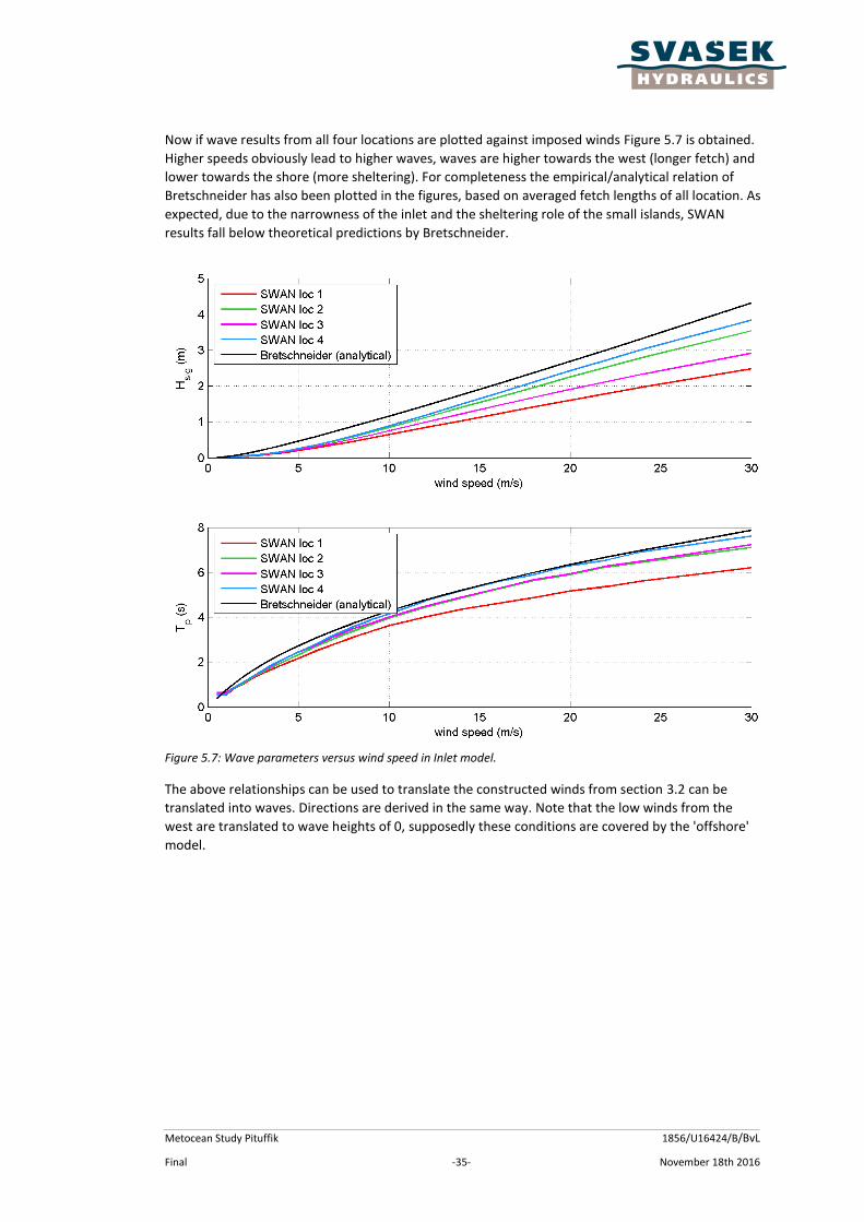
Now if wave results from all four locations are plotted against imposed winds Figure 5.7 is obtained.

Higher speeds obviously lead to higher waves, waves are higher towards the west (longer fetch) and

lower towards the shore (more sheltering). For completeness the empirical/analytical relation of

Bretschneider has also been plotted in the figures, based on averaged fetch lengths of all location. As

expected, due to the narrowness of the inlet and the sheltering role of the small islands, SWAN

results fall below theoretical predictions by Bretschneider.

Figure 5.7: Wave parameters versus wind speed in Inlet model.

The above relationships can be used to translate the constructed winds from section 3.2 can be

translated into waves. Directions are derived in the same way. Note that the low winds from the

west are translated to wave heights of 0, supposedly these conditions are covered by the 'offshore'

model.



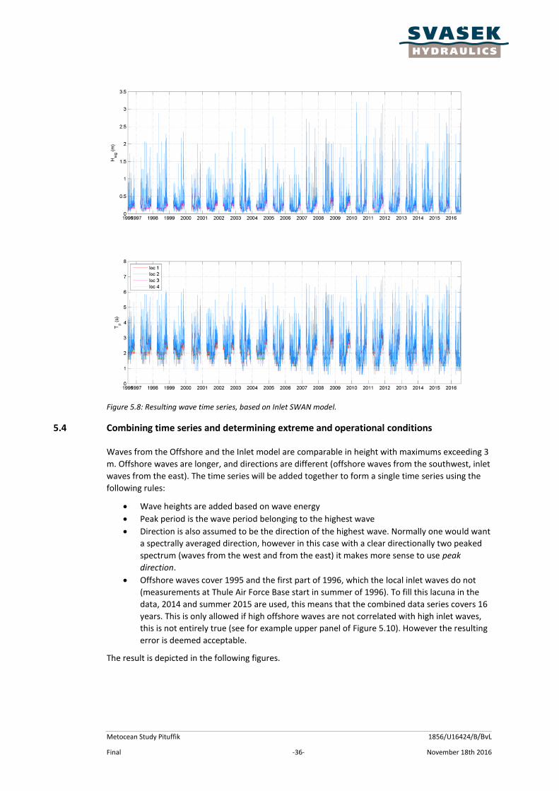
Figure 5.8: Resulting wave time series, based on Inlet SWAN model.

5.4 Combining time series and determining extreme and operational conditions

Waves from the Offshore and the Inlet model are comparable in height with maximums exceeding 3

m. Offshore waves are longer, and directions are different (offshore waves from the southwest, inlet

waves from the east). The time series will be added together to form a single time series using the

following rules:

Wave heights are added based on wave energy

Peak period is the wave period belonging to the highest wave

Direction is also assumed to be the direction of the highest wave. Normally one would want

a spectrally averaged direction, however in this case with a clear directionally two peaked

spectrum (waves from the west and from the east) it makes more sense to use peak

direction.

Offshore waves cover 1995 and the first part of 1996, which the local inlet waves do not

(measurements at Thule Air Force Base start in summer of 1996). To fill this lacuna in the

data, 2014 and summer 2015 are used, this means that the combined data series covers 16

years. This is only allowed if high offshore waves are not correlated with high inlet waves,

this is not entirely true (see for example upper panel of Figure 5.10). However the resulting

error is deemed acceptable.

The result is depicted in the following figures.



Figure 5.9: Overview of combination of offshore and inlet waves into a combined series.

Figure 5.10: Detail of 2008 of combination of offshore and inlet waves into a combined series.



5.5 Operational and extreme wave conditions

In this section the operational and extreme wave conditions are presented for the different output

locations.

The operational wave conditions are, again, presented by means of seasonal plots, see Figure 5.11,

and wave roses, see Figure 5.12. The seasonal plot, which is more or less identical for all output

locations, indicates that during the period (July till November) the highest waves are expected, but

that the direction from which these highest waves are coming varies. The wave roses in Figure 5.12

give a similar picture, in addition the wave roses also show that the direction from which the

extreme wave heights are coming also varies.

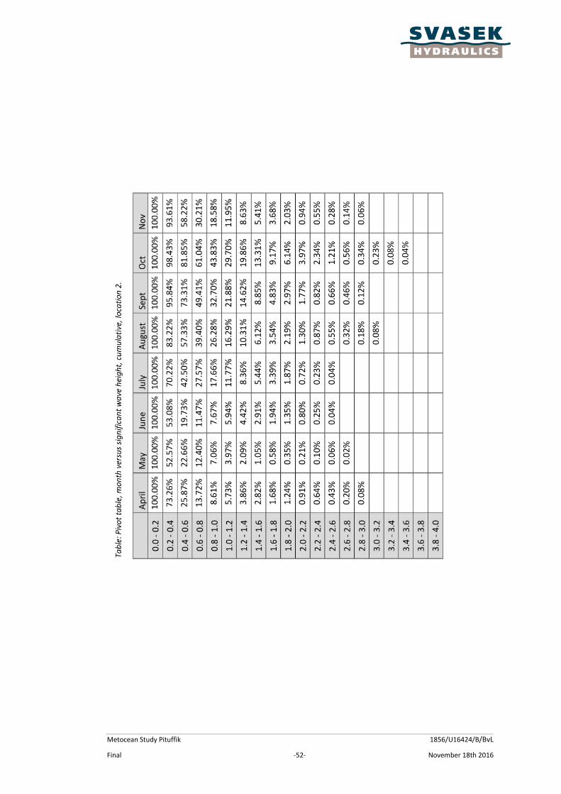
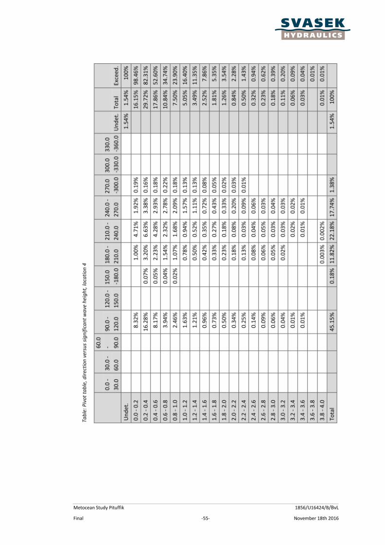
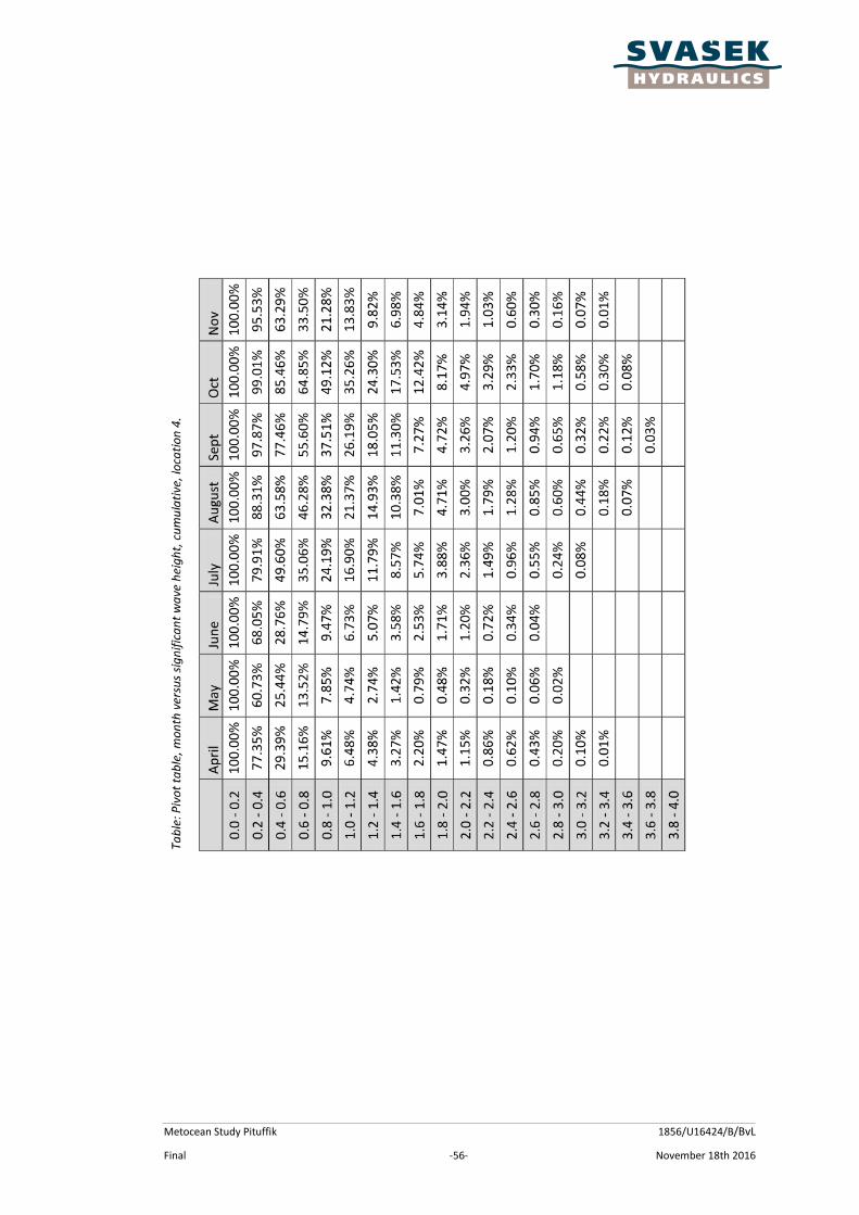
Two types of pivot tables for each location haven been included in Appendix B:

Direction versus significant wave height

Mont versus significant wave height (cumulative).

Figure 5.11. Typical seasonal plot of the operational wave conditions for location 4.



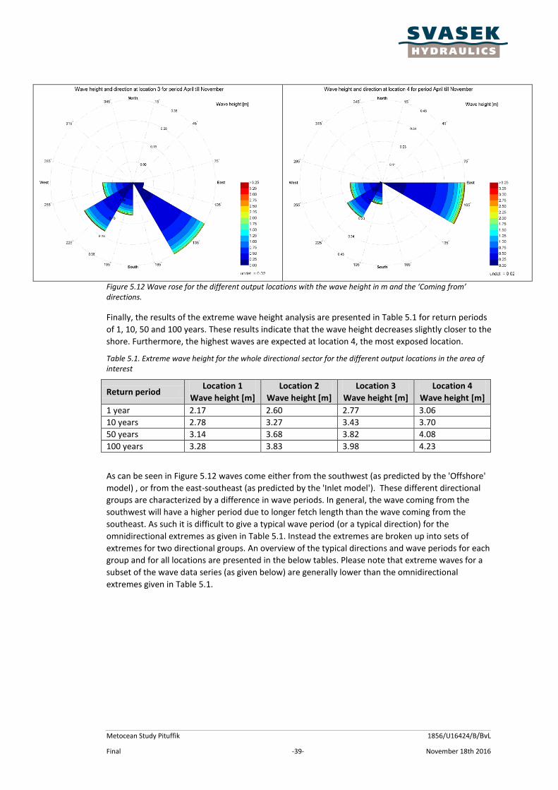
Figure 5.12 Wave rose for the different output locations with the wave height in m and the ‘Coming from’ directions.

Finally, the results of the extreme wave height analysis are presented in Table 5.1 for return periods

of 1, 10, 50 and 100 years. These results indicate that the wave height decreases slightly closer to the

shore. Furthermore, the highest waves are expected at location 4, the most exposed location.

Table 5.1. Extreme wave height for the whole directional sector for the different output locations in the area of interest


Wave height [m]

Location 2

Wave height [m]

Location 3

Wave height [m]

Location 4

Wave height [m]

1 year 2.17 2.60 2.77 3.06

10 years 2.78 3.27 3.43 3.70

50 years 3.14 3.68 3.82 4.08

100 years 3.28 3.83 3.98 4.23

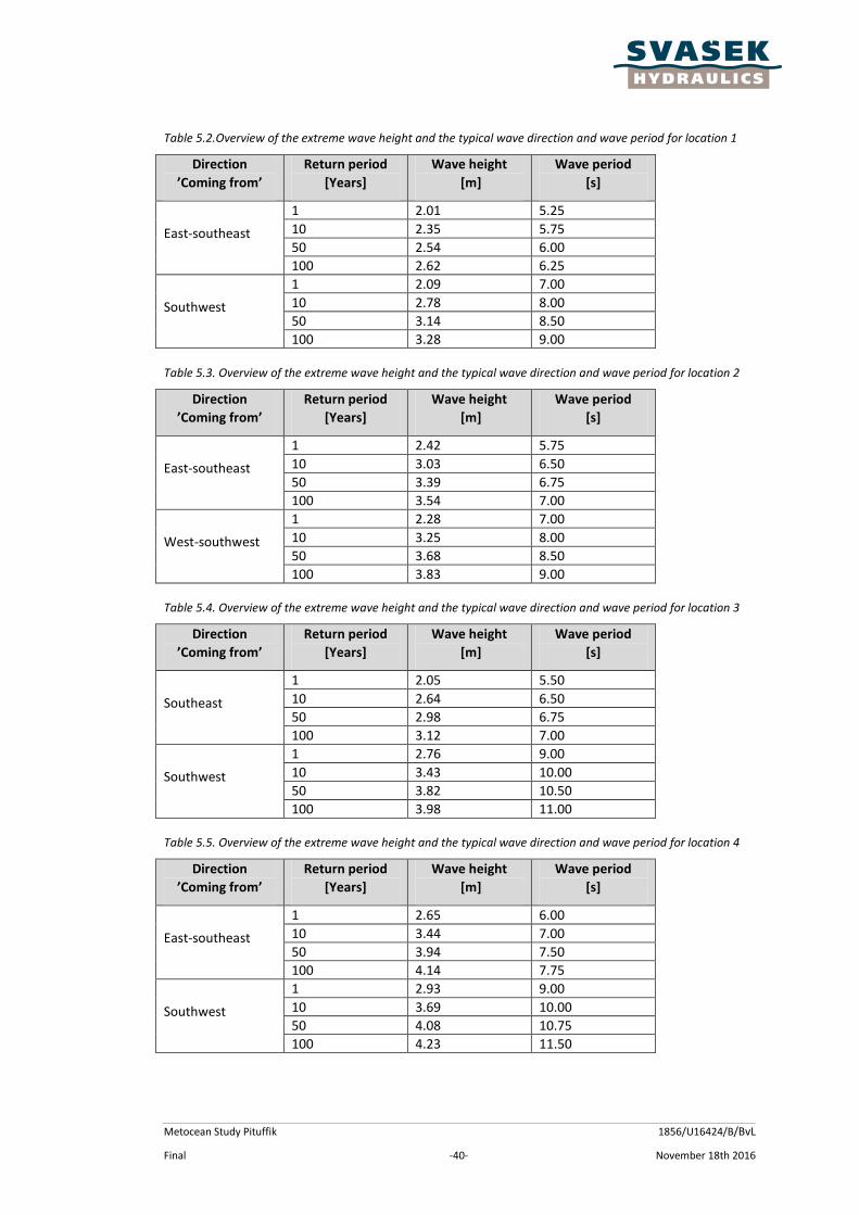
As can be seen in Figure 5.12 waves come either from the southwest (as predicted by the 'Offshore'

model) , or from the east-southeast (as predicted by the 'Inlet model'). These different directional

groups are characterized by a difference in wave periods. In general, the wave coming from the

southwest will have a higher period due to longer fetch length than the wave coming from the

southeast. As such it is difficult to give a typical wave period (or a typical direction) for the

omnidirectional extremes as given in Table 5.1. Instead the extremes are broken up into sets of

extremes for two directional groups. An overview of the typical directions and wave periods for each

group and for all locations are presented in the below tables. Please note that extreme waves for a

subset of the wave data series (as given below) are generally lower than the omnidirectional

extremes given in Table 5.1.



Table 5.2.Overview of the extreme wave height and the typical wave direction and wave period for location 1

Direction

’Coming from’

Return period

[Years]

Wave height

[m]

Wave period

[s]

East-southeast

1 2.01 5.25

10 2.35 5.75

50 2.54 6.00

100 2.62 6.25

Southwest

1 2.09 7.00

10 2.78 8.00

50 3.14 8.50

100 3.28 9.00 Table 5.3. Overview of the extreme wave height and the typical wave direction and wave period for location 2

Direction

’Coming from’

Return period

[Years]

Wave height

[m]

Wave period

[s]

East-southeast

1 2.42 5.75

10 3.03 6.50

50 3.39 6.75

100 3.54 7.00

West-southwest

1 2.28 7.00

10 3.25 8.00

50 3.68 8.50


Direction

’Coming from’

Return period

[Years]

Wave height

[m]

Wave period

[s]

Southeast

1 2.05 5.50

10 2.64 6.50

50 2.98 6.75

100 3.12 7.00

Southwest

1 2.76 9.00

10 3.43 10.00

50 3.82 10.50


Direction

’Coming from’

Return period

[Years]

Wave height

[m]

Wave period

[s]

East-southeast

1 2.65 6.00

10 3.44 7.00

50 3.94 7.50

100 4.14 7.75

Southwest

1 2.93 9.00

10 3.69 10.00

50 4.08 10.75

100 4.23 11.50



6 SUMMARY

An ice analysis has determined that the open water season (in which the project site is accessible

from the Atlantic Ocean is from late June to late October. The project site itself can be ice free as

early as April or May, however drifting ice may hinder activities well into June, July.

Twenty years of winds at the area of interest have been derived from a combination of

measurements and a high resolution model from the Canadian Meteorological Centre (HRDPS

Lancaster model). The resulting extremes are repeated in below table.

Please note that there is considerable uncertainty in the extreme winds and thus in the extreme

wave predictions, please use the results with caution.

Table 6.1. Extreme wind speeds for the project location.

Return period Extreme wind speed [m/s] Direction (Coming from)

1 year 25.0 South-East

10 years 32.2 South-East



As FINEL2D flow model of the Nares Strait has been set up and forced by satellite derived tidal

components and winds and pressures from the CSFR hind cast dataset. Sixteen years of data have

been simulated, the derived extremes are given in below table.

Table 6.2. Extreme water levels for the area of interest

Return period Maximum water level [m+msl]

1 year 1.89

10 years 2.03

50 years 2.13

100 years 2.17

Table 6.3. Extreme current velocities for the different output locations in the area of interest


Velocity [m/s]

Location 2

Velocity [m/s]

Location 3

Velocity [m/s]

Location 4

Velocity [m/s]

1 year 0.47 0.27 0.80 0.41

10 years 0.61 0.34 0.93 0.49

50 years 0.70 0.42 1.01 0.53

100 years 0.73 0.47 1.05 0.55

Mean direction

(‘Going to’) WNW WNW and ESE WNW-NW WNW-NW

Waves have been simulated by two separate SWAN models, one for offshore waves and one for local

waves generated from within the inlet. The models were forced based on a combination of CSFR

hind cast data, HRDPS Lancaster model data and measurements. The resulting extremes are

repeated in below table.

Table 6.4 Extreme wave height for the different output locations in the area of interest


Wave height [m]

Location 2

Wave height [m]

Location 3

Wave height [m]

Location 4

Wave height [m]

1 year 2.17 2.60 2.77 3.06

10 years 2.78 3.27 3.43 3.70

50 years 3.14 3.68 3.82 4.08

100 years 3.28 3.83 3.98 4.23



7 RECOMMENDATIONS

The following recommendations can be made:

If the predicted operational and extreme conditions prove critical, the accuracy of this

study could be greatly improved by conducting wind, wave and possibly current

measurements at the project site. These measurements would best be taken at the end of

summer or autumn, as ice cover is then at a minimum and conditions are most outspoken.

An extensive review of freely accessible satellite photographs fell outside of the scope of

the present study (only a cursory review was included). Such a study could help in

establishing the likelihood of drifting ice after the project location becomes ice free. A

statistical set of ice cover in the back of the estuary would also improve the performance of

the 'inlet' SWAN model, and thus the accuracy of determined wave conditions.



REFERENCES

WMO (2014). Ice Chart Colour Code Standard. Refererence: JCOMM-TR-024, WMO/TD-NO.1215,

SPA_ETSI_general_SIM04.

DNV (2005). Rules for Ships - Part 5 Ch.1 - Ships for navigation in ice. January, 2005.

Becker, J. J., D. T. Sandwell, W. H. F. Smith, J. Braud, B. Binder, J. Depner, D. Fabre, J. Factor, S. Ingalls, S-H. Kim, R. Ladner, K. Marks, S. Nelson, A. Pharaoh, R. Trimmer, J. Von Rosenberg, G. Wallace, P. Weatherall. (2009). Global Bathymetry and Elevation Data at 30 Arc Seconds Resolution: SRTM30_PLUS, Marine Geodesy, 32:4, 355-371, 2009. Saha, S., Shrinivas Moorthi, Hua-Lu Pan, Xingren Wu, Jiande Wang, Sudhir Nadiga, Patrick Tripp, Robert Kistler, John Woollen, David Behringer, Haixia Liu, Diane Stokes, Robert Grumbine, George Gayno, Jun Wang, Yu-Tai Hou, Hui-Ya Chuang, Hann-Ming H. Juang, Joe Sela, Mark Iredell, Russ Treadon, Daryl Kleist, Paul Van Delst, Dennis Keyser, John Derber, Michael Ek, Jesse Meng, Helin Wei, Rongqian Yang, Stephen Lord, Huug Van Den Dool, Arun Kumar, Wanqiu Wang, Craig Long, Muthuvel Chelliah, Yan Xue, Boyin Huang, Jae-Kyung Schemm, Wesley Ebisuzaki, Roger Lin, Pingping Xie, Mingyue Chen, Shuntai Zhou, Wayne Higgins, Cheng-Zhi Zou, Quanhua Liu, Yong Chen, Yong Han, Lidia Cucurull, Richard W. Reynolds, Glenn Rutledge and Mitch Goldberg (2010). The NCEP Climate Forecast System Reanalysis. Bull. Amer. Meteor. Soc., 91, 1015–1057. Mineral Resources Administration for Greenland (1998) . Physical Environment of Eastern Davis Strait and Northeastern Labrador Sea. Report, Copenhagen. Egbert, Gary D. and Svetlana Y. Erofeeva (2002): Efficient Inverse Modeling of Barotropic Ocean Tides. J. Atmos. Oceanic Technol., 19, 183–204.



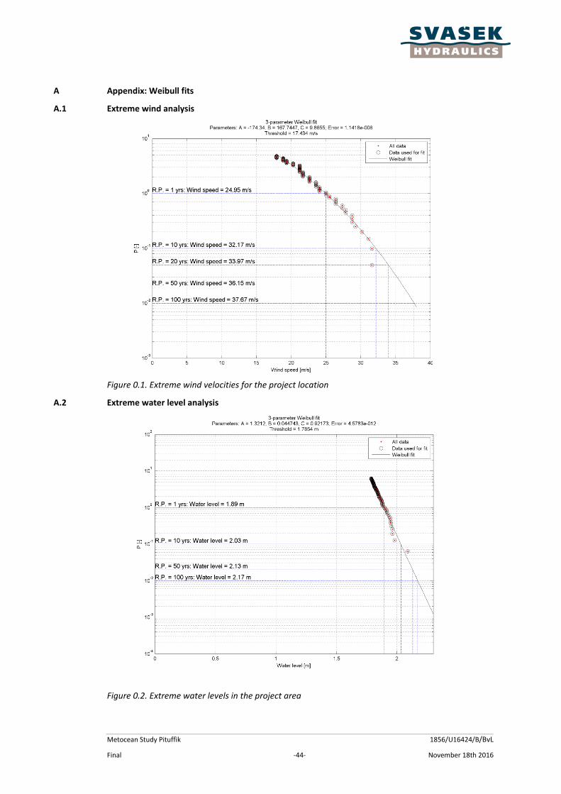
A Appendix: Weibull fits

A.1 Extreme wind analysis

Figure 0.1. Extreme wind velocities for the project location

A.2 Extreme water level analysis

Figure 0.2. Extreme water levels in the project area



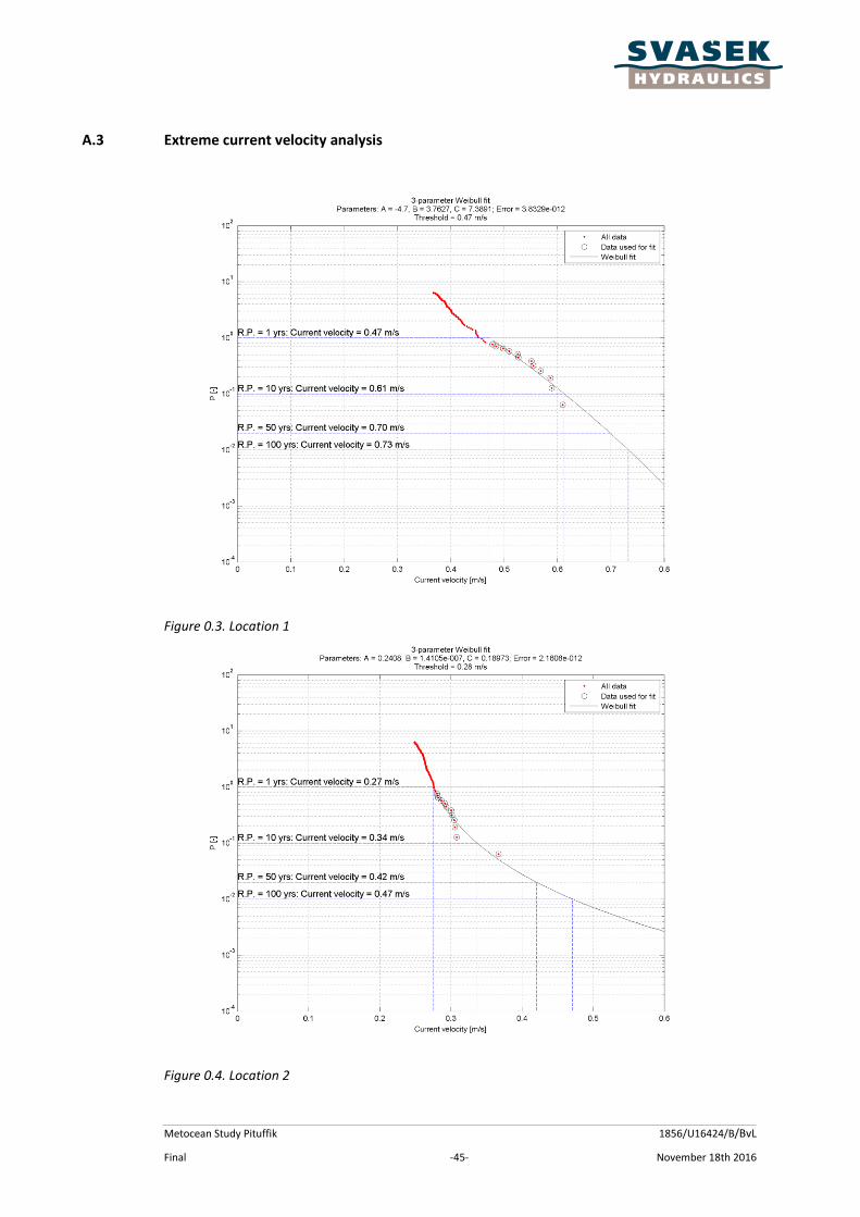
A.3 Extreme current velocity analysis

Figure 0.3. Location 1








A.4 Extreme wave analysis

Figure 0.7 Location 1.








B Appendix: Pivot tables















Date post:	10-Feb-2022
Category:	Documents
Upload:	others
View:	9 times
Download:	0 times

Metocean Study Pituffik Greenland - Dundas

Documents