106
MFIX Documentation Volume 3: Verification and Validation Manual Second Edition October, 2018 Office of Fossil Energy NETL-PUB-XXXXX

MFIX Documentation Volume 3:
Verification and Validation Manual
Second Edition
October, 2018
Office of Fossil Energy
NETL-PUB-XXXXX

Disclaimer
This report was prepared as an account of work sponsored by an agency of the United
States Government. Neither the United States Government nor any agency thereof, nor
any of their employees, makes any warranty, express or implied, or assumes any legal
liability or responsibility for the accuracy, completeness, or usefulness of any
information, apparatus, product, or process disclosed, or represents that its use would not
infringe privately owned rights. Reference therein to any specific commercial product,
process, or service by trade name, trademark, manufacturer, or otherwise does not
necessarily constitute or imply its endorsement, recommendation, or favoring by the
United States Government or any agency thereof. The views and opinions of authors
expressed therein do not necessarily state or reflect those of the United States
Government or any agency thereof.
Suggested Citation: J. Musser, A. Vaidheeswaran, and M.A. Clarke, eds. MFIX Documentation
Volume 3: Verification and Validation Manual; 2nd ed. NETL-PUB-XXXXX; NETL Technical
Report Series; U.S. Department of Energy, National Energy Technology Laboratory:
Morgantown, WV, 2018.
Keywords:
MFIX; Verification; Validation; Multiphase; Method of Manufactured Solutions; Computational
Fluid Dynamics; Discrete Element Method; Two-Fluid Model

MFIX Documentation Volume 3: Verification and Validation Manual
J. Musser1, A. Vaidheeswaran1,2, and M.A. Clarke1,2
1 Research and Innovation Center, National Energy Technology Laboratory
2 West Virginia University Research Corporation
NETL-PUB-XXXXX
October, 2018
NETL-PUB-XXXXX
NETL Contacts:
J. Musser, Principal Investigator
William A. Rogers, Technical Portfolio Lead
Bryan Morreale, Executive Director, Research and Innovation Center

MFIX Documentation Volume 3: Verification and Validation Manual
iv
This page is intentionally blank.

MFIX Documentation Volume 3: Verification and Validation Manual
v
Table of Contents
Executive Summary: ...................................................................................................... xiii
Chapter 1 : Introduction ................................................................................................. 1 1.1 Verification and Validation ...................................................................................... 1 1.2 Verification Test Selection Criteria .......................................................................... 2 1.3 Testing Frequency ..................................................................................................... 2
1.4 Case files and datasets .............................................................................................. 2 1.5 Organization .............................................................................................................. 3
Chapter 2 : Method of Manufactured Solutions (MMS) ............................................. 4 2.1 MMS Procedure Overview ....................................................................................... 4 2.2 MMS-EX01: One dimensional steady state Burger’s equation .............................. 10
2.3 MMS-EX02: One dimensional steady state heat equation ..................................... 13
2.4 MMS-EX03: One dimensional transient heat equation .......................................... 16 2.5 MMS01: Single-phase, 2D, sinusoidal functions ................................................... 24
2.6 MMS02: Two-phase, 3D, curl-based functions with constant volume fraction ..... 27 2.7 MMS03: Two-phase, 3D, curl-based functions with variable volume fraction ..... 30 2.8 MMS04: No-slip wall BC, single-phase, 3D, curl-based functions ....................... 32
2.9 MMS05: Free-slip wall BC, single-phase, 3D, curl-based functions ..................... 34 2.10 MMS06: Pressure outflow BC, single-phase, 3D, curl-based functions .............. 36
Chapter 3 : Fluid Model Code Verification Test Cases.............................................. 39 3.1 FLD01: Steady, 2D Poiseuille flow ........................................................................ 39 3.2 FLD02: Steady, 1D heat conduction ....................................................................... 41
3.3 FLD03: Steady, lid-driven square cavity ................................................................ 43
3.4 FLD04: Gresho vortex problem .............................................................................. 46
3.5 FLD05: Steady, 2D Couette flow ........................................................................... 49 3.6 FLD06: Steady, 2D multi-component species transport ......................................... 52
3.7 FLD07: Steady, 2D fully-developed, turbulent channel flow ................................ 54 3.8 FLD08: Steady, 2D turbulent pipe flow ................................................................. 57
Chapter 4 : MFIX-DEM Code Verification Test Cases .............................................. 60 4.1 DEM01: Freely-falling particle .............................................................................. 60
4.2 DEM02: Bouncing particle ..................................................................................... 65 4.3 DEM03: Two stacked, compressed particles .......................................................... 67 4.4 DEM04: Slipping on a rough surface ..................................................................... 69 4.5 DEM05: Oblique particle collision ......................................................................... 72 4.6 DEM06: Single particle, terminal velocity ............................................................. 74
References ........................................................................................................................ 78
Appendix A : Manufactured Solution Mathematical Forms ...................................... 81
A.1 Baseline 3D Manufactured Solutions .................................................................... 81 A.2 Two-Phase, 3D, Manufactured Solutions .............................................................. 82 A.3 MMS02 manufactured solutions ............................................................................ 83 A.4 MMS03 manufactured solutions ............................................................................ 86 A.5 MMS04 manufactured solutions ............................................................................ 88

MFIX Documentation Volume 3: Verification and Validation Manual
vi
A.6 MMS05 manufactured solutions ............................................................................ 90

MFIX Documentation Volume 3: Verification and Validation Manual
vii
List of Figures
Figure 1-1: Verification and validation process [3, 4]. ................................................................... 1
Figure 1-2: Scope of MFIX verification and validation activity covered in this manual. (Greyed
parts indicate future or ongoing activities not presented in the current version of this document.) 3
Figure 2-1: Procedure for order of accuracy testing. ...................................................................... 9
Figure 2-2: Observed Order, MMS Solution to 1-D steady state Burger’s equation in MFIX, using
𝑼𝒙 = 𝟏 + 𝐬𝐢𝐧(𝒙) on 𝟎 ≤ 𝒙 ≤ 𝟏. ................................................................................................. 13
Figure 2-3: Observed Order, MMS Solution to 1-D steady state heat equation in MFIX, using
𝑼𝒙 = 𝟓𝟎𝟏 + 𝒙𝟑 on 𝟎 ≤ 𝒙 ≤ 𝟓. .................................................................................................. 16
Figure 2-4: Pressure contours and velocity streamlines for 2D, single-phase, simple sinusoidal
manufactured solution on a 64x64 cell grid. ................................................................................. 25
Figure 2-5: Observed orders of accuracy for 2D, single-phase, sinusoidal manufactured solution.
(a) Superbee scheme, (b) Central scheme. .................................................................................... 26
Figure 2-6: Errors in pressure for 2D, single-phase, sinusoidal manufactured solution for grid
resolution (64x64). (a) Superbee scheme, (b) Central scheme ..................................................... 26
Figure 2-7: Gas phase momentum equation manufactured solutions for 3D, steady-state, two-phase
flow verification test case. ............................................................................................................ 27
Figure 2-8: Solids phase momentum equation manufactured solutions for 3D, steady-state, two-
phase flow verification test case. .................................................................................................. 28
Figure 2-9: Scalar field manufactured solutions for 3D, steady-state, two-phase flow verification
test case. ........................................................................................................................................ 28
Figure 2-10: Observed orders of accuracy for 3D, two-phase flows (constant volume fraction)
using (a) 𝑳𝟐 norms, and (b) 𝑳∞ norms of the discretization error. .............................................. 30
Figure 2-11: Manufactured solutions for 3D, variable volume fraction, two-phase verification. 30
Figure 2-12: Observed orders of accuracy for 3D, two-phase flows (variable volume fraction)
using (a) 𝑳𝟐 norms, and (b) 𝑳∞ norms of the discretization error. .............................................. 32
Figure 2-13: Observed orders of accuracy for no-slip wall verification (3D, single-phase flows)
using 𝑳𝟐 and 𝑳∞ norms of the discretization error. ..................................................................... 34
Figure 2-14: Observed orders of accuracy for free-slip wall verification (3D, single-phase flows)
using 𝑳𝟐 and 𝑳∞ norms of the discretization error. ..................................................................... 36

MFIX Documentation Volume 3: Verification and Validation Manual
viii
Figure 2-15: Observed orders of accuracy for pressure outflow verification using 𝑳𝟐 and 𝑳∞ norms
of the discretization error. ............................................................................................................. 38
Figure 3-1: Plane Poiseuille flow between two flat plates of length L, separated by a distance H.
....................................................................................................................................................... 39
Figure 3-2: Steady, 2D channel flow x-velocity profile (left), absolute error in x-velocity solution
(center), and observed order of accuracy (right) using four grid levels (JMAX = 8, 16, 32, 64). 41
Figure 3-3: Steady, 2D channel flow pressure profile (left) and absolute error in pressure solution
(right) using four grid levels (IMAX = 8, 16, 32, 64). .................................................................. 41
Figure 3-4: Plane-shaped slab with constant material properties and no internal heat generation is
shown with constant temperatures specified on opposing faces. The slab is assumed to be perfectly
insulated along all other faces. ...................................................................................................... 42
Figure 3-5: Steady, 1D heat-conduction. (Left) numerical solution vs analytical solution, and
(right) absolute error between the analytical and numerical solutions. ........................................ 43
Figure 3-6: Schematic of the lid-driven square cavity. ................................................................. 44
Figure 3-7: Comparison of velocities at the vertical (x=0.5) and horizontal centerlines (y=0.5) of
the cavity with Ghia et al. [16] for Reynolds number of 100 (128x128 grid). ............................. 45
Figure 3-8: Comparison of velocities at the vertical (x=0.5) and horizontal centerlines (y=0.5) of
the cavity with Ghia et al. [16] for Reynolds number of 400 (128x128 grid). ............................. 45
Figure 3-9: Comparison of velocities at the vertical (x=0.5) and horizontal centerlines (y=0.5) of
the cavity with Ghia et al. [16] for Reynolds number of 1000 (128x128 grid). ........................... 46
Figure 3-10: Comparison of velocities at the vertical (x=0.5) and horizontal centerlines (y=0.5) of
the cavity with Ghia et al. [16] for Reynolds number of 3200 (128x128 grid). ........................... 46
Figure 3-11: Exact solution for the Gresho vortex problem (shown for 𝒙, 𝒚 ∈ 𝟎. 𝟓, 𝟏 × 𝟎. 𝟓, 𝟏) 47
Figure 3-12: Comparison of vorticity by different numerical schemes with the exact solution (at
𝑻 = 𝟑𝒔). ....................................................................................................................................... 48
Figure 3-13: Couette flow between two flat plates of length L, separated by a distance H with the
upper wall moving at velocity U. .................................................................................................. 50
Figure 3-14: Couette flow with a zero pressure gradient with four grid resolutions. ................... 51
Figure 3-15: Adverse pressure gradient (-1, -2, -3 Pa) Couette flow with four grid resolutions.
Absolute error and observed order of accuracy only shown for -3 Pa pressure gradient. ............ 52
Figure 3-16: Favorable pressure gradient (1, 2, 3 Pa) Couette flow with four grid resolutions.
Absolute error and observed order of accuracy only shown for 3 Pa pressure gradient. ............. 52

MFIX Documentation Volume 3: Verification and Validation Manual
ix
Figure 3-17: Multicomponent species transport. .......................................................................... 53
Figure 3-18: Turbulent flow in a 2D channel ............................................................................... 55
Figure 3-19: 2D, fully developed, turbulent channel flow with the DNS data of Lee and Moser
[19]; (Left) Velocity profile; (Right) Non-dimensionalized channel width and velocity profile. 57
Figure 3-20: Turbulent flow in a pipe ........................................................................................... 57
Figure 3-21: 2D, turbulent pipe flow with the experimental data of DNS data of Zagarola and Smits
[20]; (Left) Velocity profiles; (Right) Nondimensionalized channel width and velocity profile. 59
Figure 4-1: A particle with radius 𝒓𝒑 falling onto a fixed wall from an initial height of 𝒉𝟎 where
𝒈 is the gravitational force, 𝑭𝑪 is repulsive particle-wall collision force, 𝒗𝒄 is the pre-collision
particle velocity, and 𝒗𝒓 is the post-collision particle velocity. ................................................... 61
Figure 4-2: Comparison of analytical solution and DEM results for a freely-falling particle using
the Euler time-stepping method for varying restitution coefficient, normal spring coefficient, 𝒌𝒏 =𝟏𝟎𝟒 N•m-1. (Left) Particle center position; analytical solutions shown as continuous lines, MFIX-
DEM results as points. (Right) Percent absolute relative error between the analytical and MFIX-
DEM particle center positions. ..................................................................................................... 63
Figure 4-3: Comparison of analytical solution and DEM results for a freely-falling particle using
the Euler time-stepping method for varying restitution coefficients, and normal spring coefficient,
𝒌𝒏 = 𝟏𝟎𝟓 N•m-1. (Left) Particle velocities; analytical solutions shown as continuous lines, MFIX-
DEM results as points. (Right) Percent absolute relative error between the analytical and MFIX-
DEM particle velocities. ............................................................................................................... 64
Figure 4-4: Difference between analytical solution and MFIX-DEM results for a freely-falling
particle with varying restitution coefficient and normal spring coefficient, 𝒌𝒏 = 𝟏𝟎𝟓 N•m-1. Euler
method shown as solid line. Adams-Bashforth method shown as dashed lines. (Left) Difference in
particle position. (Right) Difference in particle velocity. ............................................................. 65
Figure 4-5: Comparison between the analytic solution from a hard-sphere model (solid lines) and
MFIX-DEM (symbols) of the maximum height reached after the kth wall collision for a freely
falling particle. Three values for the normal spring coefficient are used (left to right) with six
restitution coefficients. .................................................................................................................. 66
Figure 4-6: Percent relative difference between the analytic solution for a hard-sphere model and
MFIX-DEM of the maximum height reached after the kth wall collision for a freely falling particle.
Three values for the normal spring coefficient are used (left to right) with six restitution
coefficients. ................................................................................................................................... 67
Figure 4-7: Two smooth spherical particles stacked between two fixed walls so that the system is
always under compression. A sketch of the problem mechanics is provided along with force
balances for the lower and upper particles. ................................................................................... 67

MFIX Documentation Volume 3: Verification and Validation Manual
x
Figure 4-8: Comparison between the fourth-order Runge-Kutta solution (solid line) and MFIX-
DEM simulation (open symbols) for the center position of two stacked particles compressed
between fixed walls for a restitution coefficient of 1. The absolute percent relative errors are shown
as dashed lines............................................................................................................................... 69
Figure 4-9: A spherical particle with finite translational velocity and zero angular velocity is placed
on a rough surface. Forces acting on the particle are indicated. ................................................... 70
Figure 4-10: Comparison between the analytical solution (solid line) and MFIX-DEM simulation
(open symbols) of a particle with radius 𝒓𝒑 slipping on a rough surface for various friction
coefficients. (left) Dimensionless slip time end and (right) dimensionless equilibrium tangential,
𝒖, and angular, 𝝎, velocities. ........................................................................................................ 71
Figure 4-11: (a) Experimental setup of Kharaz, Gorham, and Salman [26] of a particle striking a
fixed, angled anvil. (b) Simulation setup whereby the particle is given an initial velocity to replicate
the particle striking an angled surface. ......................................................................................... 72
Figure 4-12: Particle-wall oblique collision results for the linear spring-dashpot model (solid line),
Hertzian model (dashed line), and experimental data (symbols) of Kharaz, Gorham, and Salman
[26]. ............................................................................................................................................... 74
Figure 4-13: Particle-particle oblique collision results for the linear spring-dashpot model (solid
line), Hertzian model (dashed line), and experimental data (symbols) of Kharaz, Gorham, and
Salman [26]. .................................................................................................................................. 74
Figure 4-14: A single spherical particle initially at rest is released in a uniform, vertical air flow.
The dominant forces acting on the particle are the gas-solids drag force, 𝑭𝒅, and the gravitational
force, 𝒈. ......................................................................................................................................... 75
Figure 4-15: Comparison of the particle velocity evolution obtained by equation (4-17) and MFIX-
DEM. ............................................................................................................................................. 77
Figure 4-16: Absolute percent relative difference between particle velocity evolution obtained by
equation (4-17) and MFIX-DEM. (left) Simulations with one-way gas-solids coupling. (right)
Fully coupled simulations. ............................................................................................................ 77

MFIX Documentation Volume 3: Verification and Validation Manual
xi
List of Tables
Table 2-1: Summary of MMS tests by feature................................................................................ 4
Table 2-2: Observed Order, p, for steady state Burger’s equation using 𝑼𝒙 = 𝟏 + 𝐬𝐢𝐧(𝒙) on 𝟎 ≤𝒙 ≤ 𝟏. ............................................................................................................................................ 12
Table 2-3: Observed Order, p, for steady state heat equation using 𝑼𝒙 = 𝟓𝟎𝟏 + 𝒙𝟑 on 𝟎 ≤ 𝒙 ≤𝟓. ................................................................................................................................................... 16
Table 2-4: Parameters used in MMS applied to transient heat conduction .................................. 18
Table 2-5: Mixed analysis refinement factors [10]; highlighted row for expected spatial order =2,
and expected temporal order = 1 based on known MFIX routines ............................................... 20
Table 2-6: L norms and the observed order for the unsteady heat equation – temporal order of
accuracy ........................................................................................................................................ 21
Table 2-7: L norms and the observed order for the unsteady heat equation – spatial order of
accuracy ........................................................................................................................................ 22
Table 2-8: L norms and the observed order in combined order analysis for the unsteady heat
equation – temporal order of accuracy.......................................................................................... 24
Table 2-9: L norms and the observed order in combined order analysis for the unsteady heat
equation – spatial order of accuracy ............................................................................................. 24
Table 3-1: Summary of MFIX-FLD tests by feature .................................................................... 39
Table 3-2: Total kinetic energy of the flow field compared to the exact (initial) value for various
spatial discretization schemes. ...................................................................................................... 49
Table 3-3: Average L2 Norms for the gas pressure (Pg), x-axial velocity (Ug) and y-axial velocity
(Vg) for various spatial discretization schemes. .......................................................................... 49
Table 3-4: Average species mass fractions at the outflow and average L2 Norms between the
analytical and MFIX species mass fraction for the well-mixed fluid. .......................................... 54
Table 4-1: Summary of MFIX-DEM tests by feature ................................................................... 60

MFIX Documentation Volume 3: Verification and Validation Manual
xii
Acronyms and Abbreviations
BC Boundary Condition
CFD Computational Fluid Dynamics
CV Control Volume
CI Continuous Integration
DEM Discrete Element Model
EE Eulerian-Eulerian
MFIX Multiphase Flow with Interphase eXchanges
MMS Method of Manufactured Solutions
MPPIC Multiphase Particle-In-Cell
PDE Partial Differential Equation
SQA Software Quality Assurance
TFM Two-Fluid Model
V&V Verification and Validation
UQ Uncertainty Quantification

MFIX Documentation Volume 3: Verification and Validation Manual
xiii
Executive Summary:
The MFIX Verification and Validation Manual aims to document verification tests and validation
cases for the MFIX suite. Additionally, this manual attempts to capture best practices for
verification and validation as part of a broader approach to software quality assurance. The goal is
to perform a systematic verification of features available in MFIX for correctness and numerical
accuracy.
Contributors:
(Alphabetical by last name)
Sofiane Benyahia
Aniruddha Choudhary
Mary Ann Clarke
Jean-François Dietiker
William Fullmer
Janine Galvin
Aytekin Gel
Chris Guenther
Tingwen Li
Mark Meredith
Aaron Morris
Jordan Musser
Thomas O’Brien
Sreekanth Pannala
William Rogers
Mehrdad Shahnam
Madhava Syamlal
Avinash Vaidheeswaran
The editors thank all contributors, especially our colleagues in the NETL Multiphase Flow Science
Group, for their assistance and feedback in the creation and maintenance of this document.

MFIX Documentation Volume 3: Verification and Validation Manual
1
Chapter 1: Introduction
The MFIX Verification and Validation Manual, referred to herein as the V&V Manual, aims to
document verification tests and validation cases for the MFIX suite. Additionally, this manual
attempts to capture best practices for V&V as part of a broader approach to software quality
assurance (SQA). The goal is to perform a systematic verification of features available in the
code for correctness and numerical accuracy. Future work will include validation cases to assess
the suitability of the physical models implemented within MFIX. The V&V Manual also serves
as a guide for periodic and automated testing of the software by the developers.
1.1 Verification and Validation
For the purpose of this manual, the terms verification and validation are defined as follows [1]:
• Verification: The process of determining that a numerical model implementation accurately
represents the developer's conceptual description of the model and the mathematical solution
to the model.
• Validation: The process of determining the degree to which a model is an accurate
representation of the real world from the perspective of the intended uses of the model.
Roache [2] succinctly describes verification as an assessment on “solving the equations right”
whereas validation is “solving the right equations.” Figure 1-1 illustrates the relationship
between verification and validation processes schematically.
Figure 1-1: Verification and validation process [3, 4].
Verification deals with the mathematics of the simulation and involves assessing the correctness
of the computer code and numerical algorithms (i.e., code verification) as well as the accuracy of
the numerical solution (i.e., solution verification). Validation deals with the physics of the
problem and assesses whether the selected mathematical model satisfactorily predicts the physics

MFIX Documentation Volume 3: Verification and Validation Manual
2
of interest. Roache [5] further noted the distinction between verification and validation as,
“Verification is a mathematics issue; not a physics issue.” Hence, verification precedes
validation.
1.2 Verification Test Selection Criteria
Verification test cases are selected based upon the following criteria:
• Each test case should exercise one or more sub-models for a physical phenomenon
• Simulations must be computationally inexpensive to facilitate regular testing
• There should be minimal overlap between tests
The preference and thereby quality of a test is assessed on the following criteria:
• (Most preferable) Examination of numerical error between the exact solution and the
numerical solution for problems where an analytical solution is available (i.e.,
verification using method of exact solutions) or a manufactured solution is obtainable
• (Less preferable) Comparison of numerical solutions to established results in literature
(i.e., similar to validation, but using benchmark problems)
• (Least preferable) Comparison of numerical solutions to results obtained from previous
versions of the same code (i.e., regression test) or from another verified code (i.e., code
comparison)
1.3 Testing Frequency
Cases presented within this document are tested at various intervals as part of the SQA process.
Before 2014, code integrity in MFIX was tracked through a series of nightly regression tests
based on an open source software testing framework called QMTest, which provided a single
snapshot on a daily basis [6]. This method was replaced by a continuous integration (CI) server
for greater testing and archival flexibility.
Cases that execute quickly are tested whenever modifications are committed to the source code
repository to quickly detect any issues generated by the changes. However, computationally
burdensome verification and validation cases are tested less frequently to prevent overwhelming
the CI server. A summary table at the start of each chapter indicates the frequency at which each
case is tested.
1.4 Case files and datasets
Case files and datasets for the tests outlined in this document are provided with the MFIX source
code under the mfix/tests directory. All presented data are representative of results from the
current MFIX release unless explicitly noted.

MFIX Documentation Volume 3: Verification and Validation Manual
3
1.5 Organization
Chapter 2 provides verification tests that use the Method of Manufactured Solution (MMS) to
determine whether the observed order of error reduction with grid refinement matches the formal
order. Order testing with MMS is considered to be a very rigorous procedure for code
verification.
Chapters 3 and 4 provide verification tests that use benchmark solutions of simple problems to
test the two main models of the MFIX software suite: (1) Two-Fluid Model, and (2) Discrete
Element Model. This process examines various aspects of the code but only for problems with
significantly simplified physics.
Figure 1-2 shows the scope of the V&V activity covered in this manual.
Figure 1-2: Scope of MFIX verification and validation activity covered in this manual. (Greyed parts indicate
future or ongoing activities not presented in the current version of this document.)

MFIX Documentation Volume 3: Verification and Validation Manual
4
Chapter 2: Method of Manufactured Solutions (MMS)
Order of accuracy testing (or ‘order testing’) is considered a rigorous method for performing
code verification. During order testing, the formal order of accuracy of a numerical scheme is
compared to the observed order of accuracy. The observed order is the order at which the
discretization error (which is the difference between the numerical solution to the discrete
equations and the exact solution to the PDEs) decreases with systematic mesh refinement.
However, the exact solution to a PDE is unknown for most practical problems. In this scenario,
the Method of Manufactured Solutions (MMS) [7] can be used where a selected analytical
function (called a ‘manufactured solution’) is forced to be the exact solution by modifying the
PDE through additional source terms.
The MMS test cases presented in this chapter are summarized in Table 2-1. These test cases offer
an increasing level of computational complexity to isolate any potential problems in the source
code. Three explanatory test cases that employ various simplifying assumptions are provided to
assist the reader in understanding the MMS. Additional test cases were selected based upon their
ability to invoke various parts of the MFIX code, and present physically acceptable data. All
cases are executed in serial mode unless explicitly noted.
Table 2-1: Summary of MMS tests by feature
Fre
qu
ency
†
Dim
ensi
on
Mu
ltip
ha
se
Co
nti
nu
ity
Mo
men
tum
Th
erm
al
En
erg
y
Sp
ecie
s M
ass
Gra
nu
lar
En
erg
y
Tu
rbu
len
ce
No
-sli
p W
all
BC
Fre
e-s
lip
Wa
ll B
C
Pre
ssu
re O
utf
low
Dis
trib
ute
d M
emo
ry
Sh
are
d M
em
ory
MMS-EX01 X 1D ✓
MMS-EX02 X 1D ✓
MMS-EX03 X 1D ✓
MMS01 M 2D ✓ ✓
MMS02 M 3D ✓ ✓ ✓ ✓
MMS03 M 3D ✓ ✓ ✓
MMS04 M 3D ✓
MMS05 M 3D ✓
MMS06 M 3D ✓
† C-Incorporated into the continuous integration server;
M-Monthly; Q-Quarterly; D-Disabled; X-Manual
2.1 MMS Procedure Overview
To better instruct the reader, the procedure for using a MMS to conduct an order of accuracy test
is summarized by example [8, 9]:

MFIX Documentation Volume 3: Verification and Validation Manual
5
1. Allow any partial differential equation in n-dimensions to be represented through the
notation:
𝐿[𝑢(𝑥1, 𝑥2, ⋯ , 𝑥𝑛, 𝑡)] = 0 (2-1)
For example, a one-dimensional non-linear Burger equation:
𝑢𝑡 + 𝑢𝑢𝑥 = 𝛼𝑢𝑥𝑥 (2-2)
would be represented as:
𝐿[𝑢(𝑥, 𝑡)] = 𝑢𝑡 + 𝑢𝑢𝑥 − 𝛼𝑢𝑥𝑥 = 0 (2-3)
2. Make up a manufactured solution to the proposed partial differential equation. The
chosen solution does not need to represent the solution to a physical problem. The MMS
is a mathematical exercise to determine if a piece of software will accurately calculate a
solution to its prescribed numerical order.
For example, allow: 𝑈(𝑥, 𝑡) = 𝐴 + sin(𝑥 + 𝐶𝑡) where 𝐴 and 𝐶 are constants, to be a
solution to 𝐿[𝑢(𝑥, 𝑡)].
The key is that whatever one chooses for 𝑈(𝑥, 𝑡), it must be mathematically analytic,
meaning fully differentiable with continuous derivatives to at least the order of the partial
differential equation one is trying to solve over the full domain of the problem. In this
example, the constant value function 𝐴 and the sinusoidal function sin(𝑥 + 𝐶𝑡) obviously
meet these criteria. Do not choose functions that display discontinuities of any type for
any derivative if the domain of interest extends through those discontinuities. In
addition, it is important that all terms in a given manufactured solution are of similar
magnitude. This assures that solutions are not dominated by a single term which might
skew order of accuracy results.
It is essential to choose solutions that do not engage physical constraints within the code
that is under evaluation. For example, MFIX issues an error message and stops all
calculations if the temperature in any computational cell falls below 250 Kelvin. So, if
testing the energy equation, the manufactured solution should never present a value less
than 250, as this value is contextually interpreted as an unphysical temperature.
3. Apply the manufactured solution to the partial differential equation being solved. This
means create the derivatives represented in the original problem and substitute them into
the equation.

MFIX Documentation Volume 3: Verification and Validation Manual
6
For example, using 𝑈(𝑥, 𝑡) = 𝐴 + sin(𝑥 + 𝐶𝑡) as a manufactured solution for
𝐿[𝑢(𝑥, 𝑡)] = 𝑢𝑡 + 𝑢𝑢𝑥 − 𝛼𝑢𝑥𝑥 = 0 requires
𝐿[𝑢(𝑥, 𝑡)]𝑈(𝑥,𝑡) =𝜕
𝜕𝑡(𝑈(𝑥, 𝑡)) + 𝑈(𝑥, 𝑡)
𝜕
𝜕𝑥(𝑈(𝑥, 𝑡)) − 𝛼
𝜕2
𝜕𝑥2(𝑈(𝑥, 𝑡)) = 0
(2-4)
After substitution,
𝐿[𝑢(𝑥, 𝑡)]𝑈(𝑥,𝑡) = 𝐶 cos(𝑥 + 𝐶𝑡) + (𝐴 + sin(𝑥 + 𝐶𝑡))(cos(𝑥 + 𝐶𝑡)) − 𝛼(− sin(𝑥 + 𝐶𝑡)) = 0 (2-5)
Or,
𝐿[𝑢(𝑥, 𝑡)]𝑈(𝑥,𝑡) = (𝐴 + 𝐶) cos(𝑥 + 𝐶𝑡) + sin(𝑥 + 𝐶𝑡) cos(𝑥 + 𝐶𝑡) + 𝛼 sin(𝑥 + 𝐶𝑡) = 0 (2-6)
𝐿[𝑢(𝑥, 𝑡)]𝑈(𝑥,𝑡) represents what are called source terms in MMS. Thinking about this
using notation:
𝐿[𝑢(𝑥, 𝑡)] = 0 = 𝐿[𝑢(𝑥, 𝑡)]𝑈(𝑥,𝑡) (2-7)
Or,
𝐿[𝑢(𝑥, 𝑡)] − 𝐿[𝑢(𝑥, 𝑡)]𝑈(𝑥,𝑡) = 0 (2-8)
After calculation, any arithmetic difference between the numerical solution and the exact
solution is assumed to originate from the numerical method.
4. To properly solve a partial differential equation of the form 𝐿[𝑢(𝑥1, 𝑥2, ⋯ , 𝑥𝑛, 𝑡)] = 0,
one needs appropriately chosen initial and boundary values.
So, by example, assume that the physical domain of interest is 𝑥𝜖[0,1] and allow
𝑡𝜖[0,∞).
First, force the initial condition of 𝑢(𝑥, 0) to align with that of the manufactured solution,
𝑈(𝑥, 0) by choosing,
𝑢(𝑥, 0) = 𝑈(𝑥, 0) = 𝐴 + sin(𝑥 + 𝐶(0)) = 𝐴 + sin(𝑥) (2-9)
Then, select boundary conditions in any meaningful way, forcing alignment between the
proposed partial differential equation and the manufactured solution. For example,
perhaps fixed boundary conditions are useful. These are sometimes called Dirichlet
boundary conditions. Applying a fixed boundary condition means choose functions for
fixed boundary locations that will be maintained through all time-steps. It does not mean

MFIX Documentation Volume 3: Verification and Validation Manual
7
that a boundary must have the same value for all time, although that is a possibility (the
function chosen might be a constant).
So, for this example, an appropriate fixed boundary condition would be:
𝑢(0, 𝑡) = 𝑈(0, 𝑡) = 𝐴 + sin(0 + 𝐶𝑡) = 𝐴 + sin(𝐶𝑡)
𝑢(1, 𝑡) = 𝑈(1, 𝑡) = 𝐴 + sin(1 + 𝐶𝑡)
(2-10)
Note that in this example, the fixed (Dirichlet) boundary condition varies with time.
The type of boundary condition is insignificant to the method of manufactured solutions.
One can easily choose Neumann (flux conditions at the boundary), Cauchy (a mix of
fixed conditions and at least one derivative in the direction of the normal of the
boundary), Robin (weighted combinations of Neumann and Dirichlet conditions over all
boundaries) or mixed conditions (different boundary condition types on different subsets
of the boundary) as each partial differential equation application is explored.
By example, a different solution to our proposed problem will occur if we shift to a mixed
boundary condition such that:
𝑢(0, 𝑡) = 𝑈(0, 𝑡) = 𝐴 + sin(0 + 𝐶𝑡) = 𝐴 + sin(𝐶𝑡)(𝐷𝑖𝑟𝑖𝑐ℎ𝑙𝑒𝑡)
𝜕
𝜕𝑥(𝑢(1, 𝑡)) =
𝜕
𝜕𝑥(𝑈(1, 𝑡)) =
𝜕
𝜕𝑥(𝐴 + sin(1 + 𝐶𝑡)) = cos(1 + 𝐶𝑡)(𝑁𝑒𝑢𝑚𝑎𝑛𝑛)
(2-11)
In this way, the method of manufactured solutions allows the investigator to examine
how the application of different boundary conditions affects the overall veracity of
numerical approximations within the context of problems where solutions can be found
through explicit hand calculation.
5. Theoretically, when a manufactured exact solution is known, computer algorithms
applied to imitate that result should converge systematically toward exactness as the
calculation space is ever more refined. Ideally, one might expect an eventual numerical
result to differ from an exact solution by no more than 𝒪(machine epsilon). Of course,
the theoretical threshold of solution quality varies widely from this value as there are few
calculations that can be held to such a high standard. For example, computers estimate all
transcendental functions with truncated power series on computers, regardless of what a
programmer types into code, and these functions are inherently burdened with this
approximation error.
However, one can systematically refine a mesh and recalculate the solution to proposed
problems in search of exactness. Once the arithmetic difference between the discretized
solution and a manufactured solution remains constant, regardless of further mesh
refinement, one has discovered the best numerical solution possible for a given code and

MFIX Documentation Volume 3: Verification and Validation Manual
8
a given problem. If the error between discretized solution and manufactured solution is
acceptable by some standard, a code can be considered numerically verified. Note that
this verification is limited to those code components invoked when setting up a MMS.
As is the case for MFIX, most codes are far too complex to complete a full verification in
a single MMS.
6. Global discretization error, 𝐷𝐸ℓ , is the arithmetic difference between the computer
(approximate or discrete) evaluation of the manufactured solution to a by hand (exact)
solution. The script ℓ is to remind the user of mesh ℓevel.
Rather than evaluate discretization error one cell at a time, one can further consider
global discretization error through various mathematical norms. An 𝐿1norm is an
average absolute error over all cell locations (𝑖𝑗𝑘 = 1,… , 𝑛) in a calculation represented
through an absolute difference.
𝐿1:‖𝐷𝐸ℓ‖1 =∑ |𝐷𝐸ℓ,𝑖𝑗𝑘|
𝑛𝑖𝑗𝑘=1
𝑛 (2-12)
An 𝐿2 norm is a root mean square error over all cell locations (𝑖𝑗𝑘 = 1, … , 𝑛).
𝐿2:‖𝐷𝐸ℓ‖2 = √∑ |𝐷𝐸ℓ,𝑖𝑗𝑘|
2𝑛𝑖𝑗𝑘=1
𝑛
(2-13)
An 𝐿∞ norm is the maximum error in any single cell location (𝑖𝑗𝑘 = 1,… , 𝑛).
𝐿∞ = ‖𝐷𝐸ℓ‖∞ = max𝑖𝑗𝑘
|𝐷𝐸ℓ,𝑖𝑗𝑘| (2-14)
7. As mesh size, ℎ, changes, one collects the normed values of global discretization error
and applies them to create an observed order, 𝑝.
𝑝 =𝑙𝑛 (
‖𝐷𝐸ℓ+1‖‖𝐷𝐸ℓ‖
)
𝑙𝑛 (ℎℓ+1
ℎℓ)
=𝑙𝑛 (
‖𝐷𝐸ℓ+1‖‖𝐷𝐸ℓ‖
)
𝑙𝑛(𝑟)
(2-15)
In this notation, mesh level, ℓ, is largest at the coarsest mesh, and smallest at the most
refined mesh. One will also see the observed order formula where the ratio between two
mesh sizes (as seen in the denominator of 𝑝) is called a mesh refinement factor, 𝑟.
Furthermore, the term grid size measure, ℎ̆, is a ratio formed by comparing the number of

MFIX Documentation Volume 3: Verification and Validation Manual
9
divisions making up the finest mesh to the current mesh. Figure 2-1 works to clarify
these definitions within the context of observed order, and illustrates an observed order
plot where 𝑟 = 2, between subsequent mesh levels. Note that the use of grid size
measure eliminates the need for any units in graphical representations of observed order.
Figure 2-1: Procedure for order of accuracy testing.
Ideally, one makes as many simulations as necessary to show that limℎ→0
𝑝 is constant,
thereby inferring that the best possible numerical solution has been made, and further
simulation is unwarranted.
Note that the norm chosen for the calculation of observed order may affect the outcome
of this assessment. For example, the most challenging norm related above is 𝐿∞, as it
isolates the largest error in any given simulation. The least challenging norm is 𝐿1, as it
will most easily mask localized high level error with areas of good agreement across any
given domain.
5
1
𝑝1
Ob
serv
ed O
rder
, 𝑝
Grid Size Measure, ℎ̆
4
3
2
1
16
8
4
2
1
Mesh Level,ℓ
Grid Size
Measure,ℎ̆ Mesh size,ℎ Observed
Order, 𝑝
𝑝4
𝑝3
𝑝2
𝑝1 2 4 8
𝑝2 𝑝3
𝑝4 1.0
1.5
2.0
2.5

MFIX Documentation Volume 3: Verification and Validation Manual
10
2.2 MMS-EX01: One dimensional steady state Burger’s equation
2.2.1 Description
The gas-phase momentum equations in MFIX have the following generalized form:1
𝜕
𝜕𝑡(휀𝑔𝜌𝑔𝑢𝑔𝑖) +
𝜕
𝜕𝑥𝑗(휀𝑔𝜌𝑔𝑢𝑔𝑗𝑢𝑔𝑖) = −
𝜕𝑃𝑔
𝜕𝑥𝑖+
𝜕𝜏𝑔𝑖𝑗
𝜕𝑥𝑗+ 휀𝑔𝜌𝑔𝑔𝑖 + 𝒮𝑔𝑖
(2-16)
where,
𝜏𝑔𝑖𝑗 = 2𝜇𝑔 [1
2(𝜕𝑢𝑔𝑖
𝜕𝑥𝑗+
𝜕𝑢𝑔𝑗
𝜕𝑥𝑖) −
1
3
𝜕𝑢𝑔𝑘
𝜕𝑥𝑘𝛿𝑖𝑗]
(2-17)
To build on the previous example, the momentum equations can be recast as the one-dimensional
steady state Burger’s equation by imposing the following simplifying assumptions:2
1. A steady state simulation is needed to remove the momentum equations’ transient term.
2. Calculations are restricted to one dimension.
3. The domain is of unit length in the x-axial direction: 𝑥𝜖[0,5].
4. The gas volume fraction and density are set to one, 휀𝑔 = 1 and 𝜌𝑔 = 1.
5. The gas viscosity is chosen as 𝜇𝑔 = 3/4.
6. Gravity and all other source terms are set to zero, 𝑔 = 0 and 𝒮𝑔𝑖 = 0.
7. Finally, because the pressure solver is integrated with the momentum equations, it is
important to decouple the pressure correction step from the calculation.
The momentum equations with the above simplifications reduce to the one-dimensional Burger’s
equation,
𝑢𝑔
𝜕𝑢𝑔
𝜕𝑥−
𝜕2𝑢𝑔
𝜕𝑥2= 0
(2-18)
where the subscript indicating dimensionality has been dropped for notational clarity.
Following the method of manufactured solutions, the partial differential equation is recast as:
𝐿(𝑥) = 𝑢𝑢𝑥 − 𝑢𝑥𝑥 (2-19)
MMS requires the selection of a manufactured solution. Arbitrarily, choose any suitable analytic
form of appropriate continuous, differential order. In this case, note that whatever manufactured
1 The conservative form of the fluid momentum equations is presented here, however, the non-conservative form is
solved in MFIX. The non-conservative form is obtained by subtracting the continuity equation from the conservative
form. 2 Assumptions that reduce model complexity are typically avoided when using the MMS. However, this example
intentionally simplifies the momentum equations to make the example easier to follow.

MFIX Documentation Volume 3: Verification and Validation Manual
11
solution is chosen must be continuously differentiable through its second derivative. Aside from
asymptotic functions that may exhibit unphysical local changes, most any analytic function will
be a suitable choice for this application. So, keeping things simple, as in the prior explanation,
𝑈(𝑥) = 0.5 + sin(𝑥) (2-20)
Then, apply this form to 𝐿(𝑥):
𝐿(𝑥)𝑈(𝑥) = (0.5 + sin(𝑥))𝜕
𝜕𝑥(0.5 + sin(𝑥)) −
𝜕2
𝜕𝑥2(0.5 + sin(𝑥))
(2-21)
𝐿(𝑥)𝑈(𝑥) = (0.5 + sin(𝑥))(cos(𝑥)) − (−sin(𝑥)) (2-22)
𝐿(𝑥)𝑈(𝑥) = 0.5 cos(𝑥) + cos(𝑥) sin(𝑥) + sin(𝑥) (2-23)
Finally, cast appropriate initial and/or boundary conditions. For this case, since time is
inconsequential, no initial condition is warranted. Focus then shifts to boundary conditions.
With the domain of interest being 𝑥𝜖[0,1], fixed boundary conditions are given by:
𝑈(0) = 0.5 + sin(0) = 0.5
𝑈(1) = 0.5 + sin(5)
(2-24)
2.2.2 Setup
Initially, only the x-direction momentum equation on a domain with unit dimensions is
considered. Subsequently, the setup is executed in the y- and z- directions to determine if
problem orientation influences the observed order.
Computational/Physical model
1D, Steady-state, incompressible
Single-phase (no solids)
No gravity
Turbulence equations are not solved (Laminar)
Uniform mesh
Central scheme
Geometry
Coordinate system Cartesian
Domain length, 𝐿 (x) 1.0 (m)
Material†
Fluid density, 𝜌𝑔 1.0 (kg·m-3)
Fluid viscosity, 𝜇𝑔 0.75 (Pa·s)
Initial Conditions

MFIX Documentation Volume 3: Verification and Validation Manual
12
Pressure (gauge), 𝑃𝑔 0.0 (Pa)
Fluid x-velocity, 𝑢𝑔 1.0 (m·sec-1)
Boundary Conditions‡
East / West (x) Mass inflow (MMS)
All other boundaries Cyclic
† Material properties selected to ensure comparable contribution from convection and diffusion terms. ‡ The manufactured solution imposed on the east / west boundaries is given by equation (2-24) .
User-defined functions specific to the MMS implementation in MFIX are used to introduce the
source term. Specifically, for each discretized x-momentum computational cell, equation (2-23)
is evaluated and subtracted from the right hand side of the linear equation. Once the simulation
has converged, the 𝐿1, 𝐿2 and 𝐿∞ error norms are computed by referencing equation (2-20).
2.2.3 Results
Following the outline of MMS methodology, three separate 1-dimensional systems (x, y and z)
were created, each having 4,8, 16, 32, 64, and 128 cells, using the steady state Burger’s equation
and manufactured solution previously described.
An observed order for each direction is calculated using 𝐿1, 𝐿2 and 𝐿∞ error norms. The
following tables and figure illustrate these data. One can quickly see from the tabled L-norms
and subsequently calculated observed order that direction does not have a large influence on
these values. All data points to a 2nd order (p) convergence of the steady state Burger’s equation
using MFIX. In the present input-deck construction, whereby the numerical method implemented
is central differencing method, this is the best outcome to expect.
Table 2-2: Observed Order, p, for steady state Burger’s equation using 𝑼(𝒙) = 𝟏 + 𝐬𝐢𝐧(𝒙) on 𝟎 ≤ 𝒙 ≤ 𝟏.
Mesh
Divisions
L1-norm L2-norm L∞-norm p (from L1) p (from L2) p (from L∞)
4 2.4834E-01 2.5853E-01 3.1909E-01 N/A N/A N/A
8 5.2081E-02 5.3318E-02 7.0000E-02 2.2535 2.2776 2.1886
16 1.1771E-02 1.2317E-02 1.6652E-02 2.1455 2.1139 2.0716
32 2.8250E-03 2.9965E-03 4.1128E-03 2.0589 2.0393 2.0176
128 6.9383E-04 7.4135E-04 1.0251E-03 2.0256 2.0151 2.0043
Hence, these data imply that the terms engaged in the momentum equation through the
evaluation of the steady state Burger’s equation are numerically closed on 2nd order
approximations which is correct and verified by the method of manufactured solutions.

MFIX Documentation Volume 3: Verification and Validation Manual
13
Figure 2-2: Observed Order, MMS Solution to 1-D steady state Burger’s equation in MFIX, using 𝑼(𝒙) = 𝟏 +𝐬𝐢𝐧(𝒙) on 𝟎 ≤ 𝒙 ≤ 𝟏.
As a final observation, note that observed order appears to increase with decreasing spatial mesh.
However, as expected, L-norms decrease with increasing mesh density, indicating a better
overall solution.
2.3 MMS-EX02: One dimensional steady state heat equation
2.3.1 Description
The gas phase energy equations in MFIX are:
휀𝑔𝜌𝑔𝐶𝑝𝑔[𝜕𝑇𝑔
𝜕𝑡+ 𝑈𝑔𝑗
𝜕𝑇𝑔
𝜕𝑥𝑗] = −
𝜕
𝜕𝑥𝑗(−휀𝑔𝜅𝑔
𝜕𝑇𝑔
𝜕𝑥𝑗) − ∑ ℎ𝑔𝑛𝑅𝑔𝑛
𝑁𝑔
𝑛=1
+ 𝒮𝑔 (2-25)
The energy equations can be recast as the one-dimensional heat equation by imposing the
following simplifying assumptions: 3
1. A steady state simulation is needed to remove the energy equations’ transient term.
2. Calculations are restricted to one dimension.
3. The domain length in the x-axial direction is 𝑥𝜖[0,5]. 4. The gas volume fraction, density, thermal conductivity, and specific heat are set to one,
휀𝑔 = 1, 𝜌𝑔 = 1, 𝜅𝑔 = 1, and 𝐶𝑝𝑔 = 1.
5. The gas momentum equations are not solved and initial velocity field is set to zero so that
the convective term is zero.
6. There are no chemical reactions, interphase mass transfer or other sources of energy
implying: ∑ ℎ𝑔𝑛𝑅𝑔𝑛𝑁𝑔
𝑛=1 + 𝒮𝑔 = 0.
3 Again, simplifying assumptions are typically avoided when using the MMS. However, this example intentionally
simplifies the energy equations to make the example easier to follow.

MFIX Documentation Volume 3: Verification and Validation Manual
14
On re-evaluation of the energy equations, the following one-dimensional form (aka the steady
state heat equation) emerges:
𝜕2𝑇𝑔
𝜕𝑥2= 0 (2-26)
Following the method of manufactured solutions, the partial differential equation is recast as:
𝐿(𝑥) = (𝑇𝑔)𝑥𝑥
= 0 (2-27)
MMS requires the selection of a manufactured solution. Because this is a steady-state form, the
manufactured solution is chosen not to incorporate a time variable for simplicity. Arbitrarily,
choose any suitable analytic form of appropriate continuous, differential order. In this case,
observe that whatever manufactured solution we choose must be continuously differentiable
through its second spatial derivative. Also note, in MFIX, temperature is calculated absolutely
and is restricted as: 250 < 𝑢 < 4000(which represents the Kelvin scale). Values outside of
these bounds cause a fatal error within the code. So, in this case, there is a caveat that requires
the manufactured solution chosen cannot present out-of-bound values on any domain of interest.
In this example, the domain,0 ≤ 𝑥 ≤ 5, and the manufactured solution:
𝑇𝑔(𝑥) = 500 + (1 + 𝑥3) = 501 +𝑥3 (2-28)
work within the MFIX constraints. Continuing to follow the MMS, this solution is applied to
𝐿(𝑥):
𝐿(𝑥)𝑇𝑔(𝑥) =𝜕2
𝜕𝑥2(501 +𝑥3) (2-29)
𝐿(𝑥)𝑇𝑔(𝑥) = 6𝑥 (2-30)
Then, appropriate initial and/or boundary conditions are cast. For this case, since time is
inconsequential, no initial condition is warranted. Focus then shifts to boundary conditions.
On the domain of interest: 𝑥𝜖[0,5], Dirichlet boundary conditions are:
𝑇𝑔(0) = 501 + 03 = 501
𝑇𝑔(5) = 501 + 53 = 501 + 125 = 626 (2-31)
2.3.2 Setup
This case is designed to test the energy equation implementation.
Computational/Physical model
1D, Steady-state, incompressible
Single-phase (no solids)

MFIX Documentation Volume 3: Verification and Validation Manual
15
No gravity
Turbulence equations are not solved (Laminar)
Uniform mesh
Central scheme
Geometry
Coordinate system Cartesian
Domain length, 𝐿 5.0 (m)
Material†
Fluid density, 𝜌𝑔 1.0 (kg·m-3)
Fluid viscosity, 𝜇𝑔 1.0 (Pa·s)
Fluid specific heat, 𝐶𝑝𝑔 1.0 (J·kg-1·K-1)
Initial Conditions
Pressure (gauge), 𝑃𝑔 0.0 (Pa)
Temperature, 𝑇𝑔 550.0 (K)
Boundary Conditions‡
East / West (x) (MMS)
All other boundaries Adiabatic Walls
† Material properties selected to ensure comparable contribution from convection and diffusion terms. ‡ The manufactured solution imposed on the east / west boundaries is given by equation (2-31).
User defined functions specific to the MMS implementation in MFIX are used to introduce the
source term. Specifically, for each computational cell, equation (2-30) is evaluated and
subtracted from the right hand side of the linear equation. Once the simulation has converged,
the 𝐿1, 𝐿2 and 𝐿∞ error norms are computed by referencing equation (2-28).
2.3.3 Results
Following the outline of MMS methodology, three separate 1-dimensional systems (x, y and z)
were created, each having 8, 16, 32, 64, 128, and 256 cells, using the steady state heat equation
and manufactured solution previously described.
An observed order for each direction is calculated using 𝐿1, 𝐿2 and 𝐿∞ error norms. The
following tables and figure illustrate these data. One can quickly see from the tabled L-norms
and subsequently calculated observed order that direction does not have a large influence on
these values. All data points to a 2nd order (p) convergence of the steady state heat equation
using MFIX.
Hence, these data imply that the diffusion term engaged in the energy equation through the
evaluation of the steady state heat equation is numerically closed on 2nd order approximations
which is correct and verified by the method of manufactured solutions.

MFIX Documentation Volume 3: Verification and Validation Manual
16
Table 2-3: Observed Order, p, for steady state heat equation using 𝑼(𝒙) = 𝟓𝟎𝟏 +𝒙𝟑 on 𝟎 ≤ 𝒙 ≤ 𝟓.
Mesh
Divisions
L1-norm L2-norm L∞-norm p (from L1) p (from L2) p (from L∞)
8 7.3242E-01 8.4407E-01 1.3733E+00 N/A N/A N/A
16 1.8311E-01 2.1133E-01 3.5477E-01 2.0000 1.9979 1.9527
32 4.5776E-02 5.2852E-02 9.0122E-02 2.0000 1.9995 1.9769
64 1.1444E-02 1.3214E-02 2.2709E-02 2.0000 1.9999 1.9886
128 2.8610E-03 3.3036E-03 5.6997E-03 2.0000 2.0000 1.9943
256 7.1525E-04 8.2590E-04 1.4277E-03 2.0000 2.0000 1.9972
Figure 2-3: Observed Order, MMS Solution to 1-D steady state heat equation in MFIX, using 𝑼(𝒙) = 𝟓𝟎𝟏 +𝒙𝟑 on 𝟎 ≤ 𝒙 ≤ 𝟓.
2.4 MMS-EX03: One dimensional transient heat equation
2.4.1 Description
Again consider the gas phase energy equations in MFIX given by equation (2-25) in the previous
example. The energy equations can be recast as the 1-dimensional transient heat equation by
imposing the following simplifying assumptions:
1. Calculations are restricted to one dimension.
2. The domain length in the x-axial direction is 𝑥𝜖[0,1]. 3. The gas volume fraction, density, thermal conductivity, and specific heat are set to one,
휀𝑔 = 1, 𝜌𝑔 = 1, 𝜅𝑔 = 1, and 𝐶𝑝𝑔 = 1.
4. The gas momentum equations are not solved and initial velocity field is set to zero so that
the convective term is zero.
5. There are no chemical reactions, interphase mass transfer or other sources of energy
implying: ∑ ℎ𝑔𝑛𝑅𝑔𝑛𝑁𝑔
𝑛=1 + 𝒮𝑔 = 0.
On re-evaluation of the energy equations, the following one-dimensional form (aka the transient
heat equation) emerges:

MFIX Documentation Volume 3: Verification and Validation Manual
17
𝜕𝑇𝑔
𝜕𝑡−
𝜕2𝑇𝑔
𝜕𝑥2= 0
(2-32)
Following the MMS approach, the partial differential equation is recast as:
𝐿(𝑥, 𝑡) =𝜕𝑇𝑔
𝜕𝑡− 𝛼
𝜕2𝑇𝑔
𝜕𝑥2= 0 (2-33)
As MMS requires the selection of a manufactured solution, a suitable analytic form of
appropriate continuous, differential order is chosen. In this case, note that whatever
manufactured solution is picked must be continuously differentiable through its second spatial
derivative and first temporal derivative. In addition, for illustrative purposes, the manufactured
solution is chosen so that time will appear in the boundary conditions. For simplicity, MMS-
EX02 is modified by incorporating a time value, t, as:
𝑇𝑔(𝑥, 𝑡) = 𝑇𝑔0 + 𝑇𝑔𝑥 cos(𝐴𝑇𝑔𝑥𝜋𝑥) + 𝑇𝑔𝑡 cos(𝐴𝑇𝑔𝑡𝜋𝑡) + 𝑇𝑔𝑡𝑥 cos(𝐴𝑇𝑔𝑡𝑥𝜋𝑡𝑥) (2-34)
with a simple domain: {𝑡 ≥ 0,0 ≤ 𝑥 ≤ 1}.
Then, this form is applied to 𝐿(𝑥, 𝑡):
𝐿(𝑥, 𝑡)𝑇𝑔(𝑥,𝑡) =𝜕
𝜕𝑡𝑇𝑔(𝑥, 𝑡) − 𝛼
𝜕2
𝜕𝑥2𝑇𝑔(𝑥, 𝑡) (2-35)
𝐿(𝑥, 𝑡)𝑇𝑔(𝑥,𝑡) = −𝑇𝑔𝑡(𝐴𝑇𝑔𝑡𝜋) sin(𝐴𝑇𝑔𝑡𝜋𝑡) − 𝑇𝑔𝑥𝑡(𝐴𝑇𝑔𝑡𝑥𝜋𝑥) sin(𝐴𝑇𝑔𝑡𝑥𝜋𝑡𝑥)
+ 𝛼𝑇𝑔𝑥(𝐴𝑇𝑔𝑥𝜋)2cos(𝐴𝑇𝑔𝑥𝜋𝑥)
+ 𝛼𝑇𝑔𝑡𝑥(𝐴𝑇𝑔𝑡𝑥𝜋)2cos(𝐴𝑇𝑔𝑡𝑥𝜋𝑡𝑥) 𝐿(𝑥, 𝑡)𝑈(𝑥,𝑡) = (1 + 𝑥3) − 6𝛼𝑥𝑡
(2-36)
Then, appropriate initial and/or boundary conditions are cast. For this case, an appropriate initial
condition is:
𝑇𝑔(𝑥, 0) = 𝑇𝑔0 + 𝑇𝑔𝑥 cos(𝐴𝑇𝑔𝑥𝜋𝑥) + 𝑇𝑔𝑡 + 𝑇𝑔𝑡𝑥 (2-37)
Focus then shifts to boundary conditions. On the spatial domain of interest: 𝑥𝜖[0,1], boundary
conditions become:
𝑇𝑔(0, 𝑡) = 𝑇𝑔0 + 𝑇𝑔𝑥 + 𝑇𝑔𝑡 cos(𝐴𝑇𝑔𝑡𝜋𝑡) + 𝑇𝑔𝑡𝑥
𝑇𝑔(1, 𝑡) = 𝑇𝑔0 + 𝑇𝑔𝑥 cos(𝐴𝑇𝑔𝑥𝜋) + 𝑇𝑔𝑡 cos(𝐴𝑇𝑔𝑡𝜋𝑡) + 𝑇𝑔𝑡𝑥 cos(𝐴𝑇𝑔𝑡𝑥𝜋𝑡) (2-38)
Note that these boundary conditions, while Dirichlet in nature, are dependent on time. The
parameters chosen in the manufactured solution are summarized below:

MFIX Documentation Volume 3: Verification and Validation Manual
18
Table 2-4: Parameters used in MMS applied to transient heat conduction
𝑇𝑔0 500 K
𝑇𝑔𝑥 10 K
𝑇𝑔𝑡 100 K
𝑇𝑔𝑡𝑥 10 K
𝐴𝑇𝑔𝑥 2.0
𝐴𝑇𝑔𝑡 2.0
𝐴𝑇𝑔𝑡𝑥 2.0
2.4.2 Setup
This case is designed to test the energy equation implementation.
Computational/Physical model
1D, Steady-state, incompressible
Single-phase (no solids)
No gravity
Turbulence equations are not solved (Laminar)
Uniform mesh
Geometry
Coordinate system Cartesian
Domain length, 𝐿 1.0 (m)
Material†
Fluid density, 𝜌𝑔 1.0 (kg·m-3)
Fluid viscosity, 𝜇𝑔 1.0 (Pa·s)
Fluid specific heat, 𝐶𝑝𝑔 1.0 (J·kg-1·K-1)
Initial Conditions
Pressure (gauge), 𝑃𝑔 0.0 (Pa)
Temperature, 𝑇𝑔 Set with user routine (K)
Boundary Conditions‡
East / West (x) (MMS) (K)
All other boundaries Adiabatic Walls
† Material properties selected to ensure comparable contribution from convection and diffusion terms. ‡ The manufactured solution imposed on the east / west boundaries is given by equation (2-38). In this case, because
boundary conditions change with time, they must be managed by creating a user-defined function (in MFIX, update
the standard function usr1.f).
User defined functions specific to the MMS implementation in MFIX are used to introduce the
source term. Specifically, for each computational cell, equation (2-36) is evaluated and

MFIX Documentation Volume 3: Verification and Validation Manual
19
subtracted from the right hand side of the linear equation. Once the simulation has converged,
the 𝐿1, 𝐿2 and 𝐿∞ error norms are computed using equation (2-34).
2.4.3 Analysis variation for mixed variable problems
When analyzing a problem where both transient and spatial order verification must be conducted
simultaneously, care must be taken with problem set up. As a first step, to examine temporal
order, spatial discretization must be held constant (fixed grid); then, to examine spatial order,
temporal discretization must be held constant (fixed time step). Holding either discretization at a
constant level introduces a fixed error that applies to all calculations in that group. In a problem
such as this, one imagines discretization error as being in two parts:
𝐷𝐸 = 𝐷𝐸𝑡𝑒𝑚𝑝𝑜𝑟𝑎𝑙 + 𝐷𝐸𝑠𝑝𝑎𝑡𝑖𝑎𝑙 (2-39)
When one of these errors is constant, the normed error that is collected to represent overall
discretization error contains that constant, albeit one cannot preconceive its value. For example,
consider that time step is held constant, and that this choice results in constant temporal
discretization error, 𝑘:
‖𝐷𝐸‖ = ‖𝑘 + 𝐷𝐸𝑠𝑝𝑎𝑡𝑖𝑎𝑙‖ (2-40)
Note that the existence of 𝑘 destroys the notion of equation (2-15) for calculating a one-variable
observed order by masking 𝐷𝐸𝑠𝑝𝑎𝑡𝑖𝑎𝑙. To eliminate the effect of 𝑘, observed order, �̂�, must be
calculated in such a way as to naturally remove its presence. This can be done through
subtraction as:
�̂� =𝑙𝑛 (
‖𝐷𝐸ℓ+2‖ − ‖𝐷𝐸ℓ+1‖‖𝐷𝐸ℓ+1‖ − ‖𝐷𝐸ℓ‖
)
𝑙𝑛(𝑟)
(2-41)
with the caveat that at least 3 levels of spatial mesh are needed to isolate �̂�. Then, a similar
calculation can be conducted by refining time step and using a fixed spatial mesh.
If the reader now allows themselves a thought experiment, they might be curious how error
might manifest itself when the observed order associated with space and the observed order
associated with time are equal or non-equal. If equal, and a naïve approach to order calculation
is made, one might not detect that an analysis like (2-15) is invalid. However, when non-equal,
the naïve approach will result in utter confusion. (Yes, we did it.)
To run a combined analysis without the above step where either temporal or spatial discretization
is held constant, [10] provides a useful table illustrating refinement factors needed to accurately
isolate observed order of spatially and temporally mixed problems in two discretization levels

MFIX Documentation Volume 3: Verification and Validation Manual
20
instead of three, by assuring that the spatial and temporal discretization error terms are scaled
together as solutions approach their asymptotic range. A portion of that table is given here, as it
applies to the problem at hand, where the expectation is a spatial order of 2, and a temporal order
of 1.
Table 2-5: Mixed analysis refinement factors [10]; highlighted row for expected spatial order =2, and
expected temporal order = 1 based on known MFIX routines
Expected
Spatial order
𝑝
Expected
Temporal order
𝑞
Spatial
refinement factor
𝑟𝑥
Temporal
refinement factor
𝑟𝑡
Expected error
reduction ratio
(coarse/fine)
2 1 2 4 4
2 2 2 √42
4
2 3 2 √43
4
2 4 2 √44
4
Likewise, Richards [11] summarily defines 𝑟𝑡 = (𝑟𝑥)𝑝
𝑞⁄ . Using the suggestions from this table
(formula) for an expected spatial order, 𝑝 = 2, and an expected temporal order, 𝑞 = 1, a
calculated observed spatial order, �̂�, and a calculated observed temporal order, �̂� are computed as
described in [10]:
�̂� =𝑙𝑛 (
‖𝐷𝐸𝑙+1‖‖𝐷𝐸𝑙‖
)
ln(𝑟𝑥)�̂� =
𝑙𝑛 (‖𝐷𝐸𝑙+1‖‖𝐷𝐸𝑙‖
)
ln(𝑟𝑡)
(2-42)
In the following result section, the calculations derived from both methodologies are illustrated.
2.4.4 Results
Both methodologies described in section 2.4.3 were implemented to examine temporal and
spatial orders of accuracy in the transient heat equation as it applies to MFIX.
Temporal order of accuracy
The temporal order of accuracy is determined by fixing the grid size and performing simulations
by reducing the time step size. In this case, with spatial domain set to 𝑥𝜖[0,1], 16 cells were used
corresponding to a coarse discretization. Expectation is that spatial error was significant.
The following time step sizes were used: 1.25E-4s, 6.25E-5s, 3.13E-5s, 1.56E-5s, 7.81E-6s, and
3.91E-6s, resulting in a refinement factor, r, equal to 2. The observed order of accuracy, �̂�,
converges to 1 which is equal to the formal order of the first-order Euler time stepping method
utilized in MFIX.

MFIX Documentation Volume 3: Verification and Validation Manual
21
Table 2-6: L norms and the observed order for the unsteady heat equation – temporal order of accuracy4
h L1-norm L2-norm L∞-norm �̂� (from L1) �̂� (from L2) �̂� (from L∞)
1 9.4156E-02 1.1189E-01 1.9267E-01 1.00 0.95 1.00
2 9.4175E-02 1.1182E-01 1.9260E-01 1.00 0.90 1.00
4 9.4214E-02 1.1168E-01 1.9244E-01 1.00 0.77 1.00
8 9.4291E-02 1.1143E-01 1.9214E-01 1.00 0.36 1.00
16 9.4444E-02 1.1101E-01 1.9153E-01 N/A N/A N/A
32 9.4751E-02 1.1047E-01 1.9031E-01 N/A N/A N/A
An example calculation, using h = 1, 2, 4 and 𝐿1-norm is given:
�̂� =𝑙𝑛(
‖𝐷𝐸ℓ+2‖−‖𝐷𝐸ℓ+1‖
‖𝐷𝐸ℓ+1‖−‖𝐷𝐸ℓ‖)
𝑙𝑛(𝑟)=
𝑙𝑛(9.4214E-02−9.4175E-02
9.4175E-02−9.4156E-02)
𝑙𝑛(1.25e-4
6.25e-5)
= 1.00
Figure 2-4: Observed Temporal Order of Accuracy, MMS Solution to 1-D transient heat equation in MFIX
Spatial order of accuracy
Likewise, spatial order of accuracy is estimated by maintaining a constant time step, 0.005s in
this case. On a spatial domain of 𝑥𝜖[0,1], grid sizes were 3.12E-2m, 1.56E-2m, 7.81E-3m,
3.91E-3m and 1.95E-3m, resulting in a refinement factor, r, equal to 2. The observed order of
accuracy, �̂�, converges to 2 which is equal to the formal order of the centered differencing
scheme (diffusion term).
4 Significant digits shown in table may not result in shown values of �̂� because of round-off error. If the reader runs
these simulations and holds all significant digits for calculation, �̂� values will match those shown.

MFIX Documentation Volume 3: Verification and Validation Manual
22
Table 2-7: L norms and the observed order for the unsteady heat equation – spatial order of accuracy5
h L1-norm L2-norm L∞-norm �̂� (from L1) �̂� (from L2) �̂� (from L∞)
1 5.7762E-01 6.2875E-01 8.4644E-01 2.00 2.01 1.99
2 5.7783E-01 6.2884E-01 8.4627E-01 2.00 2.03 2.01
4 5.7867E-01 6.2920E-01 8.4559E-01 2.00 2.11 2.04
8 5.8204E-01 6.3068E-01 8.4285E-01 N/A N/A N/A
16 5.9554E-01 6.3708E-01 8.3158E-01 N/A N/A N/A
An example calculation, using h = 1, 2, 4 and 𝐿1-norm is given:
�̂� =𝑙𝑛(
‖𝐷𝐸ℓ+2‖−‖𝐷𝐸ℓ+1‖
‖𝐷𝐸ℓ+1‖−‖𝐷𝐸ℓ‖)
𝑙𝑛(𝑟)=
𝑙𝑛(5.7867E-01−5.7783E-01
5.7783E-01−5.7762E-01)
𝑙𝑛(3.12e-2
1.56e-2)
= 2.00
Figure 2-5: Observed Spatial Order of Accuracy, MMS Solution to 1-D transient heat equation in MFIX
Combined order analysis
Having tested temporal and spatial discretization independently, a combined order analysis is
performed by choosing grid size,∆𝑥, and time step size, ∆𝑡, according to the descriptions in
section 2.4.3. Based on the observed order of accuracies, it can be concluded that the energy
equation in MFiX is reduced to a Forward Time Centered Space numerical scheme. In such a
case, the pertinent non-dimensional number is the Fourier number given by,
5 Significant digits shown in table may not result in shown values of �̂� because of round-off error. If the reader runs
these simulations and holds all significant digits for calculation, �̂� values will match those shown.

MFIX Documentation Volume 3: Verification and Validation Manual
23
𝐹𝑜 = 𝛼∆𝑡
∆𝑥2 (2-43)
where 𝛼 represents a diffusivity constant.
The stability criterion for a Forward Time Centered Space scheme is 𝐹𝑜 < 12⁄ . 𝐹𝑜 = 0.32 was
chosen in this study, while 𝛼 is set to 1. The grid sizes used were 1.25E-1m, 6.25E-2m, 3.13E-
2m, 1.56E-2m and 7.81E-3m. The corresponding time-step sizes are obtained as,
∆𝑡 = 𝐹𝑜∆𝑥2
𝛼 (2-44)
Note that this observation is in complete agreement with the table presented in section 2.4.3
where the analysis expectation is a problem with spatial order equal 2, and temporal order equal
1, thereby producing 𝑟𝑡 = (𝑟𝑥)𝑝
𝑞 → ∆𝑡 = 𝐹𝑜(∆𝑥)2
1 .
The orders of accuracy were calculated using Equations (2-42). The tables below show that the
results from combined order analysis are consistent with the individual verification tests, giving a
calculated observed temporal order, �̂� = 1 and a calculated observed spatial order, �̂� = 2.
Regardless of temporal or spatial analysis, the calculated norms used in combined order analysis
are identical. This idea is illustrated in the following figure and tables.
Figure 2-6: Observed Temporal and Spatial Orders of Accuracy using Combined order analysis, MMS Solution
to 1-D transient heat equation in MFIX
The key difference in calculation is the management of the denominator (related to refinement
factor) for �̂� and �̂�. As explained previously, in this case, the refinement factor for time is 𝑟𝑡 =
4, and the refinement factor for space is 𝑟𝑥 = 2.

MFIX Documentation Volume 3: Verification and Validation Manual
24
Table 2-8: L norms and the observed order in combined order analysis for the unsteady heat equation –
temporal order of accuracy
h L1-norm L2-norm L∞-norm �̂� (from L1) �̂� (from L2) �̂� (from L∞)
1 3.3848E-03 3.4552E-03 4.6133E-03 1.00 1.00 1.00
2 1.3542E-02 1.3823E-02 1.8453E-02 1.00 1.00 1.00
4 5.4204E-02 5.5336E-02 7.3780E-02 1.00 1.00 1.00
8 2.1741E-01 2.2202E-01 2.9422E-01 1.01 1.01 0.99
16 8.7873E-01 8.9901E-01 1.1638E+00 N/A N/A N/A
Table 2-9: L norms and the observed order in combined order analysis for the unsteady heat equation –
spatial order of accuracy
h L1-norm L2-norm L∞-norm �̂� (from L1) �̂� (from L2) �̂� (from L∞)
1 3.3848E-03 3.4552E-03 4.6133E-03 2.00 2.00 2.00
2 1.3542E-02 1.3823E-02 1.8453E-02 2.00 2.00 2.00
4 5.4204E-02 5.5336E-02 7.3780E-02 2.00 2.00 2.00
8 2.1741E-01 2.2202E-01 2.9422E-01 2.02 2.02 1.98
16 8.7873E-01 8.9901E-01 1.1638E+00 N/A N/A N/A
An example calculation, using h = 2 and 4, with𝐿1-norm is given:
�̂� =𝑙𝑛 (
5.4204E-021.3542E-02
)
𝑙𝑛(4)= 1.00and�̂� =
𝑙𝑛 (5.4204E-021.3542E-02
)
𝑙𝑛(2)= 2.00
2.5 MMS01: Single-phase, 2D, sinusoidal functions
2.5.1 Description
A sinusoidal divergence-free manufactured solution [12, 13] for the fluid pressure, 𝑃𝑔, and 𝑥 and
𝑦 velocity components, 𝑢𝑔 and 𝑣𝑔, respectively, is used for the verification of steady-state,
single-phase flows on a 2D grid.
𝑢𝑔 = 𝑢𝑔0 sin2(2𝜋(𝑥 + 𝑦)) (2-45.a)
𝑣𝑔 = 𝑣𝑔0 cos2(2𝜋(𝑥 + 𝑦)) (2-45.b)
𝑃𝑔 = 𝑃𝑔0 cos(2𝜋(𝑥 + 𝑦)) (2-45.c)
Figure 2-4 shows a color contour of the pressure field and velocity streamlines for the
manufactured solution using constants 𝑃𝑔0 = 100Pa, 𝑢𝑔0 = 5.0m⋅sec−1, and , 𝑣𝑔0 =
5.0m⋅sec−1.

MFIX Documentation Volume 3: Verification and Validation Manual
25
Figure 2-4: Pressure contours and velocity streamlines for 2D, single-phase, simple sinusoidal manufactured
solution on a 64x64 cell grid.
2.5.2 Setup
Computational/Physical model
2D, Steady-state, incompressible
Single phase (no solids)
No gravity
Thermal energy equation is not solved
Turbulence equations are not solved (Laminar)
Uniform mesh
Superbee and Central discretization schemes
Geometry
Coordinate system Cartesian
x-length 1.0 (m)
y-length 1.0 (m)
Material†
Fluid density, 𝜌𝑔 1.0 (kg·m-3)
Fluid viscosity, 𝜇𝑔 1.0 (Pa·s)
Initial Conditions
Pressure (gauge), 𝑃𝑔 0 (Pa)
x-velocity, 𝑢𝑔 5.0 (m·sec-1)
y-velocity, 𝑣𝑔 5.0 (m·sec-1)
Boundary Conditions‡
All boundaries Mass inflow
† Material properties selected to ensure comparable contribution from convection and diffusion terms. ‡ The manufactured solution is imposed on all boundaries (i.e., Dirichlet specification).

MFIX Documentation Volume 3: Verification and Validation Manual
26
2.5.3 Results
Numerical solutions were obtained using both Superbee and Central discretization schemes for
8x8, 16x16, 32x32, 64x64, and 128x128 grid meshes. The Superbee scheme order of accuracy
tests show a first-order rate of convergence for pressure under the 𝐿∞norm as illustrated in
Figure 2-5(a), whereas the formal order for this scheme is two. The largest errors in pressure are
local to boundary cells along the West (y=0) and South (x=0) edges of the domain as shown in
Figure 2-6(a). This is an artifact of the staggered grid implementation in MFIX where only a
single ghost cell layer is present along West and South boundaries, reducing higher-order upwind
schemes to first-order. This effect also occurs along the Bottom (z=0) edge of the domain for
three-dimensional simulations. Further investigation is needed to determine to what extent the
errors introduced at the boundary propagate into the domain interior.
Figure 2-5: Observed orders of accuracy for 2D, single-phase, sinusoidal manufactured solution. (a) Superbee
scheme, (b) Central scheme.
Figure 2-6: Errors in pressure for 2D, single-phase, sinusoidal manufactured solution for grid resolution
(64x64). (a) Superbee scheme, (b) Central scheme
The Central scheme results, depicted in Figure 2-5(b), show second order accuracy for all
variables. The formal order for the Central scheme is recovered because no up-winding is

MFIX Documentation Volume 3: Verification and Validation Manual
27
performed, thereby averting solution deterioration at the boundaries. The errors in pressure near
the boundaries are consistent with the scheme’s formal order as can be seen from Figure 2-6(b).
2.5.4 Notes
During initial testing, it was discovered that the strain-tensor cross terms for the momentum
equations were not calculated within steady-state sub-iterations which lead to large errors (not
shown). These errors do not appear in cases with zero shear at the boundaries. Transient
simulations recalculate these cross-terms at the start of each time-step making it difficult to
determine the effect on the solution. The significance of this simplification (likely done to reduce
computational expense) on real-world application problems is unknown and should be
investigated. For MMS tests, this issue was circumvented by recalculating the cross-terms of the
strain-tensor at each sub-iteration.
2.6 MMS02: Two-phase, 3D, curl-based functions with constant volume fraction
2.6.1 Description
Assuming that gas and solid volume fractions (i.e., 휀𝑔 and 휀𝑠) remain constant, we can see from
gas and solid continuity equations that both fluid and solid velocity fields are divergence-free
(for constant density of fluid and solids). A manufactured solution for the fluid-phase velocity
field is defined using the curl-based approach developed in [12]. For the solid-phase velocity
field, a set of simple sinusoidal functions is selected (same as those shown in Eq. (2-45.a,b,c)).
The manufactured solutions for scalar quantities (pressure, gas temperature, and solid
temperature) can be multivariate functions of sines and cosines as defined in Appendix A
Equation (A-1). The selected functions for all concerned variables are shown over a 3D domain
in Figure 2-7 through Figure 2-9.
Figure 2-7: Gas phase momentum equation manufactured solutions for 3D, steady-state, two-phase flow
verification test case.

MFIX Documentation Volume 3: Verification and Validation Manual
28
Figure 2-8: Solids phase momentum equation manufactured solutions for 3D, steady-state, two-phase flow
verification test case.
Figure 2-9: Scalar field manufactured solutions for 3D, steady-state, two-phase flow verification test case.
2.6.2 Setup
Computational/Physical model
3D, Steady-state, incompressible
Two-phase
No gravity
Drag model is turned off
Friction model is turned off
Thermal energy equations are solved
Granular energy equation is not solved
Turbulence equations are not solved (Laminar)
Central scheme
Geometry
Coordinate system Cartesian
Domain length, 𝐿 (x) 1.0 (m)
Domain height, 𝐻 (y) 1.0 (m)
Domain width, 𝑊 (z) 1.0 (m)
Material†

MFIX Documentation Volume 3: Verification and Validation Manual
29
Fluid density, 𝜌𝑔 1.0 (kg·m-3)
Fluid viscosity, 𝜇𝑔 1.0 (Pa·s)
Fluid specific heat, 𝐶𝑝𝑔 0.05 (J·kg-1·K-1)
Fluid thermal conductivity, 𝑘𝑔 1.0 (J·kg-1·K-1·s-1)
Solids density, 𝜌𝑠 2.0 (kg·m-3)
Solids viscosity, 𝜇𝑠 2.0 (Pa·s)
Solids specific heat, 𝐶𝑝𝑠 0.1 (J·kg-1·K-1)
Solids thermal conductivity, 𝑘𝑠 2.0 (J·kg-1·K-1·s-1)
Initial Conditions
Pressure (gauge), 𝑃𝑔 0.0 (Pa)
Fluid x-velocity, 𝑢𝑔 10.0 (m·sec-1)
Fluid y-velocity, 𝑣𝑔 10.0 (m·sec-1)
Fluid z-velocity, 𝑤𝑔 10.0 (m·sec-1)
Solids x-velocity, 𝑢𝑠 5.0 (m·sec-1)
Solids y-velocity, 𝑣𝑠 5.0 (m·sec-1)
Solids z-velocity, 𝑤𝑠 5.0 (m·sec-1)
Fluid temperature, 𝑇𝑔 350 (K)
Solids temperature, 𝑇𝑠 300 (K)
Gas volume fraction, 휀𝑔 0.7 --
Boundary Conditions‡
All boundaries Mass inflow
† Material properties selected to ensure comparable contribution from convection and diffusion terms. Specified
values are constant to avoid the introduction of constitutive laws. ‡ The manufactured solution is imposed on all boundaries (i.e., Dirichlet specification).
2.6.3 Results
Numerical solutions were obtained using the Central discretization scheme for 8x8, 16x16,
32x32, 64x64, and 128x128 grid meshes. The observed order approaches second order for both
𝐿2 and 𝐿∞ norms using the Central scheme, as shown in Figure 2-10. This indicates that the
numerical discretization terms have been implemented correctly for all derivative terms within
the gas momentum equations, solid momentum equations, gas pressure correction equation, gas
energy equation, and solid energy equation.

MFIX Documentation Volume 3: Verification and Validation Manual
30
Figure 2-10: Observed orders of accuracy for 3D, two-phase flows (constant volume fraction) using (a) 𝑳𝟐
norms, and (b) 𝑳∞ norms of the discretization error.
2.7 MMS03: Two-phase, 3D, curl-based functions with variable volume fraction
2.7.1 Description
The volume fraction is selected as a function with sufficient variation in all directions while
ensuring that the packed bed volume fraction (휀𝑔 = 0.42) is not reached. The velocity
manufactured solutions are now selected to satisfy the continuity equations (not divergence-free
velocity conditions as in Section 2.6). The resulting manufactured solutions for gas volume
fraction and fluid velocity variables are shown in Figure 2-11. The mathematical form of the
manufactured solutions is discussed in Appendix A.
Figure 2-11: Manufactured solutions for 3D, variable volume fraction, two-phase verification.
2.7.2 Setup
Computational/Physical model
3D, Steady-state, incompressible
Two-phase
No gravity

MFIX Documentation Volume 3: Verification and Validation Manual
31
Drag model is turned off
Friction model is turned off
Thermal energy equations are solved
Granular energy equation is not solved
Turbulence equations are not solved (Laminar)
Non-uniform mesh
Central scheme
Geometry
Coordinate system Cartesian
Domain length, 𝐿 (x) 1.0 (m)
Domain height, 𝐻 (y) 1.0 (m)
Domain width, 𝑊 (z) 1.0 (m)
Material†
Fluid density, 𝜌𝑔 1.0 (kg·m-3)
Fluid viscosity, 𝜇𝑔 1.0 (Pa·s)
Fluid specific heat, 𝐶𝑝𝑔 0.05 (J·kg-1·K-1)
Fluid thermal conductivity, 𝑘𝑔 1.0 (J·kg-1·K-1·s-1)
Solids density, 𝜌𝑠 2.0 (kg·m-3)
Solids viscosity, 𝜇𝑠 2.0 (Pa·s)
Solids specific heat, 𝐶𝑝𝑠 0.1 (J·kg-1·K-1)
Solids thermal conductivity, 𝑘𝑠 2.0 (J·kg-1·K-1·s-1)
Initial Conditions
Pressure (gauge), 𝑃𝑔 MMS
Fluid x-velocity, 𝑢𝑔 10.0 (m·sec-1)
Fluid y-velocity, 𝑣𝑔 10.0 (m·sec-1)
Fluid z-velocity, 𝑤𝑔 10.0 (m·sec-1)
Solids x-velocity, 𝑢𝑠 5.0 (m·sec-1)
Solids y-velocity, 𝑣𝑠 5.0 (m·sec-1)
Solids z-velocity, 𝑤𝑠 5.0 (m·sec-1)
Fluid temperature, 𝑇𝑔 350 (K)
Solids temperature, 𝑇𝑠 300 (K)
Gas volume fraction, 휀𝑔 MMS
Boundary Conditions‡
All boundaries Mass inflow
† Material properties selected to ensure comparable contribution from convection and diffusion terms. Specified
values are constant to avoid the introduction of constitutive laws. ‡ The manufactured solution is imposed on all boundaries (i.e., Dirichlet specification).

MFIX Documentation Volume 3: Verification and Validation Manual
32
2.7.3 Results
Numerical solutions were obtained using the Central discretization scheme for 8x8, 16x16,
32x32, 64x64, and 128x128 grid meshes. Iterative convergence was not achieved when
continuity equations were solved with a variable volume fraction field. To achieve convergence,
the continuity variables (휀𝑔, 𝜌𝑔′ , and 𝑃𝑔) were kept fixed by specifying the fields for these
variables using the manufactured solution in the initial conditions routine, and discarding their
iterative solution within the main solver routine. Thus, the continuity and pressure equations
were not solved in this case. This restricts the ability to make any observations about the
accuracy of these equations. The observed order of accuracy matches the formal order as shown
in Figure 2-12 for both velocity and energy variables.
Figure 2-12: Observed orders of accuracy for 3D, two-phase flows (variable volume fraction) using (a) 𝑳𝟐
norms, and (b) 𝑳∞ norms of the discretization error.
2.8 MMS04: No-slip wall BC, single-phase, 3D, curl-based functions
2.8.1 Description
The no-slip wall boundary condition in MFIX is verified using the techniques described in [12];
the manufactured solution is selected such that it satisfies both the divergence-free constraint and
the no-slip wall boundary condition. Specifically, the no-slip wall boundary condition requires
that the velocity at the (stationary) no-slip wall is zero. The manufactured solution is generated
using the curl-based derivation to ensure divergence-free velocity fields [12] along with the
technique given in [14] to ensure that the velocity component functions approach the value of
zero at each boundary tested. The manufactured solution for the velocity field used for the
verification of no-slip wall is given as [15]:
�⃗� = 𝑆2(∇⃗⃗ × �⃗⃗� ) + 2𝑆(∇𝑆 × �⃗⃗� ) (2-46)

MFIX Documentation Volume 3: Verification and Validation Manual
33
where, �⃗� is the velocity field vector, 𝑆 is the mathematical equation of the boundary being tested,
and �⃗⃗� is a general vector field consisting of sinusoidal expressions. The manufactured solution
for pressure is selected as in Appendix A, Equation (A-1) since there are no constraints on
pressure with this boundary condition.
2.8.2 Setup
This case is setup for single-phase flows on a domain with unit dimensions; the boundary tested
is the West boundary (i.e., 𝑥 = 0).
Computational/Physical model
3D, Steady-state, incompressible
Single-phase (no solids)
No gravity
Turbulence equations are not solved (Laminar)
Non-uniform mesh
Central scheme
Geometry
Coordinate system Cartesian
Domain length, 𝐿 (x) 1.0 (m)
Domain height, 𝐻 (y) 1.0 (m)
Domain width, W (z) 1.0 (m)
Material†
Fluid density, 𝜌𝑔 1.0 (kg·m-3)
Fluid viscosity, 𝜇𝑔 1.0 (Pa·s)
Initial Conditions
Pressure (gauge), 𝑃𝑔 MMS
Fluid x-velocity, 𝑢𝑔 5.0 (m·sec-1)
Fluid y-velocity, 𝑣𝑔 5.0 (m·sec-1)
Fluid z-velocity, 𝑤𝑔 5.0 (m·sec-1)
Boundary Conditions‡
West boundary No-slip wall
All other boundaries Mass inflow (MMS)
† Material properties selected to ensure comparable contribution from convection and diffusion terms. ‡ The manufactured solution is imposed on all boundaries (i.e., Dirichlet specification).
2.8.3 Results
Numerical solutions were obtained using the Central discretization scheme for 8x8, 16x16,
32x32, 64x64, and 128x128 grid meshes. Iterative convergence was not achieved for this case

MFIX Documentation Volume 3: Verification and Validation Manual
34
when pressure was solved. Hence, the pressure variable (𝑃𝑔) was fixed by specifying pressure
using the manufactured solution in the initial conditions routine and discarding the pressure
solution in the main solver routine. The observed order of accuracy matches the formal order as
shown in Figure 2-13 for the velocity variables.
Figure 2-13: Observed orders of accuracy for no-slip wall verification (3D, single-phase flows) using 𝑳𝟐 and 𝑳∞
norms of the discretization error.
2.9 MMS05: Free-slip wall BC, single-phase, 3D, curl-based functions
2.9.1 Description
The free-slip wall boundary condition in MFIX is verified using the techniques described in [12]
where the manufactured solution is selected such that it satisfies both the divergence-free
constraint and the free-slip wall boundary condition. Specifically, the normal velocity component
is zero at the (stationary) free-slip wall while the tangential velocity component is imposed by
specifying appropriate values in the ghost cells adjacent to the wall. This results in a zero
gradient condition normal to the free-slip wall for the tangential velocity components only. The
manufactured solution for the velocity field used for the verification of a free-slip wall is given
as [15]:
�⃗� = �⃗� 0 + 𝑆3(∇⃗⃗ × �⃗⃗� ) + 3𝑆2(∇𝑆 × �⃗⃗� ) (2-47)
where, �⃗� is the velocity field vector, �⃗� 0 = {0, 𝑣0, 𝑤0}𝑇 consists of non-zero scalar constants for
𝑣0 and 𝑤0, 𝑆 is the mathematical equation of the boundary tested (i.e., 𝑆 ≡ 𝑥 = 0), and �⃗⃗� is a
general vector field consisting of sinusoidal expressions. The pressure manufactured solution is
selected as in Appendix A, Equation (A-1) since there are no constraints on pressure with this
boundary condition.
2.9.2 Setup
This case is setup for single-phase flows on a domain with unit dimensions; the boundary tested
is the West boundary (i.e., 𝑥 = 0).

MFIX Documentation Volume 3: Verification and Validation Manual
35
Computational/Physical model
3D, Steady-state, incompressible
Single-phase (no solids)
No gravity
Turbulence equations are not solved (Laminar)
Non-uniform mesh
Central scheme
Geometry
Coordinate system Cartesian
Domain length, 𝐿 (x) 1.0 (m)
Domain height, 𝐻 (y) 1.0 (m)
Domain width, W (z) 1.0 (m)
Material†
Fluid density, 𝜌𝑔 1.0 (kg·m-3)
Fluid viscosity, 𝜇𝑔 1.0 (Pa·s)
Initial Conditions
Pressure (gauge), 𝑃𝑔 MMS
Fluid x-velocity, 𝑢𝑔 5.0 (m·sec-1)
Fluid y-velocity, 𝑣𝑔 5.0 (m·sec-1)
Fluid z-velocity, 𝑤𝑔 5.0 (m·sec-1)
Boundary Conditions‡
West boundary Free-slip wall
All other boundaries Mass inflow (MMS)
† Material properties selected to ensure comparable contribution from convection and diffusion terms. ‡ The manufactured solution is imposed on all boundaries (i.e., Dirichlet specification).
2.9.3 Results
Numerical solutions were obtained using the Central discretization scheme for 8x8, 16x16,
32x32, 64x64, and 128x128 grid meshes. Iterative convergence could not be achieved for this
case when pressure was solved. Hence, the pressure variable (𝑃𝑔) was fixed by specifying
pressure using the manufactured solution in the initial conditions routine and discarding the
pressure solution in the main solver routine. The observed order of accuracy matches the formal
order as shown in Figure 2-14 for the velocity variables.

MFIX Documentation Volume 3: Verification and Validation Manual
36
Figure 2-14: Observed orders of accuracy for free-slip wall verification (3D, single-phase flows) using 𝑳𝟐 and
𝑳∞ norms of the discretization error.
2.10 MMS06: Pressure outflow BC, single-phase, 3D, curl-based functions
2.10.1 Description
The pressure outflow boundary condition in MFIX is verified using the techniques described in
[12] where the manufactured solution is selected such that it satisfies both the divergence-free
constraint and the pressure outflow condition. Specifically, this boundary condition requires that
the pressure and all velocity components at the outflow have zero gradients normal to the wall at
the boundary. For verification of the pressure outflow condition, the manufactured solution for
the velocity field is given by Equation (2-48) while that for pressure is given by Equation (2-49)
[15].
�⃗� = �⃗� 0 + 𝑆3(∇⃗⃗ × �⃗⃗� ) + 3𝑆2(∇𝑆 × �⃗⃗� ) (2-48)
𝑃 = 𝑃0 + 𝑆2𝑃1 (2-49)
Here, �⃗� is the velocity field vector, 𝑆 is the mathematical equation of the boundary tested (here,
𝑆 ≡ 𝑦 = 1), 𝑃0 is a non-zero scalar constant, 𝑃1 represents the sinusoidal terms of the general
manufactured solution, and �⃗⃗� is a general vector field consisting of sinusoidal expressions.
2.10.2 Setup
This case is setup for single-phase flows on a domain with unit dimensions; the boundary tested is
the North boundary (i.e., 𝑦 = 1).
Computational/Physical model
3D, Steady-state, incompressible
Single-phase (no solids)
No gravity

MFIX Documentation Volume 3: Verification and Validation Manual
37
Turbulence equations are not solved (Laminar)
Non-uniform mesh
Central scheme
Geometry
Coordinate system Cartesian
Domain length, 𝐿 (x) 1.0 (m)
Domain height, 𝐻 (y) 1.0 (m)
Domain width, W (z) 1.0 (m)
Material†
Fluid density, 𝜌𝑔 1.0 (kg·m-3)
Fluid viscosity, 𝜇𝑔 1.0 (Pa·s)
Initial Conditions
Pressure (gauge), 𝑃𝑔 0.0 (Pa)
Fluid x-velocity, 𝑢𝑔 5.0 (m·sec-1)
Fluid y-velocity, 𝑣𝑔 5.0 (m·sec-1)
Fluid z-velocity, 𝑤𝑔 5.0 (m·sec-1)
Boundary Conditions‡
North boundary Pressure outflow
All other boundaries Mass inflow (MMS)
† Material properties selected to ensure comparable contribution from convection and diffusion terms. ‡ The manufactured solution is imposed on all boundaries (i.e., Dirichlet specification).
2.10.3 Results
Numerical solutions were obtained using the Central discretization scheme for 8x8, 16x16,
32x32, 64x64, and 128x128 grid meshes. The observed order of accuracy matches the formal
order as shown in Figure 2-15 for both the velocity variables and the pressure. Unlike the test
cases verifying the no-slip and free-slip boundary conditions, no convergence issues were
encountered since the problem has a physically-realistic outflow boundary.

MFIX Documentation Volume 3: Verification and Validation Manual
38
Figure 2-15: Observed orders of accuracy for pressure outflow verification using 𝑳𝟐 and 𝑳∞ norms of the
discretization error.

MFIX Documentation Volume 3: Verification and Validation Manual
39
Chapter 3: Fluid Model Code Verification Test Cases
The test cases presented in this chapter for the MFIX fluid solver are summarized in Table 3-1.
Test cases were selected based on the criteria for verification test selection outlined in Chapter 1.
All cases are executed in serial mode unless explicitly noted.
Table 3-1: Summary of MFIX-FLD tests by feature
R
efer
ence
Da
tase
t‡
Spatial Discretization
Dis
trib
ute
d M
emo
ry
Sh
are
d M
em
ory
Fre
qu
ency
†
Dim
ensi
on
Mo
men
tum
Th
erm
al
En
erg
y
Sp
ecie
s M
ass
Tu
rbu
len
ce
FO
UP
FO
UP
w/D
WF
Su
perb
ee
SM
AR
T
UL
TR
A-Q
UIC
K
QU
ICK
ES
T
MU
SC
L
va
n L
eer
Min
mo
d
Cen
tral
FLD01 C A 2D ✓ ✓
FLD02 C A 1D ✓ ✓
FLD03 C P 2D ✓ ✓ ✓
FLD04 C A 2D ✓ ✓ ✓ ✓ ✓ ✓ ✓ ✓ ✓
FLD05 A 2D ✓ ✓
FLD06 A 2D ✓ ✓ ✓
FLD07 P 2D ✓ ✓ ✓
FLD08 P 2D ✓ ✓ ✓
FLD09 P 2D ✓ ✓ ✓
† C-Incorporated into the continuous integration server; M-Monthly; Q-Quarterly; X-Manual; D-Disabled
‡ A-Analytical solution; P-Published benchmark data; R-Regression data from previous code versions
3.1 FLD01: Steady, 2D Poiseuille flow
3.1.1 Description
Plane Poiseuille flow is defined as a steady, laminar flow of a viscous fluid between two
horizontal parallel plates separated by a distance, 𝐻. Flow is induced by a pressure gradient
across the length of the plates, 𝐿, and is characterized by a 2D parabolic velocity profile
symmetric about the horizontal mid-plane as illustrated in Figure 3-1.
Figure 3-1: Plane Poiseuille flow between two flat plates of length L, separated by a distance H.
𝐿
𝐻
No slip
wall
No slip
wall
Inle
t
Outlet
𝑥
𝑦

MFIX Documentation Volume 3: Verification and Validation Manual
40
In this problem, the Navier-Stokes equations reduce to a second order, linear, ordinary
differential equation (ODE),
𝜇𝑔
𝑑2𝑢𝑔
𝑑𝑦2=
𝑑𝑃𝑔
𝑑𝑥,
(3-1)
where 𝜇𝑔 and 𝑃𝑔 are correspondingly the fluid viscosity and pressure, and 𝑢𝑔 and 𝑣𝑔 are
respectively the 𝑥 and 𝑦 velocity components. Furthermore, it is assumed that gravitational
forces are negligible, the pressure gradient is constant, i.e., 𝑑𝑃𝑔/𝑑𝑥 = 𝐶, and all velocity
components are zero at the channel walls. The resulting analytical solution to (3-1) is given as
𝑢𝑔(𝑦) = −𝑑𝑃𝑔
𝑑𝑥
1
2𝜇𝑔𝑦(𝐻 − 𝑦). (3-2)
3.1.2 Setup
Computational/Physical model
2D, Steady-state
Single phase (no solids)
No gravity
Thermal energy equation is not solved
Turbulence equations are not solved (Laminar)
Uniform mesh
Superbee discretization scheme
Geometry
Coordinate system Cartesian Grid partitions
Channel length, 𝐿 (x) 0.2 (m) 8, 16, 32, 64
Channel height, 𝐻 (y) 0.01 (m) 8, 16, 32, 64
Material
Fluid density, 𝜌𝑔 1.0 (kg·m-3)
Fluid viscosity, 𝜇𝑔 0.001 (Pa·s)
Initial Conditions
Pressure (gauge), 𝑃𝑔 101325 (Pa)
x-velocity, 𝑢𝑔 10.0 (m·sec-1)
y-velocity, 𝑣𝑔 0.0 (m·sec-1)
Boundary Conditions
South boundary 0.0 (m·s-1) No-Slip wall
North boundary 0.0 (m·s-1) No-Slip wall
Cyclic West-East boundary with
pressure drop, Δ𝑃𝑔 240.0 (Pa)

MFIX Documentation Volume 3: Verification and Validation Manual
41
3.1.3 Results
The analytical and numerical solutions for x-velocity, 𝑢𝑔, are shown in Figure 3-2. Only a subset
of the numerical solution data points are plotted causing the appearance of a slight shift in
presented data points. The observed error demonstrates a second-order rate of convergence with
respect to grid size in the y-axial direction. This is attributed to the second-order discretization of
the viscous stress term as convection/diffusion terms do not contribute to the solution.
Figure 3-2: Steady, 2D channel flow x-velocity profile (left), absolute error in x-velocity solution (center), and
observed order of accuracy (right) using four grid levels (JMAX = 8, 16, 32, 64).
The fluid pressure, 𝑃𝑔, varies linearly along the length of the plates as shown in Figure 3-3. The
largest observed absolute error is bounded above by 10−12 and occurs for the finest mesh. This
error is attributed to the convergence criteria of the linear equation system.
Figure 3-3: Steady, 2D channel flow pressure profile (left) and absolute error in pressure solution (right)
using four grid levels (IMAX = 8, 16, 32, 64).
3.2 FLD02: Steady, 1D heat conduction
3.2.1 Description
Steady-state, one-dimensional heat conduction occurs across a rectangular plane-shaped slab of
length 𝐿 with constant material properties. As shown in Figure 3-4, two opposing slab
boundaries are maintained at constant temperatures. All other faces are perfectly insulated such

MFIX Documentation Volume 3: Verification and Validation Manual
42
that the heat flux along these boundaries is zero. Without heat generation, heat transfer through
the 𝑥 = 0 face must equal that through the 𝑥 = 𝐿 face.
Figure 3-4: Plane-shaped slab with constant material properties and no internal heat generation is shown
with constant temperatures specified on opposing faces. The slab is assumed to be perfectly insulated along
all other faces.
For constant thermal conductivity, the energy equation reduces to a second order ODE with
Dirichlet boundary conditions as given by Eq. (3-3). The analytical solution for temperature
distribution within the slab follows a line as given by Eq. (3-4).
𝑑
𝑑𝑥(𝜆𝑔
𝑑𝑇
𝑑𝑥) = 0; 𝑇(𝑥 = 0) = 𝑇1; 𝑇(𝑥 = 𝐿) = 𝑇2 (3-3)
𝑇(𝑥) = 𝑇1 +(𝑇2 − 𝑇1)
𝐿𝑥 (3-4)
3.2.2 Setup
Computational/Physical model
1D, Steady-state
Single phase (no solids)
No gravity
Momentum equations are not solved
Thermal energy equation is solved
Uniform mesh
Superbee discretization scheme
Geometry
Coordinate system Cartesian Grid partitions
Slab length, 𝐿 (x) 1.0 (m) 8, 16, 32, 64
Slab height, 𝐻 (y) 1.0 (m) 1
Material
Thermal conductivity, 𝜆𝑔 1.0 (W·m-1·K-1)
Initial Conditions
𝑇2
𝑇1
𝑥
𝑇
𝐿

MFIX Documentation Volume 3: Verification and Validation Manual
43
Temperature, 𝑇𝑔 350.0 (K)
Boundary Conditions
West boundary 400.0 (K) Constant temperature
East boundary 300.0 (K) Constant temperature
North/South boundaries 0.0 (J·s-1·m-2) Constant heat flux
3.2.3 Results
The analytical and numerical solutions for temperature, 𝑇𝑔, are shown in Figure 3-5. Only a
subset of the numerical solution data points are plotted causing the appearance of a slight shift in
presented data points. The largest observed absolute error is bounded above by 10−12 and occurs
for the finest mesh. This error is attributed to convergence criteria of the linear equation solver.
Figure 3-5: Steady, 1D heat-conduction. (Left) numerical solution vs analytical solution, and (right) absolute
error between the analytical and numerical solutions.
3.3 FLD03: Steady, lid-driven square cavity
3.3.1 Description
Lid-driven flow in a 2D square cavity in the absence of gravity is illustrated in Figure 3-6. The
problem definition follows the work of Ghia et al. [16] where the domain is bounded on three
sides with stationary walls while one wall, the lid, is prescribed a constant velocity. The cavity is
completely filled with a fluid of selected viscosity and the flow is assumed to be incompressible
and laminar.

MFIX Documentation Volume 3: Verification and Validation Manual
44
Figure 3-6: Schematic of the lid-driven square cavity.
3.3.2 Setup
Computational/Physical model
2D, Pseudo steady-state, incompressible
Single phase (no solids)
Turbulence equations are not solved (i.e., Laminar)
Uniform mesh
Superbee discretization scheme
Geometry
Coordinate system Cartesian Grid partitions
Cavity length, 𝐿 (x) 1.0 (m) 128
Cavity width, 𝑊 (y) 1.0 (m) 128
Material
Fluid density, 𝜌𝑔 1.0 (kg·m-3)
Fluid viscosity, 𝜇𝑔 varied (Pa·s)
Initial Conditions
x-velocity, 𝑢𝑔 -0.01 (m·s-1)
y-velocity, 𝑣𝑔 0.00 (m·s-1)
Boundary Conditions
North boundary 1.0 (m·s-1) Partial slip wall
East, West, South boundaries 0.0 (m·s-1) No-slip wall
3.3.3 Results
Numerical solutions were obtained on a 128x128 grid mesh for Reynolds numbers of 100 and
400 by specifying fluid viscosities of 1/100 and 1/400 Pa·s, respectively. A time step of 0.01
second was used and the simulations considered converged when the average L2 Norms for the
x-axis and y-axis velocity components, 𝑢𝑔 and 𝑣𝑔, were less than 10-8.
𝑥
moving boundary 𝑦
induced
fluid motion
fixed
walls

MFIX Documentation Volume 3: Verification and Validation Manual
45
The horizontal velocity at the vertical centerline (𝑥 = 0.5) and the vertical velocity at the
horizontal centerline (𝑦 = 0.5) are compared with those of Ghia et al. [16] in Figure 3-7 and
Figure 3-8.
Figure 3-7: Comparison of velocities at the vertical (x=0.5) and horizontal centerlines (y=0.5) of the cavity with
Ghia et al. [16] for Reynolds number of 100 (128x128 grid).
Figure 3-8: Comparison of velocities at the vertical (x=0.5) and horizontal centerlines (y=0.5) of the cavity with
Ghia et al. [16] for Reynolds number of 400 (128x128 grid).
Similarly, numerical solutions were obtained on a 128x128 grid mesh for Reynolds numbers of
1000 and 3200 by specifying fluid viscosities of 1/1000 and 1/3200 Pa·s, respectively. The
horizontal velocity at the vertical centerline (𝑥 = 0.5) and the vertical velocity at the horizontal
centerline (𝑦 = 0.5) are compared with those of Ghia et al. [16] in Figure 3-9 and Figure 3-10.
These cases are not included in the continuous integration server test suite.

MFIX Documentation Volume 3: Verification and Validation Manual
46
Figure 3-9: Comparison of velocities at the vertical (x=0.5) and horizontal centerlines (y=0.5) of the cavity
with Ghia et al. [16] for Reynolds number of 1000 (128x128 grid).
Figure 3-10: Comparison of velocities at the vertical (x=0.5) and horizontal centerlines (y=0.5) of the cavity
with Ghia et al. [16] for Reynolds number of 3200 (128x128 grid).
3.4 FLD04: Gresho vortex problem
3.4.1 Description
The Gresho vortex problem [17] involves a stationary rotating vortex for which the centrifugal
forces are exactly balanced by pressure gradients. The angular velocity and pressure distribution
varies with radius as given by Eq. (3-5) [18] while the radial velocity is zero everywhere and the
density is one everywhere.
𝑢𝜙(𝑟) = {5𝑟
2 − 5𝑟0
, 𝑝(𝑟) = {
5 + 12.5𝑟2
9 − 4 ln 0.2 + 252⁄ 𝑟2 − 20𝑟 + 4 ln 𝑟
3 + 4 ln 2
,0 ≤ 𝑟 < 0.2
0.2 ≤ 𝑟 < 0.40.4 ≤ 𝑟
(3-5)

MFIX Documentation Volume 3: Verification and Validation Manual
47
Figure 3-11: Exact solution for the Gresho vortex problem (shown for (𝒙, 𝒚) ∈ (𝟎. 𝟓, 𝟏) × (𝟎. 𝟓, 𝟏))
This problem is setup as a time-independent solution to the incompressible, homogeneous Euler
equations. The exact solution is symmetric about the horizontal and the vertical axes and is
shown for the quadrant of (𝑥, 𝑦) ∈ (0.5,1) × (0.5,1) in Figure 3-11, where (0.5,0.5) is the center
of the vortex. The simulation is initialized with the exact solution and periodic conditions on all
boundaries of a 2D domain of unit dimensions (i.e., (𝑥, 𝑦) ∈ (0,1) × (0,1))). Different numerical
schemes in MFIX are used to find the numerical solution after three seconds which are then
compared with an exact solution to assess the quality of the results.
3.4.2 Setup
Computational/Physical model
2D, Unsteady, incompressible
Single phase (no solids)
No gravity
Turbulence equations are not solved (i.e., laminar flow)
Viscosity is zero (i.e., inviscid flow)
Uniform mesh
Different discretization schemes:
FOUP, Smart, Superbee, Quickest, VanLeer, Muscl, Minmod, Central
Grid: (imax=40, jmax=40)
Geometry
Coordinate system Cartesian
Domain length, 𝐿 (x) 1.0 (m)
Domain width, 𝑊 (y) 1.0 (m)
Time-stepping
Initial time 0.0 (s)
Final time 3.0 (s)
Time step 0.01 (s)
Variable time-stepping disabled.

MFIX Documentation Volume 3: Verification and Validation Manual
48
Material
Fluid density, 𝜌𝑔 1.0 (kg·m-3)
Fluid viscosity, 𝜇𝑔 0.0 (Pa·s)
Initial Conditions
x-velocity, 𝑢𝑔 (set using Eq. (3-5))
y-velocity, 𝑣𝑔 (set using Eq. (3-5))
Pressure, 𝑝𝑔 (set using Eq. (3-5))
Boundary Conditions
All boundaries Cyclic BC
3.4.3 Results
MFIX simulations of the Gresho vortex problem were carried out with nine spatial discretization
schemes. The final flow vorticity is illustrated in Figure 3-12 with the exact vorticity provided
for reference at left. FOUP and FOUP using downwind factors are identical as expected,
therefore only results for FOUP are shown. FOUP clearly fails to capture the vorticity
distribution over the entire domain; Minmod and QUICKEST fail to accurately capture this
distribution in the region of 0.1m ≤ 𝑟 ≤ 0.3m (e.g., 0.6𝑚 ≤ 𝑥 ≤ 0.8𝑚 along 𝑦 = 0.5).
Figure 3-12: Comparison of vorticity by different numerical schemes with the exact solution (at 𝑻 = 𝟑𝒔).
The total kinetic energy of the flow is included in Table 3-2. FOUP has the greatest loss of
kinetic energy, followed by QUICKEST, and Minmod. Central scheme maintains the best
agreement followed by SMART and MUSCL.

MFIX Documentation Volume 3: Verification and Validation Manual
49
Table 3-2: Total kinetic energy of the flow field compared to the exact (initial) value for various spatial
discretization schemes.
Scheme Calculated
TKE
Absolute
Error
Percent
Relative Error
FOUP 42.64 91.25 68.15
FOUP w/DWF 42.64 91.25 68.15
Superbee 144.57 10.66 7.69
SMART 130.46 3.44 2.57
QUICKEST 93.47 40.43 30.19
MUSCL 128.45 5.45 4.07
van Leer 125.79 8.11 6.05
Minmod 112.95 20.94 15.64
Central 133.70 0.20 0.15
As a final measure of solution accuracy, the average L2 Norm is shown in Table 3-3. Again,
FOUP, QUICKEST, and Minmod demonstrate greatest amount of solution error whereas
Central, SMART, and Superbee have the least amount of error.
Table 3-3: Average L2 Norms for the gas pressure (Pg), x-axial velocity (Ug) and y-axial velocity (Vg)
for various spatial discretization schemes.
Scheme Pg L2-Norm Ug L2-Norm Vg L2-Norm
FOUP 0.1430 0.1468 0.1468
FOUP w/DWF 0.1430 0.0822 0.0822
Superbee 0.0184 0.0182 0.0182
SMART 0.0078 0.0163 0.0163
QUICKEST 0.0647 0.0612 0.0612
MUSCL 0.0109 0.0200 0.0200
van Leer 0.0149 0.0107 0.0107
Minmod 0.0343 0.0408 0.0408
Central 0.0076 0.0161 0.0161
3.5 FLD05: Steady, 2D Couette flow
3.5.1 Description
Couette flow is a laminar flow of a viscous fluid between two parallel plates separated by a
distance, 𝐻, with the upper wall moving at velocity, 𝑈. Different velocity distributions are
obtained depending on the pressure gradient applied to the flow field. The schematic of the
problem is shown in Figure 3-13.

MFIX Documentation Volume 3: Verification and Validation Manual
50
Figure 3-13: Couette flow between two flat plates of length L, separated by a distance H with the upper wall
moving at velocity U.
In this problem, the Navier-Stokes equations reduce to a second order, linear, ordinary
differential equation (ODE),
𝑑2𝑢𝑔
𝑑𝑦2=
1
𝜇𝑔
𝑑𝑝
𝑑𝑥
(3-6)
where 𝜇𝑔 is the fluid viscosity, and 𝑑𝑝/𝑑𝑥 is the prescribed pressure drop across the length of
the pipe. The no-slip and partial-slip boundary conditions are specified by
𝑢𝑔(0) = 0,
𝑢𝑔(𝐻) = 𝑈. (3-7)
The analytical solution is given by,
𝑢𝑔(𝑦) =1
2𝜇
𝑑𝑝
𝑑𝑥(𝑦2 − 𝑦𝐻) + 𝑈
𝑦
𝐻
(3-8)
where the non-dimensional pressure gradient P is defined as,
𝑃 = −𝐻2
2𝜇𝑔
𝑑𝑝𝑔
𝑑𝑥. (3-9)
3.5.2 Setup
Computational/Physical model
2D, Unsteady, incompressible
Single phase (no solids)
No gravity
Turbulence equations are not solved (i.e., laminar flow)
Uniform mesh
Different grids: imax=4, jmax=8,16,32,64
Discretization scheme: Superbee
Geometry
Coordinate system Cartesian
Domain length, 𝐿 (x) 1.00 (m)
Domain width, 𝑊 (y) 0.01 (m)
𝐿
𝐻
Partial slip wall
No slip
wall
Per
iodic
Perio
dic
𝑥
𝑦

MFIX Documentation Volume 3: Verification and Validation Manual
51
Material
Fluid density, 𝜌𝑔 1.0 (kg·m-3)
Fluid viscosity, 𝜇𝑔 5.0E-06 (Pa·s)
Initial Conditions
x-velocity, 𝑢𝑔 0.0 (m·s-1)
y-velocity, 𝑣𝑔 0.0 (m·s-1)
Boundary Conditions
North wall 10.0 (m·s-1) Partial-slip wall
South wall 0.0 (m·s-1) No-slip wall
East and west boundaries Cyclic Specified pressure drop
3.5.3 Results
Simulations were conducted for seven pressure drops, [−3.0, −2.0, −1.0, 0.0, 1.0, 2.0, 3.0] Pa,
specified across the x-axial cyclic boundaries. Four mesh levels [8, 16, 32, 64] in the y-axial
direction were used to assess discretization error.
The analytical and numerical solutions for the zero pressure drop case are shown in Figure 3-14.
For clarity, only a subset of the numerical solutions is presented, resulting in a slight offset/shift
in displayed data points. Note that the analytical solution reduces to a linear variation in velocity
between the lower and upper walls when the specified pressure drop is zero. For this case, the
absolute error in velocity is bounded above by 10−6m⋅sec−1 and is observed for the finest grid
resolution (64 mesh). Further investigation (not presented) indicated that the increase in
numerical error is attributed to the solution mechanism of the linear equation system. This error
can be reduced by modifying the default linear equation solver settings (e.g., tighten convergence
criteria, increase number of iterations, etc.).
Figure 3-14: Couette flow with a zero pressure gradient with four grid resolutions.

MFIX Documentation Volume 3: Verification and Validation Manual
52
The analytical and numerical solutions for the adverse and favorable pressure drops are shown in
Figure 3-15 and Figure 3-16. Again, only a subset of the numerical solutions is presented
resulting in a slight offset/shift in displayed data points. These cases demonstrate a second order
rate of convergence with respect to grid size which is attributed to the second-order discretization
of the viscous stress term.
Figure 3-15: Adverse pressure gradient (-1, -2, -3 Pa) Couette flow with four grid resolutions. Absolute error
and observed order of accuracy only shown for -3 Pa pressure gradient.
Figure 3-16: Favorable pressure gradient (1, 2, 3 Pa) Couette flow with four grid resolutions. Absolute error
and observed order of accuracy only shown for 3 Pa pressure gradient.
3.6 FLD06: Steady, 2D multi-component species transport
3.6.1 Description
The 2D multi-component species problem investigates the transport of three non-reacting fluid
phase species that follow ideal gas behavior. Illustrated in Figure 3-17, three separate mass
inflows are used to inject three distinct gas species into the system. The species mix as the fluid
passes through the domain such that they are well-mixed when the fluid reaches the outlet. The
resulting species mass fractions, 𝑋𝑔𝑖, for the well-mixed flow are given analytically by,
𝑋𝑔𝑖 =𝑀𝑊𝑔𝑖
∑ 𝑀𝑊𝑔𝑘𝑘 (3-10)

MFIX Documentation Volume 3: Verification and Validation Manual
53
where MW𝑔𝑖 is the molecular weight of the 𝑖𝑡ℎ gas phase species.
Figure 3-17: Multicomponent species transport.
3.6.2 Setup
Computational/Physical model
2D, Unsteady, incompressible
Single phase with three species (no solids)
No gravity
Turbulence equations are not solved (i.e., laminar flow)
Uniform mesh
Grid size: imax=200, jmax=3
Time step: 0.01 sec (fixed)
Discretization scheme: SMART with χ correction
Geometry
Coordinate system Cartesian
Domain length, 𝐿 (x) 2.0 (m)
Domain width, 𝑊 (y) 0.03 (m)
Material
Fluid density, 𝜌𝑔 Ideal gas law (kg·m-3)
Fluid viscosity, 𝜇𝑔 Sutherlands law (Pa·s)
Species Molecular Weight
Species A 1.0 (kg·kmol-1)
Species B 5.0 (kg·kmol-1)
Species C 25.0 (kg·kmol-1)
Initial Conditions
x-velocity, 𝑢𝑔 0.00 (m·s-1)
y-velocity, 𝑣𝑔 0.00 (m·s-1)
Species A Mass fraction, 𝑋𝑔𝐴 0.03
Species B Mass fraction, 𝑋𝑔𝐵 0.27
Species C Mass fraction, 𝑋𝑔𝐶 0.70
𝐿
𝐻
Periodic Pressu
re
Outflo
w
𝑥
𝑦
Periodic
𝐻/3
𝐻/3
𝑋𝑔𝐴
𝑋𝑔𝐵
𝑋𝑔𝐶

MFIX Documentation Volume 3: Verification and Validation Manual
54
Boundary Conditions
West wall mass inflow 1 0.25 (m·s-1) Specified velocity
Location [0, 𝐻/3] (m)
Species A, 𝑋𝑔𝐴 1.0
Species A, 𝑋𝑔𝐵 0.0
Species A, 𝑋𝑔𝐶 0.0
West wall mass inflow 2 0.25 (m·s-1) Specified velocity
Location [𝐻/3,2𝐻/3] (m)
Species A, 𝑋𝑔𝐴 0.0
Species A, 𝑋𝑔𝐵 1.0
Species A, 𝑋𝑔𝐶 0.0
West wall mass inflow 3 0.25 (m·s-1) Specified velocity
Location [2𝐻/3,𝐻] (m)
Species A, 𝑋𝑔𝐴 0.0
Species A, 𝑋𝑔𝐵 0.0
Species A, 𝑋𝑔𝐶 1.0
North and South walls Cyclic
East wall Pressure Outflow
3.6.3 Results
The simulation was performed using the SMART discretization scheme with the χ correction to
ensure species conservation. The average L2 norm for the three species mass fractions were
calculated for consecutive time steps. The simulation was considered converged when all three
norms were less than 10-8. The species mass fractions at the outflow plane and the L2 norm
between the MFIX and analytical solution are shown in Table 3-4. Two additional simulations
were carried out where the solution order of the species equations was varied (e.g., ABC, BCA,
CAB). No dependence was found on the solution order of the species equations (results not
shown).
Table 3-4: Average species mass fractions at the outflow and average L2 Norms between the analytical and
MFIX species mass fraction for the well-mixed fluid.
Species MFIX L2 Norm
A 0.027778 5.86e-7
B 0.277776 2.07e-6
C 0.694446 1.48e-6
3.7 FLD07: Steady, 2D fully-developed, turbulent channel flow
3.7.1 Description
This case uses 2D, fully-developed turbulent channel flow between two horizontal, parallel
plates separated by a width, 𝑊, to assess the single phase k-ϵ model in MFIX. Periodic

MFIX Documentation Volume 3: Verification and Validation Manual
55
boundaries with a specified pressure drop are imposed in the y-direction as shown in Figure
3-18.
Figure 3-18: Turbulent flow in a 2D channel
The pressure drop along the channel is equated to the shear stress at the walls, 𝜏𝑤.
𝑊𝑑𝑃𝑔
𝑑𝑦= 2𝜏𝑤
(3-11)
The shear stress is related to the gas density, 𝜌𝑔, and friction velocity, 𝑣∗,
𝜏𝑤 = 𝜌𝑔𝑣∗2, (3-12)
where, the friction velocity, is given by the Reynolds number.
𝑅𝑒𝜏 =𝜌𝑔𝑣∗(𝑊/2)
𝜇𝑔 (3-13)
3.7.2 Setup
Computational/Physical model
2D, unsteady, incompressible
Single phase (no solids)
No gravity
Thermal energy equation is not solved
Turbulent, k-ϵ model
Uniform mesh
Time step: 0.02 s
Discretization scheme: Superbee
Geometry
Coordinate system Cartesian Grid partitions
Domain width, 𝑊 (x) 2.0 (m) 6, 12, 18
Domain length, 𝐿 (y) 1.0 (m) 4
Material
Fluid density, 𝜌𝑔 1.0 (kg·m-3)
Fluid viscosity, 𝜇𝑔 1.0E-04 (Pa·s)
𝐿
𝑊
No-slip wall Perio
dic
𝑦
𝑥
Per
iodic
No-slip wall
𝑉𝑔(𝑥)

MFIX Documentation Volume 3: Verification and Validation Manual
56
Initial Conditions
x-velocity, 𝑢𝑔 0.00 (m·s-1)
y-velocity, 𝑣𝑔 0.00 (m·s-1)
Turbulent kinetic energy, kg 0.01 (m2 s-2)
Turbulence dissipation rate, ϵg 0.01 (m2 s-3)
Boundary Conditions
West boundary 0.0 (m·s-1) No-slip wall
East boundary 0.0 (m·s-1) No-slip wall
Cyclic North-South boundary with
pressure drop, Δ𝑃𝑔 2.95E-3 (Pa)
3.7.3 Results
The pressure drop in the y-axial direction, domain length and width, and gas density were chosen
to reflect the conditions of Lee and Moser [19] for 𝑅𝑒𝜏 = 543. The DNS dataset was accessed on
November 10, 2016 from http://turbulence.ices.utexas.edu/channel2015/data/LM_Channel_0550
_mean_prof.dat.
Transient simulations were performed for better numerical stability. The solution was considered
converged when the L2 norms for the gas velocity components, 𝑢𝑔 and 𝑣𝑔, turbulent kinetic
energy, 𝑘𝑔, and rate of turbulent kinetic energy dissipation, 𝜖𝑔, were all less than 10-10.
Simulations were conducted for three mesh levels [6, 12, 18] in the x-axial direction. Mesh levels
were selected to ensure that the stream-ways velocity components in computational cells
adjacent to the wall were located outside the buffer layer. Specifically, the first stream-ways
velocity component should be located at least 30 wall units from the wall to be consistent with
the 𝑘 − 𝜖 model wall function implementation.
Δ𝑥
2
𝑣∗𝜌𝑔
𝜇𝑔> 30 (3-14)
The MFIX results are shown in Figure 3-19 along with the direct numerical simulation (DNS)
data of Lee and Moser [19] for 𝑅𝑒𝜏 = 543. The velocity profiles for the three mesh levels are
shown on the left whereas the normalized velocity profiles with respect to wall units are shown
on the right.

MFIX Documentation Volume 3: Verification and Validation Manual
57
Figure 3-19: 2D, fully developed, turbulent channel flow with the DNS data of Lee and Moser [19];
(Left) Velocity profile; (Right) Non-dimensionalized channel width and velocity profile.
3.8 FLD08: Steady, 2D turbulent pipe flow
3.8.1 Description
This case uses turbulent flow in a pipe of length 𝐿 and radius 𝑅 to assess the single phase k-ϵ
model in MFIX. A 2D axisymmetric domain is used to define the pipe geometry, and pressure
boundaries are used to induce flow in the positive y-axial direction as shown in Figure 3-20. The
results are compared with the experimental data of Zagarola and Smits [20].
Figure 3-20: Turbulent flow in a pipe
3.8.2 Setup
Computational/Physical model
2D axisymmetric, unsteady, incompressible
Single phase (no solids)
No gravity
Thermal energy equation is not solved
Turbulent, standard k-ϵ model
Uniform mesh
Time step: 0.1 s
Discretization scheme: First-order upwind
𝐿
𝑅
No-slip wall
𝑦
𝑥
Pre
ssure
Outf
low
Free-slip wall
𝑉𝑔(𝑥)
Pressu
re
Inflo
w

MFIX Documentation Volume 3: Verification and Validation Manual
58
Geometry
Coordinate system Cartesian Grid partitions
Domain length, 𝐿 (y) 8.00 (m) 100
Domain radius, 𝑅 (x) 0.06468 (m) 16
Material
Fluid density, 𝜌𝑔 1.1620 (kg·m-3)
Fluid viscosity, 𝜇𝑔 1.8487E-05 (Pa·s)
Initial Conditions
x-velocity, 𝑢𝑔 0.00 (m·s-1)
y-velocity, 𝑣𝑔 5.00 (m·s-1)
Turbulent kinetic energy, kg 0.047 (m2 s-2)
Turbulence dissipation rate, ϵg 0.213 (m2 s-3)
Boundary Conditions
West boundary Free-slip wall
East boundary No-slip wall
South wall, Pressure inflow 20.684 (Pa) Specified pressure
Turbulent kinetic energy, 𝑘𝑔 0.047 (m2 s-2)
Turbulence dissipation rate, 𝜖𝑔 0.213 (m2 s-3)
North wall, pressure outflow 0.00 (Pa)
3.8.3 Results
Pressure drop in the y-axial direction, domain width, gas density and viscosity were chosen to
reflect the conditions of Zagarola and Smits [20] for 𝑅𝑒 = 41727. A transient simulation was
performed for better numerical stability. The solution was considered converged when the L2
norms for the gas velocity components, 𝑢𝑔 and 𝑣𝑔, turbulent kinetic energy, 𝑘𝑔, and rate of
turbulent kinetic energy dissipation, 𝜖𝑔, were all less than 10-10.
The simulation was conducted with 16 cells in the x-axial direction. The mesh level ensures that
the stream-ways velocity components in computational cells adjacent to the wall were located
outside the buffer layer. Specifically, the first stream-ways velocity component was located at
least 30 wall units from the wall to be consistent with the 𝑘 − 𝜖 model wall function
implementation.
Δ𝑥
2
𝑣∗𝜌𝑔
𝜇𝑔> 30 (3-15)
Here, the friction velocity, 𝑣∗, is given by the Karman number, 𝑅+ [20],
𝑅+ =𝐷𝑣∗
𝜈
(3-16)
where 𝐷 is pipe diameter, and 𝜈 is the kinematic viscosity.

MFIX Documentation Volume 3: Verification and Validation Manual
59
The MFIX results are shown in Figure 3-21 along with the experimental data of Zagarola and
Smits [20] for 𝑅𝑒 = 41727. The experimental dataset was accessed on November 10, 2016 from
http://www.princeton.edu/~gasdyn/Superpipe_data/4.1727E+04.txt
The velocity profile is shown on the left, and the normalized velocity profile with respect to wall
units is shown on the right. The velocity profile is given for two locations near the pipe exit, 7.2
m and 8.0 m respectively, with the maximum difference less than 10-2 m·sec-1, indicating that the
flow is fully developed. The largest discrepancy between the experimental measurements and the
simulation results occurs at the centerline of the domain where the simulation under-predicts the
observed velocity by 0.3 m·sec-1.
Figure 3-21: 2D, turbulent pipe flow with the experimental data of DNS data of Zagarola and Smits [20];
(Left) Velocity profiles; (Right) Nondimensionalized channel width and velocity profile.

MFIX Documentation Volume 3: Verification and Validation Manual
60
Chapter 4: MFIX-DEM Code Verification Test Cases
The test cases presented in this chapter for the MFIX-DEM are summarized in Table 4-1. Test
cases have been selected based the criteria for verification test selection outlined in Chapter 1.
All cases are executed in serial mode unless explicitly noted.
Table 4-1: Summary of MFIX-DEM tests by feature
R
efer
ence
Da
tase
t‡
Time-
Stepping Spring-
Dashpot Collisions Friction
Dis
trib
ute
d M
emo
ry
Sh
are
d M
em
ory
Fre
qu
ency
†
Dim
ensi
on
Co
up
led
Mo
men
tum
Th
erm
al
En
erg
y
Pa
rtic
le M
ass
Sp
ecie
s M
ass
Eu
ler
Ad
am
s-B
ash
fort
h
Lin
ear
Her
tzia
n
Pa
rtic
le-P
art
icle
Pa
rtic
le-W
all
Pa
rtic
le-P
art
icle
Pa
rtic
le-W
all
DEM01 C A 1D ✓ ✓ ✓ ✓ ✓
DEM02 C A 1D ✓ ✓ ✓ ✓
DEM03 C A 1D ✓ ✓ ✓ ✓ ✓
DEM04 C A 1D ✓ ✓ ✓ ✓
DEM05 C P 2D ✓ ✓ ✓ ✓ ✓
DEM06 C A 1D ✓
† C-Incorporated into the continuous integration server; M-Monthly; Q-Quarterly; X-Manual; D-Disabled
‡ A-Analytical solution; P-Published benchmark data; R-Regression data from previous code versions
4.1 DEM01: Freely-falling particle
This case serves to verify the MFIX-DEM linear spring-dashpot collision model as well as the
accuracy of the time-stepping methods. This case is based on the work of Chen et al. [21] and the
MFIX-DEM case was originally reported in [22].
4.1.1 Description
A smooth (frictionless), spherical particle falls freely under gravity from an initial height, ℎ0, and
bounces upon collision with a fixed wall. The translating motion of the particle is described in
three stages, as depicted in Figure 4-1: free fall, contact and rebound. An analytic expression for
particle motion during each stage is obtained.

MFIX Documentation Volume 3: Verification and Validation Manual
61
Figure 4-1: A particle with radius 𝒓𝒑 falling onto a fixed wall from an initial height of 𝒉𝟎 where 𝒈 is the
gravitational force, 𝑭𝑪 is repulsive particle-wall collision force, 𝒗𝒄 is the pre-collision particle velocity, and 𝒗𝒓
is the post-collision particle velocity.
Stage 1: Free fall
A force balance on the particle provides an expression for particle motion during free fall,
𝑑2𝑦
𝑑𝑡2= −𝑔; 𝑦(0) = ℎ0;
𝑑𝑦
𝑑𝑡(0) = 0 (4-1)
where 𝑦 is the center position of the particle with respect to the wall and 𝑔 is the acceleration due
to gravity. The particle is initially at rest with a center distance of ℎ0 above the wall. The
instantaneous velocity, 𝑣, and particle center position are given by
𝑣(𝑡) = −𝑔𝑡 (4-2)
𝑦(𝑡) = ℎ0 −1
2𝑔𝑡2 (4-3)
Stage 2: Contact
The free fall stage ends and the contact stage begins when the particle center position is equal to
the particle radius. The particle-wall collision is treated using the linear spring-dashpot model
such that the force balance on the particle during contact gives
𝑑2𝑦
𝑑𝑡2+ 2𝛽𝜔𝑜
𝑑𝑦
𝑑𝑡+ 𝜔𝑜
2𝑦 = 𝜔𝑜2𝑟𝑝 − 𝑔; 𝑦(0) = 𝑟𝑝;
𝑑𝑦
𝑑𝑡(0) = −√2𝑔(ℎ0 − 𝑟𝑝) (4-4)
where 𝛽 = 𝜂𝑛/(2√𝑘𝑛𝑚𝑝) and 𝜔𝑜 = √𝑘𝑛/𝑚𝑝. Here, 𝑘𝑛 and 𝜂𝑛 are the normal spring
coefficient and damping coefficients for the particle-wall collision, and 𝑚𝑝 is the particle mass.
The initial particle velocity is obtained from combining (4-2) and (4-3) when the particle center
position is equal to its radius. The instantaneous velocity and particle center position during
contact for an underdamped system, 𝛽 < 1, are given by
ℎ0 𝑔
𝑦
𝑔
𝑦
𝑟𝑝
𝐹𝐶
𝑣𝑐 𝑔
𝑦
𝑟𝑝
𝑣𝑟
Stage 2 Contact
Stage 3 Rebound
Stage 1 Free fall
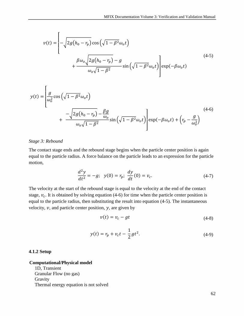
MFIX Documentation Volume 3: Verification and Validation Manual
62
𝑣(𝑡) =
[
−√2𝑔(ℎ0 − 𝑟𝑝) cos (√1 − 𝛽2𝜔𝑜𝑡)
+𝛽𝜔𝑜√2𝑔(ℎ0 − 𝑟𝑝) − 𝑔
𝜔𝑜√1 − 𝛽2sin (√1 − 𝛽2𝜔𝑜𝑡)
]
exp(−𝛽𝜔𝑜𝑡)
(4-5)
𝑦(𝑡) =
[ 𝑔
𝜔𝑜2cos (√1 − 𝛽2𝜔𝑜𝑡)
+ −√2𝑔(ℎ0 − 𝑟𝑝) −
𝛽𝑔𝜔𝑜
𝜔𝑜√1 − 𝛽2sin (√1 − 𝛽2𝜔𝑜𝑡)
]
exp(−𝛽𝜔𝑜𝑡) + (𝑟𝑝 −𝑔
𝜔𝑜2)
(4-6)
Stage 3: Rebound
The contact stage ends and the rebound stage begins when the particle center position is again
equal to the particle radius. A force balance on the particle leads to an expression for the particle
motion,
𝑑2𝑦
𝑑𝑡2= −𝑔; 𝑦(0) = 𝑟𝑝;
𝑑𝑦
𝑑𝑡(0) = 𝑣𝑐 . (4-7)
The velocity at the start of the rebound stage is equal to the velocity at the end of the contact
stage, 𝑣𝑐. It is obtained by solving equation (4-6) for time when the particle center position is
equal to the particle radius, then substituting the result into equation (4-5). The instantaneous
velocity, 𝑣, and particle center position, 𝑦, are given by
𝑣(𝑡) = 𝑣𝑐 − 𝑔𝑡 (4-8)
𝑦(𝑡) = 𝑟𝑝 + 𝑣𝑐𝑡 −1
2𝑔𝑡2. (4-9)
4.1.2 Setup
Computational/Physical model
1D, Transient
Granular Flow (no gas)
Gravity
Thermal energy equation is not solved

MFIX Documentation Volume 3: Verification and Validation Manual
63
Geometry
Coordinate system Cartesian
x-length 1.0 (m)
z-length 1.0 (m)
y-length 1.0 (m)
Solids Properties
Normal spring coefficient, 𝑘𝑛 varied (N·m-1)
Restitution coefficient, 𝑒𝑛 varied ( - )
Friction coefficient, 𝜇 0.0 ( - )
Solids 1 Type DEM
Diameter, 𝑑𝑝 0.2 (m)
Density, 𝜌𝑠 2,600 (kg·m-3)
Boundary Conditions
All boundaries Solid Walls
4.1.3 Results
Simulations of a freely-falling particle dropped from an initial height of 0.5m were conducted for
four particle-wall normal spring coefficients, [1.0, 2.5, 5.0, 10.0] × 104 N·m-1, and five
restitution coefficients, [0.6, 0.7, 0.8, 0.9, 1.0]. The test using a normal spring coefficient of 104
N·m-1 and restitution coefficient 0.6 were unsuccessful because this combination leads to the
particle center crossing the fixed boundary indicating that the particle is located outside of the
domain. The following results were obtained using the Euler time stepping method.
Figure 4-2: Comparison of analytical solution and DEM results for a freely-falling particle using the Euler
time-stepping method for varying restitution coefficient, normal spring coefficient, 𝒌𝒏 = 𝟏𝟎𝟒 N•m-1. (Left)
Particle center position; analytical solutions shown as continuous lines, MFIX-DEM results as points. (Right)
Percent absolute relative error between the analytical and MFIX-DEM particle center positions.
The particle center position for cases using a normal spring coefficient of 104 N·m-1 are shown in
Figure 4-2. These cases demonstrate the largest errors in particle center position during the

MFIX Documentation Volume 3: Verification and Validation Manual
64
contact stage. The large error is attributed to the particle center position approaching the fixed
boundary, 𝑦 → 0, during the contact stage. This leads to near-zero values used in the absolute
value of the relative error calculations. In all other cases, the absolute percent relative error
remains below 3% with errors decreasing with increasing normal spring coefficient.
The particle velocity for cases using a slightly stiffer normal spring coefficient of 105 N·m-1 are
shown in Figure 4-3. Again, the large errors are primarily attributed to near-zero values used in
the relative error calculations. The initial spike in error arises at the peak of the contact stage
when the particle trajectory reverses, passing through zero. Similarly, large relative errors occur
at the peak of the rebound stage when the particle trajectory again reverses direction.
Figure 4-3: Comparison of analytical solution and DEM results for a freely-falling particle using the Euler
time-stepping method for varying restitution coefficients, and normal spring coefficient, 𝒌𝒏 = 𝟏𝟎𝟓 N•m-1. (Left)
Particle velocities; analytical solutions shown as continuous lines, MFIX-DEM results as points. (Right) Percent
absolute relative error between the analytical and MFIX-DEM particle velocities.
Analysis of the time-stepping methods is limited to the free-fall stage and excludes error arising
from the collision model. Pre- and post-collision results using the Euler and Adams-Bashforth
methods with a normal spring coefficient of 105 N·m-1 are shown in Figure 4-3. During the free
fall stage (pre-collision), the Euler method shows a linear accumulation of error in particle
position whereas the error in particle velocity is zero. The Adams-Bashforth method shows no
(zero) error for both particle position and velocity. These results are consistent across all cases.

MFIX Documentation Volume 3: Verification and Validation Manual
65
Figure 4-4: Difference between analytical solution and MFIX-DEM results for a freely-falling particle with
varying restitution coefficient and normal spring coefficient, 𝒌𝒏 = 𝟏𝟎𝟓 N•m-1. Euler method shown as solid line.
Adams-Bashforth method shown as dashed lines. (Left) Difference in particle position. (Right) Difference in
particle velocity.
4.2 DEM02: Bouncing particle
This case provides a comparison between the MFIX-DEM linear spring-dashpot collision model
and the hard sphere model where collisions are instantaneous. The hard sphere model can be
seen as the limiting case where the normal spring coefficient is large, 𝑘𝑛 → ∞. This case was
originally reported in [22].
4.2.1 Description
A smooth (frictionless), spherical particle falls freely under gravity from an initial height, ℎ0, and
bounces upon collision with a fixed wall (see Figure 4-1). Assuming that the collision is
instantaneous, the maximum height the particle reaches after the first collision (bounce), ℎ1max, is
given by
ℎ1max = (ℎ0 − 𝑟𝑝)𝑒𝑛
2 (4-10)
where 𝑟𝑝 is the particle radius, and 𝑒𝑛 is the restitution coefficient. A general expression for the
maximum height following the 𝑘𝑡ℎ bounce is
ℎ𝑘max = (ℎ0 − 𝑟𝑝)𝑒𝑛
2𝑘 + 𝑟𝑝. (4-11)
4.2.2 Setup
Computational/Physical model
1D, Transient
Granular Flow (no gas)
Gravity
Thermal energy equation is not solved

MFIX Documentation Volume 3: Verification and Validation Manual
66
Geometry
Coordinate system Cartesian
x-length 1.0 (m)
z-length 1.0 (m)
y-length 1.0 (m)
Solids Properties
Normal spring coefficient, 𝑘𝑛 varied (N·m-1)
Restitution coefficient, 𝑒𝑛 varied ( - )
Friction coefficient, 𝜇 0.0 ( - )
Solids Type DEM
Diameter, 𝑑𝑝 0.2 (m)
Density, 𝜌𝑠 2,600 (kg·m-3)
Boundary Conditions
All boundaries Solid Walls
4.2.3 Results
Simulations of a freely-falling particle dropped from an initial height of 0.5m were conducted for
three normal spring coefficients, [0.5, 5.0, 50.0] × 105 N·m-1, and six restitution coefficients,
[0.5, 0.6, 0.7, 0.8, 0.9, 1.0]. All simulations employed the Adams-Bashforth time-stepping
method. The maximum height attained after the kth collision for all cases is shown in Figure 4-5.
Figure 4-5: Comparison between the analytic solution from a hard-sphere model (solid lines) and MFIX-
DEM (symbols) of the maximum height reached after the kth wall collision for a freely falling particle. Three
values for the normal spring coefficient are used (left to right) with six restitution coefficients.
Figure 4-6 illustrates the percent relative difference between the analytical solution for a hard-
sphere model and the MFIX-DEM simulation. In the limit of the hard-sphere model (shown left
to right by an increasing spring coefficient), the difference between the two collision models
decreases.

MFIX Documentation Volume 3: Verification and Validation Manual
67
Figure 4-6: Percent relative difference between the analytic solution for a hard-sphere model and MFIX-DEM
of the maximum height reached after the kth wall collision for a freely falling particle. Three values for the
normal spring coefficient are used (left to right) with six restitution coefficients.
4.3 DEM03: Two stacked, compressed particles
This case serves to verify the MFIX-DEM linear spring-dashpot collision model through analysis
of a multi-particle, enduring collision. This test case is based on the work of Chen et al. [21] and
the MFIX-DEM test case was originally reported in [22].
4.3.1 Description
Two particles of equal radius, 𝑟𝑝, are stacked between two fixed walls such that the particles are
compressed. The lower and upper walls are located at 𝑦𝑙 = 0.0 and 𝑦𝑤 = 3.6𝑟𝑝 and the particle
centers are initially located at 𝑦10 = 0.25𝑦𝑤 and 𝑦20 = 0.75𝑦𝑤. This configuration, illustrated in
Figure 4-7, ensures that the particles remain in contact and compressed.
Figure 4-7: Two smooth spherical particles stacked between two fixed walls so that the system is always
under compression. A sketch of the problem mechanics is provided along with force balances for the lower
and upper particles.
An expression for the acceleration of the lower particle (particle 1) is
𝑔
0.25𝑦𝑤
𝑦 0.50𝑦𝑤
𝑦𝑤
0.25𝑦𝑤 𝐹𝑐𝑘
𝐹𝑐𝜂
𝐹𝑤𝐿𝑘
𝐹𝑤𝐿
𝜂
𝑔 𝐹𝑐
𝜂
𝐹𝑐𝑘
𝐹𝑤𝑈
𝜂
𝐹𝑤𝑈𝑘
Lower particle
force balance Upper particle
force balance
1
2

MFIX Documentation Volume 3: Verification and Validation Manual
68
𝑑2𝑦1
𝑑𝑡2= −𝑔 −
𝑘𝑛𝑤
𝑚1(𝑦1 − 𝑟𝑝) −
𝜂𝑛1𝑤
𝑚1
𝑑𝑦1
𝑑𝑡
−𝑘𝑛12
𝑚1(2𝑟𝑝 − (𝑦2 − 𝑦1)) −
𝜂𝑛12
𝑚1(𝑑𝑦1
𝑑𝑡−
𝑑𝑦2
𝑑𝑡)
(4-12)
where 𝑦1 and 𝑦2 are the particle center positions measured from the lower wall, 𝑔 is the
acceleration due to gravity, 𝑘𝑛𝑤 and 𝑘𝑛12 are the particle-wall and particle-particle spring
coefficients, 𝜂𝑛1𝑤 and 𝜂𝑛12 are the particle-wall and particle-particle damping coefficients, and
𝑚1 is the mass of particle 1. Similarly, acceleration of the upper particle (particle 2) is given by
𝑑2𝑦2
𝑑𝑡2= −𝑔 −
𝑘𝑛𝑤
𝑚2(𝑟𝑝 − (𝑦𝑤 − 𝑦2)) −
𝜂𝑛2𝑤
𝑚2
𝑑𝑦2
𝑑𝑡
+𝑘𝑛12
𝑚2(2𝑟𝑝 − (𝑦2 − 𝑦1)) +
𝜂𝑛12
𝑚2(𝑑𝑦1
𝑑𝑡−
𝑑𝑦2
𝑑𝑡)
(4-13)
where 𝜂𝑛2𝑤 is the particle-wall damping coefficient for the upper particle, and 𝑚2 is the mass of
the upper particle.
4.3.2 Setup
Computational/Physical model
1D, Transient
Granular Flow (no gas)
Gravity
Thermal energy equation is not solved
Geometry
Coordinate system Cartesian
x-length 1.0 (m)
z-length 0.0010 (m)
y-length 0.0018 (m)
Solids Properties
Normal spring coefficient, 𝑘𝑛 103 (N·m-1)
Restitution coefficient, 𝑒𝑛 varied ( - )
Friction coefficient, 𝜇 0.0 ( - )
Solids 1 Type DEM
Diameter, 𝑑𝑝1 0.001 (m)
Density, 𝜌𝑠1 20,000 (kg·m-3)
Solids 2 Type DEM
Diameter, 𝑑𝑝2 0.001 (m)

MFIX Documentation Volume 3: Verification and Validation Manual
69
Density, 𝜌𝑠2 10,000 (kg·m-3)
Boundary Conditions
All boundaries Solid Walls
4.3.3 Results
Analytical solutions to equations (4-12) and (4-13) describing the motion of the particles are
readily obtainable for perfectly elastic (𝜂𝑛12 = 𝜂𝑛1𝑤 = 𝜂𝑛2𝑤 = 1.0) particles of equal mass
(𝑚1 = 𝑚2). This is not the case for inelastic particles of different mass, therefore a fourth-order
Runge-Kutta method is used to calculate a secondary numerical solution which is considered to
be the analytical solution during the analysis.
Simulations were conducted for six friction coefficients, [0.5, 0.6, 0.7, 0.8, 0.9, 1.0], using the
Adams-Bashforth time-stepping method. Figure 4-8 shows the motion of the lower (left) and
upper (right) particles as well as the absolute value of the relative error for a restitution
coefficient of 1. The percent relative difference in results remains below 0.1% for this case. This
is the largest observed difference across all cases with the difference in relative error decreasing
with decreasing restitution coefficient.
Figure 4-8: Comparison between the fourth-order Runge-Kutta solution (solid line) and MFIX-DEM
simulation (open symbols) for the center position of two stacked particles compressed between fixed walls for
a restitution coefficient of 1. The absolute percent relative errors are shown as dashed lines.
4.4 DEM04: Slipping on a rough surface
This case serves to verify the MFIX-DEM soft-spring collision model through the analysis of the
rolling friction model. This test case was originally reported in [22].

MFIX Documentation Volume 3: Verification and Validation Manual
70
4.4.1 Description
A spherical particle of radius, 𝑟𝑝, finite translation velocity, 𝑢0, and zero angular velocity, 𝜔0, is
placed on a rough surface as illustrated in Figure 4-9. The particle begins to roll while the
translational velocity decreases because of rolling friction attributed to slip between the particle
and the rough surface at the point of contact (𝑢 ≠ 𝜔𝑟𝑝). The rolling friction converts translation
velocity to angular velocity until there is no slip at the contact point (𝑢 = 𝜔𝑟𝑝). After the no-slip
condition is reached, rolling friction ceases and the particle continues to move with constant
translational and rotational velocities.
Figure 4-9: A spherical particle with finite translational velocity and zero angular velocity is placed on a
rough surface. Forces acting on the particle are indicated.
Kinetic friction is the only translational force acting on the particle and is given by
𝑑𝑢
𝑑𝑡=
𝑑2𝑥
𝑑𝑡2= −𝜇𝑔. (4-14)
where 𝑔 is the acceleration due to gravity, and 𝜇 is the coefficient of friction. Similarly, the
angular velocity is given by
𝑑𝜔
𝑑𝑡=
𝜇𝑔𝑚𝑟𝑝
𝐼 (4-15)
where 𝐼 = 2𝑚𝑟𝑝2/5 and 𝑚 are the particle moment of inertia and mass, respectively. Integrating
equations (4-14) and (4-15) with initial conditions 𝑢0 and 𝜔0, an expression for the time when
rolling friction ceases (𝑢 = 𝜔𝑟𝑝) is obtained,
𝑡𝑠 =2𝑢0
7𝜇𝑔 (4-16)
4.4.2 Setup
Computational/Physical model
1D, Transient
Granular Flow (no gas)
Gravity
Thermal energy equation is not solved
Geometry
𝑔
𝑦
𝑟𝑝 𝐹𝜇
𝜔0
𝑢0
force balance

MFIX Documentation Volume 3: Verification and Validation Manual
71
Coordinate system Cartesian
x-length 1.0 (m)
z-length 1.0 (m)
y-length 1.0 (m)
Solids Properties
Normal spring coefficient, 𝑘𝑛 104 (N·m-1)
Restitution coefficient, 𝑒𝑛 1.0 ( - )
Friction coefficient, 𝜇 varied ( - )
Solids 1 Type DEM
Diameter, 𝑑𝑝 0.001 (m)
Density, 𝜌𝑠 10,000 (kg·m-3)
Boundary Conditions
All boundaries Solid Walls
4.4.3 Results
Simulations were conducted for nine restitution coefficients, [0.2, 0.3, 0.4, 0.4, 0.6, 0.7, 0.8, 0.9
1.0], using the Adams-Bashforth time-stepping method with the results shown in Figure 4-10.
The absolute relative percent error between the MFIX-DEM and analytical value for the non-
dimensionalized time when rolling friction ceases, 𝑡𝑠/(𝜇𝑔/𝑢0), is less than 1% for all reported
conditions. Similarly, the absolute relative percent error between the MFIX-DEM and analytical
value for the non-dimensionalized tangential and angular velocities is less than 0.1% for all
reported conditions. Error between the MFIX-DEM and analytical values can be further reduced
(not shown) by increasing the normal spring coefficient, 𝑘𝑛, which decreases the DEM solids
time-step size.
Figure 4-10: Comparison between the analytical solution (solid line) and MFIX-DEM simulation (open
symbols) of a particle with radius 𝒓𝒑 slipping on a rough surface for various friction coefficients. (left)
Dimensionless slip time end and (right) dimensionless equilibrium tangential, 𝒖, and angular, 𝝎, velocities.

MFIX Documentation Volume 3: Verification and Validation Manual
72
4.5 DEM05: Oblique particle collision
This case serves to verify the normal and tangential components of both the linear spring-dashpot
and Hertzian collision models in MFIX DEM. This case is based on the modeling work of Di
Renzo and Di Maio [23] and utilizes the experimental data of Kharaz, Gorham, and Salman [24].
4.5.1 Description
In the experiments of Kharaz, Gorham, and Salman [24], a spherical particle is dropped from a
fixed height such that it collides with a rigid surface at a known velocity. The angle of the ridged
surface is varied to test impact angles ranging from normal to glancing. The rebound angle, post-
collision angular velocity, and observed tangential restitution coefficient were reported.
In the experiment, the particle strikes an angled anvil as illustrated in Figure 4-11(a). Rather than
modeling an angled surface, the wall is kept level (flat) and the particle is given an initial
trajectory corresponding to the angle found in the experiment as shown in Figure 4-11(b). The
particle is initially positioned close to the wall and gravity is suppressed in the simulations to
eliminate the effects of the rotated geometry with respect to the experimental apparatus.
Figure 4-11: (a) Experimental setup of Kharaz, Gorham, and Salman [24] of a particle striking a fixed, angled
anvil. (b) Simulation setup whereby the particle is given an initial velocity to replicate the particle striking an
angled surface.
4.5.2 Setup
Computational/Physical model
3D, Transient
Granular Flow (no gas)
No gravity
Thermal energy equation is not solved
Geometry
Coordinate system Cartesian
x-length 0.5 (m)
z-length 0.5 (m)
y-length 0.1 (m)
𝑦
𝜃0
𝑦 𝜃𝑟
𝑣0
𝑣𝑟
𝜔𝑟
Rebound Pre-impact
𝑦
𝜃𝑟
𝑣0 𝑣𝑟
𝜔𝑟
Rebound Pre-impact
𝜃0
(a) (b)

MFIX Documentation Volume 3: Verification and Validation Manual
73
Solids Phase 1 DEM
Diameter, 𝑑𝑝 0.005 (m)
Density, 𝜌𝑠 5,000 (kg·m-3)
Solids Phase 2 DEM
Diameter, 𝑑𝑝 0.005 (m)
Density, 𝜌𝑠 5,000 (kg·m-3)
Boundary Conditions
All boundaries No Slip Walls
The mechanical properties for the particle (solids phase 1) and the anvil (solids phase 2 and wall)
are provided for both the linear spring-dashpot and Hertzian collision models. The second solids
phase is given the same properties as the anvil for verification of both the particle-particle and
particle-wall collision model implementations.
Solids Phase 1 Linear Hertzian
Normal spring coefficient, (N·m-
1)
1.72×10⁷ ―
Restitution coefficient, (N·m-1) 1.48×10⁷ ―
Young’s modulus, (Pa) ― 380×109
Poisson ratio ― 0.23
Friction coefficient 0.092 0.092
Solids Phase 2 & Wall
Normal spring coefficient, (N·m-
1)
1.72×10⁷ ―
Restitution coefficient, (N·m-1) 1.48×10⁷ ―
Young’s modulus, (Pa) ― 70×109
Poisson ratio ― 0.25
Friction coefficient 0.092 0.092
4.5.3 Results
Simulations were conducted using the linear spring-dashpot and Hertzian collision models. Each
simulation contained a total of 93 particles. The particle-particle and particle-wall collision
models were tested by varying the initial collision angles between 0 (normal) and 65 degrees
(glancing). Gravity was suppressed in the simulations to eliminate the effects of the rotated
geometry with respect to the experimental apparatus.
The rebound angle, observed tangential restitution coefficient, and post-collision angular velocity
for particle-wall collisions are given in Figure 4-12 with particle-particle collision results shown
in Figure 4-13. There is good agreement between the simulation results and experimental data
for the rebound angle and post-collision angular velocity. Although both models over predict the

MFIX Documentation Volume 3: Verification and Validation Manual
74
observed tangential coefficient for steep (near-normal) collision angles, better agreement is
observed with the linear spring-dashpot model for the parameters used.
Figure 4-12: Particle-wall oblique collision results for the linear spring-dashpot model (solid line), Hertzian
model (dashed line), and experimental data (symbols) of Kharaz, Gorham, and Salman [24].
Figure 4-13: Particle-particle oblique collision results for the linear spring-dashpot model (solid line),
Hertzian model (dashed line), and experimental data (symbols) of Kharaz, Gorham, and Salman [24].
4.6 DEM06: Single particle, terminal velocity
This case investigates the interphase coupling of momentum equations though the gas-solids
drag force. The original case was reported in [22] and has been expanded to test additional
coupling schemes.
4.6.1 Description
A single particle initially at rest is released in a uniform gas stream as illustrated in Figure 4-14
where the gravitational and gas-solids drag forces are the dominant forces acting on the particle.
The velocity of the particle increases until it reaches its terminal velocity where the gravitational
force is equal to the gas-solids drag force.

MFIX Documentation Volume 3: Verification and Validation Manual
75
Figure 4-14: A single spherical particle initially at rest is released in a uniform, vertical air flow. The dominant
forces acting on the particle are the gas-solids drag force, 𝑭𝒅, and the gravitational force, 𝒈.
For a sufficiently small particle, the evolution of the particle velocity is given by
𝑑2𝑦
𝑑𝑡2=
𝑑𝑣𝑝
𝑑𝑡=
𝑔(𝜌𝑝 −𝜌𝑔)
𝜌𝑝−
3
4
𝜌𝑔‖𝑣𝑝 − 𝑣𝑔‖2
𝑑𝑝𝜌𝑝𝐶𝑑; 𝑦(0) = ℎ0;
𝑑𝑦
𝑑𝑡(0) = 0 (4-17)
where 𝑦 is the particle center position measured from the bottom wall, 𝑣𝑝 and 𝑣𝑔 are the particle
and gas velocities, 𝜌𝑝 and 𝜌𝑔 are the particle and gas densities, 𝑑𝑝 is the particle diameter, ℎ0 is
the initial height of the particle, 𝑔 is the acceleration due to gravity, and 𝐶𝑑 is the drag
coefficient. The drag coefficient is estimated here using the Schiller and Naumann [25]
correlation for a single particle in an unbounded medium,
𝐶𝑑 =24
NRe
(1 + 0.15𝑁Re0.687) (4-18)
where 𝑁Re is the Reynolds number based on the slip velocity between the particle and gas
defined as
𝑁Re =𝜌𝑔‖𝑣𝑝 − 𝑣𝑔‖
2𝑑𝑝
𝜇𝑔. (4-19)
4.6.2 Setup
Computational/Physical model
1D, Transient, incompressible
Multiphase flow (gas-solids)
Gravity
Thermal energy equation is not solved
Geometry
Coordinate system Cartesian
x-length 0.01 (m)
z-length 0.10 (m)
y-length 0.01 (m)
Solids Properties
Normal spring coefficient, 𝑘𝑛 10-1 (N·m-1)
𝑣𝑔 𝑔
𝐹𝑑
𝑦

MFIX Documentation Volume 3: Verification and Validation Manual
76
Restitution coefficient, 𝑒𝑛 1.0 ( - )
Friction coefficient, 𝜇 0.0 ( - )
Solids 1 Type DEM
Diameter, 𝑑𝑝 10-4 (m)
Density, 𝜌𝑠 2,000 (kg·m-3)
Boundary Conditions
South face (XZ-plane; y=0.00m) Gas Mass Inflow
Pressure (gauge) 0.00 (Pa)
Gas velocity, 𝑣𝑔 0.40 (m·s-1)
North face (XZ-plane; y=0.10m) Pressure Outflow
Pressure (gauge) 0.00 (Pa)
Top, Bottom, East, West faces Free Slip Walls
4.6.3 Results
A fourth-order Runge-Kutta method was used to calculate the solution to (4-17) which was
subsequently compared with the solutions of the seven MFIX-DEM simulations outlined below.
The first set of simulations were one-way coupled such that only the gas phase volume fraction
was affected by the presence of the particle. Specifically, gas-solids drag force was omitted from
the gas phase momentum equations. This case best captured the above problem description
where a single particle is freely falling through a uniform gas field. In the second group of tests
the gas and solids were fully coupled. Three interpolation methods were used with both the one-
way and fully coupled tests.
Interpolation Scheme Coupling Filter Size
Centroid one-way ―
Garg_2012 one-way ―
DPVM_Square one-way 2.0×10⁻³
Centroid full ―
Garg_2012 full ―
DPVM_Square full 3.0×10⁻³
DPVM_Square full 4.0×10⁻³
Figure 4-15 illustrates a typical comparison of analytical particle velocity evolution over time
obtained by Equation (4-17) and the numerical solution. A comparison of the absolute percent
relative difference between the solutions is shown in Figure 4-16. The numerical solution from
simulations employing one-way coupling (left) compare well with the analytical solution of
Equation (4-17) with the maximum absolute relative difference bounded above by 5 × 10⁻³
percent for the three cases. Additionally, the maximum absolute relative difference for cases with
full coupling is bounded from above by 5 percent.

MFIX Documentation Volume 3: Verification and Validation Manual
77
Figure 4-15: Comparison of the particle velocity evolution obtained by equation (4-17) and MFIX-DEM.
The large difference in results for the fully coupled cases should not be interpreted as error
because the assumption of a uniform gas velocity used to establish Equation (4-17) is no longer
valid when the gas-solids drag is allowed to affect the gas velocity as is the case in the fully
coupled simulations. The suitability of this assumption, or lack thereof, is apparent from
inspecting the results from different coupling schemes. The centroid method concentrates the
gas-solids drag force in the fluid cell containing the particle center. As a result, gas velocity is
impacted the most when compared to the other methods available. The divided particle volume
method (DVPM) diffuses the gas-solids drag force over an area based on the filter width
providing better agreement. Finally, the GARG_2012 scheme shows the best agreement as it
diffuses the gas-solids drag force over the greatest area thereby providing greater consistency
with the uniform flow field assumption.
Figure 4-16: Absolute percent relative difference between particle velocity evolution obtained by equation
(4-17) and MFIX-DEM. (left) Simulations with one-way gas-solids coupling. (right) Fully coupled simulations.

MFIX Documentation Volume 3: Verification and Validation Manual
78
References
[1] AIAA, "Guide for the Verification and Validation of Computational Fluid
Dynamics Simulations (AIAA G-077-1998(2002))," American Institute of
Aeronautics and Astronautics (AIAA), 1998.
[2] P. J. Roache, "Quantification of uncertainty in computational fluid dynamics,"
Annual Review of Fluid Mechanics, vol. 29, pp. 123-160, 1997.
[3] S. Schlesinger, "Terminology for model credibility," SIMULATION, vol. 32, no. 3,
pp. 103-104, 1979.
[4] W. Oberkampf and T. Trucano, "Verification and Validation in Computational
Fluid Dynamics," Sandia National Laboratories, 2002.
[5] P. J. Roache, Fundamentals of Verification and Validation, Socorro, NM: Hermosa
Publishers, 2009.
[6] M. Syamlal, T. O’Brien, S. Benyahia, A. Gel and S. Pannala, "Open-Source
Software in Computational Research: A Case Study," Modelling and Simulation in
Engineering, vol. 937542, 2008.
[7] P. J. Roache and S. Steinberg, "Symbolic manipulation and computational fluid
dynamics," AIAA Journal, vol. 22, no. 10, pp. 1390-1394, October 1984.
[8] C. J. Roy, "Review of code and solution verification procedures for computational
simulation," Journal of Computational Physics, vol. 205, no. 1, pp. 131-156, 2005.
[9] W. L. Oberkampf and C. J. Roy, Verification and validation in scientific
computing, Cambridge: Cambridge University Press, 2010.
[10] W. L. Oberkampf and C. J. Roy, Verification and Validation in Scientific
Computing, New York: Cambridge University Press, 2010.
[11] S. Richards, "Completed Richardson extrapolation in space and time,"
Communications in Nuemerical Methods in Engineering, vol. 13, pp. 573-582,
1997.
[12] A. Choudhary, C. Roy, J. Dietiker, M. Shahnam and R. Garg, "Code Verification
for Multiphase Flows Using the Method of Manufactured Solutions," in ASME
2014 4th Joint US-European Fluids Engineering Division Summer Meeting

MFIX Documentation Volume 3: Verification and Validation Manual
79
collocated with the ASME 2014 12th International Conference on Nanochannels,
Microchannels, and Minichannels, Chicago, Illinois, USA, August 3–7, 2014.
[13] J. M. Vedovoto, A. da Silveira Neto, A. Mura and L. da Silva, "Application of the
method of manufactured solutions to the verification of a pressure-based finite-
volume numerical scheme," Computers & Fluids, vol. 51, no. 1, pp. 85-99, 2011.
[14] R. B. Bond, C. C. Ober, P. M. Knupp and S. W. Bova, "Manufactured Solution for
Computational Fluid Dynamics Boundary Condition Verification," AIAA Journal,
vol. 45, no. 9, pp. 2224-2236, 2007.
[15] A. Choudhary, C. J. Roy, E. A. Luke and S. Veluri, "Code verification of boundary
conditions for compressible and incompressible computational fluid dynamics
codes," Computers and Fluids, In review.
[16] U. Ghia, K. N. Ghia and C. T. Shin, "High-Re solutions for incompressible flow
using the Navier-Stokes equations and a multigrid method," Journal of
Computational Physics, vol. 48, no. 3, pp. 387-411, 1982.
[17] P. M. Gresho and S. T. Chan, "On the theory of semi-implicit projection methods
for viscous incompressible flow and its implementation via a finite element method
that also introduces a nearly consistent mass matrix. Part 2: Implementation,"
International Journal for Numerical Methods in Fluids, vol. 11, no. 5, pp. 621-659,
1990.
[18] R. Liska and B. Wendroff, "Comparison of Several Difference Schemes on 1D and
2D Test Problems for the Euler Equations," SIAM J. Sci. Comput., vol. 25, no. 3,
pp. 995-1017, 2003.
[19] M. Lee and R. D. Moser, "Direct numerical simulation of turbulent channel flow up
to Re_tau = 5200," Journal of Fluid Mechanics, vol. 774, pp. 395-415, 2015.
[20] M. V. Zagarola and A. J. Smits, "Mean Flow Scaling of Turbulent Pipe Flow,"
Journal of Fluid Mechanics, vol. 373, pp. 33-79, 1998.
[21] F. Chen, E. C. Drumm and G. Guiochon, "Prediction/Verification of Particle
Motion in One Dimension with the Discrete-Element Method," International
Journal of Geomechanics, vol. 7, no. 5, p. 344–352, 2007.

MFIX Documentation Volume 3: Verification and Validation Manual
80
[22] R. Garg, J. Galvin, T. Li and S. Pannala, "Open-source MFIX-DEM software for
gas–solids flows: Part I—Verification studies," Powder Technology, vol. 220, pp.
122-137, 2012.
[23] A. Di Renzo and F. P. Di Maio, "Comparison of contact-force models for the
simulation of collisions in DEM-based granular flow codes," Chemical Engineering
Science, vol. 59, no. 3, pp. 525-541, 2004.
[24] A. H. Kharaz, D. A. Gorham and A. D. Salman, "An experimental study of the
elastic rebound of spheres," Powder Technology, vol. 120, no. 3, pp. 281-291,
2001.
[25] L. Schiller and A. Naumann, "Fundamental calculations in gravitational
processing," Zeitschrift Des Vereines Deutscher Ingenieure, vol. 77, pp. 318-320,
1933.
[26] C. J. Roy, C. C. Nelson, T. M. Smith and C. C. Ober, "Verification of Euler/Navier-
Stokes codes using the method of manufactured solutions," International Journal
for Numerical Methods in Fluids, vol. 44, no. 6, pp. 599-620, 2004.
[27] A. Choudhary, "Verification of Compressible and Incompressible Computational
Fluid Dynamics Codes and Residual-based Mesh Adaptation," Ph.D. Dissertation,
Virginia Tech, Blacksburg, 2015.
[28] S. B. Pope, "An Explanation of the Turbulent Round-Jet/Plane-Jet Anomaly," AIAA
Journal, vol. 16, no. 3, 1978.
[29] D. C. Wilcox, Turbulence Modeling for CFD, DCW Industries, 1994.
[30] C. J. Roy, "Grid Convergence Error Analysis for Mixed-Order Numerical
Schemes," AIAA Journal, vol. 41, no. 4, pp. 595-604, 2003.
[31] J. W. Banks, T. Aslam and W. J. Rider, "On sub-linear convergence for linearly
degenerate waves in capturing schemes," Journal of Computational Physics, vol.
227, p. 6985–7002, 2008.

MFIX Documentation Volume 3: Verification and Validation Manual
81
Appendix A: Manufactured Solution Mathematical Forms
(Note: All solution variables are in SI units.)
A.1 Baseline 3D Manufactured Solutions
The baseline manufactured solution selected for the verification study is a combination of sine
and cosine functions and takes the following general form [26, 27]
𝜙(𝑥, 𝑦, 𝑧) = 𝜙0 + 𝜙𝑥𝑓𝜙𝑥 (𝑎𝜙𝑥𝜋𝑥
𝐿) + 𝜙𝑦𝑓𝜙𝑦 (
𝑎𝜙𝑦𝜋𝑦
𝐿) + 𝜙𝑧𝑓𝜙𝑧 (
𝑎𝜙𝑧𝜋𝑧
𝐿)
+ 𝜙𝑥𝑦𝑓𝜙𝑥𝑦 (𝑎𝜙𝑥𝑦𝜋𝑥𝑦
𝐿2) + 𝜙𝑦𝑧𝑓𝜙𝑦𝑧 (
𝑎𝜙𝑦𝑧𝜋𝑦𝑧
𝐿2)
+ 𝜙𝑧𝑥𝑓𝜙𝑧𝑥 (𝑎𝜙𝑧𝑥𝜋𝑧𝑥
𝐿2)
(A-1)
where, 𝐿 is a characteristic length (herein, selected equal to the domain length or 𝐿 = 1), and
𝜙 = [𝑃𝑔, 𝑢𝑔, 𝑣𝑔, 𝑤𝑔, 𝑢𝑠, 𝑣𝑠 , 𝑤𝑠, 𝑇𝑔, 𝑇𝑠]𝑇 represents the set of primitive variables being tested for
order of accuracy. The sinusoidal functions (𝑓𝜙𝑥, 𝑓𝜙𝑦, etc.) selected are shown in the table below
Variable, 𝜙 𝑓𝜙𝑥 𝑓𝜙𝑦 𝑓𝜙𝑧 𝑓𝜙𝑥𝑦 𝑓𝜙𝑦𝑧 𝑓𝜙𝑧𝑥
𝑢𝑔 sin cos cos cos sin cos
𝑣𝑔 sin cos cos cos sin cos
𝑤𝑔 cos sin cos sin sin cos
𝑃𝑔 cos cos sin cos sin cos
𝑇𝑔 cos cos sin cos sin cos
𝑇𝑠 cos cos sin cos sin cos
휀𝑠 cos cos sin -- -- --
The frequency constants (𝑎𝜙𝑥, 𝑎𝜙𝑦, 𝑎𝜙𝑥𝑦, etc.) and the amplitude constants (𝜙0, 𝜙𝑥, 𝜙𝑥𝑦, etc.)
are selected to ensure functions that are smooth but show reasonable periodicity and magnitude
within the domain. The frequency constants selected are shown in the following table.
Variable, 𝜙 𝑎𝜙𝑥 𝑎𝜙𝑦 𝑎𝜙𝑧 𝑎𝜙𝑥𝑦 𝑎𝜙𝑦𝑧 𝑎𝜙𝑧𝑥
𝑢𝑔 0.5 0.85 0.4 0.6 0.8 0.9
𝑣𝑔 0.8 0.8 0.5 0.9 0.4 0.6
𝑤𝑔 0.85 0.9 0.5 0.4 0.8 0.75
𝑃𝑔 0.4 0.45 0.85 0.75 0.7 0.8
𝑇𝑔 0.75 1.25 0.8 0.65 0.5 0.6
𝑇𝑠 0.5 0.9 0.8 0.5 0.65 0.4
휀𝑠 0.4 0.5 0.5 -- -- --

MFIX Documentation Volume 3: Verification and Validation Manual
82
The amplitude constants selected are shown in the following table.
Variable, 𝜙 𝜙0 𝜙𝑥 𝜙𝑦 𝜙𝑧 𝜙𝑥𝑦 𝜙𝑦𝑧 𝜙𝑧𝑥
𝑢𝑔 7 3 -4 -3 2 1.5 2
𝑣𝑔 9 -5 4 5 -3 2.5 3.5
𝑤𝑔 8 -4 3.5 4.2 -2.2 2.1 2.5
𝑃𝑔 100 20 -50 20 -25 -10 10
𝑇𝑔 350 10 -30 20 -12 10 8
𝑇𝑠 300 15 -20 15 -10 12 10
휀𝑠 0.3 0.06 0.1 0.06 -- -- --
A.2 Two-Phase, 3D, Manufactured Solutions
The baseline manufactured solutions presented above are used to generate manufactured
solutions for the two-phase flow test cases. As an example, the manufactured solution for the test
case presented in Section 2.6 is provided next.
The manufactured solutions for the scalar variables (𝑃𝑔, 𝑇𝑔, and 𝑇𝑠) are simply obtained from Eq.
(A-1) and by substituting the appropriate functions and constants described above. For example,
for the pressure variable (𝑃𝑔), this function is as follow:
𝑃𝑔 = 100 + 20 cos(0.4𝜋𝑥) − 50 cos(0.45𝜋𝑦) + 20 sin(0.85𝜋𝑧)
− 25 cos(0.75𝜋𝑥𝑦) − 10 sin(0.7𝜋𝑦𝑧) + 10 cos(0.8𝜋𝑧𝑥)
(A-2)
The manufactured solutions for velocity components of the gas phase are obtained by taking the
curl of the baseline velocity vector field, i.e.,
�⃗� 𝑔 = 𝑢𝑔𝑖̂ + 𝑣𝑔𝑗̂ + 𝑤𝑔�̂� = ||
𝑖̂ 𝑗̂ �̂�𝜕
𝜕𝑥
𝜕
𝜕𝑦
𝜕
𝜕𝑦𝜙(𝑢𝑔) 𝜙(𝑣𝑔) 𝜙(𝑤𝑔)
|| (A-3)
where, for example, 𝜙(𝑢𝑔) is the baseline manufactured solution obtained from Eq. (A-1), the
functions, and the constants described above for the variable 𝑢𝑔. This results in a divergence free
velocity field because ∇ ⋅ (∇ × �⃗⃗� ) is identically zero for any vector field, �⃗⃗� . Thus, the
manufactured solution for 𝑢𝑔 is given as:

MFIX Documentation Volume 3: Verification and Validation Manual
83
𝑢𝑔 = −𝜋𝑦 cos(0.4𝜋𝑦𝑧) + 2.5𝜋 sin(0.5𝜋𝑧) + 2.1𝜋𝑥 sin(0.6𝜋𝑧𝑥)
− 0.88𝜋𝑥 cos(0.4𝜋𝑥𝑦) + 3.15𝜋 cos(0.9𝜋𝑦)
+ 0.68𝜋𝑧 cos(0.8𝜋𝑦𝑧)
(A-4)
Similarly, the manufactured solution for 𝑣𝑔 and 𝑤𝑔 can be derived.
Finally, the manufactured solution for velocity components of the solids phase is selected as
simply the following divergence free field:
𝑢𝑠 = 5 sin2(0.5𝜋(𝑥 + 𝑦 + 𝑧)) (A-5)
𝑣𝑠 = 5 cos2(0.5𝜋(𝑥 + 𝑦 + 𝑧)) (A-6)
𝑤𝑠 = 5 (A-7)
Manufactured solutions for other MMS test cases presented are derived using the baseline
manufactured solutions and appropriate constraints (divergence free field, boundary conditions,
etc.). For a complete look at the MMS function and MMS source terms, please see the
MMS_MOD.f file under the respective test case of the MFIX distribution.
A.3 MMS02 manufactured solutions
The manufactured solutions for the two-phase, 3D, curl-based functions with constant volume
fraction are listed below.
Gas pressure:
𝑝𝑔 = 𝑝𝑔0 + 𝑝𝑔𝑥 cos (𝐴𝑝𝑔𝑥𝜋𝑥) + 𝑝𝑔𝑦 cos (𝐴𝑝𝑔𝑦
𝜋𝑦) + 𝑝𝑔𝑥𝑦 cos (𝐴𝑝𝑔𝑥𝑦𝜋𝑥𝑦)
+ 𝑝𝑔𝑧 sin (𝐴𝑝𝑔𝑧𝜋𝑧) + 𝑝𝑔𝑦𝑧 sin (𝐴𝑝𝑔𝑦𝑧
𝜋𝑦𝑧)
+ 𝑝𝑔𝑧𝑥 cos (𝐴𝑝𝑔𝑧𝑥𝜋𝑧𝑥)
(A-8)
Gas velocity components:
𝑢𝑔 = 𝐴𝑤𝑔𝑦𝜋𝑤𝑔𝑦 cos (𝐴𝑤𝑔𝑦
𝜋𝑦) + 𝐴𝑤𝑔𝑥𝑦𝜋𝑤𝑔𝑥𝑦𝑥 cos (𝐴𝑤𝑔𝑥𝑦
𝜋𝑥𝑦)
− 𝐴𝑣𝑔𝑦𝑧𝜋𝑣𝑔𝑦𝑧𝑦 cos (𝐴𝑣𝑔𝑦𝑧
𝜋𝑦𝑧) + 𝐴𝑤𝑔𝑦𝑧𝜋𝑤𝑔𝑦𝑧𝑧 cos (𝐴𝑤𝑔𝑦𝑧
𝜋𝑦𝑧)
+ 𝐴𝑣𝑔𝑧𝜋𝑣𝑔𝑧 sin (𝐴𝑣𝑔𝑧
𝜋𝑧) + 𝐴𝑣𝑔𝑧𝑥𝜋𝑣𝑔𝑧𝑥𝑥 sin (𝐴𝑣𝑔𝑧𝑥
𝜋𝑧𝑥)
(A-9)

MFIX Documentation Volume 3: Verification and Validation Manual
84
𝑣𝑔 = −𝐴𝑤𝑔𝑥𝑦𝜋𝑤𝑔𝑥𝑦𝑦 cos (𝐴𝑤𝑔𝑥𝑦
𝜋𝑥𝑦) + 𝐴𝑢𝑔𝑦𝑧𝜋𝑢𝑔𝑦𝑧𝑦 cos (𝐴𝑢𝑔𝑦𝑧
𝜋𝑦𝑧)
+ 𝐴𝑤𝑔𝑥𝜋𝑤𝑔𝑥 sin (𝐴𝑤𝑔𝑥
𝜋𝑥) − 𝐴𝑢𝑔𝑧𝜋𝑢𝑔𝑧 sin (𝐴𝑢𝑔𝑧
𝜋𝑧)
− 𝐴𝑢𝑔𝑧𝑥𝜋𝑢𝑔𝑧𝑥𝑥 sin (𝐴𝑢𝑔𝑧𝑥
𝜋𝑧𝑥) + 𝐴𝑤𝑔𝑧𝑥𝜋𝑤𝑔𝑧𝑥𝑧 sin (𝐴𝑤𝑔𝑧𝑥
𝜋𝑧𝑥)
(A-10)
𝑤𝑔 = 𝐴𝑣𝑔𝑥𝜋𝑣𝑔𝑥 cos (𝐴𝑣𝑔𝑥
𝜋𝑥) − 𝐴𝑢𝑔𝑦𝑧𝜋𝑢𝑔𝑦𝑧𝑧 cos (𝐴𝑢𝑔𝑦𝑧
𝜋𝑦𝑧)
+ 𝐴𝑢𝑔𝑦𝜋𝑢𝑔𝑦 sin (𝐴𝑢𝑔𝑦
𝜋𝑦) + 𝐴𝑢𝑔𝑥𝑦𝜋𝑢𝑔𝑥𝑦𝑥 sin (𝐴𝑢𝑔𝑥𝑦
𝜋𝑥𝑦)
− 𝐴𝑣𝑔𝑥𝑦𝜋𝑣𝑔𝑥𝑦𝑦 sin (𝐴𝑣𝑔𝑥𝑦
𝜋𝑥𝑦) − 𝐴𝑣𝑔𝑧𝑥𝜋𝑣𝑔𝑧𝑥𝑧 sin (𝐴𝑣𝑔𝑧𝑥
𝜋𝑧𝑥)
(A-11)
Solids velocity components:
𝑢𝑚 = 𝑢𝑚0 sin2 (𝜋
2(𝑥 + 𝑦 + 𝑧)) (A-12)
𝑣𝑚 = 𝑣𝑚0 cos2 (𝜋
2(𝑥 + 𝑦 + 𝑧)) (A-13)
𝑤𝑚 = 𝑤𝑚0 (A-14)
Gas and solids temperature:
𝑇𝑔 = 𝑇𝑔0 + 𝑇𝑔𝑥 cos (𝐴𝑇𝑔𝑥𝜋𝑥) + 𝑇𝑔𝑦 cos (𝐴𝑇𝑔𝑦
𝜋𝑦) + 𝑇𝑔𝑥𝑦 cos (𝐴𝑇𝑔𝑥𝑦𝜋𝑥𝑦)
+ 𝑇𝑔𝑧 sin (𝐴𝑇𝑔𝑧𝜋𝑧) + 𝑇𝑔𝑦𝑧 sin (𝐴𝑇𝑔𝑦𝑧
𝜋𝑦𝑧) + 𝑇𝑔𝑧𝑥 cos (𝐴𝑇𝑔𝑧𝑥𝜋𝑧𝑥)
(A-15)
𝑇𝑚 = 𝑇𝑚0 + 𝑇𝑚𝑥 cos(𝐴𝑇𝑚𝑥𝜋𝑥) + 𝑇𝑚𝑦 cos (𝐴𝑇𝑚𝑦
𝜋𝑦) + 𝑇𝑚𝑥𝑦 cos (𝐴𝑇𝑚𝑥𝑦𝜋𝑥𝑦)
+ 𝑇𝑚𝑧 sin(𝐴𝑇𝑚𝑧𝜋𝑧) + 𝑇𝑚𝑦𝑧 sin (𝐴𝑇𝑚𝑦𝑧
𝜋𝑦𝑧)
+ 𝑇𝑚𝑧𝑥 cos(𝐴𝑇𝑚𝑧𝑥𝜋𝑧𝑥)
(A-16)
Gas and solids volume fractions:
휀𝑔 = 1 − (휀𝑚0 + 휀𝑚𝑥 cos(𝐴𝜀𝑚𝑥𝜋𝑥) + 휀𝑚𝑦 cos (𝐴𝜀𝑚𝑦
𝜋𝑦)
+ 휀𝑚𝑥𝑦 cos (𝐴𝜀𝑚𝑥𝑦𝜋𝑥𝑦) + 휀𝑚𝑧 sin(𝐴𝜀𝑚𝑧
𝜋𝑧)
+ 휀𝑚𝑦𝑧 sin (𝐴𝜀𝑚𝑦𝑧𝜋𝑦𝑧) + 휀𝑚𝑧𝑥 cos(𝐴𝜀𝑚𝑧𝑥
𝜋𝑧𝑥))
(A-17)

MFIX Documentation Volume 3: Verification and Validation Manual
85
휀𝑚 = 휀𝑚0 + 휀𝑚𝑥 cos(𝐴𝜀𝑚𝑥𝜋𝑥) + 휀𝑚𝑦 cos (𝐴𝜀𝑚𝑦
𝜋𝑦) + 휀𝑚𝑥𝑦 cos (𝐴𝜀𝑚𝑥𝑦𝜋𝑥𝑦)
+ 휀𝑚𝑧 sin(𝐴𝜀𝑚𝑧𝜋𝑧) + 휀𝑚𝑦𝑧 sin (𝐴𝜀𝑚𝑦𝑧
𝜋𝑦𝑧)
+ 휀𝑚𝑧𝑥 cos(𝐴𝜀𝑚𝑧𝑥𝜋𝑧𝑥)
(A-18)
Solids granular temperature:
𝜃𝑚 = 𝜃𝑚0 + 𝜃𝑚𝑥 cos(𝐴𝜃𝑚𝑥𝜋𝑥) + 𝜃𝑚𝑦 cos (𝐴𝜃𝑚𝑦
𝜋𝑦) + 𝜃𝑚𝑥𝑦 cos (𝐴𝜃𝑚𝑥𝑦𝜋𝑥𝑦)
+ 𝜃𝑚𝑧 sin(𝐴𝜃𝑚𝑧𝜋𝑧) + 𝜃𝑚𝑦𝑧 sin (𝐴𝜃𝑚𝑦𝑧
𝜋𝑦𝑧)
+ 𝜃𝑚𝑧𝑥 cos(𝐴𝜃𝑚𝑧𝑥𝜋𝑧𝑥)
(A-19)
The parameters appearing in the manufactured solutions are as follows:
𝑝𝑔0 100.0 𝑣𝑔𝑥 -5.0 𝑤𝑚0 5.0 휀𝑚0 0.3
𝑝𝑔𝑥 20.0 𝑣𝑔𝑦 4.0 𝑇𝑔0 350 휀𝑚𝑥 0.0
𝑝𝑔𝑦 -50.0 𝑣𝑔𝑧 5.0 𝑇𝑔𝑥 10 휀𝑚𝑦 0.0
𝑝𝑔𝑧 20.0 𝑣𝑔𝑥𝑦 -3.0 𝑇𝑔𝑦 -30 휀𝑚𝑧 0.0
𝑝𝑔𝑥𝑦 -25.0 𝑣𝑔𝑦𝑧 2.5 𝑇𝑔𝑧 20 휀𝑚𝑥𝑦 0.0
𝑝𝑔𝑦𝑧 -10.0 𝑣𝑔𝑧𝑥 3.5 𝑇𝑔𝑥𝑦 -12 휀𝑚𝑦𝑧 0.0
𝑝𝑔𝑧𝑥 10.0 𝐴𝑣𝑔𝑥 0.8 𝑇𝑔𝑦𝑧 10 휀𝑚𝑧𝑥 0.0
𝐴𝑝𝑔𝑥 0.4 𝐴𝑣𝑔𝑦
0.8 𝑇𝑔𝑧𝑥 8 𝐴𝜀𝑚𝑥 0.5
𝐴𝑝𝑔𝑦 0.45 𝐴𝑣𝑔𝑧
0.5 𝐴𝑇𝑔𝑥 0.75 𝐴𝜀𝑚𝑦
0.5
𝐴𝑝𝑔𝑧 0.85 𝐴𝑣𝑔𝑥𝑦
0.9 𝐴𝑇𝑔𝑦 1.25 𝐴𝜀𝑚𝑧
0.5
𝐴𝑝𝑔𝑥𝑦 0.75 𝐴𝑣𝑔𝑦𝑧
0.4 𝐴𝑇𝑔𝑧 0.8 𝐴𝜀𝑚𝑥𝑦
0.4
𝐴𝑝𝑔𝑦𝑧 0.7 𝐴𝑣𝑔𝑧𝑥
0.6 𝐴𝑇𝑔𝑥𝑦 0.65 𝐴𝜀𝑚𝑦𝑧
0.4
𝐴𝑝𝑔𝑧𝑥 0.8 𝑤𝑔0 8.0 𝐴𝑇𝑔𝑦𝑧
0.5 𝐴𝜀𝑚𝑧𝑥 0.4
𝑢𝑔0 7.0 𝑤𝑔𝑥 -4.0 𝐴𝑇𝑔𝑧𝑥 0.6 𝜃𝑚0 100.0
𝑢𝑔𝑥 3.0 𝑤𝑔𝑦 3.5 𝑇𝑚0 300 𝜃𝑚𝑥 5.0
𝑢𝑔𝑦 -4.0 𝑤𝑔𝑧 4.2 𝑇𝑚𝑥 15 𝜃𝑚𝑦 -10.0
𝑢𝑔𝑧 -3.0 𝑤𝑔𝑥𝑦 -2.2 𝑇𝑚𝑦 -20 𝜃𝑚𝑧 12.0
𝑢𝑔𝑥𝑦 2.0 𝑤𝑔𝑦𝑧 2.1 𝑇𝑚𝑧 15 𝜃𝑚𝑥𝑦 -8.0
𝑢𝑔𝑦𝑧 1.5 𝑤𝑔𝑧𝑥 2.5 𝑇𝑚𝑥𝑦 -10 𝜃𝑚𝑦𝑧 10.0
𝑢𝑔𝑧𝑥 -2.0 𝐴𝑤𝑔𝑥 0.85 𝑇𝑚𝑦𝑧 12 𝜃𝑚𝑧𝑥 7.0
𝐴𝑢𝑔𝑥 0.5 𝐴𝑤𝑔𝑦
0.9 𝑇𝑚𝑧𝑥 10 𝐴𝜃𝑚𝑥 0.8
𝐴𝑢𝑔𝑦 0.85 𝐴𝑤𝑔𝑧
0.5 𝐴𝑇𝑚𝑥 0.5 𝐴𝜃𝑚𝑦
1.25
𝐴𝑢𝑔𝑧 0.4 𝐴𝑤𝑔𝑥𝑦
0.4 𝐴𝑇𝑚𝑦 0.9 𝐴𝜃𝑚𝑧
0.7

MFIX Documentation Volume 3: Verification and Validation Manual
86
𝐴𝑢𝑔𝑥𝑦 0.6 𝐴𝑤𝑔𝑦𝑧
0.8 𝐴𝑇𝑚𝑧 0.8 𝐴𝜃𝑚𝑥𝑦
0.5
𝐴𝑢𝑔𝑦𝑧 0.8 𝐴𝑤𝑔𝑧𝑥
0.75 𝐴𝑇𝑚𝑥𝑦 0.5 𝐴𝜃𝑚𝑦𝑧
0.6
𝐴𝑢𝑔𝑧𝑥 0.9 𝑢𝑚0 5.0 𝐴𝑇𝑚𝑦𝑧
0.65 𝐴𝜃𝑚𝑧𝑥 0.7
𝑣𝑔0 9.0 𝑣𝑚0 5.0 𝐴𝑇𝑚𝑧𝑥 0.4
A.4 MMS03 manufactured solutions
The manufactured solutions for the two-phase, 3D, curl-based functions with variable volume
fraction are listed below.
Gas pressure:
𝑝𝑔 = 𝑝𝑔0 + 𝑝𝑔𝑥 cos (𝐴𝑝𝑔𝑥𝜋𝑥) + 𝑝𝑔𝑦 cos (𝐴𝑝𝑔𝑦
𝜋𝑦) + 𝑝𝑔𝑥𝑦 cos (𝐴𝑝𝑔𝑥𝑦𝜋𝑥𝑦)
+ 𝑝𝑔𝑧 sin (𝐴𝑝𝑔𝑧𝜋𝑧) + 𝑝𝑔𝑦𝑧 sin (𝐴𝑝𝑔𝑦𝑧
𝜋𝑦𝑧)
+ 𝑝𝑔𝑧𝑥 cos (𝐴𝑝𝑔𝑧𝑥𝜋𝑧𝑥)
(A-20)
Gas velocity components:
𝑢𝑔 =1
휀𝑔[𝐴𝑤𝑔𝑦
𝜋𝑤𝑔𝑦 cos (𝐴𝑤𝑔𝑦𝜋𝑦) + 𝐴𝑤𝑔𝑥𝑦
𝜋𝑤𝑔𝑥𝑦𝑥 cos (𝐴𝑤𝑔𝑥𝑦𝜋𝑥𝑦)
− 𝐴𝑣𝑔𝑦𝑧𝜋𝑣𝑔𝑦𝑧𝑦 cos (𝐴𝑣𝑔𝑦𝑧
𝜋𝑦𝑧) + 𝐴𝑤𝑔𝑦𝑧𝜋𝑤𝑔𝑦𝑧𝑧 cos (𝐴𝑤𝑔𝑦𝑧
𝜋𝑦𝑧)
+ 𝐴𝑣𝑔𝑧𝜋𝑣𝑔𝑧 sin (𝐴𝑣𝑔𝑧
𝜋𝑧) + 𝐴𝑣𝑔𝑧𝑥𝜋𝑣𝑔𝑧𝑥𝑥 sin (𝐴𝑣𝑔𝑧𝑥
𝜋𝑧𝑥)]
(A-21)
𝑣𝑔 =1
휀𝑔[−𝐴𝑤𝑔𝑥𝑦
𝜋𝑤𝑔𝑥𝑦𝑦 cos (𝐴𝑤𝑔𝑥𝑦𝜋𝑥𝑦) + 𝐴𝑢𝑔𝑦𝑧
𝜋𝑢𝑔𝑦𝑧𝑦 cos (𝐴𝑢𝑔𝑦𝑧𝜋𝑦𝑧)
+ 𝐴𝑤𝑔𝑥𝜋𝑤𝑔𝑥 sin (𝐴𝑤𝑔𝑥
𝜋𝑥) − 𝐴𝑢𝑔𝑧𝜋𝑢𝑔𝑧 sin (𝐴𝑢𝑔𝑧
𝜋𝑧)
− 𝐴𝑢𝑔𝑧𝑥𝜋𝑢𝑔𝑧𝑥𝑥 sin (𝐴𝑢𝑔𝑧𝑥
𝜋𝑧𝑥) + 𝐴𝑤𝑔𝑧𝑥𝜋𝑤𝑔𝑧𝑥𝑧 sin (𝐴𝑤𝑔𝑧𝑥
𝜋𝑧𝑥)]
(A-22)
𝑤𝑔 =1
휀𝑔[𝐴𝑣𝑔𝑥
𝜋𝑣𝑔𝑥 cos (𝐴𝑣𝑔𝑥𝜋𝑥) − 𝐴𝑢𝑔𝑦𝑧
𝜋𝑢𝑔𝑦𝑧𝑧 cos (𝐴𝑢𝑔𝑦𝑧𝜋𝑦𝑧)
+ 𝐴𝑢𝑔𝑦𝜋𝑢𝑔𝑦 sin (𝐴𝑢𝑔𝑦
𝜋𝑦) + 𝐴𝑢𝑔𝑥𝑦𝜋𝑢𝑔𝑥𝑦𝑥 sin (𝐴𝑢𝑔𝑥𝑦
𝜋𝑥𝑦)
− 𝐴𝑣𝑔𝑥𝑦𝜋𝑣𝑔𝑥𝑦𝑦 sin (𝐴𝑣𝑔𝑥𝑦
𝜋𝑥𝑦) − 𝐴𝑣𝑔𝑧𝑥𝜋𝑣𝑔𝑧𝑥𝑧 sin (𝐴𝑣𝑔𝑧𝑥
𝜋𝑧𝑥)]
(A-23)

MFIX Documentation Volume 3: Verification and Validation Manual
87
Solids velocity components:
𝑢𝑚 =1
휀𝑚[𝑢𝑚0 sin2 (
𝜋
2(𝑥 + 𝑦 + 𝑧))] (A-24)
𝑣𝑚 =1
휀𝑚[𝑣𝑚0 cos2 (
𝜋
2(𝑥 + 𝑦 + 𝑧))] (A-25)
𝑤𝑚 =1
휀𝑚𝑤𝑚0 (A-26)
Gas and solids temperature:
𝑇𝑔 = 𝑇𝑔0 + 𝑇𝑔𝑥 cos (𝐴𝑇𝑔𝑥𝜋𝑥) + 𝑇𝑔𝑦 cos (𝐴𝑇𝑔𝑦
𝜋𝑦) + 𝑇𝑔𝑥𝑦 cos (𝐴𝑇𝑔𝑥𝑦𝜋𝑥𝑦)
+ 𝑇𝑔𝑧 sin (𝐴𝑇𝑔𝑧𝜋𝑧) + 𝑇𝑔𝑦𝑧 sin (𝐴𝑇𝑔𝑦𝑧
𝜋𝑦𝑧) + 𝑇𝑔𝑧𝑥 cos (𝐴𝑇𝑔𝑧𝑥𝜋𝑧𝑥)
(A-27)
𝑇𝑚 = 𝑇𝑚0 + 𝑇𝑚𝑥 cos(𝐴𝑇𝑚𝑥𝜋𝑥) + 𝑇𝑚𝑦 cos (𝐴𝑇𝑚𝑦
𝜋𝑦) + 𝑇𝑚𝑥𝑦 cos (𝐴𝑇𝑚𝑥𝑦𝜋𝑥𝑦)
+ 𝑇𝑚𝑧 sin(𝐴𝑇𝑚𝑧𝜋𝑧) + 𝑇𝑚𝑦𝑧 sin (𝐴𝑇𝑚𝑦𝑧
𝜋𝑦𝑧)
+ 𝑇𝑚𝑧𝑥 cos(𝐴𝑇𝑚𝑧𝑥𝜋𝑧𝑥)
(A-28)
Solids granular temperature:
𝜃𝑚 = 𝜃𝑚0 + 𝜃𝑚𝑥 cos(𝐴𝜃𝑚𝑥𝜋𝑥) + 𝜃𝑚𝑦 cos (𝐴𝜃𝑚𝑦
𝜋𝑦) + 𝜃𝑚𝑥𝑦 cos (𝐴𝜃𝑚𝑥𝑦𝜋𝑥𝑦)
+ 𝜃𝑚𝑧 sin(𝐴𝜃𝑚𝑧𝜋𝑧) + 𝜃𝑚𝑦𝑧 sin (𝐴𝜃𝑚𝑦𝑧
𝜋𝑦𝑧)
+ 𝜃𝑚𝑧𝑥 cos(𝐴𝜃𝑚𝑧𝑥𝜋𝑧𝑥)
(A-29)
The parameters appearing in the manufactured solutions are as follows:
𝑝𝑔0 100.0 𝑣𝑔𝑥 -5.0 𝑤𝑚0 5.0 휀𝑚0 0.3
𝑝𝑔𝑥 20.0 𝑣𝑔𝑦 4.0 𝑇𝑔0 350 휀𝑚𝑥 0.06
𝑝𝑔𝑦 -50.0 𝑣𝑔𝑧 5.0 𝑇𝑔𝑥 10 휀𝑚𝑦 -0.1
𝑝𝑔𝑧 20.0 𝑣𝑔𝑥𝑦 -3.0 𝑇𝑔𝑦 -30 휀𝑚𝑧 0.06
𝑝𝑔𝑥𝑦 -25.0 𝑣𝑔𝑦𝑧 2.5 𝑇𝑔𝑧 20 휀𝑚𝑥𝑦 0.0
𝑝𝑔𝑦𝑧 -10.0 𝑣𝑔𝑧𝑥 3.5 𝑇𝑔𝑥𝑦 -12 휀𝑚𝑦𝑧 0.0
𝑝𝑔𝑧𝑥 10.0 𝐴𝑣𝑔𝑥 0.8 𝑇𝑔𝑦𝑧 10 휀𝑚𝑧𝑥 0.0
𝐴𝑝𝑔𝑥 0.4 𝐴𝑣𝑔𝑦
0.8 𝑇𝑔𝑧𝑥 8 𝐴𝜀𝑚𝑥 0.4

MFIX Documentation Volume 3: Verification and Validation Manual
88
𝐴𝑝𝑔𝑦 0.45 𝐴𝑣𝑔𝑧
0.5 𝐴𝑇𝑔𝑥 0.75 𝐴𝜀𝑚𝑦
0.5
𝐴𝑝𝑔𝑧 0.85 𝐴𝑣𝑔𝑥𝑦
0.9 𝐴𝑇𝑔𝑦 1.25 𝐴𝜀𝑚𝑧
0.5
𝐴𝑝𝑔𝑥𝑦 0.75 𝐴𝑣𝑔𝑦𝑧
0.4 𝐴𝑇𝑔𝑧 0.8 𝐴𝜀𝑚𝑥𝑦
0.4
𝐴𝑝𝑔𝑦𝑧 0.7 𝐴𝑣𝑔𝑧𝑥
0.6 𝐴𝑇𝑔𝑥𝑦 0.65 𝐴𝜀𝑚𝑦𝑧
0.4
𝐴𝑝𝑔𝑧𝑥 0.8 𝑤𝑔0 8.0 𝐴𝑇𝑔𝑦𝑧
0.5 𝐴𝜀𝑚𝑧𝑥 0.4
𝑢𝑔0 7.0 𝑤𝑔𝑥 -4.0 𝐴𝑇𝑔𝑧𝑥 0.6 𝜃𝑚0 100.0
𝑢𝑔𝑥 3.0 𝑤𝑔𝑦 3.5 𝑇𝑚0 300 𝜃𝑚𝑥 5.0
𝑢𝑔𝑦 -4.0 𝑤𝑔𝑧 4.2 𝑇𝑚𝑥 15 𝜃𝑚𝑦 -10.0
𝑢𝑔𝑧 -3.0 𝑤𝑔𝑥𝑦 -2.2 𝑇𝑚𝑦 -20 𝜃𝑚𝑧 12.0
𝑢𝑔𝑥𝑦 2.0 𝑤𝑔𝑦𝑧 2.1 𝑇𝑚𝑧 15 𝜃𝑚𝑥𝑦 -8.0
𝑢𝑔𝑦𝑧 1.5 𝑤𝑔𝑧𝑥 2.5 𝑇𝑚𝑥𝑦 -10 𝜃𝑚𝑦𝑧 10.0
𝑢𝑔𝑧𝑥 -2.0 𝐴𝑤𝑔𝑥 0.85 𝑇𝑚𝑦𝑧 12 𝜃𝑚𝑧𝑥 7.0
𝐴𝑢𝑔𝑥 0.5 𝐴𝑤𝑔𝑦
0.9 𝑇𝑚𝑧𝑥 10 𝐴𝜃𝑚𝑥 0.8
𝐴𝑢𝑔𝑦 0.85 𝐴𝑤𝑔𝑧
0.5 𝐴𝑇𝑚𝑥 0.5 𝐴𝜃𝑚𝑦
1.25
𝐴𝑢𝑔𝑧 0.4 𝐴𝑤𝑔𝑥𝑦
0.4 𝐴𝑇𝑚𝑦 0.9 𝐴𝜃𝑚𝑧
0.7
𝐴𝑢𝑔𝑥𝑦 0.6 𝐴𝑤𝑔𝑦𝑧
0.8 𝐴𝑇𝑚𝑧 0.8 𝐴𝜃𝑚𝑥𝑦
0.5
𝐴𝑢𝑔𝑦𝑧 0.8 𝐴𝑤𝑔𝑧𝑥
0.75 𝐴𝑇𝑚𝑥𝑦 0.5 𝐴𝜃𝑚𝑦𝑧
0.6
𝐴𝑢𝑔𝑧𝑥 0.9 𝑢𝑚0 5.0 𝐴𝑇𝑚𝑦𝑧
0.65 𝐴𝜃𝑚𝑧𝑥 0.7
𝑣𝑔0 9.0 𝑣𝑚0 5.0 𝐴𝑇𝑚𝑧𝑥 0.4
A.5 MMS04 manufactured solutions
The manufactured solutions for the No-slip wall BC, single phase, 3D, curl-based functions are
listed below.
Gas pressure:
𝑝𝑔 = 𝑝𝑔0 + 𝑝𝑔𝑥 cos (𝐴𝑝𝑔𝑥𝜋𝑥) + 𝑝𝑔𝑦 cos (𝐴𝑝𝑔𝑦
𝜋𝑦) + 𝑝𝑔𝑥𝑦 cos (𝐴𝑝𝑔𝑥𝑦𝜋𝑥𝑦)
+ 𝑝𝑔𝑧 sin (𝐴𝑝𝑔𝑧𝜋𝑧) + 𝑝𝑔𝑦𝑧 sin (𝐴𝑝𝑔𝑦𝑧
𝜋𝑦𝑧)
+ 𝑝𝑔𝑧𝑥 cos (𝐴𝑝𝑔𝑧𝑥𝜋𝑧𝑥)
(A-30)

MFIX Documentation Volume 3: Verification and Validation Manual
89
Gas velocity components:
𝑢𝑔 = 𝑥2 [𝐴𝑤𝑔𝑦𝜋𝑤𝑔𝑦 cos (𝐴𝑤𝑔𝑦
𝜋𝑦) + 𝐴𝑤𝑔𝑥𝑦𝜋𝑤𝑔𝑥𝑦𝑥 cos (𝐴𝑤𝑔𝑥𝑦
𝜋𝑥𝑦)
− 𝐴𝑣𝑔𝑦𝑧𝜋𝑣𝑔𝑦𝑧𝑦 cos (𝐴𝑣𝑔𝑦𝑧
𝜋𝑦𝑧) + 𝐴𝑤𝑔𝑦𝑧𝜋𝑤𝑔𝑦𝑧𝑧 cos (𝐴𝑤𝑔𝑦𝑧
𝜋𝑦𝑧)
+ 𝐴𝑣𝑔𝑧𝜋𝑣𝑔𝑧 sin (𝐴𝑣𝑔𝑧
𝜋𝑧) + 𝐴𝑣𝑔𝑧𝑥𝜋𝑣𝑔𝑧𝑥𝑥 sin (𝐴𝑣𝑔𝑧𝑥
𝜋𝑧𝑥)]
(A-31)
𝑣𝑔 = 𝑥2 [−𝐴𝑤𝑔𝑥𝑦𝜋𝑤𝑔𝑥𝑦𝑦 cos (𝐴𝑤𝑔𝑥𝑦
𝜋𝑥𝑦) + 𝐴𝑢𝑔𝑦𝑧𝜋𝑢𝑔𝑦𝑧𝑦 cos (𝐴𝑢𝑔𝑦𝑧
𝜋𝑦𝑧)
+ 𝐴𝑤𝑔𝑥𝜋𝑤𝑔𝑥 sin (𝐴𝑤𝑔𝑥
𝜋𝑥) − 𝐴𝑢𝑔𝑧𝜋𝑢𝑔𝑧 sin (𝐴𝑢𝑔𝑧
𝜋𝑧)
− 𝐴𝑢𝑔𝑧𝑥𝜋𝑢𝑔𝑧𝑥𝑥 sin (𝐴𝑢𝑔𝑧𝑥
𝜋𝑧𝑥) + 𝐴𝑤𝑔𝑧𝑥𝜋𝑤𝑔𝑧𝑥𝑧 sin (𝐴𝑤𝑔𝑧𝑥
𝜋𝑧𝑥)]
+ 2𝑥 [−𝑤𝑔0 − 𝑤𝑔𝑥 cos (𝐴𝑤𝑔𝑥𝜋𝑥) − 𝑤𝑔𝑧 cos (𝐴𝑤𝑔𝑧
𝜋𝑧)
− 𝑤𝑔𝑧𝑥 cos (𝐴𝑤𝑔𝑧𝑥𝜋𝑧𝑥) − 𝑤𝑔𝑦 sin (𝐴𝑤𝑔𝑦
𝜋𝑦)
− 𝑤𝑔𝑥𝑦 sin (𝐴𝑤𝑔𝑥𝑦𝜋𝑥𝑦) − 𝑤𝑔𝑦𝑧 sin (𝐴𝑤𝑔𝑦𝑧
𝜋𝑦𝑧)]
(A-32)
𝑤𝑔 = 𝑥2 [𝐴𝑣𝑔𝑥𝜋𝑣𝑔𝑥 cos (𝐴𝑣𝑔𝑥
𝜋𝑥) − 𝐴𝑢𝑔𝑦𝑧𝜋𝑢𝑔𝑦𝑧𝑧 cos (𝐴𝑢𝑔𝑦𝑧
𝜋𝑦𝑧)
+ 𝐴𝑢𝑔𝑦𝜋𝑢𝑔𝑦 sin (𝐴𝑢𝑔𝑦
𝜋𝑦) + 𝐴𝑢𝑔𝑥𝑦𝜋𝑢𝑔𝑥𝑦𝑥 sin (𝐴𝑢𝑔𝑥𝑦
𝜋𝑥𝑦)
− 𝐴𝑣𝑔𝑥𝑦𝜋𝑣𝑔𝑥𝑦𝑦 sin (𝐴𝑣𝑔𝑥𝑦
𝜋𝑥𝑦) − 𝐴𝑣𝑔𝑧𝑥𝜋𝑣𝑔𝑧𝑥𝑧 sin (𝐴𝑣𝑔𝑧𝑥
𝜋𝑧𝑥)]
+ 2𝑥 [𝑣𝑔0 + 𝑣𝑔𝑦 cos (𝐴𝑣𝑔𝑦𝜋𝑦) + 𝑣𝑔𝑥𝑦 cos (𝐴𝑣𝑔𝑥𝑦
𝜋𝑥𝑦)
+ 𝑣𝑔𝑧 cos (𝐴𝑣𝑔𝑧𝜋𝑧) + 𝑣𝑔𝑧𝑥 cos (𝐴𝑣𝑔𝑧𝑥
𝜋𝑧𝑥) + 𝑣𝑔𝑥 sin (𝐴𝑣𝑔𝑥𝜋𝑥)
+ 𝑣𝑔𝑦𝑧 sin (𝐴𝑣𝑔𝑦𝑧𝜋𝑦𝑧)]
(A-33)
Gas volume fraction:
휀𝑔 = 1.0 (A-34)
The parameters appearing in the manufactured solutions are as follows:
𝑝𝑔0 100.0 𝑣𝑔0 9.0
𝑝𝑔𝑥 20.0 𝑣𝑔𝑥 -5.0
𝑝𝑔𝑦 -50.0 𝑣𝑔𝑦 4.0
𝑝𝑔𝑧 20.0 𝑣𝑔𝑧 5.0

MFIX Documentation Volume 3: Verification and Validation Manual
90
𝑝𝑔𝑥𝑦 -25.0 𝑣𝑔𝑥𝑦 -3.0
𝑝𝑔𝑦𝑧 -10.0 𝑣𝑔𝑦𝑧 2.5
𝑝𝑔𝑧𝑥 10.0 𝑣𝑔𝑧𝑥 3.5
𝐴𝑝𝑔𝑥 0.4 𝐴𝑣𝑔𝑥
0.8
𝐴𝑝𝑔𝑦 0.45 𝐴𝑣𝑔𝑦
0.8
𝐴𝑝𝑔𝑧 0.85 𝐴𝑣𝑔𝑧
0.5
𝐴𝑝𝑔𝑥𝑦 0.75 𝐴𝑣𝑔𝑥𝑦
0.9
𝐴𝑝𝑔𝑦𝑧 0.7 𝐴𝑣𝑔𝑦𝑧
0.4
𝐴𝑝𝑔𝑧𝑥 0.8 𝐴𝑣𝑔𝑧𝑥
0.6
𝑢𝑔0 7.0 𝑤𝑔0 8.0
𝑢𝑔𝑥 3.0 𝑤𝑔𝑥 -4.0
𝑢𝑔𝑦 -4.0 𝑤𝑔𝑦 3.5
𝑢𝑔𝑧 -3.0 𝑤𝑔𝑧 4.2
𝑢𝑔𝑥𝑦 2.0 𝑤𝑔𝑥𝑦 -2.2
𝑢𝑔𝑦𝑧 1.5 𝑤𝑔𝑦𝑧 2.1
𝑢𝑔𝑧𝑥 -2.0 𝑤𝑔𝑧𝑥 2.5
𝐴𝑢𝑔𝑥 0.5 𝐴𝑤𝑔𝑥
0.85
𝐴𝑢𝑔𝑦 0.85 𝐴𝑤𝑔𝑦
0.9
𝐴𝑢𝑔𝑧 0.4 𝐴𝑤𝑔𝑧
0.5
𝐴𝑢𝑔𝑥𝑦 0.6 𝐴𝑤𝑔𝑥𝑦
0.4
𝐴𝑢𝑔𝑦𝑧 0.8 𝐴𝑤𝑔𝑦𝑧
0.8
𝐴𝑢𝑔𝑧𝑥 0.9 𝐴𝑤𝑔𝑧𝑥
0.75
A.6 MMS05 manufactured solutions
The manufactured solutions for the Free-slip wall BC, single phase, 3D, curl-based functions are
listed below.
Gas pressure:
𝑝𝑔 = 𝑝𝑔0 + 𝑝𝑔𝑥 cos (𝐴𝑝𝑔𝑥𝜋𝑥) + 𝑝𝑔𝑦 cos (𝐴𝑝𝑔𝑦
𝜋𝑦) + 𝑝𝑔𝑥𝑦 cos (𝐴𝑝𝑔𝑥𝑦𝜋𝑥𝑦)
+ 𝑝𝑔𝑧 sin (𝐴𝑝𝑔𝑧𝜋𝑧) + 𝑝𝑔𝑦𝑧 sin (𝐴𝑝𝑔𝑦𝑧
𝜋𝑦𝑧)
+ 𝑝𝑔𝑧𝑥 cos (𝐴𝑝𝑔𝑧𝑥𝜋𝑧𝑥)
(A-35)

MFIX Documentation Volume 3: Verification and Validation Manual
91
Gas velocity components:
𝑢𝑔 = 𝑥3 [𝐴𝑤𝑔𝑦𝜋𝑤𝑔𝑦 cos (𝐴𝑤𝑔𝑦
𝜋𝑦) + 𝐴𝑤𝑔𝑥𝑦𝜋𝑤𝑔𝑥𝑦𝑥 cos (𝐴𝑤𝑔𝑥𝑦
𝜋𝑥𝑦)
− 𝐴𝑣𝑔𝑦𝑧𝜋𝑣𝑔𝑦𝑧𝑦 cos (𝐴𝑣𝑔𝑦𝑧
𝜋𝑦𝑧) + 𝐴𝑤𝑔𝑦𝑧𝜋𝑤𝑔𝑦𝑧𝑧 cos (𝐴𝑤𝑔𝑦𝑧
𝜋𝑦𝑧)
+ 𝐴𝑣𝑔𝑧𝜋𝑣𝑔𝑧 sin (𝐴𝑣𝑔𝑧
𝜋𝑧) + 𝐴𝑣𝑔𝑧𝑥𝜋𝑣𝑔𝑧𝑥𝑥 sin (𝐴𝑣𝑔𝑧𝑥
𝜋𝑧𝑥)]
(A-36)
𝑣𝑔 = 𝑣𝑔0 + 𝑥3 [−𝐴𝑤𝑔𝑥𝑦𝜋𝑤𝑔𝑥𝑦𝑦 cos (𝐴𝑤𝑔𝑥𝑦
𝜋𝑥𝑦) + 𝐴𝑢𝑔𝑦𝑧𝜋𝑢𝑔𝑦𝑧𝑦 cos (𝐴𝑢𝑔𝑦𝑧
𝜋𝑦𝑧)
+ 𝐴𝑤𝑔𝑥𝜋𝑤𝑔𝑥 sin (𝐴𝑤𝑔𝑥
𝜋𝑥) − 𝐴𝑢𝑔𝑧𝜋𝑢𝑔𝑧 sin (𝐴𝑢𝑔𝑧
𝜋𝑧)
− 𝐴𝑢𝑔𝑧𝑥𝜋𝑢𝑔𝑧𝑥𝑥 sin (𝐴𝑢𝑔𝑧𝑥
𝜋𝑧𝑥) + 𝐴𝑤𝑔𝑧𝑥𝜋𝑤𝑔𝑧𝑥𝑧 sin (𝐴𝑤𝑔𝑧𝑥
𝜋𝑧𝑥)]
+ 3𝑥2 [−𝑤𝑔0 − 𝑤𝑔𝑥 cos (𝐴𝑤𝑔𝑥𝜋𝑥) − 𝑤𝑔𝑧 cos (𝐴𝑤𝑔𝑧
𝜋𝑧)
− 𝑤𝑔𝑧𝑥 cos (𝐴𝑤𝑔𝑧𝑥𝜋𝑧𝑥) − 𝑤𝑔𝑦 sin (𝐴𝑤𝑔𝑦
𝜋𝑦)
− 𝑤𝑔𝑥𝑦 sin (𝐴𝑤𝑔𝑥𝑦𝜋𝑥𝑦) − 𝑤𝑔𝑦𝑧 sin (𝐴𝑤𝑔𝑦𝑧
𝜋𝑦𝑧)]
(A-37)
𝑤𝑔 = 𝑤𝑔0 + 𝑥3 [𝐴𝑣𝑔𝑥𝜋𝑣𝑔𝑥 cos (𝐴𝑣𝑔𝑥
𝜋𝑥) − 𝐴𝑢𝑔𝑦𝑧𝜋𝑢𝑔𝑦𝑧𝑧 cos (𝐴𝑢𝑔𝑦𝑧
𝜋𝑦𝑧)
+ 𝐴𝑢𝑔𝑦𝜋𝑢𝑔𝑦 sin (𝐴𝑢𝑔𝑦
𝜋𝑦) + 𝐴𝑢𝑔𝑥𝑦𝜋𝑢𝑔𝑥𝑦𝑥 sin (𝐴𝑢𝑔𝑥𝑦
𝜋𝑥𝑦)
− 𝐴𝑣𝑔𝑥𝑦𝜋𝑣𝑔𝑥𝑦𝑦 sin (𝐴𝑣𝑔𝑥𝑦
𝜋𝑥𝑦) − 𝐴𝑣𝑔𝑧𝑥𝜋𝑣𝑔𝑧𝑥𝑧 sin (𝐴𝑣𝑔𝑧𝑥
𝜋𝑧𝑥)]
+ 3𝑥2 [𝑣𝑔0 + 𝑣𝑔𝑦 cos (𝐴𝑣𝑔𝑦𝜋𝑦) + 𝑣𝑔𝑥𝑦 cos (𝐴𝑣𝑔𝑥𝑦
𝜋𝑥𝑦)
+ 𝑣𝑔𝑧 cos (𝐴𝑣𝑔𝑧𝜋𝑧) + 𝑣𝑔𝑧𝑥 cos (𝐴𝑣𝑔𝑧𝑥
𝜋𝑧𝑥) + 𝑣𝑔𝑥 sin (𝐴𝑣𝑔𝑥𝜋𝑥)
+ 𝑣𝑔𝑦𝑧 sin (𝐴𝑣𝑔𝑦𝑧𝜋𝑦𝑧)]
(A-38)
Gas volume fraction:
휀𝑔 = 1.0 (A-39)
The parameters appearing in the manufactured solutions are as follows:
𝑝𝑔0 100.0 𝑣𝑔0 9.0
𝑝𝑔𝑥 20.0 𝑣𝑔𝑥 -5.0
𝑝𝑔𝑦 -50.0 𝑣𝑔𝑦 4.0
𝑝𝑔𝑧 20.0 𝑣𝑔𝑧 5.0

MFIX Documentation Volume 3: Verification and Validation Manual
92
𝑝𝑔𝑥𝑦 -25.0 𝑣𝑔𝑥𝑦 -3.0
𝑝𝑔𝑦𝑧 -10.0 𝑣𝑔𝑦𝑧 2.5
𝑝𝑔𝑧𝑥 10.0 𝑣𝑔𝑧𝑥 3.5
𝐴𝑝𝑔𝑥 0.4 𝐴𝑣𝑔𝑥
0.8
𝐴𝑝𝑔𝑦 0.45 𝐴𝑣𝑔𝑦
0.8
𝐴𝑝𝑔𝑧 0.85 𝐴𝑣𝑔𝑧
0.5
𝐴𝑝𝑔𝑥𝑦 0.75 𝐴𝑣𝑔𝑥𝑦
0.9
𝐴𝑝𝑔𝑦𝑧 0.7 𝐴𝑣𝑔𝑦𝑧
0.4
𝐴𝑝𝑔𝑧𝑥 0.8 𝐴𝑣𝑔𝑧𝑥
0.6
𝑢𝑔0 7.0 𝑤𝑔0 8.0
𝑢𝑔𝑥 3.0 𝑤𝑔𝑥 -4.0
𝑢𝑔𝑦 -4.0 𝑤𝑔𝑦 3.5
𝑢𝑔𝑧 -3.0 𝑤𝑔𝑧 4.2
𝑢𝑔𝑥𝑦 2.0 𝑤𝑔𝑥𝑦 -2.2
𝑢𝑔𝑦𝑧 1.5 𝑤𝑔𝑦𝑧 2.1
𝑢𝑔𝑧𝑥 -2.0 𝑤𝑔𝑧𝑥 2.5
𝐴𝑢𝑔𝑥 0.5 𝐴𝑤𝑔𝑥
0.85
𝐴𝑢𝑔𝑦 0.85 𝐴𝑤𝑔𝑦
0.9
𝐴𝑢𝑔𝑧 0.4 𝐴𝑤𝑔𝑧
0.5
𝐴𝑢𝑔𝑥𝑦 0.6 𝐴𝑤𝑔𝑥𝑦
0.4
𝐴𝑢𝑔𝑦𝑧 0.8 𝐴𝑤𝑔𝑦𝑧
0.8
𝐴𝑢𝑔𝑧𝑥 0.9 𝐴𝑤𝑔𝑧𝑥
0.75

NETL Technical Report Series
Charles Zeh
Acting Executive Director
Technology Development & Integration Center
National Energy Technology Laboratory
U.S. Department of Energy
Randall Gentry
Deputy Director
Science & Technology Strategic Plans &
Programs
National Energy Technology Laboratory
U.S. Department of Energy
Technology Manager
Strategic Planning
Science & Technology Strategic Plans &
Programs
National Energy Technology Laboratory
U.S. Department of Energy
Bryan Morreale
Executive Director
Research & Innovation Center
National Energy Technology Laboratory
U.S. Department of Energy


![MFIX Documentation Theory Guide [Tech Note] - U.S. Department of](https://static.documents.pub/doc/80x56/61fb0e1c2e268c58cd59a052/mfix-documentation-theory-guide-tech-note-us-department-of.jpg)


