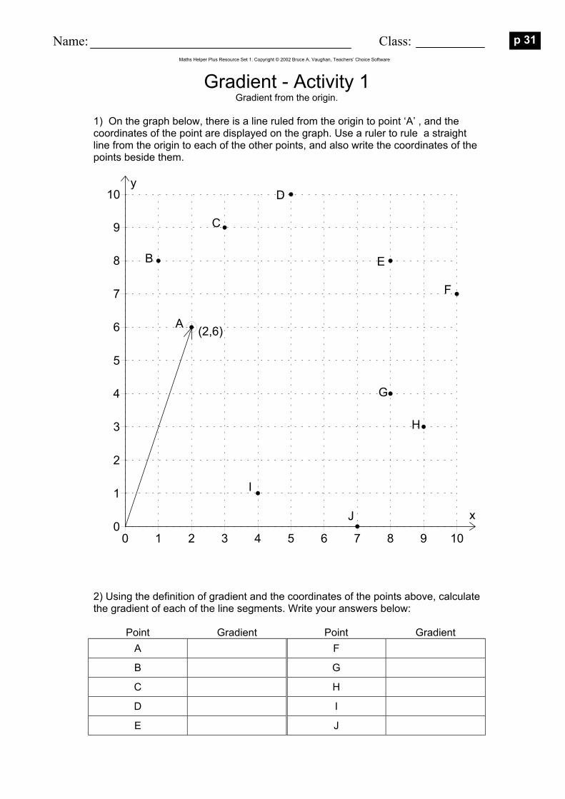
1) On the graph below, there is a line ruled from the origin to point ‘A’ , and the coordinates of the point are displayed on the graph. Use a ruler to rule a straight line from the origin to each of the other points, and also write the coordinates of the points beside them.
x
y
0 1 2 3 4 5 6 7 8 9 100
1
2
3
4
5
6
7
8
9
10
(2,6)A
B
C
D
E
J
I
H
G
F
2) Using the definition of gradient and the coordinates of the points above, calculate the gradient of each of the line segments. Write your answers below:
Point Gradient Point Gradient A F
B G
C H
D I
E J
Use Maths Helper Plus to correct your work. 3) Start Maths Helper Plus and load the ‘Gradient 1.mhp’ document. The graph view will display the graph from question 1 above. 4) Change the coordinates of the ‘probe’ point on the graph to be the same as the point you want to check. The probe point is the second point listed under ‘Probe...’ on the text view. It is already set to the first point, ‘A’: Probe...
(2,6) Probe Click the expand box on the text view to see the value of the gradient, ‘m’, calculated by Maths Helper Plus: Probe...
(2,6)
Linear model 1: y = mx m = 3 ± 0 so: y = 3x
Data box. Expand box
This is the gradient calculated by Maths Helper Plus...
For each point (B to J) click on the data box, change the probe point to the point you want to check, then click outside of the data box. Each time you click outside of the data box, the new gradient will be calculated and displayed.
Name: Class:
Gradient - Activity 2 Gradient of the line segment between two points.
In this activity, you will practice calculating the gradient of the line segment joining two points on the x-y plane. The gradient of the line segment joining points (x1,y1) and (x2,y2) is defined as follows:
12
12
x''in changey''in changegradient
xxyy
−−
==
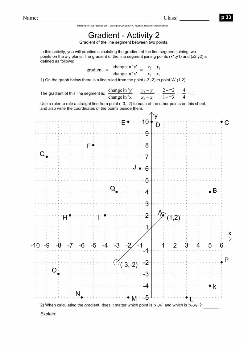
1) On the graph below there is a line ruled from the point (-3,-2) to point ‘A’ (1,2).
The gradient of this line segment is: 144
3122
x''in changey''in change
12
12 ==−−
−−=
−−
=xxyy
Use a ruler to rule a straight line from point (−3,−2) to each of the other points on this sheet, and also write the coordinates of the points beside them.
2) When calculating the gradient, does it matter which point is ‘x1,y1’ and which is ‘x2,y2’ ?
3) Using the definition of gradient and the coordinates of the points above. Complete this table to calculate the gradient of each line segment. (The calculations for point ‘A’ have been done for you): Point x2 x1 x2−x1 y2 y1 y2−y1 Gradient
A 1 -3 4 2 -2 4 1
B -3 -2
C -3 -2
D -3 -2
E -3 -2
F -3 -2
G -3 -2
H -3 -2
I -3 -2
J -3 -2
K -3 -2
L -3 -2
M -3 -2
N -3 -2
O -3 -2
P -3 -2
Q -3 -2
Use Maths Helper Plus to correct your work. 4) Start Maths Helper Plus and load the ‘Gradient 2’ document. The graph view will then display the graph from question 1 above. 5) Change the coordinates of the ‘probe’ point on the graph to be the same as the point you want to check. The probe point is the second point listed under ‘Probe...’ on the text view. (It is already set to the first point, ‘A’.) Click the expand box on the text view to see the value of the gradient, ‘m’, calculated by Maths Helper Plus:
Probe... (-3,-2) (1,2)
Linear model 2: y = mx + c (r = 1) m = 1 ± 0 c = 1 ± 0 so: y = 1x + 1
Probe...
(-3,-2) (1,2) Probe point.
Expand box
This is the gradient calculated by Maths Helper Plus...
Data box. For each point (B to Q) click on the data box, change the probe point to the point you want to check, then click outside of the data box. Each time you click outside of the data box, the new gradient will be calculated and displayed.
Linear Functions - Activity 1 Equation of straight line through points.
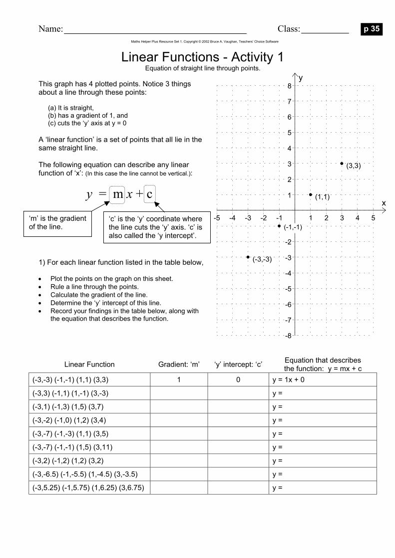
This graph has 4 plotted points. Notice 3 things about a line through these points:
(a) It is straight, (b) has a gradient of 1, and (c) cuts the ‘y’ axis at y = 0
A ‘linear function’ is a set of points that all lie in the same straight line. The following equation can describe any linear function of ‘x’: (In this case the line cannot be vertical.):
y = m x + c 1) For each linear function listed in the table below,
• Plot the points on the graph on this sheet. • Rule a line through the points. • Calculate the gradient of the line. • Determine the ‘y’ intercept of this line. • Record your findings in the table below, along with
the equation that describes the function.
x
y
-5 -4 -3 -2 -1 1 2 3 4 5
-8
-7
-6
-5
-4
-3
-2
-1
1
2
3
4
5
6
7
8
(-3,-3)
(-1,-1)
(1,1)
(3,3)
(-1,-1) ‘m’ is the gradient of the line.
‘c’ is the ‘y’ coordinate where the line cuts the ‘y’ axis. ‘c’ is also called the ‘y intercept’.
Linear Function Gradient: ‘m’ ‘y’ intercept: ‘c’ Equation that describes the function: y = mx + c
(-3,-3) (-1,-1) (1,1) (3,3) 1 0 y = 1x + 0
(-3,3) (-1,1) (1,-1) (3,-3) y =
(-3,1) (-1,3) (1,5) (3,7) y =
(-3,-2) (-1,0) (1,2) (3,4) y =
(-3,-7) (-1,-3) (1,1) (3,5) y =
(-3,-7) (-1,-1) (1,5) (3,11) y =
(-3,2) (-1,2) (1,2) (3,2) y =
(-3,-6.5) (-1,-5.5) (1,-4.5) (3,-3.5) y =
(-3,5.25) (-1,5.75) (1,6.25) (3,6.75) y =
Use Maths Helper Plus to correct your answers to question 1 above. 2) Start Maths Helper Plus and load the ‘Linear Functions 1’ document. The graph view will then display the graph from question 1, above. 3) Follow the instructions below to check each of your linear function equations and correct any errors. The ‘Test equation...’ data set will tell you if your equations are correct. If you type in an equation of a linear function, the points making up the function will plot on the graph view. If the plotted points aren’t the same as the ones you plotted on this sheet, then your equation is wrong and you must correct your mistake.
IMPORTANT: • Do not include the ‘y =’ part of your equation.
So to test the equation: ‘y = 1x + 0’ you only type ‘1x + 0’
• ONLY replace the expression between the last comma and the right bracket. (Shown inside the dotted rectangle below.) If you change other things the equation tester will not work.
FOR THE INTERESTED ‘<-3,3,2>’ creates ‘x’ values from -3 to 3 in steps of 2, thus: -3,-1,1,3
So (<-3,3,2>,1x+0) creates these points: (-3,3) (-1,-1) (1,1) (3,3) and you can see them plotted on the graph view. Only as a last resort and if you can’t work out the equation for a set of points, use the ‘Get equation from points...’ data set, like this:
Test equation...
(<-3,3,2>, 1x+0 ) • • •
Linear model 2: y = mx + c (r = 1) m = 1 ± 0 c = 0 ± 0 so: y = 1x + 0
To test an equation, Click on the data box Type data you want to test. Click outside of the data box.
Get equation from points...
(-3,-3) (-1,-1) (1,1) (3,3)
Linear model 2: y = mx + c (r = 1) m = 1 ± 0 c = 0 ± 0 so: y
To find the equation of the line through a set of points,
Click on the data box Type your points. Click outside of the data box.
= 1x + 0
• • •
This is the equation of the line through the points.
Only trust the answer if these two numbers are both zero, otherwise the points probably aren’t in a straight line.
Linear Functions - Activity 2 An investigation of gradient in linear functions.
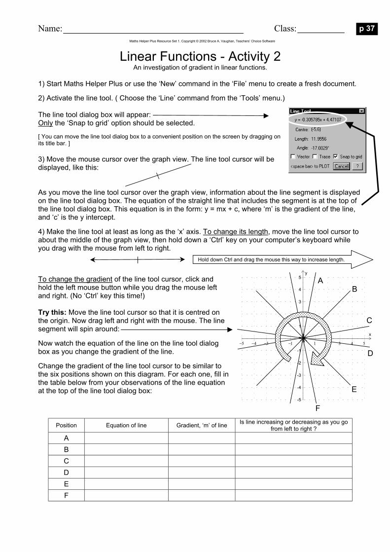
1) Start Maths Helper Plus or use the ‘New’ command in the ‘File’ menu to create a fresh document. 2) Activate the line tool. ( Choose the ‘Line’ command from the ‘Tools’ menu.) The line tool dialog box will appear: Only the ‘Snap to grid’ option should be selected. [ You can move the line tool dialog box to a convenient position on the screen by dragging on its title bar. ] 3) Move the mouse cursor over the graph view. The line tool cursor will be displayed, like this: As you move the line tool cursor over the graph view, information about the line segment is displayed on the line tool dialog box. The equation of the straight line that includes the segment is at the top of the line tool dialog box. This equation is in the form: y = mx + c, where ‘m’ is the gradient of the line, and ‘c’ is the y intercept. 4) Make the line tool at least as long as the ‘x’ axis. To change its length, move the line tool cursor to about the middle of the graph view, then hold down a ‘Ctrl’ key on your computer’s keyboard while you drag with the mouse from left to right. To change the gradient of the line tool cursor, click and hold the left mouse button while you drag the mouse left and right. (No ‘Ctrl’ key this time!) Try this: Move the line tool cursor so that it is centred on the origin. Now drag left and right with the mouse. The line segment will spin around: Now watch the equation of the line on the line tool dialog box as you change the gradient of the line. Change the gradient of the line tool cursor to be similar to the six positions shown on this diagram. For each one, fill in the table below from your observations of the line equation at the top of the line tool dialog box:
Hold down Ctrl and drag the mouse this way to increase length.
x
y
−5 −4 −3 −2 −1 1 2 3 4 5
-5
-4
-3
-2
-1
1
2
3
4
5 A B
C
D
E
F
Position Equation of line Gradient, ‘m’ of line Is line increasing or decreasing as you go from left to right ?
A B C D E F
5) From what you have now observed about gradients of lines, match the gradient values on the left with the statements on the right. Link each matching value and statement with a pencil line.
• m = 0 • m = 35 • m = 0.35 • m = -100 • m = -0.25 • m = 1
• steep line increasing left to right • nearly horizontal line decreasing slightly left to right • very steep line decreasing left to right • horizontal line • 45º line increasing from left to right • nearly horizontal line increasing slightly from left to right
Use the line tool to correct your answers above. Fix up any mistakes. 6) Move the line tool cursor to several different positions on the Maths Helper Plus graph view without pressing any keys or mouse buttons. Look at the line equation displayed in the line tool dialog box while moving the cursor. Does the value of ‘m’ change? 7) You will now investigate this further by plotting some lines with the line tool.
• With the line tool cursor anywhere on the graph grid, press the space bar on your computer keyboard. This will plot the straight line equation.
• Without changing the gradient of the line tool cursor, move it to another position on the graph grid and press the space bar again.
• Repeat until you have plotted about 20 lines, all with the same gradient. Now complete this statement about lines with the same gradient:
“Lines with the same gradient are ________________ “
• Change the line tool gradient to a different value, then plot another 20 lines with the new gradient.
8) What is the greatest possible gradient that a linear function can have?
Linear Functions - Activity 3 An investigation of the ‘y’ intercept of linear functions. [ Assumes knowledge from LF activity 2 ]
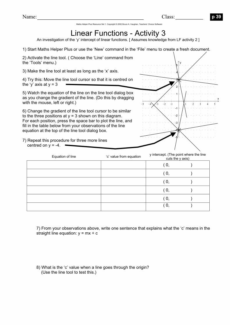
1) Start Maths Helper Plus or use the ‘New’ command in the ‘File’ menu to create a fresh document. 2) Activate the line tool. ( Choose the ‘Line’ command from the ‘Tools’ menu.) 3) Make the line tool at least as long as the ‘x’ axis. 4) Try this: Move the line tool cursor so that it is centred on the ‘y’ axis at y = 3 5) Watch the equation of the line on the line tool dialog box as you change the gradient of the line. (Do this by dragging with the mouse, left or right.) 6) Change the gradient of the line tool cursor to be similar to the three positions at y = 3 shown on this diagram. For each position, press the space bar to plot the line, and fill in the table below from your observations of the line equation at the top of the line tool dialog box. 7) Repeat this procedure for three more lines
x
y
−5 −4 −3 −2 −1 1 2 3 4 5
-5
-4
-3
-2
-1
1
2
3
4
5
centred on y = -4.
Equation of line ‘c’ value from equation y intercept. (The point where the line cuts the y axis)
( 0, )
( 0, )
( 0, )
( 0, )
( 0, ) ( 0, )
7) From your observations above, write one sentence that explains what the ‘c’ means in the straight line equation: y = mx + c 8) What is the ‘c’ value when a line goes through the origin? (Use the line tool to test this.)
INTENTIONALLY BLANK PAGE
Name: Class:
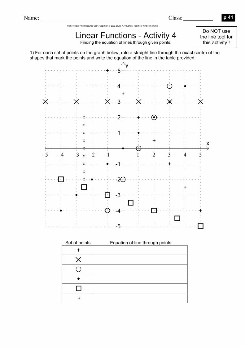
Linear Functions - Activity 4 Finding the equation of lines through given points.
1) For each set of points on the graph below, rule a straight line through the exact centre of the shapes that mark the points and write the equation of the line in the table provided.
x
y
−5 −4 −3 −2 −1 1 2 3 4 5
-5
-4
-3
-2
-1
1
2
3
4
5
Set of points Equation of line through points
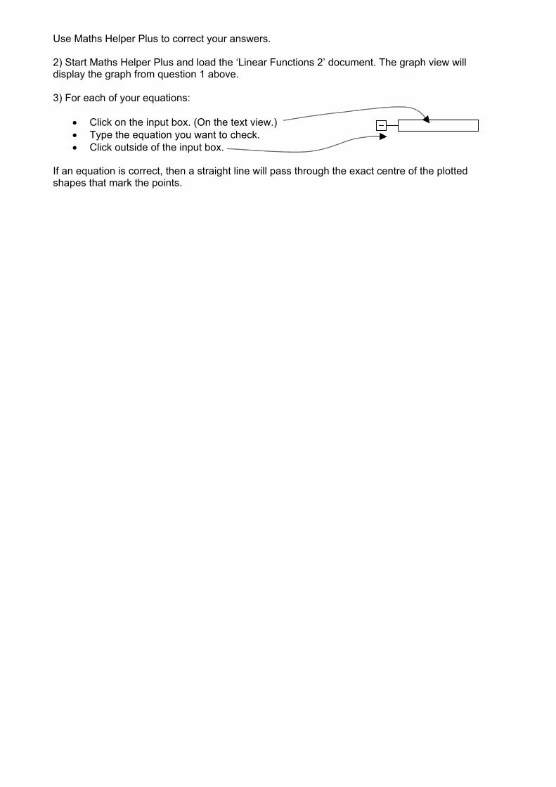
Use Maths Helper Plus to correct your answers. 2) Start Maths Helper Plus and load the ‘Linear Functions 2’ document. The graph view will display the graph from question 1 above. 3) For each of your equations:
• Click on the input box. (On the text view.) • Type the equation you want to check. • Click outside of the input box.
If an equation is correct, then a straight line will pass through the exact centre of the plotted shapes that mark the points.
Name: Class:
Linear Functions - Activity 5 A simple modelling exercise: gradients on Mt Fuji.
1) Start Maths Helper Plus and load the ‘Linear Functions 3’ document. The graph view will display a picture of Mt Fuji:
2) This cross section of Mt Fuji can be approximated by three straight lines:
A C
B
From the graph, estimate the gradient and ‘y’ intercept of linear functions that will closely approximate A, B and C, and hence predict the equation of the segments. Write these in the table below:
Segment: Gradient, m: ‘y’ intercept, c Equation, y = mx + c: A
B
C 3) The Maths Helper Plus text view for this exercise has linear functions already entered for segments A, B and C, all with the equation: y = x. Change these to the equations you wrote in the table above. To change and equation you:
• Click here • Replace ‘y=x’ with your own equation
A) Linear Function 1
y = x • Click here
4) Make adjustments to ‘m’ and ‘c’ values you entered until the equations match the shape of the mountain as much as possible. Write your refined values below:
Segment: Gradient, m: ‘y’ intercept, c Equation, y = mx + c: A
B
C 5) Can linear functions accurately define the shape of Mt Fuji? Explain: OPTIONAL - Restrict the domain of the three linear functions... 6) The ‘domain’ of a function is the set of ‘x’ values for which it is defined. You can restrict the domain of your three linear functions so that they only plot along the outline of the mountain. To define the domain of a plotted function in Maths Helper Plus, carefully point to a graph line and double click. Click on the check box: ‘Restrict domain of plot...’ to select that option. In the ‘from x=’ box, type the leftmost ‘x’ value for the domain. In the ‘to x=’ box, type the rightmost ‘x’ value of the domain. Click OK to close.
INTENTIONALLY BLANK PAGE
Name: Class:
Simultaneous Solutions - Activity 1 Linear Functions.
1) Start Maths Helper Plus and load the document: ‘Simultaneous Solutions 1.mhp’. This document displays two plotted function lines and two data tables:
2) The tables list 11 ordered pairs (x,y) that satisfy each function. What is the one ordered pair that satisfies both functions ?
( , ) An ordered pair that satisfies two functions is called a ‘simultaneous solution’ of the functions. 3) Plot the simultaneous solution on the graph on this sheet. Describe the location of this point relative to the two function graphs.
4) For each of the pairs of linear functions in the table below: a) Hide the graph view. Hold down the ‘Ctrl’ key and press ‘T’ to view the text view only. b) Type one of the functions in the data box for F1 and the other for F2.
c) Examine the tables of ordered pairs that satisfy the functions, then write the simultaneous solution point (x,y) in the table below.
d) Plot this ordered pair with a pencil on the graph on the other side of this sheet. e) Sketch the two linear function graphs on the graph grid on the other side of this sheet. Use only the information in the tables of ordered pairs on the text view. f) Write the coordinates of the intersection point of the graphs in the table below. g) Correct your graph plots. Hold down the ‘Ctrl’ key and press ‘G’ to display the graph view.
Linear Functions Simultaneous Solution (x,y) Intersection point (x,y)
y = 3x + 4, y = x + 4
y = −2x − 5, y = 2x − 1
y = 4x − 7, y = −2x + 5
y = x + 3, y = 3x + 5
y = 2x + 4, y = 3x + 8 5) How can you find simultaneous solutions of equations from a graph ? 6) After looking at the tables and graphs of the linear functions: y = 2x − 1 and y = 2x + 3, explain why they have no simultaneous solutions. 7) How could you know whether or not linear functions have simultaneous solutions just by looking at the equations? (Without seeing the graphs.) 8) Can two linear functions have more than one simultaneous solution? ( Examine y = 2x + 1 and 2y = 4x + 2 )
Simultaneous Solutions - Activity 2 Linear functions and quadratic functions.
1) Start Maths Helper Plus and load the document: ‘Simultaneous Solutions 2.mhp’. This document displays two plotted function graphs and two data tables:
2) The tables list 11 ordered pairs (x,y) that satisfy each function. What are the two ordered pairs that satisfy both functions ?
( , ) and ( , ) An ordered pair that satisfies two functions is called a ‘simultaneous solution’ of the functions. 3) Plot the simultaneous solutions on the graph on this sheet. Describe the location of these points relative to the two function graphs.
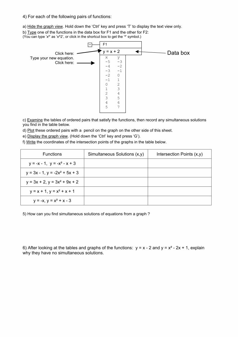
4) For each of the following pairs of functions: a) Hide the graph view. Hold down the ‘Ctrl’ key and press ‘T’ to display the text view only. b) Type one of the functions in the data box for F1 and the other for F2: (You can type ’x²’ as ‘x^2’, or click in the shortcut box to get the ‘²’ symbol.)
c) Examine the tables of ordered pairs that satisfy the functions, then record any simultaneous solutions you find in the table below. d) Plot these ordered pairs with a pencil on the graph on the other side of this sheet. e) Display the graph view. (Hold down the ‘Ctrl’ key and press ‘G’). f) Write the coordinates of the intersection points of the graphs in the table below.
y = -x, y = x² + x - 3 5) How can you find simultaneous solutions of equations from a graph ? 6) After looking at the tables and graphs of the functions: y = x - 2 and y = x² - 2x + 1, explain why they have no simultaneous solutions.


![Mhp Gold The Automated Mhp Mgr[1].Revised](https://static.documents.pub/doc/80x56/55c343e3bb61ebe9438b45a3/mhp-gold-the-automated-mhp-mgr1revised-55c4568e3551f.jpg)


