Michael Gedalin - Purdue Department of Physics and ...lyutikov/phys670/Gedalinplasma.pdf ·...

Lecture Notes in PhysicsIntroduction to Plasma Physics

Michael Gedalin

ii

Contents

1 Basic definitions and parameters 11.1 What is plasma . . . . . . . . . . . . . . . . . . . . . . . . . . . . . . 11.2 Debye shielding . . . . . . . . . . . . . . . . . . . . . . . . . . . . . . 21.3 Plasma parameter . . . . . . . . . . . . . . . . . . . . . . . . . . . . . 41.4 Plasma oscillations . . . . . . . . . . . . . . . . . . . . . . . . . . . . 51.5 ∗Ionization degree∗ . . . . . . . . . . . . . . . . . . . . . . . . . . . . 51.6 Summary . . . . . . . . . . . . . . . . . . . . . . . . . . . . . . . . . 61.7 Problems . . . . . . . . . . . . . . . . . . . . . . . . . . . . . . . . . 7

2 Plasma description 92.1 Hierarchy of descriptions . . . . . . . . . . . . . . . . . . . . . . . . . 92.2 Fluid description . . . . . . . . . . . . . . . . . . . . . . . . . . . . . 102.3 Continuity equation . . . . . . . . . . . . . . . . . . . . . . . . . . . . 102.4 Motion (Euler) equation . . . . . . . . . . . . . . . . . . . . . . . . . 112.5 State equation . . . . . . . . . . . . . . . . . . . . . . . . . . . . . . . 122.6 MHD . . . . . . . . . . . . . . . . . . . . . . . . . . . . . . . . . . . 122.7 Order-of-magnitude estimates . . . . . . . . . . . . . . . . . . . . . . 142.8 Summary . . . . . . . . . . . . . . . . . . . . . . . . . . . . . . . . . 142.9 Problems . . . . . . . . . . . . . . . . . . . . . . . . . . . . . . . . . 15

3 MHD equilibria and waves 173.1 Magnetic field diffusion and dragging . . . . . . . . . . . . . . . . . . 173.2 Equilibrium conditions . . . . . . . . . . . . . . . . . . . . . . . . . . 183.3 MHD waves . . . . . . . . . . . . . . . . . . . . . . . . . . . . . . . . 193.4 Alfven and magnetosonic modes . . . . . . . . . . . . . . . . . . . . . 223.5 Wave energy . . . . . . . . . . . . . . . . . . . . . . . . . . . . . . . . 233.6 Summary . . . . . . . . . . . . . . . . . . . . . . . . . . . . . . . . . 243.7 Problems . . . . . . . . . . . . . . . . . . . . . . . . . . . . . . . . . 24

iii

CONTENTS

4 MHD discontinuities 274.1 Stationary structures . . . . . . . . . . . . . . . . . . . . . . . . . . . 274.2 Discontinuities . . . . . . . . . . . . . . . . . . . . . . . . . . . . . . 284.3 Shocks . . . . . . . . . . . . . . . . . . . . . . . . . . . . . . . . . . . 294.4 Why shocks ? . . . . . . . . . . . . . . . . . . . . . . . . . . . . . . . 314.5 Problems . . . . . . . . . . . . . . . . . . . . . . . . . . . . . . . . . 32

5 Two-fluid description 335.1 Basic equations . . . . . . . . . . . . . . . . . . . . . . . . . . . . . . 335.2 Reduction to MHD . . . . . . . . . . . . . . . . . . . . . . . . . . . . 345.3 Generalized Ohm’s law . . . . . . . . . . . . . . . . . . . . . . . . . . 355.4 Problems . . . . . . . . . . . . . . . . . . . . . . . . . . . . . . . . . 36

6 Waves in dispersive media 376.1 Maxwell equations for waves . . . . . . . . . . . . . . . . . . . . . . . 376.2 Wave amplitude, velocity etc. . . . . . . . . . . . . . . . . . . . . . . . 386.3 Wave energy . . . . . . . . . . . . . . . . . . . . . . . . . . . . . . . . 406.4 Problems . . . . . . . . . . . . . . . . . . . . . . . . . . . . . . . . . 44

7 Waves in two-fluid hydrodynamics 477.1 Dispersion relation . . . . . . . . . . . . . . . . . . . . . . . . . . . . 477.2 Unmagnetized plasma . . . . . . . . . . . . . . . . . . . . . . . . . . . 497.3 Parallel propagation . . . . . . . . . . . . . . . . . . . . . . . . . . . . 497.4 Perpendicular propagation . . . . . . . . . . . . . . . . . . . . . . . . 507.5 General properties of the dispersion relation . . . . . . . . . . . . . . . 517.6 Problems . . . . . . . . . . . . . . . . . . . . . . . . . . . . . . . . . 52

8 Kinetic theory 538.1 Distribution function . . . . . . . . . . . . . . . . . . . . . . . . . . . 538.2 Kinetic equation . . . . . . . . . . . . . . . . . . . . . . . . . . . . . . 548.3 Relation to hydrodynamics . . . . . . . . . . . . . . . . . . . . . . . . 558.4 Waves . . . . . . . . . . . . . . . . . . . . . . . . . . . . . . . . . . . 558.5 Landau damping . . . . . . . . . . . . . . . . . . . . . . . . . . . . . 568.6 Problems . . . . . . . . . . . . . . . . . . . . . . . . . . . . . . . . . 59

9 Micro-instabilities 619.1 Beam (two-stream) instability . . . . . . . . . . . . . . . . . . . . . . 61

10 ∗Nonlinear phenomena∗ 63

A Plasma parameters 65

iv

Preface

v

CONTENTS

vi

Chapter 1

Basic definitions and parameters

In this chapter we learn in what conditions a new state of matter - plasma - appears.

1.1 What is plasma

Plasma is usually said to be a gas of charged particles. Taken as it is, this definition isnot especially useful and, in many cases, proves to be wrong. Yet, two basic necessary(but not sufficient) properties of the plasma are: a) presence of freely moving chargedparticles, and b) large number of these particles. Plasma does not have to consists ofcharged particles only, neutrals may be present as well, and their relative number wouldaffect the features of the system. For the time being, we, however, shall concentrate onthe charged component only.

Large number of charged particles means that we expect that statistical behavior ofthe system is essential to warrant assigning it a new name. How large should it be ?Typical concentrations of ideal gases at normal conditions aren ∼ 1019cm−3. Typicalconcentrations of protons in the near Earth space aren ∼ 1 − 10cm−3. Thus, ionizingonly a tiny fraction of the air we should get a charged particle gas, which is more densethan what we have in space (which is by every lab standard a perfect vacuum). Yet wesay that the whole space in the solar system is filled with a plasma. So how come thatso low density still justifies using a new name, which apparently implies new features ?

A part of the answer is the properties of the interaction. Neutrals as well as chargedparticles interact by means of electromagnetic interactions. However, the forces be-tween neutrals are short-range force, so that in most cases we can consider two neutralatoms not affecting one another until they collide. On the other hand, eachchargedpar-ticle produces a long-range field (like Coulomb field), which can affect many particles ata distance. In order to get a slightly deeper insight into the significance of the long-rangefields, let us consider a gas of immobile (for simplicity) electrons, uniformly distributedinside an infinite cone, and try to answer the question: which electrons affect more the

1

CHAPTER 1. BASIC DEFINITIONS AND PARAMETERS

one which is in the cone vertex ? Roughly speaking, the Coulomb force acting on thechosen electron from another one which is at a distancer, is inversely proportional tothe distance squared,fr ∼ 1/r2. Since the number of electrons which are at this dis-tance,Nr ∝ r2, the total force,Nrfr ∼ r0, is distance independent, which means thatthat electrons which are very far away are of equal importance as the electrons which arevery close. In other words, the chosenprobeexperiences influence from a large numberof particles or the whole system. This brings us to the first hint:collectiveeffects maybe important for a charged particle gas to be able to be called plasma.

1.2 Debye shielding

In order to proceed further we should remember that, in addition to the densityn, everygas has a temperatureT , which is the measure of the random motion of the gas particles.Consider a gas of identical charged particles, each with the chargeq. In order thatthis gas not disperser immediately we have to compensate the charge densitynq withcharges of the opposite sign, thus making the systemneutral. More precisely, we have toneutralize locally, so that the positive chargedensityshould balance the negative chargedensity. Now let us add a test chargeQ which make slight imbalance. We are interestedto know what would be the electric potential induced by this test charge. In the absenceof plasma the answer is immediate:φ = Q/r, wherer is the distance from the chargeQ. Presence of a large number of charged particles, which can move freely, changesthe situation drastically. Indeed, it is immediately clear that the charges of the signopposite toQ, are attracted to the test charge, while the charges of the same sign arerepelled, so that there will appear an opposite charge density in the near vicinity of thetest charge, which tends to neutralize this charge in some way. If the plasma particleswere not randomly moving due to the temperature, they would simply stick to the testparticle thus making it "neutral". Thermal motion does not allow them to remain all thetime nearQ, so that the neutralization cannot be expected to be complete. Nevertheless,some neutralization will occur, and we are going to study it quantitatively.

Before we proceed further we have to explain what electric field is affected. If wemeasure the electric field in the nearest vicinity of any particle, we would recover thesingle particle electric field (Coulomb potential for an immobile particle or Lienard-Viechert potentials for a moving charge), since the influence of other particles is weak.Moreover, since all particles move randomly, the electric field in any point in space willvary very rapidly with time. Taking into account that the number of plasma chargesproducing the electric field is large, we come to the conclusion that we are interested inthe electric field which is averaged over time interval large enough relative to the typicaltime scale of the microscopic field variations, and over volume large enough to includelarge number of particles. In other words, we are interested in the statistically averaged,or self-consistentelectric potential.

2


Establishing the statistical (or average) nature of the electric field around the testcharge we are able now to use the Poisson equation

∆φ = −4πρ− 4πQδ(r), (1.1)

where the last term describes the test point charge in the coordinate origin, whileρ isthe charge density of the plasma particles,

ρ = q(n− n0). (1.2)

Heren is the density of the freely moving charges in the presence of the test charge,while n0 is their density in the absence of this charge. Assuming that the plasma isin thermodynamic equilibrium, we have to conclude that the charged particle are dis-tributed according to the Boltzmann law

n = n0 exp(−U/T ), (1.3)

whereU = qφ. Strictly speaking, the potential in the Boltzmann law should be the local(non-averaged) potential, and averaging

〈exp(−qφ/T )〉 6= exp(−q〉φ〉/T ).

However, sufficiently far from the test charge, whereqφ/T 1 we may Taylor expand

〈exp(−qφ/T )〉 = 1− 〈qφT〉

so that

ρ = −n0q2

Tφ, (1.4)

where nowφ is the self-consistent potential we are looking for. Substituting into (1.1),one gets

1

r2

d

drr2 d

drφ =

4πn0q2

Tφ (1.5)

for r > 0 and boundary conditions readφ → Q/r whenr → 0, andφ → 0 whenr →∞. The above equation can be rewritten as follows:

d2

dr2(rφ) =

1

r2D

(rφ), (1.6)

whererD =

√T/4πn0q2 (1.7)

is called Debye radius. The solution (with the boundary conditions taken into account)is

φ =Q

rexp(−r/rD). (1.8)

3


We see that forr rD the potential is almost not influenced by the plasma particlesand is the Coulomb potentialφ ≈ Q/r. However, atr > rD the potential decreasesexponentially, that is, faster than any power. We say that the plasma charges effectivelyscreen out the electric field of the test charge outside of the Debye spherer = rD.The phenomenon is called Debye screening or shielding, and is our first encounter withthe collective features of the plasma. Indeed, the plasma particles act together, in acoordinated way, to reduce the influence of the externally introduced charge. It is clearthat this effect can be observed only if Debye radius is substantially smaller than thesize of the system,rD L. This is one of the necessary conditions for a gas of chargedparticle to become plasma.

It is worth reminding that the found potential is the potential averaged over spatialscales much large than the mean distance between the particles, and over times muchlarger than the typical time of the microscopic field variations. These variations (calledfluctuations) can be observed and are rather important for plasmas’ life. We won’tdiscuss them in our course.

The two examples of the collective behavior of the plasma (Debye shielding andplasma oscillations) show one more important thing: the plasma particles are "con-nected" one to another viaself-consistentelectromagnetic forces. The self-consistentelectromagnetic fields are the "glue" which makes the plasma particles behave in a co-ordinated way and this is what makes plasma different from other gases.

1.3 Plasma parameter

Since the derived screened potential should be produced in a statistical way by manycharges, we must require that the number of particles inside the Debye sphere be large,ND ∼ nr3

D 1. The parameterg = 1/ND is often called the plasm parameter. We seethat the conditiong 1 is necessary to ensure that a gas of charged particles behavecollectively, thus becoming plasma.

We can arrive at the same parameter in a different way. The average potential energyof the interaction between two charges of the plasma isU ∼ q2/r, wherer is the meandistance between the particles. The latter can be estimated from the condition that thethere is exactly particle in the sphere with the radiusr: nr3 ∼ 1, so thatr ∼ n−1/3. Theaverage kinetic energy of a plasma particle is nothing butT , so that

U

K∼ q2n1/3

T∼ 1

n2/3r2D

= g2/3. (1.9)

If g 1, as it should be for a plasma, then the average potential energy is substantiallysmaller than the average kinetic energy of a particle. In fact, we could expect that sincein order that the charges be able to move freely, the interaction with other particlesshould not be too binding. IfU/K 1, the plasma is said to be ideal, otherwise it is

4


non-ideal. We see that only ideal plasmas are plasma indeed, otherwise the substance ismore like a charged fluid with typical liquid properties.

1.4 Plasma oscillations

In the analysis of the Debye screening the plasma was assumed to be in the equilibrium,that is, the plasma charges were not moving (except for the fast random motion which isaveraged out). Thus, the screening is an example of thestaticcollective behavior. Herewe are going to study an example of thedynamiccollective behavior.

Let us assume that the plasma consists of freely moving electrons and an immobileneutralizing background. Let the charge of the electron beq, massm, and densityn. Letus assume that, for some reason, all electrons, which were in the half-spacex > 0, moveto the distanced to the right, leaving a layer of the non-neutralized background with thecharge densityρ = −nq and widthd. The electric field, produced by this layer on theelectrons onboth edgesis E = 2πρd = −2πnqd (for the electrons at the right edge) andE = 2πρd = 2πnqd (for the electrons at the left edge). The forceF = qE = −2πnq2daccelerates the electrons at the right edge to the left, while the electrons at the left edgeexperience similar acceleration to the right. The relative acceleration of the electrons atthe right and left edges would bea = 2(qE/m) = −4πnq2d/m. On the other hand,a = d, so that one has

d = −ω2pd, ω2

p = 4πnq2/m. (1.10)

The derived equation describes oscillations with theplasma frequencyωp. It should beemphasized that the motion is caused by the coordinated movement of many particlestogether and is thus a purely collective effect. In order to be able to observe theseoscillations their period should be much smaller than the typical life time of the system.

1.5 ∗Ionization degree∗

A plasma does not have to consist only of electrons, or only of electrons and protons.In other words, neutral particles may well be present. In fact, most laboratory plasmasare only partially ionized. They are obtained by breaking neutral atoms into positivelycharged ions and negatively charged electrons. The relative number of ions and atoms,ni/na, is called the degree of ionization. In general, it depends very much on what ismaking ionization. However, in the simplest case of the thermodynamic equilibriumthe ionization degree should depend only on the temperature. Indeed, the process ifionization-recombination,a ↔ i + e, is a special case of a chemical reaction (from thepoint of view of thermodynamics and statistical mechanics). LetI be the ionization

5


potential, that is, the energy needed to separate electron from an atom. Then

ni

na

=gi+e

ga

exp(−I/T ), (1.11)

wheregi+e = gige andga are the number of possible states for the ion+electron andatom, respectively. Usuallyga ∼ gi ∼ 1. However,ge is large. It can be calculatedprecisely but we shall make a simple estimate to illustrate the methods, which are widelyused in plasma physics. The number of available states for an electronge ∼ ∆V ∆3p/h3,where∆V is the volume available for one electron,∆3p is the volume in the momentaspace, andh is the Planck constant. It is obvious that∆V ∼ 1/ne. The volume in themomenta space can be estimated if we remember that the typical kinetic energy of athermal particle,p2/m ∼ T , from which∆3p ∼ (Tme)

3/2. Eventually,

ge ∼(Tme)

3/2

neh3, (1.12)

and (1.11) takes the following form:

nine

na

∼ (Tme)3/2

h3exp(−I/T ). (1.13)

Let us proceed further by assuming that the ions are singly ionized, which givesni = ne,and introduce the total densityn = na + ni and the ionization degreez = ni/n, thenone has

z2

1− z∼ (Tme)

3/2

nh3exp(−I/T ). (1.14)

When the density is low, the pre-exponential in (1.14) is large, and even forT < I theionization degreez may be close to unity,1−z 1. In this case we say that the plasmais fully ionized. The expression (1.14) in its precise form is called Saha formula.

1.6 Summary

• Plasma is a gas of ionized particles.

• Debye length (single species):rD = (T/4πnq2)1/2.

• Debye screening of a test particle:φ = Q exp(−r/rD)/r.

• Plasma parameter:g = 1/nr3D 1.

• Plasma frequency (single species):ωp = (4πnq2/m)1/2.

6


1.7 Problems

PROBLEM 1.1. Calculate the Debye length for a multi-species plasma:ns, qs, Ts. The plasmais quasi-neutral:

∑s nsqs = 0.

PROBLEM 1.2. Calculate the plasma frequency for a multi-species plasma:ns, qs, ms. Theplasma is quasi-neutral:

∑s nsqs = 0.

PROBLEM 1.3. CalculaterD, g andωp for the plasmas in Table A.

PROBLEM 1.4. A parallel plate capacitor charged to±σ is immersed into an electron plasma(immobile ions). What is the potential distribution inside the capacitor ? What is its capacity ?

7


8

Chapter 2

Plasma description

In this chapter we learn about possible methods of plasma description, and derive thepowerful but limited MHD.

2.1 Hierarchy of descriptions

In order to deal with plasma we have to choose some method of description. The moststraightforward and most complete would seem to use the motion equations for all par-ticles together with the Maxwell equations for the electromagnetic fields. However, it isimpossible as well as unreasonable for a many-particle system with a collective behav-ior. A less precise but much more efficient description would be to describe all particlesof the same species as a fluid in the phase space(r, p). This would correspond to theassumption that on average behavior of each particle is the same and independent ofother particles, following only the prescriptions of the self-consistent fields. In this ap-proach we forget about the possible influence of the deviations of the fields from theself-consistent values (fluctuations) and direct (albeit weak) dependence of a particle onits neighbors (correlations). This is the so-called kinetic description.

The further step toward even greater simplification of the plasma description wouldbe to average over momenta for each species, so that only average values remain. Inthis case each speciess is described by the local densityns, local fluid velocityvs, localtemperatureTs or pressureps. This is the so-called multi-fluid description.

Finally, we can even forget that there are different species and describe the plasmaas one fluid with the mass densityρm, velocity V , and pressurep. It is clear thatelectromagnetic field should be added in some way. The rest of the chapter devotedto the description of plasma as a single fluid. The description is known as magneto-hydrodynamics (MHD) for the reasons which become clear later.

9

CHAPTER 2. PLASMA DESCRIPTION

2.2 Fluid description

In order to describe a fluid we choose a physically infinitesimal volumedV surroundingthe pointr in the momentt. The physically infinitesimal volume should be large enoughto contain a large number or particles, so that statistical averaging is possible. On theother hand, it should be small enough to not make the averaging too coarse. With-out coming into details we shall assume that qualitative meaning of this "infinitesimal"volume is sufficiently clear and we can make such choice.

The fluid massρm density is simply the sum of the masses of all particles insidethis volume divided by the volume itself,ρ =

∑mi/dV . Since the result may be

different for volumes chosen in different places or at different times, the density can, ingeneral, depend onr andt. The hydrodynamical velocity of this infinitesimal volumeis simply the velocity of its center of mass:V =

∑mivi/ρdV . Again,V = V (r, t).

Pressure is produced by the random thermal motion of particles (relative to the center-of-mass) in the infinitesimal volume. In order to avoid unnecessary complications weshall assume that the pressure is isotropic, that is, described by a single scalar functionp(r, t). In what follows we shall consider plasma as an ideal gas, that is,p = nT ,wheren(r, t) is the concentration andT (r, t) is the temperature. Thus, we have fourfields: ρm(r, t), V (r, t), p(r, t), andT (r, t), for which we have to find the appropriateevolution equations, connecting the spatial and temporal variations. For brevity we donot write the dependence(r, t) in what follows.

2.3 Continuity equation

We start with the derivation of the continuity equation which is nothing but the massconservation. Let us consider some volume. The total mass inside the volume is

M =

∫V

ρmdV ρm (2.1)

This mass can change only due to the flow of particles into and out of the volume. Ifwe consider a small surface element,dS = ndS, then the mass flow across this surfaceduring timedt will be dM = ρmV dt ·dS. The total flow across the surfaceS enclosingthe volumeV from inside to outside would be

dJ =

∮S

ρmV · dSdt =

∫V

div(ρmV )dV dt (2.2)

Since the flow outward results in the mass decrease, we write

d

dt

∫V

ρmdV = −∫

V

div(ρmV )dV ⇒ (2.3)

10


∫V

[∂ρm

∂t+ div(ρmV )

]dV = 0 ⇒ (2.4)

∂ρm

∂t+ div(ρmV ) = 0. (2.5)

The last relation follows from the fact that the previous should be valid for any arbitrary(including infinitesimal) volume at any time. Equation (2.5) is the continuity equation.

2.4 Motion (Euler) equation

The single particle motion equation is nothing but the equation for the change of itsmomentum. We shall derive the equation of motion for the fluid considering the changeof the momentum of the fluid in some volumeV . The total momentum at any timewould be

P =

∫V

ρmV dV (2.6)

The momentum changes due to the flow of the fluid across the boundary and due to theforces acting from the other fluid at the boundary. Let us start with the momentum flow.The fluid volume which flows across the surfacedS during timedt is V dt · dS. Thisflowing volume takes with it the momentumdP = (ρmV )(V dt · dS). Thus, the totalflow of the momentum outward is

dP =

∮S

(ρmV )(V · dS)dt (2.7)

The total force which acts on the boundaries of the volume from the outside fluid is

F = −∮

S

pdS (2.8)

Combining (2.6)-(2.8) we get

d

dt

∫V

ρmV dV = −∮

S

(ρmV )(V · dS)−∮

S

pdS (2.9)

Further derivation is simpler if we write (2.9) in the component (index) representation:∫V

∂

∂t(ρmVi)dV = −

∮S

(ρmViVj)dSj −∮

S

pδijdSj (2.10)

and use the vector analysis theorem:∮S

AijdSj =

∫V

∂

∂xj

AijdV (2.11)

11


Now we get the motion equation in the following form:

∂

∂t(ρmVi) +

∂

∂xj

(ρmViVj) = − ∂

∂xj

p (2.12)

If we recall that the continuity equation can be written as

∂

∂tρm

∂

∂xj

(ρmVj) = 0 (2.13)

we can rewrite (2.12) in the following widely used form:

ρm

(∂

∂tV + (V ·∇)V

)= − grad p (2.14)

One has to be cautious with the form of the equation since(V · ∇)V is not a goodvector form and cannot be easily written in curvilinear coordinates. Instead one has touse the proper vector representation

(V ·∇)V = grad

(V 2

2

)− V × rot V (2.15)

It is worth noting that the force− grad p thevolumeforce, that is, the forth per unitvolume. If other volume forces exist we should simply add them to the right hand sideof (2.14).

2.5 State equation

We have derived 4 equations (one for the scalar and three for the vector equation) for5 variables:ρm, three components ofV , andp. Therefore, we need another equationfor the pressurep. Either we have to derive it from the first principles, as we did for thecontinuity equation and the motion equation, or to use some sort of approximate closure.For this course we just assume that the pressure is a function of density,p = p(ρ).

2.6 MHD

So far we have been treating a single fluid, without any relation to plasma. What makesthe fluid plasma is its ability to carry currents. If the current density in the plasmais j then it experiences the Ampere force(1/c)j × B, once the magnetic fieldB ispresent. In principle, electric volume forceρqE may be also present. However, in thenon-relativistic MHD approximation the plasma is quasi-neutral and this term is absent,and for the rest of the chapter we do not write the indexm for ρ - it is always the mass

12


density. (If you ever wish to learnrelativistic MHD do not forget the electric force.)Thus, the motion equation takes the following form:

ρ

(∂

∂tV + (V ·∇)V

)= − grad p +

1

cj ×B (2.16)

However, now we have two more vector variables:j and B. It is time to add theMaxwell equations:

div B = 0, (2.17)

rot B =4π

cj +

1

c

∂

∂tE, (2.18)

rot E = −1

c

∂

∂tB. (2.19)

We do not need thediv E = 4πρq equation since quasi-neutrality is assumed and thisequation does not add to the dynamic evolution equations, but rather allows to checkthe assumption in the end of calculations. Eq. (2.17) is a constraint, not an evolutionequation since it does not include time derivative. It is also redundant since (2.19) showsthat once(∂ div B/∂t) = 0, and once (2.17) is satisfied initially it will be satisfiedforever.

It can be shown (we shall see that later in the course) that non-relativistic MHD isthe limit of slow motions and large scale spatial derivatives, so that the displacementcurrent is always negligible, and (2.18) becomes a relation between the magnetic fieldand current density

j =c

4πrot B. (2.20)

The only evolution equation which remains is the induction equation (2.19). However,it includes now the new variableE which does not seem to be otherwise related toany other variable. Ohm’s law comes to help. The local Ohm’s law for a immobileconductor is written asj = σE. Plasma is a moving conductor and the Ohm’s lawshould be written in the plasma rest frame,j ′ = σE′. For non-relativistic flows the restframe electric fieldE′ = E + V ×B/c, while j ′ = j because of the quasi-neutralitycondition. Thus, the Ohm’s law should be written in our case as

j = σ(E + V ×B/c). (2.21)

This relation is used to express the electric field in terms of the magnetic field:

E = −1

cV ×B +

c

4πσrot B, (2.22)

and substitute this in (2.19):

∂

∂tB = rot(V ×B) +

c2

4πσ∆B, (2.23)

13


thus getting an equation containing onlyB andV .Now, substituting (2.20) into (2.16) we get the equation of motion free of the current:

ρ

(∂

∂tV + (V ·∇)V

)= − grad p +

1

4πrot B ×B. (2.24)

2.7 Order-of-magnitude estimates

LetL be the typical inhomogeneity length, which means that when we move by∆x, y, z ∼L the variable under consideration, sayB changes by∆B ∼ B. Now substitute(∂B/∂x) ∼ ∆B/∆x ∼ B/L, that is∇ ∼ 1/L. Similarly, if T is the typical vari-ation time, we have(∂/∂t) ∼ 1/T . Typical velocity then is estimated asV ∼ L/T .Using these definitions we can estimate from the induction equationE ∼ (V/c)B. Re-spectively, the ratio of the displacement current torot B term will be

|1c

∂E

∂t|/| rot B| ∼ LE

cTB∼(

V

c

)2

and is very small for nonrelativistic velocities. This is the reason, why it is usuallyneglected.

For the charge density we haveρq = div E/4π ∼ E/4πL. Thus, the ratio of theelectric and magnetic forces

|ρqE||(1/c)j ×B|

∼ 1

4π

(V

c

)2

and is also negligible.

2.8 Summary

Let us write down again the complete set of the MHD equations:

∂

∂tρ + div(ρV ) = 0, (2.25)

ρd

dtV = − grad p +

1

4πrot B ×B, (2.26)

∂

∂tB = rot(V ×B) +

c2

4πσ∆B, (2.27)

where we introduced the substantial derivative

d

dt=

∂

∂t+ (V ·∇). (2.28)

14


The MHD set should be completed with the state equationp = p(ρ) and is usuallycompleted with the Ohm’s lawE + V ×B/c = j/σ. Whenσ →∞ the MHD is idealMHD.

2.9 Problems

PROBLEM 2.1. Complete the MHD equations for the case when there is gravity.

PROBLEM 2.2. For p ∝ ργ and no entropy change show that the internal energy per unitvolumeu = p/(γ − 1).

PROBLEM 2.3. Derive the energy conservation:

∂

∂t

(12ρV 2 + u +

B2

8π

)+ div

((12ρV 2 + u + p)V +

14π

B × (V ×B))

= 0 (2.29)

PROBLEM 2.4. Let a plasma penetrate a neutral fluid. Discuss the form of the frictional forcebetween the two fluids in the equation of motion for the plasma.

15


16

Chapter 3

MHD equilibria and waves

In this chapter we become familiar with the coordinated behavior of plasma and mag-netic field, and discover the most important features of the plasma - waves.

3.1 Magnetic field diffusion and dragging

We start our study of MHD applications with the analysis of (2.27). Let us considerfirst the case where the plasma is not moving at all, that is,V = 0. Fot simplicity letB = B(x, t)z, so that one gets

∂

∂tB =

c2

4πσ

∂2

∂x2B. (3.1)

Let us represent the magnetic field using Fourier-transform:

B(x, t) =

∫ ∞

−∞B(k, t) exp(ikx)dk, (3.2)

then one has˙

B(k, t) = −k2c2

4πσ˜B(k, t) (3.3)

with the solution˜B(k, t) = ˜B(k, 0) exp(−k2c2t/4πσ). (3.4)

The wavenumberk is the measure of spatial inhomogeneity: the largerk the smalleris the inhomogeneity scale. Eq. (3.4) shows that the inhomogeneous magnetic fielddisappears with time, and the rate of disappearance higher for the components withsmaller scales of inhomogeneity. This phenomenon is known as the magnetic fielddiffusion and is responsible for the graduate dissipation of the magnetic fields in stars.

Let us no consider the opposite case:σ → ∞ andV 6= 0. Let us choose a closedpath (contour)L moving with the plasma and calculate the change of the magnetic flux

17

CHAPTER 3. MHD EQUILIBRIA AND WAVES

across the surfaceS enclosed by this contour,Φ =∫

SB · dS. The flux changes due to

the local change of the magnetic field and due to the change of the contour moving withthe plasma. The total change during the timedt is

dΦ =

∫S

∂B

∂t· dSdt +

∮L

B · (V dt× dL)

=

(∫S

∂B

∂t· dS −

∮L

(V ×B) · dL

)dt

=

∫S

(∂B

∂t− rot(V ×B)

)· dSdt = 0

that is, the magnetic flux across the contour moving with the plasma, does not change.This is often referred to as the magnetic field frozen in plasma: magnetic field lines aredragged by plasma. For the rest of the course we will be dealing with the ideal MHDonly, if not stated explicitly otherwise.

3.2 Equilibrium conditions

Plasma is said to be in the equilibrium ifV = 0 and none of the variables depend ontime. The only equation which has to be satisfied is

grad p =1

cj ×B =

1

4πrot B ×B. (3.5)

One can immediately see that in the equilibriumgrad p ⊥ B andgrad p ⊥ j, that is,the current lines and the magnetic field lines all lie on the constant pressure surfaces. Inthe special casej ‖ B no pressure forces are necessary to maintain the equilibrium, theconfiguration is called force-free.

The right hand side of (3.5) is often casted the in the following form:

1

4πrot B ×B = − grad

B2

8π+

1

4π(B ·∇)B, (3.6)

where the first term represents themagnetic pressure, while the last one is themagnetictension.

In order to understand better the physical sense of the two terms let start with con-sidering the magnetic field of the formB = (Bx, By, 0) and assume that everythingdepends onx only. Then (3.5) with (3.6) read

∂

∂x

(p +

B2

8π

)=

1

4πBx

∂

∂xBx,

0 = Bx∂

∂xBy

18


Sincediv B = (∂Bx/∂x) = 0 we have only two options: a)B = const andp = const(not interesting), and b)Bx = 0, By = By(x), and

p +B2

y

8π= const. (3.7)

Thus, in this case the direction of the magnetic field does not change, and mechanicalequilibrium requires that the total (gas+magnetic) pressure be constant throughout.

3.3 MHD waves

Waves are the heart of plasma physics. There is nothing which plays a more importantrole in plasma life than waves, small or large amplitude ones. The rest of this chapter isdevoted to the description of the wave properties of plasmas within the MHD approxi-mation.

As in other media, waves are small perturbations which propagate in the medium.Thus, a medium which is perturbed in some place initially would be perturbed in otherplace later. In order to study waves we have to learn to deal with small perturbationsnear some equilibrium. We outline here the general procedure of the wave equationsderivation, the procedure we shall closely follow later in our studies of waves in moresophisticated descriptions.

Step 1. Equilibrium. We start with the equilibrium state, where nothing dependson time and there no flows. In our course we shall study only waves in homogeneousplasmas, that is, we assume that the background (equilibrium) plasma parameters do notdepend on coordinates either. In the MHD case that meansρ = ρ0 = const,V = 0,p = p0 = const, andB = B0 = const.

Step 2. Small perturbations. We assume that all variables are slightly perturbed:ρ = ρ0 + ερ1, V = εV1, p = p0 + εp1, andB = B0 + εB1, whereε 1 is a formalsmall parameter which will allow us to collect terms which are of the same order ofmagnitude (see below). We have to substitute the perturbed quantities into the MHDequations (2.25)-(2.27):

∂

∂t(ερ1) + div(ερ0V1 + ε2ρ1V1) = 0,

(ρ0 + ερ1)∂

∂t(εV1) + (εV1 ·∇)(εV1) = − grad(εp1) +

1

4πrot(εB1)× (B0 + εB1),

∂

∂t(εB1) = rot(εV1 ×B0 + ε2V1 ×B1),

where we have taken into account that all derivatives of the unperturbed variables (index0) vanish.

19


Step 3. Linearization. This is one of the most important steps, were we neglect allterms of the orderε2 and higher and retain only thelinear terms∝ ε, to get

∂

∂tρ1 + ρ0 div V1 = 0, (3.8)

ρ0∂

∂tV1 = − grad p1 +

1

4πrot B1 ×B0, (3.9)

∂

∂tB1 = rot(V1 ×B0). (3.10)

We have to find a relation betweenp1 andρ1. It simply follows from the Taylor expan-sion (first term):

p1 =

(dp

dρ

)ρ=ρ0

ρ1 ≡ v2sρ1, (3.11)

where the physical meaning of the quantityv2s will become clear later.

Step 4. Fourier transform. The obtained equations are linear differential equationswith constant coefficients, and the usual way of solving these equations is to assume forall variables the same dependenceexp(ik · r − ωt), that is,ρ1 = ρ1 exp(ik · r − ωt),etc. Herek is thewavevectorandω is frequency. It is easy to see that one has to simplysubstitute(∂/∂t) → −iω and∇ → ik, so that

− iωρ1 + iρ0k · V1 = 0, (3.12)

− iωρ0V1 = −iv2skρ1 +

i

4π(k × B1)×B0, (3.13)

− iωB1 = ik × (V1 ×B0). (3.14)

The obtained equations are a homogeneous set of 6 equations for 6 variables: the den-sity, three components of the velocity, and two independent components of the magneticfield - third is dependent because ofdiv B1 = 0 ⇒ ik · B1 = 0.

Step 5. Dispersion relation. In order for non-trivial (nonzero) solutions to exist thedeterminant for this set should be equal zero. This determinant is a function of the un-perturbed parameters as well asω andk. Let us assume that the determinant calculationprovided us with the equation

D(ω,k) = 0. (3.15)

This equation established a relation between the frequency and the wavevector, forwhich a nonzero solution can exist. This relation (and often (3.15) itself) is called adispersion relation.

It is possible to write down the6×6 determinant derived directly from (3.12)-(3.14).However, it is more instructive and physically transparent to look at the magnetic field

20


and velocity components. Eq. (3.12) shows that density (and pressure) variations arerelated only to the velocity component along the wavevector,

ρ1 = ρ0(k · V1)/ω. (3.16)

Eq. (3.14) shows that the magnetic field perturbations are always perpendicular to thewavevector,B1 ⊥ k.

The subsequent derivation is a little bit long but rather straightforward and physicallytransparent. It is convenient to define a new variableE = k× B1, such thatk ·E = 0.The equations take the following form:

− ωρ0V1 = −v2sρ0k

ω(k · V1) +

1

4πE ×B0, (3.17)

− ωE = (k × V1)(k ·B0)− (k ×B0)(k · V1). (3.18)

Scalar and vector products of withk give, respectively:(1− k2v2

s

ω2

)(k · V1) =

1

4πE · (k ×B0), (3.19)

k × V1 = −(k ·B0)

4πρ0ωE. (3.20)

Substituting (3.20) into (3.18) one obtains(1− (k ·B0)

2

4πρ0ω2

)E = (k ×B0)(k · V1). (3.21)

Now the scalar and vector products of (3.21) withk ×B0 give(1− (k ·B0)

2

4πρ0ω2

)E × (k ×B0) = 0, (3.22)(

1− (k ·B0)2

4πρ0ω2

)E · (k ×B0) = (k ×B0)(k · V1). (3.23)

Equation (3.22) means thatE × (k ×B0) 6= 0 only if

ω2 =(k ·B0)

2

4πρ0

, (3.24)

while (3.23) together with (3.19) give forE × (k ×B0) = 0(1− k2v2

s

ω2

)(1− (k ·B0)

2

4πρ0ω2

)=

(k ×B0)2

4πρ0ω2. (3.25)

21


Before we start analyzing the derived dispersion relations let us introduce some

useful notation:(kB0) = θ, so thatk ·B0 = kB0 cos θ, |k×B0| = kB0 sin θ. We alsodefine the Alfven velocity asv2

A = B20/4πρ0. The wave phase velocityvph = (ω/k)k,

vph = ω/k. Now (3.24) takes the following form:

v2ph = v2

I ≡ v2A cos2 θ, (3.26)

where indexI stands forintermediate. It is easy to see that for this waveB1 ⊥ B0, sothat the perturbation of the magnetic field magnitudeδB2 = 2B0 ·B1 = 0, hence themagnetic pressure does not change. Similarly,V1 ⊥ k and there are no perturbations ofthe density and plasma pressure.

The relation (3.25) givesvph = vF (for fast) or vph = vSL (for slow), where

v2F,SL = 1

2

[(v2

A + v2s)±

√(v2

A + v2s)

2 − 4v2Av2

s cos2 θ

]. (3.27)

The two modes are compressible,ρ1 6= 0, p1 6= 0, andB1 lies in the plane ofk andB0.The names of the modes are related to the fact thatvSL < vI < vF .

It is easy to see that if there is no external magnetic field,B0 = 0, the only possiblemode isv2

ph = v2s . In the ordinary gas this wave mode would be justsound, that is,

propagating pressure perturbations, so thatvs is thesound velocity. In the presence ofthe magnetic field the magnetic pressure and the gas pressure either act in the samephase (in the fast wave) or in the opposite phases (in the slow wave).

3.4 Alfven and magnetosonic modes

We start our analysis with the intermediate mode, which is also called Alfven wave. Thedispersion relation reads

ω = kvA cos θ = (k · b)vA, (3.28)

whereb = B0/B0. The magnetic field perturbationsB1 ⊥ k, B0 and there are nodensity perturbations. The velocity perturbations

V1 = −vAB1/B0. (3.29)

The phase velocityvph = (ω/k)k = vA cos θk, while the group velocity (the veloc-ity with which the energy is transferred by a wave packet) is

vg =dω

dk= vAb, (3.30)

and is directed along the magnetic field. To summarize, Alfven waves are magneticperturbations, whose energy propagates along the magnetic field. Plasma remains in-compressible in this mode. This perturbations become non-propagating (do not exist)

22


whenk ⊥ B0. The last statement means also that the slow mode does not exist eitherfor the perpendicular propagation.

The two other modes are bothmagnetosonicwaves, since they combine magneticperturbations with the density and pressure perturbations, typical for sound waves. Inthe case of perpendicular propagation only the fast mode exists with

vF =√

v2A + v2

s , (3.31)

while the parallel case,k ‖ B0 both are present with

vF = max(vA, vs), vSL = min(vA, vs). (3.32)

In the fast wave the perturbations of the magnetic field and density are in phase, that is,increase of the magnetic field magnitude is accompanied by the density increase. In theslow mode the magnetic field increase causes the density decrease.

It is worth mentioning that the ratiovs/vA depends on the kinetic-to-magnetic pres-sure ratio. Let us assume, for simplicity, a polytropic law for the pressure:p =p0(ρ/ρ0)

γ, thenv2s = γp0/ρ0. Thus,

v2s

v2A

=4πγp0

B20

=γp0

2pB

. (3.33)

It is widely accepted to denoteβ = p0/pB = 8πp0/B20 .

3.5 Wave energy

For simplicity we consider only the incompressible Alfven mode here. The generalsolution for the magnetic field can be written as

B1 =

∫B1 exp[ik · r − ω(k)t]dk. (3.34)

The corresponding velocity will be written as follows

V1 = −(vA/B0)

∫B1 exp[ik · r − ω(k)t]dk. (3.35)

The energy density isu = ρV 2/2 + B2/8π, which gives

δu = u− u0 = ρ0V2

1 /2 + B0 ·B1/4π + B21/8π,

while the total energy is

U =

∫(ρ0V

21 /2 + B0 ·B1/4π + B2

1/8π)dV.

23


The second term vanishes because of the oscillations of the integrand. The other twoterms become

U =

∫(ρ0v

2A/2B2

0 + 1/8π)|B1|2dk

which allows to define the quantity

Uk = |B1|2/4π (3.36)

as the Alfven wave energy. Thus, in the Alfven wave the energy density of plasmamotions equals the energy density of the magnetic field.

3.6 Summary

3.7 Problems

PROBLEM 3.1. An infinitely long cylinder of plasma, with the radiusR, carries current withthe uniform current densityJ = J z along the axis. Find the pressure distribution required forequilibrium.

PROBLEM 3.2. Magnetic field is given asB = B0 tanh(x/d)y. Find the current and densitydistribution ifp = Cργ .

PROBLEM 3.3. A plasma is embedded in a homogeneous gravity fieldg. How the equilibriumconditions are changed.

PROBLEM 3.4. A plasma with the conductivityσ is embedded in the magnetic field of thekind B = yB0 tanh(x/D) at t = 0. Find the magnetic field evolution if there is no plasma

24


flows.

PROBLEM 3.5. Derive the phase and group velocities for both magnetosonic modes.

PROBLEM 3.6. Express the condition|(1/c)(∂E/∂t)| | rotB| with the use of the Alfvenvelocity.

PROBLEM 3.7. Derive the dispersion relations forvs = vA.

PROBLEM 3.8. Determine the magnetic field of a cylindrically symmetric configuration asa function of distance from the axis:B(r) = Bz(r)z + Bϕ(r)ϕ. Assume a force-free fieldconfiguration ofrotB = αB, whereα = const.

PROBLEM 3.9. Derive dispersion relations for MHD waves in the case when the resistivityη = 1/σ 6= 0.

PROBLEM 3.10. Calculate the ratio of plasma pressure perturbation to the magnetic pressureperturbation for magnetosonic waves ?

PROBLEM 3.11. Find the electric field vector for MHD waves.

25


26

Chapter 4

MHD discontinuities

MHD describes not only small amplitude waves but also large amplitude structures. Inthis chapter we shall study discontinuities.

4.1 Stationary structures

A wave (or structure) is said to be stationary if there is an inertial frame where nothingdepends on time,(∂/∂t) = 0. Moreover, in most cases it is assumed that all variablesdepend on one coordinate only. Let us choose coordinates so that everything dependsonly onx. Then∇ = x(∂/∂x) and the MHD equations can be written as follows:

∂

∂x(ρVx) = 0, (4.1)

ρVx∂

∂xVx = − ∂

∂x

(p +

B2

8π

), (4.2)

ρVx∂

∂xV⊥ =

Bx

4π

∂

∂xB⊥, (4.3)

∂

∂x(BxV⊥ − VxB⊥) = 0, (4.4)

where⊥ stands fory andz components, andBx = const because ofdiv B = (∂Bx/∂x) =0.

Eqs. (4.1)-(4.4) can be immediately integrated to give

ρVx = J = const, (4.5)

ρV 2x + p +

B2

8π= P = const, (4.6)

ρVxV⊥ −Bx

4πB⊥ = G = const, (4.7)

27

CHAPTER 4. MHD DISCONTINUITIES

BxV⊥ − VxB⊥ = F = const. (4.8)

These equations are algebraic, that is, if we find some solution it will remain constantin all space, for allx, unless MHD is broken somewhere.

4.2 Discontinuities

One way of breaking down MHD is to allow situations where the plasma variable changeabruptly, that is, sayρ(x < 0) 6= ρ(x > 0), while both are constant. In this case thevariable is not determined atx = 0. In fact, we have to allow such solutions in MHDsince magnetohydrodynamics is unable to describe small-scale variations. On the otherhand, (4.5)-(4.7) are nothing but the mass and momentum conservation laws, while (4.8)is simply a manifestation of the potentiality of the electric field in the time-dependentcase, so that these equations have to be valid even in the case of abrupt changes.

Let us now rewrite (4.5)-(4.8) as follows:

J [Vx] + [p] +

[B2⊥

8π

]= 0, (4.9)

J [V⊥] =Bx

4π[B⊥], (4.10)

Bx[V⊥] = [VxB⊥], (4.11)

where[A] ≡ A2 − A1 = A(x > 0)− A(x < 0), andJ = ρ1V1x = ρ2V2x.Let us first consider the case whenJ = 0, which meansVx = 0. In this case

[B⊥] = 0,

Bx[V⊥] = 0,

[p] = 0.

If Bx 6= 0 then[V⊥] = 0, and possibly[ρ] 6= 0. Thus, the only difference in the plasmastate on the both sides of the discontinuity is the difference in density (and temperature,as the pressure should be the same). By choosing the appropriate reference frame,moving along the discontinuity, we can always makeV⊥ = 0, so that there no flows atall, and everything is static. This is acontact discontinuityand it is the least interestingamong all possible MHD discontinuities.

If Bx = 0 then it is possible that[V⊥] 6= 0, so that in addition to different densitiesat the both sides, the two plasmas are in a relative motion along the discontinuity. Thisis atangential discontinuity. In both types the magnetic field does not change at all.

The situation changes drastically whenJ 6= 0, that is, there is a plasma flow acrossthe discontinuity. Let us consider first the case where[ρ] = 0, that is, the density does

28


not changes across the discontinuity. This immediately means[Vx] = 0 too, so thatVx = const and from (4.10)-(4.11) we get

ρVx[V⊥] =Bx

4π[B⊥],

Bx[V⊥] = Vx[B⊥],

which meansV 2x = B2

x/4πρ, that is, the velocity of the plasma is equal to the interme-diate (Alfen) wave velocity. Hence, the discontinuity is called anAlfven discontinuity.Since in this structure the magnetic field rotates while its magnitude does not change(the velocity rotates too), it is also called arotational discontinuity.

4.3 Shocks

The last discontinuityJ 6= 0 and[ρ] = 0 is called ashock(explained below) and is themost important, therefore we devote a separate section to it. For the reasons which wellbe explained later we shall assumeρ2/ρ1 > 1, andVx > 0, so thatV1x > V2x. It iseasy to show thatV1, V2, B1, andB2 are in the same plane. We choose this plane asx− z plane, and the reference plane so thatV1⊥ = 0. Eventually,B1y = B2y = 0, andV2y = 0.

In what follows we shall assume that all variables atx < 0 (upstream, index 1) areknown, and we are seeking to express all variables atx > 0 (downstream, index 2) withthe use of known ones. With all above, one has

ρ2

ρ1

=V1x

V2x

, (4.12)

ρ1V1xV2x + p2 +B2

2z

4π= ρ1V

21x + p1 +

B21z

4π, (4.13)(

B2x

4π− ρ1V1xV2x

)B2z =

(B2

x

4π− ρ1V

21x

)B1z, (4.14)

We shall now introduce some notation which has a direct physical sense. LetBx =Bu cos θ andB1z = Bd sin θ, whereBu is the total upstream magnetic field, andθ is theangle between the upstream magnetic field vector and the shocknormal. We define alsothe upstream Alfven velocity asv2

A = B2u/4πρ1, and theAlfvenic Mach numberas

M = V1x/vA. (4.15)

We shall assume thepolytropicpressurep ∝ ργ and introduceβ = 8πp1/B2u. We shall

further normalize (4.12) -(4.14) by substitutingN = ρ2/ρ1 andb = B2z/Bu, to getfinally

1

N+

β

2M2Nγ +

b2

2M2= 1 +

β

2M2+

sin2 θ

2M2, (4.16)

29


(cos2 θ

M2− 1

N

)b =

(cos2 θ

M2− 1

)sin θ. (4.17)

Thus, we reduced our problem to the finding ofN = ρ2/ρ1 andb = B2z/Bu as functionsof M , θ, andβ.

In what follows we consider only the simplest cases, leaving more detailed analysisfor the advanced course or self-studies.

Parallel shock,θ = 0. In this casesin θ = 0 andb = 0: the magnetic field does notchange, and the only condition remaining is

f(N) =1

N+

β

2M2Nγ = 1 +

β

2M2.

[ There is always a trivial solutionN = 1 which means that nothing changes - no shockat all. The functionf(N) → ∞ whenN → 0 or N → ∞ (γ > 0 !). Thus, there isalways another solution. In order that this solution beN > 1 the derivative we have torequire thatdf/dN < 0 atN = 1, so that

M2 > γβ ⇒ V 21x > v2

s = γp1/ρ1. (4.18)

This relation means that the upstream velocity of the plasma flow should exceed thesound velocity. This is exactly the condition for a simple gasdynamical shock formation,and this is quite reasonable since the magnetic field does not affect plasma motion atall. Yet we have to explain whyN > 1 was required. It appears (we are not goingto prove that in the course) that in this case entropy is increasing as the plasma flowsacross the shock, in accordance with the second thermodynamics law. In the oppositecase,N < 1, the plasma entropy would decrease, which is not allowed,

Perpendicular shock,θ = 90. In this case the magnetic field plays the decisiverole. We getb = N , and

f(N) =1

N+

β

2M2Nγ +

N2

2M2= 1 +

β + 1

2M2.

The same arguments as above give

M2 > 1 + γβ/2 ⇒ V1x >√

v2A + v2

s , (4.19)

which means that the upstream plasma velocity should exceed the fast velocity for per-pendicular propagation.

30


4.4 Why shocks ?

Imagine a steady gas flow emerging from a source, and let this flow suddenly encountersan obstacle. The flow near the obstacle has to change in order to flow around. For theflow to re-arrange itself it should be affected in some way by the obstacle. In otherwords, those parts of the flow which should change must get information about theobstacle position, size, etc. The only way such information can propagate in the gasis by means of sound waves. That is, when the flow comes to the obstacle, the lattersend sound waves backward (upstream) to affect those parts of the flow which are stillfar from the obstacle, to let them have sufficient time to re-arrange their velocity anddensity according to what should occur near the obstacle. The sound velocity isvs

relative to the flow. If the flow velocity isV , and sound has to propagate upstream(against the flow), its velocity relative to the obstacle would bevs−V . It is obvious thatthe flow velocity near the obstacle issubsonic, V < vs, so that sound waves can escape.If the flow velocity is subsonic everywhere, sound waves have no problem to reach theflow parts at any distance from the obstacle (that depends only on the time available)thus allowing the whole flow to re-arrange according to the obstacle requirements. Asa result, in the steady state the gas parameters change smoothly from the source to theobstacle.

If, however, the gas flow issupersonic, V > vs far from the obstacle, those parts arenot accessible by sound waves, sincevs − V < 0, which means that sound is draggedby the flow back to the obstacle. Yet the flow velocity at the obstacle itself must besubsonic, otherwise the gas could not flow around the obstacle. The only way to achievethat in hydrodynamics is to have a discontinuity, at which the gas velocity abruptly dropsfrom a supersonic velocity to a subsonic one.

The same arguments work for MHD, except in this case MHD waves play the role ofsound wave: whenever the plasma flow exceeds the velocity of the mode which is sup-posed to propagate information upstream (fast mode in our perpendicular case above),a shock has to form, where the plasma flow velocity drops fromsuper-magnetosonicto sub-magnetosonic. As in the ordinary gas, this velocity drop is accompanied by thedensity and pressure (and temperature and entropy) increase. Thus, the primary role ofa shock is a) to decelerate the flow from super-signal to sub-signal velocity, and b) con-vert the energy of the directed flow into thermal energy (in plasma also into magneticenergy, since the magnetic field also increases).

Of course, real shocks are not discontinuities but have some width, which is deter-mined by microscopic processes at small spatial scales. At these scales gasdynamic orMHD approximations fail and have to refined or completed with something else (e.g.viscosity in the gas or resistivity in MHD) related to collisions (in the gas) or com-plex electromagnetic processes in collisionless plasmas. The latter,collisionlessshocksplay the very important role of the most efficient accelerators of charged particles in theuniverse.

31


4.5 Problems

PROBLEM 4.1. Consider a parallel shockB⊥ = 0 and show thatρ2/ρ1 ≤ (γ + 1)/(γ − 1).

PROBLEM 4.2. What are the conditions forB⊥1 = 0 but B⊥2 6= 0 in a shock ? For theopposite case ?

PROBLEM 4.3. Is it possible that the magnetic field decreases across a shock ?

PROBLEM 4.4. For an ideal gas entropy (per unit mass)∝ p/ργ . Show that entropy does notchange in small-amplitude waves but increases across a chock (consider parallel shocks).

32

Chapter 5

Two-fluid description

In this chapter we learn to improve our description of plasmas by analyzing motion ofeach plasma species instead of restricting ourselves to the single-fluid representation(MHD).

5.1 Basic equations

In order to not complicate things, we assume that our plasma consists of only twospecies: electrons and ions. Each species constitutes a separate (charged) fluid, so thatwe shall describe them by the following parameters: number densityns, particle massms, particle chargeqs, fluid velocity Vs, and pressureps. Heres = e, i. In additionthere are electric and magnetic fields present, which are related to the plasma.

Since each species is a fluid by itself it should be described by the equations similarto what we have already derived:

∂

∂tns + ∇ · (nsVs) = 0, (5.1)

nsms

(∂

∂tVs + (Vs ·∇)Vs

)= −∇ps + nsqs(E + Vs ×B/c), (5.2)

where we have included the electric force now, since each fluid is charged.These equations should be completed with the state equations, likeps = ps(ns),

and Maxwell equations in their full form withe the charge and current densities given asfollows

ρ =∑

s

nsqs, (5.3)

j =∑

s

nsqsVs, (5.4)

33

CHAPTER 5. TWO-FLUID DESCRIPTION

These charge and current enter the Maxwell equations, producing the electric and mag-netic field, which, in turn, affect fluid motion and, therefore, produce the charge andcurrent. Thus, the interaction between electrons and ions occurs via the self-consistentelectric and magnetic fields, and the necessary bootstrap is achieved.

5.2 Reduction to MHD

Somehow we should be able to derive the MHD equations from the two-fluid equations,otherwise there would be internal inconsistency in the plasma theory. We start withthe mentioning of one of the condition of MHD, namely, quasi-neutrality, which meansρ =

∑s nsqs = 0. Notice now that summing (5.2) for electrons and ions we get∑

s

nsms

(∂

∂tVs + (Vs ·∇)Vs

)= −∇(

∑s

pss) + ρE + j ×B/c,

and we should drop the electric term in view of the above condition. The right hand sidenow looks as it should be if we notice thatp =

∑s ps is the total plasma pressure. The

left hand side still does not look like it was in the MHD case. Before we proceed furtherwe rewrite the obtained equation in another form (see (2.12)):

∂

∂t

∑s

(nsmsVsi) +∂

∂xj

∑s

(nsmsVsiVsj) = − ∂

∂xi

p + εijkjjBk/c

The quantityρm =∑

s nsms is nothing but the mass density, and∑

s(nsmsVsi) isnothing but the momentum density, thus the mass flow velocity should be defined as

V =∑

s

(nsmsVs)/ρ, ρ =∑

s

nsms. (5.5)

Now the sum of the (5.1) multiplied byms gives the mass flow continuity equation (2.5).We have yet to make the term

∑s(nsmsVsiVsj) look like ρViVj, if possible. Here

we have to be more explicit. Let us write down the obtained relations (s = 1, 2 insteadof i, e here for convenience):

n1m1V1 + n2m2V2 = ρV ,

n1q1V1 + n2q2V2 = j,

from which it is easy to find

V1 =ρg2V − j

n1m1(g2 − g1)

V2 =ρg1V − j

n2m2(g1 − g2)

34


wheregs = qs/ms. Proceeding further, we find

V1 = V − j

n1m1(g2 − g1),

where we have taken into account thatn1m1g1 + n2m2g2 = 0. After substitution andsome algebra we have∑

s

(nsmsVsiVsj) = ρViVj +ρjijj

n1n2m1m2(g1 − g2)2,

which is not exactly what we are looking for. This means that MHD is an approximationwhere we neglect thejj term relative toV V term. Let us have a close look at thisnegligence whenq1 = −q2 = e, m1 = mi m2 = me, n1 = n2 (electron-ion plasma).In this caseg1 |g2| = e/me, and thejj term takes the following form

ρjijjme

n2e2mi

and can be neglected whenj neV

√mi/me,

that is, when the current is not extremely strong.

5.3 Generalized Ohm’s law

Let us focus on the electron-ion plasma whereme mi. For simplicity we also assumequasineutrality,ne = ni = n, which happens when motion is slow and electrons caneasily adjust their density to neutralize ions. Usingj = ne(Vi − Ve) we substituteVe = Vi − j/ne into the electron equation of motion and get

medVe

dt= −e(E + Vi ×B/c) +

1

ncj ×B − 1

ngrad pe (5.6)

or

E + Vi ×B/c =1

necj ×B − 1

engrad pe −

me

e

dVe

dt. (5.7)

The expression (5.7) is known as the generalized Ohm’s law. If there was no right handside (zero electron mass, cold electrons, weak currents) it would becomeE + Vi ×B/c = 0. Since in this limit the single-fluid velocityV = Vi, this is nothing but theOhm’s law in ideal MHD. The terms in the right hand side of (5.7) modify the Ohm’slaw, adding the Hall term (first), the pressure induced electric field (second) and theelectron inertia term (third).

35


5.4 Problems

PROBLEM 5.1. Let q2 = −q1 andm2 = m1. Derive single-fluid equations from two-fluidones in the assumptionn2 = n1 (quasineutrality).

PROBLEM 5.2. Derive generalized Ohm’s law for a quasineutral electron-positron plasma.

PROBLEM 5.3. Write down two-fluid equations when there is friction (momentum transfer)between electrons and ions.

PROBLEM 5.4. Derive the Hall-MHD equations substituting the ideal MHD Ohm’s law with

E + V ×B/c =1

necj ×B

PROBLEM 5.5. Treat electrons as massless fluid and derive corresponding HD equations forquasineutral motion.

36

Chapter 6

Waves in dispersive media

In this chapter we learn basics of the general theory of waves in dispersive media.

6.1 Maxwell equations for waves

Whatever medium it is, if propagating waves are of electromagnetic nature they shouldbe described by the Maxwell equations (2.18)-(2.19). We already know that the twoother equations are just constraints, and once satisfied would be satisfied forever. Thevacuum electromagnetic waves are discovered whenj = 0. It is rather obvious that the"only" influence of the medium is via the currentj. In general, this current should in-clude also the magnetization current, and can be nonzero even without applying externalfields, like in ferromagnets. Although the theory can be developed for these cases too,for simplicity we shall limit ourselves with the situations where the current isinducedbythe fields themselves, that is, in the absence of the fields (except constant homogeneousfields for whichrot = 0 and(∂/∂t) = 0) the currentj = 0.

We start again with an equilibrium, where the only possible field is a constant ho-mogeneous magnetic fieldB0 = const. Let us assume that the equilibrium is perturbed,that is, there appear time- and space-varying electric and magnetic fieldE andB. Thesefields induce currentj which we shall consider as being a function ofE (sinceB andE are closely related it is always possible). In general,j may be a nonlinear function ofE. However, if the fields are weak, we can assume that the induced current is weak tooand is linearly dependent on the electric field. In a most general way this can be writtenas follows

ji(r, t) =

∫Λij(r, r′, t, t′)Ej(r

′, t′)dr′dt′. (6.1)

Thus, current "here and now" depends on the electric field in "there and then". Thesimplest form of this relation impliesΛij = σδijδ(r − r′)δ(t − t′) and results in theordinary Ohm’s lawj = σE. The functionΛ is determined by the features of the

37

CHAPTER 6. WAVES IN DISPERSIVE MEDIA

medium and does not depend onE.If the equilibrium is homogeneous and time-stationary, the integration kernel should

depend only onr − r′ andt− t′. In this case one may Fourier-transform (6.1),

ji(r, t) =

∫ji(k, ω) exp[i(k · r − ωt)]dkdω, (6.2)

to obtainji(k, ω) = σij(k, ω)Ej(k, ω). (6.3)

whereσij is theconductivity tensor.We proceed by Fourier-transforming the Maxwell equations (2.18)-(2.19) which

givesB = ck × E/ω (we do not denote differently Fourier components) and even-tually

DijEj ≡[k2c2

ω2δij −

kikjc2

ω2− εij

]Ej = 0, (6.4)

where we have defined thedielectric tensor

εij = δij +4πi

ωσij. (6.5)

Expression (6.4) is a set of homogeneous equations. In order to have nonzero solu-tions forEi we have to require

D(k, ω) ≡ det ||Dij|| = 0, (6.6)

which is known as adispersion relation. The very existence of the dispersion relationmeans that the frequencyω of the wave and the wave vectork are not independent. Thisis quite natural. Indeed, even in the vacuum the two are related asω = kc. All effectsrelated to the medium are in the dielectric tensorεij (or in σij).

Thus, the only perturbations which can survive in a dispersive medium should be∝ exp[i(k · r − ω(k)t)], where we emphasize the dependence of the frequency on thewave vector.

6.2 Wave amplitude, velocity etc.

OnceD = 0 the rank of the matrixDij reduces to 2, which means that we are left withonly two independent equations for three components of the electric field. As usual, itmeans that one of these components can be chosen arbitrarily, while the two others willbe expressed in terms of the chosen one. Warning: the above statement is not preciseand not any component can be chosen as an arbitrary one in all cases. Once we havechosen one component we shall refer to it as awave amplitude. This is rather imprecise

38


and a more rigorous definition would be based on some physical concept, likewaveenergy. This will be considered in an advanced section below.

Let ei(k) be theunit vector corresponding to the wave with the wave vectork. Itis called a polarization vector. The electric field corresponding to this wave can bewritten asEi = a(k)ei(k), wherea is the amplitude. The general solution for the wave(Maxwell) equations in the dispersive medium is

Ei(r, t) =

∫a(k)ei(k) exp[i(k · r − ω(k)t)]dk. (6.7)

There is no already integration overω since it is determined byk. Let initially, at t = 0,the electric fieldE = E0(r). Then

Ei0(r) =

∫a(k)ei(k) exp[ik · r]dk. (6.8)

and the amplitudes may be found by inverse Fourier-transform:

a(k)ei(k) = (2π)−3

∫Ei0(r) exp[−ik · r]dr. (6.9)

Further substitution into (6.7) would give the electric field at all times.The formΦ = k · r− ωt is the wavephase. The ConsideringΦ as an instantaneous

function ofr, the normal to the constant phase surface (wave front) would be given byn = grad Φ/| grad Φ| = k/k. It is clear that the constant phase surfaces in our case areplanes perpendicular tok, hence the wave is aplane wave. Let us consider the sameconstant phase surfaces=Φ = Φ0 at momentst andt + dt, and letds be the distancebetween the two planes along the normal. Then one has

k · (dsn)− ωdt = 0,

so that the velocity of the constant phase surface, the so-calledphase velocityis

vph =ds

dtn =

ω

kk. (6.10)

The phase velocity describes only the phase propagation and is not related to the energytransfer. Thus, it is not limited from above and can exceed the light speed. It is worthnoting thatn = kc/ω = c/vph is the refraction index.

In order to analyze propagation of physical quantities we have to consider awavepacket. Let us assume that initial perturbation exists only in a finite space region ofthe size|∆r|. The uncertainty principle (or Fourier-transform properties) immediatelytells us that the amplitudea(k) should be large only in the vicinity of somek0: for

39


|k − k0| > ∆k the amplitude is negligible. Here|∆k ·∆r| ∼ 1. Let us assume that inthis rangeω(k) is a sufficiently slowly varying function, so that we can Taylor expand

ω(k) = ω0 + κi∂ω

∂ki

+ 12κiκj

∂2ω

∂kikj

, (6.11)

whereκ = k− k0, ω0 = ω(k0), and all derivatives are taken atk = k0. Then the wavepacket at momentt would take the form

Ei(r, t) =

∫a(k)ei(k) exp[i(k · r − ω(k)t)]dk

= exp[i(k0 · r − ω0t)]

∫a(κ)ei(κ) exp[iκ · (r − vgt)]

· exp[−(i/2)κiκj∂2ω

∂kikj

]dκ ≈ exp(iΦ)Ei0(r − vgt),

(6.12)

where thegroup velocityvg = (dω/dk), that is,vgi = (∂ω/∂ki), and in the last linewe neglected the second derivative term in the exponent. Thus, the velocityvg approxi-mately corresponds to the motion of the initial profile. It can be shown that the secondderivative term describes the variation of the profile shape. It should be sufficientlysmall (shape does not change much when the whole profile moves) in order that thegroup velocity be of physical sense.

6.3 Wave energy

Let us define

Di(r, t) = Ei(r, t) + 4π

∫ t

−∞ji(r, t′)dt′, (6.13)

whereji is theinternalcurrent, that is, the current produced by the same particles whichare moving in the wave. In general, external (not related directly to the wave) currentscan be present, that is,j = jint + jext. Since

ji =

∫ t

−∞dt′∫

dr′σij(r − r′, t− t′)Ej(r′, t′) (6.14)

and, respectively,ji(ω,k) = σij(ω,k)Ej(ω,k) (6.15)

we can write

Di =

∫ t

−∞dt′∫

dr′εij(r − r′, t− t′)Ei(r′, t′) (6.16)

40


andDi(ω,k) = εij(ω,k)Ej(ω,k) (6.17)

where

εij(ω,k) = δij +4πi

ωσij(ω,k) (6.18)

The current equation takes the form

∂D

∂t= c rot B + 4πjext. (6.19)

Multiplying this equation byE, the induction equation byB and summing up we get

1

4πE · ∂D

∂t+

1

4πB · ∂B

∂t

=c

4π(E · rot B −B · rot E) + 4πE · jext

= − c

4πdiv(E ×B) + 4πE · jext.

(6.20)

Averaging this equation over a volume large enough relative to the typical length ofvariations (much larger than the wavelength) we get

1

V

∫V

[1

4πE · ∂D

∂t+

∂

∂t

B2

8π

]dV

= −∫

V

c

4πdiv(E ×B)dV + 4πE · jext

= − 1

V

∫S

c

4πdiv(E ×B) · dS + 4πE · jext

(6.21)

The first term in the right hand side is the energy flux outward from the volume. Thesecond term is the work done by the wave electric field on the external currents. There-fore, the left hand side should be interpreted as the rate of change of the wave energy.Let ω be the typical frequency of the wave. The wave energy change implies the waveamplitude change. For a monochromatic wave

Ei(r, t) = Ei exp(ikr − iωt) + E∗i exp(−ikr + iωt) (6.22)

whereEi = const. There is no energy change of a monochromatic wave. In orderto allow energy variation we have to assume thatEi depends on time weakly, so that(1/E)(∂E/∂t) ω. In other words,

Ei(r, t) =

∫dωEi(ω)Ei exp(ikr − iωt) + E∗

i exp(−ikr + iωt) (6.23)

41


where|ω − ω| ω. Since we are interested in slow variations, in what following wehave to analyze

〈 1

4πE · ∂D

∂t+

1

4πB · ∂B

∂t〉

=1

T

∫dt

(1

4πE · ∂D

∂t+

1

4πB · ∂B

∂t

) (6.24)

whereT 1/ω.We shall perform calculations in a more general way. Let

Ei(r, t) =

∫dωdk

(Ei(ω,k)ei(kr−ωt) + E∗

i (ω,k)e−i(kr−ωt))

(6.25)

whereω > 0. Then

Di(r, t) =

∫dωdk

(εij(ω,k)Ej(ω,k)ei(kr−ωt)

+ ε∗ij(ω,k)E∗j (ω,k)e−i(kr−ωt)

) (6.26)

This expression uses the relation

εij(−ω,−k) = ε∗ij(ω,k)

Now

E · ∂D

∂t=

∫dωdω′dkdk′

(Ei(ω,k)ei(kr−ωt) + E∗

i (ω,k)e−i(kr−ωt))

· iω′(εij(ω

′, k′)Ej(ω′, k′)ei(k′r−ω′t)

− ε∗ij(ω′, k′)E∗

j (ω′, k′)e−i(k′r−ω′t)

) (6.27)

When averaging over large volume this results in< ei(k−k′)r >= δ(k − k′). Let uswrite

εij = εHij + εA

ij (6.28)

where the Hermitian part satisfies

εHij = εH∗

ji (6.29)

and the anti-Hermitian part satisfies

εAij = −εA∗

ji (6.30)

42


so that

< E · ∂D

∂t> = i

∫dωdω′dk(Ej(ω,k)E∗

i (ω′, k)

· e−i(ω−ω′)t(ω′εij(ω′, k)− ωε∗ji(ω,k))

= i

∫dωdω′dk(Ej(ω,k)E∗

i (ω′, k)

· e−i(ω−ω′)t(ω′εHij (ω

′, k)− ωεHij (ω,k))

−∫

dωdω′dk(Ej(ω,k)E∗i (ω

′, k)

· e−i(ω−ω′)t(ω′εAij(ω

′, k) + ωεAij(ω,k))

(6.31)

Here we dropped the terms withexp[±i(ω+ω′)t] since, when averaging overT 1/ω,these fast oscillation terms vanish. On the other hand, the terms withexp[±i(ω − ω′)t]survive when|ω−ω′|T 1, that is,ω′ ≈ ω. It is worth emphasizing that exact equalityis not required since the variation time1/|ω − ω′| is larger than the averaging time. Inthis case we can Taylor expand:

ω′εHij (ω

′, k)− ωεHij (ω,k) = (ω′ − ω)

∂

∂ω

(ωεH

ij (ω,k))

andω′εA

ij(ω′, k) + ωεA

ij(ω,k) = 2ωεAij(ω,k)

The term with the anti-HermitianεA is responsible for the intrinsic nonstationarity of theway amplitude. In the thermodynamic equilibrium it describes the natural dissipationof the wave energy. We shall not consider it here. For the rest of the expression noticethat

i(ω′ − ω)e−i(ω−ω′)t =d

dte−i(ω−ω′)t

and therefore (restoring all integrations)

<

∫V

dV E · ∂D

∂t>=

d

dt

∫dωdk(Ej(ω,k)E∗

i (ω,k)∂

∂ω

(ωεH

ij (ω,k))

(6.32)

For a wave with the dispersion relationω = ω(k) one has

Ej(ω,k)E∗i (ω,k) = Ej(ω(k), k)E∗

i (ω(k), k)δ(ω − ω(k)) (6.33)

so that we get

<

∫V

dV E · ∂D

∂t>=

d

dt

∫dk(Ej(ω,k)E∗

i (ω,k)∂

∂ω

(ωεH

ij (ω,k))

(6.34)

43


where nowω is not independent by has to be found from the dispersion relation.

Now we see that the wave energy can be identified as

U =∂

∂ω

(ωεH

ij (ω,k)) Ej(ω,k)E∗

i (ω,k)

4π+

Bi(ω,k)B∗i (ω,k)

4π(6.35)

whereω = ω(k). Let us now take into account that

Bi = εijknjEk, ni =kic

ω

so that

Bm(ω,k)B∗m(ω,k)

4π= (n2δij − ninj)EiE

∗j

and

U = [n2δij − ninj +∂

∂ω(ωεH

ij )]EjE

∗i

4π

= [n2δij − ninj − εHij +

1

ω

∂

∂ω(ω2εH

ij )]EjE

∗i

4π

=1

ω

∂

∂ω(ω2εH

ij )EjE

∗i

4π

(6.36)

since(n2δij − ninj + εHij )Ej = 0 because of the dispersion relation and only the Her-

mitian part ofεij is implied. If we now represent the wave electric field asEi = Eei,whereE is the wave amplitude, andei is the wave polarization (unit vector), one gets

Uk =e∗i ej

ω

∂

∂ω(ω2εH

ij )|E|2

4π(6.37)

6.4 Problems

PROBLEM 6.1. Given the initial profile ofA(x, t = 0) = A0 exp(−x2/2L2) and the disper-

44


sion relationω = ±kv, find the wave profile att > 0.

PROBLEM 6.2. Same profile butω does not depend onk.

PROBLEM 6.3. Same butω = ±ak2.

PROBLEM 6.4. Same butω2 = k2v2/(1 + k2d2).

PROBLEM 6.5. Givenn(ω) find the group velocity.

PROBLEM 6.6. What are the conditions on(dω/dk) and(d2ω/dk2) when group velocity hasphysical sense ?

PROBLEM 6.7. In what conditions initial discontinuity propagates as a discontinuity ?

45


46

Chapter 7

Waves in two-fluid hydrodynamics

In this chapter we apply the theory of waves in dispersive media to the cold two-fluidhydrodynamics.

7.1 Dispersion relation

Let us consider a plasma consisting of two fluids, electrons and ions. We shall denotespecies with indexs = e, i. For simplicity we consider cold species only, so the thecorresponding hydrodynamical equations read

∂ns

∂t+ div(nsVs) = 0, (7.1)

nsms

(∂Vs

∂t+ (Vs ·∇)Vs

)= qsns(E + Vs ×B/c). (7.2)

In the equilibriumns = ns0, Vs = 0, E = 0, andB = B0. As usual, we write down theFourier-transformed linearized equations for deviations from the equilibrium,ns(k, ω),Vs(k, ω), E(k, ω) (we do not need perturbations of the magnetic field):

ns = ns0k · Vs/ω, (7.3)

− iωVs = gs(E + Vs ×B0/c), (7.4)

wheregs = qs/ms. Our ultimate goal is to find the currentj =∑

s ns0qsVs, so that wedo not need (7.3). In order to solve (7.4) let us choose coordinates so thatB0 = B0zand rewrite the equations as follows:

− iωVsz = gsEz, (7.5)

− iωVsx − ΩsVsy = gsEx, (7.6)

− iωVsy + ΩsVsx = gsEy, (7.7)

47

CHAPTER 7. WAVES IN TWO-FLUID HYDRODYNAMICS

whereΩs = gsB0/c is the speciesgyrofrequency. Equation (7.5) is immediately solved:

Vsz =igs

ωEz. (7.8)

The other two components are most easily found if we defineEl = Ex + ilEy, andVl = Vx + ilVy, wherel = ±1. Then (7.6) and (7.7) give

−i(ω − lΩs)Vsl = gsEl,

and, eventually,

Vsl =igs

ω − lΩs

El. (7.9)

Proceeding further, one has

Vsx + ilVsy =igs

ω2 − Ω2s

(ω + lΩs)El

=igs

ω2 − Ω2s

[(ωEx + iΩsEy) + l(ωEy − iΩsEx)

] (7.10)

so that eventually we get

Vsx =igsω

ω2 − Ω2s

Ex −gsΩs

ω2 − Ω2s

Ey, (7.11)

Vsy =gsΩs

ω2 − Ω2s

Ex +igsω

ω2 − Ω2s

Ey. (7.12)

Respectively, the current will take the form

jx =

(∑s

igsns0qsω

ω2 − Ω2s

)Ex −

(∑s

gsns0qsΩs

ω2 − Ω2s

)Ey, (7.13)

jy =

(∑s

gsns0qsΩs

ω2 − Ω2s

)Ex +

(∑s

igsns0qsω

ω2 − Ω2s

)Ey, (7.14)

jz =

(∑s

igsns0qs

ω

)Ez. (7.15)

Now, using the definitions ofσij andεij we can arrive at the following dielectric tensor

εij =

ε⊥ iG 0−iG ε⊥ 0

0 0 ε‖

, (7.16)

48


ε⊥ = 1 +

(∑s

ω2ps

Ω2s − ω2

), (7.17)

G =

(∑s

ω2psΩs

ω(Ω2s − ω2)

), (7.18)

ε‖ = 1−

(∑s

ω2ps

ω2

), (7.19)

ω2ps =

4πns0q2s

ms

. (7.20)

It is convenient to choose coordinates so thatk = (k⊥, 0, k‖) = k(sin θ, 0, cos θ),

whereθ = B0k is the angle between the wave vector and the equilibrium magneticfield. Then the dispersion equation will take the following formn2 cos2 θ − ε⊥ −iG −n2 sin θ cos θ

iG n2 − ε⊥ 0−n2 sin θ cos θ 0 n2 sin2 θ − ε‖

Ex

Ey

Ex

= 0. (7.21)

Before we analyze the complete dispersion relation (determinant) let us consider specialcases.

7.2 Unmagnetized plasma

In this caseB0 = 0 and, therefore,Ωs = 0 andG = 0. Moreover,ε⊥ = ε‖. Sincethe dielectric tensor is isotropic,εij = ε‖δij, dispersion relations cannot depend on thedirection, and we may chooseθ = 0. We get two identical dispersion relations (forEx 6= 0 and forEy 6= 0) which give

ω2 = ω2p + k2c2, ω2

p =∑

s

ω2ps, (7.22)

with the phase velocityvph = c√

1 + ω2p/k

2c2 > c and group velocityvg = c/vph. The

wave is transverse,E ⊥ k and purely electromagnetic. There is no density perturbation.The lowest possible frequency isωp.

The third dispersion relation is forEz 6= 0 and givesω = ωp. This longitudinalwave,E ‖ k is the density perturbation waves and is called Langmuir wave.

7.3 Parallel propagation

In this caseθ = 0. The determinant is

D =((n2 − ε⊥)2 −G2

)ε‖ = 0. (7.23)

49


The solutionε‖ = 0 corresponds to the Langmuir wave withEz 6= 0. The two othercorrespond toEy = ±iEx (circular polarization) andn2 = ε⊥ ±G:

n2 = 1 +ω2

pi

ω(Ωi − ω)−

ω2pe

ω(|Ωe|+ ω), (7.24)

n2 = 1−ω2

pi

ω(ω + Ωi)+

ω2pe

ω(|Ωe| − ω). (7.25)

For a simple electron-proton plasmaqi = e, qe = −e, mi/me ≈ 2000 1. We have|Ωe|/Ωi = mi/me, ωpe/ωpi =

√mi/me, and

ω2pe

|Ωe|=

ω2pi

Ωi

,

ω2pe

|Ω2e|

=me

mi

ω2pi

Ω2i

Low frequencies In the rangeω Ωi Taylor expansion gives for both modes

n2 = 1 +ω2

pi

Ω2i

, (7.26)

or (for the typicalωpi Ωi) ω = kcΩi/ωpi = kvA, where

v2A =

c2Ω2i

ω2pi

=B2

4πnimi

.

High frequencies In the rangeω |Ωe| Taylor expansion gives for both modesn2 = 1 + ω2

pe/ω2, that is, electromagnetic modes in an unmagnetized plasma.

Intermediate frequencies In the rangeΩi ω |Ωe| one has only one mode

n2 =ω2

pe

ω|Ωe|=

ω2pi

ω|Ωi|.

This is so-calledwhistlerω = k2c2Ωi/ω2pi. This is wave is strongly dispersive,vg ∝ k.

7.4 Perpendicular propagation

In this casecos θ = 0 and we have either

n2 = ε‖

50


which is the electromagnetic wave like in the unmagnetized plasma, or

n2 = ε⊥ −G2

ε⊥.

In the low frequency range,ω Ωi, we getω = kcΩi/ωpi = kvA,

7.5 General properties of the dispersion relation

It is easy to see that in general case the dispersion relation for (7.21) takes the form

A(ω)n4 + B(ω)n2 + C(ω) = 0, (7.27)

where

A = ε‖ cos2 θ + ε⊥ sin2 θ,

B = G2 sin2 θ − ε⊥(ε‖ + A),

C = ε‖(ε2⊥ −G2).

Thus, there are two solutions forn2, in general. It can be shown that these solutionsare real. The regions wheren2 < 0 correspond tonon-transparency: the correspondingmode does not propagate in this range.

51


7.6 Problems

PROBLEM 7.1. Derive dispersion relations for electrostatic waves propagating along themagnetic field taking into account the electron and ion pressure.

PROBLEM 7.2. Find cutoff frequencies (k → 0) for parallel and perpendicular propagation.

PROBLEM 7.3. Show that waves become longitudinal,E ‖ k, whenn2 → ∞ and findfrequencies of these oscillations (resonance frequencies).

PROBLEM 7.4. Derive dispersion relations for an electron-positron plasma.

PROBLEM 7.5. Let a plasma consist of electrons andtwo ion species. Derive the dispersionrelation for waves propagating in the direction parallel to the magnetic field. What is new ?

PROBLEM 7.6. An electromagnetic wave propagates in the vacuum in the direction perpen-dicular to the vacuum-plasma interface. There is no external magnetic field. The wave frequencyω < ωp. Describe the electric field in the plasma.

PROBLEM 7.7. A linearly polarized electromagnetic wave of frequencyω |Ωe| enters acolumn of plasma along the external magnetic field. Calculate the rotation of the electric fieldvector upon crossing the plasma.

PROBLEM 7.8. Describe the polarization of obliquely propagating waves.

PROBLEM 7.9. Let me → 0. Derive the corresponding dispersion relations.

52

Chapter 8

Kinetic theory

In this chapter we learn a more detailed method of plasma description.

8.1 Distribution function

In the hydrodynamic description of plasma we forgot about different velocities of plasmaparticles and described it with the help of averaged quantities only: density, hydrody-namical velocity, and pressure. In this description the only reminder of the random(thermal) motion of particles was pressure. A more sophisticated description wouldgive us information about different particle motion, at least at some level of averaging.The approach is in some sense similar to the hydrodynamical density approach. Indeed,densityn(r, t) is nothing but the indication that the number of particles within the vol-umedV = d3r is dN = n(r, t)dV at the momentt, if we properly average fast andsmall scale fluctuations. The last means that anyphysicallyinfinitesimal volume shouldcontain a large number of particles, and that the time averaging is over the time whichis much larger than any time required for any microscopic relaxation process.

Following this principle, we consider the phase space(r, p) and define a phasespace density, which is more often calleddistribution function, as follows: dN =f(r, p, t)d3rd3p is a number of particles in a physically infinitesimal volume of thephase space.

In a more conservative way,f is often defined as a probability for a particle to be inthe phase space volumed3rd3p, so that

∫fd3rd3p = 1, when the integration is over

the whole phase space. We shall use the first definition, except stated otherwise.It is easy to see that the particle density and hydrodynamical velocity are related to

the distribution function in a simple way:

n(r, t) =

∫fd3p, (8.1)

53

CHAPTER 8. KINETIC THEORY

nV (r, t) =

∫vfd3p. (8.2)

In general, an integral of the kindvi1 . . . vinfd3p is callednth moment of the distributionfunction. Let us consider the second moment (for simplicity we restrict ourselves withnonrelativistic particles so thatpi = mvi):∫

vivjfd3p =

∫[(vi − Vi) + Vi][(vj − Vj) + Vj]fd3p

=

∫(vi − Vi)(vj − Vj)fd3p + nViVi

= pij/m + nViVj,

(8.3)

wherepij is thepressure tensor. In the case of ideal gaspij = pδij, wherep/m =(1/3)

∫v2fd3p.

8.2 Kinetic equation

We need some tools for the description of the evolution of the distribution function. Inorder to do this we recall that a particle motion is determined by Hamiltonian dynamics,which means that the initial positionr0 and momentump0 completely determine, inprinciple, the particle future. In other words it is stated in the form of the Liouvilletheorem: the phase space volume does not change with time. The last statement meansthat the total time derivative of the distribution function along the trajectory vanishes:

df

dt=

∂f

∂t+ r · ∂f

∂r+ p · ∂f

∂p= 0. (8.4)

Taking into account thatr = v andp = F (force), we get the kinetic Vlasov equationin the following form:

∂f

∂t+ v · ∂f

∂r+ F · ∂f

∂p= 0. (8.5)

For the nonrelativistic plasmap = mv, andF = q(E + v ×B/c), so that eventuallywe get the equation in the form we will be using throughout:

∂f

∂t+ v · ∂f

∂r+

q

m

(E +

v

c×B

)· ∂f

∂v= 0. (8.6)

If a plasma consists of several speciess, Vlasov equation should be written for eachdistribution functionfs. The set should be completed with the Maxwell equations where

ρ =∑

s

qs

∫fsd

3v, (8.7)

54


j =∑

s

qs

∫vfsd

3v. (8.8)

Here we switched fromp to v properly re-normalizing the distribution function.

8.3 Relation to hydrodynamics

Let us take zeroth moment of (8.6), that is, integrate it overd3v. We get∫∂f

∂td3v +

∫vi

∂f

∂xi

d3v +

∫q

m(Ei + εijkvjBk/c)

∂f

∂vi

d3v

=∂

∂t(

∫fd3v) +

∂

∂xi

(

∫vifd3v)

=∂

∂tn +

∂

∂xi

(nVi) = 0,

(8.9)

which is nothing but the continuity equation.First moment will give, respectively,

m

∫va

∂f

∂td3v + m

∫vavi

∂f

∂xi

d3v +

∫qva(Ei + εijkvjBk/c)

∂f

∂vi

d3v

= m∂

∂t(

∫vafd3v) + m

∂

∂xi

(

∫vavifd3v)

− qEa(

∫fd3v)− q

mεajk(

∫vjfd3v)Bk/c

=∂

∂t(nmVa) +

∂

∂xi

(nmVaVi + pai)− q(Ea + εaijViBj/c) = 0

(8.10)

which is nothing but the motion (Euler) equation.

8.4 Waves

In order to make this simple we study here only one-dimensional electrostatic wavewithout external magnetic field, that is, everything will depend only onz (andt), therewill be only one,vz component of the velocity, and only one,Ez component of theelectric field. The corresponding Vlasov equation fill take the form

∂f

∂t+ vz

∂f

∂z+

q

mEz

∂f

∂vz

= 0. (8.11)

Since we are going to study waves we have to start with the equilibrium, whereEz = 0,(∂f/∂z) = 0, and (∂f/∂t) = 0. Thus, the equilibrium distribution should depend

55


only onvz. We shall writef0(vz) = nF0(vz), wheren is the equilibrium density, and∫F0dvz = 1. Perturbing, linearizing, and Fourier-transforming (8.11) one has

−i(ω − kvz)f = −qn

mEz

∂F0

∂vz

. (8.12)

Following general rules, we have to calculate current density, which in this case will bejust

jz =

(∑s

insq2s

ms

∫vz

ω − kvz

∂F0s

∂vz

dvz

)Ez, (8.13)

and, respectively,

εzz = 1−∑

s

ω2ps

ω

∫ ∞

−∞

vz

ω − kvz

∂F0s

∂vz

dvz. (8.14)

Hereω2ps = 4πnsq

2s/ms. The dispersion relation would readεzz = 0.

8.5 Landau damping

The main task is to evaluate the integrals in (8.14). In order to do that we have todecide what to do with the singularity atvz = ω/k. The solution is theadiabaticswitch-on, where a perturbation gradually exponentially increases fromt → −∞, thatis,Ez ∝ exp(−iωt+εt), with ε → +0. Technically this means substitutionω → ω+iε,so that the singularity is removed from realvz into the upper plane of the complexvz.In other words, the integral overvz in (8.14) is in fact a contour integral in the complexvz plane, the contour running fromvz = −∞ to vz = ∞ belowthe singular point. Thesame can be symbolically written as follows:

1

x + iε= P 1

x+ iπδ(x), (8.15)

whereP means the principal value integral

P∫ b

a

1

xFdx ≡ lim

ε→0

(∫ −ε

a

1

xFdx +

∫ b

ε

1

xFdx

),

andδ(x) is the usual delta-function. Summarizing all this, the dispersion relation forelectrostatic waves can be written as follows

εs =ω2

ps

k2

[P∫ ∞

−∞

1

vz − ω/k

∂F0s

∂vz

dvz

+iπ∂F0

∂vz

|vz=ω/k

]= 0,

(8.16)

56


whereεzz = 1 +∑

s εs.The singularityvz = ω/k is calledCerenkov resonance. Since now the dispersion

relation is complex its solutionω should be also complex. Letω → ω + iΓ, wherewe retain notationω for the real part (frequency). ThenE ∝ exp(−iωt + Γt). IfΓ < 0 the wave amplitude decreases with time, that is, the wave is damped. We shallsee immediately that this is the situation in the plasma in a thermodynamic equilibrium,where the distribution functions have the form (Maxwellian)

F0 =1√

2πvT

exp(−v2z/2v

2T ). (8.17)

HerevT is the thermal velocity related to the species temperature as follows:v2T = T/m.

The integral in (8.16) cannot be calculated analytically in the whole range ofω/k.Maximum of the integrand∂F

∂vzis in the rangevz ∼ vT , so that it is reasonable to expect

that far from this region some approximations would be useful.

High phase-velocity. In this caseω/k vT and we expand

1

ω/k − vz

=k

ω

[1 +

kvz

ω+

k2v2z

ω

2

+ . . .

].

Substituting and integrating we find

Re εs = −ω2

ps

ω2

(1 +

3k2v2T

ω2

). (8.18)

Low phase-velocity. In this caseω/k vT . We introduce a shiftvz = u + ω/k, then

F0 =1√

2πvT

exp

(− ω2

2k2v2T

− ωu

2kv2T

− u2

2v2T

)=

1√2πvT

exp

(− ω2

2k2v2T

)[1− ωu

2kv2T

−− u2

2v2T

+ . . .

] (8.19)

Since(∂F0/∂vz)dvz = (∂F0/∂u)du, one finally finds

Re εs =ω2

ps

k2v2T

. (8.20)

Imaginary part. The imaginary part in both cases is

Im εs =

√πω2

psω√2k3v3

Ts

exp(−ω2/2k2v2Ts). (8.21)

57


Now we are ready to investigate electrostatic waves in an electron-ion plasma, wheremi/me ≥ 2000 1. We also assume thatTi ≤ Te, so thatvTe/vTi = (Te/Ti)

1/2(mi/me)1/2

1. We shall analyze separately three regions: (a)ω/k vTe, (b) vTe ω/k vTi,and (c)vTi ω/k. We are looking for waves with|Γ| ω (otherwise we cannot speakabout a wave). The dispersion relation is developed as follows:

ε(ω + iΓ) = 0, (8.22)

Re ε(ω + iΓ) + i Im ε(ω + iΓ) = 0, (8.23)

Re ε(ω) + iΓ∂

∂ωRe ε(ω) + i Im ε(ω) = 0, (8.24)

Re ε(ω) = 0, (8.25)

Γ = − Im ε(ω)

[∂

∂ωRe ε(ω)

]−1

. (8.26)

In other words,ω is found from (8.25), without taking into account the imaginary partof the dielectric tensor. The growth (damping) rateΓ is then found from (8.26) wherewe should substituteω which was found earlier.

High phase velocity range: Langmuir waves. In the rangeω/k vTe vTi wehave (8.18) for electrons and ions as well, so that

Re ε = 1−ω2

pe

ω2(1 +

3k2v2Te

ω2) = 0, (8.27)

where we neglected the ion contribution. The dispersion relation now reads

ω2 = ω2pe + 3k2v2

Te, (8.28)

and describes Langmuir waves with thermal effects taken into account. For the imagi-nary part we have

∂

∂ωRe ε(ω) ≈ 2

ωpe

and

Γ

ωpe

= −π1/2ω3

pe

23/2k3v3Te

exp(−ω2pe/2k

2v2Te)

= − π1/2

23/2k3r3De

exp(−1/2k2r2De)

(8.29)

whererDe = vTe/ωpe =√

Te/4πne2 is the electron Debye radius. According to ourconditionkrDe 1, andω ≈ ωpe, so that|Γ|/ω 1, that is, Langmuir waves areweakly damped.

58


Intermediate phase velocity range. In the rangevTe ω/k vTi we have

Re εe =1

k2r2De

, Re εi = −ω2

pi

ω2,

so that we have

Re ε = 1−ω2

pi

ω2+

1

k2r2De

= 0, (8.30)

from which we get the dispersion relation forion-soundwaves:

ω2 =ω2

pik2r2

De

1 + k2r2De

. (8.31)

In the limit krDe 1 we have

ω = kvTeωpi/ωpe = k√

Te/mi. (8.32)

In the limit krDe 1 we getω → ωpi. Since we requiredvTe ω/k vTi we havethe conditionTe Ti.

Low phase velocities. In the rangeω/k vTe, vTi one has

Re ε = 1 +1

k2r2De

+1

k2r2Di

= 0, (8.33)

and we rediscover Debye screeningk = ±i1/rD, wherer−2D = r−2

De + r−2Di .

8.6 Problems

PROBLEM 8.1. Calculate damping rate for ion-sound waves.

PROBLEM 8.2. Derive dispersion relations for cold plasmas usingF0 = δ(v).

PROBLEM 8.3. Find the dispersion relation for waves in electron-positron plasma with the"waterbag" distribution:F0 = θ(v2

0 − v2)/2v0, whereθ(x) = 1 if x ≥ 0 andθ(x) = 0 if x < 0.

59


PROBLEM 8.4. Derive the dispersion relation for electromagnetic waves (E ⊥ k, B 6= 0).

PROBLEM 8.5. Derive the dispersion relation for electrostatic waves in a plasma consistingof cold electrons and ions, moving with the relative velocityV0.

60

Chapter 9

Micro-instabilities

In this chapter we learn about instabilities (spontaneous growth of perturbations) causedby highly nonequilibrium distributions of plasma.

9.1 Beam (two-stream) instability

Let us consider a plasma consisting of two electron populations: bodyfp = npδ(v), andbeamfb = nbδ(v − V0). We shall assume that the beam density is much smaller thanthe plasma body density,nb/np 1. It is easy to find

ε = 1−ω2

p

ω2− ω2

b

(ω − kV0)2. (9.1)

whereω2p = 4πnpe

2/m andω2b = 4πnbe

2/m. It is worth noting thatω − kV0 is just thefrequency, Doppler shifted into the beam rest frame.

The dispersion relation reads

1−ω2

p

ω2− ω2

b

(ω − kV0)2= 0. (9.2)

In the high frequency limit,ω kV0, one immediately hasω = ωp (Langmuir wave).There is no low frequency limitω kV0. If |ω − kV0| kV0 one has

ω = kV0 ± ωb

[1−

ω2p

k2V 20

]−1/2

(9.3)

WhenkV0 < ωp the square root becomes imaginary. For long wave lengthskV0 ωp

one gets thegrowth rate

Γ = Im ω = ±ikV0(nb/np)1/2

61

CHAPTER 9. MICRO-INSTABILITIES

The positive solution gives the instability: the wave amplitude grows exponentially.WhenkV0 ≈ ωp the growth rate goes to infinity and more accurate consideration is

necessary. PuttingkV0 = ωp, ω = ωp + δ, one gets

2δ

ωp

=ω2

b

δ2

and the unstable solution reads

δ = 21/3ωp(nb/np)1/3

(1

2+ i

√3

2

)(9.4)

62

Chapter 10

∗Nonlinear phenomena∗

63

CHAPTER 10. ∗NONLINEAR PHENOMENA∗

64

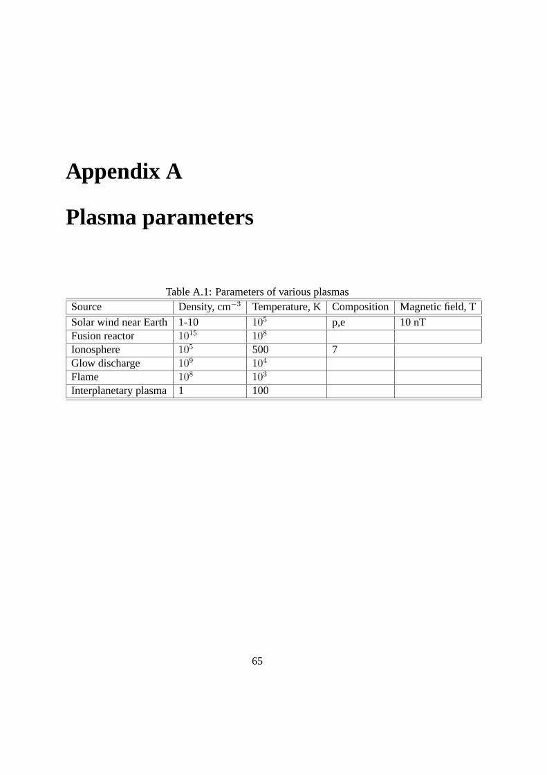
Appendix A

Plasma parameters

Table A.1: Parameters of various plasmasSource Density, cm−3 Temperature, K Composition Magnetic field, T

Solar wind near Earth 1-10 105 p,e 10 nTFusion reactor 1015 108

Ionosphere 105 500 7Glow discharge 109 104

Flame 108 103

Interplanetary plasma 1 100

65

Date post:	13-Feb-2018
Category:	Documents
Upload:	truongque
View:	216 times
Download:	1 times

Michael Gedalin - Purdue Department of Physics and ...lyutikov/phys670/Gedalinplasma.pdf ·...

Documents