267
| Date post: | 27-Nov-2015 |
| Category: |
Documents |
| Upload: | cristina-boboaca |
| View: | 29 times |
| Download: | 0 times |

Exchange Rate Regimes in the Modern Era


Exchange Rate Regimes in the Modern Era
Michael W. Klein and Jay C. Shambaugh
The MIT Press
Cambridge, Massachusetts
London, England

( 2010 Massachusetts Institute of Technology
All rights reserved. No part of this book may be reproduced in any form by any elec-tronic or mechanical means (including photocopying, recording, or information storageand retrieval) without permission in writing from the publisher.
For information about special discounts, please email [email protected]
This book was set in Palatino on 3B2 by Asco Typesetters, Hong Kong.Printed and bound in the United States of America.
Library of Congress Cataloging-in-Publication Data
Klein, Michael W., 1958–.Exchange rate regimes in the modern era / Michael W. Klein and Jay C. Shambaugh.p. cm.
Includes bibliographical references and index.ISBN 978-0-262-01365-9 (hbk. : alk. paper)1. Foreign exchange rates. 2. Foreign exchange. I. Shambaugh, Jay C. II. Title.HG3851.K57 2010332.405—dc22 2009014104
10 9 8 7 6 5 4 3 2 1

To Susan, Gabe, and Noah
MWK
To Lisa, Katie, and Jack
JCS


Contents
Acknowledgments ix
I Introduction 1
1 Exchange Rate Regimes in the Modern Era 3
II The Nature of Exchange Rate Regimes 11
2 Exchange Rate Regimes in Theory and Practice 13
3 Exchange Rate Regime Classifications 29
4 The Dynamics of Exchange Rate Regimes 51
5 The Empirics of Exchange Rate Regime Choice 73
III Exchange Rate Consequences of Exchange Rate Regimes 99
6 Exchange Rate Regimes and Bilateral Exchange Rates 101
7 Exchange Rate Regimes and Multilateral Exchange Rates 117
IV Economic Consequences of Exchange Rate Regimes 131
8 Exchange Rate Regimes and Monetary Autonomy 133
9 Exchange Rate Regimes and International Trade 147
10 Exchange Rate Regimes and Inflation 165
11 Exchange Rate Regimes and Economic Growth 185

V Conclusion 203
12 Exchange Rate Regimes in an Interdependent World 205
Notes 209
References 229
Index 241
viii Contents

Acknowledgments
This book represents over a decade of work in thinking, researching,
and writing about exchange rate regimes. Along the way, in both pro-
ducing this book during the last year, and in generating the research
that has gone into it over the last decade, many people have helped
us. It is a pleasure to acknowledge them, and to thank them for their
support.
First and foremost, we would like to thank our fellow scholars,
many of whom had a hand in generating the research discussed in this
book. Various chapters draw on joint work with Julian di Giovanni,
Philip Lane, Nancy Marion, Maurice Obstfeld, and Alan Taylor. We
thank them for working with us, and, more broadly, for contributing
to our understanding and appreciation of these issues. In addition, the
work in this book was presented at numerous seminars and confer-
ences, and we owe a great deal to seminar participants and discus-
sants, as well as to others who offered comments on our research
papers and drafts of this book, including Sven Arndt, Christian Broda,
Menzie Chinn, Barry Eichengreen, Charles Engel, Jeff Frankel, Allen
Isaac, Richard Levich, Paolo Mauro, Volker Nitsch, Andy Rose, Lars
Svensson, Linda Tesar, Eric van Wincoop, and John Williamson. Other
colleagues and friends also gave advice regarding both presentation
and empirical strategies, and we thank Steven Block, Eric Edmonds,
James Feyrer, Jeff Frieden, Linda Goldberg, Matt Kahn, Doug Irwin,
Chris Meissner, Nina Pavcnik, and Doug Staiger. Of course, in thank-
ing all these people we do not mean to implicate them for any short-
comings in this book.
Jane Macdonald at the MIT Press has been a wonderful guide
through the process of getting this book to publication, and we thank
her, the marketing staff, and production team for their efforts. In addi-
tion five anonymous reviewers gave us very useful feedback on an
initial draft of the book.

We thank our teachers at various stages of our own academic careers
for their guidance and support in helping us explore our intellectual
interests, and for teaching us how to develop our ideas and share
them with the world. In particular, we would like to thank Maury
Obstfeld. Maury was the dissertation advisor to each of us, albeit at
two different times and on two different coasts of the United States.
We both greatly value his mentoring and friendship over the years.
Most of all, we thank our families for their encouragement, support,
and patience as we crafted this manuscript. Parents, siblings, spouses,
and children have all played essential roles in helping us reach the
point where we could write this book, and in providing the time and
encouragement for us to complete it.
MWK and JCS
x Acknowledgments

If art from the third quarter of the nineteenth century to the last quarter of the twen-tieth century is an ‘‘era,’’ corresponding in some way to the era inaugurated by theRenaissance, then this modern era is one that contains a confusing multiplicity ofvisual styles.
—David Britt, Modern Art: From Impressionism to Post-Modernism, c. 1974


I Introduction


1 Exchange Rate Regimes in the Modern Era
The dollar’s exchange rate against the euro is surely the world’s single mostimportant price, with potentially much bigger economic consequences thanthe price of oil and computer chips, for example.
—‘‘The not so mighty dollar,’’ The Economist, December 4, 2003
The dollar–euro exchange rate, perhaps ‘‘the world’s single most im-
portant price,’’ is determined by market forces, and changes day to
day, and even minute to minute. In contrast, each of the countries of
the European Union that uses the euro as its national currency experi-
ences no exchange rate changes with the other members of the euro-
zone because they share a common currency. Why is it that the United
States allows its currency to float, while Germany, France, and the
other members of the eurozone have abandoned their national curren-
cies and, effectively, have set a fixed exchange rate across Europe? Sim-
ilarly, why does the government of China fix the value of its yuan to
the US dollar, while the world foreign exchange market determines
the daily value of the Brazilian real? The overarching policy of the gov-
ernment toward the exchange rate—to allow it to float or instead to fix
or peg its value to another currency—is called the exchange rate re-
gime. What are the economic and political implications of these differ-
ent exchange rate regimes for these nations?
Questions of this type are quite important today, in this modern era
of exchange rate regimes. The modern era includes a wide variety of
exchange rate regime experiences across countries. Furthermore, dur-
ing the modern era, many countries have switched from one type of
exchange rate regime to another and often have flipped back and forth
another time or two.
The widespread ability of governments to choose an exchange rate
regime distinguishes the modern era from earlier periods.1 Before 1973

the choice of whether or not to manage the value of a currency was
often bound up with the wider choice of participation in the interna-
tional monetary and trading system. During the classical gold standard
period (1880–1914) it was generally the case that access to the world
capital market demanded pegging the value of a country’s currency to
gold, since this peg served as a country’s ‘‘Good Housekeeping Seal of
Approval.’’2 There was also a view that participation in the gold stan-
dard benefited countries by promoting their trade with other countries
that pegged their currency to gold. Some countries only slowly
adopted a gold peg and a handful of countries changed their regime,
but by and large, countries participating in the world financial and
trade system moved toward a gold peg.3 Decades later, during the
Bretton Woods era (1945–1973), the adoption of a fixed exchange rate
to the US dollar was one facet of participation in the international mon-
etary system, with other facets including membership in the Bretton
Woods institutions—the International Monetary Fund and the Interna-
tional Bank for Reconstruction and Development (the World Bank)—
and in the General Agreement on Trade and Tariffs (the GATT). In
both of these eras, pegged exchange rates were pervasive across coun-
tries and durable among the countries that pegged.
The modern era has lasted longer than both the Bretton Woods and
the classic gold standard periods. It differs from these two earlier peri-
ods in important ways. Most notably, the modern era is distinguished
by its wide variety of exchange rate experiences for industrial, middle
income, emerging market, and developing countries.4 This period has
seen everything from the abandonment of a national currency (e.g.,
Ecuador’s use of the US dollar, and the creation of the euro), experi-
ence with a currency board (e.g., Hong Kong, Lithuania, and Argen-
tina), fixed exchange rates (e.g., Saudi Arabia, Mexico, and South
Korea), exchange rate bands (the European Monetary System which
lasted from 1979 to 1999), heavily managed floating exchange rates
(Norway), occasional efforts to stem the appreciation (1985) or slide
(1995) of the US dollar, and the benign neglect of a floating exchange
rate (United States, 1979–1985).
The exchange rate regime experiences of the modern era provide
researchers with a colorful palette, one with enough hues to make it
possible to address interesting and important questions about the na-
ture and consequences of exchange rate regime choice. In this book we
will both characterize the choice of exchange rate regimes in the mod-
ern era and present empirical research that demonstrates the effects of
4 Chapter 1

this choice on macroeconomic outcomes and international trade. We
address some of the long-standing central issues in international
finance, including the pattern of exchange rate regime behavior, the
interaction between the exchange rate regime and monetary policies
(which is known as the policy trilemma), the influence of exchange
rate regimes on the volume and pattern of international trade, and the
links between exchange rate regimes and general macroeconomic out-
comes such as GDP growth and inflation.
One source of inquiry into the implications of exchange rate regime
choice was prompted by the fact that exchange rate volatility at the be-
ginning of the modern era was higher than what economists had gen-
erally expected. There had not been much actual experience with
floating exchange rates among major industrial countries during the
Bretton Woods era, save for the Canadian dollar’s float in the 1950s.
Floating currencies in the modern era are not simply episodes where
countries are unable to peg but generally represent a deliberate choice
to float. At the start of the modern era, the prevailing theory had sug-
gested that floating exchange rates might not be especially volatile.
The monetary approach to exchange rate suggested that the volatility
of the bilateral exchange rate linking two currencies would match the
volatility of the difference of the two countries’ respective money sup-
plies and outputs.5 Milton Friedman (1953) had already argued force-
fully that speculators would stabilize exchange rates. As it turned out,
however, exchange rates were much more volatile than fundamentals
at a short horizon, and, even at longer horizons, exchange rates of in-
dustrial countries seemed to persistently deviate from fundamental
values. Partly for these reasons the exchange rate overshooting model
of Dornbusch (1976), which showed how exchange rate volatility
results from slowly adjusting goods’ prices, captured the attention of
the economics profession and became the most cited paper in interna-
tional economics.6 Analyses of the implications of the choice of a flexi-
ble exchange rate regime in the modern era that are presented in this
book will reflect the volatility of floating exchange rates.
Experiences with fixed exchange rates during the modern era also
led to new analyses. Countries peg to different base currencies for
varying periods of time. Many of their key economic partners may not
peg, may peg to a different base, or may break the peg at different
intervals. The motivations to peg (controlling inflation, stimulating
trade, avoiding volatility) have varied as have the reasons for leaving
pegs. Overall, however, there have been a large number of spectacular
Exchange Rate Regimes in the Modern Era 5
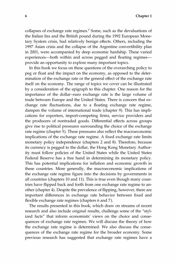
collapses of exchange rate regimes.7 Some, such as the devaluations of
the Italian lira and the British pound during the 1992 European Mone-
tary System crisis, had relatively benign effects. Others, including the
1997 Asian crisis and the collapse of the Argentine convertibility plan
in 2001, were accompanied by deep economic hardship. These varied
experiences—both within and across pegged and floating regimes—
provide an opportunity to explore many important topics.
In this book we focus on these questions of the overarching policy to
peg or float and the impact on the economy, as opposed to the deter-
mination of the exchange rate or the general effect of the exchange rate
itself on the economy. The range of topics we cover can be illustrated
by a consideration of the epigraph to this chapter. One reason for the
importance of the dollar–euro exchange rate is the large volume of
trade between Europe and the United States. There is concern that ex-
change rate fluctuations, due to a floating exchange rate regime,
dampen the volume of international trade (chapter 9). This has impli-
cations for exporters, import-competing firms, service providers and
the producers of nontraded goods. Differential effects across groups
give rise to political pressures surrounding the choice of the exchange
rate regime (chapter 5). These pressures also reflect the macroeconomic
implications of the exchange rate regime. A fixed exchange rate limits
monetary policy independence (chapters 2 and 8). Therefore, because
its currency is pegged to the dollar, the Hong Kong Monetary Author-
ity must follow policies of the United States while the United States
Federal Reserve has a free hand in determining its monetary policy.
This has potential implications for inflation and economic growth in
these countries. More generally, the macroeconomic implications of
the exchange rate regime figure into the decisions by governments in
all countries (chapters 10 and 11). This is true even though many coun-
tries have flipped back and forth from one exchange rate regime to an-
other (chapter 4). Despite the prevalence of flipping, however, there are
important differences in exchange rate behavior between fixed and
flexible exchange rate regimes (chapters 6 and 7).
The results presented in this book, which draw on streams of recent
research and also include original results, challenge some of the ‘‘styl-
ized facts’’ that inform economists’ views on the choice and conse-
quences of exchange rate regimes. We will discuss the theory of how
the exchange rate regime is determined. We also discuss the conse-
quences of the exchange rate regime for the broader economy. Some
previous research has suggested that exchange rate regimes have a
6 Chapter 1
limited impact on general economic outcomes. We will provide empir-
ical results, however, showing the exchange rate regime often plays an
important role in the economy.
In part II we discuss the nature of exchange rate regimes themselves.
Chapter 2 reviews overarching frameworks on both the choice and
effects of exchange rate regimes. The next chapter of that section fo-
cuses on what we mean by the term ‘‘exchange rate regime.’’ The dis-
cussion in chapter 3 raises issues that arise when considering the
classification of exchange rate regimes, and presents four different clas-
sification schemes that have been used by researchers. In chapter 4 we
present characteristics of exchange rate regimes in the modern era that
challenge some of the standard views presented in chapter 2 by show-
ing that the pattern of exchange rate regimes during the past four de-
cades is marked by pervasive ‘‘flipping,’’ that is, going off a peg for a
short period of time and then reestablishing a new peg. Of course, this
means that the short duration of pegged exchange rates is matched by
a short duration of periods during which a country has a floating ex-
change rate. This is an important result because it calls into question
any study that dichotomizes the world into a set of countries that have
durable pegs and a set of countries that consistently have market-
determined flexible exchange rates. We also show, however, that there
are important examples of long-lived fixed exchange rate regimes in
the modern era, contrary to the impression one would draw from
some influential research published in the 1990s that calls fixed ex-
change rates a ‘‘mirage.’’8 Part II concludes with a chapter that ana-
lyzes the manner in which countries choose an exchange rate regime.
There are both political and economic theories on this topic. Empirical
results presented in chapter 5 offer support for both sets of theories in
explaining countries tendencies toward one type of exchange rate re-
gime or another.
The dichotomy between fixed and floating exchange rates is mean-
ingful only if there is evidence that behavior under these two exchange
rate regimes differs significantly. Part III of this book shows that the
behavior of nominal and real exchange rates in fact depends on the
exchange rate regime in place. At one level, this would seem to be a
tautological point; if we define a fixed exchange rate as one that does
not change by a certain amount over a specified period, then it must
differ from a flexible exchange rate. There are two reasons to examine
this issue more closely, however. The first is that the recent ‘‘fear
of floating’’ result claims little actual difference in nominal bilateral
Exchange Rate Regimes in the Modern Era 7
floating exchange rates from nominal bilateral fixed rates.9 We exam-
ine this claim in chapter 6, and show that there is a significant and eco-
nomically meaningful difference between fixed and floating exchange
rates. Second, an exchange rate is only pegged against one other cur-
rency. A peg against a base currency does not ensure stability against
other currencies, some of which may be especially important for multi-
lateral trade or investment. We study the multilateral consequences of
bilateral pegging in chapter 7.
In part IV we turn from characterizing exchange rate regimes to con-
sidering their consequences. One of the central theoretical results in in-
ternational finance is the policy trilemma, whereby the government of
a country can choose a pair from the triplet of exchange rate manage-
ment, monetary policy autonomy, and international capital mobility.
While this is a well-established theoretical result, its empirical validity
has recently been called into question. We examine this central debate
in empirical international finance in chapter 8, and conclude that the
policy trilemma is alive and well.
Another important economic impact of exchange rate regimes is the
effect on international trade. Studies dating from the 1970s based on
the estimation of import and export equations have failed to find
much evidence that a fixed exchange rate regime promotes bilateral
trade. More recently, however, an alternative methodology using esti-
mates of gravity equations for trade has presented compelling evi-
dence for the statistically significant and economically meaningful
effects of fixed exchange rates on trade. We discuss the evolution of
this literature, and present results showing the effect of the exchange
rate regime on trade in chapter 9.
Fixing the exchange rate may provide a nominal anchor for the econ-
omy by fixing the price of one particular asset to help discipline the
central bank from printing too much money. This should reduce infla-
tion. In addition a persistently pegged exchange rate should temper
the expectation of inflation, which itself dampens inflation. There is a
long-standing literature suggesting that this could work in theory. We
review this theory in chapter 10, and also offer new evidence that
shows a role for the exchange rate regime in the determination of
inflation.
Ultimately, the central concern in economics is living standards.
Thus we conclude in part IV with an examination of whether exchange
rate regimes affect growth of real GDP. A number of studies lately
(Levy-Yeyati and Sturzenegger 2003; Rogoff et al. 2006; etc.) have con-
8 Chapter 1

sidered the question but with different classifications, different sam-
ples, and different econometric techniques, and consequently, different
results. We use common data and techniques to compare results across
classifications. We find that the impact of the exchange rate regime on
long run GDP growth, controlling for other factors, is relatively weak.
This stands in contrast to some influential results in the literature.
In the 2000s answers to questions about the effects of exchange rate
regimes on economic performance, and the very nature of exchange
rate regimes, have changed with new empirical analyses. Previous
skepticism regarding the importance of the exchange rate regime for
economic outcomes has been challenged. It is the nature of research
that the answers to questions change, even questions that are at the
core of a subject. The topics discussed in this book represent classic
questions in international finance. Views on these topics have changed
as the modern era has progressed, and as new experiences are incorpo-
rated into studies. We show in this book that the exchange rate regime
can have significant impacts on a variety of aspects of the economy.
Our goal is to contribute to our understanding of the modern era and,
in so doing, to deepen our knowledge of some of the central empirical
issues in international finance.
Exchange Rate Regimes in the Modern Era 9

II The Nature of Exchange Rate Regimes


2 Exchange Rate Regimes in Theory and Practice
So much of barbarism, however, still remains in the transactions of most civi-lized nations that almost all independent countries choose to assert their na-tionality by having, to their own inconvenience and that of their neighbors, apeculiar currency of their own.
—John Stuart Mill, Principles of Political Economy, 1848
A system of flexible or floating exchange rates [is] . . . absolutely essential for thefulfillment of our basic economic objective: the achievement and maintenanceof a free and prosperous world community engaged in unrestricted multilat-eral trade.
—Milton Friedman, ‘‘The case for flexible exchange rates,’’ 1953
More than a full century separates John Stuart Mill’s writing of the
‘‘barbarism’’ of countries desiring their own currencies, and Milton
Friedman’s argument that flexible exchange rates are ‘‘absolutely es-
sential’’ for economic prosperity. If economics progressed like the
natural sciences, one might be able to say that Friedman’s mid-
twentieth-century perspective favoring flexible exchange rates reflected
an advance in knowledge over Mill’s mid-nineteenth-century view of
the desirability of fixed exchange rates backed by precious metals, just
as physicists’ understanding of electromagnetism today is more subtle
than that developed by Michael Faraday, Mill’s contemporary. One
could even hope that today, at the beginning of the twenty-first cen-
tury, we might have arrived at a resolution on this central issue of in-
ternational macroeconomics. But this is not the case. The debate over
the relative benefits and costs of different exchange rate regimes re-
mains lively.
Of course, there have been advances in our understanding of the
implications of exchange rate regimes in the century-and-a-half since

the time of Mill, and in the decades since Friedman wrote his classic ar-
ticle. But some of the issues raised by these great economists remain
relevant today.1 Mill was concerned with instability affecting trade
and commerce when national currencies were not anchored to pre-
cious metals. These concerns are mirrored in contemporary efforts by
central banks to gain credibility by pegging exchange rates to the cur-
rencies of countries with a history of relatively low inflation. Friedman,
on the other hand, thought that flexible exchange rates could facilitate
market adjustment. Debate over the appropriate exchange rate policies
of countries like China that run large and persistent trade imbalances
while pegging their currencies echo the arguments raised by Friedman
more than a half-century ago.
In this chapter we provide a context for much of the rest of the book
by introducing standard views on exchange rate regimes and their eco-
nomic consequences. Exchange rate regimes can be analyzed using
various frameworks, and arguments based on these different perspec-
tives motivate much of the empirical work throughout the rest of this
book. Section 2.1 considers the constraints imposed on macroeconomic
policy by fixed exchange rates, a topic that is the focus of chapter 9.
Section 2.2 examines the arguments for fixing the exchange rate in
order to stabilize the economy, a topic explored in chapter 11. Section
2.3 presents a theory that offers guidance for whether countries or
regions should use a common currency that is based on the balance be-
tween macroeconomic flexibility and economic integration, a topic dis-
cussed in chapters 10 and 12. Section 2.4 surveys the political economy
motives for exchange rate regime choice that, as discussed further in
chapter 5, may dominate purely economic considerations when gov-
ernments make the decision of whether to peg their currency. We
draw on these frameworks as we conclude this chapter with a discus-
sion of exchange rate regimes and the international monetary system
over the last 150 years. This brief history provides a context for our
analysis of the modern era.
The standard textbook exposition of exchange rate regimes places
countries into one of two categories: those that fix the price of their cur-
rency against that of another currency (or, synonymously, peg their
currency), and those that allow their currency to float and be deter-
mined by market forces. This categorization is pedagogically conve-
nient, and in this section we will use it to discuss some standard
results from international macroeconomics. But we also note up front
that as shown in the next two chapters, there are few examples of
14 Chapter 2
countries that have persistently maintained either of these two polar
stances over the entire modern era. Further there are differences be-
tween a currency peg and abandoning a national currency altogether
via dollarization (e.g., as in Ecuador) or a currency union (e.g., as in
the euro area).2 Frequently the issues involved in the decision to peg
or float are similar to those arising when considering the formation of
a currency union, but we will note where the distinction is important.
Also, as discussed in the chapter 3, there are a range of intermediate
regimes between these extremes of a free float and a stable peg. Never-
theless, there are valuable insights one gains from considering the dif-
ferences between the textbook versions of fixed and flexible exchange
rate regimes even though a complete understanding of exchange rate
regimes in the modern era requires us to go well beyond this simple
dichotomy.
2.1 The Open Economy Trilemma
The clean division of countries into those that fix and those that float
allows for the straightforward illustration of a central result in interna-
tional macroeconomics, the policy trilemma.3 The policy trilemma
states that the monetary authorities of a country can choose no more
than two of three policy options: free capital mobility, fixed exchange
rates, and domestic monetary autonomy. This then limits the scope for
a country’s policy options.
The policy trilemma is sometimes depicted using the diagram in fig-
ure 2.1. The corners of this triangle represent three policy options fac-
ing a government: free capital mobility, which allows people in a
country to transfer funds abroad and people outside a country to pur-
chase its assets; a fixed exchange rate (or peg), which enables a govern-
ment to fix the bilateral exchange rate with another country; and
monetary autonomy, which means that a country’s central bank has a
free hand in setting monetary policy. The sides of the triangle represent
the policy options available to a government. For example, side A in
this figure represents the choice of an exchange rate peg and free capi-
tal mobility, implying the country has forgone domestic monetary au-
tonomy while side B represents the choice of monetary autonomy and
free capital mobility meaning the country does not attempt to manage
its exchange rate. The key point of the policy trilemma is that a govern-
ment can choose a pair of policies corresponding to A, B, or C, but does
not have the ability to simultaneously fix the exchange rate, control the
Exchange Rate Regimes in Theory and Practice 15

money supply, and allow for free capital mobility. The theory does not
require that a government choose a pure corner solution, embracing
two policies and abandoning the other altogether. Rather, there are
trade-offs across the three policies. For example, there is an increas-
ingly large sacrifice of monetary autonomy or capital mobility (or
both) as a government attempts to have greater control of its exchange
rate.
The reason that governments are constrained in a way described by
the policy trilemma can be understood using any one of a number of
macroeconomic models of an open economy. The fundamental aggre-
gate relationships in these models do not depend on the exchange rate
regime in place. Rather, in these models, the choice of exchange rate re-
gime determines which variables are exogenous and determined by
authorities, and which are endogenous and the outcome of markets.
Under flexible exchange rates the monetary authorities choose an inter-
est rate that suits domestic economic considerations. In this case the
value of the exchange rate reflects this choice as well as the value of
other exogenous factors, like domestic fiscal policy, exogenous domes-
tic investment demand, or the foreign interest rate. The exchange rate
will also depend on expectations of its future value. In contrast, a fixed
exchange rate regime requires that monetary policy is directed toward
the maintenance of the pegged value of the exchange rate. In this case,
monetary policy meets this goal by responding passively to peg the
value of the currency in the face of changing economic circumstances,
or changing perceptions about the future.4
Figure 2.1
The policy trilemma.
16 Chapter 2
If capital markets are open and the exchange rate is fixed (and is
expected to stay pegged at a constant rate), the interest rate on a repre-
sentative domestic bond must equal the interest rate on a similar bond
denominated in the currency of the country to which the exchange rate
is pegged. If the interest rate on the domestic bond was lower, inves-
tors would clearly favor the foreign bond, and, consequently, domestic
investors would purchase foreign exchange in order to buy the higher
yielding foreign bond. This would force the domestic central bank to
sell its foreign currency in order to short-circuit an excess demand for
foreign currency that would cause the domestic currency to weaken
and would break the peg if the central bank did not respond. The
resulting decrease in the domestic money supply would raise the inter-
est rate on the domestic bond to parity with that of the foreign bond
(this illustrates the lack of monetary autonomy with a fixed exchange
rate and open capital markets). If, however, the central bank attempted
to maintain some monetary autonomy and forestall this interest rate
increase, it would eventually run out of foreign exchange; at that point
the peg would break and there would be a devaluation of the domestic
currency. In this case the trilemma operates through giving up ex-
change rate management in order to have monetary autonomy.
The policy trilemma thus shows that with capital mobility, monetary
policy becomes subordinated to pegging the value of the currency for a
country operating with a fixed exchange rate, or for countries in a cur-
rency union. A country that pegs its currency to that of another coun-
try must follow the monetary policy of that country. Also there is only
a single monetary policy for all countries participating in a currency
union. There are important implications of this for understanding the
relative merits of fixed versus flexible exchange rates. One source of
concern with fixed exchange rates in the presence of capital mobility is
that governments that peg their currencies lose the use of a potentially
important stabilization policy. The cost of foregoing monetary auton-
omy for a particular country depends on the extent to which the mone-
tary policy of the base country mimics the monetary policy that it
would undertake were it to have the latitude to set this policy inde-
pendently.5 We explore the empirical relevance of the policy trilemma
in chapter 8.
2.2 Fixed Exchange Rates and Stabilization Policy and Adjustment
The loss of monetary policy autonomy may, in certain circumstances,
even benefit a country. One example is when the automatic monetary
Exchange Rate Regimes in Theory and Practice 17

policy response that occurs with a fixed exchange rate serves to stabi-
lize an economy. Such could be the case for a small economy that is
open to trade and depends on a particular export for much of its for-
eign exchange revenues. The small economy’s exchange rate whose
value is pegged to the price of the main export commodity would then
depreciate with a fall in that price, helping to offset contractionary
effects, and appreciate with a rise in that price, mitigating the expan-
sion due to the favorable change in the country’s terms of trade.6
Another example of the advantageous automatic stabilization prop-
erties of a fixed exchange rate, in this case for a more diversified econ-
omy than the one considered in the previous paragraph, occurs when
potential disruptions come from asset markets or unstable money de-
mand, rather than goods markets. In this case the appropriate policy
response would be to offset these shocks through monetary policy. In
contrast, when the economy is buffeted by events like a collapse in in-
vestment demand, or an increase in the price of oil or food, policies to
maintain a fixed exchange rate could exacerbate problems. In these
cases a flexible exchange rate system may be more desirable, since the
exchange rate serves as a shock absorber for the economy.7 Its depreci-
ation in the face of adverse shocks of this type, and its appreciation
when the economy is stimulated due to an expansion in the demand
for goods, mitigates the overall movement in national income. In con-
trast, a fixed exchange rate exacerbates the effects of these shocks on
national income. In essence, recognition of this type of stabilization
from flexible exchange rates led to the acceptance of widespread float-
ing at the beginning of the modern era while countries were trying to
adapt to rapid increases in the price of oil and food.8
Another situation where there is an advantage to surrendering mon-
etary policy autonomy to the requirements of a fixed exchange rate
occurs when a central bank fails to perform well if left to its own dis-
cretion. This is one basis of Mill’s argument for fixing the exchange
rate to the value of a precious metal. More recently economists have fo-
cused on the consequences of the perception of central bank profligacy,
and how to anchor people’s expectations to improve economic perfor-
mance. Research on central bank credibility shows that rules that bind
the actions of a central bank can result in a better outcome than what
would occur without this type of commitment.9 As shown by the pol-
icy trilemma, a fixed exchange rate can serve as this type of rule since,
with open capital markets, a central bank that must maintain a peg
does not have a free hand to set monetary policy. In fact, because the
18 Chapter 2
efficacy of a rule depends, in part, on the ability of people to under-
stand the rule and to be able to verify adherence to it, a fixed exchange
rate may be a particularly useful commitment device for a monetary
authority. The exchange rate is a very public price and is known in the
market at all times; thus, actors in the economy are constantly aware of
whether the central bank is maintaining its commitment. For this rea-
son, a number of countries have centered stabilization plans on an ex-
change rate goal, including Argentina, Chile, Uruguay, and Israel.10
Furthermore European countries that had a history of poor inflation
performance, like Italy, saw a monetary union as a way to import anti-
inflation credibility and, in so doing, more easily bring down inflation
in their own country. Chapter 10 presents an empirical analysis of the
effect of fixed exchange rates on inflation.
These efforts to stabilize economies through a fixed exchange rate
have often not worked out well, however. Most exchange-rate-based
stabilization plans have not succeeded in a sustained reduction in infla-
tion (Vegh 1992). Also the history of the last four decades is littered
with examples of spectacular collapses of fixed exchange rate regimes.
These include several episodes in Latin America (including Mexico in
1982 and 1994, and Argentina in 2001–2002), the collapse of the Euro-
pean Monetary System in 1992, and the 1997–1998 Asian crises. In
some of these cases, like Argentina in 2002 and Thailand in 1997, these
initial exchange rate collapses were followed by severe economic hard-
ship. In other cases, like the United Kingdom in 1992, the exchange
rate devaluation spurred exports and led to economic growth.
Fixed exchange rates can also lead to problems when they help sus-
tain differences in relative prices across countries that lead to trade
imbalances and painful adjustment through rising unemployment in
countries with trade deficits, and unwanted inflationary pressures in
countries with trade surpluses.11 In particular, it is often easier to have
a currency depreciation in the face of a trade deficit than to rely on
overall price deflation. As mentioned above, Milton Friedman argued
in 1950 that flexible exchange rates could facilitate this process, writ-
ing, ‘‘It is far simpler to allow one price to change, namely, the price of
foreign exchange, than to rely upon changes in the multitude of prices
that together constitute the internal price structure’’ (ibid., p. 173).
This view, that flexible exchange rates would smoothly allow for
overall trade adjustment, was common then. For example, Sidney
Wells begins the chapter entitled ‘‘For and Against Fluctuating Ex-
change Rates’’ in his 1968 textbook International Economics:
Exchange Rate Regimes in Theory and Practice 19

The first and most obvious advantage of a fluctuating exchange rate is . . . de-preciation or appreciation can be expected automatically to restore equilibriumin a country’s balance of payments. There is no need for unemployment to becreated or restrictions to be imposed in order to reduce imports and increaseexports. (p. 192)
But experiences have shown that flexible exchange rates have not
served to maintain balanced trade, nor have they kept countries from
suffering unemployment due to competition from other countries. An
important reason for this is that exchange rates respond strongly to
asset market conditions, and not just trade imbalances. Real exchange
rates, that is, exchange rates adjusted for price differentials across
countries, move around for reasons unrelated to trade while having a
strong impact on exports, imports, and economic activity related to
these activities.12
2.3 Optimum Currency Areas
The previous section has shown that neither theory nor experience pro-
vides support for unambiguously favoring one exchange rate regime
over another. While economics often looks for a single optimal solution
to a problem, the simple truth is that the appropriate exchange rate
regime depends on the particular circumstances of a country.13 An
influential line of research does, however, provide some guidance
concerning which exchange rate regime might be appropriate for a
particular country. This research began with the 1961 contribution of
Robert Mundell, research that was cited when he was awarded the
Nobel Memorial Prize in Economics in 1999. In this paper Mundell
offers criteria for an optimum currency area (OCA).14
As Mill argues, national currencies are inconvenient because they
make international exchange of goods and services more difficult by
forcing people to trade currencies when they purchase something from
another country (or, depending on the way the exchange is structured,
when they sell something to another country). While this is true with
fixed as well as flexible exchange rates, credibly fixed exchange rates
have the virtue of locking in the domestic currency price of a future
payment denominated in foreign currency. This could theoretically
promote international trade by reducing uncertainty, and as shown in
chapter 9, there is empirical support for this argument since trade is
higher, all else held equal, between two countries with a fixed ex-
change rate than between two countries with a flexible exchange rate.
20 Chapter 2
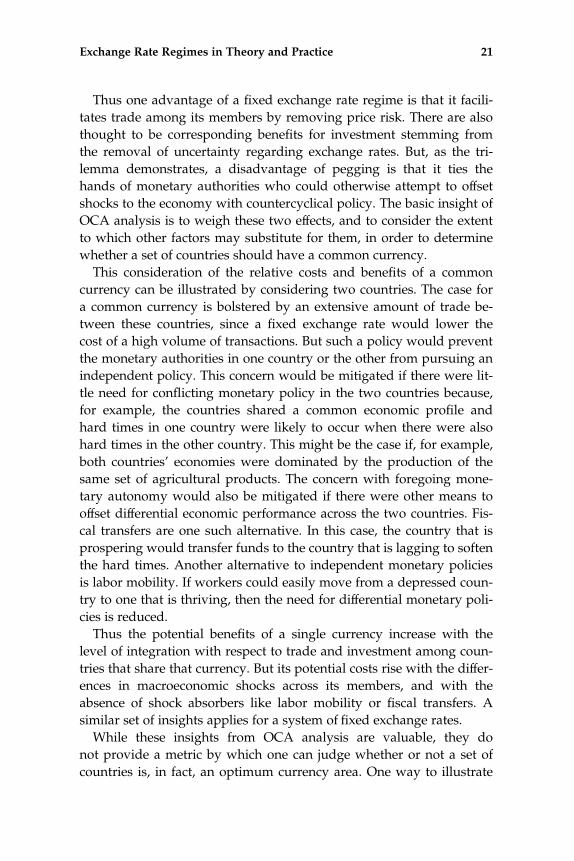
Thus one advantage of a fixed exchange rate regime is that it facili-
tates trade among its members by removing price risk. There are also
thought to be corresponding benefits for investment stemming from
the removal of uncertainty regarding exchange rates. But, as the tri-
lemma demonstrates, a disadvantage of pegging is that it ties the
hands of monetary authorities who could otherwise attempt to offset
shocks to the economy with countercyclical policy. The basic insight of
OCA analysis is to weigh these two effects, and to consider the extent
to which other factors may substitute for them, in order to determine
whether a set of countries should have a common currency.
This consideration of the relative costs and benefits of a common
currency can be illustrated by considering two countries. The case for
a common currency is bolstered by an extensive amount of trade be-
tween these countries, since a fixed exchange rate would lower the
cost of a high volume of transactions. But such a policy would prevent
the monetary authorities in one country or the other from pursuing an
independent policy. This concern would be mitigated if there were lit-
tle need for conflicting monetary policy in the two countries because,
for example, the countries shared a common economic profile and
hard times in one country were likely to occur when there were also
hard times in the other country. This might be the case if, for example,
both countries’ economies were dominated by the production of the
same set of agricultural products. The concern with foregoing mone-
tary autonomy would also be mitigated if there were other means to
offset differential economic performance across the two countries. Fis-
cal transfers are one such alternative. In this case, the country that is
prospering would transfer funds to the country that is lagging to soften
the hard times. Another alternative to independent monetary policies
is labor mobility. If workers could easily move from a depressed coun-
try to one that is thriving, then the need for differential monetary poli-
cies is reduced.
Thus the potential benefits of a single currency increase with the
level of integration with respect to trade and investment among coun-
tries that share that currency. But its potential costs rise with the differ-
ences in macroeconomic shocks across its members, and with the
absence of shock absorbers like labor mobility or fiscal transfers. A
similar set of insights applies for a system of fixed exchange rates.
While these insights from OCA analysis are valuable, they do
not provide a metric by which one can judge whether or not a set of
countries is, in fact, an optimum currency area. One way to illustrate
Exchange Rate Regimes in Theory and Practice 21

these concepts, however, is to consider a benchmark case. In recent
years, especially in the period leading up to the single currency in Eu-
rope, the benchmark used by many researchers is the United States.
The United States is a very large and economically diverse country.
One could imagine a situation in which regions of the United States
had independent currencies; there could be a New England dollar, a
mid-Atlantic dollar, a southern dollar, and so on. This would, of
course, complicate trade across regions. The cost of trade would rise,
and given the extensive amount of trade that occurs between New
York and Texas, or California and Illinois, this would represent a large
cost to the United States.
But what about the benefits of regional currencies? Separate curren-
cies that floated against each other would allow regional monetary
authorities to respond to local needs. There have been large disparities
in economic performance across regions in recent years, such as the
waning fortunes of the Midwest in the 1980s when the term ‘‘rustbelt’’
was coined, the downturn in New England in the early 1990s in the
wake of changes in the hi-tech sector, and the way in which the for-
tunes of Texas change with the price of oil. Wouldn’t it be advanta-
geous to have policy responses to these local disruptions, even given
the increased cost of trade arising from regional currencies?
The generally agreed-upon answer to this question is ‘‘no.’’ While
acknowledging ongoing regional differences in economic performance,
economists also point to mechanisms that serve as a substitute for re-
gional monetary policies. National fiscal policy serves as an automatic
stabilizer across regions. A region in recession will pay less federal tax
and receive more transfers from Washington. Labor mobility is also an
important feature of the United States economy. Workers leave areas
that are suffering an economic downturn, moving to more prosperous
areas, and this helps mitigate the effects of regional recessions. Overall,
then, no one argues that the United States should give up the national
currency for regional monies.15
There was, of course, a protracted argument on whether European
countries should abandon their national currencies for the euro in the
1990s. Economists considered the question of the desirability of a sin-
gle currency in light of OCA arguments, and some used the United
States as a benchmark.16 In these comparisons Europe did not seem
nearly as desirable a currency area as the United States because of the
lower amount of intra-European trade as compared to trade within the
United States, the paucity of transfers from a central European author-
22 Chapter 2

ity to separate countries as compared to federal transfers in the United
States, and the much lower level of labor mobility across European
countries (or, as it turns out, even within European countries) as com-
pared to the footloose nature of Americans. But perhaps this was too
high a bar. While the United States is inconvertibly an OCA, maybe
Europe is as well, even though its case is not as strong.
As discussed in chapter 5, there is empirical support for the view
that a country’s choice of an exchange rate regime is based on eco-
nomic considerations raised by OCA theory. But, as shown in that
chapter, there is also evidence that other, noneconomic arguments sig-
nificantly contribute to this choice. The politics behind the choice of an
exchange rate regime is a lively area of research in international politi-
cal economy. We next turn to a discussion of some of the main consid-
erations in this area.
2.4 Political Economy and the Exchange Rate Regime
The choice of an exchange rate regime, like any other economic policy
decision, is influenced by political factors as well economic considera-
tions. This is especially true during the modern era as there is not a sin-
gle dominant exchange rate regime as was the case during the gold
standard or the Bretton Woods era.17 Clearly, there are some countries
during the current era whose exchange rate regime choice was influ-
enced by the decisions made by its neighbors, such as countries partic-
ipating in the various fixed and semi-fixed exchange rate regimes in
Europe, and the eight francophone West African countries that use the
Franc CFA as their national currency (where CFA stands for Commu-
naute Financiere d’Afrique). But many other countries have had a wider
set of options available to them than in earlier eras. For these countries
it may be important to recognize the political dimension of the choice
of an exchange rate regime. As noted in a 2001 survey by Broz and
Frieden, two prominent political scientists, ‘‘[Exchange rate] regime
decisions involve trade-offs with domestic distributional and electoral
implications: thus, selecting an exchange rate regime is as much a po-
litical decision as an economic one’’ (p. 331). In this section we review
some of the political decisions involved in exchange rate regime choice,
including the influence of interest groups, partisan politics, and politi-
cal institutions.
An understanding of interest group politics involved in exchange
rate regime choice builds on the economic implications of fixed and
Exchange Rate Regimes in Theory and Practice 23

floating exchange rates discussed above. An exchange rate successfully
pegged to the currency of a base country reduces the riskiness of trans-
actions with that country.18 Thus those interest groups that would ben-
efit from these transactions, including the management and workers of
domestic firms engaged in international trade and cross-border invest-
ment, would support a fixed exchange rate. A fixed exchange rate also
limits monetary autonomy, and the ability of the central bank to re-
spond to deteriorating economic conditions. Managers and workers at
domestic firms that sell nontraded goods and services and do not en-
gage in international transactions, and therefore do not benefit from
the lower risk associated with a fixed exchange rate regime, may sup-
port currency flexibility.
One of the challenges with verifying this interest group theory is that
industries do not divide neatly into the two groups outlined in the pre-
vious paragraph. Firm-level survey data shows that owners and man-
agers of firms producing tradable goods more strongly support fixed
exchange rates than owners and managers of other firms (Broz, Frie-
den, and Weymouth 2008). But there is a high degree of heterogeneity
within narrowly defined manufacturing industries with respect to ex-
posure to international competition or opportunities abroad (Klein,
Schuh, and Triest 2003). Also only a small percentage of firms within
any given industry are involved in exporting and importing (Bernard
et al. 2007).19 Thus, even if people associated with particular firms did
behave in a way consistent with interest group theory, it might be diffi-
cult to find industry-based evidence of this.20
It may also be difficult to find evidence of strong partisan effects on
exchange rate regime choice, for many of the same reasons it is difficult
to demonstrate industry-level interest group effects. One might think
that center-right parties, which reflect business interests, tend to sup-
port a fixed exchange rate regime both for reasons of lowering the un-
certainty associated with trade and because of the discipline it imposes
on monetary policy. But empirics are not supportive of this hypothesis,
and empirical tests ‘‘have produced mixed and often perverse results’’
(Broz and Frieden 2001, p. 328). This may be due to mitigating factors
such as the linkage of exchange rate regime choice to other policies
(trade, agricultural policies, etc.) and the independence of the central
bank.
An independent central bank can deliver low inflation without the
discipline imposed by a fixed exchange rate. In an open society, inde-
pendent groups can monitor the actions of the central bank. This is not
as likely in an autocratic regime. For this reason these regimes may
24 Chapter 2

find it difficult to credibly commit to central bank independence. In
this case a pegged exchange rate offers an alternative commitment
mechanism that is transparent and verifiable. Empirically it has been
shown that autocracies are more likely to have a fixed exchange rate
regime than democracies (Broz 2002).
The constraints on a central bank due to a fixed exchange rate might
be viewed negatively by politicians in a democracy who hope to influ-
ence monetary policy in an effort to advance their own opportunities.
For example, there is a well-established link between a strong economy
and the likelihood that an incumbent is returned to power in an elec-
tion. An institutional implication of this is that flexible exchange rates
(which offers a central bank more influence on the economy, and politi-
cians more opportunity to affect economic outcomes if they can influ-
ence the central bank) are more likely in democracies where there is a
high political return to influencing the economy. This would be the
case where a small change in votes can lead to a large change in politi-
cal party, for example in countries with a single-party plurality. Bern-
hard and Leblang (1999) develop these arguments, and test them in a
sample of twenty industrial democracies. They find evidence that
countries in which the opposition has little political power are more
likely to have a flexible exchange rate. They also find significant evi-
dence that countries in which the dates of elections are not controlled
by the party in power are more likely to have flexible exchange rates.
In this case an incumbent cannot choose the date of an election to coin-
cide with a good economic environment, so the ability to influence the
central bank and alter the economy is more valuable.
The political basis for exchange rate regime choice builds on and
extends the economic considerations presented in the previous sec-
tions. For some today, especially Americans, exchange rate regime pol-
icies may seem fairly abstract and unlikely to rate a debate question
between presidential candidates. But currently, and in the recent past,
the appropriate exchange rate regime has been a large political issue in
a great many countries (Argentina, Brazil, Denmark, etc.) and it was
also an important issue in the United States at many times over the
last 150 years. We conclude this chapter with a brief discussion of the
timeline of the international monetary system.
2.5 A Brief History of the International Monetary System
The trilemma is a useful lens through which to view the history of the
world’s monetary system. As noted in the introduction, the ability to
Exchange Rate Regimes in Theory and Practice 25

choose one’s own exchange rate regime is a relatively recent phenome-
non. Prior to that, there was more often a coherent ‘‘system’’ of which
countries were a part. The system itself, though, varied greatly over
time as the system moved from one solution to the trilemma to
another.21
From 1880 to 1914, most countries that chose to take part in the inter-
national economy adhered to the gold standard. Each country pegged
the value of its currency to gold, and hence all currencies were pegged
to one another. Countries also had open capital markets leading to
large scale capital flows, and as we learn from the policy trilemma,
this led to a lack of monetary autonomy.22 Peripheral countries in the
world economy did not join the gold standard immediately, and there
were some countries that floated or controlled the capital account as a
prelude to joining the gold standard, but the agreed-upon solution to
the trilemma—pegs with open capital markets and no monetary au-
tonomy—was not in dispute.23
The gold standard became unstable when World War I led to deficit
spending in Europe and when countries refused to allow shipments of
gold. After the hostilities ceased, efforts to return to the gold standard
at pre-war parities either failed or led to deflation. This era, generally
known as the interwar years, saw a variety of solutions to the trilemma
not by choice as much as necessity. Countries tried to rejoin the gold
standard but often lacked the reserves or the discipline to maintain the
agreed pegs.24 Those countries that were forced to allow their cur-
rencies to float were often economically (and politically) chaotic, and
at times suffered hyperinflations. Other countries instituted exchange
controls or raised interest rates higher than what was best from a
purely domestic perspective in order to keep a peg to gold. The con-
straints imposed by pegging were never more apparent than when
countries clung to the gold standard despite a clear need for relaxing
monetary policy in the face of the Great Depression. In fact those that
remained on the gold standard longest typically faced the most severe
economic contraction in the 1930s.25
Mindful of the mistakes of the interwar years, representatives from
44 Allied nations met at Bretton Woods, New Hampshire, in 1944 to
establish a postwar international monetary regime. The Bretton Woods
system established an asymmetric system of fixed exchange rates, with
the United States at its center. Initially, the system was intended to
solve both of the perceived concerns with the interwar years—the
chaos of floating rates and the lack of monetary autonomy of the gold
26 Chapter 2
standard. All countries pegged to the US dollar and the dollar was
pegged to gold. At the same time capital controls were kept in place,
and changes in pegs were intended to allow any necessary adjustment
to long run imbalances while IMF lending could cushion short term
imbalances. Thus this system aimed for the peg with monetary auton-
omy side of the trilemma, openly sacrificing the free flow of capital.
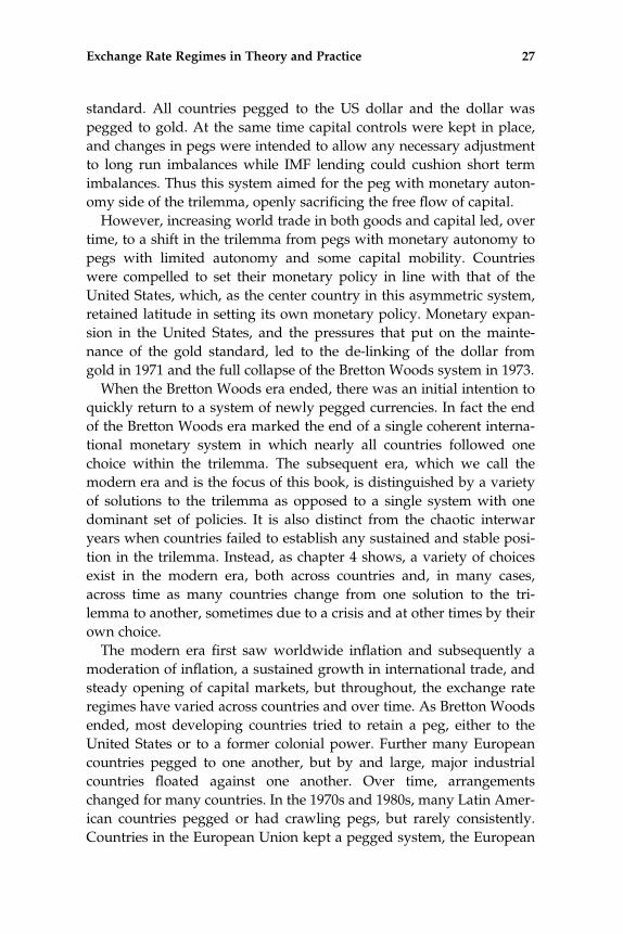
However, increasing world trade in both goods and capital led, over
time, to a shift in the trilemma from pegs with monetary autonomy to
pegs with limited autonomy and some capital mobility. Countries
were compelled to set their monetary policy in line with that of the
United States, which, as the center country in this asymmetric system,
retained latitude in setting its own monetary policy. Monetary expan-
sion in the United States, and the pressures that put on the mainte-
nance of the gold standard, led to the de-linking of the dollar from
gold in 1971 and the full collapse of the Bretton Woods system in 1973.
When the Bretton Woods era ended, there was an initial intention to
quickly return to a system of newly pegged currencies. In fact the end
of the Bretton Woods era marked the end of a single coherent interna-
tional monetary system in which nearly all countries followed one
choice within the trilemma. The subsequent era, which we call the
modern era and is the focus of this book, is distinguished by a variety
of solutions to the trilemma as opposed to a single system with one
dominant set of policies. It is also distinct from the chaotic interwar
years when countries failed to establish any sustained and stable posi-
tion in the trilemma. Instead, as chapter 4 shows, a variety of choices
exist in the modern era, both across countries and, in many cases,
across time as many countries change from one solution to the tri-
lemma to another, sometimes due to a crisis and at other times by their
own choice.
The modern era first saw worldwide inflation and subsequently a
moderation of inflation, a sustained growth in international trade, and
steady opening of capital markets, but throughout, the exchange rate
regimes have varied across countries and over time. As Bretton Woods
ended, most developing countries tried to retain a peg, either to the
United States or to a former colonial power. Further many European
countries pegged to one another, but by and large, major industrial
countries floated against one another. Over time, arrangements
changed for many countries. In the 1970s and 1980s, many Latin Amer-
ican countries pegged or had crawling pegs, but rarely consistently.
Countries in the European Union kept a pegged system, the European
Exchange Rate Regimes in Theory and Practice 27
Monetary System (EMS), but many broke or realigned pegs and others
stayed out of the system except for brief stints. Some countries have
consistently maintained a peg (e.g., Saudi Arabia) while others, such
as Argentina, have created a ‘‘harder’’ peg that mandates the peg by
law and requires adequate international reserve backing through a cur-
rency board. Some countries have even dispatched with their own
currency (e.g., Ecuador). Sets of other countries have joined in an
arrangement with a cross-national currency and single central bank, as
is the case with the initially eleven, but currently (at the time of this
writing) sixteen eurozone countries. Many countries have both pegged
and floated over the modern era. And pegging one bilateral rate does
not ensure overall exchange rate stability. Countries peg to a variety of
base currencies, so two countries that both peg, but to different bases,
might have an unstable bilateral exchange rate.
As we will see, nearly all countries have chosen to peg at some point,
and nearly all have chosen to float at some point. The characterization
of these exchange rate regimes, their dynamics, and the motivations
behind a government’s choice of its exchange rate regime are the focus
of the next three chapters of this book.
28 Chapter 2

3 Exchange Rate Regime Classifications
Everything should be made as simple as possible, but not simpler.
—Albert Einstein
Exchange rates are precisely measured. Exchange rate regimes are not.
The first challenge facing those who want to understand the character-
istics and consequences of exchange rate regimes is the identification
and implementation of a classification scheme. This scheme must de-
fine the categories that constitute an exchange rate regime and provide
a set of criteria that classifies a country’s experience in a particular time
period into one of those categories. These are far from trivial tasks, and
as Frankel has noted, ‘‘placing actual countries into those categories is
more difficult than one who has never tried it would guess.’’1
Exchange rate regime classification schemes vary along several
dimensions. A central dichotomy is between regimes declared by the
government, typically to the IMF (a de jure classification) and those
based on actual data (a de facto classification). These data will include
exchange rates, but may also include other variables, such as interest
rates or central bank reserves. Another distinction is the number of cat-
egories. Classification schemes may include only two broad categories
(e.g., ‘‘pegged’’ and ‘‘nonpegged’’), or a larger set of more narrowly
defined ones (e.g., ‘‘managed floating’’ and ‘‘limited flexibility’’). A
third consideration is the time period that constitutes one observation
for a country. Many schemes are based on behavior over a calendar
year, but one well-known system uses longer-run rolling averages.
This feature of a classification scheme will affect how frequently one
can observe switches from one category to another. The frequency of
switching is also determined by other rules used to categorize obser-
vations. For example, a one-time discrete devaluation could count as
a break in a pegged exchange rate, or it could be categorized as a

continuation of a fixed rate, albeit at a different peg before and after
the devaluation.
The range of issues that a classifications scheme must address sug-
gests that there is no one ‘‘correct’’ way to categorize exchange rate
regimes. Rather, those studying the characteristics or the consequences
of exchange rate regimes need to consider which classification scheme
is most appropriate for the question at hand. For example, a study of
the monetary constraints imposed by a fixed exchange rate, that is the
empirical relevance of the policy trilemma, would be best served by a
de facto classification that categorized exchange rates as fixed or float-
ing, and did not count a one-time discrete devaluation as a break in a
fixed exchange rate episode. A study of the length of peg episodes,
however, may be based on a system in which a break in a peg counts
as a floating exchange rate for that one year. Another type of study,
one that focuses on longer-lived regime behavior, may use categories
based on annual moving averages rather than yearly observations. Fi-
nally, one may want to consider data on reserves as well as that on ex-
change rates, and allow for a multiplicity of categories beyond ‘‘fixed’’
and ‘‘floating’’ in an analysis of the macroeconomic behavior of coun-
tries that intervene extensively but operate in an environment where
exchange rates are typically very volatile.
This chapter begins, in section 3.1, with a discussion of exchange rate
regimes reported by the IMF in its Annual Report on Exchange Arrange-
ments and Exchange Restrictions (EAER). This is considered the standard
de jure classification scheme, since the data were initially based on self-
reporting by governments. But, as discussed in section 3.1, these data
became a hybrid between a de jure and a de facto classification scheme,
beginning with the 1999 volume of EAER when the IMF began to aug-
ment government self-reported exchange rate arrangements with their
own staff’s evaluations. This was a response to the view that ‘‘the
authorities own descriptions of exchange rate regimes in the EAER is
patently inaccurate for some countries’’ (Fischer 2001, p. 4, n. 2). We
also show, in this section, the evolution in the categories used to clas-
sify exchange rate regimes in the EAER. This reflects the change in ex-
change rate arrangements during the modern era. It also highlights
some difficulties in comparing exchange rate regime categorization at
the time of the collapse of Bretton Woods in the early 1970s to subse-
quent experience.
Scholars outside of the IMF have undertaken their own efforts to
characterize exchange rate regimes, and we discuss a number of these
30 Chapter 3

de facto classification schemes in section 3.2. These classifications have
been used to investigate a range of issues in international macroeco-
nomics, and partly for that reason, the methods and data used across
them vary widely. The discussion in this section highlights this variety
and, in so doing, raises issues like the appropriate number of catego-
ries in a classification scheme and the data required to establish mem-
bership in a particular category. Of course, there is no one correct
answer concerning the number of categories or the data employed. In-
stead, the focus of the research influences the characteristics of the clas-
sification scheme.
The fact that the exchange rate classification schemes presented in
sections 3.1 and 3.2 differ does not mean that there are no overarching
results about exchange rate regimes in the modern era. Classification
schemes vary, and the extent of measured variation depends partly on
choices made in attempting to compare schemes with different num-
bers of categories. The practical question, however, is the extent of dif-
ferences, and similarities, across these classification schemes. We
address this question in section 3.3 by comparing and contrasting the
data from the various exchange rate regime classifications. This com-
parison will prove important as we consider the characterization of ex-
change rate regime behavior in the next chapter, and the consequences
of exchange rate regimes for economic performance in subsequent
chapters.
3.1 IMF Reporting of Exchange Rate Regimes
One way to determine a country’s exchange rate regime is simply to
ask its government what type of exchange rate system it has in place.
The International Monetary Fund does this in an ongoing manner. An-
nual reports that presented data from country surveys on exchange
rate arrangements and exchange restrictions have been published by
the IMF since 1950. These reports, titled Annual Report on Exchange
Arrangements and Exchange Restrictions, include narratives on member
states’ exchange rate systems (and exchange restrictions) as well as
tables that summarize this information.2
Table 3.1 shows the evolution of the exchange rate categories pre-
sented in the summary tables in volumes of the Annual Report on Ex-
change Arrangements and Exchange Restrictions from the 1973 volume
(reflecting exchange rate arrangements in 1972) until the 2006 volume.
As shown in this table, the 1973 volume, reflecting the arrangements in
Exchange Rate Regime Classifications 31

Table
3.1
AREARclassificationsover
time
1973Volume
1974–1987Volumes
1988–1996Volumes
Par
valueorcentral
rate
exists
Par
valueorcentral
rate
applied
Effectiverate
other
than
par
valueorcentral
rate
applicable
toallormost
tran
sactions
(a)fixed
rate
(b)fluctuatingrate
(c)peg
ged
rate
Specialrate(s)forsomeorallcapital
tran
sactionsan
d/orsomeorallinvisibles
Importrate(s)differentfrom
exportrate(s)
More
than
onerate
forim
ports
More
than
onerate
forexports
Exch
angerate
maintained
within
relatively
narrow
marginsin
term
sof
—USdollar
(197
4–87
)—
Sterling(197
4–19
87)
—French
fran
c(197
4–19
87)
—Groupofcu
rren
cies
(1974)
—Averag
eofexch
angeratesofmain
trad
ingpartners(197
4)—
Groupofcu
rren
cies
under
mutual
interven
tionarrangem
ents
(1975–1986
)—
Composite
ofcu
rren
cies
(197
5–87
)—
Australian
dollar,S.African
rand,
Span
ishpeseta(1977–1982)
—Set
ofindicators
(197
9–19
82)
Exch
angerate
notmaintained
within
relativelynarrow
marginsas
above
Specialexch
angerate
regim
eforsomeorall
capital
tran
sactions,invisibles
Importrate(s)differfrom
exportrate(s)
More
than
onerate
forim
ports
More
than
onerate
forexports
Exch
angeRatedetermined
onbasisofpeg
to —USdollar
(198
8–19
96)
—Poundsterling(1988–1995
)—
French
fran
c(198
8–19
96)
—Other
curren
cies
(1988–1996
)—
Composite
ofcu
rren
cies
(198
8–19
96)
Lim
ited
flexibilitywithresp
ectto
—single
curren
cy—
cooperativearrangem
ent
More
flexible
arrangem
ents
—ad
justed
accordingto
setofindicators
—other
man
aged
float
—indep
enden
tlyfloating
Specialrate(s)forsomeorallcapital
tran
s-actionsan
d/orsomeorallinvisibles
Importrate(s)differentfrom
exportrate(s)
More
than
onerate
forim
ports
More
than
onerate
forexports
32 Chapter 3

1997–1998Volumes
1999–2005Volumes
Peg
ged
to—
Single
curren
cy—
Composite
ofcu
rren
cies
Flexibilitylimited
More
flexible
arrangem
ents
—Man
aged
floating
—Indep
enden
tlyfloating
Exch
angerate
structure
—Dual
exch
angerates
—Multiple
exch
angerates
Exch
angerate
arrangem
ents
—Exch
angearrangem
entwithnoseparate
legal
tender
—Curren
cyboardarrangem
ent
—Conven
tional
peg
ged
arrangem
ent
—Peg
ged
exch
angerate
within
horizo
ntal
ban
ds
—Crawlingpeg
—Crawlingban
d—
Man
aged
float
withnoprean
nounced
pathfortheexch
angerate
—Indep
enden
tlyfloating
Exch
angerate
structure
—Dual
exch
angerates
—Multiple
exch
angerates
Exchange Rate Regime Classifications 33

the final full year of the Bretton Woods era, includes the two exchange
arrangement categories, ‘‘Agreed par value exists’’ and ‘‘Par value ap-
plied.’’ Par values were official exchange rates, usually in terms of US
dollars, that countries agreed upon with the IMF and had committed
to attempt to preserve. The countries that did not have a par value for
their currency were included in the category ‘‘Unitary effective rate,
not par value’’ (which had the subcategories ‘‘fixed rate,’’ ‘‘freely fluctu-
ating rate,’’ and ‘‘pegged rate’’), or in one of the four categories for mul-
tiple exchange rates (‘‘Special rate(s) for some or all capital transactions
and/or some or all invisibles,’’ ‘‘Import rate(s) different from export
rate(s),’’ ‘‘More than one rate for imports,’’ and ‘‘More than one rate for
exports’’).
The changes in the summary table categories between the 1973 and
the 1974 volumes reflect the end of the Bretton Woods era. With the
final collapse of the Bretton Woods system in March 1973, the term
‘‘par value’’ disappeared from these tables, and the ‘‘unitary effective
rate’’ category was dropped. The 1974 volume of the Annual Report on
Exchange Restrictions included two categories, ‘‘Exchange rate main-
tained within relatively narrow margins’’ and ‘‘Exchange rate not
maintained within relatively narrow margins.’’ This former category
was divided up into subcategories of the base currency or currencies,
including the US dollar, the British pound sterling, the French franc, a
group of other currencies, and an average of exchange rates of main
trading partners. These subcategories changed over time. The second
column of table 3.1 includes the list of bases and the years in which
they appeared in the summary tables.
While the end of the Bretton Woods system is widely viewed as her-
alding in the period of floating exchange rates, the view at the time, at
least as reflected in contemporary Annual Reports on Exchange Restric-
tions, gives a different perspective. An appendix to the 1974 volume
entitled ‘‘Central Rates and Wider Margins: A Temporary Regime—
Revised Decision’’ reflects the way in which the IMF, and many mem-
ber states, wrestled with the collapse of the Bretton Woods system.
That appendix states that the Fund called on members ‘‘to maintain a
satisfactory structure of exchange rates within appropriate margins
. . . during the temporary period preceding the resumption of effective
par values’’ (p. 19). An appendix to the 1975 volume of Annual Report
on Exchange Restrictions entitled ‘‘Guidelines for the Management of
Floating Exchange Rates’’ recommends that countries intervene in for-
34 Chapter 3
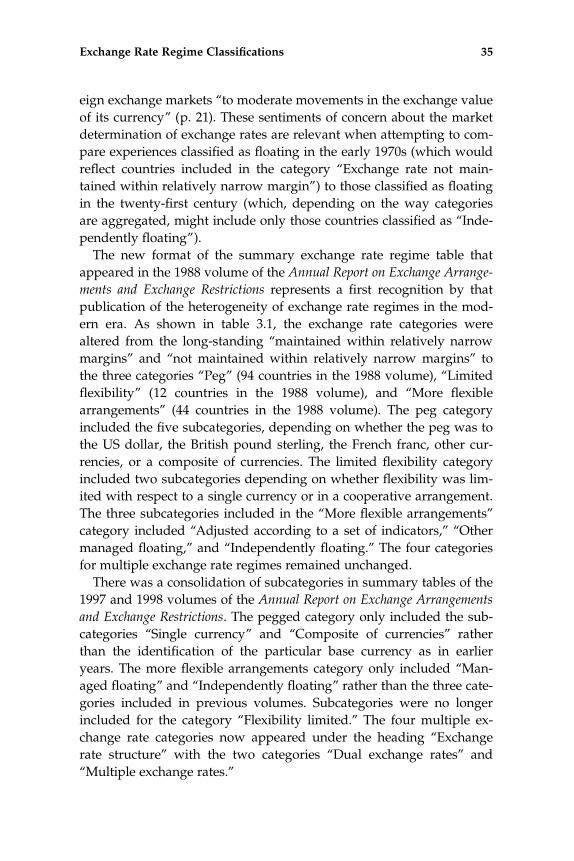
eign exchange markets ‘‘to moderate movements in the exchange value
of its currency’’ (p. 21). These sentiments of concern about the market
determination of exchange rates are relevant when attempting to com-
pare experiences classified as floating in the early 1970s (which would
reflect countries included in the category ‘‘Exchange rate not main-
tained within relatively narrow margin’’) to those classified as floating
in the twenty-first century (which, depending on the way categories
are aggregated, might include only those countries classified as ‘‘Inde-
pendently floating’’).
The new format of the summary exchange rate regime table that
appeared in the 1988 volume of the Annual Report on Exchange Arrange-
ments and Exchange Restrictions represents a first recognition by that
publication of the heterogeneity of exchange rate regimes in the mod-
ern era. As shown in table 3.1, the exchange rate categories were
altered from the long-standing ‘‘maintained within relatively narrow
margins’’ and ‘‘not maintained within relatively narrow margins’’ to
the three categories ‘‘Peg’’ (94 countries in the 1988 volume), ‘‘Limited
flexibility’’ (12 countries in the 1988 volume), and ‘‘More flexible
arrangements’’ (44 countries in the 1988 volume). The peg category
included the five subcategories, depending on whether the peg was to
the US dollar, the British pound sterling, the French franc, other cur-
rencies, or a composite of currencies. The limited flexibility category
included two subcategories depending on whether flexibility was lim-
ited with respect to a single currency or in a cooperative arrangement.
The three subcategories included in the ‘‘More flexible arrangements’’
category included ‘‘Adjusted according to a set of indicators,’’ ‘‘Other
managed floating,’’ and ‘‘Independently floating.’’ The four categories
for multiple exchange rate regimes remained unchanged.
There was a consolidation of subcategories in summary tables of the
1997 and 1998 volumes of the Annual Report on Exchange Arrangements
and Exchange Restrictions. The pegged category only included the sub-
categories ‘‘Single currency’’ and ‘‘Composite of currencies’’ rather
than the identification of the particular base currency as in earlier
years. The more flexible arrangements category only included ‘‘Man-
aged floating’’ and ‘‘Independently floating’’ rather than the three cate-
gories included in previous volumes. Subcategories were no longer
included for the category ‘‘Flexibility limited.’’ The four multiple ex-
change rate categories now appeared under the heading ‘‘Exchange
rate structure’’ with the two categories ‘‘Dual exchange rates’’ and
‘‘Multiple exchange rates.’’
Exchange Rate Regime Classifications 35
The most significant changes in the IMF reporting of exchange rate
arrangements since the collapse of Bretton Woods began with the 1999
volume of Annual Report on Exchange Arrangements and Exchange
Restrictions. First, and perhaps most important, reported exchange rate
arrangements were based on a database established by the IMF that
reflected its staff’s assessments of countries’ exchange rate policies
rather than just relying on the reports of governments. Second, the ‘‘Ex-
change rate arrangements’’ categories were completely revamped. As
shown in table 3.1, the eight new categories included ‘‘Exchange rate
arrangement with no separate legal tender,’’ ‘‘Currency board arrange-
ment,’’ ‘‘Conventional pegged arrangement,’’ ‘‘Pegged exchange rate
within horizontal bands,’’ ‘‘Crawling peg,’’ ‘‘Crawling band,’’ ‘‘Man-
aged float with no pre-announced path for the exchange rate,’’ and
‘‘Independently floating.’’ This structure of the summary table contin-
ues to the time of this writing.
The expansion of categories, from the two used from 1974 until 1987
that distinguished whether or not the exchange rate was ‘‘maintained
within relatively narrow margins’’ to the currently used eight catego-
ries, reflects the increasing heterogeneity of exchange rate arrange-
ments. This evolution of categories should bolster concerns about the
comparability of the IMF exchange rate regime statistics over time that
were raised above in the discussion on the early published views of the
desirability of floating exchange rates. Concerns about the comparabil-
ity of IMF exchange rate regime classification across time may also
arise because of the switch from a purely de jure system before 1999 to
a hybrid de jure and de facto system subsequently.
Despite these concerns, almost all research using exchange rate re-
gime classifications up until the mid-1990s were based on IMF report-
ing. Recently, however, this has changed with the development of a
number of de facto classification schemes. We next turn to a description
of these.
3.2 De facto Exchange Rate Regime Classifications
The decision by the IMF to verify governments’ stated exchange rate
regimes, beginning with the 1999 volume of the Annual Report on Ex-
change Arrangements and Exchange Restrictions, reflects the fact that
actual exchange rate behavior does not always matched proclaimed
intentions. For two decades after the collapse of Bretton Woods,
though, the de jure classification was the primary method researchers
36 Chapter 3
used to classify exchange rate behavior. This changed with the 1995 ar-
ticle ‘‘The Mirage of Fixed Exchange Rates’’ by Obstfeld and Rogoff. In
this article the authors argue that a consideration of actual exchange
rate behavior shows that few countries pegged for extended periods of
time. Calvo and Reinhart (2002) challenged de jure coding from the
opposite perspective. Their article, ‘‘Fear of Floating,’’ used data on
exchange rates, interest rates, and reserves to show that very few
countries that declared that their currencies floated actually allowed
for unfettered market determination of their exchange rates.
These articles highlight the need to examine de facto outcomes as
opposed to de jure claims. Neither, however, provides a systematic
classification of all potential country/year observations. In this section
we first consider some issues that arise when developing a de facto ex-
change rate classification scheme. We then discuss three well-known
exchange rate classification schemes.
3.2.1 De facto Classifications’ Characteristics
There are a few fundamental characteristics of any de facto exchange
rate classification scheme. One is the number of categories employed,
a consideration that also occurs with a de jure scheme. Other character-
istics, however, distinguish the construction of de facto schemes from
that of de jure schemes. These include the rules used to assign observa-
tions to one or another category, and the data employed to implement
these rules. In this section we address some issues on the characteris-
tics of de facto exchange rate classification schemes.
The central issue that characterizes any de facto exchange rate classifi-
cation scheme, or for that matter any de jure classification scheme, is
the number of categories employed. Comparisons of classification
schemes must address the comparability of these categories across
schemes. And, as we have seen, this issue is even raised when consid-
ering results from a single classification scheme if it changes over time.
The discussion in the previous section shows how the IMF de jure
scheme evolved from the early use of essentially two categories (main-
tained or not maintained within narrow margins) to the more recent
use of eight different categories. The wider range of categories allows
for finer gradations, but it is not clear that there is a straightforward
mapping that cleanly aggregates these newer categories into the
smaller set of earlier categories.3 This problem of comparability is even
more acute when attempting to compare results across classification
schemes.
Exchange Rate Regime Classifications 37
The assignment of each country/time period observation to a partic-
ular category in a de facto exchange rate classification scheme presents
another set of challenges, as noted in the quote by Jeffrey Frankel pre-
sented at the beginning of this chapter. The rules for assigning an ob-
servation to one category or another are not readily apparent when
there are a wide number of categories. For example, what are the prac-
tical, measurable, data-based differences that would place a country in
the category of ‘‘managed float’’ rather than ‘‘independently floating’’?
Even a seemingly straightforward bivariate classification scheme
presents challenges when one attempts to assign observations to the
two exhaustive categories, ‘‘pegged’’ and ‘‘not pegged.’’ Can a pegged
exchange rate move at all? Typically the answer is yes, and all of the
classification schemes discussed below allow for some exchange rate
movement in the ‘‘pegged’’ category. But how much can a pegged ex-
change rate move? In this case, history offers some guidance. Countries
that kept their exchange rate within roughly e2 percent bands have
been considered pegged, whether this range was for gold points dur-
ing the gold standard, for dollar exchange rates during the Bretton
Woods era, or for exchange rate bands around the central parity dur-
ing the EMS.
While the e2 percent rule seems to be clear, its implementation
raises the question of which exchange rate should be considered. Most
countries peg to a single base; in those cases the base country may be
determined through historical relationships or economic linkages. But
basket pegs—where a country pegs to an index of other currencies—
present a unique challenge. In most cases the weights in the basket
are not declared, making verification nearly impossible.4 Even when
weights are declared, or the IMF’s SDR (itself a basket) is the base,
many declared basket pegs are really direct pegs to an individual cur-
rency (see chapter 7 for more discussion of this point). Thus many de
facto classifications use an individual base regardless of whether the
declared base is a basket.5 Another consideration is the official ex-
change rate or, in countries with an important parallel exchange rate
market, the black market rate. Once again, the role of the use of the
classification scheme comes into play. The official rate may be the ap-
propriate choice if one wants to ask whether a government that said it
would peg its exchange rate actually kept its word. On the other hand,
one might consider the behavior of the black market rate if that is more
relevant for most transactions, and the focus of the analysis is the eco-
nomic impact of exchange rate stability.
38 Chapter 3
The data used to construct de facto exchange rate regime classifica-
tion schemes need not be limited to exchange rates. Some authors
(e.g., Levy-Yeyati and Sturzenegger 2003; Ghosh, Gulde, and Wolf
2002) argue that considering exchange rate data alone can lead to im-
proper regime classification, since the exchange rate reflects both
actions of the government and the underlying economic environment.
Thus some classification schemes use data on interest rates and
reserves to confirm that policy has had a hand in generating exchange
rate stability. This is meant to ensure that the observation of limited ex-
change rate movement reflects a policy of a peg rather than merely a
quiescent environment that has not put any pressure on the exchange
rate to move. A problem with this approach, however, is that a per-
fectly credible exchange rate peg that is never challenged by the mar-
ket may not require any government intervention, and therefore no
reserve or interest rate responses. At the same time reserves and inter-
est rates can move for many reasons, and their volatility may not re-
flect an effort to peg the exchange rate to the exclusion of other policy
goals.
How important is the concern that spurious exchange rate stability
leads to misclassifying regimes as pegs when in fact they just happen
to look that way? One answer to this question draws on some results
presented in Calvo and Reinhart (2002). They note that the probability
that the bilateral exchange rate had a monthly change of less than 2.5
percent was roughly 60 to 70 percent during classic floats like the US
dollar/DM rate, the US dollar/yen rate or the US dollar/Australia dol-
lar rate. In these cases the probability of twelve straight months of
changes smaller than 2.5 percent (in either direction) is between 0 and
1 percent. In addition, if a classification requires the tighter restriction
of staying within the same e2 percent bands at all times during the
year, the odds of a spuriously coded peg drop further. These statistics
suggest that reserve or interest rate data are not vital in order to ensure
against spuriously coding quiescent periods as a pegs.
A final consideration concerns moments of transition from one
pegged rate to another. For example, suppose there is a one-time dis-
crete devaluation of a currency. The exchange rate is pegged both be-
fore and after the devaluation. It is not really accurate to say that the
exchange rate ‘‘floated’’ at the moment of the devaluation. On the other
hand, the devaluation does mark a change from one exchange rate to
another. As in other cases discussed above, the proper coding of this
episode depends on the question addressed. One may want to count
Exchange Rate Regime Classifications 39

the year in which the devaluation occurs as a continuation of the peg if
the exchange rate classification scheme is being used to address the
link between the exchange rate and monetary autonomy. A study of
the effects of a pegged exchange rate on trade, however, might find it
more useful to distinguish the year in which a devaluation takes place
from other years in which the exchange rate is pegged. In any event,
the importance of this issue means that we will highlight how this fea-
ture of exchange rate behavior is coded in the classifications discussed
below.
3.2.2 A Taxonomy of De facto Classifications
In this section we provide details on three influential and widely
used de facto exchange rate classification schemes; those developed by
Levy-Yeyati and Sturzenegger (2003), Reinhart and Rogoff (2004), and
Shambaugh (2004). Each of these schemes was first used in an article
published in a major scholarly journal, and each has been subsequently
used extensively by other researchers.6 The research question posed by
each article differs and, partly for this reason, the resulting classifica-
tion schemes also differ from each other in terms of the number and
definition of categories and the assignment rules. The discussion below
provides some context for the classification schemes by referring to the
focus of the research that it was developed to address. This discussion
highlights a point raised above, that choices made about particular
attributes of an exchange rate regime classification scheme reflect its in-
tended use.
Levy-Yeyati–Sturzenegger One of the first attempts to generate a de
facto classification in recent years is due to the work of Eduardo Levy-
Yeyati and Federico Sturzenegger in their article ‘‘To Float or Fix: Evi-
dence of the Effects of Exchange Rate Regimes on Growth,’’ which was
published in the September 2003 issue of the American Economic Review.
The motive for their development of a de facto exchange rate classifica-
tion scheme is that ‘‘the de jure classification based on the regime the
governments claim to have in place . . . ignores the fact that many
alleged floats intervene in the exchange market to reduce exchange
rate volatility, while some fixers devalue periodically to accommodate
independent monetary policies’’ (p. 1175, emphasis in original).
While the title of this article suggests a bivariate classification, the
Levy-Yeyati–Sturzenegger (hereafter LYS) scheme includes three cate-
gories; pegged, intermediate, and float. Assignment into these catego-
40 Chapter 3

ries is based on cluster analysis using data on the change in the ex-
change rate, the volatility of the change in the exchange rate, and the
change of reserves relative to a monetary aggregate. A year in which a
country has low exchange rate volatility but large reserve volatility is
categorized as pegged observation. A country that has a year in which
there is a relatively constant (though nonzero) rate of change in the ex-
change rate and a high rate of change in reserves is categorized as an
intermediate observation, as is a country with moderate volatility
across all variables. A year in which a country has a high level of ex-
change rate volatility but a low level of reserve volatility is scored as a
year of floating. A fourth category in the LYS scheme is called ‘‘incon-
clusive.’’ Country–year observations are considered inconclusive in
the cluster analysis when there is a constant exchange rate with low re-
serve volatility. Observations in this category are subsequently reclas-
sified as pegged if there is no change in the exchange rate or, when
there is a declared peg, the exchange rate moves by only a small
amount.
The appeal of the LYS strategy is its emphasis on actual behavior
over declared intentions. In addition, by analyzing the rate of change
of the exchange rate and the reserves volatility, the LYS scheme sepa-
rates countries that have crawling pegs or heavily managed exchange
rates from other nonpegged countries. LYS do not view the exchange
rate as sufficient information to separate pegs and floats, but instead
combine exchange rate behavior with evidence of deliberate interven-
tion. LYS, though, require intervention to take the form of changes
in foreign reserves and draw no distinction between sterilized and
unsterilized intervention. A country can maintain a pegged exchange
rate without ever changing its reserves if it is willing to change its
money supply or interest rates, and a country that changes reserves
dramatically may not really be showing concrete commitment to its ex-
change rate peg if all intervention is sterilized. In addition highly un-
stable M2 may make the reserve ratio volatile even if there is little or
no intervention. LYS state that theory suggests highly variable reserves
for a country that is truly pegged, but if a country maintains its ex-
change rate by constantly changing its interest rate as, for example,
Bahrain does, there will be no change in reserves. One could argue
that such a country is exhibiting a much stronger commitment to
its exchange rate than a country that continually exercises sterilized
intervention—changing reserves but unwilling to allow its domestic
money supply to be changed in defense of the exchange rate.
Exchange Rate Regime Classifications 41

This problem becomes clear when one examines the countries that
are originally listed as inconclusive by the cluster analysis. Countries
such as Bahrain, the Bahamas, or Hong Kong, that have very strong
fixed exchange rates against the dollar are not listed as pegged in the
first round or even the second round of their exercises. This is because
their reserves are not highly volatile; they simply adjust their money
supply at all times to avoid the need for intervention, or they are so
trusted in their regime that they are rarely challenged. The subsequent
decision to code zero percent change countries picks up many of those
left out but omits some undeclared de facto pegs. On the other hand,
countries that intervene dramatically but break their peg, such as Ire-
land in the EMS crisis, or float but have sufficient reserves volatility,
such as New Zealand, are listed as fixed. The LYS coding does not,
however, include most years with a discrete devaluation from one
fixed rate to another as a peg year because the change in the exchange
rate relative to the change in reserves volatility is gauged as being too
large to be a peg in those cases.
This system of classification was a large advance over simply relying
on the de jure codes and has a number of appealing features. It tries to
address intent as well as exchange rate behavior, and it tries to sepa-
rate countries into three groups. This methodology can be quite useful
for trying to separate countries that are dirty floats or that are heavily
managed. On the other hand, it is not entirely transparent in that it
does not yield a clear picture of what it means to be a peg or a float.
There is no clear dividing line, but instead a combination of factors
contributes to the decision. Furthermore the categorization of some
observations as pegs after the cluster analysis classification rounds
shows that the statistical methodology cannot itself pick up all the
pegged countries. The methodology also codes significantly more pegs
than other classifications (59 percent of observations are coded as pegs
compared to a maximum of 46 percent in the other classifications). Fi-
nally, the data burden (requiring reserves as well as exchange rate
data) makes the classification unavailable for many country/year
observations.
Reinhart–Rogoff Carmen Reinhart and Kenneth Rogoff created an
exhaustive coding of exchange rate regimes that is largely based on
the behavior of parallel, market-determined exchange rates. They pres-
ent this classification scheme in ‘‘The Modern History of Exchange Rate
Arrangements: A Reinterpretation’’ that was published in the February
42 Chapter 3

2004 issue of the Quarterly Journal of Economics. They use this coding to
reconsider experience with exchange rate regimes in the post–World
War II period. For example, they argue that ‘‘Very frequently—
roughly half the time for official pegs—we find that dual/parallel rates
have been used as a form of ‘backdoor’ floating, albeit one usually
accompanied by exchange controls’’ (p. 2). Thus they contend that de
facto floating was very common during the Bretton Woods period.
They also argue that after pegs, crawling pegs were the most common
exchange rate arrangement during the modern period.
The ‘‘fine grid’’ version of the classification scheme includes fourteen
categories, and the ‘‘coarse grid’’ aggregates these into five categories.7
Of particular note is the inclusion of the separate coarse grid ‘‘Freely
falling’’ category. This represents instances where depreciation is rapid
and sustained and where inflation is high. Roughly 10 percent of
all observations are included in this category (roughly 15 percent of all
nonpegged observations). Reinhart and Rogoff argue that the inclu-
sion of the ‘‘Freely floating’’ episodes in a broader floating category
muddies efforts to discern differences in economic performance across
categories.
Observations are assigned to categories based on the odds of the
parallel (not official) exchange rate being outside a band over a five-
year rolling window. The authors argue that the parallel rate best dem-
onstrates the true stance of the government and that any classification
system that fails to distinguish between a unified rate system and one
with parallel rates is ‘‘fundamentally flawed.’’ They also state that par-
allel and dual exchange rates were widely prevalent and ‘‘enormously
important not only in developing countries but in virtually all the Eu-
ropean countries up until the late 1950s, and sometimes well beyond’’
(p. 2).
The five-year rolling window represents an effort to avoid spurious
switches in exchange rate regimes due to devaluations or brief periods
of volatility (or brief periods of quiescence). This strategy makes it dif-
ficult to directly compare this classification scheme with those based
on annual data, since the Reinhart–Rogoff classification for a country
in a particular year may not match the behavior of that country in that
year if it changes regimes frequently. This strategy also implies that a
country that pegs sporadically may be classified as a crawling peg
throughout the sample when, in truth, it pegs in some years and floats
in others. Such behavior might be one source of the prevalence of
crawling pegs in this classification system. A third implication of the
Exchange Rate Regime Classifications 43

use of a rolling window is that it allows for far fewer switches in
regimes, and consequently lengthier peg and float spells because it
smoothes over some transitions.
In some ways the Reinhart–Rogoff classification merges information
on capital controls and exchange rate regimes (a point alluded to in
their QJE article and one also discussed in Shambaugh 2004). A coun-
try that has a constant official exchange rate but a volatile black market
rate is likely one that has stabilized its official rate via controls on trad-
ing or other capital control mechanisms. Such a country may have a
plausibly fixed official exchange rate, but will not be coded as such in
Reinhart–Rogoff because the parallel rate is not constant.
The Reinhart–Rogoff classification scheme is best suited for analyses
that focus on transactions, especially if those transactions tended to
take place at the black market rate, which, they argue, ‘‘is often the
most economically meaningful rate’’ (p. 2). On the other hand, this
classification scheme may be less well suited for studies of central
bank commitments made, since countries make no attempt to stabilize
the black market rate. When Malaysia institutes capital controls to de-
fend its peg (and presumably the black market rate moves away from
the peg), a researcher would have to determine whether this still repre-
sents a peg, since the country claims to have maintained its fixed ex-
change rate and in fact the official rate has not budged, or whether the
capital controls represent a deviation from pegging.
Shambaugh Jay Shambaugh created an exchange rate regime classifi-
cation scheme in the spirit of that presented by Obstfeld and Rogoff
(1995) to consider the empirical relevance of the policy trilemma. The
first work using this classification scheme was his article ‘‘The Effect of
Fixed Exchange Rates on Monetary Policy’’ published in the same Feb-
ruary 2004 issue of the Quarterly Journal of Economics as the Reinhart–
Rogoff article. The results in the article show that the monetary policies
of countries with pegged exchange rates were significantly linked to
the monetary policies of the base country to which they pegged, while
there was no significant link between the monetary policies of coun-
tries that did not peg and the monetary policies of the respective large
countries that would be the most likely base country in a pegged
system.
Unlike the other two exchange rate regime classification schemes
described above, the Shambaugh classification is bivariate and assigns
annual country/year observations into either a peg or a nonpeg cate-
44 Chapter 3

gory. The assignment is based on whether the official exchange rate
stays within a e2 percent band against the base currency. The base
country is the currency to which a country pegs or would peg if it
were pegging.8 This means that a truly multilateral basket peg, one
that is not merely a veil for a de facto single currency peg, may not be
categorized as a peg if it has no true base.9 Like Reinhart–Rogoff, this
classification relies only on the exchange rate to code observations. Un-
like Reinhart–Rogoff, it is the official exchange rate, not a parallel rate
that is used, because government policies affect the official rate. While
it only used the exchange rate volatility to code observations, the clas-
sification required two years of staying within a e2 percent band to
ensure that no observations that randomly lacked volatility were spuri-
ously coded as pegs.
One benefit of this classification scheme is that it allows for relatively
straightforward modification in order to best address particular re-
search questions. For example, Obstfeld, Shambaugh, and Taylor
(2008) add a third category, soft pegs, which are exclusive from hard
pegs. Soft pegs represent observations where the exchange rate stays
within e5 percent bands, but not within e2 percent bands. Impor-
tantly, under this classification scheme, classic floats, such as the US
dollar against the yen or the deutsche mark, are never classified as
soft pegs, which should reduce concerns that countries that allow a
fair bit of flexibility are accidentally classified as soft pegs rather than
nonpegs.
The original Shambaugh classification scheme does not record a one-
time realignment as a break in a peg. This is consistent with his re-
search question, since theory suggests that the exchange rate regime
continues to restrict monetary policy when there is a one-time discrete
devaluation to a new peg. In practical terms, the rule that was used
was that any exchange rate that had a percentage change of zero in
eleven out of twelve months is considered fixed.10 In a modified ver-
sion of this classification scheme developed to consider the characteris-
tics of fixed and floating exchange rate spells, Klein and Shambaugh
(2008) do not count an observation with a discrete devaluations as a
peg since this would artificially raise the persistence of pegs (see chap-
ter 4).
Single-year pegs were dropped in the original Shambaugh (2004)
classification scheme to ensure that an observation of a stable exchange
rate reflects government policy rather than just a quiescent environ-
ment. But, in another example of modifying the classification scheme
Exchange Rate Regime Classifications 45

to make it appropriate for the research question, Klein and Shambaugh
(2008) include single-year pegs in order to gauge more accurately the
length of spells of pegged exchange rates. The original Shambaugh
(2004) scheme that eliminates single-year pegs automatically limits the
minimum length of pegs to two years. As discussed in the next chap-
ter, there is fairly good evidence that nearly all single-year pegs are in
fact legitimate pegs and do not reflect a spurious lack of volatility.
The original Shambaugh coding scheme, as well as its modified ver-
sions, is fairly straightforward. It also has the virtue of matching our
basic intuition of the properties of a fixed exchange rate since a country
is categorized as pegged if its exchange rate stays relatively stable. The
use of official exchange rate data allows for wider coverage and easier
updating than a classification system requiring parallel rates, or data
on interest rates and central bank reserves. Of course, the trade-off
here is that this classification system may not be the most appropriate
for countries for which the official exchange rate is not the most eco-
nomically relevant. But, for those countries where the official exchange
rate is economically relevant, this system also has the advantage of an
annual frequency which matches up well with variables typically used
in studies that investigate the effect of exchange rate regimes on trade,
monetary policy, and so forth.
3.3 Correlation of Different Exchange Rate Regime Classifications
The previous two sections present four exchange rate classification
schemes with different sets of categories and widely different methods
for assigning observations to these categories. As discussed, one reason
that there is such variety in these classification schemes is that each
was developed to address different questions. Still it is reasonable to
expect a fair amount of agreement across these schemes, since at their
core they all represent efforts to capture the same behavior. In this sec-
tion we investigate whether in fact this agreement exists.
A comparison of these exchange rate regime classifications requires a
mapping of categories across schemes. The common denominator, so
to speak, is the distinction between pegged and nonpegged exchange
rate regimes, since the Shambaugh classification includes only these
two categories. Thus we will compare the results across classification
schemes by compressing the categories in the IMF coding, the LYS
scheme, and the Reinhart–Rogoff classification system into this binary
set. We define the categories of pegs, limited flexibility, and coopera-
46 Chapter 3

tive arrangements in the IMF coding as pegged regimes, and the
other categories constitute the nonpegged category. The Levy-Yeyati-
Sturzenegger scheme includes a pegged and a floating category, and
we include the intermediate category in the set of observations coded
as nonpegged for the purposes of this comparison. The set of pegged
exchange rates for the Reinhart–Rogoff classification system is the first
coarse grid category,11 which consists of the four fine grid categories
‘‘No separate legal tender,’’ ‘‘Preannounced peg or currency board ar-
rangement,’’ ‘‘Preannounced horizontal band that is narrower than or
equal toe2 percent,’’ and ‘‘De facto peg.’’
Table 3.2 presents the percentage of observations for which binary
versions of each classification scheme agree with one another.12 The
statistics in this table show that the results from the four classification
schemes are broadly similar. The degree of agreement varies between
73 and 86 percent. This is clearly better than random (where the
expected degree of agreement is 50 percent), but there is still a fair
amount of disagreement. The biggest distinctions are between the LYS
scheme and both the IMF and the Reinhart–Rogoff classifications.
Also, as shown in the bottom row of the table, the LYS scheme codes
observations as pegs far more often than the other three schemes,
while the Reinhart–Rogoff codes observations as pegs far less often.
As discussed in the previous section, the LYS scheme generates more
peg observations, since reserve volatility can lead to an observation
being recorded as a peg even if the exchange rate moves considerably.
Alternatively, in most cases large discrete devaluations or revaluations
will be considered floats in LYS as the exchange rate volatility will
dominate the reserves volatility, but these observations are often
Table 3.2
Percentage agreement of various pegged and nonpegged coding methodologies
IMF LYS RR Shambaugh
IMF 100%
LYS 74% 100%
RR 81% 73% 100%
Shambaugh 86% 80% 82% 100%
Pegged 41% 58% 33% 45%
Note: Shown are percentages of observations where different codings yield the sameresult as one another. All coding is collapsed to a binary peg and nonpeg coding. Thelast row shows the share of observations which are coded as peg by each classification.Years: 1973–2004.
Exchange Rate Regime Classifications 47
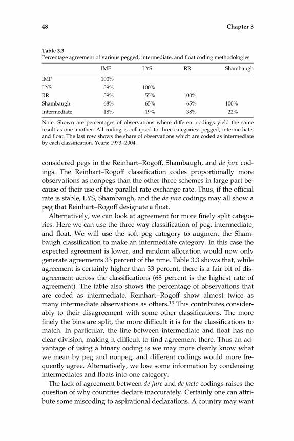
considered pegs in the Reinhart–Rogoff, Shambaugh, and de jure cod-
ings. The Reinhart–Rogoff classification codes proportionally more
observations as nonpegs than the other three schemes in large part be-
cause of their use of the parallel rate exchange rate. Thus, if the official
rate is stable, LYS, Shambaugh, and the de jure codings may all show a
peg that Reinhart–Rogoff designate a float.
Alternatively, we can look at agreement for more finely split catego-
ries. Here we can use the three-way classification of peg, intermediate,
and float. We will use the soft peg category to augment the Sham-
baugh classification to make an intermediate category. In this case the
expected agreement is lower, and random allocation would now only
generate agreements 33 percent of the time. Table 3.3 shows that, while
agreement is certainly higher than 33 percent, there is a fair bit of dis-
agreement across the classifications (68 percent is the highest rate of
agreement). The table also shows the percentage of observations that
are coded as intermediate. Reinhart–Rogoff show almost twice as
many intermediate observations as others.13 This contributes consider-
ably to their disagreement with some other classifications. The more
finely the bins are split, the more difficult it is for the classifications to
match. In particular, the line between intermediate and float has no
clear division, making it difficult to find agreement there. Thus an ad-
vantage of using a binary coding is we may more clearly know what
we mean by peg and nonpeg, and different codings would more fre-
quently agree. Alternatively, we lose some information by condensing
intermediates and floats into one category.
The lack of agreement between de jure and de facto codings raises the
question of why countries declare inaccurately. Certainly one can attri-
bute some miscoding to aspirational declarations. A country may want
Table 3.3
Percentage agreement of various pegged, intermediate, and float coding methodologies
IMF LYS RR Shambaugh
IMF 100%
LYS 59% 100%
RR 59% 55% 100%
Shambaugh 68% 65% 65% 100%
Intermediate 18% 19% 38% 22%
Note: Shown are percentages of observations where different codings yield the sameresult as one another. All coding is collapsed to three categories: pegged, intermediate,and float. The last row shows the share of observations which are coded as intermediateby each classification. Years: 1973–2004.
48 Chapter 3

to peg and even very briefly try, but not seriously commit to it, leading
to a de jure peg but de facto float. However, there are many disagree-
ments that persist, including many long-run pegs that are not declared.
Alesina and Wagner (2006) investigate why some countries behave
more restrictively than they declare, or vice versa, and find that coun-
tries with weak institutions tend to declare pegs but fail to maintain
them while those with strong institution frequently have tighter de facto
regimes than they declare. Genberg and Swoboda (2005) discuss rea-
sons why a government may peg an exchange rate without declaring
that as its goal, which suggests that de jure declared regimes may not
really represent the true goals or actual intent of a government. Thus a
country that fixes despite declaring a float is not necessarily breaking a
commitment, but trying to send a particular signal.
The lack of agreement across de facto exchange rate classification
schemes may be viewed as an indication of an inability of these
schemes to accurately code country behavior.14 As this discussion
shows, however, disagreements often stem from efforts to address
different questions. Thus these differences are not simply a difference
in measuring pegs, but a difference in defining them.15 The Klein–
Shambaugh classification measures direct peg spells to consider the
length of peg spells and float spells. Shambaugh (2004) measures an-
nual coding of exchange rate behavior based on well-established band
criteria as well as allowing discrete devaluations so as to prevent artifi-
cially breaking up a consistent regime in an effort to test the monetary
policy implications of pegging. Reinhart–Rogoff’s classification both
smoothes over time to determine regimes as opposed to spells and
uses the black market rate—hence merging both exchange rate choices
and capital control choices in an effort to consider the implications of
policy regime choices broader than that of the choice of peg or float
alone. Levy-Yeyati and Sturzenegger use reserves behavior in addition
to exchange rate behavior to better distinguish intermediate spells
from float spells, while possibly allowing somewhat volatile but heav-
ily managed exchange rates to be considered pegs. Thus the classifica-
tion scheme one may choose depends on the question posed; those
interested in whether a country is pegged and stable in a given year
may use the Shambaugh classification scheme, those interested in
absolute stability of the peg may choose the Klein–Shambaugh cod-
ing, those interested in overarching policy regimes smoothed over
time could choose to refer to the Reinhart–Rogoff coding, and those
exploring intermediates versus floats or intervention behavior may
refer to LYS.
Exchange Rate Regime Classifications 49
3.4 Conclusion
Exchange rate classification is neither a simple nor a trivial task. Cata-
loging behavior that runs across a broad spectrum into discrete catego-
ries requires some sort of rule and will invariably occasionally divide
countries that behave somewhat similarly into different bins. At the
same time, any tests that compare outcomes across regimes will in-
herently depend on categorizing the observations properly. Different
techniques provide different insights into the exchange rate regime
behavior of countries, and their disagreements should not simply be
viewed as one being right or wrong. We will typically use the Sham-
baugh classification (or one of its modifications, depending on the re-
search question) as our core classification. An advantage of such a
procedure, as opposed to looking at relative volatility benchmarks is
that this definition of a peg (within a 2 percent band) is clear, invariant
over time, and matches the historical definitions of pegs such as the
gold points in the gold standard, the bands in Bretton Woods and the
EMS. The coding is also available for nearly all years due to its lesser
data requirements. Other classifications may be useful, though,
depending on the research question.
50 Chapter 3
4 The Dynamics of Exchange Rate Regimes
Because things are the way they are, things will not stay the way they are.
—Bertolt Brecht
The economic consequences of the choice of an exchange rate regime,
as outlined in chapter 2, represent one of the classic lines of inquiry in
international finance. As discussed in chapter 3, with the advent of the
modern era, a wide set of experiences with exchange rate regimes
emerged. These experiences over a four-decade time period offer a rich
tableau for investigating the effects of exchange rate regimes on trade,
growth, stability, and other economic outcomes. But these inquiries
are partially predicated on the durability of countries’ exchange rate
regimes.1 For example, it is difficult to imagine fixed exchange rates
having an impact by anchoring expectations if they break so frequently
that people do not take them seriously, or if they are so fleeting that
they have no consequences for more persistent variables like inflation
or trade flows.
In this chapter we investigate the dynamic behavior of exchange rate
regimes. We present data on the duration of both fixed exchange rate
regimes and flexible exchange rate regimes. We also go beyond this
static analysis and discuss the prevalence of flipping from a fixed ex-
change rate regime to a flexible exchange rate regime, and then back
to a fixed exchange rate regime. This dynamic analysis is important for
a complete characterization of exchange rate regimes in the modern
era.
The analysis presented in this chapter challenges the simple view
that a country is either a ‘‘fixer’’ or a ‘‘floater.’’ This was a reasonable
characterization of most countries during the gold standard period,
and even in the Bretton Woods period. The modern era has, however,

included much more switching than in these earlier periods. For exam-
ple, almost half of the fixed exchange rate episodes that appear in the
main data set used in this chapter do not last more than two years. In
a similar fashion there are also a large number of short-lived floating
exchange rate episodes. The prevalence of these short-lived fixed and
floating episodes means that switching is common.
This is not to say, however, that the modern era is an anarchic period
where the terms ‘‘fixed’’ and ‘‘floating’’ have ceased to be relevant. A
central result presented in this chapter is that the expected duration of
a peg increases dramatically if it survives past two years. Conse-
quently, at any one time the set of countries that are pegged includes a
large proportion of those with a peg lasting for a relatively long dura-
tion. Similarly, the set of floating exchange rate episodes includes a
large number of short-lived episodes and a smaller number of coun-
tries with persistently floating exchange rates.
The existence of a significant number of stable, meaningful exchange
rate regimes runs counter to some recent influential research. The title
of the article by Obstfeld and Rogoff, ‘‘The Mirage of Fixed Exchange
Rates’’ (1995), reflects their conclusion that long-lived currency pegs
are rare and only found among small countries. They write ‘‘literally
only a handful of countries in the world today have continuously
maintained tightly fixed exchange rates against any currency for five
years or more’’ (p. 87).2 On the other side of the ledger, Calvo and
Reinhart (2002) argue that many countries whose governments claim
that they allow their currencies to be determined by market forces
actually intervene in currency markets to manage exchange rates, a be-
havior that gives the title to their article ‘‘Fear of Floating.’’
One reason that the ‘‘mirage’’ of fixed exchange rates and govern-
ments’ ‘‘fear of floating’’ resonated with the research community is
that these results seem to accord with strands of earlier research that
found little role for exchange rate regimes in determining major macro-
economic and aggregate outcomes beyond the real exchange rate.3 An
important initial contribution in one line of research is the work of
Baxter and Stockman (1989). They show that there is no significant dis-
tinction in terms of consumption variability or the variability of GDP
growth between the experience of countries that had fixed exchange
rate regimes and those that had floating exchange rate regimes when
using de jure codes to mark different exchange rate regimes. Another
strand of research failed to uncover a strong effect of exchange rate
variability (and, implicitly, of exchange rate regimes) on bilateral inter-
52 Chapter 4
national trade flows.4 The Obstfeld–Rogoff and Calvo–Reinhart results
were viewed as consistent with these results; why would the exchange
rate regime matter for macroeconomic outcomes, or even for the direc-
tion and size of trade flows, if pegs are but a ‘‘mirage’’ and if flexible
regimes are not really characterized by floating exchange rates? Thus
the message from these two lines of research, one that considers the ex-
change rate experience with exchange rate regimes and the other that
examines the effects of exchange rate regimes on economic perfor-
mance, is that exchange rate regimes are largely inconsequential.
Much of the rest of this book takes issue with these points of view.
Recent research, discussed in later chapters, has found a large number
of economic outcomes that vary across exchange rate regime. In this
chapter we lay some of the groundwork for this subsequent discussion
by analyzing the dynamic behavior of exchange rate regimes. We
begin in the next section by defining an exchange rate spell and pre-
senting the distributions of fixed exchange rate spells and floating
exchange rate spells. We show that these distributions are similar,
with both having a large number of short-lived spells and a smaller
number of long-lived spells. An important implication is the flipping
of pegged rates, that is, the end of a peg is often followed by the re-
formation of a new peg. Section 4.2 then presents a statistical analysis
of the duration of flexible and fixed exchange rate spells that considers
the likelihood of the continuation of a spell for another year, condi-
tional on its survival up to that point. This characterization of the
dynamics of exchange rate regimes in the modern era offers a different
picture than either the classic stability that marked earlier eras or what
one would expect from the results claiming that fixed exchange rates
are merely a ‘‘mirage.’’
4.1 Fixed, Floating, and Flipping Exchange Rate Regimes
The basic unit of observation for the analysis of the dynamics of ex-
change rate regimes in this chapter is a spell. We consider two types of
spells, a fixed spell and a floating spell. A fixed spell represents one or
more consecutive years during which the exchange rate stays within a
narrow range in each year (e2 percent from one month to the next, as
well as e2 percent over the course of a year). A floating spell repre-
sents one or more consecutive years during which the exchange rate
does not stay within that narrow range in any of the years of the spell.
Both fixed exchange rate spells and floating exchange rate spells are
Dynamics of Exchange Rate Regimes 53

characterized by the number of years they last. The distributions of the
durations of fixed and floating exchange rate spells represent the num-
ber of spells of each level of annual duration, from one year up
through the full span of thirty-two years, since the data set covers the
years 1973 to 2004.
This e2 percent rule recalls the de facto Shambaugh classification
scheme described in the previous chapter. The main classification
scheme used in this chapter is, in fact, a modified version of that classi-
fication scheme, one used in Klein and Shambaugh (2008). In this
scheme, as in the Shambaugh scheme, a country is classified as having
a pegged exchange rate in a particular year if its official exchange rate
against the appropriate base country stays within a e2 percent band
both from one month to the next as well as over the entire year. The
two differences between the Klein–Shambaugh scheme and the Sham-
baugh scheme described in chapter 3 are that the former allows for
one-year pegs, and it also counts a one-time realignment as a break in
a peg. We include single-year pegs to avoid artificially increasing the
durability of pegs. Had we only classified pegs as observations that
had limited exchange rate movements for two or more years, we
would have pegs look strikingly more persistent.5 Similarly, we view
realignments as breaks in a peg to prevent falsely inflating the durabil-
ity of pegs.
Table 4.1 presents some basic statistics for the exchange rate regime
data based on the Klein–Shambaugh classification scheme.6 This data
set represents the experience of 125 countries over the period 1973 to
2004.7 We classify the 21 countries that were members of the OECD in
1973 as the subset of industrial countries. Of the 3,924 country–year
observations in this data set, 48 percent are pegs.8 Pegs are more prev-
alent among developing countries than among industrial countries,
with 49 percent of the developing country–year observations repre-
senting pegs but only 39 percent of the industrial country–year obser-
vations representing pegs. There are 793 exchange rate spells, with 395
floating spells and 398 peg spells. The mean duration of peg spells is
4.7 years, and the mean duration of float spells is 5.2 years. These
means are greater than the respective median durations, which are 2
years for both peg spells and float spells.
The fact that the means of the duration of both peg spells and float
spells are much larger than their respective medians suggests that both
distributions are skewed to the right. The histograms of these distribu-
tions, presented in figures 4.1 and 4.2, confirm this. These histograms
54 Chapter 4
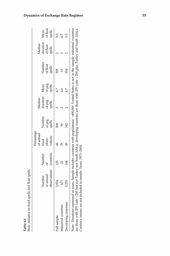
Table
4.1
Basicstatistics
onfixed
spellsan
dfloat
spells
Number
ofan
nual
observations
Number
of
countries
Percentage
ofan
nual
fixed
obser-
vations
Number
ofpeg
spells
Med
ian
duration
ofpeg
spells
Mean
ofpeg
spells
Number
offloat
spells
Med
ian
duration
offloat
spells
Mean
offloat
spells
Fullsample
3,924
125
4839
82
4.7
395
25.2
Industrial
countries
671
2139
562
4.6
613
6.7
Dev
elopingcountries
3,253
104
49342
24.7
334
25.0
Note:Durationsexpressed
inyears.Sam
ple
includes
countrieswithpopulations>400,000.
United
Statesis
notin
thesample;industrial
countries
arethose
withIFScode<20
0butnotTurkey
norSouth
Africa;
dev
elopingcountriesarethose
withIFScode>20
0plusTurkey
andSouth
Africa.
Curren
cyunionsarenotincluded
insample.Years:19
73–20
04.
Dynamics of Exchange Rate Regimes 55
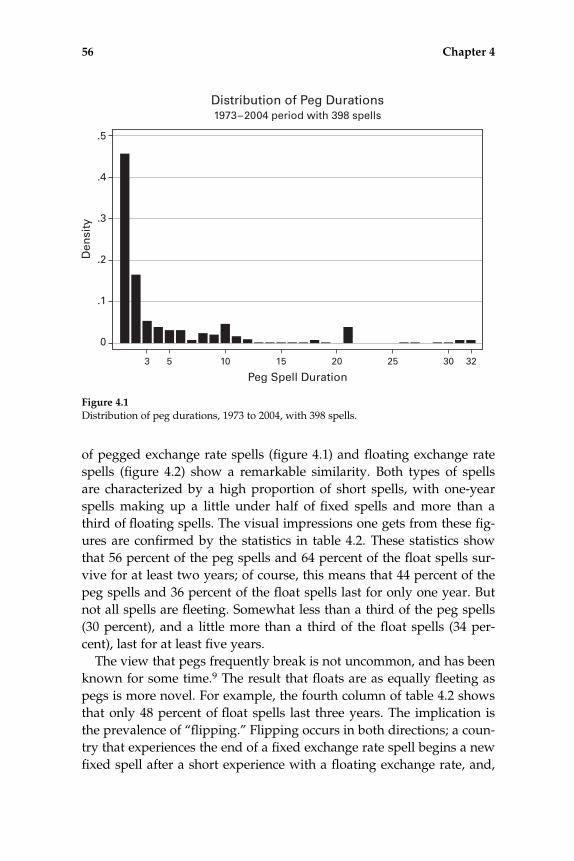
of pegged exchange rate spells (figure 4.1) and floating exchange rate
spells (figure 4.2) show a remarkable similarity. Both types of spells
are characterized by a high proportion of short spells, with one-year
spells making up a little under half of fixed spells and more than a
third of floating spells. The visual impressions one gets from these fig-
ures are confirmed by the statistics in table 4.2. These statistics show
that 56 percent of the peg spells and 64 percent of the float spells sur-
vive for at least two years; of course, this means that 44 percent of the
peg spells and 36 percent of the float spells last for only one year. But
not all spells are fleeting. Somewhat less than a third of the peg spells
(30 percent), and a little more than a third of the float spells (34 per-
cent), last for at least five years.
The view that pegs frequently break is not uncommon, and has been
known for some time.9 The result that floats are as equally fleeting as
pegs is more novel. For example, the fourth column of table 4.2 shows
that only 48 percent of float spells last three years. The implication is
the prevalence of ‘‘flipping.’’ Flipping occurs in both directions; a coun-
try that experiences the end of a fixed exchange rate spell begins a new
fixed spell after a short experience with a floating exchange rate, and,
Figure 4.1
Distribution of peg durations, 1973 to 2004, with 398 spells.
56 Chapter 4

Figure 4.2
Distribution of float durations, 1973 to 2004, with 395 spells.
Table 4.2
Fixed spell and float spell survival statistics, by spell
Peg spells Float spells
Allcountries Industrial
Devel-oping
Allcountries Industrial
Devel-oping
At least 2 years 56% 56% 56% 64% 73% 63%
At least 3 years 40% 33% 42% 48% 54% 47%
At least 4 years 35% 33% 35% 38% 42% 38%
At least 5 years 30% 33% 30% 34% 37% 33%
>5 years 28% 33% 27% 30% 32% 30%
Total spells 365 55 310 365 59 306
Note: Sample includes countries with populations >400,000. United States is not inthe sample; industrial countries are those with IFS code <200 but not Turkey nor SouthAfrica; developing countries are those with IFS code >200 plus Turkey and South Africa.Currency unions are not included in sample. Years: 1973–2004.
Dynamics of Exchange Rate Regimes 57

in a similar fashion, a country may have a short experience with a fixed
exchange rate between two floating exchange rate spells. This view,
that many countries flip back and forth in their exchange rate arrange-
ments, differs from the conventional view that most countries are char-
acterized as being ‘‘fixers’’ or ‘‘floaters.’’ It also importantly contrasts
with crisis models which describe the end of a pegged exchange rate,
but not what follows that collapse. Our results suggest that crises are
simply part of the evolution of the exchange rate regime, and that a re-
peg following a crisis is quite likely.
A country might flip from a peg to a float and back to a peg again
because of an inability to maintain a consistent exchange rate regime.
But if this inability to maintain a consistent policy was pervasive, we
would expect to find relatively few instances of long-lived spells. The
statistics presented in table 4.3, which presents the longest peg dura-
tion and the longest float duration for each of the 125 countries in the
sample, shows that this is not the case. As shown in that table, a large
number of countries maintain at least one fairly long-lived peg and at
least one fairly long-lived float episode in the modern era. Almost 70
percent of the countries in the sample have peg spells of four or more
years, and 70 percent have float spells of five or more years. Of course,
we cannot know the intentions of the 12 percent of countries that either
never peg or have no peg spells that last more than one year, or those
of the 20 percent of countries that either never float or have no float
spell that lasts for more than one year. It seems unlikely, however, that
Israel could not peg for more than one year (its maximum peg is one
year) or that Syria could not float for more than one year (its maximum
Table 4.3
Longest fixed and float episodes (by country)
Length Pegs Length Floats
0 7 6% 0 3 2%
1 8 6% 1 22 18%
2 19 15% 2 5 4%
3 6 5% 3 7 6%
4 7 6% 4 0 0%
5þ 78 62% 5þ 88 70%
This table shows the distribution of the longest peg and float episodes by country. Thereare 125 countries included. For example, 7 countries never peg, 6 have a longest peg of 3years, and 78 have one of 5 years or more; 3 never float, and 88 float for 5 or more consec-utive years at some point in the sample. Years: 1973–2004.
58 Chapter 4
float is one year). Rather, these outcomes seem to reflect policy choices.
Similarly, Canada never pegged for more than two years at a time, but
certainly other large industrial countries (e.g., France, which has stayed
within its EMS bands every year since 1987) have been able to do so.
The result reported in table 4.3, that 78 countries (out of 125) had a
peg of at least five years, seems to be at odds with the view that pegs
are, in the words of Obstfeld–Rogoff (1995), a ‘‘mirage.’’ And while
some of the statistics presented in table 4.2 support the notion that
pegs are short lived, for example the fact that over 70 percent of fixed
spells in the modern era have not lasted for more than five years, this
statistic also means that a substantial proportion do last for an
extended period. This contrasts with the ‘‘remarkably small’’ (p. 87)
number of durable pegs identified by Obstfeld–Rogoff, who list only
six ‘‘Major Economies with Open Capital Markets’’ that successfully
maintained a peg for at least five years at the time they wrote their ar-
ticle in June 1995 (these countries are Austria, Hong Kong, Luxem-
bourg, the Netherlands, Saudi Arabia, and Thailand).10
How is it that over a quarter of our sample of 365 fixed rate spells,
including almost a third of the sample of 55 fixed rate spells from in-
dustrial countries, have a duration of more than five years while
Obstfeld–Rogoff (1995) present only a ‘‘handful’’ of spells with this du-
ration? One reason is a difference in samples, since we include some
countries omitted by Obstfeld–Rogoff who considered them too small,
in terms of population, to include in their analysis. The more important
reason, however, concerns the timing of their study. Their statistics on
the duration of fixed exchange rates are based on a snapshot of experi-
ence of the duration of fixed exchange rates at one particular date, June
1, 1995. This was a distinctive moment since many long-standing pegs
had ended within the previous few years in the wake of the 1992 EMS
crisis, the 1994 Tequila crisis, and the 1994 devaluation of the CFA
countries against the franc. In fact their article was partly motivated by
these events.
After 1995, many of the countries that saw their pegged exchange
rates break reestablished new fixed rates. As a result there were just as
many long-lived pegs in 2000 as there were in 1990. Thus the time
when Obstfeld–Rogoff conducted their analysis was a low point for
long-lived fixed exchange rates. This is demonstrated in figure 4.3.
This figure shows that 1994 to 1998 was the low point of long-lived
pegs with only an average 17 in those years (out of roughly 125 coun-
tries in the sample)11 as compared to 36 long-lived pegs in 2000 and an
Dynamics of Exchange Rate Regimes 59

average of 32 long-lived pegs in the modern era.12 Thus a focus on ex-
change rate pegging since 1973, rather than the situation in 1995, and
on peg spells, rather than countries, alters the impression one has of
the durability of exchange rate pegs.
The results reported so far are based on the Klein–Shambaugh de
facto exchange rate regime classification scheme. We close this section
by offering some results that are based on the other classification
schemes. As we will see, differences in spell statistics across classifica-
tion schemes reflect differences in the way these classification schemes
are constructed, as discussed in detail in the previous chapter.
Table 4.4 presents statistics of exchange rate spells that are created
through the use of the Reinhart–Rogoff, Shambaugh, and IMF classifi-
cation schemes discussed in chapter 3.13 Spells for the Reinhart–Rogoff
and IMF schemes are constructed by mapping the respective multiple
categories into a bivariate fixed/float classification.14 This table also
reproduces the spell statistics based on the Klein–Shambaugh classifi-
cation scheme that are presented in table 4.1 to facilitate comparisons
across all four schemes.
Figure 4.3
Figure shows the number of countries in a peg that has lasted for five or more yearsat that moment. The panel is roughly balanced with between 122 and 125 countries inthe sample. Currency unions are eliminated from the sample with the exception ofspells that began as pegs and converted to currency unions (which include some EMUobservations).
60 Chapter 4

Table
4.4
Statisticsonfixed
spellsan
dfloat
spellsacross
classifications
Annual
obser-
vations
Countries
insample
Peg
obser-
vations(%
)Peg
spells
Peg
med
ian
Peg
mean
Float
spells
Float
med
ian
Float
mean
Fullsample
RR
3,20
210
434
.01
918
11.82
107
2020
.31
JS3,92
412
546
.02
199
59.16
191
711
.09
DJ
3,92
412
542
.03
167
59.69
148
14.5
15.17
KS
3,92
412
547
.53
398
24.67
395
25.21
Industrial
countries
RR
671
2131
.74
1610
.513
.00
2025
24.00
JS67
121
35.62
316
7.55
365.5
12.00
DJ
671
2141
.23
218
12.52
2023
20.10
KS
671
2139
.34
562
4.63
613
6.67
Dev
elopingcountries
RR
2,531
8334.61
758
11.57
8720
19.46
JS3,25
310
448
.17
168
59.46
155
810
.88
DJ
3,25
310
442
.19
146
59.28
128
1414
.40
KS
3,25
310
449
.22
342
24.68
334
24.95
Note:RR¼
Reinhart–Rogoff
coding;JS
¼Sham
bau
gh
coding;DJ¼
IMFdejure
coding;KS¼
Klein–Sham
bau
gh
coding,reproducingstatistics
from
table
4.1.
Years:19
73–20
04.
Dynamics of Exchange Rate Regimes 61

Table 4.4 shows that all four classifications have comparable num-
bers of country–year observations. There is a big distinction, however,
in the number of spells identified. The fewest number of spells are gen-
erated by the Reinhart–Rogoff coding, and the most by the Klein–
Shambaugh coding. The relatively small number of spells based on the
Reinhart–Rogoff coding is a consequence of their use of a five-year roll-
ing window, rather than purely annual observations, as discussed in
chapter 3. An implication of this is that spells based on the Reinhart–
Rogoff classification scheme have much longer duration than those
based on the other three schemes, with the median durations of eight
years for peg spells and twenty years for float spells. The IMF ex-
change rate regime classification scheme results in the next fewest
number of spells, and the next longest average durations. This reflects
an aspect of the de jure classification; countries often do not change the
declaration of their exchange rate regime, even if pegs break and re-
form, or if pegs are intermittent. The median durations of fixed and
float spells based on the Shambaugh classification scheme are also
longer than those based on the Klein–Shambaugh classification
scheme, since it does not count the switch from one parity to another
as a break in a fixed exchange rate spell, and it also requires that pegs
last for more than one year.
This is an important example where the fact that different classifica-
tions may generate different results does not mean the results are not
robust. Instead, it emphasizes the importance of picking a classification
that is appropriate to the question being studied. For example, trying
to analyze the switching in and out of exchange rate regimes with the
Reinhart–Rogoff classification would not make sense as they are delib-
erately trying to smooth over switches to look at longer run episodes
rather than spells.
4.2 Survival of Fixed and Floating Exchange Rate Spells
Tables 4.1 and 4.2 report the mean and median durations of fixed and
floating exchange rate spells, and the proportions of spells that last for
at least a certain number of years. These statistics provide an overview
of the characteristics of spells. They do not, however, offer the most
useful information for people who want to know the likely perma-
nence of a fixed exchange rate over a time horizon that may be relevant
for many economic decisions. For example, if someone in a country
with a dollar peg has signed a contract for purchasing goods from the
62 Chapter 4
United States, and the contracted price is in dollars, that person would
want to know the likelihood that the specific dollar peg still holds at
the time in the future when the goods are delivered and payment is
made. While the median and mean lengths of fixed exchange rate
spells offer some guidance along these lines, a better gauge of the like-
lihood of the continuation of that peg takes into account other informa-
tion, including the number of years that the peg has already been in
effect and, perhaps, features of the peg relationship (e.g., the base
country) and characteristics of the pegging country itself (e.g., whether
it is an industrial country).
The previous section provided us with simple odds that did not uti-
lize all the information an economic agent would have. Those are un-
conditional probabilities. The common thread running through all
three sets of results in this section is the conditioning of probabilities of
the continuation of a fixed or floating exchange rate spell. These condi-
tional probabilities offer views of peg and float spells that more closely
reflects how economic agents who must make decisions at a particular
moment view the likely permanence of a peg, or the continuation of a
policy of allowing the exchange rate to float.
We begin by presenting statistics on the likelihood of switching from
a peg to a float, or vice versa, at different time horizons. These statistics
offer a different perspective on the duration of pegs and floats than that
afforded by the results presented in the previous section. We then dis-
cuss the likelihood that an existing fixed exchange rate peg lasts for
one more year, and the chance that a country that has been allowing
its currency to float will continue to do so for another year. We show
that these probabilities change with the number of years already spent
in a fixed or floating exchange rate spell, respectively, through the use
of duration analysis. Duration analysis provides estimates of the condi-
tional likelihood of the continuation of a spell as a function of the num-
ber of years the spell has already run.15
4.2.1 Rates of Switching
We first consider the likelihood of an economy being in a fixed spell or
a floating spell at a particular moment, conditional on whether it had a
pegged or a floating exchange rate at different times prior to that mo-
ment. Table 4.5 reports that the probability of a country having a fixed
exchange rate in year t, if it had a fixed exchange rate in the previous
year, is 82 percent. (Of course, this implies that the chance a peg
breaks, or of having a floating exchange rate conditional on having a
Dynamics of Exchange Rate Regimes 63

Table
4.5
Probab
ilityofsw
itch
ingsp
ellstatenextyear,an
dofremainingin
samesp
ell1,
3,or5years
infuture,an
nual
data
Years
a
All
countries
Industrial
Dev
eloping
Years
a
All
countries
Industrial
Dev
eloping
FloatðtÞ
jPegðt�1Þ
18%
17%
19%
Peg
ðtÞjFl
oatðt�1Þ
17%
13%
18%
Peg
ðtÞjPe
gðt�1Þ
82%
83%
81%
FloatðtÞ
jFloatðt�1Þ
83%
87%
82%
Peg
ðtÞjPe
gðt�3Þ
66%
71%
65%
FloatðtÞ
jFloatðt�3Þ
65%
70%
64%
Peg
ðtÞjPe
gðt�5Þ
55%
62%
54%
FloatðtÞ
jFloatðt�5Þ
54%
61%
52%
Note:Sam
ple
includes
countrieswithpopulations>400,000.
TheU.S.is
notin
thesample;industrial
countriesarethose
withIFScode<20
0but
excludeTurkey
and
South
Africa;
dev
elopingcountriesarethose
withIFScode>20
0plusTurkey
and
South
Africa.
Curren
cyunionsarenot
included
inthesample.Sam
plesbeg
inin
1973
andareupthrough20
03forthenextyear’sconditional
probab
ilities,upthrough20
01for3years’
hen
ceconditional
probab
ilities,
and1999
for5years’hen
ceconditional
probab
ilities.
Countriesmust
remainin
samestatecontinuously;that
is,
Peg
ðtÞjPe
gðt�3Þ
signifies
stay
ingpeg
ged
inðt�3Þ,ðt�2Þ,ðt�1Þ
andðtÞ
.Countriesthat
flip
inan
doutofastateareconsidered
tohav
ebroken
thestate.
a.Years
inpeg
spellorin
float
spells.
64 Chapter 4

fixed exchange rate in the prior year is 100 percent� 82 percent ¼ 18
percent.) The comparable probability of having a floating exchange
rate in a given year, conditional on having a float in the prior year, is
83 percent. This suggests both fixed and floating exchange rate regimes
are fairly durable. This persistence is also evident if we consider the
probabilities of having a fixed exchange rate given that there was a
fixed exchange rate three or five years before (and no switching in be-
tween), since these probabilities are 66 percent and 55 percent, respec-
tively. The comparable probabilities for floating exchange rates are
almost the same, at 65 percent and 54 percent. While these probabilities
are somewhat higher for industrial countries than for developing coun-
tries in all cases, the differences are not pronounced.16
At first, one might be surprised by the high levels of persistence of a
state of pegging or floating, given the unconditional probabilities pre-
sented in the previous section that show that nearly half of the peg
spells and more than a third of float spells end after their first year.
The difference across these two sets of statistics reflects the fact that
the conditional statistics in table 4.5 are based on annual cross sections
rather than spells. Long-lived spells are given a bigger weight when
calculating these annual cross sections than when calculating spell-
based statistics. This insight is especially important when considering
analyses of exchange rate regimes’ effects on growth or other variables.
Such studies typically involve annual observations, and therefore they
will draw more observations from a single long peg spell than from a
number of shorter duration spells. Indeed, even though the results in
table 4.2 show that flipping back and forth between fixed spells and
floating spells is common, the statistics in table 4.3 suggest that coun-
tries do stay in longer duration spells with some regularity, giving rise
to the results in table 4.5 that show that there is substantial continuity
in the persistence of exchange rate regimes from one year to the next,
or even from one year to three or five years hence. Thus, rather than
looking at how long a newly started peg will last (looking at spells),
we are asking that if we randomly took any pegged country right
now, what are the odds the peg lasts one year more (or three or five).
4.2.2 Conditional Survival Rates
The continuity in exchange rate spells evident from table 4.5 is based
on statistics on the likelihood that a country maintains a fixed or float-
ing spell conditional on being in that respective type of spell in a pre-
vious year. People have more information than this, however. In
Dynamics of Exchange Rate Regimes 65

particular, they know how long a peg spell or a float spell has been in
effect. They can use this information to gain a more precise estimate of
the likelihood of the continuation of a spell for one more year, given its
survival up to that moment.
The conditional survival rate of a spell represents the probability
that a spell that has survived through year (t� 1) still is in effect at the
end of year t. Figure 4.4 presents these survival rates for fixed ex-
change rate spells and for floating exchange rate spells at the horizons
of two through six years (since, by definition, all spells last for at least
one year). The statistics in this table show that 56 percent of the fixed
exchange rate spells last for at least two years. This, of course, matches
the statistic in presented in table 4.2. Of the 56 percent of the fixed ex-
change rate spells that last for at least two years, 71 percent last for a
third year, and of the 40 percent (¼ 56 percent � 71 percent) of spells
that last for at least three years, 86 percent last for at least a fourth
year. These conditional survival rates are somewhat higher for floating
exchange rate spells.
The pattern of conditional survival rates for both fixed and floating
exchange rate spells is similar in that both are increasing with the num-
ber of years already spent in the spell. This represents positive duration
dependence (which is also called a decreasing hazard rate, as discussed
below). The longer a peg has been in place, the greater is the likelihood
Figure 4.4
Conditional survival rates of peg and float spells.
66 Chapter 4

that it will survive for one more year. If these conditional survival rates
decreased with the number of years already spent in a spell, this would
represent negative duration dependence (or an increasing hazard rate). As it
is, the statistics in figure 4.4 show that people should increase their
estimates that a peg will survive for one more year as its duration
increases. Even though almost half of all pegs do not survive to a sec-
ond year, once a peg has been in existence for three years there is a
very strong chance (greater than 85 percent) that it will last for a fourth
year. The result is similar for floating exchange rate spells. Thus, once a
fixed or a floating exchange rate regime has even a small bit of history,
as little as three years, it is quite likely to last through any single given
subsequent year.
4.2.3 Hazard Functions
The discussion of conditional survival rates shows that spells may be
more durable depending how long they have been in existence. That
is, they exhibit duration dependence. A way to estimate the duration
dependence of a set of spells, and to see how duration dependence
shifts with variables other than the time spent on a peg, is through the
use of a hazard function. In this context a hazard function, h(t), repre-
sents the likelihood that a fixed exchange rate spell that has lasted up
until year t� 1 ends in year t when the currency begins to float, or
alternatively, the likelihood that a floating exchange rate that has
lasted up until year t� 1 switches to a peg in year t. A decreasing haz-
ard, h0(t) < 0, represents positive duration dependence, an increasing
hazard, h0(t) > 0, represents negative duration dependence, and a con-
stant hazard, h0(t) ¼ 0, represents constant duration dependence.17
The duration dependence of a set of spells based on the estimate of a
hazard function compliments the conditional survival rates discussed
above. In addition one can estimate the role of covariates—that is, vari-
ables other than time spent in a spell—on duration dependence. In this
case the arguments of the hazard function include the vector of covari-
ates, x, as well as the time spent in the spell, t.
A commonly used function in duration analysis is the Weibull hazard
function. This function takes the form
h(t, x; l, b) ¼ lt(l�1) exp(xb) (4.1)
where t is the time in the spell, and x is vector of covariates that shift
the hazard function. The parameter l in the baseline Weibull hazard
Dynamics of Exchange Rate Regimes 67
function lt(l�1) and the vector of coefficients associated with the covari-
ates, b, are estimated by a maximum likelihood method.
The baseline hazard function lt(l�1) is decreasing in t if l < 1 and, in
this case, exhibits positive duration dependence. Conversely, it exhibits
negative duration dependence if l > 1. The baseline hazard is invariate
to the time already spent in the spell, and exhibits constant duration
dependence, if l ¼ 1.
Covariates shift the baseline Weibull hazard function without alter-
ing its duration dependence. A positive coefficient bi means that larger
values of its associated covariate xi increases the hazard function; that
is, larger values of xi makes it more likely that a spell will end in
period t, given its survival to period (t� 1).
We investigate the effect of several covariates. One covariate is a
dummy variable identifying which fixed exchange rate spells and
which floating exchange rate spells are those of industrial countries.
Another covariate, used only for fixed exchange rate spells, is whether
the base country is the United States. A third covariate, for both fixed
exchange rate spells and floating exchange rate spells, is the length of
the immediately preceding spell.18 A positive value of the coefficient
associated with the length of the immediately preceding float spell in
an estimate of the peg spell hazard function implies that a shorter pre-
vious float is associated with a lower subsequent peg spell hazard; that
is, peg spells tend to last longer if the immediately preceding float
spells are shorter (as we have seen, a high proportion of float spells
last for only one year). Also, a positive value of the coefficient associ-
ated with the length of the immediately preceding peg spell in an esti-
mate of the float spell hazard function implies that longer peg spells
are associated with shorter subsequent float spells.
Results of estimating the Weibull hazard function for fixed exchange
rate spells, and also estimating it for floating exchange rate spells, are
presented in table 4.6. The estimated value of l is 0.84 for fixed ex-
change rate spells, and this estimate is significantly less than 1.00 at
the 95 percent level of confidence. Likewise the estimated value of l is
0.91 for floating exchange rate spells and is significantly less than 1.00
at the 95 percent level of confidence. This confirms the statistical
robustness of the conditional survival functions presented above that
show that both fixed exchange rate spells and floating exchange rate
spells become more durable over time—they exhibit positive duration
dependence.19
68 Chapter 4

The estimates presented in table 4.6 show that the coefficient on the
previous float spell is positive and significant for peg spells, and the
coefficient on the previous peg spell is positive and significant for float
spells. This suggests that short float spells are associated with longer
subsequent peg spells (since the hazard is lower) and that long peg
spells are associated with shorter subsequent float spells. Thus a long
peg that breaks tends to flip back to pegging relatively quickly. Finally
the results in this table also show that pegs to the US dollar have a
higher hazard rate, ceteris paribus, than pegs to other bases.20
4.3 Re-forming Pegs
We emphasize the re-formation of pegs, but a highly relevant question
is ‘‘at what exchange rate?’’ That is, do pegs simply loosen and then re-
tighten around the same central band, or are they re-formed at a new
level? Table 4.7 examines this question. There are 398 peg spells in
table 4.1, and we use the same sample (1973–2004, 125 countries)
described there. Sixty-four peg spells are still in existence in 2004,
which leaves us with 334 peg breaks to examine. Of these, 210 have re-
formed into a new peg within five years.21 The table shows the ex-
change rate change from the pegged year to the following year after
the break for these 210 observations. We use the annual average ex-
change rate, so we do not look at the exchange rate in the year of the
break, since exchange rate pegs that broke toward the end of the year
will appear to have no associated change in the level of the exchange
rate. We see that the average exchange rate has moved considerably
Table 4.6
Estimates of Weibull conditional hazard functions
Peg spells Float spells
CoefficientStandarderror Coefficient
Standarderror
Previous spell 0.033** (0.011) 0.047** (0.014)
Industrial country 0.256 (0.190) 0.211 (0.175)
US base dummy 0.650** (0.135)
l 0.844** (0.034) 0.912* (0.041)
Number of spells 397 332
Note: * significant at 95% level of confidence, **at the 99% level for null hypothesis ofb ¼ 0 for covariates and null hypothesis of l ¼ 1 for baseline hazard function parameter.
Dynamics of Exchange Rate Regimes 69

Table
4.7
Exch
angerate
beh
aviorafterapeg
endsuntilitreform
s
Chan
gein
theexch
angerate
from
peg
ged
yearto
year
afterthepeg
break
s
Spells
Averag
ech
ange
25th
percentile
Med
ian
75th
percentile
Peg
break
s33
487
%1%
13%
49%
Chan
gein
theexch
angerate
bytimepeg
isreform
ed
Reform
after
Spells
Averag
ech
ange
25th
percentile
Med
ian
75th
percentile
Ban
ds
overlap
Ban
ds
dep
reciate
Ban
ds
appreciate
1year
103
50%
0%14
%60
%14
%71
%16
%
Immed
iate
3869
%18
%86
%10
0%0%
89%
11%
Other
1year
6538
%0%
6%17
%22
%60
%18
%
2years
5453
%�1
%15
%47
%9%
70%
20%
3years
2913
5%12
%32
%46
%7%
7%17
%
4years
1261
%2%
18%
102%
17%
67%
17%
5years
1213
3%29
%72
%20
0%8%
92%
0%
Note:Thefirstrow
showstheexch
angerate
beh
aviorafterapeg
ends.
Subsequen
trowsshow
theexch
angerate
chan
gebythetimeapeg
has
reform
edas
wellas
wherethenew
ban
dsliewithresp
ectto
theold
exch
angerate
ban
dswhen
thepeg
reform
s.Threeextrem
eoutliers
areexcluded
from
theav
erag
es.
70 Chapter 4

(87 percent) after the break of a peg.22 The median country has depreci-
ated by 13 percent, with a quarter of countries not having depreciated
at all the year after the peg breaks, and another quarter having depreci-
ated by a full 50 percent or more.
Subsequent rows show the number of peg spells that have re-formed
after a given amount of time, the change in the exchange rate by that
time, and, in the last three columns, whether the new bands overlap
the old ones or are more depreciated or more appreciated than the
original peg bands. There are 103 peg spells that re-form after just one
year. Thirty-eight of these are immediate realignments where there is a
change in the exchange rate outside thee2 percent bands in only the
month of the realignment itself.23 Eighty-nine percent of these 38 dis-
crete realignments are to a new, substantially depreciated exchange
rate; the median depreciation is 86 percent. For the other 65 pegs that
re-form with only a year break, the median depreciation is only 6 per-
cent, and 22 percent of the spells have re-formed at bands that overlap
the old ones. Thus, a fair number of peg breaks are outside their 2 per-
cent bands for only a year and the new peg is reasonably close to the
old one.
Pegs that re-form at longer horizons tend to do so at a significantly
depreciated exchange rate. The 75th percentile change in the exchange
rate by the time the peg has re-formed is near a 50 percent depreciation
for pegs that re-form after two or three years, and is above 100 percent
for pegs that re-form after four or five years. The average depreciations
are also in the range of 50 percent to more than 100 percent at these
horizons, even when we exclude two outliers when calculating these
statistics.
The results in table 4.7 show that the restoration of a peg can occur
with a very large change in the exchange rate. Thus, in some cases, a
new peg restores stability, but people who had made long-run deci-
sions based on the old pegged rate now face a substantially more
depreciated one. Still, nearly 10 percent of the pegs that re-form within
five years do so at a rate close to the old bands, and around 20 percent
of these re-peg at a more appreciated rate.
In the end, analyzing the end of peg spells without considering that
they re-form is incomplete, but, at the same time, just because a peg
re-forms does not mean that it does so at a rate close to its old value.
Even though stability returns with a new peg (at least for a short time,
anyway), in at least half the cases there is a fairly substantial depre-
ciation, and in about a quarter of the cases there is a very substantial
depreciation.
Dynamics of Exchange Rate Regimes 71

4.4 Conclusion
In chapters 8 through 11 we will discuss recent research that shows
substantial effects of the exchange rate regime on trade and a variety
of macroeconomic outcomes. These results seem inconsistent with the
perception that pegs do not really peg and floats do not really float,
that is, that exchange rate regimes do not matter for the exchange rate,
let alone other outcomes. In this chapter we find that, despite the fact
that many peg spells break soon after they begin, a fair number last be-
yond five years. These longer spells are overrepresented in an annual
cross section, as compared to short spells. In addition, once a peg lasts
longer that a year or two, the probability that it will continue for one
more year, conditional on lasting up until that year, rises dramatically.
The implication is that the length of a particular peg is more important
than the less specific knowledge of average peg duration for agents
considering actions that are affected by the maintenance of the peg.
We also show that float spells have properties similar to those of peg
spells, especially with respect to the prevalence of many short duration
spells. This shows that many countries re-form pegs quickly after expe-
riencing the end of a peg spell.
A second issue, however, is whether there are significant and impor-
tant quantitative differences in exchange rate volatility across exchange
rate regimes. The mere classification of annual observations into those
categorized as ‘‘pegs’’ and those categorized as ‘‘floats’’ (or, more accu-
rately, nonpegs) would not matter if the ‘‘fear of floating’’ truly limited
exchange rate flexibility when countries do not peg. As discussed in
the chapters 6 and 7, the existence of these differences has been subject
to some debate. But we will show that the magnitude of bilateral ex-
change rate volatility between a country that has a pegged rate and its
base country is quite distinct from bilateral volatility when a country
does not peg.24 Countries that peg have lower multilateral volatility as
well, mainly because these countries tend to avoid extreme bilateral
volatility outcomes.25
72 Chapter 4

5 The Empirics of Exchange Rate Regime Choice
To peg or not to peg, that is the question.
—Heard somewhere in Denmark
Governments make a wide range of decisions on economic policy.
Some of these decisions represent a set of institutional choices that are
made infrequently, such as the development or modification of statutes
governing the operation of a central bank. Other choices are made
more often, as a response to immediate concerns; for example, the pas-
sage of a short-run fiscal stimulus package to counter an economic
downturn. In both cases it is also important to recognize that decisions
are typically not made by the ‘‘benevolent social planner’’ of economic
theory, rather economic choices often reflect political struggles among
several competing interest groups.
One of the key economic decisions facing any government is its
choice of exchange rate regime. But is this a choice based on deep
structural economic and political features that tend to not change
much over time? And, if so, which of these factors are most important?
Or, instead, does the choice of the exchange rate regime in a particular
year mainly reflect current economic and political conditions? These
questions are the focus of this chapter.
The nature of the question of exchange rate regime choice is different
in the modern era than in earlier times. The choice of whether to partic-
ipate in the gold standard was bound up with the choice of whether to
be engaged in the broader international monetary system. This had
implications for international trade, since participation in the gold
standard was viewed as a way to foster trade, an advantage that
increased with a widening participation in the gold standard system
(Flandreau 1996; Meissner 2005). It also had implications for interna-
tional borrowing, since membership in the gold standard was a way to

ensure international investors of creditworthiness (Bordo and Kydland
1996). For these reasons, and also because of limited enfranchisement
and a view that governments were not fully responsible for economic
conditions, once governments pegged to gold, they had a tendency to
consistently maintain this policy, through good times and bad times,
up until World War I. After World War II the Bretton Woods system
of fixed exchange rates was also relatively stable, with only a few cases
of governments opting out of the system and allowing their currencies
to float. Unlike the earlier gold standard period, exchange rate regime
stability in the Bretton Woods era was supported by restrictions on in-
ternational capital mobility which, as we learned in chapter 2, afforded
countries some scope for setting monetary policy despite participation
in a fixed exchange rate system.
As we have seen, the hallmark of the modern era has been a wide
heterogeneity in exchange rate experiences, even among countries at
similar levels of economic development. So the question of exchange
rate regime choice has become more interesting than during the gold
standard or Bretton Woods periods, since it is not bound up with the
broader question of whether to be engaged in the global economy.
We saw in chapter 4, however, that relatively few countries have
demonstrated an unwavering commitment to either a fixed exchange
rate or market-determined floating rates during the modern era. Al-
most all countries have had some experience with floating exchange
rates, and some experience with an exchange rate peg, during these
times. Few countries can be characterized as pure ‘‘peggers’’ or pure
‘‘floaters.’’
Still, countries do exhibit broad tendencies toward pegging the
exchange rate or allowing it to float. One relevant question about
exchange rate regime choice then becomes one of linking country
characteristics to the tendency to peg or float. In this chapter we exam-
ine which of these characteristics are associated with the tendency to
have an exchange rate peg rather than a floating exchange rate. The
analysis will be guided by the theories discussed in chapter 2 that
show the implications of having a fixed or a flexible exchange rate.
These theories provides a framework for considering the economic
and political reasons behind the exchange rate regime decision, as
demonstrated by the discussion that begins the next section and the
subsequent review of selected literature. We will show that there are
several country characteristics that are associated with the tendency to
favor a pegged exchange rate or a floating exchange rate, and that
74 Chapter 5
these tend to support some of the predictions of the theories of the rel-
ative benefits and costs of different exchange rate regimes. Our analy-
sis will focus on an individual country’s choice of regime as part of
our view that in the modern era governments have the freedom to
make these choices independently. These choices may be made in con-
cert with other countries in the case of a currency union (e.g., the euro
area) or a cooperative peg (e.g., the EMS). On the other hand, even in
these circumstances, a country still decides whether or not to join; for
example, the United Kingdom deferred joining the exchange rate
mechanism of the EMS until a decade after it began, and it has decided
not to join the euro area.1
Another question is if there are other, temporal factors that deter-
mine whether a country has a pegged exchange rate or a floating ex-
change rate in a particular year. Based on the statistics presented in
chapter 4 that show that countries often flip from a peg to a float, or
from a float to a peg, one might suspect that it may be more difficult to
link the exchange rate regime in a particular year to specific variables.
We show that this is indeed the case. The dominant characteristics in
determining exchange rate regime choice generally do not vary much
across time for a particular country. Therefore we can identify whether
a particular country tends to have a pegged exchange rate or a floating
exchange rate, but for the most part, we cannot link most time-varying
country characteristics to the exchange rate regime in a particular
year.2
The next section of this chapter briefly revisits the theories discussed
in chapter 2 in order to develop a list of variables that can be expected
to affect exchange rate regime choice. Section 5.2 then shows how these
predictions have held up in previous research on this topic. We offer
some new results on the links between country characteristics and ex-
change rate regimes in section 5.3. The chapter concludes with a dis-
cussion of the importance of these results for subsequent analysis in
the book that examines the effects of exchange rate regimes on trade
and macroeconomic performance.
5.1 Theoretical Determinants of Exchange Rate Regime Choice
The basic assumption behind an empirical analysis of the determinants
of a country’s choice of its exchange rate regime is that this decision
reflects the informed decision of either the government as a whole or
a sufficiently powerful subset of political interests in a country. The
Empirics of Exchange Rate Regime Choice 75

impact of the exchange rate regime choice can be understood by refer-
ring to optimum currency area theory, theories of economic perfor-
mance under fixed and flexible exchange rates, and theories that focus
on the implications of the exchange rate regime for interest groups
within a country. Thus these theories suggest which variables should
be included in an empirical investigation of exchange rate regime
choice and the qualitative relationship between these variables and the
choice of a fixed or a floating exchange rate. We begin this chapter by
revisiting these theories and discussing the relevant variables used in
an empirical analysis. An important point is that while some of the
concepts presented in these theories easily lend themselves to variables
that can serve as empirical counterparts, others do not correspond to
actual variables one could readily employ in an empirical specification.
A central framework for considering the relative benefits and costs
of a fixed exchange rate versus a flexible exchange rate is optimum cur-
rency area (OCA) theory, originally formulated by Mundell (1961).
Strictly speaking, this theory focuses on the choice of a country to par-
ticipate in a currency union, but its insights can be used to consider the
relative desirability of a fixed exchange rate as opposed to a floating
exchange rate since the relevance of its main precepts do not differ if
one considers a currency union or, instead, a fixed exchange rate.3 The
central message of OCA theory is that a country should weigh the
microeconomic benefits of membership in a currency union (or a fixed
exchange rate) against its macroeconomic costs. The microeconomic
benefit is the reduction in exchange rate uncertainty for trade with
other members of the currency union (or alternatively, with the base
country and with other countries that peg to the same base). The
macroeconomic cost is forgoing monetary policy independence, which
could otherwise be used to stabilize business cycles. This cost is miti-
gated if the country has other means to deal with downturns, such as
a high degree of labor mobility or fiscal transfers from the other mem-
bers of the currency union. The cost of forgoing monetary policy for a
particular country is also smaller if there is a high ‘‘natural’’ correlation
in business cycles between that country and the country in the cur-
rency union whose central bank has a free hand in setting monetary
policy.4
One implication of OCA theory for the choice of a fixed exchange
rate versus a flexible exchange rate is that two countries benefit more
from having a fixed exchange rate if they trade more, or if there is a
higher potential for trade between them. Thus the level of trade with
76 Chapter 5

the base country (or the potential base country; see the discussion in
chapter 3) should be positively correlated with the choice of a fixed ex-
change rate. One could also justify a multilateral trade indicator, since
it is typically the case that the currencies of many countries are tied to
that of a single-base country, and pegging a currency to the base coun-
try currency creates a web of fixed exchange rates.
One difficulty with using the actual level of trade with the base
country in a regression that attempts to determine the tendency for a
country to peg its currency is that the level of trade itself may itself be
a function of the exchange rate regime.5 For this reason it may be pref-
erable for an empirical specification to include country-specific vari-
ables that can be reasonably expected to affect potential for the level of
trade with the base but are themselves not a function of the exchange
rate regime. A good example of this is the distance between the coun-
try and the base country (or for a country with a flexible exchange
rate, its potential base country). It is well established in empirical work
that all else equal, two countries are more likely to trade with each
other if they are closer because transportation costs are lower over
shorter distances. Other factors that affect the potential for trade be-
tween a country and its base, such as whether they share a common
border or a common language, are also candidates for inclusion in a re-
gression explaining the tendency for a country to peg or float. We
would expect to find distance to be negatively associated with the ten-
dency to peg, and a shared border or a common language to be posi-
tively associated with a tendency to peg.
Other variables linked to the potential for trade are specific to the
country itself rather than the relationship between a country and its
base country. A country with a bigger population may have less ten-
dency to peg its currency because there is less need for trade; that is,
all else equal, residents in a more populous country will have less rea-
son to turn abroad to buy or sell goods as compared to residents in a
more sparsely populated country. Likewise the geographic size of a
country could be negatively associated with the tendency to peg its
currency. This is because transportation costs make it more difficult to
trade from the interior of larger countries but also because larger coun-
tries may have more scope for intranational trade than smaller coun-
tries. Further, to the extent that richer countries tend to produce a
more diverse set of goods than poorer countries, there may be a nega-
tive relationship between an indicator such as income per capita and
the tendency to peg.6 This could be offset, however, by the demand for
Empirics of Exchange Rate Regime Choice 77

a wider set of goods, including those imported from abroad, for citi-
zens of richer countries as compared to citizens of poorer countries.
Thus, unlike distance, a common border, and a common language, it is
difficult to predict the sign that income per capita would have in a re-
gression testing the determinants of exchange rate regime choice.
Counter to the microeconomic benefits identified by OCA theory are
the macroeconomic costs of pegging a currency. OCA theory focuses
on economic features that could mitigate the cost of business cycle fluc-
tuations, such as fiscal transfers and labor mobility. It is likely, how-
ever, that these two features are not especially relevant for many
countries. Countercyclical transfers across national borders tend to be
quite small, with a few exceptions (e.g., transfers from France to former
colonies that used the CFA franc). Immigration restrictions in many
countries have, over the past four decades, tended to limit countercycl-
ical movements of workers. This is not to say that these factors are not
important in exchange rate regime choice or maintenance. It may be
the case that the single currency in Europe, for example, is importantly
supported by the relative ease with which citizens of countries that are
members of the European Union to work in other member countries.
Rather, the point is that in a cross-country analysis it may be difficult
to identify variables that are useful proxies for those things identified
by Mundell that make membership in a currency union more attractive
by mitigating the adverse consequences of foregoing an independent
monetary policy.
OCA theory also points out that forgoing monetary autonomy is less
of a problem when there is a natural coherence in business cycles
among members of a currency union. It may be the case that two coun-
tries that are physically more proximate, or that share a common bor-
der, have a higher degree of natural coherence in their business cycles.
If this is true, it would augment the relationship identified in the dis-
cussion above on the effect of distance and a common border on re-
gime choice through their effects on the natural levels of trade between
two countries. So, for example, there may be a tendency for two con-
tiguous countries to have a pegged exchange rate both because there
is a potential for a large volume of trade between them and be-
cause their business cycles may be aligned due to common climate or
endowments.
The second theoretical framework discussed in chapter 2 that
informs our understanding of the choice of an exchange rate regime
also focuses on macroeconomic considerations. The policy trilemma
78 Chapter 5

was a central concept in that discussion, and it pointed out the fact
that, in the presence of international capital mobility, a fixed exchange
rate ties the hands of monetary authorities. Therefore we might expect
to see a greater tendency for a country to have a fixed exchange rate
when it has controls on international capital flows, since this would
allow some level of monetary autonomy, even when there is a fixed ex-
change rate. The discussion in chapter 2 also pointed out that output is
relatively more stable with a fixed exchange rate rather than a flexible
exchange rate if the shocks hitting an economy are dominated by asset
market disruptions rather than disruptions in the goods market. This
insight, however, is more difficult to translate into an empirical specifi-
cation than some of the other concepts discussed above, since it is not
obvious how to measure the average level of asset market shocks rela-
tive to goods market shocks facing an economy. A somewhat related
point, also discussed in chapter 2, is that an economy dependent on a
single export that is denominated in dollars in the world market may
benefit from pegging its currency to the dollar. For example, one
would expect to find a higher tendency to peg among oil exporters.7
The third set of theories that contribute to our understanding of the
relative preference for a pegged exchange rate or a floating exchange
rate concerns political factors and an analysis of competing interests in
an economy. As discussed in chapter 2, flexible exchange rates are
more likely in democracies, where there is a high political return to
influencing the economy, since fixed exchange rates limit the scope for
influencing the macroeconomy. Indicators of the level of democracy
should, according to this view, be associated with a tendency toward a
flexible exchange rate. Another political factor, the competence of a
country’s bureaucracy and its level of corruption, can also influence
the exchange rate regime choice. A fixed exchange rate may provide a
country with an easily monitored commitment mechanism that can
partially offset, in the minds of international investors, risks associated
with a poorly functioning or corrupt bureaucracy. As discussed in the
next section, there are cross-country measures of the relative quality of
the bureaucracy and the level of corruption, and one would expect to
find that a country with a less well-functioning bureaucracy or a
higher level of corruption may be more likely to opt for a fixed ex-
change rate. More pessimistically, more corrupt countries may also opt
for a fixed exchange rate because it provides scope for gain among in-
fluential members of the society who can take advantage of illegal
opportunities.
Empirics of Exchange Rate Regime Choice 79

Before turning from this analysis of the lessons from theory to a re-
view of previous research, it is useful to note that many of the variables
we have identified as potential determinants of the choice of an ex-
change rate regime, like distance to the base country, do not vary over
time for a particular country.8 The cross-country rankings of other
variables, such as population, bureaucratic quality, the level of democ-
racy, and even income per capita, are also largely time invariant. This
suggests that an investigation of the determinants of exchange rate re-
gime choice is likely to be more successful across countries than, for a
particular country, across time. In the next section we show that most
studies have in fact focused on a cross-sectional analysis while in sec-
tion 5.3 we confirm that time-varying factors contribute little to our un-
derstanding of what exchange rate regime a country chooses in a
particular year.
Time-varying factors are important, however, in determining the
timing of the transition from a peg to a float. For example, Klein and
Marion (1997) show that a peg is significantly more likely to end in
the face of an overvalued real exchange rate, or in the wake of a trans-
fer of government power (especially if that transfer is ‘‘irregular’’), con-
ditional on the time already spent in the peg. There is, in fact, a large
theoretical and empirical literature on the determinants of the collapse
of a fixed exchange rate.9 But the collapse of a peg, and more broadly,
regime transition, are topics that are distinct from regime choice. Re-
gime transition considers the inconsistency between an exchange rate
policy and other policies, or the manner in which expectations, political
factors, or a changing macroeconomic landscape forces a government
to abandon a peg. In this chapter we instead focus on the economic
and political factors that influence the choice of an exchange rate re-
gime. This topic is more in keeping with the overall scope of this book,
with its focus on the determinants and consequences of exchange rate
regimes rather than the factors that affect the value of the exchange
rate at any moment, or the effect of exchange rate movements on mac-
roeconomic variables.
5.2 Empirical Analyses of Exchange Rate Regime Choice
Optimum currency area theory was developed in the 1960s, but an em-
pirical investigation of its predictions for the post–World War II world,
as well as those of the other theories of exchange rate regime choice,
had to wait until there was enough variation in countries’ experiences
80 Chapter 5
with exchange rate regimes to merit cross-country analysis.10 A theme
of this book is that the modern era provides a wide range of exchange
rate experiences and, within a few years of the end of the Bretton
Woods system, economists began to test OCA theory using cross-
country data. As economic theory progressed to consider a range of
other implications of different exchange rate regimes, the scope of vari-
ables used in empirical analyses broadened to include other macroeco-
nomic and political indicators. In this section we review the literature
on this topic, tying it in to the discussion of the previous section and
prefacing our own empirical analysis to be presented in section 5.3.
Three of the earliest empirical research papers on the choice of the
exchange rate regime in the modern era were published in the final
two years of the 1970s: Heller (1978), Dreyer (1978), and Holden, Hol-
den, and Suss (1979). Each of these three studies analyzes the role of
variables suggested by OCA theory in exchange rate regime choice.
Heller finds GNP, imports relative to GNP, and trade concentration
playing the biggest role in determining the exchange rate regime.
Dreyer reports a higher degree of openness and a greater diversifica-
tion of trade with respect to both geography and industry concentra-
tion are associated with the tendency for greater fixity in the exchange
rate. Paul Holden, Merle Holden, and Esther Suss (HHS) also find a
similar effect of openness. These three studies effectively provided
some basis for an early view that OCA theory served as an appropriate
conceptual framework for understanding exchange rate regime choice
at the outset of the modern era.
Three later studies, by Collins (1996), Rizzo (1998), and Bayoumi
and Eichengreen (1998), offer support for some of the predictions of
OCA theory over a longer span. These three papers are distinguished
from the three earlier ones by their use of a time dimension as well as
a cross-sectional dimension. Rizzo estimates a separate model for each
of five subperiods between 1977 and 1995. He finds significantly
greater exchange rate flexibility associated with greater size (measured
by GDP), greater economic development (measured by GDP per cap-
ita), greater openness (measured as the ratio of exports to GDP), higher
inflation, and less geographic diversification (measured as the percent-
age share of the largest three export destinations).11 Collins analyzes
annual data for 24 Latin American and Caribbean countries over the
1978 to 1992 period. She finds significantly greater exchange rate flexi-
bility associated with higher GDP, greater openness, higher inflation,
larger current accounts relative to GDP, and participation in an IMF
Empirics of Exchange Rate Regime Choice 81

stabilization program. Eichengreen and Bayoumi find that exchange
rate volatility is large when GDP shocks are more different and that in-
tervention to stop that volatility is higher when geographic factors
encouraging trade are higher. In a related vein, Meissner and Oomes
(2009) find that the volume of trade between countries, a key OCA cri-
terion, is an important determinant of the choice of a base country for
countries that peg their currency. But Poirson (2001) finds standard
OCA variables, including GDP per capita, the geographic concentra-
tion of trade, and trade openness are not significant in her analysis of
the exchange rate regime in place in 1999 in 93 industrial and develop-
ing countries.
Optimum currency area theory is one of several frameworks avail-
able for understanding exchange rate regime choice. Another branch
of theory emphasizes differences in short-run macroeconomic perfor-
mance across exchange rate regimes. As discussed in chapter 2, a fixed
exchange rate tends to do a better job of insulating an economy from
domestic asset market shocks while a flexible exchange rate serves
better in the face of goods market shocks, or shocks in foreign prices.
Melvin (1985) finds, as predicted by theory, a negative relationship
between domestic money market shocks and greater exchange rate
flexibility, and a positive relationship between foreign price shocks
and greater exchange rate flexibility, even when the OCA variables of
openness, trade concentration, inflation differential, and GNP were
included in the logit regression. Savvides (1990) also finds greater real
exchange rate variability and lower domestic monetary variability are
significantly associated with greater exchange rate flexibility, and that
greater exchange rate flexibility is associated with higher GDP per cap-
ita, and lower levels of capital mobility and trade concentration.
The discussion in chapter 2 raises another potential role of the ex-
change rate regime in macroeconomic stability. A fixed exchange rate
can serve as a commitment mechanism by a government to conduct
monetary policy in a measured way. This has clearly been an impor-
tant motivation for pegging a currency in some instances, for example,
the Tablita plans of Argentina, Chile, and Uruguay in the late 1970s
and early 1980s, and the Argentine convertibility plan of the 1990s (see
Vegh 1992). Does this motive arise more systematically across coun-
tries and across time? Carmignani, Colombo, and Tirelli (2008) argue
that it does not. They find that a stable and efficient political system is
associated with a de facto peg and, if a country has a de facto peg, it is
more likely to announce it (i.e., have a de jure peg as well) if it is less
82 Chapter 5

prone to social and political risk, and if it has a less fragmented politi-
cal system. But the commitment device is more important, and the an-
nouncement of an actual peg would be more likely, for an unstable,
fragmented country. Thus the authors interpret their results as not sup-
portive of the view that the exchange rate regime systematically serves
as a commitment device.12
A third strand of research on the determinants of exchange rate re-
gime choice focuses on the role of political factors. An early study in
this area, by Edwards (1996), considers the effects of an indicator of po-
litical instability and an indicator of the strength of the government,
while controlling for variables associated with OCA theory. His results
suggest that more unstable countries have a significantly lower proba-
bility of selecting a pegged exchange rate, and also that there is a mar-
ginally significant association between a country having a stronger
government and it having a pegged exchange rate. Edwards attributes
this to the political cost of a devaluation which is less easily borne in a
more politically unstable country or by a weaker government.
It is possible, however, that both instability and government
strength are a function of economic conditions which may, in turn, be
linked to efforts to peg the currency. Thus, other research has focused
on political institutions of a country since these affect political incen-
tives and are relatively stable over time. Bernhard and Leblang (1999)
argue that, in industrial countries, a majoritarian system tends to pro-
duce a single-party government that does not favor the constraints
placed on policy by a fixed exchange rate. In contrast, a proportional
representation system favors the constraints placed on the majority by
a fixed exchange rate, and a fixed exchange rate offers one type of con-
straint. For a similar reason, rules that allow for a stronger opposition,
in either a majoritarian or a proportional representation system, might
be associated with a fixed exchange rate, since this is a constraint that
the opposition can impose on the ruling party. Their empirical results
support this hypothesis. Proportional–strong opposition systems were
most strongly associated with fixed exchange rates and majoritarian–
weak opposition systems were most strongly associated with flexible
exchange rates, and these differences were statistically significant.
Bernhard and Leblang also considered whether predetermined elec-
tion timing (e.g., the first Tuesday in November in every fourth year)
affects exchange rate regime choice since an implication of political
business cycle theory is that an incumbent party will try to stimu-
late the economy in advance of an election to maximize its chance of
Empirics of Exchange Rate Regime Choice 83

retaining office. If this is the case, the ruling party would favor a flexi-
ble exchange rate, since this gives it more latitude in efforts to stimulate
the economy in advance of election day. The political advantage of a
flexible exchange rate is smaller, however, when a government can
call an election at its discretion and pick a date in a period when the
economy happens to be strong. Bernhard and Leblang report a signifi-
cant effect of the expected sign for the coefficient on this electoral tim-
ing dummy variable.13
The political structure of developing countries differs from that of
industrial countries. Consequently, variables used in a study of the
political determinants of exchange rate regime choice in developing
countries may differ from those used in an industrial country study.
This is evident in the Leblang (1999) study of the exchange rate regime
choices of developing countries over the 1974 to 1994 period in which
the indicator used is the degree of democracy in a country, a variable
that exhibits far more variation in developing countries than in indus-
trial democracies. Leblang presents results showing that the likelihood
of a floating exchange significantly increases with an increase in the de-
mocracy indicator. The explanation he offers is that a less democratic
regime is better able to weather its citizens’ dissatisfaction with a poor
economic performance that may arise due to the constraints imposed
by a fixed exchange rate system.14
A comparison of the Bernhard and Leblang (1999) and Leblang
(1999) studies also shows that the expected effect of the same variable
may differ depending on the sample. Leblang argues that in the devel-
oping world a proportional representative system is associated with
greater political fragmentation, which can in turn lead to more intense
competition among parties for political support.15 One implication of
this is that a proportional representative system may be associated
with a floating exchange rate, since this allows for greater scope for
stimulative policies. Of course, this result contrasts with the predic-
tions, as well as results concerning majoritarian as opposed to propor-
tional representative governments made in Bernhard and Leblang
(1999). Still it would not be surprising if these two types of effects,
which work in opposite directions, were found to have different rela-
tive importance in industrial and developing countries. Already, the
empirical results in Leblang (1999) show that the proportional repre-
sentation dummy variable is significantly associated with a higher like-
lihood of floating for the developing country sample.
84 Chapter 5

Von Hagen and Zhou (2007) consider the effects of political vari-
ables, as well as those suggested by OCA theory, macroeconomic stabi-
lization considerations, and the determinants of currency crises. One
point of emphasis in their work is the source of regime persistence. Ex-
change rate regimes may be persistent because their determinants,
such as variables associated with OCA theory, are persistent (which
von Hagen and Zhou call spurious persistence), or they may exhibit
persistence even conditional on the persistence of these variables
(which they call true persistence). Von Hagen and Zhou argue that the
persistence they observe in their data is best explained by true persis-
tence. This conclusion, of course, depends on the proper specification
of the model and, in particular, that there are not omitted variables
that are persistent.
The issue of regime persistence can be broadened to consider the
challenges of identifying the determinants of exchange rate regime
choice in light of the discussion in chapter 4. That chapter shows that
there is extreme exchange rate regime persistence for a few countries,
but a good deal of flipping back and forth between pegs and floats for
many other countries. An analysis based on data from one moment in
time (e.g., each of the three earliest studies, Heller, Dreyer, and HHS),
or from a cross section in which the dependent variable, the exchange
rate regime, represents a value at the end of the period and the inde-
pendent variables are period averages (e.g., Rizzo or Poirson), may not
be robust since a country’s exchange rate regime in a particular year is
somewhat random. Exchange rate regime flipping also means that it
may be difficult to link structural characteristics, like those identified
by OCA theory, to the annual exchange rate regime choice in a time-
series cross section, like those of Collins or Bernhard and Leblang.
Juhn and Mauro (2002) highlight the potential difficulties in finding
a relationship between the exchange rate regime in place at a particular
moment and both long-lived country characteristics and long-term
averages of time-varying variables. They estimate the determinants of
de facto (using the LYS classification) and de jure exchange rate regimes
in place in 1990, the de facto (LYS) regimes in place in 1999, and the de
jure regimes in place in 2000. The independent variables they use in-
clude the average of the respective prior decades’ values of variables
suggested by OCA theory, macroeconomic variables, and indicators
of the capital account openness, as well as time-invariant historical
and institutional variables. They report that almost no variables are
Empirics of Exchange Rate Regime Choice 85

individually significant in most regressions, and none are consistently
significant across different time periods and classification schemes.
This result holds for a more parsimonious specification as well. Re-
markably this is even true when the sample is restricted to countries
that had the same exchange rate regime in 1990, 1995, and 2000 (they
do not say, however, if these countries continually had the same ex-
change rate regime during this decade).
In our own empirical analysis presented in the next section, we at-
tempt to address this point by using the proportion of years a coun-
try is in a de facto peg as a dependent variable. We next turn to this
analysis.
5.3 Exchange Rate Regime Choice in the Presence of Flipping
The discussion to this point offers a number of perspectives for consid-
ering the choice of the exchange rate regime. Optimum currency area
analysis weighs the microeconomic benefits of a peg, through its fos-
tering trade, against the costs it imposes by limiting monetary auton-
omy. The policy trilemma suggests that these limits on monetary
policy are more severe if a country has open capital markets. The polit-
ical economy literature highlights noneconomic considerations, and
predicts that democracies are more apt to float while the likelihood to
have a peg increases with the level of corruption, or the general ten-
dency for a government to intervene.
In this section we estimate the likelihood of a country to peg. We use
a panel (time-series cross-sectional) data set that includes de facto ex-
change rate regimes over the last quarter century. Estimation is by a
linear probability model (i.e., OLS), taking care to estimate the stan-
dard errors properly.16 This technique allows us to seamlessly work
across panel, time-series, and cross-sectional data, and it also offers a
more direct interpretation of the regression coefficients than nonlinear
alternatives like logit.17
The regressors we use are suggested by the discussion presented
above. Optimum currency area suggests that countries with more po-
tential to trade are more likely to have a pegged exchange rate. We ex-
pect potential trade to be negatively associated with distance from the
base country, whether a country is landlocked, and the population of a
country. Therefore we expect these variables to be negatively associ-
ated with the likelihood to peg. In contrast, potential trade is higher if
a country shares a border with the base country or if it is a former col-
86 Chapter 5
ony, and we expect that these variables to be positively associated with
the likelihood to peg. Former colonies may also have other economic
ties with the base country, such as foreign aid that is countercyclical.
These transfers may act as shock absorbers, mitigating the costs of the
loss of monetary autonomy, and further bolstering the likelihood of a
peg.
A variable associated with a higher likelihood to float, one suggested
by the policy trilemma, is an indicator of the openness of a country’s fi-
nancial account since the monetary constraints of pegging are more
binding in this case. The analysis of the optimal response to shocks
suggests that pegging may cushion the effects of asset-market distur-
bances. A well-developed financial sector (often approximated in em-
pirical work by the size of a broad monetary aggregate like M2
relative to GDP) may also serve to cushion an economy from these
shocks, however, and in the presence of this there may be less of an
urgency to peg. Another issue related to macroeconomic stability is
the diversity of production in an economy. For this reason, non-oil-
exporting richer countries, which tend to be more diversified, may
have less incentive to peg while oil exporters may want to peg to stabi-
lize the dollar value of their exchange rate.
Finally there are a set of variables suggested by the political econ-
omy literature. These include whether a country is a democracy and
the level of corruption. Both are associated with a higher likelihood to
peg (our first results do not include these variables since they limit the
size of the sample). We do not include macroeconomic variables that
are quite likely outcomes as much as determinants of exchange rate re-
gime choice, such as the volatility of the real exchange rate, inflation, or
levels of reserves.
Table 5.1 presents the first set of results. The sample is 155 countries
from 1973 to 2002 (the sample years are based on data availability for
some covariates).18 The dependent variable in this regression is a
dummy variable where 1 indicates a country is pegged and a 0 indi-
cates it is not pegged.19 The standard errors in this regression are clus-
tered at the country level to control for serial correlation and for
heteroskedasticity across countries.20
Column 1 shows the basic panel result. Countries likely to trade
more with the base (because they share a border, or were former colo-
nies) are significantly more likely to peg, and those that are less likely
to trade with the base (because they have large populations) are less
likely to peg. As expected, rich countries are less likely to peg and fuel
Empirics of Exchange Rate Regime Choice 87

Table 5.1
Basic panel estimation
Sample1Full
2Pol samplea
3Pol samplea
ln(distance) �0.026 0.029 0(0.041) (0.043) (0.040)
Contiguous 0.238* 0.286* 0.286*(0.110) (0.137) (0.134)
Colony 0.252** 0.326** 0.316**(0.075) (0.103) (0.099)
Fuel exporter 0.003* 0.003** 0.002þ(0.001) (0.001) (0.001)
ln(GDP/capita) �0.050* �0.036 0.004(0.021) (0.023) (0.023)
ln(M2/GDP) 0.045 0.101* 0.103*(0.036) (0.047) (0.044)
Financially open 0.064 0.177 0.219þ(0.111) (0.119) (0.114)
Trade/GDP 0.030 0.072 0.071(0.068) (0.076) (0.066)
Landlocked �0.022 �0.022 �0.026(0.066) (0.083) (0.081)
ln(population) �0.069** �0.039þ �0.028(0.018) (0.022) (0.021)
Govt/GDP �0.002 0.004 0.005(0.003) (0.004) (0.004)
Democracy �0.067**(0.017)
Corruption �0.030(0.020)
Constant 1.858** 0.332 0.412(0.466) (0.502) (0.425)
Observations 3,570 1,920 1,920
R2 0.154 0.160 0.197
OLS estimation.Note: The dependent variable is peg status. Sample is 155 countries from 1973–2002.Standard errors are clustered at the country level and are reported below coefficients;þ significant at 10%; *significant at 5%; ** significant at 1%.a. The ‘‘pol’’ sample is the sample where political variables are available (eliminatessmall countries and starts in 1984).
88 Chapter 5
exporters more likely to peg. The coefficient on distance is not signifi-
cantly different from zero if the contiguous dummy variable is
included as a regressor, although it is significant when this variable is
omitted. Financial depth and financial openness are not significant.
The overall level of trade openness is also not significantly different
from zero, but some of the other variables in the regression, such as
population, may be serving as a proxy for this variable.
Column 2 limits the sample to those countries for which political
data are available. This eliminates many small, poor countries that
have capital controls and also have a tendency to peg.21 The results
that do not include these smaller countries have a smaller coefficient
on population, an insignificant coefficient on the income level, and a
significant positive coefficient on M2/GDP, the indicator of financial
development. Also, in this sample, pegging is positively associated
with proximity to the base, with countries having a former colonial re-
lationship with the base, and with countries that are small or oil
exporters. The results presented in column 3 show that democracies
are significantly less likely to peg while there is no independent effect
of the level of corruption on the likelihood to peg. Adding these vari-
ables has little impact on other coefficients (although there is a slight
drop in the propensity of fuel exporters to peg as they tend to both
peg and not be democracies).
Quantitatively, countries that share a border with their base are
roughly 30 percent more likely to peg than those that do not, and those
that were once a colony of their base are likewise roughly 30 percent
more likely to peg.22 Other impacts are a bit smaller. A one standard
deviation move in the democracy variable leads to a 10 percent de-
crease in the likelihood of pegging. A country moving from full finan-
cial autarky to full openness (moving from 0 to 1 in the index) would
see a 22 percent increase in the chances of being pegged, but more real-
istically, a change of one standard deviation generates a 6 percent
change in the odds of being pegged.23
These results offer some support for the basic premises of OCA
theory and the political economy rationales of exchange rate regime
choice, although the results for financial openness and financial depth
have a somewhat less straightforward interpretation. All this analysis,
however, mixes both understanding the changes in a particular coun-
try’s peg status with reasons a particular country may be more likely
to peg. Many of these variables are very slow moving. Borders do
not typically change. Colonial history is unvarying. Democracy and
Empirics of Exchange Rate Regime Choice 89
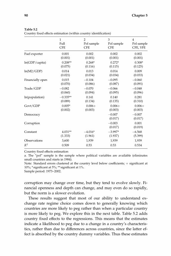
corruption may change over time, but they tend to evolve slowly. Fi-
nancial openness and depth can change, and may even do so rapidly,
but the norm is a slower evolution.
These results suggest that most of our ability to understand ex-
change rate regime choice comes down to generally knowing which
countries are more likely to peg rather than when a particular country
is more likely to peg. We explore this in the next table. Table 5.2 adds
country fixed effects to the regressions. This means that the estimates
indicate a likelihood to peg due to a change in a country’s characteris-
tics, rather than due to differences across countries, since the latter ef-
fect is absorbed by the country dummy variables. Thus these estimates
Table 5.2
Country fixed effects estimation (within country identification)
1FullCFE
2Pol sampleCFE
3Pol sampleCFE
4Pol sampleCFE, YFE
Fuel exporter 0.001 0.002 0.002 0.002(0.001) (0.001) (0.001) (0.001)
ln(GDP/capita) 0.208** 0.268* 0.272* 0.308*(0.075) (0.116) (0.115) (0.125)
ln(M2/GDP) 0.014 0.013 0.014 0.009(0.021) (0.034) (0.034) (0.033)
Financially open 0.015 �0.104 �0.095 �0.060(0.070) (0.086) (0.087) (0.091)
Trade/GDP �0.082 �0.070 �0.066 �0.048(0.060) (0.094) (0.095) (0.096)
ln(population) �0.335** 0.141 0.140 0.281(0.089) (0.134) (0.135) (0.310)
Govt/GDP 0.005* 0.006þ 0.006þ 0.006þ(0.002) (0.003) (0.003) (0.003)
Democracy �0.007 �0.007(0.017) (0.017)
Corruption �0.003 0.001(0.017) (0.019)
Constant 4.031** �4.016* �3.997* �6.568(1.333) (1.961) (1.937) (5.399)
Observations 3,600 1,939 1,939 1,939
R2 0.509 0.53 0.53 0.534
Country fixed effects estimationa. The ‘‘pol’’ sample is the sample where political variables are available (eliminatessmall countries and starts in 1984).Note: Standard errors clustered at the country level below coefficients; þ significant at10%; *significant at 5%; ** significant at 1%.Sample period: 1973–2002.
90 Chapter 5

cannot indicate the effect of unvarying country-specific variables like
distance to the base, sharing a border with the base, or being land-
locked. The remaining variables tend not to enter the regression signif-
icantly. Coefficients on oil revenues, financial openness, financial
depth, and political variables are not significant. There is a weak ten-
dency for countries to peg more often with a higher government share
of GDP and income per capita.
This point is important for the interpretation of results presented in
later chapters. The choice to peg is largely related to variables that
only change slowly, if at all.24 This diminishes concerns of endogene-
ity, whereby variables of interest, like inflation or economic growth,
are both determined by the peg and determine the likelihood to peg.
Rather, controlling for the level of development, political variables,
and the relationship with the base country—or simply using country
or country-pair fixed effects—seems to address adequately concerns
with endogeneity.
This result implies that the true dimension of interest is the cross sec-
tion, not the time series. A full panel may therefore present unwar-
ranted significance levels, even when adjusting the standard errors by
clustering. For this reason we also examine cross-sectional results with
specifications that are similar to those in table 5.1. We find almost
identical results as those found in that table, bolstering our contention
that the cross section is sufficient for understanding the choice of
the exchange rate regime (results not shown due to similarity with
table 5.1).
Our last three tables examine some of the insights presented in chap-
ter 4. First, we have noted that some countries peg for long periods of
time, but many pegs are short lived and countries flip back and forth.
Thus we will try to see if the determinants of being in a ‘‘long peg’’
look any different than that of being in a peg in general. As in chapter
4 we define a long peg as one that lasts at least five years. This does not
mean that an observation is coded as a long peg only after it has lasted
five years. The idea is that any pegged observation that is part of a peg
spell that lasts for at least five years is considered a long peg and
pegged observations that are part of a spell that breaks before five
years are considered a short peg. Likewise any float observation that is
part of a float spell that lasts at least five years is considered a long
float, and any observation that is a float that does not last that long is
a short float.25 We also merge the short pegs and short floats to create
a ‘‘short spell.’’ Thus countries that flip frequently are continually
marked as being in a short spell.
Empirics of Exchange Rate Regime Choice 91

We take the same set of covariates to see if there are different deter-
minants of being in a long peg, a short peg, or a short spell. The first
question, addressed in table 5.3, is to see if long pegs are driven by a
different set of economic variables than short pegs. The next question,
addressed in tables 5.4 and 5.5, asks if there is something different
about the countries that flip across exchange rate regimes.
Comparing the first column of table 5.3 to the first column of table
5.1, we see almost no difference between the determinants of long pegs
and the determinants of all pegs.26 This also generally holds when
including political variables, as shown by comparing columns 2 and 3
in these two tables (in each, the second column limits the sample to
observations for which political variables are available and the third
column augments the regression specification in the first column with
the democracy and corruption indicators). The only difference in the
determinant of long pegs versus all pegs is that the former are more
likely to arise in the presence of an open financial market.
The determinants of short pegs are investigated in the next three col-
umns of table 5.3, which compare short pegs to floats. The results in
these columns show that there is no tendency for short pegs to be con-
tiguous with the base, nor to have been a former colony. Also, coun-
tries in a short peg are no more likely to be oil exporters nor are they
any more likely to be democracies. This distinguishes these results
from those for long pegs. The only common significant determinant of
short pegs and long pegs relative to floats is that both are slightly more
likely to be found when financial depth is greater. There is a marked
difference in the overall goodness of fit of the short peg and long peg
regressions. The R2 statistics are between 0.20 and 0.30 in the long
peg regressions, but are basically zero in the short peg regressions.
The overall message, then, is that none of the variables that success-
fully explain why a country pegs in general can tell us why a country
engages in a short peg.
Table 5.4 considers a different question inspired by chapter 4; is there
something different about countries that flip? The dependent variable
is a dummy for being in a ‘‘short spell,’’ which is defined as either a
short peg or short float. Countries that are flippers, that is, that have
short spells, are less likely to have been a colony than countries that
peg or float, and they are less likely to be far from the base. These
results are logical in that short-spell countries are more apt to be close
to the base country than long-term floaters, and less likely to have
been colonies of the base country than long-term peggers. The results
92 Chapter 5
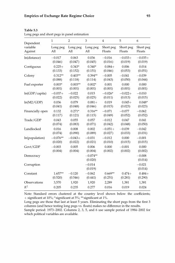
Table 5.3
Long pegs and short pegs in panel estimation
1 2 3 4 5 6Dependentvariable Long peg Long peg Long peg Short peg Short peg Short pegAgainst All All All Floats Floats Floats
ln(distance) �0.017 0.063 0.036 �0.016 �0.033þ �0.035þ(0.046) (0.047) (0.045) (0.016) (0.019) (0.019)
Contiguous 0.225þ 0.343* 0.340* 0.084þ 0.006 0.014(0.133) (0.152) (0.151) (0.046) (0.053) (0.051)
Colony 0.312** 0.403** 0.394** �0.005 �0.041 �0.039(0.088) (0.118) (0.114) (0.043) (0.050) (0.044)
Fuel exporter 0.003* 0.003** 0.002* 0.001 0.000 0.000(0.001) (0.001) (0.001) (0.001) (0.001) (0.001)
ln(GDP/capita) �0.037þ �0.022 0.015 �0.026* �0.022þ �0.010(0.022) (0.025) (0.025) (0.011) (0.013) (0.015)
ln(M2/GDP) 0.036 0.079 0.081þ 0.019 0.045þ 0.048*(0.041) (0.048) (0.046) (0.015) (0.023) (0.023)
Financially open 0.132 0.271* 0.316** �0.071 �0.077 �0.062(0.117) (0.121) (0.115) (0.049) (0.052) (0.052)
Trade/GDP 0.043 0.055 0.057 �0.012 0.047 0.041(0.074) (0.083) (0.071) (0.042) (0.048) (0.050)
Landlocked 0.016 0.008 0.002 �0.051þ �0.039 �0.042(0.074) (0.090) (0.089) (0.027) (0.033) (0.031)
ln(population) �0.076** �0.043þ �0.031 �0.012 0.000 �0.001(0.020) (0.022) (0.021) (0.010) (0.015) (0.015)
Govt/GDP �0.003 0.005 0.006 0.000 �0.001 0.000(0.004) (0.004) (0.004) (0.002) (0.002) (0.002)
Democracy �0.074** �0.008(0.020) (0.014)
Corruption �0.014 �0.021(0.019) (0.014)
Constant 1.657** �0.120 �0.062 0.669** 0.474þ 0.484þ(0.520) (0.546) (0.441) (0.251) (0.281) (0.290)
Observations 3,570 1,920 1,920 2,289 1,381 1,381
R2 0.205 0.235 0.277 0.016 0.019 0.024
Note: Standard errors clustered at the country level shown below the coefficients;þ significant at 10%; * significant at 5%; **significant at 1%.Long pegs are those that last at least 5 years. Eliminating the short pegs from the first 3columns (and hence testing long pegs vs. floats) makes no difference in the results.Sample period: 1973–2002. Columns 2, 3, 5, and 6 use sample period of 1984–2002 forwhich political variables are available.
Empirics of Exchange Rate Regime Choice 93

Table 5.4
Determinants of short spells
Dependent variable1Short spell
2Short spell
3Short spell
ln(distance) �0.040 �0.067* �0.070*(0.027) (0.028) (0.030)
Contiguous �0.010 �0.061 �0.058(0.080) (0.093) (0.092)
Colony �0.119* �0.142* �0.142*(0.047) (0.059) (0.058)
Fuel exporter 0.000 0.000 0.000(0.001) (0.001) (0.001)
ln(GDP/capita) �0.024 �0.030 �0.025(0.015) (0.022) (0.023)
ln(M2/GDP) 0.025 0.063þ 0.064þ(0.024) (0.036) (0.036)
Financially open �0.146* �0.234* �0.239*(0.070) (0.094) (0.096)
Trade/GDP �0.003 0.006 0.003(0.049) (0.062) (0.061)
Landlocked �0.042 �0.065 �0.064(0.044) (0.059) (0.058)
ln(population) 0.019 0.006 0.005(0.013) (0.022) (0.022)
Govt/GDP 0.002 �0.002 �0.002(0.003) (0.004) (0.003)
Democracy 0.009(0.016)
Corruption �0.021(0.019)
Constant 0.445 0.900þ 0.927þ(0.353) (0.480) (0.484)
Observations 3,570 1,920 1,920
R2 0.028 0.047 0.050
Note: Standard errors are clustered at the country level and are shown below the coeffi-cients; þ significant at 10%; * significant at 5%; **significant at 1%.The dependant variable is being in a short spell, either a short lived peg or float.Sample period: 1973–2002. Columns 2 and 3 use sample period of 1984–2002 for whichpolitical variables are available.
94 Chapter 5
in this table also show that flippers are more likely to have closed fi-
nancial markets than other countries.
Table 5.5 lets us more carefully isolate characteristics of countries
that flip a great deal as opposed to looking at all observations where a
country is in a short spell. The estimates in this table are based on a
data set of country means, using the sample that includes political vari-
ables. Thus there are 120 observations, representing the average values
for countries from 1984 to 2002, with one observation per country.
We group countries into three types: long peggers, long floaters, and
flippers. Long floaters are in a long float for at least ten years, long peg-
gers are in a long peg for at least ten years, and flippers fall into neither
of these categories.27 The results in column 1 show long peggers are
apt to be contiguous to the base and to have been a colony, but they
are less likely to be democratic. Fuel-exporting status does not show
up as a significant variable in this specification, and while there is a
tendency toward financial openness, its statistical significance is weak.
When compared to all countries, long floaters are less likely to have
been colonies, but nothing else is statistically significant. Similarly few
things mark flipping countries when they are compared to both long
pegs and long floats (column 4). They are less likely to be financially
open and more likely to have financial depth, but nothing else stands
out.
In summary, some variables that are consistent with basic theory
about exchange rate regime choice can tell us which countries are
likely to engage in long pegs. However, there is little that can contrib-
ute to our understanding of when a country pegs rather than floats,
nor is there a set of variables which significantly predict which coun-
tries are likely to flip back and forth across pegging and floating as op-
posed to staying in a long-term float. Crisis models, and the level of
the exchange rate, can help predict the timing of the end of a peg, but
not the duration of a float nor why some countries float and others
flip. Further, once the very small, very poor, long-term peggers are
dropped from the sample, some fairly basic, time-invariant variables
(proximity to the base and colonial relationship) seem to be dominant
rather than aspects about a country’s economy (e.g., GDP per capita
and usually not financial depth or population). Thus some fairly basic
controls concerning the relationship to the base (and certainly country
fixed effects) may be able to offset many of the concerns related to
endogeneity that one may have about the choice to peg when studying
the effects of pegging.
Empirics of Exchange Rate Regime Choice 95

Table 5.5
Regression of country types on country characteristics
1Long peggera
2Long floaterb
3Flipperc
ln(distance) 0.026 0.046 �0.066(0.054) (0.070) (0.055)
Contiguous 0.327þ �0.179 �0.112(0.175) (0.209) (0.199)
Colony 0.492** �0.370** �0.098(0.131) (0.132) (0.091)
Fuel exporter 0.001 0.000 �0.001(0.001) (0.002) (0.001)
ln(GDP/capita) 0.046 �0.076 0.018(0.042) (0.050) (0.038)
ln(M2/GDP) 0.058 �0.121 0.112þ(0.086) (0.099) (0.065)
Financially open 0.509þ 0.019 �0.499þ(0.276) (0.344) (0.279)
Trade/GDP 0.026 �0.142 0.039(0.135) (0.138) (0.116)
Landlocked �0.033 0.043 �0.063(0.108) (0.127) (0.078)
ln(population) �0.048 0.012 0.027(0.031) (0.041) (0.039)
Govt/GDP 0.009 �0.004 �0.005(0.007) (0.008) (0.006)
Democracy �0.089* 0.060 0.019(0.042) (0.055) (0.038)
Corruption �0.046 0.098 �0.039(0.045) (0.061) (0.049)
Constant 0.173 0.655 0.227(0.641) (0.910) (0.763)
Observations 123 123 123
R2 0.337 0.203 0.114
Note: Robust standard errors shown below the coefficients; þ significant at 10%; * sig-nificant at 5%; ** significant at 1%.a. Long pegger is in a long peg at least 50% of the time.b. Long floater is in a long float at least 50% of the time.c. Flipper is neither (spends most of their time in a short spell).Regressions run on country means over the 1984–2002 sample where political variablesare available.
96 Chapter 5

5.4 Conclusion
This chapter differs from others in the book in that it considers the
determinants of the exchange rate regime rather than its consequences
or its attributes. A central result is that country-specific variables that
are largely time invariant do a better job of explaining exchange rate
regime choice than time-varying variables.
There is an important implication of the result that constant country
characteristics are a central determinant of exchange rate regime choice
for the analysis presented in later chapters. In those chapters, we exam-
ine the consequences of exchange rate regime choice for international
trade, growth, and macroeconomic stability. The results presented in
this chapter suggest that endogeneity is not likely to be a problem for
those regressions as long as proper controls are considered, a result
confirmed in those chapters.
Empirics of Exchange Rate Regime Choice 97


III Exchange Rate Consequences of Exchange RateRegimes

6 Exchange Rate Regimes and Bilateral ExchangeRates
Let deeds match words.
—Titus Maccius Plautus, ancient playwright
Saying doesn’t make it so. Or, in the case of exchange rate regimes, a
government that declares that it has a floating exchange rate might not
in fact allow its currency to freely fluctuate. For the exchange rate re-
gime to matter to economic outcomes, it seems a prerequisite that the
regime makes a difference in the behavior of the exchange rate. These
next two chapters will consider what we might call the exchange rate
effect of fixed exchange rates.
The mere classification of annual observations into those categorized
as pegs and those categorized as floats (or, more accurately, nonpegs)
would not matter if the governments shied away from volatility and
truly limited exchange rate flexibility when countries do not peg. As
discussed in chapter 4, Calvo and Reinhart (2002) argue that govern-
ments that declare they float exhibit a ‘‘fear of floating,’’ that is, an
aversion to allowing their currencies’ values to be determined by the
foreign exchange market. But if this is the case, then the distinction be-
tween fixed and floating exchange rate regimes discussed in part II of
this book might have little economic consequence. We show in this
chapter, however, that while numerous declared floats are actually
pegged or heavily managed floats, countries that do float show a dis-
tinctly different pattern of exchange rate behavior than those that peg.1
That is, we demonstrate in this chapter that after properly accounting
for which countries peg and which float, there are clear differences in
exchange rate volatility between these two categories.
The qualitative result that one can associate lower bilateral vola-
tility with de facto pegs is not striking, and may even be viewed as
tautological, but the interesting question is the quantitative implica-
tions of pegging. Currency pegs, by definition, exhibit more bilateral
exchange rate stability than floating exchange rates—if the volatility of
floats were identical to that of pegs, they would all be considered
pegs—but how much more? The ‘‘fear of floating’’ result suggests that
this difference is not large. We demonstrate, however, that the magni-
tude of bilateral exchange rate volatility between a country that has a
pegged rate and its base country is distinct from bilateral volatility
when a country does not peg. The focus of the chapter is to show that
the size of the difference in volatility is meaningful, and that the bulk
of countries that are coded as floats look more like a classic float rather
than just a loose peg. These results are obtained even when controlling
for country and year fixed effects, and for inflation behavior and capi-
tal controls.
Another important point established in this chapter concerns the
continuing effects of a peg. Many economic decisions regarding ex-
change rates incorporate forward-looking behavior; for example, con-
tracts for international trade are signed six months to two years before
actual delivery and payment takes place. Thus today’s peg must tell us
something about the future to affect actions initially undertaken today
that have implications for future transactions. We find that differences
in volatility between pegged and floating exchange rate arrangements
persist into the future. A peg in one year predicts lower volatility for a
number of subsequent years.
The skepticism of the fear of floating school runs against the well-
known results of Mussa (1986) which show that bilateral real exchange
rate volatility was distinctly different across exchange rate regimes.
This result stems primarily from differences in bilateral nominal ex-
change rate volatility. Mussa’s results were revisited and confirmed in
numerous studies, such as Baxter and Stockman (1989) and Liang
(1998).2 We focus in this chapter on bilateral nominal volatility as it di-
rectly addresses the question of whether pegs matter and because the
real exchange rate result has already received much attention.
Thus, before we move on to consider the effects of exchange rate
regimes in part IV, we establish an economically relevant distinction
between the exchange rate behavior of fixed and floating exchange
rate regimes. In this chapter we focus on the bilateral exchange rate be-
tween a country and its natural base. In the next chapter we consider a
similar set of questions for multilateral exchange rates.
102 Chapter 6

6.1 Indisputable and Disputable Floats
Some countries indisputably allow their currencies to float. Calvo and
Reinhart (2002) often cite the benchmark of Australia and Japan as
examples of idealized floats. An examination of the behavior of their
dollar exchange rates supports this judgment. For example, the Japa-
nese yen has moved considerably over the past three decades, appreci-
ating from ¥360/US$1 in the early 1970s to a rate as strong as ¥80/
US$1 in 1995, back up to over ¥140/US$1 in 1998, and dipping below
¥100/US$1 a decade later. This might well be taken as prima facie evi-
dence that Japan has a floating exchange rate regime, even though the
Bank of Japan has used its foreign exchange reserves to intervene in
the market. Similarly the Australian dollar began the modern era at
$0.71/US$1 in March 1973, depreciated to $1.63/US$1 about a dozen
years later, and further to almost $2.00/US$1 at the beginning of this
century, before strengthening to within four cents of parity in 2008.
But how typical are these experiences? Calvo and Reinhart argue
that the dollar exchange rates of the yen and the Australian dollar
(along with some other currencies, like the deutsche mark in the pre-
euro period) behave differently than the bulk of other flexible exchange
rates, and that ‘‘fear of floating’’ is pervasive. One way to judge this ar-
gument is to compare the historical volatility of the dollar exchange
rates of the yen, the Australian dollar, and the deutsche mark to those
of other floating currencies. This requires a calculation of volatility and
also a classification that gives us a set of country–year observations for
which the exchange rate is judged to be floating. We calculate volatility
as the standard deviation of the monthly percentage change in the ex-
change rate, which is the formula typically used (e.g., see Lane and
Devereux 2003; Rose 2000).3 We use the Klein–Shambaugh classifica-
tion scheme described in chapter 4 to obtain a set of country–year
observations that are classified as floating from the full sample of 125
countries in the 1973 to 2004 period.4
This exercise shows that the average exchange rate volatility of the
currencies of Australia, Japan, and Germany are not outliers in this set
of floating exchange rate observations. In particular, the average vola-
tilities of the bilateral dollar exchange rates of these countries fall with-
in the 50th and 60th percentiles of the set of country–year volatility
statistics for the set of floating observations. If we drop the first year of
float spells, observations that are typically more volatile than other
Bilateral Exchange Rates 103
years in spells, the average volatilities of these three countries are with-
in the 60th and 70th percentiles, a higher level, to be sure, but far from
atypical of the set as a whole.
6.2 Volatility in Floats and Pegs
Placing the volatility of the bilateral US dollar exchange rates of Aus-
tralia, Germany, and Japan in context shows that these acknowledged
paradigms of floating actually exhibit fairly typical behavior for the set
of floating observations as a whole. In this section we consider the vol-
atility of the entire set of floating observations as compared to the en-
tire set of pegged observations. It will not be surprising, of course, that
we find that the volatility of the floating observations is greater than
that of the pegged observations; the question is the extent to which the
former exceeds the latter, and whether there is a meaningful distinction
between the two groups.
We begin by considering the extent of the overlap in measured vola-
tility between the set of float observations and the set of peg observa-
tions where, once again, the Klein–Shambaugh classification system is
used to distinguish pegs from floats. We sort the set of annual observa-
tions by exchange rate volatility. We then divide these observations
into quintiles, and determine the number of peg observations in each
of the five quintiles.5
If volatility between peg observations and float observations were
roughly equal, we would expect to find that each quintile would have
about half peg observations and half float observations, since the sam-
ple is roughly divided evenly between pegs and floats. If pegs and
floats are truly distinct, we expect to see all the pegs in low volatility
quintiles and all the floats in high volatility quintiles. Figure 6.1 shows
the percentage of observations pegged in each volatility quintile. The
lowest quintile of bilateral volatility among country–year observations
consists exclusively of pegs. The second quintile includes 87 percent
annual peg observations. The third quintile is a middle ground and is
more evenly split between peg and float observations.6 But the fourth
and fifth quintiles are almost exclusively the province of floating ob-
servations. Thus pegs and floats demonstrate distinctly different
volatility.7
While these results show that pegs and floats occupy different parts
of the volatility distribution, the question remains about the magnitude
of the difference in volatility across these regimes.8 We examine this by
104 Chapter 6
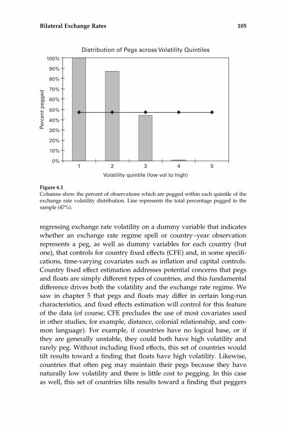
regressing exchange rate volatility on a dummy variable that indicates
whether an exchange rate regime spell or country–year observation
represents a peg, as well as dummy variables for each country (but
one), that controls for country fixed effects (CFE) and, in some specifi-
cations, time-varying covariates such as inflation and capital controls.
Country fixed effect estimation addresses potential concerns that pegs
and floats are simply different types of countries, and this fundamental
difference drives both the volatility and the exchange rate regime. We
saw in chapter 5 that pegs and floats may differ in certain long-run
characteristics, and fixed effects estimation will control for this feature
of the data (of course, CFE precludes the use of most covariates used
in other studies, for example, distance, colonial relationship, and com-
mon language). For example, if countries have no logical base, or if
they are generally unstable, they could both have high volatility and
rarely peg. Without including fixed effects, this set of countries would
tilt results toward a finding that floats have high volatility. Likewise,
countries that often peg may maintain their pegs because they have
naturally low volatility and there is little cost to pegging. In this case
as well, this set of countries tilts results toward a finding that peggers
Figure 6.1
Columns show the percent of observations which are pegged within each quintile of theexchange rate volatility distribution. Line represents the total percentage pegged in thesample (47%).
Bilateral Exchange Rates 105
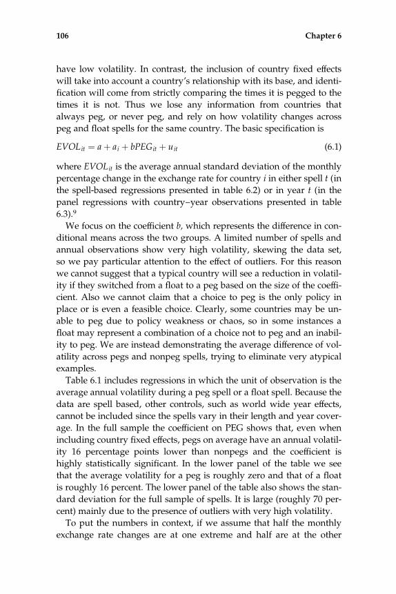
have low volatility. In contrast, the inclusion of country fixed effects
will take into account a country’s relationship with its base, and identi-
fication will come from strictly comparing the times it is pegged to the
times it is not. Thus we lose any information from countries that
always peg, or never peg, and rely on how volatility changes across
peg and float spells for the same country. The basic specification is
EVOLit ¼ aþ ai þ bPEGit þ uit (6.1)
where EVOLit is the average annual standard deviation of the monthly
percentage change in the exchange rate for country i in either spell t (in
the spell-based regressions presented in table 6.2) or in year t (in the
panel regressions with country–year observations presented in table
6.3).9
We focus on the coefficient b, which represents the difference in con-
ditional means across the two groups. A limited number of spells and
annual observations show very high volatility, skewing the data set,
so we pay particular attention to the effect of outliers. For this reason
we cannot suggest that a typical country will see a reduction in volatil-
ity if they switched from a float to a peg based on the size of the coeffi-
cient. Also we cannot claim that a choice to peg is the only policy in
place or is even a feasible choice. Clearly, some countries may be un-
able to peg due to policy weakness or chaos, so in some instances a
float may represent a combination of a choice not to peg and an inabil-
ity to peg. We are instead demonstrating the average difference of vol-
atility across pegs and nonpeg spells, trying to eliminate very atypical
examples.
Table 6.1 includes regressions in which the unit of observation is the
average annual volatility during a peg spell or a float spell. Because the
data are spell based, other controls, such as world wide year effects,
cannot be included since the spells vary in their length and year cover-
age. In the full sample the coefficient on PEG shows that, even when
including country fixed effects, pegs on average have an annual volatil-
ity 16 percentage points lower than nonpegs and the coefficient is
highly statistically significant. In the lower panel of the table we see
that the average volatility for a peg is roughly zero and that of a float
is roughly 16 percent. The lower panel of the table also shows the stan-
dard deviation for the full sample of spells. It is large (roughly 70 per-
cent) mainly due to the presence of outliers with very high volatility.
To put the numbers in context, if we assume that half the monthly
exchange rate changes are at one extreme and half are at the other
106 Chapter 6

extreme, the estimated intercept and slope coefficients suggest that
monthly changes in the �1 to 1 percent range for pegged observations
and the large range of about �16 to 16 percent for floating exchange
rates. The ranges consistent with these estimated coefficients could in
fact be larger if some monthly changes are not at the extreme values.10
A sample without outliers gives us a better picture of a typical float.
We use a sample that excludes spells that represent the top 1 percentile
of volatility. As seen in column 2 of table 6.1, the standard deviation of
this sample drops considerably, even though we have only eliminated
1 percent of the observations. In this case the coefficient on PEG is less
than half as big as in the full sample regression (though it remains sta-
tistically significant) and its (absolute) value of 0.07 is now nearly equal
to the standard deviation of the dependent variable. That is, once out-
liers are removed, pegs have a roughly one standard deviation lower
volatility than floats when we have controlled for country fixed effects.
Also, once outliers are removed, the R2 jumps up to 0.31 with only the
dummy for pegging and country fixed effects in the regression. This is
notable given that the peg variable, by definition, only distinguishes
between pegs and floats and cannot help explain differences within
the floating group. The bottom panel of the table shows that pegs have
Table 6.1
Exchange rate volatility in spells
Sample1Full
2Drop 1%
Peg �0.158** �0.068**(0.051) (0.008)
Constant 0.161** 0.071**(0.026) (0.004)
Observations 792 785
R2 0.170 0.310
Sample standard deviation 0.689 0.086
Peg mean 0.004 0.004
Peg med 0.003 0.003
Nonpeg mean 0.161 0.069
Nonpeg med 0.025 0.024
Note: Standard errors are clustered at the country level; country fixed effects are in-cluded. Column labeled ‘‘Drop 1%’’ drops the 1% largest volatility observations to reducethe impact of outliers. * represents a statistically significant difference from zero at the95% confidence level, **at the 99% level. Sample: spells covering 125 countries from1973–2004.
Bilateral Exchange Rates 107

roughly zero volatility and nonpegs (excluding the top 1 percentile
group) have volatility close to 7 percent. Many floats with an annual
volatility of 7 percent typically show a range in the monthly change in
the level of the exchange rate of �3 percent to 5 percent, with one
month in the mid 20 percent range (e.g., Spain 1977, New Zealand
1984, and Fiji 1998).11 The message from these results is that, while
there may be fear of floating behavior, the typical floating country has
considerably more exchange rate volatility than a peg.12
The estimates in table 6.2 are based on regressions in which the unit
of observation is a country–year data point rather than a peg spell or a
float spell. These data allow us to include year effects (to take into ac-
count that some years may have seen broad volatility across the globe)
and annual covariates that align directly to our data. This analysis also
allows for estimating whether the first year of a floating spell is
marked by an unusually high level of volatility; thus the estimates on
the peg dummy in specifications that include a first-year-of-float
dummy are interpreted as the effect of a peg as compared to a second
or subsequent year of a float. As in table 6.1 we seek to eliminate the
effect of a few extreme outlier cases, so our estimates in table 6.2 are
based on samples that drop the 1 percent most volatile country–year
observations.13 Once again, we include country fixed effects. Com-
bined with year fixed effects, which control for differences in world
volatility from year to year, CFE allow us to isolate the differences in
volatility across pegs and nonpegs controlling for differences in coun-
try behavior.
The estimates in the first column of table 6.2 indicate that annual vol-
atility is 5 percentage points lower for peg country–year observations
than for float country–year observations. The estimate in the second
column shows that annual volatility for pegs is 4.2 percentage points
lower for pegs than for non-first-year floats, and volatility is 2.4 per-
centage points higher during the first year of a float than during sub-
sequent years. The median for bilateral float volatility is close to that
of Japan in 1984 (2 percent volatility) when its monthly percentage
changes ranged from �4 percent to 3 percent and the yen/dollar rate,
beginning the year at ¥235/US$1, went as low (in the end-of-month
data) as ¥220/US$1 and as high as ¥250/US$1. The mean for non-first-
year float floats was 3.8 percent, which is similar to Germany in 1981
when monthly changes ranged from 8 percent to �4 percent and the
DM ranged from DM2.1/US$1 to DM2.46/US$1. These were not crisis-
driven years, but represent the average volatility of floats, considerably
108 Chapter 6

different than the pegged countries staying in the 2 percentage bands
where behavior is usually close to 1 percent up or down a month. By
definition, the maximum annual range of the exchange rate for pegs
wase2 percent, the median was less thane0.5 percent. For floats, the
average range was e12 percent (median e6 percent). For example, a
year when the yen/dollar exchange rate ranged from 120 to 135 would
be at the median range and between 120 and 150 would be the average
range. It is important to note that these ‘‘classic’’ floats, as mentioned
above, are near the middle of the distribution. They are not unusual
floats in terms of the magnitude of volatility. They are fairly typical
descriptions of the experiences of floats.
Table 6.2 also includes estimates in which we control for other
aspects of a country’s economy. The third column shows that inflation
is positively and significantly correlated with volatility, and volatility
is also higher in the presence of capital controls (although not signifi-
cantly so). But, even with these covariates in the regression, a peg is
Table 6.2
Exchange rate volatility in annual panel data
1 2 3
Peg �0.049** �0.042** �0.031**(0.005) (0.004) (0.003)
First-year float 0.024** 0.033**(0.006) (0.007)
Inflation 0.074**(0.010)
Capital controls 0.006(0.004)
Constant 0.035** 0.032** 0.014**(0.002) (0.002) (0.005)
Observations 3,816 3,816 3,546
R2 0.25 0.26 0.37
Sample standard deviation 0.056 0.056 0.055
Peg mean 0.002 0.002 0.002
Peg median 0 0 0
Nonpeg mean 0.042 0.042 0.041
Nonpeg median 0.02 0.02 0.02
Note: Standard errors are clustered at the country level and are shown below the coeffi-cients. Country fixed effects and year fixed effects are included in all specifications. Thesample drops the 1% largest volatility observations to reduce the impact of outliers,and column 3 drops the 1% largest outcomes of inflation. * represents statistically signifi-cantly different from zero at the 95% confidence level, **at the 99% level. Sample: 125countries from 1973–2004.
Bilateral Exchange Rates 109

substantially more stable than a nonpeg with relatively little change to
the magnitude of the coefficient on the peg dummy. Results hold
across industrial countries and nonindustrial countries with means
and coefficients smaller for industrial countries and first-year floats not
associated with higher volatility for rich countries.
6.3 Persistent Effects of Pegging
Section 6.2 demonstrates that the exchange rate matters for current
year exchange rate volatility. However, for the exchange rate regime
to matter to a number of outcomes that we explore later in the book, it
is important to discern whether a peg today suggests lower volatility
in future years.
We investigate this question by running a series of regressions of ex-
change rate volatility on peg status (with year and country fixed effects
included) that are similar to those in column 1 of table 6.2 but for suc-
cessive lags of the peg dummy variable, rather than its contemporane-
ous value. That is, we first test the impact of being pegged today on
today’s volatility, and then separately test the impact of being pegged
today on volatility next year, and in subsequent years, regardless of
what happens to the exchange rate regime in those future years.
The estimates from this analysis are presented in figure 6.2. The
numbers along the horizontal axis in these figures represents the num-
ber of years that the peg variable is lagged in a regression of country–
year volatility on a peg dummy. Thus, the point associated with the
zero value in each of these figures represents the current year effect of
a peg on exchange rate volatility, that is, the coefficient reported in col-
umn 1 of table 6.2. The associated horizontal lines around these points
represent a confidence interval equal to two times the standard error.14
The other points and lines represent point estimates and standard
errors from the regressions using 1, 2, 3, 4, and 5 year lags of the peg
variable. The regressions are estimated using the lagged peg dummy
variable regardless of the subsequent history of the peg spell.
Figure 6.2 shows that the effect of a peg extends, in a significant way,
up to two years in the future. Both the one- and two-year lags of pegs
are associated with significantly lower bilateral volatility. Earlier lags
than these, however, have relatively small impacts on volatility.15
Thus a peg today suggests lower volatility today, next year, and the
year after that, but this effect fades once one moves out beyond two
years.
110 Chapter 6

Given the results of chapter 4 that pegs often break, it is no surprise
that a peg today does not suggest lower volatility indefinitely. Yet we
also saw that pegs became more durable over time. First-year pegs
were the most fragile. Reestimating these results without the first year
of pegs (which eliminates one-year pegs) increases the persistent effect
of a peg on subsequent bilateral volatility for the one- and two-year
horizons, as the remaining pegs are more durable and more likely to
re-form if broken (these points are shown as squares on the figures),
but makes no difference after that.
These results are important in exploring how pegs could have an im-
pact on forward-looking economic behavior. A peg today does suggest
lower volatility in the future. These results suggest why, for example,
Klein and Shambaugh (2006) find an increase in bilateral trade from
pegging even when controlling for contemporaneous volatility, since a
peg today implies lower exchange rate volatility in the future.16
Figure 6.2
Bilateral volatility over time. Time 0 represents the contemporaneous coefficient of ex-change rate volatility on pegging, time 1 represents the coefficient on a lagged peg, andso on. Thus the point at time 2 represents the difference in volatility for a country thatwas pegged two years ago (whether it has remained pegged or not). Country- and year-fixed effects are included. The dark lines represent 2 times standard error bands aroundthe main point estimates, where standard errors are clustered on country. To ensure thatthe comparison is with nonpegged observations, new pegs that are not re-pegs areexcluded (see text). Squares represent the point estimate if the first year of pegging isexcluded.
Bilateral Exchange Rates 111

6.4 Exchange Rate Outcomes across Classifications
We also examine our volatility results across the different exchange
rate regime classifications that were discussed in chapter 3. For some
questions such an exercise could be considered merely a robustness
test—examining if the results are sensitive to the definition of a peg. In
this case, however, the results go beyond robustness to shed more light
on the variation of conceptions undergirding classifications schemes.
Table 6.3 demonstrates the broad similarity of the overall pattern
across schemes. Pegs tend to fill most of the lower volatility quintiles
and are found less frequently in the top two. The differences across the
columns are nevertheless informative. A source of the difference be-
tween the Klein–Shambaugh based results presented in sections 6.1
through 6.3 and those obtained when the peg dummy is defined using
the Shambaugh classification is that the latter allows a peg to continue
through a one-time devaluation, and consequently more volatile ex-
change rate outcomes can be called pegs. Likewise pegs can last
through devaluations in the Reinhart–Rogoff classification, and for
this reason the Reinhart–Rogoff results look similar to the Shambaugh
results with regards to the percentage of high volatility outcomes that
are pegs (11 percent). Also, the Reinhart–Rogoff classification does not
count all stable official rates as pegs (due to the use of secondary mar-
ket rates), and thus many of the most stable outcomes are nonpegs (100
percent � 71 percent ¼ 29 percent). Reinhart–Rogoff is the only de facto
classification that has many stable observations labeled as floats. There
are also instances of low-volatility observations labeled as de jure non-
Table 6.3
Percentage pegged by exchange rate volatility quintile
KSpeg JSpeg RRpeg DJpeg LYSpeg
1 100% 99% 71% 89% 99%
2 87% 83% 58% 66% 93%
3 44% 31% 16% 21% 41%
4 1% 1% 7% 9% 39%
5 0% 11% 11% 20% 21%
Total 47% 45% 33% 41% 58%
Note: As in figure 6.1, the table shows the percentages of annual observations that arepegged in each quintile of exchange rate volatility. The bottom row shows the total shareof pegs in the entire sample for each classification. KS ¼ Klein–Shambaugh, JS ¼ Sham-baugh, RR ¼ Reinhart–Rogoff, DJ ¼ de jure, LYS ¼ Levy–Yeyati and Sturzenegger.
112 Chapter 6

pegs, as some countries that declare a float actually limit exchange rate
volatility tightly. In addition a fifth of the de jure pegs are highly vola-
tile since some countries declare pegs that do not hold. The LYS classi-
fication scheme also has a large number of volatile pegs; 21 percent of
the high-volatility outcomes are labeled pegs, a higher percentage basis
then even the de jure classification. These high-volatility pegs are not
discrete devaluations but simply moderate to high volatility outcomes
that are labeled pegs in their cluster analysis technique.
We also examine regressions such as those in table 6.2 for the differ-
ent classifications. The most notable difference on the exchange rate
effects of pegging across classifications is that with the de jure classifica-
tion the coefficient on PEG variable is not significantly different from
zero. This result, and others using the Reinhart–Rogoff, Shambaugh,
and LYS classifications, are presented in table 6.4. This table includes
specifications matching those in column 2 of table 6.2 to show how the
effect of a peg on exchange rate volatility depends on the classification
employed. The results in columns 1 and 2 show that the Shambaugh
and Reinhart–Rogoff classification schemes, which allow peg spells to
continue through one-time devaluations, result in weaker results for
the coefficient on PEG than is the case with the Klein–Shambaugh clas-
sification scheme used in table 6.2 (the coefficient is �0.042 with Klein–
Shambaugh, but �0.025 with Shambaugh and �0.013 with Reinhart–
Rogoff). The result in column 3 shows that the misidentification of
Table 6.4
Exchange rate volatility in annual panel data across classifications
1 2 3 4
Classification JS RR DJ LYS
Peg �0.025** �0.013** �0.001 �0.033**(0.004) (0.004) (0.005) (0.004)
First-year float 0.027** 0.017 0.035** 0.034*(0.007) (0.012) (0.010) (0.007)
Constant 0.020** 0.025** 0.013** 0.031*(0.003) (0.005) (0.003) (0.003)
Observations 3,816 3,101 3,704 3,088
R2 0.18 0.16 0.15 0.31
Note: this table reproduces column 2 from table 6.2, for bilateral exchange rate volatility,across classifications. There are country and year fixed effects included, 1% outliers aredropped, and standard errors are clustered at the country level. The change in the num-ber of observations across columns is due to different availability of the classifications.* represents statistically significantly different from zero at the 95% confidence level, **atthe 99% level.
Bilateral Exchange Rates 113
regimes that occurs with de jure classifications results in insignificant
coefficients on PEG.17 The result in column 4 demonstrates that the co-
efficient on PEG is weaker when using the LYS classification than that
obtained with the Klein–Shambaugh classification (as in table 6.2)
since the LYS classification includes more volatile observations as
pegs. However, the results using LYS classification are stronger than
those with the Reinhart–Rogoff or Shambaugh classifications because
Levy-Yeyati and Sturzenegger do not classify cases with very large
devaluations as continuing pegs.
6.5 Volatility and the End of Exchange Rate Pegs
We consider one final question regarding volatility. Does a peg simply
bottle up volatility until a crash? If so, pegs only delay, not repress, ex-
change rate volatility. This was a key contention of Friedman (1953) in
part of his argument as to why floats would not be more volatile than
pegs. He argued that smoothly floating exchange rates would generate
less volatility than the large devaluations within adjustable peg
regimes.18 One might also worry that the longer a peg exists, the more
spectacular will be its collapse. To test this idea, we look at whether
high volatility is tied to the end of a peg regime in three different ways.
Panel A of table 6.5 divides the 37 top 1 percent volatility outcomes
and the 187 top 5 percent volatility outcomes according to whether the
preceding year was one in which the exchange rate was pegged or
whether it floated. There is nearly an even division between these cate-
gories, with slightly fewer high volatility observations following a peg
and slightly more following a float. The 37 top 1 percent volatility out-
comes are divided between 21 that followed a float year (which is 1.1
percent of the float observations) and 16 that followed a peg (which is
0.9 percent of the peg observations). Similarly 118 of the 187 top 5 per-
cent volatility observations followed a float (representing 5.9 percent of
the float observations) while the remaining 69 followed a peg (4.0 per-
cent of the peg observations). Thus an extremely high volatility out-
come is not significantly more likely to follow a peg than it is to follow
a year in which the exchange rate was not pegged.19
The statistics presented in panel B of table 6.5 allows us to consider
whether a year in a pegged regime of a particular length is followed
by a high-volatility year, regardless of whether these dates in the peg
spell actually represented the terminal year of the peg. There is a
slightly higher value for the percentage of extremely high (top 1 and
114 Chapter 6

top 5 percent) volatility observations that follow in the wake of a one-
year peg (1.5 and 4.6 percent respectively), but the differences are
not especially notable. Thus we see that at the start of a year, regard-
less of how long a peg has lasted, the odds of a spectacular collapse
are about the same (and again, as seen in panel A, are roughly the
same as for a floating observation).
A striking difference across the length of a peg does arise, however,
when we look at exchange rate pegs that break. This is shown in panel
C of table 6.5. The statistics in this part of the table show that 8.8 per-
cent of the years immediately following the breakup of a long (i.e.,
longer than five-year) peg are in the set of the top 1 percent volatility
observations, and more than half (54.4 percent) of these long peg col-
lapses are in the set of the top 5 percent volatility observations. The
comparable numbers for one-year pegs and for pegs that last between
two and five years are much smaller. Because long pegs are more likely
to survive, a randomly drawn long peg observation is no more likely
than any other to be followed by a high volatility outcome. But, once
a long peg does collapse, it is far more likely to collapse in a chaotic
fashion.
Table 6.5
Exchange rate regime status in year prior to high-volatility outcomes
Obser-vationsa
In top1%b Percent
In top5% Percent
Panel A
Full sample 3,738 37 1.0% 187 5.0%
Nonpeg in previous year 1,998 21 1.1% 118 5.9%
Peg 1,740 16 0.9% 69 4.0%
Panel B
Pegged in previous yearwith peg representing:
First year of pegging 388 6 1.5% 18 4.6%
2–5 years of pegging 575 5 0.9% 20 3.5%
>5 years of pegging 777 5 0.6% 31 4.0%
Panel C
Final year of peg 342 16 4.7% 69 20.2%
One-year peg spell 173 6 3.5% 18 10.4%
2–5-year peg spell 112 5 4.5% 20 17.9%
>5-year peg spell 57 5 8.8% 31 54.4%
a. Total number of observations following a given exchange rate regime status.b. Number of observations in the top 1% of the volatility distribution.
Bilateral Exchange Rates 115

Thus, the message from table 6.5 is that high volatility outcomes are
no more likely to follow a year in which a currency was pegged than a
year in which a currency floats. Also the number of years that a peg
has been ongoing is not especially informative for predicting whether,
in the next year, there will be an extremely high volatility outcome.
But if we know that a peg ends after a particular number of years, we
can predict that volatility is higher if the peg has lasted longer.20 The
distinction between the second and the third statements reflects the
fact that there is a decreasing hazard for pegs; the longer the peg lasts,
the less likely that it will break in a subsequent year, but if it does
break, it does so in a more spectacular fashion if it is older than if it is
younger.
6.6 Conclusion
As our discussion in chapter 3 makes clear, it is unquestionable that
many countries limit their exchange rate volatility, despite their claims
that they allow their currencies to float. But this leaves open the ques-
tion of how different actual pegs and floats are. We find that the mag-
nitude of the gap in volatility is substantial. The average or median
float does conform to our standard view of a float—one where the ex-
change rate can move a fair bit over the course of a year. Classic floats
such as the yen or Australian dollar are not atypical but stand in the
middle of our volatility distribution. A typical floating observation
simply has a considerable amount more volatility than a peg, even
when we control for country and year fixed effects and the first year of
floating. In addition, despite the fragility of pegs, enough pegs last (or
re-peg quickly) such that pegging today is a good predictor of low vol-
atility in the future, suggesting that we might expect pegs to have a
real effect on economic outcomes. Further, these pegs have not simply
bottled up volatility until a spectacular collapse since floating countries
also find themselves thrown into very high volatility outcomes at
roughly the same rate. The next chapter extends this analysis to con-
sider exchange rate indexes that look at the movement of the exchange
rate against some weighted average of currencies as opposed to strictly
the base currency.
116 Chapter 6
7 Exchange Rate Regimes and Multilateral ExchangeRates
You can only do one thing at a time.
—Maxwell Maltz, Pyscho-Cybernetics (1960)
An exchange rate is inherently bilateral. That is, one cannot speak pre-
cisely about the dollar depreciating or appreciating without specifying
the currency against which it moves. The dollar could be rising against
one currency and falling against another at the same time. This seem-
ingly simple observation is a crucial one for the economics of exchange
rate regimes in the modern era. It also distinguishes the modern era
from the gold standard or Bretton Woods periods when the use of a
common anchor by nearly all countries meant that pegs in those eras
would almost automatically be stabilizing the multilateral as well as
the bilateral exchange rate.
In the modern era, the general rule is that a country can only peg its
exchange rate against one particular currency or, in some cases (e.g.,
with the euro, post-1999), against the currency used by a set of coun-
tries. For example, in the 1990s Argentina pegged to the US dollar.
This stabilized its dollar exchange rate, but as the dollar appreciated
against European currencies in the latter part of that decade, so did the
Argentine peso.
Chapter 6 demonstrated that exchange rate pegs significantly reduce
bilateral exchange rate volatility, and that floats have considerably
more bilateral volatility than pegs. But a country with trade and invest-
ment across the globe will worry about many different exchange rates.
Since a country cannot stabilize its exchange rate against all countries,
just against one other currency, we are left wondering whether a bilat-
eral exchange rate peg stabilizes a broader measure of the value of a
currency.1
The need to summarize the value of a currency, rather than speak of
how the exchange rate has moved against each partner currency, leads
us to study an average value—or index value—of a currency. A multi-
lateral exchange rate index weights the value of a currency against all
partner currencies, typically using trade shares to weight the various
bilateral exchange rates. Thus, if half of US trade is with the euro area,
a quarter with Japan, a quarter with Canada, we would take the value
of the dollar against each currency and create an average using these
weights. Then we could track the weighted average value of the dollar.
These indexes are sometimes referred to as effective exchange rate
indexes.
The usefulness of an index goes beyond the ability to simply sum-
marize a currency’s standing. While some outcomes depend on the sta-
bility of a bilateral exchange rate with the base (e.g., trade with the
base or the stability of the nominal anchor), many others are probably
more dependent on the stability of a properly weighted index of the
exchange rate, for example, overall trade or import price stability. A
stable bilateral rate coupled with an unstable multilateral rate could be
associated with instability in the overall prices of imports and exports.
A fixed bilateral exchange rate could affect the multilateral index
through three routes. First, it can stabilize one part of the index, the
exchange rate against the base country. If the base country is a sub-
stantial part of the index, this may importantly contribute to the
stabilization of the index. Second, other countries may peg to the base
as well which would lead to even more stability in the index. This was
more important during the gold standard and the Bretton Woods eras
than during the modern era when there has been heterogeneity in both
base countries and exchange rate arrangements. Finally pegs may
avoid very high volatility outcomes, especially for emerging market
and developing countries, by providing a nominal anchor. This stabil-
izes that country’s currency to a wider set of industrial countries than
just its own base, since most volatility among the currencies of indus-
trial countries is relatively low compared to that of some emerging
market and developing countries.
This chapter shows how the exchange rate regime can, and does, af-
fect the overall exchange rate index. We will examine the nominal ef-
fective exchange rate, representing the relative price of monies across
countries, as well as the real effective exchange rate, representing the
relative price of goods and services across countries.
118 Chapter 7

7.1 Literature on Multilateral Volatility
The literature on the exchange rate effects of a fixed exchange rate has
tended to focus on the bilateral rates. As discussed in the previous
chapter, the work of Mussa (1986) and those that followed saw a con-
siderable effort to document the way the bilateral real exchange rate
varies across exchange rate regimes. The work on multilateral ex-
change rates is more limited. Klein and Shambaugh (2008) examine
this topic, and we return to empirical work based on those estimates
in section 7.2.
Some authors present limited discussions of multilateral volatility in
broader surveys of the impact of exchange rate regimes. Ghosh et al.
(2002) present averages of nominal and real multilateral volatility
across exchange rate regimes. They show that nominal volatility is
larger for floating countries than for countries that peg. The differences
across sets of countries, based on their exchange rate arrangements, are
less marked for real exchange rate volatility. These results do not con-
trol for country effects or other covariates, but rather represent descrip-
tive statistics. Similarly Husain, Mody, and Rogoff (2005) present
simple averages of real effective exchange rate volatility across re-
gimes. They demonstrate that as de facto flexibility increases, so does
real effective exchange rate volatility. This effect is less apparent when
making distinctions based on de jure classifications.
A small number of working papers have examined multilateral vola-
tility in more detail. Canales-Kriljenko and Habermeier (2004) explore
various institutional determinants of exchange rate volatility and pres-
ent some evidence that pegs have lower nominal multilateral exchange
rate volatility than floats. They focus on the institutional features of the
foreign exchange market, but also include exchange rate regimes, and
argue that floating countries experience higher multilateral nominal
volatility. Kent and Naja (1998) examine real multilateral volatility and
argue there is some limited evidence of lower real volatility for pegs.
Finally, Carrera and Vuletin (2002) argue that floating regimes may
not experience substantially more volatility than pegged regimes, and
that only intermediate regimes truly show more volatility.2
One could also consider multilateral rates based on something other
than trade weights. Lane and Shambaugh (2009) create a set of ex-
change rate indexes weighted by the currency denominations of the ex-
ternal assets and liabilities of a set of a hundred countries for the last
Multilateral Exchange Rates 119

fifteen years. These weights generate indexes that move considerably
differently from trade weighted indexes. One notable feature is that
many countries with fixed exchange rates that have a fairly volatile
trade-weighted multilateral index (such as China) have a very stable fi-
nancially weighted multilateral index because all their assets and liabil-
ities that are not in local currency are in the currency to which they
peg.3
In the following section we try to formalize and synthesize results in
this research area. We use the regime classification described in chapter
3 and many of the same techniques used in the previous chapter to de-
termine whether a fixed exchange rate has had a substantial impact on
multilateral volatility during the modern era.
7.2 Empirical Evidence on Multilateral Volatility
As in chapter 6, we begin our analysis of the link between the ex-
change rate regime and exchange rate volatility by examining the ex-
change rate regime status of countries at different levels of volatility.
In this chapter, we use both real and nominal multilateral volatility
indexes. These are based on nominal and real multilateral exchange
rate indexes from the IMF’s International Financial Statistics. The
indexes are constructed using trade weights. Data are available for the
time period 1979 to 2004.4
Volatility is defined as the annual standard deviation of the monthly
percentage change in the exchange rate, as it was in the previous chap-
ter. We sort the observations by volatility and arrange them in five
groups (quintiles) from lowest to highest volatility. Figure 7.1 shows
the percentage of peg observations in each quintile of volatility for
both nominal and real multilateral volatility. If there were no difference
between peg and float observations, we would expect to see each quin-
tile consisting of 35 percent peg observations, since this is the percent-
age of pegs in the overall sample. Instead, we see more pegs in the
two low-volatility quintiles and a lack of pegs in the highest volatility
quintile.
Pegs make up over 50 percent of the lowest multilateral volatility
quintile. Nonpegs represent a much larger portion of the low multilat-
eral volatility quintiles than is the case when considering bilateral vola-
tility, where there are no nonpegs in the two lowest bilateral volatility
quintiles. In the case of multilateral volatility, however, while nonpegs
are relatively underrepresented in the two lowest quintiles, they do ac-
120 Chapter 7
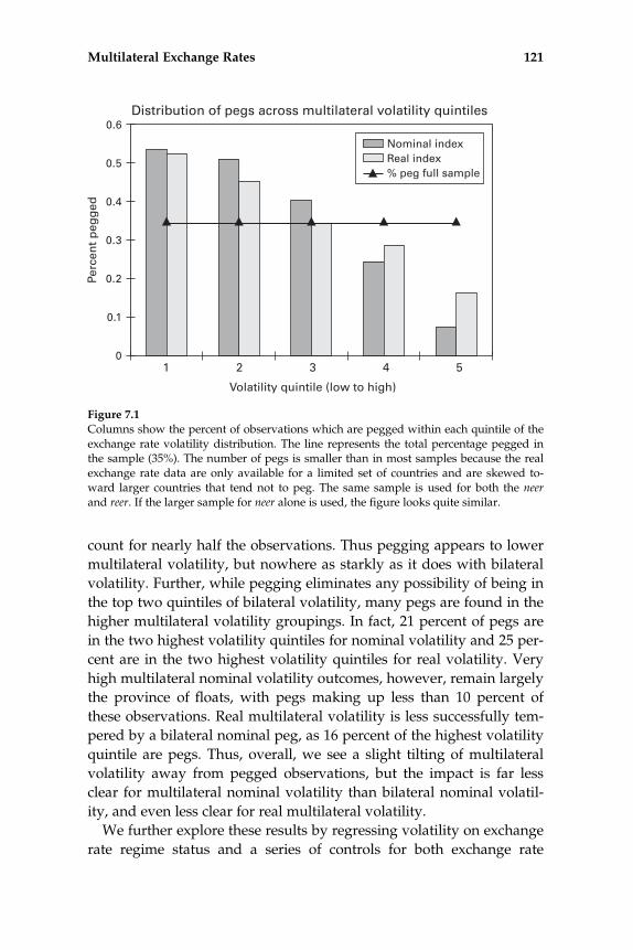
count for nearly half the observations. Thus pegging appears to lower
multilateral volatility, but nowhere as starkly as it does with bilateral
volatility. Further, while pegging eliminates any possibility of being in
the top two quintiles of bilateral volatility, many pegs are found in the
higher multilateral volatility groupings. In fact, 21 percent of pegs are
in the two highest volatility quintiles for nominal volatility and 25 per-
cent are in the two highest volatility quintiles for real volatility. Very
high multilateral nominal volatility outcomes, however, remain largely
the province of floats, with pegs making up less than 10 percent of
these observations. Real multilateral volatility is less successfully tem-
pered by a bilateral nominal peg, as 16 percent of the highest volatility
quintile are pegs. Thus, overall, we see a slight tilting of multilateral
volatility away from pegged observations, but the impact is far less
clear for multilateral nominal volatility than bilateral nominal volatil-
ity, and even less clear for real multilateral volatility.
We further explore these results by regressing volatility on exchange
rate regime status and a series of controls for both exchange rate
Figure 7.1
Columns show the percent of observations which are pegged within each quintile of theexchange rate volatility distribution. The line represents the total percentage pegged inthe sample (35%). The number of pegs is smaller than in most samples because the realexchange rate data are only available for a limited set of countries and are skewed to-ward larger countries that tend not to peg. The same sample is used for both the neerand reer. If the larger sample for neer alone is used, the figure looks quite similar.
Multilateral Exchange Rates 121
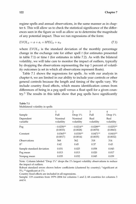
regime spells and annual observations, in the same manner as in chap-
ter 6. This will allow us to check the statistical significance of the differ-
ences seen in the figure as well as allow us to determine the magnitude
of any potential impact. Thus we run regressions of the form:
EVOLit ¼ aþ ai þ bPEGit þ uit (7.1)
where EVOLit is the standard deviation of the monthly percentage
change in the exchange rate for either spell t (for estimates presented
in table 7.1) or time t (for estimates in table 7.2). As with the bilateral
volatility, we will take care to monitor the impact of outliers, typically
by dropping the observations representing the top 1 percent of volatil-
ity outcomes (a set in which all observations represent floats).
Table 7.1 shows the regressions for spells. As with our analysis in
chapter 6, we are limited in our ability to include year controls or other
general controls because the length and timing of the spells vary. We
include country fixed effects, which means identification comes from
differences of being in a peg spell versus a float spell for a given coun-
try.5 The results in this table show that peg spells have significantly
Table 7.1
Multilateral volatility in spells
Sample1Full
2Drop 1%
3Full
4Drop 1%
Dependentvariable
Nominalvolatility
Nominalvolatility
Realvolatility
Realvolatility
Peg �0.0250** �0.0214** �0.0289** �0.0253**(0.0033) (0.0028) (0.0070) (0.0063)
Constant 0.0365** 0.0330** 0.0471** 0.0410**(0.0017) (0.0014) (0.0035) (0.0032)
Observations 568 562 318 314
R2 0.42 0.45 0.37 0.43
Sample standard deviation 0.031 0.025 0.058 0.043
Peg mean 0.013 0.013 0.020 0.017
Nonpeg mean 0.035 0.032 0.045 0.039
Note: Column labeled ‘‘Drop 1%’’ drops the 1% largest volatility observations to reducethe impact of outliers.Robust standard errors shown below coefficients (clustered by country); * significant at5%; **significant at 1%.Country fixed effects are included in all regressions.Sample: 119 countries from 1979–2004 for columns 1 and 2; 68 countries for columns 3and 4.
122 Chapter 7

lower multilateral volatility than float spells, even when we control for
all differences across countries with country fixed effects. We see that
the estimated coefficient on the peg variable is negative and highly sig-
nificantly different from zero.6 Pegs have a mean nominal volatility of
0.013 and nonpegs roughly 0.035, and hence in a simple regression,
the coefficient on peg is �0.025.7 The coefficients on peg for real and
nominal volatility are very close, but the overall volatility outcomes
have a slightly larger range for the real volatility (the standard devia-
tion of volatility in the sample is higher). Thus the impact on volatil-
ity—relative to the variance of volatility—is slightly smaller for real
multilateral volatility.
We can control for more features of the data by analyzing annual
observations rather than spells. For example, we can take into account
the possibility that many first-year floats may be crisis observations,
and hence atypical. We can also control for various annual covariates
like inflation, capital controls, and year effects. Table 7.2 shows the
results.8 With just the peg and country fixed effects included, the esti-
mated peg coefficient is 70 percent of the standard deviation of nomi-
nal volatility and 40 percent of the standard deviation of real volatility
in the respective regressions. In both cases the coefficient is highly sta-
tistically significantly different from zero.9
The coefficients on the first year of floating variable show that vola-
tility is higher immediately after a peg breaks. But, even controlling
for this high volatility first year of floating, pegs are still considerably
less volatile than floats. Thus floats are not simply more volatile be-
cause of crises observations following a peg; rather both nominal and
real multilateral exchange rate volatilities are lower for pegs (also recall
that these results do not include the very high volatility observations).
This result still holds when controlling for both inflation and capital
controls, as demonstrated in the regressions presented in columns 3
and 6. These regressions also show that high-inflation countries have
significantly more nominal and real volatility, but capital controls do
not significantly affect volatility.10
This significant effect of inflation on multilateral volatility could sug-
gest that any sensible macro policy, and not just pegging, lowers multi-
lateral volatility. Rose (2007) argues that countries that target inflation
do not face higher volatility than a control group of countries. To ex-
plore this issue, we examine the multilateral exchange rate behavior of
countries that have inflation targets, countries that peg, and countries
that float.
Multilateral Exchange Rates 123
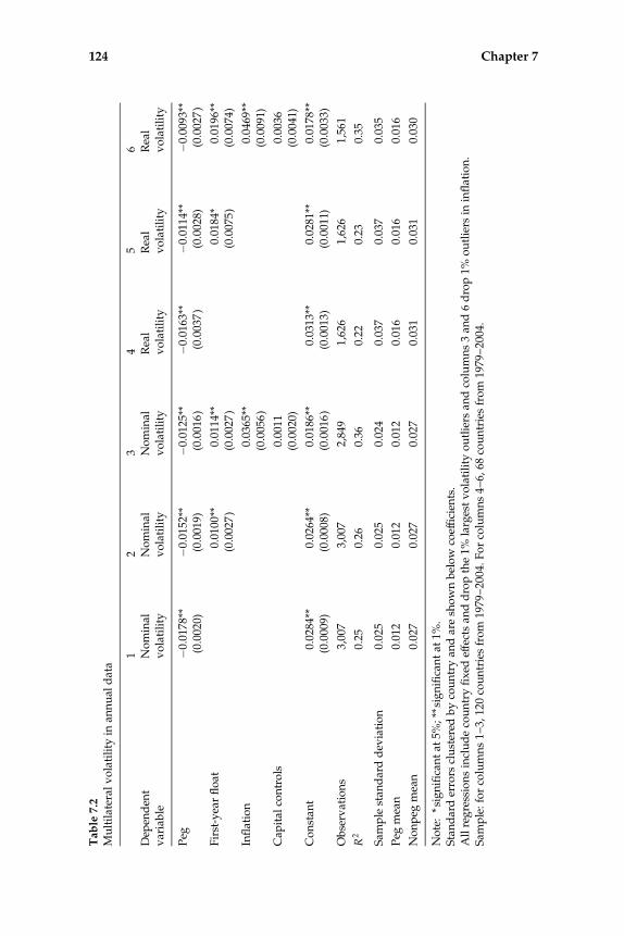
Table
7.2
Multilateral
volatility
inan
nual
data
Dep
enden
tvariable
1 Nominal
volatility
2 Nominal
volatility
3 Nominal
volatility
4 Real
volatility
5 Real
volatility
6 Real
volatility
Peg
�0.017
8**
�0.0152**
�0.012
5**
�0.0163**
�0.0114**
�0.009
3**
(0.002
0)(0.001
9)(0.001
6)
(0.003
7)
(0.002
8)(0.002
7)
First-yearfloat
0.0100
**0.01
14**
0.0184
*0.01
96**
(0.002
7)
(0.002
7)
(0.007
5)
(0.007
4)
Inflation
0.0365**
0.0469
**(0.005
6)
(0.009
1)
Cap
ital
controls
0.00
110.00
36(0.002
0)(0.004
1)
Constan
t0.02
84**
0.0264
**0.01
86**
0.0313
**0.0281
**0.01
78**
(0.000
9)(0.000
8)(0.001
6)
(0.001
3)(0.001
1)(0.003
3)
Observations
3,007
3,007
2,849
1,626
1,626
1,561
R2
0.25
0.26
0.36
0.22
0.23
0.35
Sam
ple
stan
darddev
iation
0.025
0.025
0.024
0.037
0.037
0.035
Peg
mean
0.01
20.012
0.01
20.016
0.016
0.01
6
Nonpeg
mean
0.02
70.027
0.02
70.031
0.031
0.03
0
Note:*significantat
5%;**significantat
1%.
Standarderrors
clustered
bycountryan
dareshownbelow
coefficien
ts.
Allregressionsincludecountryfixed
effectsan
ddropthe1%
largestvolatility
outliers
andcolumns3an
d6drop1%
outliers
ininflation.
Sam
ple:forcolumns1–3,
120countriesfrom
1979
–2004.Forcolumns4–6,
68countriesfrom
1979
–2004.
124 Chapter 7

Figure 7.2 shows that observations associated with a pegged ex-
change rate have lower median volatility than both observations asso-
ciated with a floating exchange rate and observations representing
years in which countries target inflation. Countries that target inflation
do not appear to have more volatility than a typical float (as Rose sug-
gests), but this method of reducing inflation and stabilizing monetary
policy does not have the same impact on multilateral volatility as peg-
ging the exchange rate.
Table 7.3 extends these results by testing inflation targeting in the
broader regressions shown in table 7.2. Controlling for inflation tar-
geting makes no difference to the results—the coefficient on peg is
unchanged from table 7.2—and the coefficient on inflation targeting is
not significantly different from zero. Rose’s results suggest that coun-
tries that target the inflation rate are not different than a typical coun-
try. Here we see, however, that volatility is higher during episodes of
inflation targeting than during years in which a country pegs its ex-
change rate, but is not significantly different from years in which a
country’s currency floats. When controlling for first-year floating, infla-
tion, and capital controls, the coefficient on the peg is also the same as
in table 7.2. When controlling for inflation, countries that target infla-
tion show slightly elevated nominal exchange rate volatility (column
2). One reason they have low volatility is that they have low inflation,
so controlling for low inflation may cloud the results.
Figure 7.2
Median volatility across policy regimes.
Multilateral Exchange Rates 125
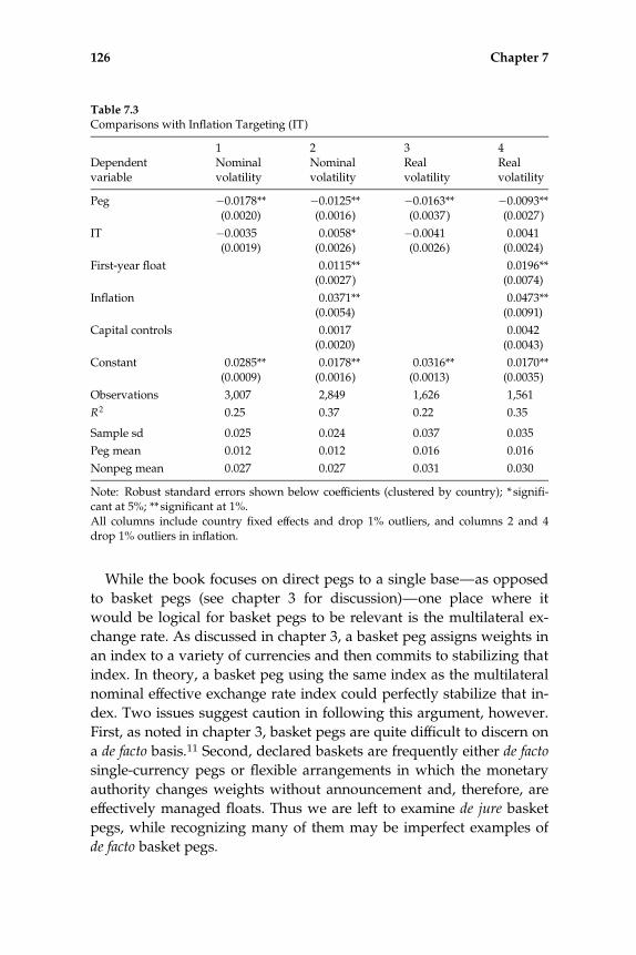
While the book focuses on direct pegs to a single base—as opposed
to basket pegs (see chapter 3 for discussion)—one place where it
would be logical for basket pegs to be relevant is the multilateral ex-
change rate. As discussed in chapter 3, a basket peg assigns weights in
an index to a variety of currencies and then commits to stabilizing that
index. In theory, a basket peg using the same index as the multilateral
nominal effective exchange rate index could perfectly stabilize that in-
dex. Two issues suggest caution in following this argument, however.
First, as noted in chapter 3, basket pegs are quite difficult to discern on
a de facto basis.11 Second, declared baskets are frequently either de facto
single-currency pegs or flexible arrangements in which the monetary
authority changes weights without announcement and, therefore, are
effectively managed floats. Thus we are left to examine de jure basket
pegs, while recognizing many of them may be imperfect examples of
de facto basket pegs.
Table 7.3
Comparisons with Inflation Targeting (IT)
Dependentvariable
1Nominalvolatility
2Nominalvolatility
3Realvolatility
4Realvolatility
Peg �0.0178** �0.0125** �0.0163** �0.0093**(0.0020) (0.0016) (0.0037) (0.0027)
IT �0.0035 0.0058* �0.0041 0.0041(0.0019) (0.0026) (0.0026) (0.0024)
First-year float 0.0115** 0.0196**(0.0027) (0.0074)
Inflation 0.0371** 0.0473**(0.0054) (0.0091)
Capital controls 0.0017 0.0042(0.0020) (0.0043)
Constant 0.0285** 0.0178** 0.0316** 0.0170**(0.0009) (0.0016) (0.0013) (0.0035)
Observations 3,007 2,849 1,626 1,561
R2 0.25 0.37 0.22 0.35
Sample sd 0.025 0.024 0.037 0.035
Peg mean 0.012 0.012 0.016 0.016
Nonpeg mean 0.027 0.027 0.031 0.030
Note: Robust standard errors shown below coefficients (clustered by country); * signifi-cant at 5%; ** significant at 1%.All columns include country fixed effects and drop 1% outliers, and columns 2 and 4drop 1% outliers in inflation.
126 Chapter 7

In table 7.4 we augment our basic regressions on annual data with
dummy variables for a declared basket peg. The results show that for
both nominal and real multilateral volatility the basket pegs have a
much smaller impact on volatility than a direct peg to a base. Thus, ei-
ther because the basket is simply declared but not actually stabilized,
or because the basket is not matched to the trade weighted index, mul-
tilateral pegs are less effective than direct pegs at stabilizing the ex-
change rate. For example, the results in column 1 include a dummy for
a de jure basket peg, and thus represent a direct parallel to the regres-
sion in column 1 in table 7.2. The coefficient on the basket peg is close
to zero and statistically insignificant. This specification, however, is
asking whether basket pegs have lower volatility than all other ex-
change rate arrangements.
A distinct question is whether basket pegs have lower volatility than
floats. This requires controlling for direct pegs. But we need to account
for the fact that 134 out of the 512 declared basket pegs are also de facto
direct pegs. For example, Jordan declared a basket peg from 1989 to
1997 but also had a de facto peg to the US dollar from 1990 to 1997
(including two years with precisely zero change against the dollar).
We thus include three separate dummies: direct pegs that are not
declared baskets; declared baskets that are not direct pegs; and direct
pegs that are declared baskets. In this specification we see that
declared baskets that are not actually direct pegs do show less volatil-
ity than floats (the coefficient is significant and negative), but the im-
pact is less than half of a direct peg. Direct pegs—whether or not
declared as baskets—both show significantly less volatility than either
floats or declared baskets. When controlling for other factors, such as
capital controls, inflation, and first year of floating, the pattern is the
same.
When we consider real effective exchange rate volatility, the basket
pegs have no statistically significant impact regardless of controls, or
whether we compare them to all other exchange rate arrangements, or
only compare them to floats. The coefficient on the declared basket
pegs and on the declared basket pegs that do not qualify as direct pegs
are never statistically significantly different from zero, and the point
estimates are always close to zero. These results, in part, justify the
book’s emphasis on the direct pegs to single currencies (or systems of
fixed exchange rates). Basket pegs are difficult to verify and in many
cases seem to differ little from either a direct peg (if the basket is
weighted heavily to one country) or managed floating (if it is changed
Multilateral Exchange Rates 127
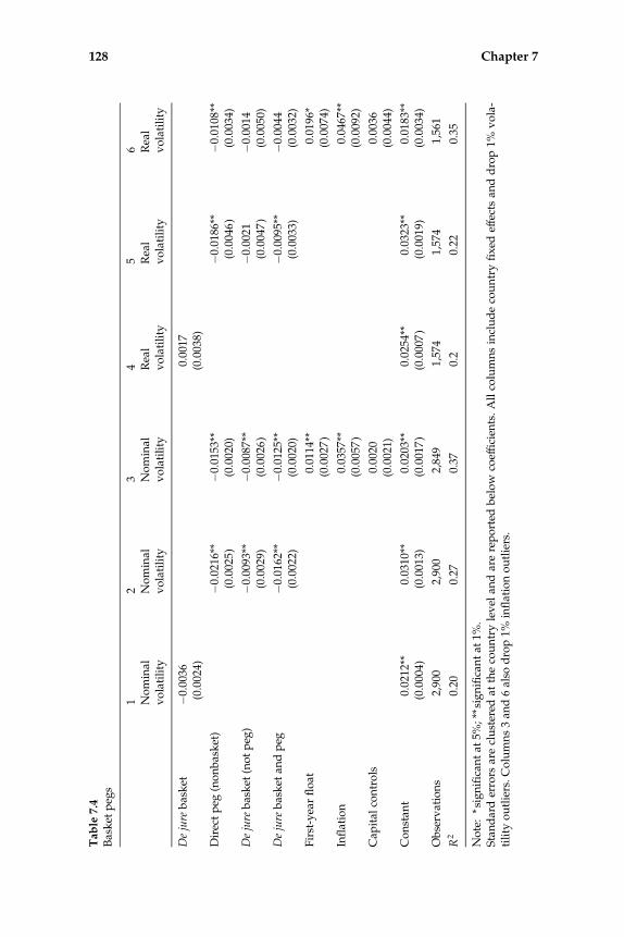
Table
7.4
Basket
peg
s
1 Nominal
volatility
2 Nominal
volatility
3 Nominal
volatility
4 Real
volatility
5 Real
volatility
6 Real
volatility
Dejure
basket
�0.0036
0.0017
(0.002
4)(0.003
8)
Directpeg
(nonbasket)
�0.021
6**
�0.0153**
�0.0186**
�0.010
8**
(0.002
5)
(0.002
0)(0.004
6)
(0.003
4)
Dejure
basket
(notpeg
)�0
.009
3**
�0.0087**
�0.0021
�0.001
4(0.002
9)(0.002
6)
(0.004
7)
(0.005
0)
Dejure
basket
andpeg
�0.016
2**
�0.0125**
�0.0095**
�0.004
4(0.002
2)(0.002
0)(0.003
3)(0.003
2)
First-yearfloat
0.0114
**0.01
96*
(0.002
7)
(0.007
4)
Inflation
0.0357
**0.0467
**(0.005
7)
(0.009
2)
Cap
ital
controls
0.0020
0.00
36(0.002
1)(0.004
4)
Constan
t0.0212
**0.03
10**
0.0203
**0.0254
**0.0323
**0.01
83**
(0.000
4)(0.001
3)(0.001
7)
(0.000
7)
(0.001
9)(0.003
4)
Observations
2,900
2,900
2,849
1,574
1,574
1,561
R2
0.20
0.27
0.37
0.2
0.22
0.35
Note:*significantat
5%;**significantat
1%.
Standarderrors
areclustered
atthecountrylevel
andarereported
below
coefficien
ts.Allcolumnsincludecountryfixed
effectsan
ddrop1%
vola-
tility
outliers.Columns3an
d6also
drop1%
inflationoutliers.
128 Chapter 7

often). Thus, strikingly, simply pegging to one currency has a bigger
and more significant impact on multilateral exchange rate volatility
than a basket peg.
Overall, these results show that the multilateral volatility of both real
and nominal exchange rates is lower when a country pegs than when it
floats. This is true even when controlling for country effects, outliers, or
many other features and policies.12
We close this chapter by briefly considering whether these results for
the contemporaneous effect of pegs on multilateral volatility extend
over time, along the lines of our inquiry in the previous chapter. Figure
7.3 repeats the exercise of figure 6.2 and examines volatility outcomes
in years after a pegged observation, regardless of whether a country
stays pegged. This represents the best guess of future volatility for an
observer knowing nothing more than the fact that the country is
Figure 7.3
Time 0 represents the contemporaneous coefficient of exchange rate volatility on pegging,time 1 represents the coefficient on a lagged peg, and so on. Thus the point at time 2 rep-resents the difference in volatility for a country that was pegged two years ago (whetheror not it has remained pegged). Country- and year-fixed effects are included. The darklines represent 2 times standard error bands around the main point estimates where stan-dard errors are clustered on country. To ensure that the comparison is with nonpeggedobservations, new pegs that are not re-pegs are excluded. The squares represent pointestimates if the first year of pegging is excluded.
Multilateral Exchange Rates 129

pegged today. We see in figure 7.3 that, while a pegged observation
has lower nominal multilateral volatility in the year it is pegged, the
likelihood of a break in the peg—combined with the relatively weak
impact of pegging—means that just one year out, multilateral volatility
is not necessarily lower, and two years out there is no distinguishable
impact—on average—for pegs versus floats. Even dropping the first
year of pegging (and hence dropping the unstable single-year pegs)
has little impact.
7.3 Conclusion
By definition, an exchange rate can only be fixed against one currency.
The results in chapter 6 show that fixed exchange rates lower bilateral
volatility. But this result has limited implications for the economic
effects of pegging. Many economic outcomes depend more on the mul-
tilateral exchange rate than the bilateral exchange rate. This chapter
shows that a peg does stabilize the multilateral exchange rate relative
to a nonpeg. Unlike bilateral volatility, pegs are not the only observa-
tions with low volatility. Many nonpegged observations have very
low multilateral volatility. Also many pegged observations have high
volatility. Thus pegging is neither necessary for low multilateral vola-
tility nor is it a guarantee for low volatility. But the typical peg has
lower volatility than the typical float even when we control for country
effects and other behavior, meaning that a given country has lower
multilateral volatility when it is pegging. The effect of the peg on vola-
tility is stronger than that of other policies that might generate broad
macro stability, such as inflation targeting or pegging to a basket of
currencies. The latter result is particularly surprising since one might
expect that a basket peg stabilizes the multilateral rate completely. It
suggests that de jure baskets either do not truly follow the basket or
the basket weights do not match the trade weights.
Overall, the results in chapters 6 and 7 show that exchange rate
regimes do have a material impact on the exchange rate. Pegging sta-
bilizes the bilateral rate in a substantial way relative to floats. This dif-
ference in volatility spills over into multilateral volatility as well. Thus
it seems reasonable that exchange rate regimes may have impacts on
other macroeconomic outcomes. We turn to these topics in chapters 8
through 11.
130 Chapter 7
IV Economic Consequences of Exchange RateRegimes


8 Exchange Rate Regimes and Monetary Autonomy
The greater the attention given to the exchange rate, the more constrainedmonetary policy is in pursuing other goals.
—Maurice Obstfeld, ‘‘The global capital market, benefactor or menace,’’ 1998
Chapter 2 introduced the concept of the trilemma. A country cannot
pursue more than two of the three options of a fixed exchange rate,
open financial markets, and domestic monetary autonomy. This core
concept of international macroeconomics is very general, and it is
an implication of a wide range of macroeconomic models that allow
for international trade in assets, but it also follows from fairly basic
intuition.
The trilemma is sometimes summarized to mean that countries can
operate with an open capital market, a peg and zero autonomy; a
closed capital market, a peg with autonomy; or an open capital market,
a float with autonomy. More accurately, however, the concept is about
trade-offs. A country does not have to operate purely at any of these
corner solutions, but if it wants to stabilize the exchange rate and allow
some capital mobility, some compromise in domestic monetary auton-
omy will be necessary. Countries can give up varying amounts of all
three options, the only stricture being they cannot pursue all three at
the same time.
The focus of this chapter is the important question of whether the
predictions of the theory of the policy trilemma tend to be borne out in
practice. We will present tests that focus on the extent to which there is
a systematic difference in monetary policy independence across sets of
countries according to their exchange rate and capital mobility policies.
In particular, we focus on whether exchange rate pegs limit monetary
autonomy. As is the case with other exchange rate issues, countries’
experiences during the modern era offer an interesting and useful sam-
ple for these tests due to the heterogeneity of policies during this pe-
riod. We can also use tests based on the gold standard era and Bretton
Woods era to provide context for the results of the modern era.
8.1 Exchange Rates, Interest Rates, and the Policy Trilemma1
Before presenting empirical tests, we discuss the general principle of
the trilemma, the link between exchange rates and interest rates under
a peg with capital mobility. If investors can move money to either of
two countries (open financial markets), and they believe that the price
of one currency for the other will stay constant over time (fixed ex-
change rates), then the only way for there to be equilibrium in the ex-
change rate market is if the interest rate is the same in both countries.
If a riskless asset paid more in country A than in country B, and the ex-
change rate at the end of the period will be the same as the one at the
start, there would be no reason to ever hold the lower return country
B asset. Everyone would try to sell the asset in country B and change
their money to country A’s currency—causing an increase in the price
of country A’s currency and hence the exchange rate peg to break.2
Thus we expect the interest rate in one country to equal the interest
rate in the other when there is a peg.
Alternatively, if the exchange rate is not fixed, interest rates do not
have to be equivalent across countries. If an investor expects country
B’s currency to be worth less at the end of the year by 5 percent, she
would no longer want to hold country B’s asset in her portfolio unless
she received an extra 5 percent in interest over the year to compensate
her for the loss in value due to the depreciation of the foreign currency,
which causes the domestic-currency price of the foreign asset to de-
crease by 5 percent. Thus, if a country has a fixed exchange rate, but
people worry it may not last, there may be higher rates in the pegged
country than in the base.
An equation that captures these ideas is the familiar uncovered inter-
est parity relationship,
R ¼ R*þ%DEe, (8.1)
where %DEe represents the expected change in the exchange rate over
the maturity of the bonds. The equation implies that the home interest
rate R must equal the foreign interest rate R* plus any expected depre-
ciation in the home currency. If this condition is satisfied, investors
134 Chapter 8

expect to earn the same amount of money in either country, and thus
there is no excess demand in one direction or the other. Capital mobil-
ity is a precondition for the equation to hold; that is, the ability to pur-
chase foreign bonds is a relevant consideration for the domestic
investor. It is, of course, possible that new information will appear and
expectations will have been wrong, but we expect this equation to hold
on average. If currencies are floating, then %DEe represents the
expected depreciation; if they are pegged, then we can think of it as
encompassing some probability of breaking the peg combined with
the expected extent of a depreciation if the peg breaks. Thus, if there is
some chance of the peg breaking, we will not expect R ¼ R* to hold
perfectly.
In addition, if the assets are not identical, we do not expect R and R*
to be the same even if there is no chance of a depreciation or a devalu-
ation. Consider a comparison of US Treasury bills (highly unlikely to
default) and Argentinean Treasury bills (likely to default) in late 2001.
The Argentine bonds are more risky and would have to pay a higher
interest rate due to a higher ‘‘risk premium’’ on the Argentine bonds.
Thus we expect R to equal R* plus any expected depreciation and
any risk premium. Therefore we would not conduct an empirical test
of the trilemma that requires interest rates to be identical. Rather, an
appropriate test would examine whether the interest rate of countries
that peg move one-for-one with the foreign or base interest rate. This
test allows for a gap in the levels on interest rates across countries, and
assumes that the risk premium and the odds of a peg breaking are rel-
atively static, or at least do not change systematically with changes in
the base interest rate. The regression specification for such a test is
DR ¼ aþ bDR*. (8.2)
We expect b to equal 1 for a sample of pegged countries with open
financial markets. If an increase in the base interest rate makes it more
likely that the home country will break its peg (because the home
country may not want to raise its interest rate), depreciation expecta-
tions rise when R* rises. In this case, R would have to increase by
more than R* to preserve the peg, and b would be greater than one.
On the other hand, as we have noted before, pegs are rarely perfectly
fixed, but tend to have some small room for discretion. Thus countries
may be able to allow a small depreciation if R* goes up, rather than re-
spond entirely with interest rate changes. If this is the case, b may be
less than one.
Monetary Autonomy 135
For a sample of floating countries, we may expect a b of zero. This
would be the case if floating countries ignored the base interest rate
when setting monetary policy and their economies were independent.
On the other hand, countries may experience common shocks. In this
case they may coincidentally increase or decrease interest rates to-
gether such that b is greater than zero. In addition floats may try to
temper exchange rate changes and hence respond to changes in the
base interest rate to try to partially stabilize the exchange rate. This
‘‘fear of floating’’ behavior will also generate a b greater than zero.
Capital controls are crucial to this discussion. A country that limits
capital flows and administratively sets the price of the exchange rate
has a wide latitude in setting its interest rate since capital controls pre-
vent international capital flows from forcing a break in the exchange
rate peg. Thus the expected response of home interest rates to the base
interest rate outlined in this section would hold—or at least would
hold most strongly—for countries with open capital markets.
8.2 Literature on the Trilemma
While the general prescriptions of the trilemma fall straight from basic
theory, room for discretion provided by target zones or transaction
costs could limit the loss of autonomy from pegging. On the other
hand, even floating countries may have a limited amount of autonomy
if there is a correlation of depreciation expectations or risk premia with
the base interest rate in which case countries may follow the base to
some extent to avoid large movements in the exchange rate even if
they are floating. Thus the extent that a fixed exchange rate truly limits
monetary autonomy becomes an empirical question.
Both possible caveats to the trilemma have been explored empiri-
cally. The first question—is there really enough room for discretion to
make the constraint irrelevant?—has been explored chiefly in the gold
standard era. Work by Bordo and MacDonald (1997) suggested that
countries on the gold standard had some flexibility in their monetary
policy. These results are considered by Obstfeld, Shambaugh, and Tay-
lor (2005), who show that, while the trilemma does not bind entirely,
there is still a significant difference between the loss of monetary policy
autonomy under pegs as compared to under floats. More recently Jan-
sen (2008) argues that the Dutch still had some limited autonomy de-
spite pegging to Germany due to its tight target zone against the
deutsche mark and argues a target zone can provide some autonomy.
136 Chapter 8
Alternatively, the fear of floating school of thought suggests that
even countries that do not truly peg have limited monetary policy au-
tonomy (see chapters 4 and 6). It is important to make a distinction in
this argument. If one simply claims that some countries declare a float
but actually peg, and those countries lose autonomy, this is not evi-
dence against the trilemma but just reflects mis-declaration of the true
exchange rate regime, as noted in chapter 3. The real question of the
trilemma is to what extent actually following a peg limits monetary au-
tonomy. Fear of floating is relevant to the trilemma if countries that
actually do float still manage their exchange rates and give up auton-
omy as a result.
Some research points to a failure of empirical support for the policy
trilemma. Frankel (1999) suggests that, in some cases, floats may fol-
low the base rate even more than pegs. Frankel, Schmukler, and Serven
(2004) suggest that their results show limited autonomy for all but the
largest floating countries. Forssbæck and Oxelheim (2006) examine EU
nations in the 1979 to 2000 period and argue there is not clear evidence
of monetary policy constraints differing across exchange rate regimes.
But they focus on testing elasticities rather than more straightfor-
wardly testing differences in interest rates. This leads to very large
error bands around the results, and thus they cannot reject any reason-
able null hypothesis about the data.
Other research supports the empirical relevance of the policy tri-
lemma. Shambaugh (2004) and Obstfeld, Shambaugh, and Taylor
(2005) suggest that the gap between pegs and floats becomes clear
when actual pegs and floats are carefully distinguished and when us-
ing an empirical specification appropriate for the time-series properties
of the data and eliminating hyperinflation countries. Floating countries
appear to respond less, and with more delay, to movements in the base
rate. Clarida, Gali, and Gertler (1999) analyze whether the policy inter-
est rate of different major countries is driven by local conditions or in-
ternational interest rates. They find that while the United States,
Germany, and Japan (all floaters) follow their own shocks, even large
countries participating in the EMS significantly curtail the extent that
they follow their own shocks and instead follow the German interest
rate.3
Other recent research has tried to consider the type of interest rate
shock coming from the base country. Basic theory suggests that any in-
terest rate movement by the base country should be followed by a
pegged country. Much research on monetary policy, though, prefers to
Monetary Autonomy 137

eliminate any ‘‘endogenous’’ monetary policy changes—where the cen-
tral bank is responding to local conditions. If one worried that some
countries more naturally followed the base country interest rate due
to similar economic circumstances (more common shocks), one might
prefer to see responses to exclusively exogenous monetary policy
shocks. Borenzstein, Zettelmeyer, and Philippon (2001) examine the
responsiveness of a variety of countries to identified US monetary
policy shocks. They find that Hong Kong reacts more than Singapore
though Mexico and Argentina are somewhat similar. In addition they
find that Hong Kong responds significantly more to exogenous US in-
terest rate movements than a variety of industrial countries, which is
consistent with pegging generating a loss of monetary autonomy. Min-
iane and Rogers (2007) derive monetary policy shocks based on a vec-
tor autoregression, and while their results are focused on the capital
control side of the trilemma, their results regarding exchange rate
regimes are also supportive of the idea that pegged open financial mar-
ket countries follow base shocks more closely. Bluedorn and Bowler
(2008) describe in detail how correlations between the base interest
rate and exchange rate expectations may vary depending on the char-
acter of the interest rate change (whether or not it was expected and
whether it responded to economic conditions or was exogenous). Their
results suggest that open capital market pegs may respond even more
strongly to exogenous shocks to the base interest rate.
We next consider results that test the basic premises of the trilemma
described in section 8.1. These results are based on results in Sham-
baugh (2004) and Obstfeld, Shambaugh, and Taylor (2005).
8.3 Empirical Evidence on the Trilemma
In this section we present tests of monetary autonomy across different
exchange rate policy regimes. We use the co-movement of home and
base-country interest rates as an indicator of monetary autonomy. The
exchange rate regime status is based on the de facto Shambaugh (2004)
classification.4 We also employ a measure of capital controls from the
IMF annual yearbooks since, as discussed above, the exchange rate—
interest rate trade-off is most relevant for countries with open capital
markets.5
We test the basic equation outlined in section 8.1 across different
types of exchange rate regimes. Our focus is on the modern era (as in
Shambaugh 2004), a time period where there is adequate variability in
138 Chapter 8

regimes to test different arrangements. We also present results from the
Bretton Woods and gold standard periods (as in Obstfeld, Shambaugh,
and Taylor 2005). These earlier eras provide helpful benchmarks and a
useful context because many countries took similar positions within
the trilemma framework during these periods.6 In the gold standard
era most countries were pegged and there were no capital controls,
while during the Bretton Woods period most countries pegged but
capital controls were pervasive. In contrast, the modern era is marked
by a mixture of policy regimes.
Each of these three eras demands its own method for classifying
observations as either pegs or floats. For the gold standard era, coun-
tries are considered pegged if they have a stable exchange rate against
gold. Thus, for the gold standard era, we use a de facto gold peg classi-
fication that parallels those used in the Bretton Woods era and the
modern era. The base interest rate for the gold standard era is the UK
interest rate (the London call money rate) because sterling was consid-
ered the base currency at that time. Home interest rates are call money
rates for a variety of countries from 1878 to 1914. For the Bretton
Woods era, the base interest rate is the US dollar interest rate since the
United States was the center country in the Bretton Woods system (the
sample that we use for this period is from 1959 to 1970). Obstfeld,
Shambaugh, and Taylor (2005) provide details of the data for these
eras. The modern era involves a variety of base interest rates as differ-
ent countries peg to different bases in this era (the sample for this
period is 1973 to 2000, as in Shambaugh 2004).7
The basic analysis examines the changes in annual interest rates
across a panel of countries using OLS regressions. Results in figure 8.1
present the b coefficients (and the associated 95 percent confidence
intervals) from the regressions based on equation 8.2 for a panel of
countries across each of the three eras.8 We expect the b coefficient to
be larger (and near 1) for the estimates using the gold standard era
sample, when countries pegged to gold and there were few constraints
on international capital flows, and, to be close to zero for estimates
using the Bretton Woods era sample, when there were significant capi-
tal controls. The legend to this figure reports the R2 statistics for these
regressions; we expect these to be higher for periods when the domi-
nant determinant of the home interest rate is the base interest rate. The
results in this figure match these expectations. For the gold standard
countries, countries follow the base to a large degree and a reasonable
portion of interest rate changes can be explained by changes in the
Monetary Autonomy 139

base. In the Bretton Woods period, capital controls shut down any in-
terest rate pass-through. There is a tendency for home interest rates to
follow the base interest rate in the modern era, but less of the home in-
terest rate behavior is explained by the base interest rate during this
period than in the gold standard era.
Another way to analyze the impact of the exchange rate regime on
monetary autonomy is by estimating equation (8.1) separately for pegs
and nonpegs in the gold standard and modern eras (we cannot under-
take a similar exercise for the Bretton Woods era since all countries in
our sample pegged during that time). The results of this exercise,
reported in table 8.1, again support the core idea that pegging the ex-
change rate leads to a loss of monetary autonomy. The results here are
even stronger than those represented in figure 8.1. Gold standard pegs
move with the base considerably and the R2 is quite high. On the other
hand, nonpegged countries during that era show no propensity to fol-
low the base, and the R2 is zero. The gold standard results provide an
important context for the results from the modern era. In the earlier pe-
riod, when there were no capital controls and there was strict adher-
ence to the peg, the b coefficient is only 0.5. The results in the modern
era are similar. As in the gold standard, pegged countries moved their
interest rates roughly half a point for every point move by the base.
Nonpegged countries move considerably less, although nonpegs fol-
low the base more in the modern era than in the gold standard. In ad-
Figure 8.1
Response of local interest rate to base interest rate in different eras. Figure shows the re-sponse of local rates to base rates as well as two standard error bars. The R2 for the goldstandard is 0.26, for Bretton Woods 0.02, and for the modern era 0.03.
140 Chapter 8

dition the R2 for pegged countries is substantial, but essentially zero
for nonpegs. Effectively, a change in the base interest rate has no infor-
mation about what will happen to the local interest rate for nonpegs.
Is a value of b of 0.5 too low to imply that pegs impose a meaningful
constraint on monetary autonomy? Is a statistically significant value of
b equal to 0.27 too high to imply monetary autonomy for nonpegs?
These questions are addressed by Obstfeld, Shambaugh, and Taylor
(2005). In one exercise, they generate data from a simulated target
zone model with a 2 percent band. They find that a coefficient of 0.5
and an R2 statistic below 0.2 are consistent with this tight exchange
rate band. They also find that a correlation of shocks between the
home and foreign countries can result in coefficients on the order of
0.3 even when there is a floating exchange rate and monetary auton-
omy (although the R2 statistic remains near zero in this case).
An alternative approach to this data involves pooling the sample
across pegs and nonpegs in order to check the statistical significance of
the difference in the response of R to R* across exchange rate regimes.
This involves estimating the equation:
DRit ¼ aþ b1DR*it þ b2(Pegit � DR*
it)þ e it. (8.3)
The b1 coefficient represents the extent of common shocks and fear of
floating in home interest rate movements, and the b2 coefficient reflects
monetary constraints due to pegging. This specification allows us to
test whether the response of home interest rates to base rates is signifi-
cantly different between countries that peg and countries that do not
Table 8.1
Results across exchange rate regime status
Goldstandardpeg
Goldstandardnonpeg
Modernera peg
Moderneranonpeg
DR� 0.52** 0.05 0.46** 0.27**(0.04) (0.09) (0.04) (0.08)
R2 0.41 0.00 0.19 0.01
Observations 350 140 748 1,103
Note: dependent variable: DR. Gold standard results for 1880–1914, Modern era resultsfrom Shambaugh (2004) using 150 countries from 1973–2000.Standard errors underneath coefficients. *denotes statistically significantly different fromzero at the 95% confidence level, and **denotes 99% level.See Obstfeld, Shambaugh, and Taylor (2005) for details on sample.
Monetary Autonomy 141
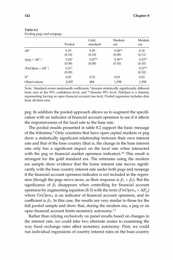
peg. In addition the pooled approach allows us to augment the specifi-
cation with an indicator of financial account openness to see if it affects
the responsiveness of the local rate to the base rate.
The pooled results presented in table 8.2 support the basic message
of the trilemma.9 Only countries that have open capital markets or peg
show a statistically significant relationship between their own interest
rate and that of the base country (that is, the change in the base interest
rate only has a significant impact on the local rate when interacted
with the peg or financial market openness indicator).10 This result is
strongest for the gold standard era. The estimates using the modern
era sample show evidence that the home interest rate moves signifi-
cantly with the base country interest rate under both pegs and nonpegs
if the financial account openness indicator is not included in the regres-
sion (though the pegs move more, as their response is b1 þ b2). But the
significance of b1 disappears when controlling for financial account
openness by augmenting equation (8.3) with the term (FinOpenit �DR*it)
where FinOpenit is an indicator of financial account openness, and its
coefficient is b3. In this case, the results are very similar to those for the
full pooled sample and show that, during the modern era, a peg or an
open financial account limits monetary autonomy.11
Rather than relying exclusively on panel results based on changes in
the interest rate, we could take two alternate routes to examining the
way fixed exchange rates affect monetary autonomy. First, we could
run individual regressions of country interest rates on the base country
Table 8.2
Pooling pegs and nonpegs
PooledGoldstandard
Modernera
Modernera
DR� 0.19 0.05 0.28** 0.18(0.10) (0.10) (0.08) (0.11)
ðpeg� DR�Þ 0.24* 0.47** 0.30** 0.33**(0.09) (0.09) (0.10) (0.10)
ðFinOpen� DR�Þ 0.31* 0.37**(0.09) (0.10)
R2 0.03 0.33 0.03 0.03
Observations 2,305 484 1,598 1,598
Note: Standard errors underneath coefficients *denotes statistically significantly differentfrom zero at the 95% confidence level, and **denotes 99% level. FinOpen is a dummyrepresenting having an open financial account (see text). Pooled regression includes datafrom all three eras.
142 Chapter 8

for different country/regime episodes and then test whether the
responsiveness to the base interest rate is altered by the exchange rate
regime. That is, for any set of years where a particular country is either
pegged or nonpegged, we label that an episode and then look at the
responsiveness of monthly interest rates to the base interest rate over
that episode. Then we can take these coefficients and see what country
characteristics drive the relationship. Shambaugh (2004) pursues this
strategy and finds that the peg variable is always a significant determi-
nant of the coefficient on the base interest rate.12
In addition we could examine the dynamics of the way local interest
rates move when the base interest rate does. To do this, we can use a
technique used first in this literature by Frankel, Schmukler, and
Serven (2004) and also by Shambaugh (2004) and Obstfeld et al. (2004,
2005). In this technique we can examine if the interest rates really move
together and also how fast the local country responds to the base coun-
try interest rates.13 Because the dynamics are almost certainly different
across individual countries, we must run these procedures on individ-
ual country episodes. We focus on a few key statistics from the results:
what is the average long run responsiveness of the local rate to the
base rate (how much of a change in the base rate is eventually passed
through to the local rate), how fast does the local rate adjust to the
base rate (specifically what is the half-life of adjustment), and what
percent of the episodes show a statistically significant relationship.
Table 8.3 presents results using this second alternative strategy. The
results show that there are no significant links between home and UK
interest rates for the few nonpegged episodes in the gold standard era.
In fact, the negative average level relationship implies that home inter-
est rates diverge from the UK rate rather than move toward it. Gold
standard pegs, on the other hand, typically have a statistically signifi-
cant relationship, and the home rate adjusts to 0.43 of any base rate
shock (consistent with the panel analysis) and the adjustment is rela-
tively quick (4–5 months). In the Bretton Woods era, far fewer pegs
are significantly linked to the base, and while the coefficient is similar,
the adjustment speed is roughly twice as high.
The analysis of the modern era divides the sample into countries that
peg, countries that do not peg, and countries that flip between these
two categories. The time samples are generally shorter (especially for
the pegs), and hence the frequency of statistical significance is lower
than in other eras. Nevertheless, we do see a levels relationship of al-
most 1 for the pegs as opposed to less than 0.7 for the flippers and a
Monetary Autonomy 143

negative relationship for the nonpegs. Similarly more pegs are statisti-
cally significant and the adjustment is faster for pegs. In general, the in-
dividual country level analysis is consistent with the panel analysis;
pegs respond more to the base than nonpegs, and tend to do so more
quickly. In short, pegs demonstrate less monetary autonomy.
The presence of the policy trilemma does not only affect monetary
policy, but economic outcomes as well. This is, in fact, closer to our ul-
timate concern. It is a topic explored by di Giovanni and Shambaugh
(2008), who base their analysis on the fact that an increase in a base
country interest rate raises the local interest rate of a pegging country.
This represents an adverse exogenous shock to the monetary policy of
that country, which leads to a reduction in growth. A similar effect
would not be expected in countries that do not peg, since interest rates
in these countries do not follow those of the base country. It is possible
for countries that do not peg to be affected by the base country rates in
other ways, but not directly through monetary policy. These results by
di Giovanni and Shambaugh show that the growth rates of pegged
countries are reduced when the base country raises rates, but that effect
is not present in countries that do not peg.
8.4 Conclusion
The policy trilemma offers an appealingly straightforward theoretical
framework. If money flows across borders and the exchange rate is
Table 8.3
Levels analysis of individual country episodes
Levelrelationship
Convergencespeed
Positive andsignificantlevels rela-tionship
Numberofepisodes
Gold standard nonpegs �0.18 4.4 months 0 5
Gold standard pegs 0.43 4.8 months 70% 20
Bretton Woods pegs 0.51 9.3 months 20% 20
Modern era pegs 0.93 7.8 months 25% 70
Modern era flips 0.68 10.6 months 16% 25
Modern era nonpegs �0.43 35.2 months 16% 32
Note: The results are from a Pesaran, Shin, and Smith test on individual country epi-sodes. The level relationship reports the average levels relationship found across theepisodes; convergence speed reports the half-life of convergence speed toward the levelsrelationship after a shock. See Obstfeld, Shambaugh, and Taylor (2005) for details onspecific episodes used.
144 Chapter 8

pegged, the return on simple bonds should be equal in the base and
pegging countries. This would limit the monetary autonomy of the
pegged country. There obviously may be benefits to pegging, but they
will come at a cost—the loss of monetary independence.
There are very important implications of this theory if it, indeed,
holds. While there has been some controversy over the empirical rele-
vance of the policy trilemma, the results presented and surveyed in
this chapter show that countries actually do face the tradeoffs associ-
ated with the trilemma. This is true both across eras and in the modern
era itself. Countries that peg, especially those with open financial mar-
kets, lose some of their monetary autonomy as compared to countries
that do not peg.
The loss of monetary autonomy is not necessarily a bad thing. A
country that has not conducted monetary policy in a responsible and
reasonable manner, and therefore would have little prospect of mone-
tary policy credibility if the central bank were left to its own discretion,
can peg in order to ‘‘import’’ the monetary policy (and credibility) of a
base country central bank. In this case, the strictures of the policy tri-
lemma may even be a blessing since forgoing monetary independence
may be welfare enhancing.14 But many countries can, and do, run sen-
sible monetary policy that responds to domestic economic conditions
and stabilizes the economy. The results in this chapter show that this
option is not open to countries with fixed currencies that allow for in-
ternational financial flows.
Monetary Autonomy 145


9 Exchange Rate Regimes and International Trade
Freely fluctuating exchanges . . . create an element of risk which tends to dis-courage international trade. The risk may be covered by ‘‘hedging’’ operationswhere a forward market exists; but such insurance, if obtainable at all, is ob-tainable only at a price and therefore generally adds to the cost of trading.1
—Ragnar Nurkse, 1944
The creation of a single currency area would add to the potential benefits of anenlarged economic area because it would remove intra-Community exchangerate uncertainties and reduce transactions costs, eliminate exchange rate vari-ability and reduce the susceptibility of the Community to external shocks.2
—Committee for the Study of Economic and Monetary Union (Delors Commit-tee), 1989
Slogans are meant to rally opinion, not to reflect subtleties. Thus the
slogan ‘‘One market, one money’’ was an effective, if not totally con-
vincing, call by the European Commission for a single currency in Eu-
rope in order to solidify the continent’s trade integration.3 At the time
the 1989 Delors Report was prepared by the European Commission
(headed by its president, Jacques Delors), there was actually little sys-
tematic empirical evidence that a single currency would promote inter-
national trade.
The empirical regularity that the slogan did reflect was the long-
standing view of the importance of exchange rate stability in Europe.
The memory of the competitive devaluations of the interwar period,
and the collapse of trade at that time, cast a long shadow over thinking
about European economic issues. The 1944 quote from Ragnar Nurkse
above demonstrates the concern that exchange rate fluctuations would
adversely affect trade. As noted in chapter 2, this concern contributed
to the establishment of the Bretton Woods bilateral dollar pegs. From a
European perspective, these bilateral dollar pegs had the detrimental

effect of limiting monetary policy autonomy in Europe (as discussed in
the previous chapter), but they also had the salutary effect of fixing Eu-
ropean cross-exchange rates. This was seen as contributing to the ex-
pansion of European trade during the postwar period, which in turn
was viewed as contributing to both prosperity and peace.
For these reasons there was a quick response in Europe to the col-
lapse of the Bretton Woods system in an effort to stave off exchange
rate instability among the continent’s countries. Initial efforts, however,
were either short-lived or limited in their membership. But with the es-
tablishment of the European Monetary System in March 1979, coun-
tries began their long, fitful march toward a single currency. The 1989
Delors Report proposed a way toward this goal, and, as shown in the
quote above, reasons to rally around its achievement. Despite many
skeptics the euro did replace national currencies, beginning with the
establishment of the European Central Bank in January 1999. At the
time of this writing the euro serves as the common currency for 16
countries.4
Is trade among these sixteen European countries larger than would
otherwise be the case just because each uses the same currency? More
broadly, do fixed exchange rates promote trade? Nurkse offers reasons
why this might be the case, and almost five decades later, the Delors
Report echoed these ideas. Contracts specifying quantities and prices
of international transactions are written up to a year before delivery
and payment takes place. This lead time is not necessarily different
from transactions that take place between a buyer and seller within a
country, but exchange rate fluctuations introduce an element of uncer-
tainty into international transactions absent from those that take place
within the borders of a single country. For example, a contract specify-
ing the dollar price of future US exports to the United Kingdom leaves
the price in terms of pounds open to the vagaries of the foreign ex-
change market. Hedging against this risk through the use of forward
markets is a possibility, but as noted by Nurkse, this hedging comes at
a price, and besides, these forward contracts are not available for many
currencies and for time horizons of more than one year. A central con-
cern is that due to this uncertainty and the associated riskiness, ex-
change rate volatility diminishes trade. As with any other feature of
an economy that adversely affects transactions, market volatility can
lower welfare.
This is a reasonable view of the effects of exchange rate volatility on
trade. But it was not one that was supported by empirical analysis dur-
148 Chapter 9

ing the first quarter century of the modern era. During all this time,
analysis of this topic proceeded by estimating trade equations that
were augmented with a term representing exchange rate volatility.
This research consistently failed to find a compelling adverse effect of
exchange rate volatility on imports, exports, or overall trade. More re-
cent work, however, employs longer and larger data sets and, impor-
tantly, an alternative estimation method. This research, pioneered by
Rose (2000), used a gravity model and included a categorical variable
representing the exchange rate regime between two countries instead
of simply examining the volatility of the exchange rate. Research in
this branch of the literature has consistently found a statistically signif-
icant and economically large effect of currency unions on trade. Subse-
quently Klein and Shambaugh (2006) examined fixed exchange rates in
a gravity model and found economically and statistically significant
effects.5
In this chapter we present an overview of this research. We begin
with a review of the literature, discussing the earlier estimates of im-
port and export equations, and more recent work utilizing a gravity
model. The next section then turns to an analysis of fixed exchange
rates on trade, which augments a gravity model with a categorical ex-
change rate variable based on the Shambaugh (2004) classification
scheme discussed in chapter 3. Those results show that there is a statis-
tically significant and economically meaningful effect of exchange rate
regimes on trade. All else equal, a country with a fixed exchange rate
trades significantly more with its base country than with other coun-
tries. This is not necessarily an argument in favor of pegging a cur-
rency, but it does introduce an important consideration in a discussion
of the effects of exchange rate regimes.
9.1 Exchange Rate Volatility, Exchange Rate Regimes, and
International Trade
Volatile currencies following the collapse of Bretton Woods prompted
questions about the consequences of exchange rate variability on trade.
Theoretical contributions by Ethier (1973) and Clark (1973) showed
how risk-averse firms would trade less with firms in other countries as
exchange rate risk increased.6 Empirical investigation based on these
models augmented export and import equations with variables repre-
senting exchange rate risk.7 The first set of published results included
samples that incorporated years in both the Bretton Woods and the
International Trade 149

modern era. Hooper and Kohlhagen (1978) report that exchange rate
uncertainty, measured as the absolute difference between the lagged
forward exchange rate and the corresponding spot rate, had no signifi-
cant effect on the volume of bilateral trade between the United States
and Germany, or on the multilateral trade between these countries
and other industrial countries, over the period 1965 to 1975. In con-
trast, Cushman (1983) presents evidence that bilateral real exchange
rate volatility significantly diminished US and German bilateral trade
with each other and with four other industrial countries over the pe-
riod 1965 to 1977.
One criticism of these early studies was that they mixed data from
two periods that were potentially distinct.8 Much of the subsequent
published work restricted the sample to the modern era. Kenen and
Rodrik (1986) show that manufacturing imports to the United States,
Canada, Germany, and the United Kingdom are significantly dimin-
ished by real exchange rate volatility in the 1975 to 1984 period. Cush-
man (1988) presents evidence of a negative effect of real exchange rate
volatility on US bilateral trade with six industrial countries over the
1974 to 1983 period. He estimates that, in the absence of exchange rate
risk, US imports from these countries would have been 9 percent
higher and US exports to these countries would have been 3 percent
higher; thus, even when statistical significance was found, the eco-
nomic significance was not always particularly large. Chowdhury
(1993) uses an error-correction model and finds evidence that real ex-
change rate volatility significantly diminishes multilateral exports for
each of the G7 countries in the 1976 to 1990 period. Kroner and Las-
trapes (1993) use GARCH estimation and find a significant negative ef-
fect of nominal exchange rate conditional variance on multilateral
exports of the United States, the United Kingdom, West Germany, Ja-
pan, and France from the beginning of the modern era to 1990. Broad-
ening the set of countries beyond the G7, Thursby and Thursby (1987)
present evidence that nominal exchange rate variability adversely
affects bilateral trade of the seventeen OECD countries in their sample.
Considering a completely different set of countries, Arize, Osang, and
Slotthe (2000) present evidence of a negative and significant effect of
real exchange rate volatility on the exports of thirteen less developed
countries. Frankel and Wei (1993) shifted the analysis more toward
where Rose (2000) and other authors would take it by including ex-
change rate volatility in a gravity model. They find statistically signifi-
cant but economically small impacts from exchange rate volatility.
150 Chapter 9

And yet, despite the fact that most of these studies report at least
some evidence of a negative and significant effect of exchange rate vol-
atility on trade, skepticism remained. In an early survey of the litera-
ture, the IMF (1984) concluded, ‘‘The large majority of empirical
studies on the impact of exchange rate variability on the volume of in-
ternational trade are unable to establish a systematically significant
link between measured exchange rate variability and the volume of in-
ternational trade’’ (p. 36).9 In a later survey of the literature, McKenzie
(1996) concludes that, with respect to the effect of exchange rate volatil-
ity on trade ‘‘a fundamental unresolved ambiguity exists’’ and that
‘‘where a statistically significant relationship has been derived, they in-
dicate a positive and negative relationship seemingly at random’’ (p.
100). Research that fails to find a significant result is, of course, more
difficult to publish than research that reports t-statistics greater than 2.
But work by Gotur (1985) and Bailey, Tavlas, and Ulan (1987) report a
lack of significant effects. Klaassen (2004) writes ‘‘The literature has not
provided conclusive evidence for a negative effect’’ (p. 817), a result he
attributes to wrongly associating measures of exchange rate volatility
as indicators of exchange rate risk, especially among industrial coun-
tries that have been the main focus of this literature. Tenreyro (2007)
reports little evidence of a significant effect of exchange rate volatility
on bilateral trade for a broad set of 87 countries over the period 1970
to 1997, and argues that this failure to find a significant effect may re-
flect the fact that a volatile currency offers opportunities for higher
profits as well as more risk.
Thus, by the end of the 1990s, there seemed to be little compelling
evidence that exchange rate volatility had an economically significant
adverse effect on trade. By extension, this could be interpreted to mean
that exchange rate regimes alone had little influence on trade, since in
this context the relevant difference between a fixed and a floating ex-
change rate is that the former exhibits very little currency volatility.10
This view changed with the influential work of Andrew Rose, begin-
ning with his 2000 paper ‘‘One Money, One Market: The Effect of Com-
mon Currencies on Trade.’’ In this paper, and in a series of subsequent
papers with a variety of co-authors, Rose demonstrates that member-
ship in a currency union has a statistically significant and economically
large effect on bilateral trade.11 These papers use a gravity model
in which the dependent variable was the amount of bilateral trade
between a pair of countries.12 The regressors include standard grav-
ity model variables, such as the logarithm of distance between the
International Trade 151

countries, the product of the logarithm of their GDP, and the product
of the logarithm of their GDP per capita, as well as a set of dummy
variables representing whether the two countries in the pair have a
common language, a shared colonial history, a common border, and
a free trade arrangement. The focus of interest in Rose’s work, how-
ever, is the coefficient on the dummy variable reflecting whether one
country had a currency union with the other member of the country
pair. In his original 2000 paper, Rose estimates that, all else equal,
membership in a currency union nearly triples bilateral trade, and the
coefficient is very statistically significant.13 Interestingly, in the context
of the older literature on exchange rate volatility and trade, the coeffi-
cient on bilateral exchange rate volatility was not significant in these
regressions.14 This suggests that there is a fundamental difference be-
tween the effect of this type of fixed exchange rate on trade, and the
effect of low exchange rate volatility on trade.
The statistical robustness and economic magnitude in this paper and
others by Rose and his co-authors led to a re-examination of econo-
mists’ views on the effects of currency arrangements on trade. Not un-
reasonably, Rose and his co-authors extrapolated their findings to
consider the effects of currency unions on trade for countries that had
recently entered into these exchange rate arrangements, or were con-
sidering doing so. Rose and van Wincoop (2001) conclude their paper
with the statement ‘‘Reducing these [trade] barriers through currency
unions like EMU or dollarization in the Americas will thus result in
increased international trade.’’ Frankel and Rose (2002) estimate that
dollarization would raise the trade-to-GDP ratios substantially in many
Western Hemisphere countries, including 24 percentage points in Chile,
7 percentage points in Brazil, and 93 percentage points in Mexico.
There are some potential concerns, however, when extrapolating
from this stream of research results to the effects on trade of potential
currency unions, or of fixed exchange rates more generally. Currency
unions are a particularly strong form of a fixed exchange rate, involv-
ing the use of a transnational currency or the currency of another coun-
try (the data set developed by Rose classifies both transnational
currencies and ‘‘dollarization’’ as currency unions). Currency unions
are relatively rare in data sets that are weighted more to observations
prior to 1999 when the euro was formed, and represent about 2 percent
of the more than one hundred thousand country-pair–year observa-
tions in Rose’s data set. This contrasts with the prevalence of fixed ex-
change rate observations presented in chapter 3. Also the currency
152 Chapter 9

union observations in the Rose data set are generally either between a
very small country or a territory, like Bermuda or Reunion, with a
very large country, like the United States or France, or multilateral cur-
rency unions like the Central African Franc (CFA) Zone where a series
of small economies are linked. Fixed exchange rates include large base
countries, but the pegging countries are often large as well.
Other published research also called into question the extent to
which the results on currency unions and trade would generalize to
potential currency unions, or to other fixed exchange rate arrange-
ments. The only country pair in the samples used by Rose and his co-
authors that represent a currency union between industrial countries is
that of trade between Great Britain and the Republic of Ireland. Thom
and Walsh (2001) examine trade between these countries and conclude
that their currency union had only a negligible effect on trade. Nitsch
(2002) concludes that the currency union between Belgium and Luxem-
bourg did not lead to a significant increase in trade between these
countries. Klein (2005) shows that the effect of dollarization on trade
among Western Hemisphere countries was of limited significance.
These points of conjecture, on the extent to which the strong empiri-
cal relationship between currency unions and trade can generalize to
an effect of a broader set of fixed exchange rate regimes, can be
addressed directly by using the fixed exchange rate data presented in
chapter 3 in the gravity framework developed by Rose. We next turn
to this analysis.
9.2 Fixed Exchange Rate Regimes and Trade
The quotes at the beginning of this chapter reflect the view, one that in-
formed policy, that fixed exchange rates promote trade. We have seen
that empirical analysis that augments import and export equations do
not offer strong support for this relationship during the modern era.15
The literature on currency unions provides evidence that these ex-
change rate arrangements are associated with much higher levels of
trade than would otherwise be the case, but there are questions con-
cerning whether these results hold for fixed exchange rates more gen-
erally.16 In this section we present an analysis of the effects of fixed
exchange rates on trade and show that, in fact, there is significant evi-
dence that fixed exchange rates promote bilateral trade during the
modern era.17 We begin with a discussion of the gravity model and its
estimation in section 9.2.1, before presenting the results in section 9.2.2.
International Trade 153

9.2.1 The Gravity Model and Its Estimation
Gravity models have been described as the most successful empirical
framework in international economics. The model’s name derives from
the similarity between its central equation and the equation developed
by Sir Isaac Newton that describes the gravitational attraction between
two masses. Newton’s law of universal gravitation says that the gravi-
tational force between two objects is proportional to the product of
their masses and inversely proportional to the square of the distance
between them, that is,
F ¼ Gm1m2
d2(9.1)
where F is the gravitational force, m1 and m2 are the masses of the two
objects, d is the distance between them, and G is the gravitational con-
stant. The economic gravity model says that the amount of trade be-
tween two countries is proportional to the product of their relative
‘‘economic masses’’ and inversely proportional to features that increase
trade resistance.18 As shown by Anderson and van Wincoop (2003), a
theoretical gravity model takes the form
Ti, j ¼yiyj
yW
� �1
ri, j
� �b
(RiRj)b (9.2)
where Ti, j is trade between countries i and j, yi and yj are incomes in
these two countries, yW is world income, ri, j is the trade resistance be-
tween countries i and j, Ri and Rj represent the resistance of each coun-
try to overall multilateral trade, and b is a positive parameter.19
Geographic distance is one feature of trade resistance in that it serves
as a proxy for transportation costs. The model can be augmented with
any other variables that also reflect trade resistance. These include po-
litical variables such as whether one country has a colonial history
with the other, social variables such as whether the two countries share
a common language, geographic features such as whether the coun-
tries are contiguous, and economic arrangements such as whether the
two countries are in a common free trade area or, of particular interest
here, whether they have a fixed bilateral exchange rate.
Gravity models are most usually estimated using panel data with a
number of annual observations for each country. The basic empirical
specification of the gravity model takes the form
154 Chapter 9
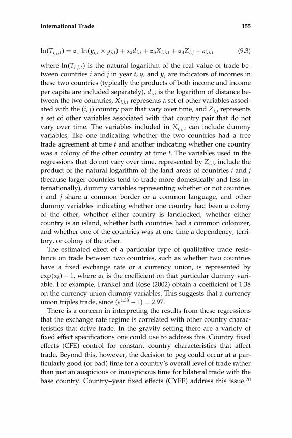
ln(Ti, j, t ) ¼ a1 ln(yi, t � yj, t)þ a2di, j þ a3Xi, j, t þ a4Zi, j þ e i, j, t (9.3)
where ln(Ti, j, t ) is the natural logarithm of the real value of trade be-
tween countries i and j in year t, yi and yj are indicators of incomes in
these two countries (typically the products of both income and income
per capita are included separately), di, j is the logarithm of distance be-
tween the two countries, Xi, j, t represents a set of other variables associ-
ated with the (i, j) country pair that vary over time, and Zi, j represents
a set of other variables associated with that country pair that do not
vary over time. The variables included in Xi, j, t can include dummy
variables, like one indicating whether the two countries had a free
trade agreement at time t and another indicating whether one country
was a colony of the other country at time t. The variables used in the
regressions that do not vary over time, represented by Zi, j, include the
product of the natural logarithm of the land areas of countries i and j
(because larger countries tend to trade more domestically and less in-
ternationally), dummy variables representing whether or not countries
i and j share a common border or a common language, and other
dummy variables indicating whether one country had been a colony
of the other, whether either country is landlocked, whether either
country is an island, whether both countries had a common colonizer,
and whether one of the countries was at one time a dependency, terri-
tory, or colony of the other.
The estimated effect of a particular type of qualitative trade resis-
tance on trade between two countries, such as whether two countries
have a fixed exchange rate or a currency union, is represented by
exp(ak)� 1, where ak is the coefficient on that particular dummy vari-
able. For example, Frankel and Rose (2002) obtain a coefficient of 1.38
on the currency union dummy variables. This suggests that a currency
union triples trade, since (e1:38 � 1) ¼ 2.97.
There is a concern in interpreting the results from these regressions
that the exchange rate regime is correlated with other country charac-
teristics that drive trade. In the gravity setting there are a variety of
fixed effect specifications one could use to address this. Country fixed
effects (CFE) control for constant country characteristics that affect
trade. Beyond this, however, the decision to peg could occur at a par-
ticularly good (or bad) time for a country’s overall level of trade rather
than just an auspicious or inauspicious time for bilateral trade with the
base country. Country–year fixed effects (CYFE) address this issue.20
International Trade 155

Finally, despite the wide range of other variables included in the
estimation of a gravity model, and CFE or even CYFE, there may be
omitted variables that affect bilateral trade and are correlated with a
fixed exchange rate. This can be addressed with the use of country-
pair fixed effects (CPFE) estimation where there is a separate dummy
for each country pair that exists.
CPFE estimation does not enable one to estimate the effects of any
variables that do not vary over the sample period, such as distance or
any variable denoted as Zi, j. Of course, the CPFE regressions control
for these factors, but their effects are subsumed in the dummy vari-
ables. This is of particular relevance when considering CPFE estimates
of the effects of fixed exchange rates on trade. Any country pair that
has a fixed exchange rate for the entire sample period will not yield in-
formation in the estimate of the impact of a fixed exchange rate on
trade. Rather, CPFE estimates identify the effect of fixed exchange rate
on trade only from those country pairs that switch exchange rate status
during the sample period. Thus the coefficient on the direct peg vari-
able in a CPFE regression represents the difference in trade due to a
fixed exchange rate between two countries that, at one time, had a
fixed exchange rate in place. But, as we have seen from chapter 4,
most fixed exchange rate regimes do not last for the entire sample, so
we lose information from relatively few country pairs when we use
CPFE estimation rather than CFE estimation. Of the 144 country pairs
that ever have a direct peg from 1973 to 1999, 118 change regime, with
56 of these switching once, 25 switching twice (i.e., both on and off a
peg), and 37 switching more than twice.
9.2.2 Estimates of the Effects of Fixed Exchange Rates on
International Trade
In this section we present estimates of the effects of fixed exchange
rates on trade.21 We build on the basic gravity model framework pre-
sented above, augmenting the specification with exchange rate regime
variables and indicators of exchange rate volatility that could poten-
tially affect trade resistance. The specification we use in this section is
ln(Ti, j, t ) ¼ a1 ln(yi, t � yj, t)þ a2di, j þ a3Xi, j, t þ a4Zi, j þ b1F1, i, j, t
þ b2F2, i, j, t þ b3CUi, j, t þ b4vi, j, t þ b5v2i, j, t þ e i, j, t (9.4)
where the variables that did not appear in the previous specification
include the direct peg dummy variable F1, i, j, t, the indirect peg dummy
156 Chapter 9

variable F2, i, j, t, the currency union dummy variable CUi, j, t, and the
indicators of exchange rate volatility, vi, j, t, and its square, v2i, j, t.
22
The direct peg fixed exchange rate dummy variable F1, i, j, t is based on
the Shambaugh (2004) classification system described in chapter 3. This
variable equals 1 for the (i, j) country pair in year t if there is a fixed ex-
change rate between country i and country j in that year (this means
one of these countries is a base). There are also indirect pegs, as repre-
sented by the dummy variable F2, i, j, t. These indirect pegs can be most
easily understood by comparing them to family relationships. For ex-
ample, two countries pegged to the same base will also be pegged to
one another in a ‘‘sibling’’ relationship (e.g., when India and South Af-
rica both were pegged to the US dollar). A ‘‘grandchild’’ indirect peg
occurs between a base country and another country pegged to a coun-
try that is itself pegged to the base (e.g., between Bhutan and the
United States when Bhutan pegged to the Indian rupee, which was it-
self pegged to the dollar). There can also be an indirect ‘‘aunt/uncle’’
relationship, such as that between Bhutan and South Africa, and the in-
direct ‘‘cousin’’ relationship, such as that between Bhutan and Lesotho,
whose currency was pegged to the South African rand. In our regres-
sions we include a separate indirect peg dummy variable that equals 1
for a country pair that has any of the family of indirect pegs described
here.
The currency union dummy variable CUi, j, t is the ‘‘strict’’ currency
union dummy variable developed by Rose. We include it separately,
rather than subsuming currency unions in the category of direct pegs,
to allow for the possibility that the effect of this type of fixed exchange
rate system on trade differs from the effect of other types of fixed ex-
change rates. Currency unions, direct pegs, and indirect pegs are all
mutually exclusive, and any one observation can only be coded as one
type of exchange rate regime.
The specification also includes the level and squared value of bilat-
eral nominal exchange rate variability between country i and country
j, vi, j, t and v2i, j, t. The inclusion of these variables allows us to consider
whether they affect trade while controlling for a fixed exchange rate,
and whether a fixed exchange rate significantly affects trade beyond
its effect on reducing exchange rate volatility. Fixed rates may have an
effect beyond that of reduced volatility for a number of reasons, most
notably, the greater certainty they afford with respect to the domestic
currency price paid at the time of a delivery when that payment
is made six months or more after a contract is signed. Even though
International Trade 157

currency pegs are impermanent, as shown in chapter 4, the results pre-
sented in that chapter also indicate that a forecast of a fixed exchange
rate is likely more reliable than a forecast of a continually quiescent
floating exchange rate. Thus a fixed rate could provide a degree of cer-
tainty that may be helpful in trading relationships.23
The data set used in this chapter is based on information on 181
countries over the period 1973 to 1999, yielding 4,381 country–year
observations (rather than 181� 27 ¼ 4,887 because some countries,
like Estonia, did not exist for the entire sample period). There are
11,805 separate country pairs (rather than (181� 180)/2 ¼ 16,290 be-
cause of missing observations), and over the 27 years of the sample
there are 168,868 observations. The sample includes 1,562 observations
with a direct peg. These direct peg relationships, while less than 1 per-
cent of the observations, account for 11 percent of average annual
world trade, since 90 percent of these pairs represent trade between a
base country, which is usually an industrial country, and a developing
country. The number of direct pegs in a bilateral trade data set will
necessarily be a small proportion of the number of overall observations
since any country can have a direct peg with only one other country
while it can trade with as many as 100 other countries. A more relevant
statistics therefore is that roughly half the country–year observations
are coded as pegs and 135 countries are involved in a peg at some
point, which is consistent with statistics presented in chapter 3. Any
direct peg can create a large number of indirect pegs, and there are
13,679 indirect peg observations. The 2,055 currency union observa-
tions, 88 percent of which are for pairs between two developing coun-
tries, includes all intertwining relationships within a multilateral
currency union (e.g., among the countries in the CFA), but not country
pairs in which two countries have both, unilaterally, adopted the cur-
rency of a third country (e.g., the pair of Panama and Liberia).24
Regression results are in table 9.1.25 The first column of this table
presents estimates with only year fixed effects and gravity controls.
The coefficient on direct pegs in this case is 0.58 and is statistically sig-
nificant at the 99 percent level of confidence. The regression result in
column 2 includes country fixed effects, and in this case the coefficient
on the direct peg variable, at 0.32, is about half as big as in column 1,
although it is still highly significant. The difference in these coefficients
in columns 1 and 2 reflects the way in which country fixed effects con-
trol for multilateral resistance. As mentioned above, it might be impor-
tant to allow these multilateral resistance terms to vary over time,
158 Chapter 9

Table 9.1
Core results
1 2 3 4OLS, time CFE, time CYFE CPFE, time
Direct peg 0.586** 0.324* 0.305* 0.194*(0.124) (0.145) (0.147) (0.089)
Indirect peg �0.351** �0.031 �0.071 �0.015(0.050) (0.040) (0.048) (0.028)
Currency union 1.341** 1.231** 1.159** 0.323**(0.158) (0.155) (0.156) (0.132)
Exchange rate volatility �0.262** �0.271** �0.143** �0.205**(0.046) (0.039) (0.053) (0.032)
(Exchange rate volatility)2 0.007** 0.007** 0.004** 0.006**(0.001) (0.001) (0.001) (0.001)
Ln(distance) �1.212** �1.431** �1.436**(0.025) (0.026) (0.026)
Ln(Real GDP) 0.968** 0.059 0.445**(0.010) (0.066) (0.061)
Ln(Real GDP per capita) 0.392** 0.322** 0.007(0.015) (0.063) (0.058)
Common language 0.342** 0.302** 0.302**(0.046) (0.050) (0.049)
Border 0.582** 0.360** 0.330**(0.126) (0.123) (0.123)
Regional Trade Agreement 1.050** 0.529** 0.533** 0.265**(0.139) (0.163) (0.168) (0.072)
Landlocked �0.250** �0.155(0.035) (0.322)
Island 0.007 2.168**(0.040) (0.228)
Ln(area) �0.106** 0.628**(0.009) (0.045)
Common colonizer 0.337** 0.547** 0.567**(0.073) (0.070) (0.069)
Current colony 0.741þ 0.104 �0.015 �0.032(0.383) (0.480) (0.374) (0.452)
Common country �0.511 0.472 0.556(0.877) (0.558) (0.507)
Colony 1.403** 1.398** 1.388**(0.120) (0.120) (0.120)
Observations 168,868 168,868 168,868 168,868
R2 0.64 0.71 0.73 0.87
Number of country pairs, FE 11,805
Impact of reducing volatilityfrom mean to zero
�1.5% �1.6% �0.8% �1.2%
Note: þ significant at 10% *significant at 5%; **at 1%. Standard errors are clustered atthe country-pair level and reported below coefficients; constant and fixed effects areincluded but not reported.Estimates for 1973–99. See Klein and Shambaugh (2006) for details.
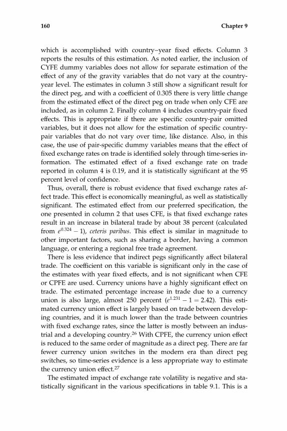
which is accomplished with country–year fixed effects. Column 3
reports the results of this estimation. As noted earlier, the inclusion of
CYFE dummy variables does not allow for separate estimation of the
effect of any of the gravity variables that do not vary at the country-
year level. The estimates in column 3 still show a significant result for
the direct peg, and with a coefficient of 0.305 there is very little change
from the estimated effect of the direct peg on trade when only CFE are
included, as in column 2. Finally column 4 includes country-pair fixed
effects. This is appropriate if there are specific country-pair omitted
variables, but it does not allow for the estimation of specific country-
pair variables that do not vary over time, like distance. Also, in this
case, the use of pair-specific dummy variables means that the effect of
fixed exchange rates on trade is identified solely through time-series in-
formation. The estimated effect of a fixed exchange rate on trade
reported in column 4 is 0.19, and it is statistically significant at the 95
percent level of confidence.
Thus, overall, there is robust evidence that fixed exchange rates af-
fect trade. This effect is economically meaningful, as well as statistically
significant. The estimated effect from our preferred specification, the
one presented in column 2 that uses CFE, is that fixed exchange rates
result in an increase in bilateral trade by about 38 percent (calculated
from e0:324 � 1), ceteris paribus. This effect is similar in magnitude to
other important factors, such as sharing a border, having a common
language, or entering a regional free trade agreement.
There is less evidence that indirect pegs significantly affect bilateral
trade. The coefficient on this variable is significant only in the case of
the estimates with year fixed effects, and is not significant when CFE
or CPFE are used. Currency unions have a highly significant effect on
trade. The estimated percentage increase in trade due to a currency
union is also large, almost 250 percent (e1:231 � 1 ¼ 2.42). This esti-
mated currency union effect is largely based on trade between develop-
ing countries, and it is much lower than the trade between countries
with fixed exchange rates, since the latter is mostly between an indus-
trial and a developing country.26 With CPFE, the currency union effect
is reduced to the same order of magnitude as a direct peg. There are far
fewer currency union switches in the modern era than direct peg
switches, so time-series evidence is a less appropriate way to estimate
the currency union effect.27
The estimated impact of exchange rate volatility is negative and sta-
tistically significant in the various specifications in table 9.1. This is a
160 Chapter 9

little surprising, given the general tenor of the results discussed in sec-
tion 9.1. But the economic relevance of this effect is relatively small.
The mean of volatility in this sample is 0.059, and therefore reducing
exchange rate volatility from this value to zero suggests only a 1 to 2
percent impact on trade. As mentioned above, this suggests that mea-
sured exchange rate volatility may not fully capture the increased cer-
tainty afforded by fixed exchange rates, even when controlling for
country-pair fixed effects that may be correlated with both the level of
trade and the choice of exchange rate regime.
We conclude this section by investigating the estimated effect of
fixed exchange rates on trade when using two of the other classifica-
tion systems presented in chapter 3; the IMF de jure classification based
on countries’ declared exchange rate status and the de facto classifica-
tion of Reinhart and Rogoff (2004). We collapse the multiple categories
in these classification schemes into either pegged or floating, as we did
in chapter 3. We might expect that coefficients on direct peg dummy
variables based on the IMF de jure scheme would be less significant
than coefficients presented in table 9.1, since, as discussed in chapter 3,
the de jure classification is misleading at times. It is not as clear a priori
what we might expect for the direct peg variable from the Reinhart–
Rogoff classification scheme as compared to what is presented in table
9.1. One might expect a less significant coefficient on the Reinhart–
Rogoff direct peg dummy than on the Shambaugh direct peg dummy,
since the latter captures the possible effect on trade of year-to-year in-
stability while this instability may not alter the pegged status of a
country in the Reinhart–Rogoff classification. On the other hand, we
might expect a more significant coefficient on the direct peg dummy
based on the Reinhart–Rogoff classification if their market-based ex-
change rates better capture the relevant exchange rate used in interna-
tional transactions than the official rate used by Shambaugh.
Table 9.2 shows the results using these two alternative classifications
with country year fixed effects included (i.e., it is comparable to the
results in column 3 of table 9.1). For purposes of comparison this table
also reports results using the Shambaugh classification but with the
smaller sample that is available when using the Reinhart–Rogoff classi-
fication. The results in this table show a strong similarity when using
either the Shambaugh or the Reinhart–Rogoff classification schemes.
The smaller data set has led to a slightly increased standard error for
the Shambaugh codes, pushing it past standard confidence intervals.
There is a bit more of a difference in the value of the coefficient on the
International Trade 161

indirect pegs, but the confidence intervals overlap at the 95 percent
level of significance. Thus, overall, the results are robust to using either
of these two de facto exchange rate classification schemes. In contrast,
results are weaker when using the IMF de jure classification. The esti-
mated effects of a de jure direct peg, reported in column 3 of table 9.2,
are both smaller than the respective results for either of the de facto
pegs, and the coefficients on the de jure direct pegs are not significant.
In many other chapters we have been concerned that omitted vari-
ables correlated with pegging could drive the results. As noted, our
fixed effect specifications were pursued with this in mind. In this case
Table 9.2
Results across different classifications
1 2 3Code RR JS IMF de jure
Direct peg 0.319* 0.264 0.146(0.157) (0.163) (0.176)
Indirect peg 0.112þ �0.070 �0.046(0.064) (0.055) (0.057)
Currency union 1.331** 1.298** 1.295**(0.178) (0.177) (0.178)
Exchange rate volatility �0.086 �0.091þ �0.091(0.055) (0.055) (0.055)
(exchange rate volatility)2 0.002 0.002 0.002(0.001) (0.001) (0.001)
Ln(distance) �1.308** �1.311** �1.311**(0.029) (0.029) (0.029)
Common language 0.340** 0.344** 0.345**(0.056) (0.056) (0.056)
Border 0.517** 0.512** 0.513**(0.135) (0.135) (0.135)
Regional Trade Agreement 0.068 0.081 0.080(0.185) (0.185) (0.185)
Common colony 0.625** 0.625** 0.624**(0.083) (0.083) (0.083)
Current colony �0.183 �0.172 �0.183(0.413) (0.424) (0.426)
Former Colony 1.244** 1.246** 1.266**(0.124) (0.124) (0.127)
Observations 123,393 123,393 123,276
R2 0.76 0.76 0.76
Note: þ significant at 10% *significant at 5%; ** significant at 1%.All columns include country year fixed effects. Constant not reported.Standard errors are clustered at the country–pair level and reported below coefficients.
162 Chapter 9

one may be even more concerned that these results reflect some reverse
causality; pegs might have begun in anticipation of an increase in
trade. While sound excludable instruments are difficult to find, Klein
and Shambaugh (2006) explore an instrumental variable estimation
using the exchange rate regime of neighboring countries as an instru-
ment. Results obtained with this method are very similar to those that
do not instrument for the peg variable.28
9.3 Conclusion
One of the presumed benefits of a fixed exchange rate is that it should
expand trade, at least with the base country. This has motivated calls
for fixed exchange rates in various parts of the world, and is a corner-
stone of OCA analysis as well (see chapter 2). Empirical backing for
this presumption, however, has proved elusive. This chapter shows
that when one focuses on bilateral exchange rate regimes as coded
from de facto performance, rather than using bilateral exchange rate
volatility as a proxy for regimes, there are statistically and economi-
cally significant impacts on trade from a fixed exchange rate. Thus,
while the previous chapter showed pegs contribute to a loss of mone-
tary autonomy for countries with open capital markets, this chapter
demonstrates that pegging promotes an expansion of bilateral trade
with the base country. Which of these effects is more important likely
depends on how important trade with the base country is to the econ-
omy, and how appropriate the base country’s monetary policy is for
the pegging country. Thus the general lessons from the trilemma and
OCA analysis discussed in chapter 2 have empirical support as a basis
for choosing an exchange rate regime. The next two chapters examine
more general aspects of macroeconomic performance across exchange
rate regimes, the behavior of inflation and economic growth across dif-
ferent regimes.
International Trade 163


10 Exchange Rate Regimes and Inflation
Inflation is always and everywhere a monetary phenomenon.
—Milton Friedman and Anna Schwartz, A Monetary History of the United States,1867–1960, 1963
Exchange rate regimes are monetary constructs. This is evident from
the policy trilemma, since monetary policy becomes subject to ex-
change rate management when a country has open capital markets.
Thus the famous dictum of Friedman and Schwartz that serves as the
epigraph of this chapter suggests that inflation would likely differ sys-
tematically between countries that peg and countries that do not peg
during the modern era.
The stark assertion by Friedman and Schwartz, of a monocausal
source of inflation, has another implication for the role of the pegged
exchange rates in determining inflation; there should be no effect of a
peg on inflation over and above the direct discipline it imposes on
monetary policy. Theoretical research on the credibility of monetary
policy, however, provides an additional channel by which the choice
of the exchange rate regime may affect inflation performance. This
theory suggests that the perception of the central bank’s policy prefer-
ences affects inflation performance. This credibility effect operates sep-
arately from actual monetary policy, although eventually there must
be a consistency between perceptions and reality.1 Empirical analysis
supports this theory, showing that central bank credibility affects infla-
tion.2 Thus we may expect a peg to contribute to lower inflation be-
yond its effect on disciplining monetary policy to the extent that it
bolsters the anti-inflation reputation of a central bank.
The credibility effects of the exchange rate regime on inflation are
likely to differ across time horizons. We might expect to find a stronger
credibility effect of a peg, over and above its discipline effect, at shorter

time horizons as compared to longer time horizons. Over a long hori-
zon, perceptions reflect actions. A central bank can sustain a ‘‘hawkish’’
reputation over time only if it persistently conducts policy in an anti-
inflationary manner. Thus, when looking at data representing average
values over a decade or two, actual monetary growth will fully capture
both the disciplinary and credibility effects of an exchange rate peg. In
this case inflation will appear as solely a monetary phenomenon, and
there will be no additional effect of a long-lived pegged exchange rate
regime on inflation other than its effect on money growth rates.3 An
analysis of annual data, however, may uncover a role for a pegged ex-
change rate to temper inflation beyond its direct effect on monetary
policy. Over this shorter horizon, expectations of future inflation may
respond to an exchange rate peg, and not just monetary growth that
year, since the peg is a highly visible and easily monitored monetary
commitment mechanism.4
In this chapter we investigate the links between the exchange rate
regime and inflation performance. We begin with a discussion that
frames the analysis. We then review the empirical literature on this
topic. This literature generally finds that the exchange rate regime sig-
nificantly affects inflation, even controlling for the influence of other
factors. In the third section we present our own estimates. These are
based on a data set representing the experience of 80 countries (22 in-
dustrial, and 58 nonindustrial) over the period 1980 to 1999. Using an-
nual data, we find evidence that a peg affects inflation through both
a disciplinary role and a credibility role. We also find that the peg
affects average inflation rates over this entire period by disciplining
monetary policy of nonindustrial countries, but it does not have a
similarly significant role for industrial countries. There is also no evi-
dence of a distinct credibility role for average inflation over these two
decades.
10.1 Exchange Rate Regimes and Inflation: A Basic Framework
The view of inflation as a monetary phenomenon suggests a model of
inflation based on money demand and money supply. We present a
heuristic approach to this problem in this section. We discuss the man-
ner in which an empirical specification can reflect both the disciplinary
and the credibility effects of an exchange rate peg. The appendix to this
chapter supports these specifications with a more formal approach
based on an explicit model.
166 Chapter 10

A very general specification of money demand for a time-series
cross-sectional data set takes the form
Mdi, t ¼ Pi, t � L(ii, t
(�)
,Yi, t(þ)
), (10.1)
where Mdi, t is the demand for money, Pi, t is the price level, Yi, t is real
income, and ii, t is the nominal interest rate, all for country i at time t.
The price level is included because the demand for money is a demand
for real balances, that is, (Mi, t/Pi, t). The liquidity demand function is
L(ii, t(�)
,Yi, t(þ)
), where the signs under the arguments represent their respec-
tive effects on the demand for money. Money demand increases with
real income because this variable serves as a proxy for the volume of
the desired transactions that require money. Money demand decreases
with an increase in the nominal interest rate, since this raises the op-
portunity cost of holding money rather than interest-bearing assets.
The nominal interest rate incorporates people’s views on expected in-
flation. This is shown by the Fisher equation,
ii, t ¼ ri, t þ p ei, t (10.2)
where ri, t is the real interest rate and p ei, t is the expected inflation rate.
The central bank supplies money to an economy. Equilibrium in the
money market requires that money demand equals money supply,
MSi, t. Since money demand and money supply are the equal in equilib-
rium, and since the money market, like other asset markets, clears vir-
tually moment-by-moment, we will denote both money demand and
money supply by Mi, t. Thus in equilibrium we have
Mi, t ¼ Pi, t � L(ri, t þ p ei, t
(�)
,Yi, t(þ)
) (10.3)
which can be rewritten as
Pi, t ¼ Mi, t/L(ri, t þ p ei, t
(�)
,Yi, t(þ)
). (10.4)
As shown in the appendix, this relationship can be expressed in per-
centage change terms. In this case inflation (the percentage change in
prices), pi, t, is a function of the percentage change in money supply,
the percentage change in income, and the expected inflation rate. Thus
a regression equation based on this relationship is
pi, t ¼ bEpei, t þ bM%DMi, t � bY%DYi, t þ e i, t, (10.5)
Inflation 167
where %DMi, t is the percentage change in the money supply, %DYi, t is
the growth of real national income, and e i, t is a regression error term.5
This specification can be modified to consider the effect of a pegged
exchange rate on inflation. A peg potentially affects two of the varia-
bles in (10.5): the contemporaneous growth of money %DMi, t through
its discipline effect; and expected future inflation rate p ei, t through its
credibility effect. We can jointly test for the discipline and credibility
roles of a peg by estimating
pi, t ¼ bPPEGi, t � bY%DYi, t þ e i, t. (10.6)
We expect that the estimate of bP < 0 because money growth is sys-
tematically lower in years in which a country pegs than in years in
which it does not, and for countries that persistently peg than for coun-
tries that do not.6 In addition to this discipline effect, the PEG dummy
variable in this specification also captures the credibility effect of fixing
the exchange rate on expectations of future inflation. This would bol-
ster the estimated negative value of bP since, with a persistent peg,
expected inflation will be lower in the future. As shown in (10.5), this
tempers inflation in the present.
An empirical specification that focuses only on a peg’s credibility ef-
fect is
pi, t ¼ bCP PEGi, t þ bM%DMi, t � bY%DYi, t þ e i, t. (10.7)
We expect bP < bCP < 0 because (10.7), unlike (10.6), controls for the
discipline effect of the peg through the inclusion of money growth as a
separate explanatory variable. The credibility effect of the peg operates
through its effect on expected future inflation, and therefore depends
on the likelihood of the persistence of the peg as well as the effect of
the peg on inflation. In the data we use in section 10.3, the probability
that a country maintains a peg from one year to the next is 90 percent,
a figure in line with the statistics presented in chapter 4. The credibility
effect also depends on the recognition that inflation is lower under a
peg than under a float. Table 10.1 (in section 10.3) demonstrates that
the average inflation rate when there is a peg is 56 percent of the aver-
age inflation rate when a currency floats in the sample used in this
chapter.
An alternative to estimating cross-sectional time-series regressions
with annual data is to estimate the effects of the exchange rate regime
on inflation for a long-horizon cross section. In section 10.3, along with
168 Chapter 10
regressions that use annual data for a cross section of countries, we
also present estimates of equations (10.6) and (10.7) where we use the
average value of the variables for countries over the period 1980 to
1999. A significant discipline effect of a peg that distinguishes it from a
float would lead to a negative coefficient on the peg variable in (10.6).
But, as discussed above, one would not expect a credibility effect of a
peg over and above its effect on monetary discipline in these cross-
sectional regressions, since expectations over twenty years should be
broadly consistent with actual behavior. Therefore we can reasonably
expect the long-run marginal credibility effect to be zero, even if we
find a significant credibility effect in the annual data.
The specifications presented in this section generally correspond to
ones used in empirical analyses of this topic. This discussion provides
a framework for interpreting results from the literature discussed in
the next section, as well as our own estimates that are presented in
section 10.3.
10.2 Empirical Studies of Exchange Rate Regimes on Inflation
There are two types of country-level empirical studies of the effects of
the exchange rate regime on inflation. One type considers particular
events in which the exchange rate serves a central role as a nominal an-
chor in a disinflationary strategy. These studies typically consider the
chronology of particular episodes, or the experience of a small set of
countries suffering from high inflation. For example, Collins (1988)
shows that the establishment of the European Monetary System in
1979 was not a significant contributing factor to the subsequent fall in
inflation rates among its members, despite claims made at that time,
and Vegh (1992) studies the role of exchange rate targets in efforts to
tame hyperinflations.7 A second type of empirical analysis focuses on
the systematic effects of the exchange rate regime on inflation across a
wider cross section of countries, which is the focus of the analysis in
this chapter. In this section we review existing research on this topic.8
Ghosh et al. (1997) conducted one of the first studies of the effects of
the exchange rate regime on inflation in a wide cross section of coun-
tries. Their analysis uses a tripartite classification system (‘‘pegs,’’ ‘‘in-
termediate,’’ and ‘‘float’’) and includes the experience of 140 countries
over the time period 1960 to 1990, using annual data. They document
differences in inflation under the three exchange rate arrangements.
They find that the average inflation rates were 8.4 percent in pegs, 11.6
Inflation 169
percent in intermediate regimes, and 15.2 percent in floating regimes,
although the pegs were predominantly in the 1960s when worldwide
inflation was lower.
Ghosh et al. also estimate the conditional effect of the exchange rate
regime on inflation.9 Their regressions include peg and intermediate
exchange rate dummy variables, the growth in real income, the change
in the nominal interest rate, an indicator of central bank turnover, and
an indicator of trade openness.10 Thus this specification is an aug-
mented version of equation (10.6), and the coefficients on the peg
dummy variables (analogous to bP) represent both credibility and dis-
cipline effects. Their estimates suggest that a peg lowers inflation by 5
percentage points as compared to a float (an estimate significant at
better than the 99 percent level of confidence), and an intermediate
exchange rate regime lowers inflation by 1.5 percentage points as
compared to a float (significant at better than the 90 percent level of
confidence). They also present regressions that include money growth
rates as well as the other regressors (so the coefficients on the peg
dummy variables are analogous to bCP in equation 10.7). The coeffi-
cients on the pegs are smaller (in absolute value) in these regressions
than in regressions that do not include money growth. The estimated
effect of a peg is the statistically significant reduction of inflation by 1.8
percentage points as compared to a float, while inflation performance
under an intermediate exchange rate regime is not statistically distin-
guishable from that under a float. Money growth is highly significant
in this regression. Thus these results suggest that a pegged exchange
rate affects annual inflation through both a disciplinary and a credibil-
ity role while an intermediate regime only affects inflation through the
direct discipline it imposes on monetary policy. The significant effect of
a peg on inflation is robust to other specifications, including a simulta-
neous equation model in which the decision by a country as to whether
or not to peg is jointly determined with the inflation rate.
Ghosh, Gulde, and Wolf followed up this working paper with a
chapter on the effects of the exchange rate regime on inflation in their
2002 book. They report similar results with respect to the effect of
pegged exchange rates and intermediate regimes on inflation. An im-
portant extension in this book is that they estimate the effect of ex-
change rate regimes on inflation for subsamples of the data. The effects
reported in their earlier working paper, that pegged exchange rates
lower inflation as compared to floats while intermediate regimes do
not, holds for upper middle-income countries. Both pegs and interme-
170 Chapter 10

diate regimes are associated with lower inflation than what occurs
with floating exchange rates for lower middle-income countries, while
neither have a significant effect for upper income countries.
Differences in the effects of the exchange rate regime on inflation
across income groups are also found by Levy-Yeyati and Sturzenegger
(2001). Their results are based on annual data, from 1974 to 1999, for
154 countries. Like the research by Ghosh et al., they also use a tripar-
tite exchange rate regime classification, although one drawn from their
own classification scheme (which is discussed in chapter 3). Their re-
gression estimates show a significant reduction in inflation if a country
pegs, conditional on a number of other factors including money
growth. Interestingly, the reported estimate is that pegs lower inflation
by 1.8 percentage points as compared to floats, the same point estimate
found by Ghosh et al. (1997). Also, as in Ghosh, Gulde, and Wolf
(2002), Levy-Yeyati and Sturzenegger find an effect of pegs on inflation
for low-volatility and nonindustrial countries but not for industrial
countries. Furthermore, by splitting the sample, Levy-Yeyati and Stur-
zenegger distinguish between pegs in place for five or more consecu-
tive years (‘‘long pegs’’) and those in place for less than this amount of
time (‘‘short pegs’’). They find that long pegs, but not short pegs, con-
tribute to lower inflation for nonindustrial countries.
Husain, Mody, and Rogoff (2005) also find differences in the effect of
the exchange rate regime on inflation across income groups. They use
yet another exchange rate classification, the Reinhart–Rogoff classifica-
tion (see chapter 3), in a data set with annual data for 158 countries
covering the period 1970 to 1999 (the data, but for the classification
scheme, is from Ghosh, Gulde, and Wolf 2002). In regressions that in-
clude money growth rates, as well as other regressors mentioned
above, they find a significant negative effect of pegging, as compared
to freely floating, only for emerging market and developing countries.
In addition, pegs delivered lower inflation than limited flexibility or
managed floating for developing (but not emerging market) countries.
Similarly Bleaney and Francisco (2007) report a significant negative ef-
fect of pegs on inflation in a time-series cross-section analysis that does
not include money growth as a regressor.
Alfaro (2005) uses annual data for 130 industrial and developing
countries over the period 1973 to 1998 to investigate whether inflation
is negatively related to openness, as proposed by Romer (1993). Romer
argued that the advantages of surprise inflation decrease with the
openness of an economy and, for that reason, inflation expectations,
Inflation 171

and inflation itself, are lower in open economies, all else equal.11 His
empirical tests using cross-country averages of inflation and openness
confirm this prediction. Alfaro also shows a negative relationship be-
tween inflation and openness in a cross-section of countries. But she
finds no relationship between openness and inflation in a time-series
cross section when she includes year and country dummy variables.
More to the point for this chapter, she finds that the exchange rate re-
gime is a statistically significant and economically relevant determi-
nant of inflation in the time-series cross-sectional data set. She uses
the IMF de jure classification scheme as well as a coding based on the
Reinhart–Rogoff de facto classification scheme. Estimates using either
scheme show a statistically significant reduction in inflation from
about 25 to 40 percent when a country has a peg as compared to when
it has a floating exchange rate, while controlling for other factors (but
not controlling for money growth).
The papers discussed in this section are relatively consistent in their
findings of a negative relationship in annual data between pegged ex-
change rates and inflation through the discipline effect, that is, when
monetary growth is not included as a regressor. There is less evidence
of an effect conditional on money growth, one that would reflect a
credibility channel over and above that provided by actual monetary
growth. In the next section we present our own results on this topic.
10.3 Evidence on Inflation and the Exchange Rate Regime
The discussion to this point suggests that the empirical link between
the exchange rate regime and inflation depends on the way the analy-
sis is framed. Inflation is likely to be lower when countries peg than at
other times, something that can be determined by estimating a simple
bivariate relationship using a peg dummy variable. Augmenting this
regression with other variables that affect inflation, other than the
growth of the money supply, offers estimates of the role of a peg on in-
flation through the discipline it imposes on monetary policy as well as
the credibility it confers concerning future policy. Adding the money
growth rate shows the role played by the peg through its effects on
credibility alone. In this section we present our own findings on the
role of the exchange rate regime on inflation for a cross section of coun-
tries using each of these approaches.
The main data set we use covers the experience of 80 countries over
the twenty-year period 1980 to 1999. Results are presented for the full
172 Chapter 10

set of 80 countries, as well as for the subset of the 22 richest countries
(labeled ‘‘Industrial countries’’ in the tables) and the 58 emerging-mar-
ket and developing countries (labeled ‘‘Developing countries’’).12
Most results for the set of developing countries exclude eleven coun-
tries that had an inflation rate above 100 percent for any year of the
sample (of course, none of the industrial countries had an inflation rate
this high during the sample period). This exclusion is an effort to limit
influence of outliers that would tilt estimates toward a significant tem-
pering of inflation by pegs. In one instance the significance of a peg dif-
fers depending on whether the results are based on the group of 58
developing countries that had no experience with very high inflation
or the wider set of 69 countries. In this case the table includes results
for both sets of developing countries. In all other cases, however, the
results concerning the significance of a peg on inflation are the same
across the 58-country and 69-country samples.13
The top panel of table 10.1 presents some basic statistics on inflation
in the 80-country data set and its subsets. The distribution of inflation
rates is skewed, as shown by the fact that the average inflation rate
(10.34 percent) is almost 45 percent bigger than the median rate (7.15
percent). Also, as might be expected, the average annual inflation rate
among developing countries is more than 80 percent larger than that
Table 10.1
Inflation statistics, 1980 to 1999
Inflation:average
Inflation:median
Obser-vations
Peg obser-vations (%) Countries
All countries 10.34% 7.15% 1,473 549 (37%) 80
Industrial countries 6.47% 4.02% 418 111 (27%) 22
Developing countries 11.87% 8.58% 1,055 438 (42%) 58
Pegs and inflation
Inflationi; t ¼ b0 þ bPEGPEGi; t þ ei; t
Allcountries
Industrialcountries
Developingcountries
b0 11.90* 7.59* 14.05*(1.13) (1.32) (1.44)
bPEG �4.20* �4.20* �5.25*(1.19) (1.35) (1.49)
Adjusted R2 0.032 0.055 0.045
Note: * significant at better than the 95% level of confidence.Standard errors are clustered at the country level and reported below coefficients.
Inflation 173

of industrial countries, while the median inflation rate for developing
countries is more than twice as big as that of industrial countries.
The lower panel of table 10.1 presents estimates of bivariate regres-
sions that use a dummy variable that equals 1 in years in which a
country pegs (the peg dummy is based on the Shambaugh classifica-
tion scheme described in chapter 3).14 Inflation is significantly lower in
years in which there is a peg as compared to other years. The average
inflation rate for all countries for years in which there is not a peg is
11.90 percent, while it is 7.70 percent when there is a peg. The effect of
a peg on reducing inflation is highly significant for both developing
and industrial countries.
These estimates, however, do not show the direct effects of a peg on
inflation since other factors may systematically differ with the presence
of a peg. Rather, we want a model-based analysis, like the specifica-
tions (10.6) and (10.7), to show how pegs contribute to tempering in-
flation. Table 10.2 offers an analysis of this type. The first three
columns of table 10.2 present estimates that do not include money
growth while the other four columns include the current and lagged
money growth rates. The regressions also include other variables that
potentially affect inflation. The growth in real GDP is expected to have
a negative effect on inflation, as shown in section 10.1. Also, as dis-
cussed in the literature review section, other variables have also been
used in panel regressions. Greater trade openness is expected to be
associated with lower inflation since the adverse consequences of infla-
tion are bigger for a more open economy, as pointed out by Romer
(1993). More openness with respect to capital flows, as well as trade
flows, is also theoretically associated with lower inflation, so the
expected effect of capital controls is to contribute to higher inflation.
Research has shown that leadership turnover at a country’s central
bank is associated with higher inflation. Finally adverse terms of trade
shocks can also contribute to inflation.
The results reported in the first three columns of table 10.2 show a
highly significant effect of pegs on inflation for the full set of countries,
as well as for the subsets of industrial countries and developing coun-
tries. Controlling for other factors, inflation is estimated to be lower by
4.35 percentage points in industrial countries and 4.16 percentage
points in developing countries (that had no experience with very high
inflation) in years in which there is a peg than in other years. This
could reflect both the discipline and credibility effects. The results in
columns 4 through 7 of table 10.2 reflect only the credibility effects
174 Chapter 10

Table
10.2
Inflationregressions,an
nual
data,
1980
to1999
Countrygroup
III
III
IVV
VI
VII
All
Industrial
Dev
elopinga
All
Industrial
Dev
eloping
Dev
elopinga
Peg
dummy
�3.70*
�4.35*
�4.16*
�1.29*
�2.27*
�1.26
�1.81*
(1.13)
(1.57)
(1.46)
(0.63)
(0.55)
(0.79)
(0.83)
%Dmoney
0.35*
0.24*
0.39
*0.56*
(0.05)
(0.10)
(0.05)
(0.05)
Lag
%Dmoney
0.26*
0.22*
0.26*
0.07
*(0.03)
(0.07)
(0.04)
(0.02)
%Dreal
GDP
�0.36*
�0.65*
�0.39*
�0.62*
�0.62*
�0.64*
�0.67*
(0.09)
(0.16)
(0.10)
(0.09)
(0.12)
(0.10)
(0.08)
Tradeopen
ness
�1.20
4.09
þ�3
.24þ
0.68
1.06
�0.70
�0.95
(1.30)
(2.30)
(1.70)
(0.86)
(1.22)
(1.06)
(1.03)
Cap
ital
controls
5.19
*7.44
*0.60
2.93*
4.21*
2.59
2.67þ
(1.50)
(1.93)
(2.69)
(0.91)
(1.17)
(1.44)
(1.39)
CBturnover
8.58
*�2
.71
8.24*
2.90þ
�3.63
3.57
*3.69
*(3.45)
(6.88)
(3.20)
(1.64)
(4.53)
(1.52)
(1.58)
%Dtotal
�0.11
0.67
0.36
�2.22
�6.38
�1.88
�3.43
(2.37)
(7.91)
(2.41)
(1.95)
(8.43)
(2.01)
(2.25)
Adjusted
R2
0.14
0.30
0.13
0.48
0.62
0.44
0.56
Observations
1,473
418
1,055
1,472
418
1,054
1,211
Note:*significantat
betterthan
the95%
level
ofconfiden
ce;þ
significantat
between90
%an
d95
%levelsofconfiden
ce.
a.Includes
countriesthat
experiencedhigh(>
100%
)inflation,thoughyears
withhighinflationareomitted.
Standarderrors
areclustered
atthecountrylevel
andreported
below
coefficien
ts.
Inflation 175

since money growth is included in these regressions. As predicted in
section 10.1, the coefficients on the peg dummy variable are smaller (in
absolute value) when the money growth variables are included in the
regression. The credibility effect is significant among industrial coun-
tries and, for these countries, about half of the effect of the peg on infla-
tion is through the credibility effect and half through the discipline
effect. There is no evidence of a significant credibility effect for the sub-
set of 58 developing countries. This differs from results from previous
research, as discussed in section 10.2, which tended to find significant
effects for a peg, while controlling for monetary growth, for developing
and emerging market countries but not for industrial countries. Part of
the reason for this is differences in the samples. To illustrate this point,
we present, in column 7, estimates that include the experience of the
eleven countries with experience of high inflation as well as the other
58 developing countries, although we omit observations for years in
which inflation exceeded 100 percent. Comparing the results in col-
umns 6 and 7 shows that these additional 157 observations cause the
coefficient on the peg variable to increase by over 40 percent. Also
this coefficient is significant at better than the 95 percent level of
confidence.15
The results in table 10.2, and indeed all estimates in this chapter, are
consistent with the basic model presented in section 10.1, since the
coefficients on the money growth variables and the growth of real
GDP are always significant at better than the 95 percent level of confi-
dence. The results for the full set of countries in table 10.2 show that an
increase in the rate of money growth by 10 percentage points, all else
equal, raises inflation by 3.5 percentage points that year and by 2.6 per-
centage points in the subsequent year. A one percentage point increase
in national income, all else equal, lowers inflation by 0.62 percentage
points. Capital controls are associated with significantly higher infla-
tion in industrial countries. There is also evidence that central bank
turnover is associated with higher inflation in developing countries.
One possible concern with these results is that the choice of whether
to peg could itself be a function of the inflation rate. If a country is
more likely to peg in years in which it has low inflation, then the coeffi-
cient on the peg dummy variable will overstate the effect of the peg on
inflation. But, in chapter 5, we showed that a country’s choice to peg its
currency tends to be associated with variables that, if they change at
all, tend to do so slowly. This would suggest that endogeneity might
not be a major concern. Nevertheless, to check for this possibility, we
176 Chapter 10

present instrumental variable (IV) estimates in the first three columns
of table 10.3. The top panel presents estimates that do not include
money growth while the bottom panel includes current and lagged
money growth. In each case, the two excluded instruments are dummy
variables showing whether a country pegged its currency continually
for the prior three years, and continually for the prior five years. The
coefficient on the three-year prior peg dummy variable is positive and
very significant in the first-stage of the instrumental variable estima-
tion and, as reported in the table, the adjusted R2 statistics on the first
stage are good. The pattern of the significance of results of the IV esti-
mates are the same as those of the OLS estimates presented in table
10.2; the peg dummy is significant at better than the 95 percent level of
confidence for the full sample, and both subsamples, when money
growth is excluded from the regression but is only significant at this
level of confidence for the industrial country sample when money
growth is included.16 Concerns about biased OLS results due to endo-
geneity are also allayed by the fact that the coefficients on the peg
dummy variable estimated with instrumental variables are uniformly
larger than those estimated with OLS.
Another potential concern is that countries that tend to peg also have
lower inflation for reasons unassociated with the peg that are not fully
captured through the inclusion of other variables in the regression.
One way to address this is to estimate the regressions using country
fixed effects (CFE). The coefficients in these estimates show the effect
on inflation that occurs when a country switches to a peg. These esti-
mates are presented in the columns 4 through 6 of table 10.3, with esti-
mated excluding money growth presented in the top panel and
estimates including money growth included in the bottom panel. In
this case, inflation is significantly lower only in the case of industrial
countries that switch to a peg, not for developing countries.17 This re-
sult for industrial countries is found for both the estimates that exclude
money growth and those that include money growth, so there is evi-
dence of significant credibility and discipline effects.18
The final sets of results, presented in table 10.4, correspond to the
specifications where we use a data set in which the dependent variable
is the average rate of inflation over the years 1980 to 1999, and the in-
dependent variables are the average rates of money growth, real GDP
growth, trade openness, capital controls, and central bank turnover
over this period. The peg indicator is a dummy variable that equals 1
if, during the twenty-year period, there was a continuous peg spell
Inflation 177

Table
10.3
Inflationregressions,an
nual
data,
1980
to1999:Alternativeestimationmethods
Disciplineandcredibilityeffects
Countrygroup
Countrygroup
All
Industrial
Dev
eloping
All
Industrial
Dev
eloping
IVEstim
ates
Estim
ates
withCFE
Peg
dummy
�4.83*
�5.37*
�5.88*
�3.08þ
�2.47*
�3.08
(1.49)
(2.04)
(1.88)
(1.70)
(0.79)
(2.22)
%Dreal
GDP
�0.36*
�0.65*
�0.38*
�0.32*
�0.90*
�0.28*
(0.09)
(0.16)
(0.10)
(0.10)
(0.22)
(0.10)
Tradeopen
ness
�0.86
4.85þ
�2.80
12.65*
18.85*
12.42*
(1.42)
(2.67)
(1.82)
(3.29)
(8.99)
(3.45)
Cap
ital
controls
5.18
*7.36*
0.61
4.42
*6.05*
2.86
(1.51)
(1.90)
(2.69)
(0.95)
(1.20)
(1.90)
Cen
tral
ban
kturnover
8.68
*�3
.03
8.46*
2.19
�10.55
5.42*
(3.41)
(6.98)
(3.10)
(3.78)
(13.27
)(2.47)
Adjusted
R2
0.14
0.30
0.13
0.45
0.46
0.43
IV:first-stag
ead
justed
R2
0.57
0.48
0.60
178 Chapter 10

Only
credibilityeffects
IVEstim
ates
Estim
ates
withCFE
Peg
dummy
�1.74þ
�4.09*
�1.52
�1.89
�1.81*
�1.93
(0.97)
(1.16)
(1.12)
(1.23)
(0.53)
(1.57)
%Dmoney
0.35
*0.23*
0.38
*0.26
*0.21*
0.28
*(0.05)
(0.10)
(0.05)
(0.05)
(0.10)
(0.05)
Lag
%Dmoney
0.26
*0.21*
0.27
*0.19
*0.20
*0.19
*(0.03)
(0.07)
(0.04)
(0.04)
(0.07)
(0.04)
%Dreal
GDP
�0.61*
�0.63*
�0.64*
�0.46*
�0.75*
�0.45*
(0.09)
(0.12)
(0.10)
(0.09)
(0.12)
(0.09)
Tradeopen
ness
�0.54
2.48þ
�0.64
6.99
*14
.06
6.60
*(0.92)
(1.37)
(1.10)
(2.35)
(8.25)
(2.36)
Cap
ital
controls
2.95
*4.17
*2.60þ
3.06
*3.66*
3.03þ
(0.92)
(1.15)
(1.44)
(0.92)
(1.60)
(1.68)
Cen
tral
ban
kturnover
3.00
þ�4
.20
3.65*
1.35
�7.26
3.41þ
(1.64)
(4.80)
(1.49)
(2.38)
(7.17)
(1.75)
Adjusted
R2
0.48
0.61
0.60
0.57
0.66
0.54
IV:first-stag
ead
justed
R2
0.58
0.50
0.44
Observations
1,472
418
1,054
1,472
418
1,054
Note:*Significantat
betterthan
the95%
level
ofconfiden
ce;þ
significantat
between90
%an
d95
%levelsofconfiden
ce.
Standarderrors
areclustered
atthecountrylevel
andreported
below
coefficien
ts.
Inflation 179

that lasted for at least ten years or two continuous peg spells that each
lasted for at least six years.19 As discussed in section 10.1, we expect a
significant and negative coefficient on the peg dummy variable when
average money growth is excluded from the specification if the peg
has an important discipline effect on monetary policy, and a coefficient
statistically indistinguishable from zero when average money growth
is included since any credibility effects should be captured in the mon-
etary growth variable.
Results in the first three columns of table 10.4 show that the coeffi-
cient on the peg variable is negative and significant in the regressions
that exclude money growth for the sample of 58 developing countries,
and for the full sample, but not for the sample of 22 industrial coun-
tries. Thus a peg seems to have a significant role in disciplining mone-
tary policy for developing countries, but not for industrial countries,
over this time horizon. This could be a reflection of the fact that, over
this period, there was a starker distinction between the monetary pol-
icy of developing countries that tended to peg and the monetary policy
of developing countries that did not tend to peg than that between in-
Table 10.4
Cross-country regressions, 1980 to 1999 average inflation rates
Country group
All IndustrialDevel-oping All Industrial
Devel-oping
Peg’s averagevalue
�3.50* �1.53 �3.65* 0.25 �0.70 0.80(1.44) (2.16) (1.75) (0.72) (0.94) (0.84)
%D money 0.88* 0.56* 1.00*(0.06) (0.10) (0.07)
%D real GDP �0.47 �0.49 �0.73 �1.38* �1.15* �1.43*(0.37) (0.82) (0.50) (0.28) (0.51) (0.26)
Trade openness �1.49 0.17 �4.12þ �0.06 �1.06 1.25(1.72) (2.68) (2.13) (0.87) (1.94) (0.91)
Capital controls 4.77* 5.89* �0.59 2.48* 3.84* 3.94*(2.05) (2.07) (3.25) (0.89) (1.17) (1.17)
Central bankturnover
16.24* 26.13* 10.45 1.16 4.35 1.77(7.10) (10.10) (6.43) (2.45) (6.51) (2.86)
Adjusted R2 0.32 0.73 0.33 0.86 0.90 0.87
Observations 80 22 58 80 22 58
Note: * significant at better than the 95% level of confidence; þ significant at between90% and 95% levels of confidence.Standard errors are robust to heteroskedasticity and reported below coefficients.
180 Chapter 10
dustrial countries that tended to peg and the other industrial countries.
Pegging may have been an effective disciplinary device for developing
countries, but industrial countries did not need to peg in order to con-
duct monetary policy in a disciplined fashion.
The importance of monetary growth for inflation is shown in col-
umns 4, 5, and 6 of table 10.4. In each of these columns the coefficients
on the average money growth and average GDP growth are of the
expected signs and highly significant (note the change in the signifi-
cance of the coefficient on average GDP growth when money growth
is included as a regressor). The R2 statistics in these columns indicate
that these models do a very good job of explaining the cross-country
variation in inflation. But, as predicted in section 10.1, whether a coun-
try pegs is not a significant part of this explanation, once money
growth is included in the regression. The point estimates of the coeffi-
cients on the peg indicator are small and insignificant when average
money growth is included. These results seem to suggest that average
inflation over two decades is, in fact, a monetary phenomenon.
10.4 Conclusion
The discussion of the policy trilemma in chapters 2 and 9, along with a
framework in which prices reflect monetary developments, suggests
an important role for the exchange rate regime in influencing inflation.
In this chapter we have shown that inflation is significantly lower
when countries peg than when they float. There are at least two possi-
ble reasons for this, one linked to the discipline a peg imposes on mon-
etary policy and another corresponding to the manner in which a peg
affects expectations over and above its direct influence on monetary
policy. There is evidence for both of these channels being important, at
least in annual data. There is also evidence of the role of a peg in disci-
plining monetary policy of developing countries over longer horizons,
but it is less clear that a peg offers a discipline to central banks of in-
dustrial countries that they would not otherwise exhibit.
These results suggest that pegged exchange rates can help discipline
policy in a way that can temper inflation. Previous chapters have
shown that pegged exchange rates can help foster bilateral trade but
generate a loss of monetary autonomy. Are there more consequences
for other economic outcomes, like economic growth, that add to the
cost–benefit calculus of exchange rate regime choice? We turn to that
topic in the next chapter.
Inflation 181

Appendix
The ideas presented in section 10.1 can be motivated through an analy-
sis based on the classic Cagan (1956) money demand function. This
function takes the form
Mdt
Pt¼ Ya
t e�lit , (10A.1)
where Mdt is the demand for money, Pt is the price level, Yt is real in-
come, and it is the nominal interest rate, all at time t. Equilibrium in
the money market requires that money demand equals money supply.
We assume that the effective money supply at time t, MSt , is a function
of a broad monetary aggregate, Mt, and a random element, Vt, such
that20
MSt ¼ Mte
Vt .
Another important component in this analysis, one discussed in sec-
tion 10.1, is the Fisher equation:
it ¼ rt þ pet ,
where rt is the real interest rate and pet is the expected inflation rate,
which we defined as
pet ¼ ln(Pe
tþ1)� ln(Pt).
Setting money supply equal to money demand, taking the natural log-
arithm of this equilibrium equation, using the Fisher equation, and rep-
resenting the logarithm all variables other than interest rates by
lowercase letters (so ln(Xt ) ¼ xt), we have
mt þ vt � pt ¼ ayt � l(petþ1 � pt).
Subtracting this equation from its one-period lead, and defining Dxt ¼xtþ1 � xt, we obtain, after some rearranging,
pt ¼ l
1þ lpetþ1 þ
1
1þ lDm� a
1þ lDyt þ et, (10A.2)
where we have defined the regression error term as the sum of the
unobservable change in the real interest rate and the change in the
money supply shock, that is,
182 Chapter 10

et ¼ l
1þ lDrt þ 1
1þ lDvt.
This equation serves as the basic framework for an analysis of the effect
of the exchange rate regime on inflation, once we also specify a link be-
tween the exchange rate regime and inflation expectations.
Under the assumption of long-run monetary neutrality, the long-run
proportional change in the price level equals the long-run proportional
change in the money supply, that is,
p ¼ Dm.
Furthermore, with purchasing power parity (PPP), the proportional
change in the exchange rate is the difference in the rates of money
growth between the home country and the foreign country, that is,
De ¼ Dm� Dm*.
An implication of this equation is that the expected long-run inflation
rate of a country with a credible peg is the expected long-run inflation
rate of its base country. If this inflation is less than the expected long-
run inflation rate that the country would otherwise have, then
expected adherence to the peg tempers inflation expectations, which,
as shown by (10A.2), lowers current inflation. This effect may be pres-
ent even when controlling for money growth over a short time hori-
zon. Over a longer horizon, however, a peg only operates through its
effect on actual monetary growth if expectations of monetary policy
are, on average, consistent with actual monetary policy.
Inflation 183


11 Exchange Rate Regimes and Economic Growth
Everything reminds Milton Friedman of the money supply. Well, everythingreminds me of sex, but I keep it out of the paper.
—Robert Solow
Long-run monetary neutrality is one of the oldest, and most widely
accepted, propositions in macroeconomics. One implication of this
proposition is that the long-run real value of an economy’s output can-
not be altered simply by printing money. More broadly, long-run mon-
etary neutrality implies that no nominal variable has an effect on real
outcomes over an extended period of time (though there is debate on
the time frame over which this proposition holds).1
A corollary of long-run monetary neutrality, one of interest for the
topic of this book, is of the long-run neutrality of the choice of the ex-
change rate regime. In particular, monetary neutrality implies that the
choice of an exchange rate regime has no impact on long-run economic
growth. Given the widespread acceptance of monetary neutrality, one
can take this as the baseline view on the topic of the effect of exchange
rate regime on long-run economic growth.
Arguments are made, however, that the exchange rate is a particu-
larly important price, and efforts to manage it might have long-run
consequences.2 The channels by which this operates could be through
effects discussed in earlier chapters of this book. Those chapters dem-
onstrate aggregate and macroeconomic consequences of the choice of
the exchange rate regime, albeit at shorter time horizons than those
usually considered in discussions of long-run growth: a link between
real exchange rate volatility and the nominal exchange rate regime is
discussed in chapters 6 and 7; the implication of the exchange rate re-
gime for the conduct of monetary policy is the central theme of chapter
8; evidence presented in chapter 9 shows that fixed exchange rates pro-
mote bilateral trade; and the previous chapter discusses the role of the
exchange rate regime in long-run inflation performance. Real exchange
rate volatility, macroeconomic stability, trade, and inflation are poten-
tial determinants of long-run economic performance. Therefore there
are potential roles for the exchange rate regime to influence long-run
economic growth through its effect on these variables. In addition there
may be other channels as well, such as the effect of the exchange rate
regime on the volatility of the terms of trade, on the persistence of the
overvaluation or the undervaluation of the exchange rate, on financial
development, and on the frequency and severity of financial crises.
Ultimately, the question of the effect of the exchange rate regime on
long-run economic growth is judged by empirics rather than theory. In
this chapter we address this question. We begin, in section 11.1, with a
discussion of the potential roles that the exchange rate regime can have
on growth. This section also includes a survey of the literature on this
topic. In section 11.2 we present an empirical analysis of the effects of
the exchange rate regime on long-run economic growth using a stan-
dard cross-country growth regression framework. This framework is
informed by one of the central themes of this book, the impermanence
of the exchange rate regime for many countries. The results presented
in chapter 4 show that while some countries maintain a peg or a float-
ing regime for an extended period of time, others flip from one type of
regime to another. Therefore, to capture this behavior, in our empirical
analysis we distinguish between countries that tend to peg their cur-
rency, countries that tend to allow their currency to float, and countries
that tend to flip from one type of regime to another over the relevant
period.
The basic result, of both the majority of papers surveyed and our
own empirical analysis presented in this chapter, is that there is little
evidence of the exchange rate regime per se on long-run economic
growth once one controls for other variables that typically are included
in growth regressions. This conclusion depends, to some extent, by
what is meant by the long run. Analysis of long-run economic growth
typically considers experience over a minimum of a decade, and, more
often, over the course of two or more decades. We find little evidence
of a role for the exchange rate regime on growth over twenty years,
but some evidence for its effects over the course of a decade, or a five-
year horizon. We also find the effect of the exchange rate regime on
growth depends on whether one is considering the richest industrial
186 Chapter 11

countries or a set of developing and emerging market countries. There
is stronger evidence of an effect in the latter group than in the former.
Thus our basic conclusion concerning the effect of the exchange rate on
twenty-year growth agrees with Ghosh, Gulde, and Wolf (2002) who
write ‘‘Overall, and in line with the theoretical literature, the results do
not suggest a strong link between the exchange rate regime and real
GDP growth’’ (p. 98). We find more support for the contention that
pegged exchange rates are associated with slower growth in develop-
ing and emerging market countries over shorter horizons.
11.1 Theories and Evidence on the Exchange Rate Regime and
Growth
At the outset of the modern era, certain economic implications of ex-
change rate regimes were quickly evident; for example, it was soon
clear that flexible rates were more volatile than what was predicted by
simple monetary models. At that early stage, however, it was difficult
to attribute differences in economic performance to a change in the pre-
vailing exchange rate regime. The decade of the 1970s was marked by
a number of factors, such as high energy and food prices and monetary
instability, which distinguished it from earlier postwar decades. It was
not until the end of the 1980s that the first empirical efforts to consider
the differences of long-run economic performance across a wide cross
section of countries that were attributable to exchange rate regimes
were published. In an influential work, Baxter and Stockman (1989)
showed that real exchange rate volatility differed in fixed and flexible
exchange rate regimes, but growth of GDP and consumption were sta-
tistically similar in both regimes.
A few years after the publication of Baxter and Stockman’s work,
Summers and Heston published The Penn World Table, a data set pro-
viding data on income, growth, investment, and other macroeconomic
variables for a wide set of countries (Summers and Heston 1991). These
data enabled researchers to run cross-country growth regressions, and
many quickly took advantage of this opportunity. A focus of the first
papers in this area was to test for convergence, that poor countries
grow faster than rich ones, and for conditional convergence, that con-
vergence occurred once one controlled for other factors suggested by
the Solow (1956) growth model, such as population growth and initial
investment (which was taken as a proxy for the savings rate). Influen-
tial papers that presented some of the first evidence for conditional
Economic Growth 187
convergence include Barro (1991) and Mankiw, Romer, and Weil
(1992).
The cross-country empirical growth framework then became very
popular for analyzing the effects of a wide range of political, economic,
and social variables on the long-run performance of economies. The
Solow model suggests that any factor that affects the long-run steady
state level of income per capita of an economy can be used as a regres-
sor in a properly specified growth equation. A positive and significant
coefficient on one of these variables suggests that it contributes to
higher levels of long-run growth, conditional on the other variables
included in the regression.3
Analyses of the effect of the exchange rate regime on growth typi-
cally take this tack, and go beyond simple correlations between the ex-
change rate regime and growth performance to the augmentation of a
standard growth regression with an indicator of the exchange rate re-
gime. An important contribution along these lines is by Levy-Yeyati
and Sturzenegger (2003). They use the exchange rate classification sys-
tem they developed (see chapter 3) to generate regressors representing
fixed exchange rate regimes, intermediate regimes, and floating ex-
change rate regimes. Their main regressions include annual data from
1974 to 2000 for 183 countries (though not all countries have observa-
tions for all years). Thus these regressions are not testing long-run
growth performance per se, rather annual growth over 26 years for a
panel of countries. They present evidence that countries that have a
floating exchange rate in a particular year grow significantly faster
than countries with less flexible regimes, with an estimated difference
of 0.78 percent per year (their table 5, column ii). They point out that
this is due to the performance on nonindustrial countries. In this sub-
set, the estimated significant difference in economic growth between
countries that have a floating exchange rate in a particular year and
countries that do not is over 1 percent (their table 5, column iv). They
also present cross-sectional analyses for the 1974 to 1999 period in
which the dependent variable for a single observation represents the
average rate of growth of a country over these twenty-five-years. The
independent variable representing the exchange rate regime is either
the percentage of years that a country had a fixed exchange rate during
this period, or the average of the LYS classification index for a country
during this period. As with the regressions utilizing annual data, they
find that greater exchange rate flexibility is associated with signifi-
cantly higher growth rates, especially for nonindustrial countries.
188 Chapter 11

While they conclude with some suggestions for reasons behind these
results, they also write: ‘‘As it stands, the paper opens more questions
than it answers. If we accept the results reported here, one can only
wonder why countries have opted so pervasively for unilateral pegs’’
(p. 1188).
There are reasons that policy makers, especially in nonindustrial
countries, may opt for pegged exchange rates, notwithstanding the
Levy-Yeyati and Sturzenegger results.4 Fixed exchange rates are asso-
ciated with higher bilateral trade (as shown in chapter 10). Increased
trade is associated with faster economic growth (Frankel and Romer
1999; Feyrer 2008). However, the growth effect concerns multilateral
trade while the exchange rate peg only affects bilateral trade flows
with the base country, and with other countries that peg to the same
base. There is also the Baxter and Stockman (1989) evidence that real
exchange rates are more stable when a country operates with a peg
than when it allows its currency to float, as well as more recent evi-
dence that shows a similar result for the terms of trade (Broda 2001). A
fixed exchange rate may also be one way in which a country obtains a
persistently undervalued real exchange rate which can be a vehicle for
promoting export-led growth (Mundell 2000; Rodrik 2008). Macro-
economic stability, especially low inflation that accompanies a strongly
pegged exchange rate, can also contribute to growth by promoting the
development of a country’s financial sector (Dornbusch 2001).
Alternatively, the Levy-Yeyati and Sturzenegger (2003) result, that
for nonindustrial countries flexible exchange rates are associated with
better growth performance, is consistent with analyses that focus on
the potential instability associated with pegged exchange rates. Calvo
(1999) argues that investment can be diminished, and therefore long-
run growth adversely affected, in a country with a pegged exchange
rate because interest rates rise due to both the uncertainty associated
with potential collapse of a peg and the defense of a peg under attack.
The evidence of a link between exchange rate crises and banking crises
(Kaminsky and Reinhart 1999), and the large adverse consequences of
banking crises on growth, also points to a potential reason why Levy-
Yeyati and Sturzenegger found greater exchange rate flexibility associ-
ated with better growth performance in nonindustrial countries.
But just as theory does not point unambiguously toward the role of
exchange rate regimes on growth, empirical work also offers mixed
results. Miles (2006) augments the Levy-Yeyati and Sturzenegger
regressions for nonindustrial countries with an additional regressor,
Economic Growth 189
the black market premium, which represents distortions in the econ-
omy. He finds that a fixed exchange rate regime has no independent
effect on growth but may exacerbate existing distortions and, in so
doing, adversely affect growth. Ghosh, Gulde, and Wolf (2002) find
some evidence that basket pegs and various intermediate regimes are
associated with higher growth rates than either flexible exchange rate
regimes or pegged exchange rate regimes, when controlling for other
factors that are typically considered determinants of economic growth.
Nevertheless, their overall conclusion, cited in the introduction of this
chapter, is one where they eschew a ‘‘strong link’’ between the ex-
change rate regime and economic growth.
The Levy-Yeyati and Sturzenegger result is somewhat supported
by two papers written by Bailliu, Lafrance, and Perrault, although in
each case there is a caveat. In their 2000 paper, employing a panel of
twenty-five emerging-market countries over the 1973 to 1998 period,
they find that flexible exchange rates are associated with higher eco-
nomic growth for emerging market countries if those countries are
open to international capital flows. In their 2003 paper, they use a
larger panel of sixty countries over a shorter time period of 1973 to
1988 and presents evidence that more flexible exchange rate regimes
are associated with faster growth if the country also has a monetary
anchor, but slower growth if the country does not.
Husain, Mody, and Rogoff (2005) also find that floating exchange
rates are associated with faster growth, but only for richer economies.
Using the Reinhart–Rogoff classification scheme, they find that the cat-
egory of floating exchange rates is not significantly associated with
faster growth for emerging market and developing countries, and the
category of ‘‘freely falling’’ is associated with lower growth. This con-
trasts with the Levy-Yeyati and Sturzenegger result as regards the ef-
fect of exchange rate volatility on growth for nonindustrial economies.
Husain, Mody, and Rogoff attribute the difference in their results to
those of Levy-Yeyati and Sturzenegger to the fact that ‘‘Several missing
and inconclusive observations in the Levy-Yeyati and Sturzenegger
(2003) classification raise concern about their conclusions’’ (p. 60, n.21).
But Bleaney and Francisco (2007) find that results using the Reinhart–
Rogoff classification scheme differ from those using four other classifi-
cations (three discussed in chapter 3, IMF de jure, LYS, Shambaugh,
and additionally one developed by Bubula and Otker-Robe 2002).
They present evidence that the Reinhart–Rogoff classification scheme
yields much worse outcomes for floating than any other classification.
190 Chapter 11

They attribute this result to ‘‘some unanticipated biases in the RR’s
float classification, which may be exacerbated by its relative rarity’’ (p.
12), which ‘‘raise some questions about its reliability’’ (p. 14). Bleaney
and Francisco conclude that hard pegs are associated with slower
growth, floating is not linked to faster growth (in contrast to LYS), and
that four of the five classification schemes show that growth rates in
developing countries are similar under soft pegs and floats. Their esti-
mates that use the Reinhart–Rogoff classification differ markedly from
the ones they present that use other classification schemes.
We summarize the research discussed here in table 11.1. As shown
in this table, and as discussed above, the contrasting results in this line
of research do not point toward a single interpretation of the evidence.
Therefore we offer our own empirical analysis in the next section.
11.2 Exchange Rate Regimes and Growth: An Empirical Analysis
In this section we present our empirical analysis of the effects of ex-
change rate regimes on economic growth. The sample includes 92
countries over the period 1980 to 1999. The analysis addresses a num-
ber of issues raised in our discussion above. We present results both
for the full sample of countries and for the two subsamples (22 indus-
trial countries and 70 nonindustrial countries), since previous research
shows cases of important differences between industrial and nonindus-
trial countries. To address the issue of the relevant time frame for the
analysis, we present three sets of regressions: a twenty-year panel with
one observation per country; a panel with two decade-long nonover-
lapping observations per country; and a panel with four observations
for each country, each one representing a nonoverlapping five-year
period.
The central variables of interest in these regressions are the indica-
tors of exchange rate regime. For each time frame we have three cate-
gories of exchange rate regime: peggers, floaters, and flippers. We do
not simply look at average time pegging because consistently pegging
differs from flipping. The general rule we employ is that a country is
classified as a pegger if it was in either one peg spell, or cumulatively
in two peg spells, for at least 75 percent of the sample period. For ex-
ample, in the twenty-year panel, a country is categorized as a pegger
if it has a peg spell of at least fifteen years, or if its two longest con-
tinuous peg spells combined are at least fifteen years (this is based on
the Shambaugh exchange rate classification discussed in chapter 3).
Economic Growth 191

Table 11.1
Survey of literature
Publication Countries
Sample andobservationhorizon
Exchangerate classifi-cation Results
Levy–Yeyati andSturzenegger,AER, 2003
183 (annual) or88 (x-section)(with 73nonindustrial)
1974–2000 forannual analysis;1974–1999 forx-section; 1976–2000 for 5-yearaverage
LYS, 3categories(annual) or %years fixed orLYS average(x-section)
No effect forindustrialcountries; floatsignificant (þ) fornonindustrial;peg significant(�) x-section
Miles, JED,2006
72 developingcountries(includingLuxembourg,South Africa)
1976–2000 forannual analysis;1975–2000 for5-year average;1975–2000 forx-section
LYS average,3 categories(float,intermediate,peg)
Fix has (�) sig.effect in 5-year(include blackmarketpremium); notindependentlysignificant inannual or inx-section
Bailliu,Lafrance, andPerrault 2000
25 emergingmarketcountries
1973–1998 for5-year average
IMF de jure
and HMR 2-step system(3 categories)
Change in ERRsignificance (�);flexible hasfaster growth incountries withmore opencapital markets
Bailliu,Lafrance,and Perrault,International
Finance, 2003
60 developingand industrialcountries
1973–1998 for5-year average
IMF de jureand HMR 2-step system(3 categories)
Intermediate andflex faster, butonly if withmonetary anchor
Ghosh, Gulde,and Wolfe2002
158 countries 1970–1995 IMF de jureand‘‘consensus’’
Peg, intermediatesignificance (þ),more so forlower and lowermiddle incomecountries
Husain, Mody,and Rogoff,JME, 2005
158 countries:32 advanced,25 emerging,103 developing
1970–1999annual data
IMF de jure
andReinhart–Rogoff
More flexibleweakly þ inadvancedcountries
192 Chapter 11
Likewise a country is categorized as a floater if it has a float spell of at
least fifteen years, or if the sum of its two longest continuous float
spells is at least fifteen years. A country that is neither a floater not
a pegger is categorized as a flipper. There are comparable rules for
the ten-year panel and the five-year panel. The peg and float dummy
variables equals 1 in the ten-year panel if a country had a peg or a
float, respectively, of at least eight years, or its two longest continuous
pegs or floats, respectively, are at least eight years. In the five-year
panel, an observation requires four years of a peg or a float, either in
one or two continuous spells, in order to be categorized as a peg or a
float, respectively.5
Table 11.2 presents the number of observations counted as pegged
or floating in the twenty-year panel, the ten-year panel, and the five-
year panel. There are proportionately fewer flippers as we move from
the twenty-year panel (in which there are 33 of the 92 countries) to the
ten-year panel (in which there are 41 out of the 184 observations) to the
five-year panel (with 51 flippers out of the 368 observations). The
lower panels of table 11.2 include results based on the subsets of indus-
trial countries and nonindustrial (i.e., developing and emerging mar-
ket) countries. These lower panels show that the proportion of flippers
drops off dramatically for the nonindustrial countries, from 28 of 70 in
the twenty-year panel, to 30 of 140 in the ten-year panel, and to 36 of
280 in the five-year panel. This proportionate change is smaller for the
industrial countries, with the number of flippers changing from 5 of 22
in the twenty-year panel, to 11 of 44 in the ten-year panel, and to 15 of
88 in the five-year panel. Thus, as we move to longer horizons, the
countries counted as peggers or flippers will change. Also the differ-
ence in results at twenty-year and five-year horizons may not simply
be the different effects of an exchange rate regime at different horizons,
but may also come from the fact that pegging for twenty straight years
is very different from pegging for five straight years.
Table 11.2 also includes results for the simple regressions
Growthi, t ¼ b0 þ bPEGPEGþ bFLIPFLIPþ e i, t (11.1)
where Growthi, t is the average annual rate of real per capita income
growth for country i over time period t, with t ¼ 1980–1999 for the
twenty-year panel, t ¼ 1980–1989 and 1990–1999 for the ten-year panel,
and t ¼ 1980–1984, 1985–1989, 1990–1994, and 1995–1999 for the five-
year panel. The results in the table include values of the coefficients bPEGand bFLIP, which tests for the difference between pegs and floats and
Economic Growth 193

Table 11.2
Regressions with only exchange rate regime dummy variables
Sample and itscharacteristics Coefficient 20 year 10 year 5 year
PEG (vs. FLOAT) �0.010þ �0.012* �0.011*(0.0056) (0.004) (0.004)
FLIP (vs. FLOAT) �0.000 0.012* 0.009*(0.004) (0.004) (0.005)
Full sample: 92countries, averageannual growth of1.19%
PEG� FLIP �0.010þ �0.024* �0.020*(0.006) (0.004) (0.005)
Adjusted R2 0.05 0.14 0.05
Observations with PEG ¼ 1 / Total 18 / 92 49 / 184 112 / 368
FLOAT ¼ 1 / Total 41 / 92 94 / 184 205 / 368
FLIP ¼ 1 / Total 33 / 92 41 / 184 51 / 368
PEG (vs. FLOAT) 0.008 0.007 0.008*(0.007) (0.004) (0.004)
FLIP (vs. FLOAT) 0.004 0.004 0.008(0.005) (0.004) (0.006)
Industrial countrysample: 22 countries,average annualgrowth of 2.11%
PEG� FLIP 0.004 0.003 0.000(0.008) (0.006) (0.006)
Adjusted R2 0.14 0.07 0.06
Observations with PEG ¼ 1 / Total 3 / 22 7 / 44 20 / 88
FLOAT ¼ 1 / Total 14 / 22 26 / 44 53 / 88
FLIP ¼ 1 / Total 5 / 22 11 / 44 15 / 88
PEG (vs. FLOAT) �0.012* �0.014* �0.015*(0.006) (0.004) (0.004)
FLIP (vs. FLOAT) 0.001 0.015* 0.009(0.005) (0.005) (0.006)
Nonindustrial countrysample: 70 countries,average annualgrowth of 0.90%
PEG� FLIP �0.013* �0.029* �0.024*(0.006) (0.005) (0.007)
Adjusted R2 0.07 0.18 0.07
Observations with PEG ¼ 1 / Total 15 / 70 42 / 140 92 / 280
FLOAT ¼ 1 / Total 27 / 70 68 / 140 152 / 280
FLIP ¼ 1 / Total 28 / 70 30 / 140 36 / 280
Note: * represents significant at 95% level of confidence or better; þ represent significantat 90% to 95% levels of confidence. Standard errors are corrected for heteroskedasticity(robust standard errors) and reported below coefficients. Sample: 1980–2000.
194 Chapter 11

flips and floats respectively, as well as results from performing the test
bPEG � bFLIP, which tests for the difference between pegs and flips.
Results for the pooled sample of industrial and nonindustrial coun-
tries, presented in the top panel of table 11.2, show that growth is
lower during periods that countries tend to peg than during periods
that countries tend to float or during periods that countries flip ex-
change rate regimes. These differences are only significant at between
the 90 percent and 95 percent level of confidence for the twenty-year
panel, but at better than the 95 percent level of confidence for both the
ten-year and five-year panels. The results in the lower two panels of
this table, however, caution us that we should consider the experiences
of the 22 industrial countries separately from that of the 70 nonindus-
trial countries. The only significant result for the industrial countries is
faster growth for countries during five-year periods when they peg as
compared to when they float. Nonindustrial countries, however, show
significantly slower growth when pegging as compared to both float-
ing or flipping across all three time horizons. These results are econom-
ically meaningful as well as statistically significant. For example, the
average growth rate for nonindustrial countries was 0.9 percent per
year over the sample period. Coefficients in the twenty-year panel of
�0.012 and �0.013 show that there was an economically meaningful
difference, not just a statistically significant difference, in the experience
of peggers versus floaters, and peggers versus flippers respectively.
This basic correlation of peg status and growth does not represent a
properly specified growth regression. A significant coefficient on PEG
in these regressions implies permanently different growth rates, and
hence indefinitely diverging levels of output. Including the initial in-
come level in the regression, however, means that a significant coeffi-
cient on the peg variable signals a difference in the long-run level of
output rather than indefinitely diverging levels of output.6
In addition, there is a concern that the PEG variable may simply be
correlated with a set of omitted variables that affect growth and does
not itself directly affect growth. Thus a question that is more interest-
ing than the one answered by the results in table 11.2 concerns the
effects of the exchange rate regime over and above other variables that
are typically considered as determinants of economic growth. Table
11.3 addresses this question by presenting results for regressions that
include variables other than the exchange rate regime dummy vari-
ables. These regressions include three economic variables that are typi-
cally found in growth regressions; the logarithm of initial income
Economic Growth 195
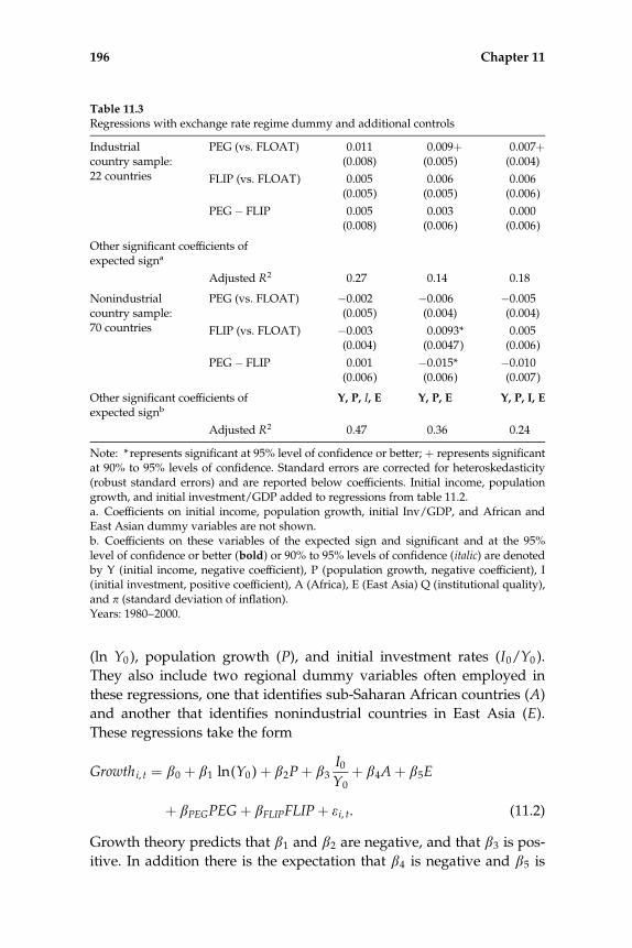
(ln Y0 ), population growth (P), and initial investment rates (I0/Y0 ).
They also include two regional dummy variables often employed in
these regressions, one that identifies sub-Saharan African countries (A)
and another that identifies nonindustrial countries in East Asia (E).
These regressions take the form
Growthi, t ¼ b0 þ b1 ln(Y0 )þ b2Pþ b3I0Y0
þ b4Aþ b5E
þ bPEGPEGþ bFLIPFLIPþ e i, t. (11.2)
Growth theory predicts that b1 and b2 are negative, and that b3 is pos-
itive. In addition there is the expectation that b4 is negative and b5 is
Table 11.3
Regressions with exchange rate regime dummy and additional controls
PEG (vs. FLOAT) 0.011 0.009þ 0.007þ(0.008) (0.005) (0.004)
FLIP (vs. FLOAT) 0.005 0.006 0.006(0.005) (0.005) (0.006)
Industrialcountry sample:22 countries
PEG� FLIP 0.005 0.003 0.000(0.008) (0.006) (0.006)
Other significant coefficients ofexpected signa
Adjusted R2 0.27 0.14 0.18
PEG (vs. FLOAT) �0.002 �0.006 �0.005(0.005) (0.004) (0.004)
FLIP (vs. FLOAT) �0.003 0.0093* 0.005(0.004) (0.0047) (0.006)
Nonindustrialcountry sample:70 countries
PEG� FLIP 0.001 �0.015* �0.010(0.006) (0.006) (0.007)
Other significant coefficients ofexpected signb
Y, P, I, E Y, P, E Y, P, I, E
Adjusted R2 0.47 0.36 0.24
Note: * represents significant at 95% level of confidence or better; þ represents significantat 90% to 95% levels of confidence. Standard errors are corrected for heteroskedasticity(robust standard errors) and are reported below coefficients. Initial income, populationgrowth, and initial investment/GDP added to regressions from table 11.2.a. Coefficients on initial income, population growth, initial Inv/GDP, and African andEast Asian dummy variables are not shown.b. Coefficients on these variables of the expected sign and significant and at the 95%level of confidence or better (bold) or 90% to 95% levels of confidence (italic) are denotedby Y (initial income, negative coefficient), P (population growth, negative coefficient), I(initial investment, positive coefficient), A (Africa), E (East Asia) Q (institutional quality),and p (standard deviation of inflation).Years: 1980–2000.
196 Chapter 11
positive. The literature reviewed in the previous section, as well as the
results presented in table 11.2, suggest that bPEG is negative (i.e.,
growth is slower under pegs than under floats). The effect of flips ver-
sus floats is less clear, but given the results in table 11.2, the question is
whether the positive value of bFLIP, which shows the effects of flips
compared to floats, is preserved with the inclusion of other variables.
Likewise there may be an expectation, given the results in table 11.2,
that the difference in the two coefficients bPEG � bFLIP is negative. A sig-
nificantly negative result would show that countries that peg grow
more slowly than countries that flip their exchange rate regime, condi-
tional on the other variables included in the regression.
The results presented in table 11.3 show that the inclusion of these
additional variables in the regression eliminates the significance of the
exchange rate regime dummy variables (at the 95 percent level of con-
fidence) for nonindustrial countries in the twenty-year panel and the
five-year panel. There is still a positive and significant effect of flipping
exchange rate regimes in the ten-year panel, both as compared to float-
ing and as compared to pegging. These significant coefficients are
smaller than those reported in table 11.2. The coefficients on initial in-
come, population growth, and the East Asian dummy variable are all
of the expected sign and significant at better than the 95 percent level
of confidence for the nonindustrial country sample. The coefficient on
the initial investment share is also significant and of the expected sign
in the five-year panel, and significant at the 90 percent level in the
twenty-year panel. Thus the results reported in this table indicate a
more limited role for the exchange rate regime for nonindustrial coun-
tries, but they still show a benefit of changing regimes (in the form of
flipping) as compared to pegging or floating, in the ten-year panel.
Before taking these results of the effects of exchange rate regimes on
growth as conclusive, however, we may be concerned with the role of
factors other than those typically incorporated in standard growth
regressions. This concern comes from the discussion in the previous
section, as well as the discussion in chapters 5, 9, and 11. The discus-
sion in chapter 5 shows that exchange rate regimes are typically linked
to institutional quality, and there is a literature that links institutional
quality to growth. The discussion in chapters 8 and 10 links the ex-
change rate regime to short-run macroeconomic performance, and the
short-run performance of the economy may spill over and affect its
long-run growth. We therefore run a set of regressions augmented
with two other variables, an indicator of institutional quality, Q, and
Economic Growth 197

the standard deviation of inflation, sd(p), to attempt to ensure that the
exchange rate regime is not serving as a proxy for institutional quality
or macroeconomic stability. Table 11.4 presents results for cross-
country growth regressions
Growthi, t ¼ b0 þ b1 ln(Y0 )þ b2Pþ b3I0Y0
þ b4Aþ b5Eþ b6Q
þ b7sd(p)þ bPEGPEGþ bFLIPFLIPþ e i, t (11.3)
where we expect that b6 is positive and b7 is negative.
Table 11.4
Regressions with exchange rate regime dummy and additional controls
Sample Coefficient 20 year 10 year 5 year
PEG (vs. FLOAT) 0.009 0.008 0.005(0.009) (0.005) (0.004)
FLIP (vs. FLOAT) 0.006 0.005 0.005(0.004) (0.005) (0.005)
Industrialcountry sample:22 countries
PEG� FLIP 0.003 0.003 0.000(0.008) (0.006) (0.006)
Other significant coefficients ofexpected signa
Y, p
Adjusted R2 0.34 0.16 0.22
PEG (vs. FLOAT) �0.002 �0.004 �0.004(0.005) (0.004) (0.004)
FLIP (vs. FLOAT) 0.001 0.008þ 0.005(0.004) (0.004) (0.006)
Nonindustrialcountry sample:70 countries
PEG� FLIP �0.003 �0.013* �0.009(0.005) (0.005) (0.006)
Other significant coefficients ofexpected signb
Y, P, p,
Q, A, E
Y, P, p,
I, A, E
Y, P, p,
Q, A, E
Adjusted R2 0.60 0.45 0.29
Note: * represents significant at 95% level of confidence or better; þ represent significantat 90% to 95% levels of confidence. Standard errors are corrected for heteroskedasticity(robust standard errors) reported below coefficients. Initial income, population growth,initial investment/GDP, institutional quality and standard deviation of inflation addedto regressions reported in table 11.2.a. Coefficients on initial income, population growth, initial Inv/GDP, and African andEast Asian dummy variables not shown (reported in the appendix to chapter).b. Coefficients on these variables of the expected sign and significant and at the 95%level of confidence (bold) or 90% level (italic) are denoted by Y (initial income, negativecoefficient), P (population growth, negative coefficient), I (initial investment, positivecoefficient), A (Africa), E (East Asia) Q (institutional quality), and p (standard deviationof inflation).Years: 1980–2000.
198 Chapter 11

The results presented in table 11.4 show that both institutional qual-
ity and the standard deviation of inflation are significant determinants
of growth in the twenty-year panel, while the former is significant in
the five-year panel and the latter is significant in the ten-year panel
(and significant at better than the 90 percent level of confidence in the
five-year panel). More to the point, the estimated effect of the exchange
rate regime on growth for the nonindustrial sample that was reported
in table 11.3 is very similar to that reported in table 11.4. The signifi-
cant difference between flips and floats in the ten-year sample drops
from better than 95 percent significance to significant at between the
90 percent and 95 percent levels. In the industrial country, sample the
positive and (somewhat) significant effects of pegs versus floats in the
ten- and five-year panels does not survive the inclusion of these two
additional regressors.
The overall results from the regressions presented in this section
suggest that there are important differences in the effect of exchange
rate regimes on growth between industrial and nonindustrial coun-
tries. There is some evidence that flipping—as opposed to staying in
one regime—is associated with faster growth in nonindustrial coun-
tries, even when controlling for other factors that may be associated
with the exchange rate regime. But this is a somewhat limited result,
and only found in ten-year panel regressions. There is little evidence
that the exchange rate regime is a significant determinant of growth
among industrial countries, even when one does not control for other
variables.
11.3 Conclusion
In standard models, long-run economic growth depends on real vari-
ables like the savings rate, the rate of population growth, and initial in-
come. These models have been augmented along several dimensions.
One line of research has explored whether nominal factors have an
effect long-run growth. One branch of that research has looked at the
potential impact of the exchange rate regime on long-run growth. As
discussed in section 11.2, this literature has come up with mixed
results, although there is some evidence that greater exchange rate
flexibility is associated with faster economic growth in nonindustrial
countries.
Our own results, presented in section 11.3, support the view that
there is little impact of the exchange rate regime on long-run growth.
Economic Growth 199

The literature has some well-known results that challenge the theoreti-
cal inconsequence of exchange rate regimes for long run growth. Levy-
Yeyati and Sturzenegger (2003) have argued that floats grow faster for
nonindustrial countries, and Husain, Mody, and Rogoff (2005) have
argued that industrial countries that float grow faster than industrial
countries that peg. We find support for neither hypothesis. In regres-
sions without proper controls we see pegs growing slower for nonin-
dustrial countries, but the result disappears with proper controls. The
only result that stands after proper controls are included is a weak re-
sult that countries that flip may grow faster than either long-term pegs
or long-term floats in nonindustrial countries (but only at the ten-year
horizon, not the five or twenty). This result, that neither pegging nor
floating but changing regimes is weakly beneficial in nonindustrial
countries, may be seen as consistent with the results of Ghosh, Gulde,
and Wolf (2002) in their finding of a positive growth effect for interme-
diate regimes. As noted above, they also argue exchange rate regimes
are generally not important for growth.
Thus, we do not see any compelling evidence that the exchange rate
regime affects the long-run level of output. This lack of a finding is con-
sistent with the general theory of long-run monetary neutrality. This is
not to say, however, that the exchange rate regime has no effect on the
behavior of real national income at shorter time horizons. By restricting
monetary autonomy, pegging may lead to more real income volatility
at the business cycle frequency because the central bank cannot re-
spond to shocks. As mentioned in chapter 8, the work of di Giovanni
and Shambaugh (2008) shows that real GDP growth rates of countries
that peg are reduced when the base country raises interest rates. This
is an important real consequence of the exchange rate regime, but it is
one that is distinct from long-run economic growth.
Appendix
Countries in analysis (92):
Industrial (22): Australia, Austria, Belgium, Canada, Denmark, Fin-
land, France, Greece, Iceland, Ireland, Italy, Japan, Luxembourg, Neth-
erlands, New Zealand, Norway, Portugal, Spain, Sweden, Switzerland,
United Kingdom, United States
Nonindustrial (70): Algeria, Argentina, Bahamas, Bahrain, Bolivia, Bo-
tswana, Brazil, Burkina Faso, Cameroon, Chile, Colombia, Costa Rica,
200 Chapter 11

Cote d’Ivoire, Cyprus, Dominican Republic, Ecuador, Egypt, El Salva-
dor, Ethiopia, Gabon, The Gambia, Ghana, Guatemala, Haiti, Hondu-
ras, Hong Kong, Hungary, India, Indonesia, Iran, Israel, Jamaica,
Jordan, Kenya, Korea, Madagascar, Malawi, Malaysia, Malta, Mexico,
Morocco, Nicaragua, Niger, Nigeria, Pakistan, Panama, Papua New
Guinea, Paraguay, Peru, Philippines, Poland, Qatar, Saudi Arabia, Sen-
egal, Sierra Leone, Singapore, South Africa, Sri Lanka, Sudan, Suri-
name, Syria, Tanzania, Thailand, Togo, Trinidad and Tobago, Turkey,
Uganda, Uruguay, Venezuela, Zimbabwe
Countries with twenty-year peg (18): Austria, Luxembourg, Nether-
lands, Bahamas, Bahrain, Burkina Faso, Cameroon, Cote d’Ivoire,
Egypt, Gabon, Hong Kong, Niger, Panama, Qatar, Saudi Arabia, Sene-
gal, Syria, Togo
Countries with twenty-year float (41): Australia, Canada, Finland,
Greece, Iceland, Japan, New Zealand, Norway, Portugal, Spain, Swe-
den, Switzerland, United Kingdom, United States, Algeria, Bolivia,
Brazil, Chile, Colombia, Costa Rica, Ecuador, Ghana, Hungary, India,
Israel, Kenya, Madagascar, Malawi, Malaysia, Malta, Morocco, Paki-
stan, Peru, Poland, Sierra Leone, South Africa, Sri Lanka, Tanzania,
Turkey, Uruguay, Zimbabwe
Economic Growth 201


V Conclusion

12 Exchange Rate Regimes in an InterdependentWorld
Perhaps no single price attracts as much attention as the exchange rate,
the price of one currency in terms of another. Certainly no other price
has an entire branch of economics dedicated to its study. In some
ways the exchange rate is simply an asset price like any other,
responding to fundamentals and expectations. At the same time it
serves as the translator of the value of goods, services, and assets in
one country compared to another. Consequently no other price has as
much government intervention as the exchange rate and the decision
of how to treat it—whether to fix its price or let it float and be deter-
mined by the market—is considered a crucial economic policy decision
for many countries.
In this book we have characterized this decision—the choice of the
exchange rate regime—and its impacts over the last thirty-five years.
The modern era, as we have dubbed it, differs crucially from previous
eras in that countries have a legitimate choice as to whether to peg or
float. Countries making different choices exist side by side at the same
time, and individual countries have changed policies frequently within
the era. A floating exchange rate, in the modern era, is not simply a
failure to peg and, thereby, to not participate in the international sys-
tem as in previous eras. Rather, floating is now a viable policy option
pursued by many countries, in some cases for long spells and in others
for brief episodes between pegging. Pegging is likewise a country’s
choice that is typically not linked to the decision of whether to join an
overarching system. We have documented the dynamics of this choice
as some countries have stayed in a particular exchange rate regime for
extended periods and many others have flipped back and forth across
regimes.
We have also shown the choices countries make with respect to the
exchange rate regime matter. First and foremost the exchange rate

regime has a substantial direct effect on the behavior of the exchange
rate itself, with floats exhibiting considerably more volatility than pegs.
Despite the fact that countries can only peg to one other currency,
even multilateral volatility, the average against other exchange rates,
shows significant differences across regimes. Unlike bilateral volatility
where floats and pegs are truly distinct, however, many floats have
low multilateral volatility. Also some pegged countries that peg to a
base that is moving against the rest of the world have some multi-
lateral volatility. But still, on average, pegs and floats are different on
both measures. Given these exchange rate effects, it is plausible the ex-
change rate regime will affect other economic outcomes, and we find
that it does.
As predicted by economic theory, monetary autonomy is severely
limited by pegging such that countries that peg and have an open fi-
nancial market are limited in their ability to set interest rates with
regards to local economic circumstances; instead, they must follow the
interest rate policy of the country to which they are pegged. At the
same time a pegged country does trade more with its base country
since nominal exchange rate volatility has been eliminated between
the two countries, and more importantly, there is more long-run cer-
tainty of the future exchange rate.
The constraint that pegging places on monetary autonomy means
that a fixed exchange rate disciplines the central bank and prevents ex-
tensive monetary easing. This leads to significantly lower inflation rate
in pegged countries. At shorter horizons, this effect operates even over
and above the direct effect that pegs have on limiting increases in the
money supply since pegs can establish low inflation credibility by pro-
viding a visible nominal anchor. In the long run, however, monetary
policy must match reputation, and the only impact of the exchange
rate regime is to discipline developing countries’ monetary policy
(advanced countries seem to be able to limit money growth with or
without a fixed exchange rate in the long run).
Finally, as important as exchange rate regimes can be, we would not
expect them to determine the long-run productive capacity of an
economy, even though they can affect real variables at shorter time
horizons. Long-run levels of national income are determined by
endowments, labor, capital, technology, and institutions. Over this ho-
rizon, it does not appear that fixing the currency, allowing it to float, or
flipping back and forth across these choices has an independent effect
on a nation’s standard of living.
206 Chapter 12

This book represents both new work and a synthesis of the recent
wave of research that show the exchange rate regime to be quite im-
portant to many economic outcomes in this modern era. As the mod-
ern era progresses and the choices and experiences of many countries
change and evolve, we are sure to learn more about exchange rate re-
gime choice and outcomes. We hope this book informs economists,
practitioners, and students about some of the important lessons
learned about this fundamental policy choice thus far in the modern
era.
Exchange Rate Regimes in an Interdependent World 207

Notes
Chapter 1
1. There were a variety of exchange rate regime choices during the two-decade interwarperiod, but this was a time of great economic instability. For an authoritative account ofthis period, see Eichengreen (1992).
2. See Bordo, Edelstein, and Rockoff (2002).
3. See Meissner (2005) for a discussion of the development of the gold standard.
4. International economists often refer to the period studied in this book as the ‘‘Post–Bretton Woods’’ era. But, since this period has, by now, lasted longer than the precedingBretton Woods era, it deserves its own name. We have chosen ‘‘modern era’’ because ithas a parallel in art history. The ‘‘modern period’’ of art is marked by a great heterogene-ity in styles and approaches existing side by side in the same time period.
5. Original contributions to the monetary approach to exchange rates include Frenkel(1976) and Bilson (1978). Boughton (1988) discusses the empirical failure of this model,although DeJong and Husted (1993) suggest this might be due to the low power of thetests used.
6. See Rogoff (2002) for a review of the influence of the Dornbusch overshooting model.
7. Theoretical research by Krugman (1979), Flood and Garber (1984), and Obstfeld (1994)offered frameworks for understanding these events. Empirical research on the anteced-ents to these crises (Berg and Pattillo 1999) and their effects, added importantly to ourunderstanding of some of the implications of the choice of a fixed exchange rate regime.
8. See Obstfeld and Rogoff (1995).
9. See Calvo and Reinhart (2002).
Chapter 2
1. For example, see Corden (2004) for a discussion of some of the current issues in ex-change rate regime debates.
2. Dollarization is simply dispensing with using a national currency and using the cur-rency of another country. A currency union involves creating a new common currency

across member countries and having supranational institutions (such as a central bank)to manage the currency.
3. See Krugman and Obstfeld (2008) for an explanation of the policy trilemma in the con-text of a simple macroeconomic model of an open economy. For a more advanced treat-ment, see Obstfeld and Rogoff (1996).
4. It is theoretically possible to break the policy trilemma if fiscal policy could be directedtoward exchange rate management while monetary policy was used separately to set in-terest rates. This is not a realistic situation, however, since fiscal policy is not nimbleenough to respond in a timely way such that it serves to peg the exchange rate. Alterna-tively, sterilized intervention, whereby the monetary authority alters the outstandingstock of assets denominated in domestic currency while maintaining separate controlover the money supply and interest rates, also breaks the policy trilemma. In this case,however, there is little empirical evidence that sterilized intervention has consistent andlong-lived effects on exchange rates except possibly as signaling future monetary policy.Since these signals need to be backed up by actual policy, sterilized intervention provideslittle promise of breaking the trilemma.
5. Even in a broad system where many countries peg together, most fixed exchange ratesystems have been asymmetric in that a ‘‘center’’ country has a free hand in setting policywhile all other participating countries direct their policies to the maintenance of the peg.In this case, the center country has both a fixed exchange rate (through the actions ofother countries) and a free hand to set its own monetary policy.
6. See Frankel (2003).
7. The argument about the way in which the relative merits of exchange rate regimesdepends on the source of shocks to an economy is an open-economy version of the wellknown analysis of Poole (1970).
8. The formal abandonment of the system of fixed but adjustable parities was made byan Interim Committee of the IMF at a meeting in Kingston, Jamaica in January 1976.
9. The Nobel Memorial Prize in Economics was awarded in 2004 to Finn Kydland andEdward Prescott for their contribution on policy credibility. See Kydland and Prescott(1977), as well as Calvo (1978) and Barro and Gordon (1983) for some early and influen-tial contributions.
10. For a review of these experiences, see Vegh (1992).
11. Klein and Marion (1997) show that a loss of competitiveness due to inflation in ex-cess of that of the base country is an important predictor of the end of a fixed exchangerate.
12. For example, Klein, Schuh, and Triest (2003) show that real exchange rates are an im-portant determinant of job destruction in US manufacturing industries.
13. See Frankel (1999).
14. OCA theory was originally concerned with the adoption of a single currency, but itsideas translate to issues of a fixed exchange rate as well.
15. It is important to recall, however, that the United States has not always had a singlecurrency. Up until the Civil War there were a variety of monies circulating. For a discus-sion of this see Sheridan (1996) and Shambaugh (2006).
210 Notes
16. For example, Bayoumi and Eichengreen (1998) compared the correlation of economicdisturbances across the countries of Europe to that across regions in the United States,and Blanchard and Katz (1992) considered labor mobility and fiscal transfers acrossstates in the United States, which serves as a benchmark for these features in Europe.Bean (1992) also offered a prospective view of monetary union in Europe.
17. A dominant international exchange rate system, such as the gold standard, can influ-ence national decisions about the choice of an exchange rate regime. See Broz (1997) andFrieden (1993).
18. We provide evidence in chapter 10 that fixed exchange rates between two countriespromotes trade between them.
19. Exporting and importing firms also serve the domestic market, so their desire for ex-change rate certainty versus policy flexibility when dealing with business cycles is notstraightforward.
20. Another issue that potentially limits the interest group influence on exchange ratepolicy can be understood by contrasting it with the interest group effect on trade policy.Legislation for specific tariffs or quotas can be very firm-specific, and, with these concen-trated benefits, there may be extensive lobbying. The benefits of exchange rate policiesare more diffuse and give rise to free riding and, therefore, a smaller interest group effect.
21. In his Nobel Prize acceptance speech, Robert Mundell suggested that these changesin the international monetary system were a crucial cause of many of the major economicand political events of the 20th century, ranging from the Depression, to the rise of fas-cism and World War II, to the inflation of the 1970s, to the subsequent rise of conserva-tive political forces. See Mundell (2000)
22. See Eichengreen (1996) and Obstfeld and Taylor (2004) for clear descriptions of thisera.
23. A handful of countries broke their peg to gold and re-pegged, but by and large, oncecommitments were made, they were locked in and, by 1905, nearly all countries with in-dependent economies were on the gold standard. We date the gold standard from 1880.In some countries, notably the United Kingdom, it began earlier, and between 1870 and1880 a number of countries joined. See Meissner (2005) for a description of the rise of thegold standard system.
24. See Obstfeld, Shambaugh, and Taylor (2004) for a discussion of the interwar years inthe context of the trilemma.
25. See Eichengreen (1992) and Eichengreen and Sachs (1985).
Chapter 3
1. Frankel (2004).
2. These reports were initially titled Annual Report on Exchange Restrictions, whichreflected the lack of variety of exchange arrangements during the Bretton Woods period.The title changed to Annual Report on Exchange Arrangements and Exchange Restrictions
with its 1979 volume.
3. Fischer (2001), using the classification scheme in the last column of table 3.1, places thecategory ‘‘conventional peg arrangements’’ into an intermediate regime, but one could
Notes 211

easily imagine this category combined with ‘‘no separate legal currency’’ and ‘‘currencyboards’’ into an aggregate peg category distinct from an intermediate regime that repre-sents limited flexibility.
4. Frankel et al. (2001) discuss the length of time it can take to discern the true weights ina basket. Given that if the weights are not declared, and that they may be changing overtime, it is very difficult, as a practical matter, to use a de facto method classify such coun-tries on an annual basis.
5. The Reinhart–Rogoff classification will code countries as following a de facto SDR pegsif it is a true de facto SDR peg, but this is a rare occurrence. More commonly, they codedeclared SDR pegs as nonpegs or as direct pegs to a particular base since few declaredSDR pegs are in fact SDR pegs.
6. Other classifications include Moreno (2001) and Dubas et al. (2005), among others, butthese three have been used most frequently in the literature and the choices they makespan many of the options allowing for a rich discussion of the issues involved. Ghosh etal. (1997) made an early contribution in adjusting de jure codes for clear errors and Ghoshet al. (2002) also make a de facto classification for the purpose of looking for a ‘‘consensus’’where de facto and de jure agree.
7. The least flexible arrangements are assigned the value 1 in the coarse grid, and themost flexible are assigned the value 5. The fifteen fine grid categories (and their assign-ments to the coarser grid) are: ‘‘no separate legal tender,’’ ‘‘preannounced peg or currencyboard arrangement,’’ ‘‘preannounced horizontal band that is narrower than or equal toe2 percent,’’ and ‘‘de facto peg’’ (coarse grid 1); ‘‘preannounced crawling peg,’’ ‘‘prean-nounced crawling band that is narrower than or equal toe2 percent,’’ ‘‘de facto crawlingpeg,’’ ‘‘de facto crawling band that is narrower than or equal toe2 percent,’’ and ‘‘prean-nounced crawling band that is wider thane2 percent (coarse grid 2); ‘‘de facto crawlingband that is narrower than or equal toe5 percent’’ ‘‘noncrawling band that is that is nar-rower than or equal toe2 percent,’’ and ‘‘managed floating’’ (coarse grid 3); ‘‘freely float-ing’’ (coarse grid 4); ‘‘freely falling (includes hyperfloat)’’ (coarse grid 5).
8. To determine the base country, this system tests the exchange rate against the dollar,all major currencies, and major regional currencies to find any potential fixed exchangerate relationship. When a country pegs or occasionally pegs, determining the relevantbase currency is straightforward. It becomes more difficult to assign a relevant base fornonpegged observations of countries that generally float, do not peg for a substantialamount of time, or switch base currencies. In these cases, judgment was used, and thebase is the currency with historical importance for the local country, the nearby dominanteconomy to which other currencies were pegged, or, if no other currencies seem a goodcandidate for the base, the US dollar as a default.
9. Again, most basket pegs either stay stable to one particular currency (in which casethey are coded as a peg) or appear to float either by changing weights frequently or sim-ply ignoring the basket index.
10. The use ofe1 percent bands rather thane2 percent bands, and the decision to in-clude single peg breaks, has little effect on the results in the paper. Only 5 percent ofobservations coded as pegs are realignments. 38 percent never have the exchange ratechange, 45 percent have changes but stay within 1 percent bands and the remaining 12percent move outside 1 percent bands but stay within 2 percent bands.
11. See note 7.
212 Notes

12. See also Klein and Shambaugh (2008), Shambaugh (2004) or Frankel (2003) for com-parisons of different de facto classification schemes. The statistics shown do not includecountries that have no legal tender or are part of a currency union with the base as thesesomewhat trivially generate agreement amongst all three classifications.
13. It should be noted that these statistics include Reinhart–Rogoff managed floats (fineclassification 12) as floats, not intermediate. If they are considered intermediate, 52 per-cent of Reinhart–Rogoff spells are coded as intermediate. This also drives down theirrate of agreement with other classifications since most others code the bulk of theseobservations as floats. If the managed floats are considered intermediate, the rate ofagreement with Reinhart–Rogoff drops to 62 percent for the Shambaugh classification,52 percent for the LYS classification, and 53 percent for the de jure classification.
14. See for example Ghosh, Gulde, and Wolf (2002).
15. It is worth noting that even different de jure codings, all of which rely on the sameIMF yearbooks, disagree because researchers differ in how they aggregate declaredregimes. For example, a ‘‘cooperative system,’’ which is how the EMS was listed, couldbe considered a peg or an intermediate regime. Likewise managed floats can be calledintermediates or floats. Thus, using de jure classifications does not change the fact that aresearcher must decide what behavior is considered a peg and what is not.
Chapter 4
1. The significance of exchange rate regimes for economic performance also depends ona significant de facto difference of exchange rate behavior across exchange rate regimes.The influence of the exchange rate regime would be limited if pegs did not really bindexchange rates because they were frequently broken, or if governments actually limitedexchange rate movements during times when countries were purportedly floating. Weturn to this topic in chapter 6.
2. Obstfeld and Rogoff (1995).
3. See Mussa (1989) and Flood and Rose (1995).
4. Frankel and Wei (1994) is an example of this literature, which focused on the effect ofexchange rate volatility, rather than exchange rate regimes, on bilateral trade. We returnto the issue of exchange rate regimes and trade in chapter 10.
5. There is reasonable evidence that nearly all single year pegs are in fact legitimate pegsand do not simply represent a random lack of volatility of shocks across two countries.There are 39 country–year observations that are single year pegs that are not alsodeclared pegs and are not classified as pegs by Levy-Yeyati and Sturzenegger or Reinhartand Rogoff. Within this set, the exchange rate of 12 single year pegs remained within ae1 percent band, a situation that is highly unlikely to have arisen accidentally. Thus wefocus on the 27 ‘‘questionable peg’’ observations that are within 2 percent bands and areneither declared nor identified as a peg by Reinhart and Rogoff nor by Levy-Yeyati andSturzenegger. This set of observations represents 20 countries and 16 different years,and, therefore, is not evidence of a lack of world volatility in a particular year or country.It also includes many country–year observations that are widely considered to be de factopegs, such as Malaysia and Indonesia in 1996, as well as countries whose currency wasclearly shadowing that of another country, such as Portugal in 1975, which was linkedto the DM unofficially in the snake. Other countries, such as India, Pakistan, Tunisia, andJamaica, all of which have two ‘‘questionable’’ single year pegs, have many other
Notes 213
unquestionable pegs in the sample, making it unlikely that the ‘‘questionable’’ peg is justan accident of coding. Thus, while the official Shambaugh classification does not includesingle year pegs, if it is important to include them for the question studied (as we feel it isin this case), it is probably accurate to consider them pegs.
6. Below we compare the results in table 4.1 to those obtained through the use of theother exchange rate regime classification schemes discussed in chapter 3.
7. We limit the sample to countries with populations of at least 400,000, in part to matchthe data set in Obstfeld and Rogoff (1995). The United States is not included in the sam-ple of 125 countries, nor do we include spells that represent currency unions.
8. There are 3,924 observations, rather than 125� 32 ¼ 4000, because 76 observationsrepresent currency unions.
9. See Klein and Marion (1997) and Obstfeld and Rogoff (1995).
10. In a second panel in their table 2, Obstfeld and Rogoff list 17 small countries that hadpegged to the US dollar for at least five years. They write ‘‘The striking conclusion fromtable 2 is that aside from some small tourism economies, oil sheikdoms, and highly de-pendent principalities, literally only a handful of countries in the world today have main-tained tightly fixed exchange rates against any currency for five years or more’’ (p. 87,italics in original).
11. The panel is roughly balanced with between 122 and 125 countries in the sample. Theslight variation comes from the fact that currency unions are eliminated from samplewith the exception of spells that began as pegs and converted to currency unions (e.g.,some EMU observations).
12. Pegs lasting at least 5 years in 2000 includes some oil countries and the CFA coun-tries, but also many EU nations as well as Argentina, China, and El Salvador. The fulllist is: Argentina, Austria, Bahrain, Belgium, Benin, Burkina Faso, Cameroon, Central Af-rican Republic, Chad, China, Comoros, Republic of Congo, Cote D’Ivoire, Denmark, Dji-bouti, El Salvador, Equatorial Guinea, Gabon, Hong Kong, Jordan, Lebanon, Lesotho,Luxembourg, Mali, Namibia, Nepal, Netherlands, Niger, Oman, Qatar, Saudi Arabia,Senegal, Swaziland, Syria, Togo, and the United Arab Republic.
13. The presence of ‘‘inconclusive’’ observations, and the lack of complete coverage, pre-vents the inclusion of exchange rate spells based on the Levi-Yeyati and Sturzenegger ex-change rate classification scheme.
14. The Reinhart–Rogoff and IMF classification schemes could be used to generate aspell-based analysis in which there were more than two types of spells, but we continueto focus on a bivariate scheme for purposes of comparison and also because it offers acleaner and less ambiguous classification system than one that includes a category of‘‘limited flexibility,’’ or some other type (or types) of intermediate regimes.
15. See Kiefer (1988) for a good introduction to duration analysis and hazard functions.
16. Research by Masson (2001), Masson and Ruge-Murcia (2005) and Eichengreen andRazo-Garcia (2006) is related to this analysis, although these papers focus on whetherthe international monetary system is moving toward an ‘‘empty middle’’ consisting ofmainly currency unions, on the one hand, and free floats, on the other, or, alternatively,whether transitions are slow and countries shift back to the middle, not exclusivelyaway from it. These papers look at switching propensities across hard pegs, intermediateregimes (including pegs) and floats. Their results are related to our observations that nei-
214 Notes
ther pegging nor floating is an absorbing state, and flipping back and forth is common.The focus in these papers on extreme polar cases, and the inclusion in the broad middleband of what we define as both pegs and nonpegs, however, distinguishes this workfrom those papers.
17. Hazard functions may or may not be monotonic. Some hazard functions have deriv-atives that change sign for different values of t.
18. The covariates are not intended to be exhaustive, but rather illustrative. Klein andMarion (1997) provide an example of a detailed analysis of the end of a peg. We keepthe list of covariates limited for comparability across the peg and float spells.
19. The estimated l is less than one and significant even if no covariates are included. Forpeg spells the estimate of l is 0.798 with a standard error of 0.032, and for float spells theestimate of l is 0.845 with a standard error of 0.034.
20. The United States is the base country for 51percent of the pegs in this sample. Theother base countries include France (the base for 27 percent of the pegs), South Africa (6percent), the United Kingdom (2 percent), Belgium (1.5 percent), India (1 percent), Por-tugal (less than 1 percent), Malaysia (less than 1 percent), and Australia (less than 1percent).
21. Thirty-three pegs that broke re-formed within a six- to ten-year gap, leaving 91 (27percent) that do not re-form for at least ten years (or did not re-form by the end of thesample period). Eighteen of the breaks that did not re-form involve switches in the basecountry and, in these cases, countries may not have floated, but the original peg is notreconstituted if there is a peg to another base (most of these involved switches from theBritish pound sterling as the base to the US dollar during the 1970s).
22. Because they so distort the average, we calculate the average without including threeextreme outliers: Nicaragua in 1988, Surname in 1994, and Zimbabwe in 2003. In addi-tion, when these breaks re-form (Nicaragua after 4 years and Suriname after 2 years)they are again excluded from the average.
23. The Shambaugh and Reinhart–Rogoff classifications in fact refer to these as pegs,allowing for a break in the rate as long as the overarching regime has not changed.
24. This is not to argue that no countries manage their exchange rates if they are not liter-ally pegged, nor that no countries mis-declare their regimes. Rather, our point is thatsome countries actually do float and their exchange rates are notably more volatile thanthose that peg.
25. The implications of these distinct effects between bilateral and multilateral outcomesrelate to differences in trade and macroeconomic outcomes since bilateral volatility affectsbilateral trade and macroeconomic stability while economic growth, for example, may re-quire a broader effect across many sectors that is more closely associated with multilat-eral stability.
Chapter 5
1. Currency union countries will not be included in the empirical analysis in this chapter.
2. The question of the determinants of exchange rate regime choice is different from thatof the factors that contribute to the end of a pegged exchange rate spell. The distinctionbetween these two questions is discussed further in the next section.
Notes 215

3. In this context, the difference between a currency union and a fixed exchange rate isthe greater perceived permanence of the former relative to the latter. As shown in chapter9, both fixed exchange rates and currency unions promote bilateral trade. Also, as shownin chapter 8, the macroeconomic constraints imposed by pegging a currency for a coun-try whose government allows capital mobility hold for fixed exchange rates as well.Therefore Mundell’s OCA analysis is relevant for fixed exchange rates, and not just cur-rency unions.
4. Recall that if there are n countries in a currency union, n� 1 countries must follow themonetary policy of the central country unless the currency union is truly symmetric, inwhich case no country has a free hand in setting its own monetary policy.
5. As shown in chapter 9, a fixed exchange rate positively affects trade between twocountries, so there is some potential for endogeneity by which the dependent variable, re-gime choice, affects the regressor, the level of trade.
6. This would not hold, of course, for countries that have high levels of income per capitabecause of an abundance of a natural resource like oil. One could easily control for this ina regression by including a variable to capture a country’s dependence on oil exports, orby including a dummy variable that identifies major oil exporters.
7. This is a distinct reason from the issue of the natural level of trade of an economy thatis dominated by the production of a single good, although both of these affect the prefer-ence for a peg relative to a float in the same direction.
8. Distance could change with the change in the base country, but this is a rare occur-rence. More important, Feyrer (2008) has shown that there has been a shift in interna-tional trade from shipping by sea to shipping by air. This has implications for the costsof transport and the effective distance between trading partners.
9. Important theoretical contributions include Krugman (1979), Flood and Garber (1984),and Obstfeld (1994). Various empirical approaches to this topic are evaluated by Bergand Pattillo (2002) in the context of the Asian financial crisis of the late 1990s.
10. Although there is some research on exchange rate regime choice in the interwar pe-riod. See, for example, Eichengreen (1992). There has also been interesting work recentlyon the spread of the gold standard. See Meissner (2005) and citations therein.
11. Other variables studied by Rizzo that are not associated with OCA theory, such asterms of trade, government revenue, the current account balance, the level of externaldebt, and the government budget deficit, are less consistently associated with exchangerate regime choice.
12. Alesina and Warner (2006) also consider sources of differences in the de facto and de
jure exchange rate regimes. They find that the de facto pegs of countries with poor institu-tions tend to break. Countries with good institutions are more likely to have de facto pegsthan de jure pegs, that is, they actually peg more often than they announce that they peg,which is consistent with the Calvo and Reinhart (2002) ‘‘fear of floating’’ result.
13. In contrast, time-varying dummy variables that indicate the year just before an elec-tion and the year just after an election (when, respectively, a float is more likely and apeg is more likely, extending the political business cycle logic from the cross section tothe time series) are not statistically significant.
14. A similar result is presented by Meon and Rizzo (2002).
216 Notes
15. Carmignani, Colombo, and Tirelli (2008) report a significant effect of political frag-mentation on increasing the likelihood of a de facto floating exchange rate in their sampleof 96 industrial and developing countries.
16. A linear probability model might be inappropriate if the impact on the choice is non-linear and a logit or probit model might be preferable if the functional form imposed bythose techniques better fit the data. A linear model can impose an unrealistic shape onthe predicted values (predicting results below zero or above one) but that is not a prob-lem in this case. Our predicted values rarely stray above one or below zero. Further,there is no evidence that the specific nonlinear model of a probit fits better and the linearmodel offers much more straightforward interpretation.
17. A discrete choice analysis would not allow a pure cross section of the full panel as thedependent variable would not be binary, but the percentage of time a country waspegged.
18. Geographical variables (distance, contiguous, colonial status, landlocked status)come from the CEPII database of geographical data. Macroeconomic data such as GDP,population, government share of the economy, and trade share, come from the WDI. Fi-nancial openness is from Edwards (2005) and democracy and corruption data are fromthe International Country Risk Guide published by the PRS group.
19. We use the Klein-Shambaugh de facto classification in which devaluations count as abreak in a peg. Results are very similar using the Shambaugh or Reinhart–Rogoff classifi-cations. One exception is that using the Reinhart-Rogoff classification leads to a resultwhere open financial markets are significantly associated with pegging (even more oftenthan the results presented here). This is because countries that peg the official rate buthave capital controls and have a diverging black market rate will not be considered pegsin the Reinhart–Rogoff classification.
20. It is important to note that studies that do not appropriately control for serial correla-tion will have incorrectly low standard errors and present a disproportionate number ofsignificant coefficients. In the regression in column 1 of table 5.1, 5 of 11 variables havecoefficients statistically different from zero at the 95 percent confidence level. Had thestandard errors been estimated in a standard manner, or only robust to heteroskedastic-ity, 8 of the 11 would have appeared significant.
21. Half the 35 countries eliminated have populations less than 800,000 in 2000, whileonly 5 percent of the remaining sample is as small. Of these 35 countries, 66 percentare pegged as opposed to 40 percent of the remaining countries, and average GDP percapita is less than $2000 (in 1995 US dollars) as opposed to over $6000 for the remainingcountries.
22. While most countries that peg do not, in fact, border their base, it is the converse thatdrives this result; a majority of countries that border their base country peg. Examples in-clude European countries like France and Austria, countries on the subcontinent that pegto India, and countries in southern Africa that peg to South Africa.
23. There is little difference in any of these results if we restricted ourselves to a later(post-1989) sample.
24. As noted, once a peg has commenced, some variables (e.g., real exchange rate appre-ciation) can tell us about the likelihood of the peg collapsing, but these are not necessarilycorrelated with floating in general as much as with a peg breaking. Further, these
Notes 217
variables are of no help in informing us as to when a peg will re-form; thus they are oflimited information regarding the flipping nature of pegs.
25. Our data set stops in 2002 (in part due to the political variables) but this is convenientbecause it means that we can tell if a peg that began in 2000, or even 2002, did in fact lastfor a full five years.
26. Here a point raised in Klein and Shambaugh (2008) is relevant. While a majority ofpegs break quickly—and hence a majority of peg spells are classified as short pegspells—long pegs are observed far more frequently in annual data (because each yearthat they last represents an observation) and hence the panel estimation in table 1 islargely based on longer pegs.
27. Seventy-five percent of the countries coded as flippers spent at least half of their timein short spells. The remaining 25 percent did spend a fair amount of time in both longpegs and long floats, but also flipped a number of times.
Chapter 6
1. Calvo and Reinhart focus on de jure, not de facto, pegs, and show that many countriesthat say they float do not really do so. But this paper has had a strong influence and itsmessage has sometimes been extrapolated more broadly to mean that floats do not reallyfloat at all.
2. Grilli and Kaminsky (1991) worried that the results could be driven by differences ineras rather than regimes since so much of the regime differences were Bretton Woodsversus non Bretton Woods. Mussa, though, uses Canada’s float during Bretton Woodsand Ireland’s switch of base country from United Kingdom to Germany as counterpointsand, in response to Grilli and Kaminsky’s argument, Liang uses exchange rate regimesfrom the modern era for his tests.
3. The bilateral exchange rate used to calculate volatility is the month end official ex-change rate, converted to be the bilateral exchange rate against the relevant base country,reported in line ae in the International Monetary Fund’s IFS database. This measure ofvolatility does not line up exactly with the rule for coding an exchange rate experience asa peg regime in the Shambaugh or Klein–Shambaugh classification schemes since the ex-change rate regime coding requires staying within a tight range over the course of a year.For example, a country with a steady crawling peg may exhibit low exchange rate volatil-ity from one month to another but it would not be classified as having a peg if it violatesthe condition of staying within a 2 percent band over the course of a year.
4. As in chapter 4, the sample used does not include very small countries or countriesthat maintain a currency union with their base country.
5. A similar analysis using the peg and float spells discussed in chapter 4 produces verysimilar results. See section 6.4 and Klein and Shambaugh (2008) for more results.
6. Including the ‘‘soft peg’’ marker shows that all the nonpegged observations in the sec-ond and third quintiles are soft pegs, meaning the gap between true pegs and true floatsis even larger.
7. The end of the chapter examines these results across different exchange rate regimeclassifications discussed in chapter 3.
218 Notes
8. A significant difference between this discussion and research that studies bilateral vol-atility overall is our focus on volatility against the base country. Lane and Devereux(2003) is a leading example of tests of bilateral volatility across many country pairs. Intheir work, the goal is to explain why countries may try to lower exchange rate volatility,rather than the impact of exchange rate regimes as we study here. Many of their variables(e.g., distance or debt burden) are time invariant across countries or close to being so. Assuch, our use of country fixed effects eliminates most comparisons between the works.They find that bilateral external debt is a significant explanatory variable in explainingvolatility for developing countries, and that general optimal currency variables (trade,correlation of shocks, country size) are more important for industrial countries.
9. Standard errors are clustered at the country level. This allows for an unstructuredautocovariance matrix that can correct for heteroskedasticity and autocorrelation. The de-pendent variable EVOL is persistent, but nowhere near unit root levels (autocorrelationcoefficients range near .3) suggesting this correction is sufficient to handle time seriesissues relating to the use of panel data. See Bertrand et al. (2004) for discussion.
10. That is, if one takes the standard deviation of a year in which the change in the ex-change rate for six of the months is 16 percent each month and the change in each of theother six months is �16 percent, the resulting standard deviation is roughly 0.16. On theother hand, if not all the observations are at the boundaries, the range could be larger.That is, .16 is also the standard deviation if the change in the exchange rate in 3 of themonths is 21 percent, in another 3 of the months is �21 percent, in a third set of 3 monthsis 7 percent, and in each of the remaining 3 months is �7 percent. Thus the volatility mea-sure does not directly translate into a specific range, but gives us a sense for the size ofthe range. The average annual range of a float in this sample ise14 percent (the medianise6 percent).
11. See Klein and Shambaugh (2008) for further robustness checks on these results. Theexclusion of country fixed effects makes little difference. Dropping the first year of a floatspell, so that a potential crisis year is not included in the overall subsequent float spell,has some effect (with the absolute value of the coefficient falling to 0.045), but the differ-ence between pegs and floats is still highly significant.
12. Results across classifications are shown in section 6.4. Of particular interest is the factthat consistent with Calvo and Reinhart (2002), de jure pegs have a statistically insignifi-cant effect on volatility.
13. As in the spells estimates, including such observations just makes the gap betweenpegs and floats bigger, but including them leaves a false impression of the typical experi-ence of floats.
14. The top 1 percentile of volatility observations are excluded, as in column 1 of table6.2. We do not include the first-year float variable. By controlling for these separately,when we look at lagged pegs, we would eliminate some of the largest volatility outcomesfor previous pegs and thus artificially increase the difference between lagged pegs andfloats.
15. The sample does not include countries that floated at time zero but begin to peg inthe next 1, 2, 3, 4, or 5 years. The result is a comparison of countries that had pegged attime zero (regardless of what they are doing now) with countries that floated at timezero and are also floating at time 1, 2, 3, 4, or 5, depending on the lag used in the bivari-ate regression. We want to examine whether pegs at time zero have lower volatility inthe future, not whether pegs at time zero have lower volatility in the future than floats at
Notes 219
time zero. Pegs that continue will have lower volatility, but many of the broken pegs willre-form.
16. Ghosh et al. (2002) also examined volatility over time and also found lower volatilityfor pegs, but they restricted their sample to regimes that stayed pegged or stayed float-ing, eliminating the important role of pegs breaking or re-pegging.
17. We note that the de jure result is not simply due to declared floats not floating but,more important, is due to the highly volatile observations, which are labeled as pegs inthe de jure coding.
18. Friedman (1953) argued that given underlying instability in an economy, ‘‘freezing ofexchange rates cures none of the underlying difficulties and only makes adjustment tothem more painful,’’ while floating allows ‘‘continuous sensitivity’’ to changes in real con-ditions and hence smoothes adjustment.
19. The results in section 6.4 also hint at this result. Both the JS and RR classificationsshow lower volatility for pegs than floats despite the fact that both count discrete devalu-ations (or adjustments in the adjustable pegs) as part of a pegged regime.
20. Asici, Ivanova, and Wyplosz (2005), in their study of the consequences of ending apeg, show that the likelihood of a disorderly exit from a peg spell increases as the dura-tion of that spell increases.
Chapter 7
1. Countries sometimes peg to a basket of currencies, a topic we examine later in thischapter. The weights assigned to currencies in the basket typically are not declared (al-though an alternative way to peg to a basket of currencies is to peg to some known com-posite, like the SDR).
2. Dubas, Lee, and Mark (2005) take an alternate tack by using the multilateral rates todetermine exchange rate regime status. They argue that a peg is ineffective, and not reallya peg at all, unless it truly stabilizes the multilateral rate.
3. This is not true for all countries. Some developing countries that peg to bases otherthan the US dollar still have considerable US dollar liabilities in part due to their debts tomultilateral organizations such as the World Bank or the IMF.
4. The real exchange rate data (line rec) is available for fewer countries, roughly 93. Inmost of our tables, there will be 120 countries in the nominal volatility regressions androughly 70 in the real volatility regressions.
5. As discussed in chapter 6, country fixed effects control for differences in the character-istics of countries that tend to peg rather than float, and lessen concerns of omitted vari-able bias. Not including the country fixed effects has a relatively small impact on theresults. In a few cases the coefficients are smaller, but never significantly so.
6. As in chapter 6, the standard errors are clustered at the country level.
7. We also report the results after dropping the top 1 percent of volatility outliers. In thiscase, it makes little difference.
8. We use the most data that are available, therefore the sample for real and nominal aredifferent. As it turns out, there is no difference if we limit the estimates for nominal vola-tility to a sample where real exchange rate data is available.
220 Notes

9. There is little difference in the results across industrial and developing countries. Theoverall volatility levels for rich countries are lower, and hence the coefficients on the pegvariable are lower, but the share of variation in volatility that pegging can explain is con-sistent across the two samples.
10. Controlling for inflation does cut the size of the peg coefficient, but it is still statisti-cally significant. Controlling for inflation may not be appropriate. If we think the channelthat allows pegs to generate lower volatility is by providing a nominal anchor and thushaving less inflation, it is possible that we should view the inflation impact on volatilityas being related to the peg decision. See chapter 11 for more on this topic.
11. Empirically it can be quite difficult to verify the weights used in a basket, and hencedifficult to distinguish a basket peg from a managed float, as discussed by Frankel et al.(2001).
12. We can also include controls for the share of trade with the base country, and thathas no impact on the results. Thus it is not simply that pegs have lower volatility becausethey have stabilized trade with the base country. There is in fact no difference in tradeshare with the base country across the five quintiles of real or nominal volatility for eitherpegs or floats.
Chapter 8
1. This section is derived from Shambaugh (2004). See the full paper for more details.
2. The argument here is similar to that of uncovered interest parity (UIP), but it is lessstrict and does not require that UIP hold for all countries. Rather, this argument simplysays if you take away the uncertainty and the exchange rate is pegged, then the resultsdescribed must hold. In contrast, UIP can (and does) tend to fail for countries where thereis large uncertainty in the exchange rate market and the currencies float.
3. There have been other recent studies that focused on subsets of countries. Abraham(1999) examines the relationship of Saudi Arabia’s interest rate to the US rate; Cheung,Tam, and Yiu (2008) examine China’s relationship with the United States; Kim and Lee(2008) look at a number of Asian countries; and Hakura (2005) examines shifts in auton-omy as some emerging market countries begin to float.
4. Since the data will be differenced, the first year of a peg cannot be used as that obser-vation will difference from a peg to a nonpeg observation. Thus the single-year pegsincluded in the Klein–Shambaugh data set will all be dropped, making the difference be-tween the two classifications fairly small.
5. While we might prefer a de facto measure of capital controls, a number of them eitherhave very limited availability or require the use of interest rate movements (exactly whatwe want to test) to determine financial openness.
6. Obstfeld, Shambaugh, and Taylor (2004) also examine results for the interwar yearsbetween World War I and World War II. Those results are consistent with the findingsdescribed in the text.
7. As in previous chapters, a country is assigned a base even when it does not peg. Thebase is the country to which a country would peg if it is pegged. The base is revealedsince most countries peg at some point. In the rare instances it is not, we rely on currencyhistory, a dominant regional economy, or the US dollar. See Shambaugh (2004) fordetails.
Notes 221
8. We use the changes in annual interest rates. Differencing the data removes any con-stant risk premium or expected depreciation from the data (as well as other details suchas differential tax treatments that might make the assets imperfect substitutes). In addi-tion, levels of nominal interest rates often behave very close to unit root series. Thiswould raise the possibility of spurious regressions, making differencing the data prefera-ble. Technically the interest rates are expressed as ln(1þ R). This both reduces the impactof outliers and matches the theoretical derivation of the equation. See Shambaugh (2004)for details of both issues.
9. The sample involves all three eras in the pooled era. The results are drawn from thesample of countries that have interest rates that show some changes over a two to threeyear horizon. The papers eliminate countries that set interest rates administratively andnever change them. See Obstfeld, Shambaugh, and Taylor (2005, tab. 2) and Shambaugh(2004, tab. 5) for details.
10. Both papers experiment with the additional interaction of (peg� open financial mar-kets). In theory, the trilemma would say only open financial market pegs show any re-sponse to the base. In fact, the results consistently show the effects of pegging andcapital controls are additive, not multiplicative. That is, either opening the financial mar-kets or pegging generates a loss of some autonomy and doing both generates a loss ofeven more.
11. Shambaugh (2004) shows that adding other variables interacted with the base inter-est rate, such as trade with the base country, controls for level of economic development,or external debt do not significantly move the coefficient on the peg variable. In relatedwork on a different topic, di Giovanni and Shambaugh (2008) also show that the coeffi-cient on the peg variable remains significant in estimates based on a different sample,with controls for local inflation or base country GDP growth.
12. See Shambaugh (2004, tab. 8). In this case the results show that as expected bytheory, the interaction term of (peg� open financial markets) is positive and significantand when it is included, peg and financial openness on their own are not significant.This would suggest open capital market pegs face the strongest monetary autonomyconstraint.
13. This technique, developed by Pesaran, Shin, and Smith (2001) allows for differentcritical values for series that are unit roots and non-unit roots. Thus, if a result is aboveor below both sets of critical values, we can ascertain if there is a relationship withouthaving to take a stand on the order of integration of the data. See Shambaugh (2004) fordetails on the technique and Obstfeld et al. (2005) for more detailed results.
14. There is a long literature on this topic, exemplified by the work of Giavazzi andPagano (1988).
Chapter 9
1. Nurkse (1944). Quoted in Kenen (1984).
2. Committee for the Study of Economic and Monetary Union, Report on Economic andMonetary Union in the European Community (Delors Report), 1989. Quote is from point26, p. 21.
3. The 1989 Delors Report called for a move to a single currency to support the singlemarket, and the phrase ‘‘One market, one money’’ served as the title of a 1992 report bythe European Commission (Emerson et al. 1992).
222 Notes

4. Those countries are: Austria, Belgium, Cyprus, Finland, France, Germany, Greece, Ire-land, Italy, Luxembourg, Malta, The Netherlands, Portugal, Slovakia, Slovenia, andSpain. Kosovo and Montenegro also use the euro as a de facto currency and special mon-etary agreements have been made with Monaco, the Vatican City, San Marino, and An-dorra where the euro is used as the currency in these small countries as well.
5. More recently Bergin and Lin (2008) have expanded this analysis to examine in whatway trade is altered by exchange rate regimes. They suggest that currency unions mayhave more of an effect on the extensive margin of trade (new firms exporting or newproducts traded) while fixed exchange rates may have more of an effect on the intensivemargin (trading more of the same goods by the same firms).
6. Theory also suggested, however, that the greater volatility of profits associated withgreater exchange rate volatility could increase profits, due to Jensen’s inequality. Thissuggests the possibility of an increase in trade with higher levels of exchange rate volatil-ity. For example, see Franke (1991).
7. The indicators of exchange rate risk vary across papers. Some of these include the ab-solute percentage change in the nominal bilateral exchange rate, the average absolute dif-ference between the forward rate and the realized spot rate, the variance of the exchangerate around a trend, a moving average of the standard deviation of the exchange rate,and exchange rate variances calculated from an ARCH or a GARCH model.
8. This short synopsis cannot cover the large literature on the relationship between ex-change rate volatility and trade. For a survey, see McKenzie (1999).
9. See Gagnon (1993) for more discussion.
10. Of course, exchange rate regimes refer to nominal exchange rates, not real exchangerates, and much of the work on volatility and trade focused on real exchange rate volatil-ity. But there is a very high correlation between real and nominal exchange rate volatilityin the modern era for the industrial countries that made up the samples in the majority ofthese studies.
11. Subsequent work on the role of currency unions on trade co-authored by Roseincludes Frankel and Rose (2002), Glick and Rose (2002), and Rose and van Wincoop(2001). Other work that revisits the effect on trade of membership in a currency unionincludes Barro and Tenreyro (2003), Edwards (2001), Nitsch (2002a, 2002b, 2004), Persson(2001), Pakko and Wall (2001), and Thom and Walsh (2002).
12. We discuss gravity models in detail in the next section.
13. For example, Frankel and Rose (2002) present an estimated coefficient on the cur-rency union dummy variable of 1.38 in their table 1, with an associated standard error of0.19. This suggests that membership in a currency union triples bilateral trade, ceteris par-ibus (since e1:38 � 1 ¼ 2.97).
14. Quah (2000), in his comment on the original Rose (2000) paper, notes that the absenceof a significant effect of exchange rate volatility on trade, combined with the strong, sig-nificant effect of currency unions, implies a large discontinuity in the effects on trade ofrestricting exchange rate volatility.
15. There is evidence that the pre–World War I gold standard had an important role inpromoting trade, and its demise contributed in an important way to the reduction inworld trade in the interwar period. See Eichengreen and Irwin (1995), Estevadeordal etal. (2003), Lopez-Cordova and Meissner (2003), and Rischl and Wolf (2003).
Notes 223
16. Rose (2000) distinguishes between currency unions and fixed exchange rates, writing‘‘Sharing a common currency is a much more durable and serious commitment than afixed rate’’ (pp. 10–11). Tenreyro (2007) writes, ‘‘the findings from currency unions donot generalize to other regimes with lower variability.’’
17. This section draws from Klein and Shambaugh (2006).
18. Anderson (1979) and Bergstrand (1985) provide early theoretical justifications for thegravity model.
19. We discuss the implications of the multilateral resistance terms for estimation of thegravity model below.
20. There is a more explicit theoretical backing for the fixed effects as well. Anderson andvan Wincoop (2003) discuss the importance of taking into account multilateral trade re-sistance terms, when estimating the gravity model and when interpreting its results. Oneway to take into account multilateral resistance is by including CFE. In a subsequentpaper (Anderson and van Wincoop 2004), they also mention that multilateral resistancemay change over time, and, for this reason separate country fixed effects should beincluded for each year in a panel setting (CYFE). In our data set, there are about 100observations for every country in every year (one for each trade partner). Country yearfixed effects will control for whether trade is differentially higher with a pegged tradepartner in years that a country pegs than with any other trade partner that year.
21. The results in this section draw on Klein and Shambaugh (2006).
22. The actual set of variables that constitute Xi, j, t used in the regressions include theproduct of the natural logarithm of income of countries i and j in period t, the product ofthe natural logarithm of income per capita of countries i and j in period t, a dummy vari-able indicating whether the two countries had a free trade agreement at time t, and an-other a dummy variable indicating whether one country was a colony of the othercountry at time t. The variables used in the regressions that do not vary over time, repre-sented by Zi, j, include the natural logarithm of the distance between countries i and j, theproduct of the natural logarithm of the land areas of countries i and j, dummy variablesrepresenting whether or not countries i and j share a common border or share a commonlanguage, and other dummy variables indicating whether one country had been a colonyof the other, whether either country is landlocked, whether either country is an island,whether both countries had a common colonizer, and whether one of the countries was,at one time, a dependency, territory, or colony of the other.
23. The partial derivative of trade with respect to either a fixed exchange rate or a cur-rency union could include both the direct effect and the separately estimated effect of areduction in exchange rate volatility. In practice, however, the estimated effect of ex-change rate volatility on trade is small and we only refer to the estimated direct effects.
24. The currency unions observations represent a small portion of world trade since theyoverwhelmingly represent trade between two developing countries.
25. These results are from Klein and Shambaugh (2006). The standard errors reported inthe regressions are clustered at the country pair level. This both allows for different vari-ance across the pairs and, more importantly, for an unstructured covariance within theclusters allowing for correlation across time. See Klein and Shambaugh (2006, n. 25) formore discussion.
26. Klein and Shambaugh (2006) provide results based only on trade among developingcountries, only among industrial countries, and only between industrial and developing
224 Notes
countries. They show that the significant role that currency unions play in promotingtrade is a result of bilateral trade among developing countries since there are very fewobservations from which to draw information about currency unions impact on indus-trial/developing dyads.
27. Glick and Rose use CPFE on a larger sample with more switches and find that whilethe effect is substantially lower than when estimated with CFE, there is still an economi-cally large effect on trade from a currency union. Klein and Shambaugh (2006) presentsome evidence on a sample that includes the Bretton Woods era in addition to the mod-ern era as well.
28. Klein and Shambaugh (2006) also present a range of other results that include consid-eration of effects within subsamples, the dynamics of pegs, and other estimation meth-ods. Results presented in this chapter are robust to these alternatives.
Chapter 10
1. Seminal theoretical works in this area include Kydland and Prescott (1977), Calvo(1978), Barro and Gordon (1983), and Rogoff (1985).
2. For example, see Alesina and Summers (1993) or Cukierman (1992).
3. In fact, there is more agreement that Friedman and Schwartz’s dictum holds at longhorizons than at shorter time horizons.
4. The exchange rate has been used as the centerpiece of disinflationary policies in manycountries, although these policies have met with mixed success. Vegh (1992) discussesthe role of the exchange rate as a nominal anchor in a number of efforts to stop highinflation.
5. Other theories, and previous empirical research, suggest some additional explanatoryvariables that we will include in the empirical analysis in section 10.3.
6. This would be consistent with the results presented in chapter 6 that show an absenceof the ‘‘fear of floating’’ since those results demonstrated a significant and economicallymeaningful difference in exchange rate volatility under pegged and floating exchangerates.
7. For more on this topic, see the survey by Calvo and Vegh (1999).
8. A third type of study considers the prevailing exchange rate regime on worldwide in-flation. See, for example, the analysis of the effects of the move from the Bretton Woodssystem to generalized floating on worldwide inflation by Crockett and Goldstein (1976)in the IMF Staff Papers. At the outset of the modern era, when inflation was endemicacross the world and the heterogeneity of exchange rate regimes in the post-BrettonWoods era was not foreseen, this issue was a source of special concern. The topic becameless pressing with the subsequent fall in inflation rates, first among industrial countries inthe early 1980s and, after this, among a very wide set of other countries. This general de-cline in inflation has been called ‘‘The Great Moderation.’’
9. An important consideration in this study, and the others cited here, is the potentialrole played by outliers that had very high rates of inflation. Ghosh, Gulde, Ostry, and
Wolf use p ¼ d ln(P)
1þ d ln(P)as a measure of inflation, which mitigates the effects of outliers.
Other studies drop observations representing extremely high rates of inflation.
Notes 225

10. The inclusion of openness is meant to capture the higher costs of monetary expan-sions in open economies, as discussed in Romer (1993). We return to this point below.
11. Lane (1997) also presents an alternative theory for why inflation and openness areinversely related.
12. The set of industrial countries includes the United States, the United Kingdom, Aus-tria, Belgium, Denmark, France, Germany, Italy, the Netherlands, Norway, Sweden,Switzerland, Canada, Japan, Finland, Greece, Iceland, Ireland, Portugal, Spain, Australia,and New Zealand.
13. The developing countries with high-inflation experience include Argentina, Bolivia,Brazil, Ghana, Israel, Mexico, Peru, Suriname, Turkey, Uganda, and Uruguay.
14. These regressions, and all the others reported in this chapter, adjust standard errorsfor heteroskedasticity and serial correlation by clustering at the country level.
15. Thus it seems that if there is a credibility effect in the developing sample, it is limitedto those countries with high inflation history. For these countries, pegging seems to notonly alter the behavior of the monetary authority, but also alter peoples’ expectations re-garding inflation. It is sensible that a visible nominal anchor may be more important inthose countries where absent the anchor people expect high monetary growth.
16. When the eleven countries that experienced high inflation are also included in thedeveloping country sample, the coefficient on the peg dummy variable remains signifi-cant when money growth and lagged money growth are excluded, and insignificantwhen money growth and lagged money growth are included in the regression.
17. The coefficient on the peg dummy variable becomes significant at the 93 percent levelof confidence when the 11 countries with experience with high inflation are included inthe sample for the regressions that exclude money growth variables, but remains insignif-icant, even with these additional observations, when the money growth variables areincluded in the regression.
18. Like the results presented by Alfaro (2005), these estimates show a positive and sig-nificant effect of trade openness on inflation, rather than the negative effect predicted byRomer (1993).
19. There are 24 countries for which this peg indicator equals 1, 4 industrial countriesand 20 developing countries. The other 56 countries have a value of the peg indicatorequal to 0.
20. The random element in the money supply relationship can represent changes in themoney multiplier that break the strict link between the broad monetary aggregate andthe effective money supply. Alternatively, we could have also included a random ele-ment in money demand that represents, for example, innovations in the ways consumersand firms make payments.
Chapter 11
1. As mentioned in chapter 8, di Giovanni and Shambaugh (2008) show that the ex-change rate regime does affect economic performance at business cycle frequencies. Thefocus of this chapter, however, is on the effect of the exchange rate regime on longer runeconomic growth.
226 Notes
2. Recall the epigraph to chapter 1, which states ‘‘the dollar’s exchange rate against theeuro is surely the world’s single most important price, with potentially much bigger eco-nomic consequences than the prices of oil and computer chips, for example’’ (The not-so-mighty dollar, The Economist, December 4, 2003).
3. There are some important cases where endogeneity is a potential problem for regres-sors in a growth equation (e.g., the quality of institutions) and researchers have searchedfor instrumental variables that enable the estimation of unbiased estimates (e.g., usingsettler mortality rates as an instrument for institutional quality, as in Acemoglu, Robin-son, and Johnson 2001).
4. Of course, there is an important political dimension to the choice of exchange rate re-gime, one that depends on overall growth but, more important, focuses on distributionalissues, as we discuss in chapter 5.
5. We also used two different definitions for the peg, float, and flip dummies. A stricterdefinition for pegs and floats required that the country have a peg or a float, respectively,for all years in the period. A looser definition required that the longest peg or float spell,or sum of the two longest peg or float spells, be greater at least half the length of the pe-riod. The results across these three definitions do not vary much. The stricter definitiontends not to show the same distinction between flips and floats for the nonindustrialcountry sample in the ten-year sample as the categorization used here. The looser defini-tion tends to find more significant and positive effects of flips in the five-year panel fornonindustrial countries than the results presented here.
6. See Manikew, Romer, and Weil (1992) for discussion of the proper specification of agrowth regression.
Notes 227


References
Abraham, A. 1999. Interest rate dynamics and speculative trading in a fixed exchangerate system. International Review of Economics and Finance 8: 213–222.
Acemoglu, D., S. Johnson, and J. A. Robinson. 2001. The colonial origins of comparativedevelopment: An empirical investigation. American Economic Review 91 (December):1369–1401.
Alesina, A., and L. H. Summers. 1993. Central bank independence and macroeconomicperformance: Some comparative evidence. Journal of Money, Credit, and Banking 25 (2):151–162.
Alesina, A., and R. J. Barro. 2002. Currency Unions. Quarterly Journal of Economics 117 (2):409–436.
Alesina, A., and R. J. Barro. 2001. Dollarization. American Economic Review Papers and Pro-
ceedings 91 (2): 381–385.
Alesina, A., R. J Barro, and S. Tenreyro. 2002. Optimal currency areas. NBER workingpaper 9072.
Alfaro, L. 2005. Inflation, openness, and exchange rate regimes: The quest for short-termcommitment. Journal of Development Economics 77: 229–249.
Anderson, J. E., and E. van Wincoop. 2003. Gravity with gravitas: A solution to the bor-der puzzle. American Economic Review 93 (1): 170–192.
Anderson, J. E., and E. van Wincoop. 2004. Trade costs. Journal of Economic Literature 42(3): 691–741.
Anderson, J. E. 1979. A theoretical foundation for the gravity equation. American Eco-nomic Review 69 (1): 106–116.
Arize, A. C., T. Osang, and D. J. Slottje. 2000. Exchange rate volatility and foreign trade:Evidence from thirteen LDC’s. Journal of Business and Economic Statistics 18 (1): 10–17.
Bailey, M. J., G. S. Tavlas, and M. Ulan. 1987. The impact of exchange rate volatility onexport growth: Some theoretical considerations and empirical results. Journal of PolicyModeling 9 (1): 225–243.
Bailliu, J., R. Lafrance, and J.-F. Perrault. 2003. Does exchange rate policy matter forgrowth? International Finance 6 (3): 381–414.

Bailliu, J., R. Lafrance, and J.-F. Perrault. 2000. Exchange rate regimes and economicgrowth in emerging markets. In Revisiting the Case for Flexible Exchange Rates. Proceedingsof a conference held by the Bank of Canada, November, pp. 317–350.
Barro, R. J., and D. B. Gordon. 1983. A positive theory of monetary policy in a naturalrate model. Journal of Political Economy 91 (4): 589–610.
Barro, R. 1991. Economic growth in a cross-section of countries. Quarterly Journal of Eco-
nomics 106 (2): 407–433.
Baxter, M., and A. C. Stockman. 1989. Business cycles and the exchange-rate regime:some international evidence. Journal of Monetary Economics 23 (3): 377–400.
Bayoumi, T., and B. Eichengreen. 1998. Exchange rate volatility and intervention: Impli-cations of the theory of optimum currency areas. Journal of International Economics 45:191–209.
Bean, C. 1992. Economic and monetary union in Europe. Journal of Economic Perspectives 6(4): 31–52.
Berg, A., and C. Pattillo. 1999. Are currency crises predictable? A test. IMF Staff Papers 46(2): 107–138.
Bergstrand, J. H. 1985. The gravity equation in international trade: Some microeconomicfoundations and empirical evidence. Review of Economics and Statistics 67 (3): 474–481.
Bernard, A., J. B. Jensen, S. J. Redding, and Peter K. Schott. 2007. Firms in internationaltrade. Journal of Economic Perspectives 21 (3): 105–130.
Bernhard, W., and D. Leblang. 1999. Democratic institutions and exchange-rate commit-ments. International Organization 53 (1): 71–97.
Bertrand, M., E. Duflo, and S. Mullainathan. 2004. How much should we trustdifferences-in-differences estimates? Quarterly Journal of Economics 119 (1): 249–275.
Bilson, J. 1978. Rational expectations and exchange rates. In J. Frenkel and H. G. Johnson,eds., The Economics of Exchange Rates: Selected Studies. Reading, MA: Addison-Wesley, pp.75–96.
Blanchard, O. J., and L. F. Katz. 1992. Regional evolutions. Brookings Papers on EconomicActivity 1.
Bleaney, M., and M. Francisco. 2007. Exchange rate regimes, inflation and growth indeveloping countries—An assessment. B.E. Journal of Macroeconomics 7 (1), article 18.
Bluedorn, J., and C. Bowdler. 2008. The empirics of international monetary transmission:Exchange rate regimes and interest rate pass-through. Working paper.
Bordo, M., M. Edelstein, and H. Rockoff. 2002. Was adherence to the gold standard aGood Housekeeping Seal of Approval during the inter-war period? In S. L. Engerman,P. T. Hoffman, J. L. Rosenthal, and K. L. Sokoloff, eds., Finance, Intermediaries, and Eco-nomic Development. Cambridge: Cambridge University Press, pp. 288–318.
Bordo, M., and F. Kydland. 1996. The gold standard as a commitment mechanism. In T.Bayoumi, B. Eichengreen, and M. Taylor, eds., Economic Perspectives on the Gold Standard.New York: Cambridge University Press.
Bordo, M. D., and R. MacDonald. 1997. Violations of the rules of the game and the credi-bility of the classical gold standard 1880–1914. NBER working paper 6115.
230 References
Borenzstein, E., J. Zettelmeyer, and T. Philippon. 2001. Monetary independence in emerg-ing markets: Does the exchange rate regime make a difference? IMF working paper 01/1.
Boughton, J. 1988. The monetary approach to exchange rates: What now remains? Prince-ton Essays in International Finance, vol. 171, International Finance Section, PrincetonUniversity.
Brada, J., and J. Mendez. 1988. Exchange rate risk, exchange rate regime and the volumeof international trade. Kyklos 41: 263–280.
Broz, J. L. 1997. The domestic politics of international monetary order: The gold standard.In D. Skidmore, ed., Contested Social Orders and International Politics. Nashville: VanderbiltUniversity Press, pp. 53–91.
Broz, J. L. 2002. Political system transparency and monetary commitment regimes. Inter-national Organization 56: 861–867.
Broz, J. L., and J. A. Frieden. 2001. The political economy of international monetary rela-tions. Annual Review of Political Science 4: 317–343.
Broz, J. L., J. A. Frieden, and S. Weymouth. 2008. Exchange rate policy attitudes: Directevidence from survey data. IMF Staff Papers 55 (3): 417–444.
Bubula, A., and I. Otker-Robe. 2002. The evolution of exchange rate regimes since 1990:Evidence from de facto policies. IMF working paper 02/155.
Cagan, P. 1956. The monetary dynamics of hyperinflation. In M. Friedman, ed., Studies inthe Quantity Theory of Money. Chicago: University of Chicago Press, pp. 25–117.
Calvo, G. A., and C. M. Reinhart. 2002. Fear of floating. Quarterly Journal of Economics 117(May): 379–408.
Calvo, G., and C. Vegh. 1999. Inflation stabilization in chronic inflation countries. In J.Taylor and M. Woodford, eds., Handbook of Macroeconomics. Amsterdam: North Holland.
Calvo, G. 1978. On the time consistency of optimal policy in a monetary economy. Econo-metrica 46 (6): 1411–1428.
Canales-Kriljenko, J., and K. Habermeier. 2004. Structural factors affecting exchange ratevolatility: A cross-section study. IMF working paper 04/147.
Carmignani, F., E. Colombo, and P. Tirelli. 2008. Exploring different view of exchangerate regime choice. Journal of International Money and Finance 27 (7): 1177–1197.
Carrera, J., and G. Vuletin. 2002. The effects of exchange rate regimes on real exchangerate volatility: A dynamic panel data approach. University of Maryland working paper.
Cheung, Y.-W., D. C. Tam, and M. S. Yiu. 2008. Does the Chinese interest rate follow theUS interest rate? International Journal of Finance and Economics 13 (1): 53–67.
Chowdhury, A. R. 1993. Does exchange rate volatility depress trade flows? Evidencefrom error-correction models. Review of Economics and Statistics 75 (4): 700–706.
Clarida, R., J. Gali, and M. Gertler. Monetary policy rules in practice: Some internationalevidence. European Economic Review 42: 1033–1067.
Clark, P. B. 1973. Uncertainty, exchange risk, and the level of international trade. Western
Economic Journal 11: 302–313.
References 231

Collins, S. M. 1996. On becoming more flexible: Exchange rate regimes in Latin Americaand the Caribbean. Journal of Development Economics 51: 117–138.
Collins, S. 1988. Inflation and the European monetary system. In F. Giavazzi, S. Micossi,and M. Miller, eds., The European Monetary System. Cambridge: Cambridge UniversityPress, pp. 112–135.
Committee for the Study of Economic and Monetary Union. 1989. Report on Economic and
Monetary Union in the European Community (Delors Report).
Crockett, A., and M. Goldstein. 1976. Inflation under fixed and flexible exchange rates.International Monetary Fund Staff Papers 23 (3): 509–544.
Cukierman, A. 1992. Central Bank Strategy, Credibility and Independence: Theory and Evi-
dence. Cambridge, MA: MIT Press.
Cushman, D. O. 1983. The effects of real exchange rate risk on international trade. Journalof International Economics 15: 45–63.
Cushman, D. O. 1986. Has exchange rate risk depressed international trade? The impactof third-country exchange risk. Journal of International Money and Finance 5: 361–379.
Cushman, D. O. 1988. US bilateral trade flows and exchange rate risk during the floatingperiod. Journal of International Economics 24: 317–330.
DeJong, D. N., and S. Husted. 1993. Towards a reconciliation of the empirical evidenceon the monetary approach to exchange rate determination. Review of Economics and Statis-
tics 75 (1): 123–128.
Devereux, M. B., and P. R. Lane. 2003. Understanding bilateral exchange rate volatility.Journal of International Economics 60 (1): 109–132.
di Giovanni, J., and J. C. Shambaugh. 2008. The impact of foreign interest rates on theeconomy: The role of the exchange rate regime. Journal of International Economics 74: 341–361.
Dornbusch, R. 2001. Fewer monies, better monies. American Economic Review (Papers andProceeding 113th Annual Meeting of the American Economic Association) 91 (2): 238–243.
Dreyer, J. S. 1978. Determinants of exchange rate regimes for currencies of developingcountries: Some preliminary results. World Development 6: 437–445.
Dubas, J., Bynd J. Lee, and N. Mark. 2005. Effective exchange rate classifications andgrowth. NBER working paper 11272.
Edwards, S. 1996. The determinants of the choice between fixed and flexible exchange-rate regimes. NBER working paper 5756.
Eichengreen, B., and D. A Irwin. 1995. Trade blocs, currency blocs and the reorientationof world trade in the 1930s. Journal of International Economics 38 (1–2): 1–24.
Eichengreen, B. 1992, Golden Fetters: The Gold Standard and the Great Depression. 1919–
1939. New York: Oxford University Press.
Eichengreen, B., and R. Razo-Garcia. 2006 The international monetary system in the lastand next 20 years. Economics Policy 21 ( July): 393–442.
Emerson, M., D. Gros, A. Italianer, and H. Reichenbach. 1992. One Market, One Money: An
Evaluation of Potential Benefits and Costs. Oxford: Oxford University Press.
232 References

Estevadeordal, A., B. Frantz, and A. M. Taylor. 2003. The rise and fall of world trade,1870–1939. Quarterly Journal of Economics 118 (2): 359–407.
Ethier, W. 1973. International trade and the forward exchange market. American Economic
Review 63 (3): 494–503.
Feenstra, R. C. 2002. Border effects and the gravity equation: Consistent methods for esti-mation. Scottish Journal of Political Economy 49 (5): 491–506.
Feyrer, J. 2008. Trade and income: Exploiting time series in geography. Department ofEconomics, Dartmouth College.
Fischer, S. 2001 Exchange rate regimes: Is the bipolar view correct? Distinguished Lectureon Economics in Government. Journal of Economic Perspectives 15 (2): 3–24.
Flandreau, M. 1996. The French crime of 1873: An essay on the emergence of the interna-tional gold standard, 1870–1880. Journal of Economic History 56 (4): 862–897.
Flood, R., and P. Garber. 1984. Collapsing exchange rate regimes: Some linear examples.Journal of International Economics 17 (August): 1–13.
Flood, R., and A. Rose. 1995. Fixing exchange rates: A virtual quest for fundamentals.Journal of Monetary Economics 36: 3–37.
Forssbæck, J., and L. Oxelheim. 2006. On the link between exchange-rate regimes, capitalcontrols, and monetary policy autonomy in small European countries 1979–2000. World
Economy 29 (3): 341–368.
Fountas, S., and K. Aristotelous. 2003. Does the exchange rate regime affect export vol-ume? Evidence from bilateral exports in US–UK trade: 1900–98. Manchester School 71 (1):51–64.
Franke, G. 1991. Exchange rate volatility and international trade. Journal of InternationalMoney and Finance 10 ( June): 251–276.
Frankel, J. A., E. Fajnzylber, S. L. Schmukler, and L. Serven. 2001. Verifying exchange rateregimes. Journal of Development Economics 66: 351–386.
Frankel, J., and A. K. Rose. 2002. An estimate of the effect of common currencies on tradeand income. Quarterly Journal of Economics 117 (2): 437–466.
Frankel, J. A., S. L. Schmukler, and L. Serven. 2004. Global transmission of interest rates:Monetary independence and currency regimes. Journal of International Money and Finance
23 (5): 701–734.
Frankel, J., and D. Romer. 1999. Does trade cause growth? American Economic Review 89(3): 379–399.
Frankel, J., and S.-J. Wei. 1993. Trade and currency blocs. NBER working paper 4335.
Frankel, J. 1999. No single currency regime is right for all countries or at all times. Prince-ton University, International Finance Section, Essays in International Finance, 215, August.
Frankel, J. 2003. A proposed commodity regime for small-commodity exporters: Peg theexport price (PEP). International Finance 6 (1): 61–88.
Frankel, J. 2004. Experience of and lessons from exchange rate regimes in emergingeconomies. In Asian Development Bank, ed., Monetary and Financial Integration in East
Asia: The Way Ahead, vol. 2. New York: Palgrave Macmillan, pp. 91–138.
References 233
Frenkel, J. A. 1976. A monetary approach to the exchange rate: Doctrinal aspects and em-pirical evidence. Scandinavian Journal of Economics 78: 200–224.
Frieden, J. 1993. The dynamics of international monetary systems: International and do-mestic factors in the rise, reign, and demise of the classical gold standard. In R. Jervisand J. Snyder, eds. Coping with Complexity in the International System. Boulder: Westview,pp. 137–162.
Friedman, M. 1953. The case for flexible exchange rates. In his Essays in Positive Econom-
ics. Chicago: University of Chicago Press, pp. 157–203.
Ghosh, A. R., A.-M. Gulde, J. D. Ostry, and H. C. Wolf. 1997. Does the nominal exchangerate regime matter? NBER working paper 5874.
Ghosh, A. R., A.-M. Gulde, J. D. Ostry, and H. C. Wolf. 2002. Exchange Rate Regimes.Cambridge, MA: MIT Press.
Giavazzi, F., and M. Pagano. 1988. The advantage of tying one’s hands: EMS disciplineand central bank credibility. European Economic Review 32: 1055–1082.
Glick, R., and A. K. Rose. 2002. Does a currency union affect trade? The time series evi-dence. European Economic Review 46 (6): 1125–1151.
Gotur, P. 1985. Effects of exchange rate volatility on trade: Some further evidence. IMF
Staff Papers 32 (3): 475–512.
Grilli, V., and G. Kaminsky. 1991. Nominal exchange rate regimes and the real exchangerate: Evidence from the United States and Britain, 1885–86. Journal of Monetary Economics
27: 191–212.
Hakura, D. 2005. Are emerging market countries learning to float? IMF working paper05/98.
Heller, H. R. 1978. Determinants of exchange rate practices. Journal of Money, Credit andBanking 10 (3): 308–321.
Holden, P., M. Holden, and E. Suss. 1979. The determinants of exchange rate flexibility:An empirical investigation. Review of Economics and Statistics 61 (August): 327–333.
Hooper, P., and S. Kohlhagen. 1978. The effect of exchange rate uncertainty on the pricesand volumes of international trade. Journal of International Economics 8: 483–511.
Husain, A. M., A. Mody, and K. S. Rogoff. 2005. Exchange rate regime durability and per-formance in developing versus advanced economies. Journal of Monetary Economics 52:35–64.
International Monetary Fund. 1984. Exchange rate variability and world trade. Occa-sional paper 28.
International Monetary Fund. Various dates. Annual Report on Exchange Arrangements and
Exchange Restrictions. Washington, DC: IMF.
Jansen, W. J. 2008. Inside the impossible triangle: Monetary policy autonomy in a credibletarget zone. Contemporary Economic Policy 26 (2): 216–228.
Juhn, G., and P. Mauro. 2002. Long-run determinants of exchange rate regimes: A simplesensitivity analysis. IMF working paper 02/104.
Kenen, P., and D. Rodrik. 1986. Measuring and analyzing the effects of short-term volatil-ity in real exchange rates. Review of Economics and Statistics 68: 311–315.
234 References
Kenen, P. 1985. Macroeconomic theory and policy: How the closed economy wasopened. In R. W. Jones and P. B. Kenen, eds., The Handbook of International Economics.Amsterdam: North-Holland, pp. 625–678.
Kent, C., and R. Naja. 1998. Effective real exchange rates and irrelevant nominal exchangerate regimes. Reserve Bank of Australia Research discussion paper 9811.
Kezdi, G. 2002. Robust standard error estimation in fixed-effects panel models. Workingpaper. University of Michigan.
Kiefer, N. 1988. Economic duration data and hazard functions. Journal of Economic Litera-
ture 26 (2): 646–679.
Kim, C. J., and J.-W. Lee. 2008. Exchange rate regime and monetary policy independencein East Asia. Pacific Economic Review 13 (2): 155–170.
Klaassen, F. 2004. Why is it so difficult to find an effect of exchange rate risk on trade?Journal of International Money and Finance 23 (5): 817–839.
Klein, M. W. 1990. Sectoral effects of exchange rate volatility on United States exports.Journal of International Money and Finance 9: 299–308.
Klein, M. W. 2005. Dollarization and trade. Journal of International Money and Finance 24(6): 935–943.
Klein, M. W., and N. P. Marion. 1997. Explaining the duration of exchange-rate pegs.Journal of Development Economics 54 (2): 387–404.
Klein, M. W., and J. C. Shambaugh. 2006. Fixed exchange rates and trade. Journal of Inter-national Economics 70 (2): 359–383.
Klein, M. W., and J. C. Shambaugh. 2008. The dynamics of exchange rate regimes: Fixes,floats, and flips. Journal of International Economics 75 (1): 70–92.
Klein, M. W., S. Schuh, and R. Triest. 2003. Job creation, job destruction and the real ex-change rate. Journal of International Economics 59 (2): 239–265.
Kroner, K. F., and W. Lastrapes. 1993. The impact of exchange rate volatility on interna-tional trade: Reduced form estimates using the GARCH-in-mean model. Journal of Inter-national Money and Finance 12: 298–318.
Krugman, P. 1979. A model of balance-of-payments crises. Journal of Money, Credit andBanking 11 (August): 311–325.
Krugman, P., and M. Obstfeld. 2008. International Economics: Theory and Policy, 8th ed.Reading, MA: Addison Wesley.
Kydland, F., and E. Prescott. 1977. Rules rather than discretion: The inconsistence of opti-mal plans. Journal of Political Economy 85 (3): 473–492.
Lane, P. 1997. Inflation in open economies. Journal of International Economics 42: 327–347.
Lane, P., and J. C. Shambaugh. 2009. Financial exchange rates and international currencyexposures. American Economic Review, forthcoming.
Leblang, D. 1999. Domestic political institutions and exchange rate commitments in thedeveloping world. International Studies Quarterly 43 (4): 599–620.
Lee, J.-W., and K. Shin. 2004. Exchange rate regimes and economic linkages. Mimeo.
References 235

Levy-Yeyati, E. 2003. On the impact of a common currency on bilateral trade. EconomicsLetters 79 (1): 125–129.
Levy-Yeyati, E., and F. Sturzenegger. 2003. To float or fix: Evidence on the impact of ex-change rate regimes on growth. American Economic Review 93 (4): 1173–9113.
Levy-Yeyati, E., and F. Sturzenegger. 2001. Exchange rate regime and economic perfor-mance. IMF Staff Papers 47 (special issue): 62–98.
Liang, H. 1998. Real exchange rate volatility: Does the nominal exchange rate regimematter? IMF working paper 98/147.
Lopez-Cordova, J. E., and C. M Meissner. 2003. Exchange-rate regimes and internationaltrade: Evidence from the classical gold standard era. American Economic Review 93 (1):344–353.
Mankiw, N. G., D. Romer, and D. Weil. 1992. A contribution to the empirics of economicgrowth. Quarterly Journal of Economics 107 (2): 407–437.
Masson, P. 2001. Exchange rate regime transitions. Journal of Development Economics 64:571–586.
Masson, P., and F. J. Ruge-Muricia. 2005. Explaining the transition between exchange rateregimes. Scandinavian Journal of Economics 107: 261–278.
McKenzie, M. D. 1999. The impact of exchange rate volatility on international tradeflows. Journal of Economic Surveys 13: 71–106.
Meissner, C. 2005. A new world order: Explaining the international diffusion of the goldstandard, 1870–1913. Journal of International Economics 66 (2): 385–406.
Meissner, C., and N. Oomes. 2009. Why do countries peg the way they peg? The determi-nants of anchor currency choice. Journal of International Money and Finance 28: 522–547.
Melvin, M. 1985. The choice of an exchange rate system and macroeconomic stability.Journal of Money, Credit and Banking 17 (4): 467–478.
Meon, P.-G., and J.-M. Rizzo. 2002. The viability of fixed exchange rate commitments:Does politics matter? A theoretical and empirical investigation. Open Economies Review
13: 111–132.
Micco, A., E. Stein, and G. Ordonez. 2003. The currency union effect on trade: Early evi-dence from EMU. Economic Policy 18 (37): 315–356.
Miles, W. 2006. To float or not to float? Currency regimes and growth. Journal of EconomicDevelopment 31 (2): 91–105.
Miniane, J., and J. H. Rogers. 2007. Capital controls and the international transmission ofUS money shocks. Journal of Money Credit and Banking 39 (5): 1003–1035.
Moreno, R. 2001. Pegging and stabilization policy in developing countries. Federal ReserveBank of San Francisco Economic Review: 17–29.
Mundell, R. A. 1961. A theory of optimum currency areas. American Economic Review 51(3): 657–665.
Mundell, R. A. 2000. A reconsideration of the twentieth century. American Economic Re-
view 90 (3): 327–340.
236 References

Mussa, M. 1986. Nominal exchange rate regimes and the behavior of real exchange rates:Evidence and implications. Carnegie-Rochester Conference Series on Public Policy.
Nitsch, V. 2002a. Honey, I shrunk the currency union effect on trade. World Economy 25(4): 457–474.
Nitsch, V. 2002b. The non-causality of the common currency effect on trade: Evidencefrom the Monetary Union between Belgium and Luxembourg. Mimeo. BankgesellschaftBerlin.
Nitsch, V. 2004. Comparing apples and oranges: The effect of multilateral currencyunions on trade. In V. Alexander, J. Melitz, and G. von Furstenberg, eds., MonetaryUnions and Hard Pegs: Effects on Trade, Financial Development, and Stability. Oxford: OxfordUniversity Press.
Nurkse, R. 1944. International Currency Experience. Geneva: League of Nations.
Obstfeld, M. 1994. The logic of currency crises. Cahiers Economiques et Monetaires 43: 189–213.
Obstfeld, M. 1998. The global capital market: Benefactor or menace. Journal of Economic
Perspectives 12 (4): 9–30.
Obstfeld, M., and P. Krugman. 2008. International Economics: Theory and Policy, 8th ed.Reading, MA: Addison Wesley.
Obstfeld, M., and K. Rogoff. 1995. The mirage of fixed exchange rates. Journal of Economic
Perspectives 9 (fall): 73–96.
Obstfeld, M., and K. Rogoff. 1996. Foundations of International Macroeconomics. Cambridge,MA: MIT Press.
Obstfeld, M., J. C. Shambaugh, and A. M. Taylor. 2004. Monetary sovereignty, exchangerates, and capital controls: The trilemma in the interwar period. IMF Staff Papers 51 (spe-cial issue): 75–108.
Obstfeld, M., J. C. Shambaugh, and A. M. Taylor. 2005. The trilemma in history: Trade-offs among exchange rates, monetary policies, and capital mobility. Review of Economics
and Statistics 87 (3): 423–438.
Obstfeld, M., J. C. Shambaugh, and A. M. Taylor. 2008. Financial stability, the trilemma,and international reserves. NBER working paper 14127.
Pakko, M. R., and H. J. Wall. 2001. Reconsidering the trade-creating effects of a currencyunion. Federal Reserve Bank of St. Louis Review (September/October): 37–45.
Persson, T. 2001. Currency unions and trade: How large is the treatment effect? Economic
Policy: A European Forum 33 (October): 435–448.
Pesaran, M., Y. Shin, and R. Smith. 2001. Bounds testing approaches to the analysis oflevel relationships. Journal of Applied Econometrics 16: 289–326.
Poirson, H. 2001. How do countries choose their exchange rate regime? IMF workingpaper 01/46.
Poole, W. 1970. Optimal choice of monetary policy instrument in a simple stochasticmacro model. Quarterly Journal of Economics 84: 197–216.
Quah, D. 2000. One money, one market. The effect of common currencies on trade: Dis-cussion. Economic Policy: A European Forum 30: 35–38.
References 237

Reinhart, C. M., and K. S. Rogoff. 2004. The modern history of exchange rate arrange-ments: A reinterpretation. Quarterly Journal of Economics 119 (1): 1–48.
Rischl, A., and N. Wolf. 2003. Endogeneity of currency areas and trade blocs: Evidencefrom the inter-war period. CEPR Discussion Paper 4112.
Rizzo, J.-M. 1998. The economic determinants of the choice of an exchange rate regime: Aprobit analysis. Economic Letters 59: 283–287.
Rodrik, D. 2008. The real exchange rate and economic growth. Mimeo, October, availableat http://ksghome.harvard.edu/~drodrik/RER%20and%20growth.pdf.
Rogoff, K. S., A. M. Husain, A. Mody, R. Brooks, and N. Oomes. 2003. Evolution and per-formance of exchange rate regimes. IMF Working Paper, WP/03/243.
Rogoff, K. 2002. Dornbusch’s overshooting model after twenty-five years. IMF Staff Papers
49 (special issue): 1–35.
Rogoff, K. 1985. The optimal commitment to an intermediate monetary target. Quarterly
Journal of Economics 100 (November): 1169–1189.
Romer, D. 1993. Openness and inflation: Theory and evidence. Quarterly Journal of Eco-
nomics 58: 869–903.
Rose, A. K., and E. van Wincoop. 2001. National money as a barrier to internationaltrade: The real case for currency union. American Economic Review Papers and Proceedings
91 (2): 386–390.
Rose, A. 2000. One money, one market: The effect of common currencies on trade. Eco-nomic Policy: A European Forum 30: 7–33.
Rose, A. 2007. A stable international monetary system emerges: Inflation targeting isBretton Woods, reversed. Journal of International Money and Finance 26 (5): 663–681.
Savvides, A. 1990. Real exchange rate variability and the choice of exchange rate regimeby developing countries. Journal of International Money and Finance 9: 440–454.
Shambaugh, J. C. 2004. The effect of fixed exchange rates on monetary policy. Quarterly
Journal of Economics 119 (1): 301–352.
Shambaugh, J. C. 2006. An experiment with multiple currencies: The American monetarysystem from 1838–60. Explorations in Economic History 43 (October): 609–645.
Solow, R. 1956. A contribution to the theory of economic growth. Quarterly Journal of Eco-
nomics 70 (1): 65–94.
Stockman, A. 1983. Real exchange rates under alternative nominal exchange-rate sys-tems. Journal of International Money and Finance 2 (April): 147–166.
Summers, R., and A. Heston. 1991. The Penn World Table (Mark 5): An expanded set ofinternational comparisons. 1950–1988. Quarterly Journal of Economics (May): 327–368.
Tenreyro, S. 2007. On the trade impact of nominal exchange rate volatility. Journal of De-velopment Economics 82 (2): 485–508.
Thom, R., and B. Walsh. 2002. The effect of a common currency on trade: Lessons fromthe Irish experience. European Economic Review 46 (6): 1111–1123.
Thursby, M. C., and J. G. Thursby. 1987. Bilateral trade flows, the Linder hypothesis, andexchange risk. Review of Economics and Statistics 69: 488–495.
238 References

Vegh, C. 1992. Stopping high inflation. International Monetary Fund Staff Papers 39 (3):626–695.
von Hagen, J., and J. Zhou. 2007. The choice of exchange rate regimes in developingcountries: A multinomial panel analysis. Journal of International Money and Finance 26:1071–1094.
Wells, S. 1968. International Economics. London: Allen and Unwin.
References 239


Index
Agriculture, 24Alesina, A., 49Alfaro, L., 171–172Anchors. See Fixed exchange ratesAnderson, J. E., 154Annual Report on Exchange Arrangements
and Exchange Restrictions (EAER) (IMF),30–36, 211n2
Argentina, 4convertibility plan and, 6, 82crises in, 19monetary autonomy and, 135multilateral exchange rates and, 117pegging and, 28stability and, 19Tablita plans and, 82–83treasury bills and, 135Arize, A. C., 150Australia, 39, 103–104, 108–109Austria, 59, 200–201, 214n12, 217n22Autocracy, 24–25
Bahamas, 42Bahrain, 41–42Bailey, M. J., 151Bailliu, J., 190Barbarism, 13Barro, R. J., 188Baxter, M., 52, 102, 187, 189Bayoumi, T., 81–82Behaviorclassification schemes and, 29–50discipline effect and, 165–181disputable/indisputable floats and, 103–104
fear of floating and, 7–8, 37, 52, 72, 101–103, 108, 136–137, 141, 216n12, 225n6
optimum currency areas (OCAs) and, 20–23, 76–86, 89
policy stability and, 17–20regime choice issues and, 73–97regime dynamics and, 51–72rule efficacy and, 19Belgium, 153Bermuda, 153Bernhard, W., 83–85Bhutan, 157Bilateral exchange ratesAustralia and, 103–104, 108–109Bretton Woods system and, 147 (see alsoBretton Woods system)
classification schemes and, 101–102, 112–114
country fixed effects (CFE) and, 105–106,108
disputable/indisputable floats and, 103–104
Germany and, 103–104, 108–109, 150growth and, 186inflation and, 102, 105, 109international trade and, 147–150, 163Japan and, 103–104, 108–109persistence effects and, 110–111policy trilemma and, 15–17 (see alsoPolicy trilemma)
volatility and, 101–117, 120–121, 218n3,219n8, 219n10, 219n12, 219n14, 219n15
Bleaney, M., 171Bluedorn, J., 138Bordo, M. D., 74, 136Borenzstein, E., 138Bowdler, C., 138Brazil, 3, 152Brecht, Bertolt, 51

Bretton Woods system, 4–5, 209n4, 225n8bilateral dollar pegs and, 147–148, 218n2classification schemes and, 30, 34–38, 43,50, 211n2collapse of, 27, 30, 34–37, 148–150de jure method and, 36–37international trade and, 148–150,225n27monetary autonomy and, 26–27, 134,139–149multilateral exchange rates and, 117–118par values and, 34purpose of, 26–27regime choice and, 74, 81regime dynamics and, 51–52stability and, 74volatility and, 149Broz, J. L., 23–25
Cagan, P., 182California, 22Calvo, G., 37, 39, 52–53, 101, 103, 189Canada, 59, 118, 150Capital controlsclassification schemes and, 29–50historical perspective on monetarysystems and, 25–28IMF reports and, 30–36interdependency and, 205–207monetary autonomy and, 15–18, 21, 25–27, 133–145policy trilemma and, 15–18, 21, 25–27 (seealso Policy trilemma)regime choice and, 73–97Carmignani, F., 82Central bankscredibility effect and, 17–20, 165–166discipline effect and, 8, 206hawkish reputations and, 166policy trilemma and, 15–18, 21, 25–27political economy and, 24–25regime choice and, 73, 76stability and, 17–20‘‘Central Rates and Wider Margins: ATemporary Regime-Revised Decision’’(IMF), 34
Chile, 19, 82–83, 152China, 3, 14, 120Chowdhury, A. R., 150Clarida, R., 137Clark, P. B., 149
Classification schemesbackdoor floating and, 43bilateral exchange rates and, 101–102,112–114bivariate, 44–46Bretton Woods and, 30, 34–38, 43, 50,211n3correlation of different, 46–50declared weights and, 38de facto, 29–31 (see also De facto
classification)de jure, 29 (see also De jure classificaiton)devaluation and, 29–30, 39–40frequency of switching and, 29–30gold standard and, 26–27, 38growth and, 40–42, 188–191, 200independent floating and, 38interest rates and, 29, 37, 39–41, 46International Monetary Fund (IMF) and,30–36, 60international trade and, 161–163Klein–Shambaugh, 46, 54, 60, 103, 113–114, 149Levy-Yeyati–Sturzenegger, 39–42, 46–50,85, 113–114, 188–191, 200limited flexibility and, 29managed floating and, 29, 35, 38monetary autonomy and, 138multilateral exchange rates and, 126–127par values and, 34pegging and, 29–50þ/�2 percent rule and, 38–39, 45þ/�5 percent rule and, 45policy trilemma and, 30, 44–45Reinhart–Rogoff, 37–49, 60, 62, 112–114,161, 171–172, 190–191rolling window and, 43–44Shambaugh, 44–50, 54, 60, 62, 103, 149,161, 163, 174, 190stability and, 38–39, 49sterilized/unsterilized interventions and,41tripartite, 169–171volatility and, 30, 39–50, 101–102Collins, S., 81, 85, 169Colombo, E., 82Committee for the Study of Economic andMonetary Union, 147
Convertibility plans, 6, 82Country fixed effects (CFE)bilateral exchange rates and, 105–106,108
242 Index

inflation and, 177international trade and, 155–156, 160Country-pair fixed effects (CPFE), 156, 160,
225n27Crawling peg, 27, 36, 41, 43, 212n7, 218n3Credibilitycentral banks and, 17–20, 165–166discipline effect and, 165–181hawkish reputations and, 166inflation and, 19, 165–170pegging and, 14, 165–166, 206policy and, 145, 165time horizons and, 165–166time-series regressions and, 167–169Crises. See also ShocksArgentina and, 19convertibility plan and, 6currency devaluation and, 6, 17, 19, 29–30, 39–49, 59, 83, 112–114, 135, 147,217n19, 220n19
European Monetary System and, 6, 19policy trilemma and, 5, 8 (see also Policytrilemma)
stability issues and, 17–20Tequila, 59Currency, 14bilateral exchange rates and, 101–116classification schemes and, 29–50 (see alsoClassification schemes)
composite, 35devaluation and, 6, 17, 19, 29–30, 39–49,59, 83, 112–114, 135, 147, 217n19, 220n19
dollarization and, 15, 152–153, 209n2grandchild peg and, 157 (see also Pegging)interdependency and, 205–207international trade and, 147–163monetary autonomy and, 15–18, 21, 25–27, 133–145
multilateral exchange rates and, 117–130optimum currency areas (OCAs) and, 20–23, 76–86, 163, 216n3
par values and, 34political economy and, 23–25regime choice and, 73–97single, 35Currency boards, 3, 28, 36, 47, 211n3Cushman, D. O., 150
De facto classification, 31bilateral exchange rates and, 101–102,112–114
Bretton Woods collapse and, 36–37
characteristics of, 37–40coding issues and, 48–49defined, 29–30flipping and, 54hybrid, 36inflation and, 172international trade and, 161–163Klein–Shambaugh, 46, 54, 60Levy-Yeyati–Sturzenegger, 40–42monetary autonomy and, 138multilateral exchange rates and, 126–127regime choice and, 82–86Reinhart–Rogoff, 42–44Shambaugh, 44–46taxonomy of, 40–46De Jure classificationbilateral exchange rates and, 112–114coding issues of, 42, 48–49defined, 29–30fear of floating and, 37government declation and, 29growth and, 190hybrid, 36inflation and, 172international trade and, 161Levy-Yeyati–Sturzenegger scheme and,40
regime choice and, 82–86regime dynamics and, 62Delors, Jacques, 147–148Delors Committee, 147–148Deutsche mark (DM), 39, 45, 103, 136Devaluation, 6, 17, 19bilateral exchange rates and, 112–114,220n19
classification schemes and, 29–30, 39–49flipping and, 59international trade and, 147monetary autonomy and, 135regime choice and, 83, 217n19regime dynamics and, 59Devereux, M. B., 103di Giovanni, J., 144, 200Discipline effect, 24, 26central banks and, 8, 206inflation and, 165–181Dollar, 227n2Argentina and, 117Australia and, 39, 103–104, 108–109Bretton Woods and, 26–27classification schemes and, 35, 39floating regime of, 3
Index 243
Dollar (cont.)international trade and, 147–148, 152–153, 157optimal currency areas (OCAs) and, 22Dollar–euro exchange rate, 3, 6Dollarization, 15, 152–153, 209n2Dornbusch, R., 5, 189Dreyer, J. S., 81, 85Dummy variablesbilateral exchange rates and, 105–112gravity models and, 155–157growth and, 193–198inflation and, 168–180international trade and, 151–152, 155–157, 160–161multilateral exchange rates and, 127regime choice and, 84, 87, 89–92regime dynamics and, 68
Economic issuesbilateral exchange rates and, 186empirics of regime choice and, 73–97Great Depression and, 26historical perspective on internationalmonetary system and, 25–28long-run neutrality and, 185optimum currency areas (OCAs) and, 20–23, 76–86, 89, 163, 216n3stability and, 17–20trade imbalances and, 14, 19–20 (see alsoMarkets)
Economist, The, 3Ecuador, 4, 15, 28Edwards, S., 83‘‘Effect of Fixed Exchange Rates onMonetary Policy, The’’ (Shambaugh),44–46
Eichengreen, B., 81–82Einstein, Albert, 29Equationsbilateral volatility, 106Cagan money demand function, 182equilibrium, 167Fisher, 167, 182gravity model, 154–156growth, 193, 196, 198inflation, 167–168, 182–183monetary autonomy, 134–135, 141multilateral volatility, 122peg credibility, 168policy trilemma/interest rates, 134–135time-series money demand, 167
uncovered interest parity relationship,134Weibull hazard function, 67Ethier, W., 149Euro, 148creation of, 4dollar and, 3, 6multilateral exchange rates and, 118optimal currency areas (OCAs) and, 22–23regime choice and, 75European Central Bank, 148European Commission, 147–148European Monetary System, 4, 28Bretton Woods system and, 147–148classification schemes and, 38, 50, 161–163crises in, 6, 19cross-exchange rate issues and, 148flipping and, 59inflation studies and, 169international trade and, 152monetary autonomy and, 137, 147–148‘‘one market, one economy’’ approachand, 147optimal currency areas (OCAs) and, 22–23regime choice and, 75European Union, 3, 6, 27–28, 78Exchange rate regimes. See also Fixedexchange rates; Floating exchange ratesanalysis frameworks for, 14Bretton Woods, 26–27 (see also BrettonWoods system)classification schemes and, 29–50defining, 7devaluation and, 6, 17, 19, 29, 30, 39–49,59, 83, 112–114, 135, 147, 217n19,220n19dynamic behavior and, 51–72flipping and, 3, 6–7 (see also Flipping)gold standard and, 3–4 (see also Goldstandard)growth and, 185–201importance of, 9inflation and, 165–183interdependency and, 205–207international trade and, 147–163modern era and, 3–9as monetary constructs, 165optimum currency areas (OCAs) and, 20–23
244 Index

outliers and, 71, 103, 106–108, 122, 129,173, 215n22, 220n7, 222n8, 225n9
political economy and, 23–25precise measurement of, 29stability and, 5 (see also Stability)stylized facts about, 6–7subtlety of, 13trade imbalances and, 14, 19–20
Faraday, Michael, 13‘‘Fear of Floating’’ (Calvo and Reinhart),
37, 52Feyrer, James, 189Fiji, 108Fischer, S., 30Fisher equation, 167, 182Fixed exchange rates, 206bilateral exchange rates and, 101–102,105–110, 116
collapses of, 19dynamics of, 51–68empirics of choice and, 74–84, 90–91,95
flipping and, 51–62, 65, 69growth and, 186–190inflation and, 148–163, 177international trade and, 148–163Mill and, 13–14, 18modern era and, 3–8monetary autonomy and, 133–136, 142,145
multilateral exchange rates and, 118–130
optimal currency areas (OCAs) and, 20–23
pegging and, 3–4 (see also Pegging)policy adjustment and, 17–20political economy and, 23–25regime classifications and, 30, 34, 37, 42–46
spell survival and, 62–69stability and, 17–20switching rates and, 63–65theory and, 13–26Flandreau, M., 73Flippingclassification schemes and, 54, 60–62defined, 7growth and, 186, 191–200, 227n5interdependency and, 205–206modern era and, 3, 6–7monetary autonomy and, 143
þ/�2 percent rule and, 53–54regime choice and, 75, 85–96, 217n24,218n27
regime dynamics and, 51–62, 65, 69,214n16
spell duration and, 53–62Floating exchange rates, 205backdoor floating and, 43bilateral exchange rates and, 101–108,114–116
Bretton Woods collapse and, 34disputable/indisputable, 103–104dynamics of, 52–58, 62–68, 72empirics of choice and, 74–79, 84, 95fear of floating and, 7–8, 37, 52, 72, 101–103, 108, 136–137, 141, 216n12, 225n6
flipping and, 51–62, 65, 69Friedman and, 13–14, 19growth and, 186–187, 200IMF reports and, 34–35independent floating and, 38inflation and, 151, 158, 161, 170–172international trade and, 151, 158, 161managed floating and, 29, 35, 38modern era and, 4–8monetary autonomy and, 135–137, 141multilateral exchange rates and, 119, 123–127
optimal currency areas (OCAs) and, 20–23
political economy and, 23–25regime classification and, 29–30, 34–38,41–47
spell survival and, 62–69switching rates and, 63–65theory and, 13, 18, 24–27volatility and, 104–110Wells and, 19–20Forssbaeck, J., 137Franc CFA, 23, 59, 78, 153, 158France, 3, 59, 78, 150, 153, 200Francisco, M., 171Frankel, Jeffrey, 38, 137, 143, 150, 152, 155,
189French franc, 34–35Frieden, J. A., 23–24Friedman, Milton, 5, 13–14, 19, 114, 165,
185
Gali, J., 137GARCH estimation, 150, 223n7Genberg, H., 49
Index 245

General Agreement on Trade and Tariffs(GATT), 4
Germany, 3bilateral exchange rates and, 103–104,108–109, 150international trade and, 150monetary autonomy and, 136Gertler, M., 137Ghosh, A. R., 39, 169–171, 187, 190, 200,225n9
‘‘Global capital market, benefactor ormenace, The’’ (Obstfeld), 133
Gold standard, 223n15, 225n8. See alsoBretton Woods systemclassification schemes, 26–27, 38, 50creditworthiness and, 73–74deficit spending and, 26economic theory and, 23, 26–27, 211n17,211n23historical perspective on monetarysystems and, 25–28instability of, 26international borrowing and, 73–74modern era and, 3–4, 209n3monetary autonomy and, 134, 136, 139–144multilateral exchange rates and, 117–118regime choice and, 73–74, 216n10regime dynamics and, 51–52Gotur, P., 151GovernmentAnnual Report on Exchange Arrangements
and Exchange Restrictions (EAER) and, 30country size and, 77–78empirics of regime choice and, 3–4, 73–97fear of floating and, 7, 37, 52, 72, 101–103,108, 136–137, 141, 216n12, 225n6optimum currency areas (OCAs) and, 20–23, 76–82, 86policy trilemma and, 8 (see also Policytrilemma)political economy and, 24–27, 82–84, 89–91regime choice issues and, 73–97Grandchild peg, 157Gravity models, 8country fixed effects (CFE) and, 155–156dummy variables and, 155–157equations for, 154–156geographic distance and, 154
international trade and, 149–160, 224n20Newton and, 154panel data and, 154volatility and, 149–152, 156–160Great Depression, 26Gross Domestic Product (GDP)measurement, 5. See also Growthinflation and, 176–178, 181international trade and, 151–152living standards and, 8–9regime choice and, 81–82, 87, 91, 95regime dynamics and, 52Gross National Product (GNP)measurement, 81–82
Growth, 5classification schemes and, 40–42, 188–191, 200cross-country framework and, 14–15,188, 191–201devaluation and, 19developed/undeveloped countries and,186–201dummy variables and, 193–198empirical analysis of, 191–199evidence on, 187–191flipping and, 191–200floating exchange rates and, 186–187, 200interest rates and, 189, 200living standards and, 8–9long-run effects and, 185–188, 195–200pegging and, 186–201regime dynamics and, 52shocks and, 200Solow model and, 187–188stability and, 186–189, 198theories on, 187–191, 196–197volatility and, 185–187, 190, 200G7 countries, 150‘‘Guidelines for the Management ofFloating Exchange Rates’’ (IMF), 34–35
Gulde, A.-M., 39, 170–171, 187, 190, 200,225n9
Hazard functions, 66–69Heller, H. R., 81, 85Heston, A., 187Holden, Merle, 81, 85Holden, Paul, 81, 85Hong Kong, 4, 6, 42, 59, 138Hooper, P., 150Husain, A. M., 190, 200Hyperinflation, 26, 137, 169
246 Index

Illinois, 22Imports/exports, 8, 211n19. See also
Marketsdevaluation and, 19international trade and, 147–163regime choice and, 73–97Inflation, 8bilateral exchange rates and, 102, 105, 109Bretton Woods collapse and, 27Cagan money demand function and, 182country fixed effects (CFE) and, 177credibility effects and, 19, 165–170, 206de jure classification and, 172developing countries and, 172–181discipline effect and, 165–181dummy variables and, 168–180empirical studies on, 169–172equilibrium and, 167, 182evidence on regime effects and, 172–181Fisher equation and, 167fixed exchange rates and, 148–163, 177floating exchange rates and, 151, 158, 161,170–172
future expectations and, 168GDP measurement and, 176–178, 181hyperinflation and, 26, 137, 169interest rates and, 167, 170, 182liquidity demand function and, 167monocausal source for, 165multilateral exchange rates and, 123–130
negative relation to openness and, 171–172
pegging and, 5, 165–183regime dynamics and, 51richer countries and, 170–181shocks and, 174time-series regressions and, 167–169tripartite classification schemes and, 169–171
volatility and, 171, 225n6Interest groups, 23–24Interest rates, 16–17, 26, 206classification schemes and, 29, 37, 39–41,46
growth and, 189, 200inflation and, 167, 170, 182international trade and, 223n15London call money rate and, 139monetary autonomy and, 134–136,139
parity relationship and, 134
policy trilemma and, 134–144, 210n3,210n4, 221n3, 221n5, 222n8, 222n9,222n10, 222n11
shocks and, 137–138United States and, 139International Bank for Reconstruction and
Development, 4, 220n3International Economics (Wells), 19–20International Monetary Fund (IMF), 4, 46,
172, 190Annual Report on Exchange Arrangements
and Exchange Restrictions (EAER) and,30–36, 211n2
Bretton Woods and, 27classification schemes and, 29–36, 60International Financial Statistics and, 120international trade and, 151monetary autonomy and, 138multilateral exchange rates and, 120par values and, 34SDR pegs and, 38, 212n5, 220n1Staff Papers and, 225n8International trade. See also Marketsbilateral exchange rates and, 147–150, 163Bretton Woods system and, 148–150classification schemes and, 161–163country fixed effects (CFE) and, 155–156,160
Delors Report and, 147–148direct peg and, 157dollarization and, 152dummy variables and, 151–152, 155–157,160–161
expansion of European, 148GARCH estimation and, 150gravity model and, 149–160, 224n20G7 countries and, 150interest rates and, 223n15optimum currency areas (OCA) and, 163pegging and, 147, 149, 153–163Rose paper and, 151–152switching and, 156volatility and, 148–152, 156–163, 223n6,223n8, 223n10, 223n14, 224n23
Ireland, 42, 153, 200, 218n2Israel, 19, 58, 201, 226n13Italy, 6, 19, 200, 223n4, 226n12
Jansen, W. J., 136Japanbilateral exchange rates and, 103–104,108–109
Index 247

Japan (cont.)international trade and, 150multilateral exchange rates and, 118Juhn, G., 85–86
Kaminsky, G., 189Kenen, P., 150Klaassen, F., 151Klein, M. W.bilateral exchange rates and, 111, 113–114classification schemes and, 46, 54, 60, 103,113–114, 149gravity model and, 149international trade and, 153, 163, 224n25,224n26regime choice and, 80Kohlhagen, S., 150Kroner, K. F., 150Kydland, F., 74
Laborlong-run productivity and, 206mobility and, 21–23, 76, 78, 211n16optimal currency areas (OCAs) and, 22Lafrance, R., 190Lane, P., 103Lastrapes, W., 150Leblang, D., 25, 83–85Levy-Yeyati, E., 8bilateral exchange rates and, 113–114classification schemes and, 39–42, 46–50,85, 113–114, 188–191, 200inflation and, 171Liberia, 158Liquidity demand function, 167Lira, 6Lithuania, 4Living standards, 8–9, 206Luxembourg, 59, 153
MacDonald, R., 136Majoritarian system, 83–84Malaysia, 44Maltz, Maxwell, 117Mankiw, N. G., 188Marion, N. P., 80Markets, 4bilateral exchange rates and, 101–116black, 44currency devaluation and, 6, 17, 19, 29–30, 39–49, 59, 83, 112–114, 135, 147,217n19, 220n19
dollarization and, 15, 152–153, 209n2gravity model and, 149–160, 224n20Great Depression and, 26inflation and, 165–183international trade and, 147–163multilateral exchange rates and, 117–130oil, 3, 18, 22, 79, 87, 89–92, 214n10,214n12, 216n6, 227n2optimum currency areas (OCAs) and, 20–23, 76–86, 89policy trilemma and, 15–18, 21, 25–27 (seealso Policy trilemma)stability and, 14, 17–20 (see also Stability)trade imbalances and, 14, 19–20Mauro, P., 85–86Meissner, C. M., 73, 82Mexico, 4, 19, 138, 152Miles, W., 189Mill, John Stuart, 13–14, 18Miniane, J., 138‘‘Mirage of Fixed Exchange Rates, The’’(Obstfeld and Rogoff), 37, 52
Modern eraexchange rate regimes and, 3–9 (see alsoExchange rate regimes)flipping and, 3, 6–7interdependency and, 205–207policy trilemma and, 15 (see also Policytrilemma)as post–Bretton Woods era, 209n3‘‘Modern History of Exchange RateArrangements, The: A Reinterpretation’’(Reinhart and Rogoff), 42–44
Mody, A., 190, 200Momentary History of the United States,
1867–1960, A (Friedman and Schwartz),165
Monetary autonomyArgentina and, 135Bretton Woods system and, 26–27, 134,139, 147–148classification schemes and, 138fear of floating and, 136–137, 141gold standard and, 134, 136, 139–144interest rates and, 134–136, 139policy credibility and, 145policy trilemma and, 15–18, 21, 25–27,133–145shocks and, 136–144treasury bills and, 135uncovered interest parity relationshipand, 134
248 Index

Multilateral exchange ratesArgentina and, 117classification schemes and, 126–127de facto, 126–127de jure, 126–127empirical evidence and, 120–130literature on, 119–120spell duration and, 122–123stability and, 117–118, 130United States and, 118volatility and, 117–130, 220n4, 220n7,220n8, 221n9, 221n10, 221n12
Mundell, Robert, 20, 76, 189Mussa, M., 102, 119, 218n2
Negative duration dependence, 67Netherlands, 59, 136New England, 22Newton, Isaac, 154New York, 22New Zealand, 42, 108Nobel Memorial Prize in Economics, 20Norway, 4Nurkse, Ragnar, 147–148
Obstfeld, Mauriceclassification schemes and, 37, 45monetary autonomy and, 133, 136–139,141, 143
regime dynamics and, 52–53, 59Oil, 3economic theory and, 18, 22growth and, 227n2regime choice and, 79, 87–92, 216n6regime dynamics and, 214n10, 214n12‘‘One Money, One Market: The Effect of
Common Currencies on Trade’’ (Rose),151
Oomes, N., 82Optimum currency areas (OCAs), 20–23development of, 80–81international trade and, 163regime choice and, 76–82, 86, 89, 216n3Ordinary least squares (OLS) analysis, 86,
139–140, 177Organization for Economic Co-operation
and Development (OECD), 54, 150Osang, T., 150Ostry, J. D., 225n9Outliersbilateral exchange rates and, 103, 106–108inflation and, 173, 225n9
monetary autonomy and, 222n8multilateral exchange rates and, 122, 129,220n7
regime dynamics and, 215n22stability and, 71, 103, 106–108, 122, 129,173
volatility and, 103, 106–108Oxelheim, L., 137
Panama, 158Par values, 34Pegging, 3bilateral exchange rates and, 104–110Bretton Woods and, 4–5 (see also BrettonWoods system)
capital market access and, 4central bank credibility and, 14classification schemes and, 29–50cooperative, 75country fixed effects (CFE) and, 105–106,108, 155–156, 160, 177
crawling pegs and, 27, 36, 41, 43, 212n7,218n3
credibility effects and, 14, 165–166, 206currency base and, 5–8, 14–15, 24devaluation and, 29–30, 39–40discipline effect and, 24, 26, 165–181European Union and, 27–28flipping and, 7 (see also Flipping)gold standard and, 3–4 (see also Goldstandard)
grandchild peg and, 157growth and, 186–201historical perspective on monetarysystems and, 25–28
inflation and, 165–183interdependency and, 205–207international trade and, 147, 149, 153–163long vs. short, 7, 91–92, 95, 171monetary autonomy and, 15–18, 21, 25–27, 133–145
motivations for, 5–6multilateral exchange rates and, 117–130optimal currency areas (OCAs) and, 20–23, 76–86, 89, 163, 216n3
persistence effects and, 45, 65, 85, 110–111, 168, 186
þ/�2 percent rule and, 38–39policy trilemma and, 15–18, 21, 25–27 (seealso Policy trilemma)
re-formation and, 69–72regime choice issues and, 73–96
Index 249

Pegging (cont.)regime dynamics and, 52–72SDR, 38, 212n5, 220n1soft vs. hard, 27–28spell survival and, 62–69, 92, 95stabilization policy and, 17–20 (see alsoStability)sterilized/unsterilized interventions and,41transitional, 39–40transparency and, 25volatility and, 5, 104–110, 114–116 (seealso Volatility)
Penn World Table, The (Summers andHeston), 187
Perrault, J.-F., 190Philippon, T., 138Plautus, Titus Maccius, 101þ/�2 percent rule, 38–39, 45bilateral exchange rates and, 109flipping and, 53–54regime dynamics and, 53–54, 71þ/�5 percent rule, 45Poirson, H., 82, 85Policyagricultural, 24Bretton Woods, 4 (see also Bretton Woodssystem)classification schemes and, 29–50credibility and, 145, 165discipline effect and, 165–181dollarization and, 15, 152–153, 209n2empirics of regime choice and, 73–97General Agreement on Trade and Tariffs(GATT), 4gold standard and, 3–4 (see also Goldstandard)interdependency and, 205–207modern era and, 3–9monetary autonomy and, 15–18, 21, 25–27, 133–145‘‘one market, one economy’’ and, 147optimal currency areas (OCAs) and, 20–23, 76–86, 89, 163, 216n3þ/�2 percent rule and, 53–54stability and, 14 (see also Stability)stylized facts about, 6–7Tablita plans and, 82–83Policy trilemma, 5capital mobility and, 15–18, 21, 25–27classification schemes and, 30, 44–45defined, 8
empirical relevance of, 30, 44–45, 138–144historical perspective on monetarysystems and, 25–28interest rates and, 134–144, 210n3, 210n4,221n3, 221n5, 222n8, 222n9, 222n10,222n11international trade and, 163, 165, 181literature on, 136–138monetary autonomy and, 15–18, 21, 25–27, 133–145regime choice and, 78–79, 86–87theory and, 15–18, 21, 25–27Political economyautocracy and, 24–25Bretton Woods system and, 26–27central banks and, 24–25democracy indicators and, 84, 89–90developing countries and, 83–84election dates and, 25incumbent party and, 83–84interest groups and, 23–24majoritarian system and, 83–84proportional representation system and,83–84regime choice and, 82–83, 91World War I effects and, 26Positive duration dependence, 66–67Pound sterling, 6, 19, 35Prices. See also Pegging; Inflationdollar–euro exchange rate and, 3interdependency and, 205–207international trade and, 148oil, 3, 18, 22, 79, 87, 89–92, 214n10,214n12, 216n6, 227n2optimal currency areas (OCAs) and, 20–23, 76–86, 89, 163, 216n3stability and, 17–20Principles of Political Economy (Mill), 13Proportional representation system, 83–84Psycho-Cybernetics (Maltz), 117
Quarterly Journal of Economics, 43–44
Real (Brazilian currency), 3Regime choicecapital mobility and, 79central banks and, 73, 76country fixed effects and, 90–91country size and, 77–78de facto classification and, 82–86democracy indicators and, 84, 89–90developing countries and, 83–84
250 Index

empirical analyses of, 80–86European Monetary System and, 75flipping and, 75, 85–96, 217n24, 218n27GDP analysis and, 81–82, 87, 91, 95gold standard and, 73–74illegal opportunities and, 79international borrowing and, 73–74majoritarian system and, 83–84microeconomic benefits and, 76–80M2 indicators and, 87, 89optimum currency areas (OCAs) and, 76–86, 89
ordinary least squares (OLS) analysisand, 86
persistence and, 85policy trilemma and, 78–79, 86–87political economy and, 82–83product diversity and, 77–78proportional representation system and,83–84
shocks and, 79, 82, 87stability and, 74, 82–83, 87, 97Tablita plans and, 82–83theoretical determinants of, 75–80Regime dynamicsBretton Woods and, 51dummy variables and, 68fixed exchange rates and, 51–68flipping and, 53–62, 65, 69, 214n16floating exchange rates and, 52–58, 62–68, 72
GDP growth and, 52gold standard and, 51–52hazard functions and, 66–69inflation and, 51negative duration dependence and, 67pegging and, 52–72þ/�2 percent rule and, 53–54, 71positive duration dependence and, 66–67re-forming pegs and, 69–72spell survival and, 62–69, 92, 95, 108stability and, 51, 53, 71survival rates and, 62–69switching rates and, 63–65volatility and, 72, 213n4, 213n5, 215n24Weibull hazard function and, 67–68Reinhart, Carmenbilateral exchange rates and, 101, 103,112–114
classification schemes and, 37–49, 60, 62,112–114, 161, 171–172, 190–191
flipping and, 60
growth and, 189regime dynamics and, 52–53Reunion, 153Risk aversion. See also Stabilityinternational trade and, 149–160optimal currency areas (OCAs) and, 20–23, 76–86, 89, 163, 216n3
volatility and, 149–160Rizzo, J.-M., 81, 85Rodrik, D., 150, 189Rogers, J. H., 138Rogoff, Kenneth, 8bilateral exchange rates and, 112–114classification schemes and, 37–49, 60, 62,112–114, 161, 171–172, 190–191
growth and, 190, 200regime dynamics and, 52–53Romer, D., 171, 188–189Rose, Andrew, 123, 125, 149–153, 155Rupees, 157Rustbelt, 22
Saudi Arabia, 4, 28, 59Savvides, A., 82Schmukler, S. L., 137, 143Schwartz, Anna, 165Serven, L., 137, 143Shambaugh, J.bilateral exchange rates and, 111, 113–114
classification schemes and, 44–50, 54, 60,62, 103, 149, 161, 163, 174, 190
gravity model and, 149growth and, 200interest rates and, 222n11international trade and, 224n25, 224n26monetary autonomy and, 136–139, 141,143–144
Shocks, 219n8growth and, 200inflation and, 174, 182–183international trade and, 147monetary autonomy and, 136–144policy offsets and, 18, 21regime choice and, 79, 82, 87volatility and, 213n5 (see also Volatility)Singapore, 138Slotthe, D. J., 150Solow, Robert, 185, 187South Korea, 4Spain, 108, 200–201Spells. See Regime dynamics
Index 251

Stability, 28bilateral exchange rates and, 102Bretton Woods system and, 26–27, 74central banks and, 17–20classification schemes and, 29–50devaluation and, 19fixed exchange rates and, 17–20gold standard and, 26Great Depression and, 26growth and, 186–189, 198international trade and, 147–148, 161macro, 130Mill and, 14multilateral exchange rates and, 117–118,130optimal currency areas (OCAs) and, 20–23outliers and, 71, 103, 106–108, 122, 129,173policy adjustment and, 17–20regime choice and, 74, 82–83, 87, 97regime dynamics and, 51–72volatility and, 102 (see also Volatility)World War I effects and, 26Stockman, A., 52, 102, 187, 189Sturzenegger, F., 8bilateral exchange rates and, 113–114classification schemes and, 39–42, 46–50,85, 113–114, 188–191, 200inflation and, 171Summers, L. H., 187Survivalclassification schemes and, 62–69condition rates of, 65–67hazard functions and, 66–69negative duration dependence and, 67positive duration dependence and, 66–67switching rates and, 63–65Weibull hazard function and, 67–68Suss, Esther, 81, 85Switching, 52, 214n16classification schemes and, 62frequency of, 29, 63–65international trade and, 156Swoboda, A., 49
Tablita plans, 82–83Tavlas, G. S., 151Taylor, A. M., 45, 136–139, 141Tenreyro, S., 151Tequilia crisis, 59Texas, 22
Thailand, 19, 59Thom, R., 153Thursby, J. G., 150Thursby, M. C., 150Tirelli, P., 82‘‘To Float or Fix: Evidence of the Effects ofExchange Rate Regimes on Growth’’(Levy-Yeyati and Sturzenegger), 40–42
Treasury bills, 135
Ulan, M., 151United Kingdom, 19, 148, 150, 153United States, 6bilateral trade and, 150Bretton Woods and, 26–27floating regime of, 3–4grandchild peg and, 157interest rates and, 139international trade and, 148, 150multilateral exchange rates and, 118optimal currency areas (OCAs) and, 22–23rustbelt and, 22Universal gravitation, 154Uruguay, 19, 82–83US Treasury Bills, 135
van Wincoop, E., 152, 154Vegh, C., 19, 82, 169Volatility, 206bilateral, 101–117, 120–121, 218n3, 219n8,219n10, 219n12, 219n14, 219n15Bretton Woods system and, 149classification schemes and, 30, 39–50,101–102country fixed effects (CFE) and, 105–106,108defined, 120floating exchange rates and, 104–110gravity model and, 149–152, 156–160growth and, 185–187, 190, 200inflation and, 171, 225n6international trade and, 148–152, 156–163,223n6, 223n8, 223n10, 223n14, 224n23multilateral, 117–130, 220n4, 220n7,220n8, 221n9, 221n10, 221n12outliers and, 103, 106–108pegging and, 5, 104–110persistence effects and, 110–111regime dynamics and, 72, 213n4, 213n5,215n24
von Hagen, J., 85
252 Index

Wagner, 49Walsh, B., 153Wei, S.-J., 150Weibull hazard function, 67–68Weil, D., 188Wells, Sidney, 19–20Wolf, H. C., 39, 170–171, 187, 190, 200,
225n9World Bank, 4, 220n3World War I era, 26, 74World War II era, 43, 74, 80–81
Yen, 39, 45, 103–104, 108–109Yuan, 3
Zettelmeyer, J., 138Zhou, J., 85
Index 253


