MICRO AND MACRO ELASTICITIES IN A LIFE CYCLE MODEL WITH TAXES
Richard RogersonJohanna Wallenius
Working Paper 13017http://www.nber.org/papers/w13017
NATIONAL BUREAU OF ECONOMIC RESEARCH1050 Massachusetts Avenue
Cambridge, MA 02138April 2007
We thank Ed Prescott, Martin Evans, Nobu Kiyotaki, and seminar participants at the University ofPennsylvania, University of Maryland, Georgetown University, ASU, Kansas City Fed, PhiladelphiaFed and Atlanta Fed for useful comments. Rogerson thanks the NSF for financial support, and Walleniusthanks the Yrjo Jahnsson Foundation for financial support. The views expressed herein are those ofthe author(s) and do not necessarily reflect the views of the National Bureau of Economic Research.
Micro and Macro Elasticities in a Life Cycle Model With TaxesRichard Rogerson and Johanna WalleniusNBER Working Paper No. 13017April 2007JEL No. E2,J2
ABSTRACT
We build a life cycle model of labor supply that incorporates changes along both the intensive andextensive margin and use it to assess the consequences of changes in tax and transfer policies on equilibriumhours of work. We find that changes in taxes have large aggregate effects on hours of work. Moreover,we find that there is no inconsistency between this result and the empirical finding of small labor elasticitiesfor prime age workers. In our model, micro and macro elasticities are effectively unrelated. Our modelis also consistent with other cross-country patterns.
Richard RogersonDepartment of EconomicsCollege of BusinessArizona State UniversityTempe, AZ 85287and [email protected]
Johanna WalleniusDept. of EconomicsArizona State UniversityTempe, AZ [email protected]
1. Introduction
Time devoted to market work in continental Europe is currently only about 70%
of the US level. Recent work by Prescott (2004), Rogerson (2005) and Ohanian
et al (2006) argues that differences in tax and transfer policies can account for a
large share of this difference. Following Lucas and Rapping (1969), these papers
all use a stand-in household model which abstracts from the distinction between
employment and hours per employee, and assume that the stand-in household has
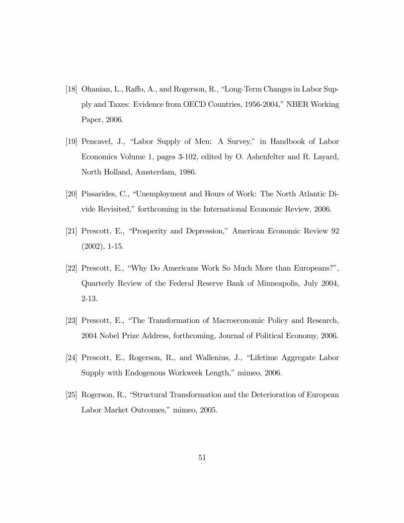
a relatively high labor supply elasticity. One critique of these exercises is that the
assumed labor supply elasticity of the stand-in household is much larger than that
implied by most estimates based on micro data. Specifically, if the labor supply
elasticity of the stand-in household was instead set to standard estimates based
on micro data, then it is no longer the case that taxes account for a large share
of differences in market work between the US and continental Europe.1 In this
paper we argue that this critique is misplaced.
To make this point, we develop an overlapping generations model that repli-
cates the salient features of life cycle labor supply, and then use this model to
analyze how tax and transfer policies affect hours of work in the steady state. In
this framework we can carry out both standard micro data estimation exercises
based on life cycle variation for prime aged workers, as well as standard macro es-
timation based on variation in aggregates across steady states. Our main findings
are twofold. First, macro elasticities are virtually unrelated to micro elasticities,
and second, macro elasticities are large. In particular, for micro elasticities that1Alesina et al (2005) is a recent example where this critique is put forward.
1
vary by a factor 25, ranging from .05 to more than 1.25, the corresponding macro
elasticities are in the range of 2.25− 3.0.
Our model builds on the earlier work of Prescott et al (2006) on lifetime labor
supply by imbedding it into a life cycle setting. Like them, we focus on the
importance of non-linearities in the mapping from time at work to labor services
provided. This feature gives rise to equilibrium allocations in which workers choose
time allocations in which both the extensive and intensive margins are operative,
i.e., a worker chooses both what fraction of his or her life to devote to employment,
and what fraction of his or her period time endowment to devote to work while
employed. By imbedding this analysis into a life cycle model we are able to
generate standard life cycle profiles for hours of work—including the fact that
hours drop discontinuously to zero at older ages. This allows us to reproduce
micro estimates based on life cycle variation for prime aged workers.
In addition to reconciling micro and macro tax elasticities, our life cycle model
delivers two additional predictions relative to earlier analyses based on stand-in
household models, both of which are also corroborated by the cross-country data.
First, our model predicts that increases in the size of tax and transfer policies
imply less time devoted to work both in terms of employment to population ratios
and hours of work per person in employment. Second, our model implies that
differences in employment to population ratios are dominated by differences among
young and old individuals.
Our results are related to those in a recent paper by Chang and Kim (2006).
They study a model in which individuals are subject to idiosyncratic shocks to
2
wages, can self-insure through saving but have no access to insurance markets,
and in which labor is indivisible, so that the supply decision consists solely of a
decision at the extensive margin. Similar to our result, they find that in their
model, micro and macro elasticities need not be the same, and that macro elas-
ticities can be significantly larger. While we view our study as complementary
to theirs, there are several important differences that distinguish the two studies.
First, our model is a life cycle model and hence can explicitly connect to micro
estimates based on life cycle variation. Second, our analysis allows for variation
along both the intensive and extensive margin. Not only does this allow one to
better match the cross-country differences in hours of work, but we show that
there is an important interaction between intensive and extensive margins: less
movement on the extensive margin necessarily implies more adjustment on the
intensive margin. Third, and related to this point, Chang and Kim argue that
increases in heterogeneity in the steady state cross-sectional distribution of wages
imply a large reduction in implied macro elasticities. We find that having an
operative intensive margin reduces the quantitative impact of this effect.
An outline of the paper follows. Section 2 presents the model, and Section 3
develops a simple characterization of steady-state life cycle labor supply. Section 4
considers the effects of tax and transfer programs on the equilibrium, and considers
the relationship between micro and macro elasticities. Section 5 considers some
extensions of the analysis, and section 6 concludes.
3
2. Model and Equilibrium
The model is purposefully specialized along several dimensions in order to best
highlight those relationships that are the focus of our analysis. We consider a
continuous time overlapping generations framework in which a unit mass of iden-
tical, finitely lived individuals is born at each instant of time t. Continuous time
is convenient for our analysis because we will study the endogenous determina-
tion of the length of working life, and continuous time allows us to model this
as a continuous choice variable. We normalize the length of the lifetime of each
agent to one and assume that each individual is endowed with one unit of time
at each instant. Letting a denote age, individuals have preferences over paths for
consumption (c(a)) and hours worked (h(a)) given by:
Z 1
0
U(c(a), 1− h(a))da (2.1)
where U is twice continuously differentiable, strictly increasing in both arguments
and strictly concave. Note that we assume that individuals do not discount future
utility.2
We assume that labor is the only factor of production, and write the aggregate
production function as:
Y (t) = L(t) (2.2)
where L(t) is aggregate input of labor services. A key feature of our model is2This is done purely for convenience to allow us to focus on a zero interest rate steady state.
From the perspective of hours worked, interest rates and discount factors serve primarily to tiltthe life cycle profile.
4
the mapping from hours of work into labor services, which is described by two
functions, e(a) and g(h). In particular, we assume that if an individual of age
a devotes h units of time to market work then it will yield l = e(a)g(h) units
of labor services. The function e(a) is standard in the life cycle labor supply
literature–it represents exogenous life cycle variation in individual productivity.
This feature will be the driving force behind the variation in hours worked during
that part of the life cycle in which an individual is employed. In a later section we
will also consider variation in the disutility of work and show how it can play a
similar role. We assume that the function e(a) is single peaked, twice continuously
differentiable, and has zero derivative only at its global maximum, i.e., that it has
no flat spots.
Following Prescott et al (2006), the function g(h) is somewhat nonstandard,
but plays a critical role in the analysis. A standard assumption in the literature
is that g is linear with slope equal to one, so that for a worker of a given age,
labor services are linear in hours of work. We assume that g is continuous, and
increasing, with g(0) = 0, but we depart from the assumption of linearity. In
particular, we assume that there is a value h with 0 < h < 1 such that g is strictly
concave over the region [h, 1], but not over the region [0, 1]. The function g(h)may
be convex over the region [0, h]. One justification for the initial convex region is
fixed costs associated with getting set up for a job and costs associated with being
supervised. This is consistent with the observation that firms do not consider part-
time workers for many positions.3 The justification for the strictly concave region3Our analysis emphasizes non-linearities in the mapping from hours worked to labor services
provided. Similarly, one could allow for the possibility of non-linearities in the mapping from
5
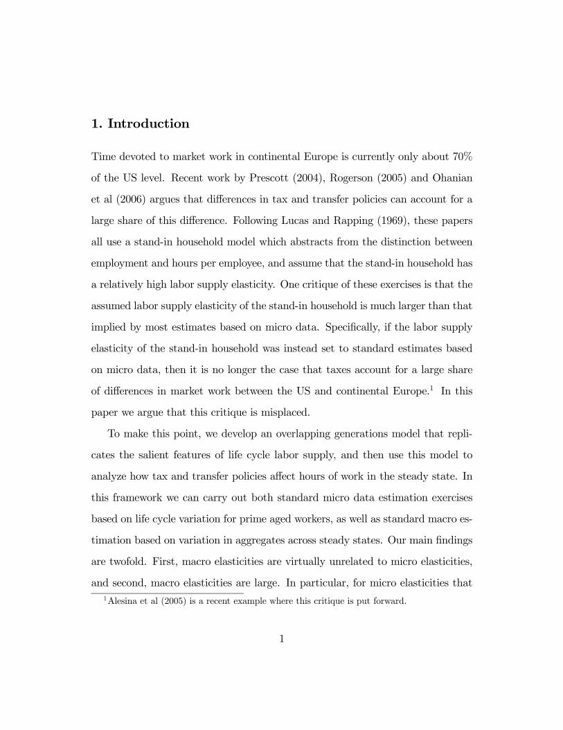
is fatigue. Figure 1 shows one possible g that satisfies these properties.
0 0.2 0.4 0.6 0.8 10
0.005
0.01
0.015
0.02
0.025
0.03
0.035
0.04
0.045
Time Devoted to Market Work
Labo
r Ser
vice
s
Figure 1: The g(h) Function
It is important to note the significance of the assumed properties of the func-
tion g(h). These properties serve to generate a nonconvexity in the aggregate
technology set for this economy. In a static setting with homogeneous agents,
this nonconvexity implies that it may be optimal to randomly select a fraction of
workers to work positive hours and have the remaining workers work zero hours.
Loosely speaking, in such a setting this feature of technology can serve to endo-
genize the length of working time in a model of indivisible labor. Generalizing
this homogeneous worker model to a dynamic setting with no discounting and no
life cycle effects, Prescott et al (2006) showed that if time is continuous, optimal
allocations take the form of a constant working time for employed workers, and a
constant fraction of individuals employed at each instant. Importantly, such an
leisure time to the leisure services.
6
allocation can be implemented as an equilibrium without lotteries, since individu-
als can choose the fraction of their lifetime that they work and use asset markets
to smooth consumption in the face of an uneven income stream.
In the next section we show that in our overlapping generations model with
life cycle effects, this feature can give rise to equilibria in which there is a well-
defined notion of a working life—individuals will begin work at a particular age, and
work continuously until retirement, at which point hours of work drop to zero.
Moreover, the events of entering and leaving the labor force are discontinuous
events, in the sense that hours of work jump discontinuously at these two points.
In particular, hours of work do not gradually decrease to zero prior to retirement.
2.1. Equilibrium
We consider the following market structure. We assume that at time zero there
are markets for labor services and consumption at all future dates. Let w(t) and
p(t) denote the paths for prices in these two markets. We assume competitive
behavior in all markets. If a given individual is alive at two dates t and t0, this
market structure implicitly allows an individual to borrow or lend resources across
these two dates at the gross interest rate p(t)/p(t0). Given that the aggregate
production function is linear in labor services, competitive equilibrium necessarily
implies that w(t) = p(t) at each t.
Our analysis will focus on steady state equilibria associated with this market
structure. As is well known, overlapping generations models can give rise to
multiple steady state equilibria. For our economy, one can show that there is
7
always one steady state equilibrium in which p(t) is constant, i.e., a steady state
with a zero interest rate. Given that we assumed no discounting, this steady
state will dominate any other steady state, and thus it is natural to focus on it.
One potential problem is that there might not be any equilibrium that converges
to this steady state without government intervention. In particular, it may be
necessary for the government to issue debt in order to achieve the zero interest
rate steady state. In the analysis that follows we will assume that if necessary,
the government follows a policy that results in this steady state equilibrium being
reached, and will therefore focus on the zero interest rate steady state equilibrium.
What matters for our subsequent analysis is not that the interest rate is equal to
zero, but rather that the interest rate is constant across steady states in the face
of the labor policies that we consider.4
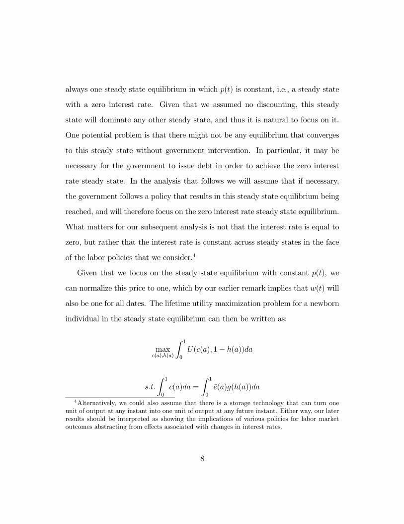
Given that we focus on the steady state equilibrium with constant p(t), we
can normalize this price to one, which by our earlier remark implies that w(t) will
also be one for all dates. The lifetime utility maximization problem for a newborn
individual in the steady state equilibrium can then be written as:
maxc(a),h(a)
Z 1
0
U(c(a), 1− h(a))da
s.t.
Z 1
0
c(a)da =
Z 1
0
e(a)g(h(a))da
4Alternatively, we could also assume that there is a storage technology that can turn oneunit of output at any instant into one unit of output at any future instant. Either way, our laterresults should be interpreted as showing the implications of various policies for labor marketoutcomes abstracting from effects associated with changes in interest rates.
8
It is of interest to first consider the special case in which e(a) is constant over
an individual’s life. This case was studied by Prescott et al (2006), and they show
that the solution for h(a) can take one of two forms. One possibility is that h(a)
is positive for all a, in which case the solution for h(a) is unique and has h(a)
constant for all a. The other possibility is that h(a) is equal to zero for some a (in
a set with positive measure). In this case there is a continuum of solutions for h(a),
but each characterized by the same two values: f , the fraction of the individual’s
life spent in employment, and h, the time devoted to work at any instant in which
the individual is employed. That is, the solution pins down hours of work when
employed and total hours supplied over the lifetime, but the timing of work is
indeterminate.5 Of course, in steady state equilibrium, it is necessary that the
pattern of hours worked across individuals be such as to yield constant aggregate
hours at each point in time.
We now return to the case in which e(a) is not constant. The next proposition
states a very simple property of the optimal solution to this problem.
Proposition 1: The optimal solution for h(a) has a reservation property. In
particular, there exists a value e∗ such that h(a) > 0 if e(a) > e∗ and h(a) = 0 if
e(a) < e∗. Moreover, the solution for h(a) is unique.6
Proof: Suppose the solution does not have the reservation property, i.e., sup-
pose there are ages a1 and a2 such that h(a1) > 0, h(a2) = 0 and e(a2) > e(a1).
Consider the alternative solution in which the individual switches the hours of5The idea that theory predicts only the total time spent in employment and not the timing
of employment was first noted by Mincer (1962) in his study of labor supply by married women.6Formally, this result can be violated on a set of measure zero. For simplicitly, we will
abstract from this issue in both the statement of propositions and our proofs.
9
work and consumptions at these two ages. The lifetime utility of work is identical
under these two scenarios, but the alternative scenario generates higher lifetime
income, implying that consumption can be increased, thereby leading to higher
lifetime utility. It follows that there is a reservation value e∗. Given that the
timing of work is pinned down by the reservation value, and that e(a) has no flat
spots aside from at its maximum, it follows from standard arguments that the
optimal solution for h(a) is unique. //
Relative to the case in which e(a) is constant, we see that allowing this function
to vary over the life cycle serves to eliminate the indeterminacy.7 Intuitively,
making individual productivity vary over time breaks the indeterminacy regarding
the timing of labor supply, since the individual prefers to work when productivity
is relatively high. The above result does not rule out the possibility that e∗ = 0,
in which case all individuals will work positive hours in the market at all points
during their lives. But independently of whether hours are not always positive,
this result coupled with our assumption on the profile e(a) implies that there is a
unique starting time for employment and a unique stopping time for employment
(though one or both of these could still be at a corner). In particular, if we define
follows that the individual will begin work at age A1, and work continuously until
reaching age A2, at which point the individual will retire and not devote any time
to market work from this age on.
The same logic which implies that the individual should work when produc-7Mulligan (2001) notes this same property in a model with indivisible labor.
10
tivity is highest also implies that conditional on working, hours of work should be
increasing in e(a). In particular, we have the following proposition.
Proposition 2: Let h∗(a) be the optimal solution for hours of work over the
life cycle. Let a1 and a2 be distinct ages for which h(a) > 0. Then e(a1) > e(a2)
implies h(a1) > h(a2).
Proof: Let c(a) be the optimal profile for consumption. Assume by way of
contradiction that e(a1) < e(a2) and h(a1) ≥ h(a2). The assumed profiles cannot
be utility maximizing, since by switching the values of c and h at ages a1 and a2,
lifetime utility and expenditure are unchanged, while income increases, thereby
allowing for higher utility .//
3. Solving the Individual’s Problem
Although the analysis thus far has not made any specific assumptions about func-
tional forms, for the analysis that follows we will impose some additional as-
sumptions. In particular, we will assume that preferences are separable between
consumption and leisure:
U(c, 1− h) = u(c)− v(h) (3.1)
where the function u(c) is twice continuously differentiable, strictly increasing
and strictly concave, and v(h) is assumed to be twice continuously differentiable,
strictly increasing and strictly convex.
Given no discounting, a zero interest rate, separable utility and strict concavity
11
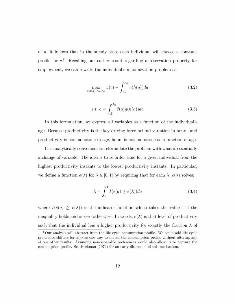
of u, it follows that in the steady state each individual will choose a constant
profile for c.8 Recalling our earlier result regarding a reservation property for
employment, we can rewrite the individual’s maximization problem as:
maxc,h(a),A1,A2
u(c)−Z A2
A1
v(h(a))da (3.2)
s.t. c =
Z A2
A1
e(a)g(h(a))da (3.3)
In this formulation, we express all variables as a function of the individual’s
age. Because productivity is the key driving force behind variation in hours, and
productivity is not monotone in age, hours is not monotone as a function of age.
It is analytically convenient to reformulate the problem with what is essentially
a change of variable. The idea is to re-order time for a given individual from the
highest productivity instants to the lowest productivity instants. In particular,
we define a function e(λ) for λ ∈ [0, 1] by requiring that for each λ, e(λ) solves:
λ =
Z 1
0
I(e(a) ≥ e(λ))da (3.4)
where I(e(a) ≥ e(λ)) is the indicator function which takes the value 1 if the
inequality holds and is zero otherwise. In words, e(λ) is that level of productivity
such that the individual has a higher productivity for exactly the fraction λ of8Our analysis will abstract from the life cycle consumption profile. We could add life cycle
preference shifters for u(c) as one way to match the consumption profile without altering anyof our other results. Assuming non-separable preferences would also allow us to capture theconsumption profile. See Heckman (1974) for an early discussion of this mechanism.
12
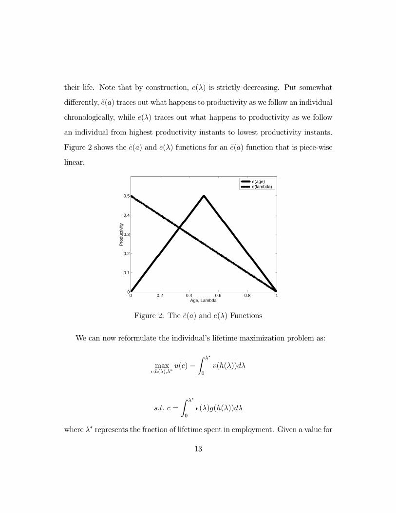
their life. Note that by construction, e(λ) is strictly decreasing. Put somewhat
differently, e(a) traces out what happens to productivity as we follow an individual
chronologically, while e(λ) traces out what happens to productivity as we follow
an individual from highest productivity instants to lowest productivity instants.
Figure 2 shows the e(a) and e(λ) functions for an e(a) function that is piece-wise
linear.
0 0.2 0.4 0.6 0.8 10
0.1
0.2
0.3
0.4
0.5
Age, Lambda
Prod
uctiv
ity
e(age)e(lambda)
Figure 2: The e(a) and e(λ) Functions
We can now reformulate the individual’s lifetime maximization problem as:
maxc,h(λ),λ∗
u(c)−Z λ∗
0
v(h(λ))dλ
s.t. c =
Z λ∗
0
e(λ)g(h(λ))dλ
where λ∗ represents the fraction of lifetime spent in employment. Given a value for
13
λ∗ it is straightforward to back out the implied values for A1 and A2. If solutions
for both are interior then they solve:
e(A1) = e(A2) = e(λ∗)
Using the budget equation to substitute for c in the objective function, this
problem can be reduced to finding a value of λ∗ and an hours profile h(λ) for
0 ≤ λ ≤ λ∗. Assuming that the solution for λ∗ is interior9 and that h(λ) < 1 for
all λ, we obtain the following first order conditions for λ∗ and h(λ) for 0 ≤ λ ≤ λ∗:
v(h(λ∗))
u0(R λ∗
0e(λ)g(h(λ))dλ)
= e(λ∗)g(h(λ∗)) (3.5)
v0(h(λ))
u0(R λ∗
0e(λ)g(h(λ))dλ)
= e(λ)g0(h(λ)) (3.6)
Both of these equations have a standard interpretation: labor is adjusted on
each margin until the marginal rate of substitution between leisure and consump-
tion is equal to the marginal product of labor along each margin, though only the
second equation corresponds to the standard textbook model of labor supply. For
the case of hours worked while employed, the relevant margin is how many hours
to work at a given instant, so that the marginal disutility associated with an ad-
ditional hour is equal to v0(h(λ)), while the marginal product associated with an
additional hour is e(λ)g0(h(λ)). For the case of adjusting the length of working
life, the marginal disutility associated with increasing the fraction of life spent in9Note that the solution for λ∗ is interior as long as one of the Ai’s has an interior solution.
14
employment is v(h(λ∗)), while the marginal product associated with increasing
the fraction of life spent in employment is e(λ∗)g(h(λ∗)).
Although solving the maximization problem requires finding the value λ∗ and
the entire h(λ) profile, we will show that the problem can be reduced to finding
two values: λ∗ and h(0). To see why this is the case, note that equation (3.6)
implies that along the optimal profile h(λ), we must have:
v0(h(λ))
e(λ)g0(h(λ))= constant for all λ ∈ [0,λ∗] (3.7)
If h(λ) lies in the region in which g is concave, then the strict convexity of v
implies that the left hand side of this equation is strictly increasing in h(λ). In
this case it then follows that if h(0) is known, the entire h(λ) profile is uniquely
determined. Additionally, given the monotonicity property just mentioned, an
increase in h(0) leads to an upward shift of the entire h(λ) profile. A potential
problem with this argument is that h(λ) does not necessarily lie in the region
where g is concave. However, although one cannot guarantee that h(λ) lies in
the region where g is concave, the second order conditions for the maximization
problem nonetheless do require that at an optimum, the left-hand side of equation
(3.7) is strictly increasing in h. Loosely speaking, although the optimum need not
occur at a point at which g is concave, the convexity of v in hours must dominate
the lack of concavity in g.10
10More formally, if one reformulates the problem as having the worker choose how many unitsof labor services to offer at each instant, the relevant disutility over labor services can be writtenas v(g−1( l
e(λ))) and the second order condition requires that v be convex at the optimum choiceof labor services. This condition implies that the left hand side of equation (3.7) is strictlyincreasing in h.
15
Having established that solving the consumer’s problem can be reduced to
finding optimal values for h(0) and λ∗, we next show that the equilibrium can
be described as the intersection of two curves in h(0)− λ∗ space, one of which is
(at least locally) upward sloping, and the other of which is (globally) downward
sloping. To derive the upward sloping relationship, we note that dividing the two
first order conditions by each other, evaluating at λ = 0, and rearranging, one
obtains:
v0(h(0))
e(λ)g0(h(0))=
v(h(λ∗))
e(λ∗)g(h(λ∗))for all λ ∈ [0,λ∗] (3.8)
To see that this expression implies a relationship between h(0) and λ∗ simply note
that given a value of h(0) we can infer the profile h(λ) using equation (3.7). Given
this profile, we then evaluate the right hand side at each point of the profile to find
a value of λ such that equation (3.8) holds. We now show that in a neighborhood
of the optimal solution, the relationship between h(0) and λ∗ is increasing.
Proposition 3: In a neighborhood of the optimal solution, equation (3.8) defines
an increasing relationship between h(0) and λ∗.
Proof: To prove this we establish three properties. First, the left-hand side
of equation (3.8) is strictly increasing in h(0). Second, given an optimal profile
h(λ), the right hand side of equation (3.8) is increasing in λ. Third, the marginal
effect of an increase in h(0) on the right hand side of equation (3.8) evaluated at
the optimal λ∗ is zero. Combining these three properties, the result necessarily
follows. Since the first property has already been noted, it remains to establish
the second and third properties.
16
To establish the second property we simply take the derivative of the right
hand side of equation (3.8) with respect to λ and evaluate it at λ = λ∗. This
yields:
− e0(λ∗)
e(λ∗)2v(h(λ∗))
g(h(λ∗))+
1
e(λ∗)
g(h(λ∗))v0(h(λ∗))− v(h (λ∗)) g0(h(λ∗))g(h(λ∗))2
h0(λ∗) (3.9)
However, noting that equation (3.7) holds for λ = λ∗, it follows that the second
term is necessarily zero, and that the sign of this expression is therefore simply the
sign of −e0(λ∗), which is necessarily positive by construction of the e(λ) function.
To establish the third property, we simply differentiate the right hand side of
equation (3.8) evaluated at λ∗ with respect to h(0), and evaluate at the optimal
value of h(0). This gives:
1
e(λ∗)
g(h(λ∗))v0(h(λ∗))− v(h (λ∗)) g0(h(λ∗))g(h(λ∗))2
∂h(λ∗)/∂h(0) (3.10)
Since the middle term of this expression is equal to zero by equation (3.7), it
follows that this derivative is zero.
Having established the three properties, the result follows.//
This upward sloping relationship is intuitive. Equation (3.8) has the interpre-
tation that the marginal disutility per unit of additional output is equal across the
two margins h(0) and λ∗. Since this marginal disutility is increasing along both
margins, if more time is devoted to market work along one margin, then more
time must be devoted to market work along the other margin as well, in order
for the two disutilities to be equated. We will call the curve that captures this
17
relationship the optimal composition of work curve.
Similarly, given a value for h(0) and the implied profile for h(λ), equation (3.6)
evaluated for λ = 0 gives:
e(0)g0(h(0))
v0(h(0))=
1
u0(R λ∗
0e(λ)g(h(λ))dλ)
(3.11)
We now show that this expression produces a negative relationship between λ∗
and h(0). To see this, note first that holding λ∗ constant, the left hand side of
equation (3.11) is decreasing in h(0), while the right hand side is increasing in h(0),
since an increase in h(0) shifts the entire h(λ) profile upward and g is an increasing
function. Second note that holding h(0) constant, the right hand side is increasing
in λ∗. It follows immediately that this equation describes a negative relationship
between h(0) and λ∗. This relationship is also intuitive. Equation (3.11) has the
interpretation that the marginal rate of substitution between consumption and
leisure be equated to the marginal product of time devoted to market work. But
since an increase in time devoted to market work along one margin leads to higher
consumption and therefore raises the marginal rate of substitution, it leads to less
time devoted to market work along the other margin. Put somewhat differently,
from the perspective of generating income, the two margins are substitutes. We
will call the curve that captures this relationship the optimal volume of work curve.
Combining these results, it follows that one can represent the problem of solv-
ing for the optimal hours profile h(λ) and the optimal time spent in employment,
λ∗, as the intersection of two curves in h(0) − λ∗ space, with one curve being
upward sloping and the other curve being downward sloping. Figure 3 depicts the
18
situation.
0 0.2 0.4 0.6 0.8 10
0.1
0.2
0.3
0.4
0.5
0.6
0.7
0.8
0.9
Fraction of Life in Employment
Hou
rs a
t Pea
k Pr
oduc
tivity
Optimal Volume of Work
Optimal Composition of Work
igure 3: Equilibrium Determination of h(0) and λ∗
This diagrammatic representation will be useful when we consider the effect
of tax policies.
4. Tax Policies and Labor Supply Elasticities
In this section we consider how a tax and transfer policy affects the equilibrium
hours worked profiles for individuals, both analytically as well as quantitatively.
In particular, similar to the tax and transfer policy studied by Prescott (2004),
we assume that the government taxes all labor income at the constant rate of τ
and uses the tax revenues to fund an equal lump-sum transfer T at each instant
to all individuals, subject to a balanced budget constraint at each instant of time.
In steady state, tax revenues will be constant and hence the lump-sum transfer
will be constant as well.
19
4.1. Analytic Results
Given this policy, the individual lifetime maximization problem becomes:
maxc,h(λ),λ∗
u(c)−Z λ∗
0
v(h(λ))dλ
s.t. c = (1− τ)
Z λ∗
0
e(λ)g(h(λ))dλ+ T
The first order conditions for this problem are:
v(h(λ∗))
u0((1− τ)R λ∗
0e(λ)g(h(λ))dλ+ T )
= (1− τ)e(λ∗)g(h(λ∗)) (4.1)
v0(h(λ))
u0((1− τ)R λ∗
0e(λ)g(h(λ))dλ+ T )
= (1− τ)e(λ)g0(h(λ)) (4.2)
Noting that the balanced budget rule for the government implies:
τ
Z λ∗
0
e(λ)g(h(λ))dλ = T (4.3)
the two previous equations can be written as:
(1− τ)e(λ∗)g(h(λ∗))
u0(R λ∗
0e(λ)g(h(λ))dλ)
= v(h(λ∗)) (4.4)
(1− τ)e(λ)g0(h(λ))
u0(R λ∗
0e(λ)g(h(λ))dλ)
= v0(h(λ)) (4.5)
20
As before, equation (4.5) implies that along the optimal profile, e(λ)g0(h(λ))/v0(h(λ)
will be constant, implying that one can infer the entire h(λ) profile from the value
of h(0). Moreover, using this fact and proceeding as before, one can show that
equilibrium can be summarized by the following two relations, each of which de-
scribes a relationship between h(0) and λ∗:
v0(h(0))
e(0)g0(h(0))=
v(h(λ∗))
e(λ∗)g(h(λ∗))(4.6)
(1− τ)e(0)g0(h(0))
v0(h(0))=
1
u0(R λ∗
0e(λ)g(h(λ))dλ)
(4.7)
The first equation is the same expression as in the zero tax case, while the second
expression now contains a term (1− τ). It is straightforward to establish that an
increase in τ implies a lower value of λ∗ for a given value of h(0). It follows that the
optimal composition of work curve is unaffected by taxes, while an increase in taxes
shifts the optimal volume of work curve downward. The following proposition is
then immediate:
Proposition 4: An increase in τ leads to a decrease in λ∗ and a downward shift
in h(λ) for all λ ∈ [0,λ∗].
Proof: Follows immediately from Figure 3, and the previous result concerning
the effect of τ on the two curves.//
It is interesting to contrast this result with that which obtains in the case
where the e(λ) profile is flat. In this case an increase in taxes leads to a lower
fraction of life spent in employment but no change in the hours profile.
21
4.2. Quantitative Results
In this subsection we report the results of some numerical simulations regarding
the effects of taxes on hours of work.
4.2.1. Calibration
For these calculations we adopt the following functional forms:
u(c) = log(c), v(h) = αh1+γ
1 + γ, (4.8)
g(h) = (h− h) for h ≥ h, 0 otherwise, e(λ) = e0 − (e0 − e1)λ.
The function u(c) is chosen in order to be consistent with balanced growth in a
setting with technological progress, though we abstract from growth here. The
choice of v(h) is standard and is convenient since the parameter γ determines the
elasticity of hours with respect to the tax rate in a standard labor supply model
in which g(h) is identically equal to one. Our choice for the function g is dictated
by parsimony. The exact shape of g for h ≤ h is not important as long as the
individual chooses to work h ≥ h, and so we set g = 0 in this region. We also
abstract from fatigue effects in this specification. The assumed functional form
for e(λ) implies a linear productivity profile, with initial productivity e0 and final
productivity e1. While the data suggests that linearity is not necessarily a good
assumption for this profile, we adopt it because it permits a parsimonious way
to investigate the importance of the slope of this profile in affecting how hours
and employment respond to changes in taxes. It is easy to show that with our
22
assumption on preferences, specifically that utility from consumption is log(c),
the solution for h(λ) is unaffected by a proportional shift in the e(λ) profile, so
that we can normalize e0 to one with no loss in generality.
Given these functional forms, we will investigate how the parameter γ matters
for some properties of the life cycle profile and how this profile responds to tax and
transfer policies. For each value of γ we will choose values for the three parameters
α, h, and e1 so as to match three target values. The first target is the fraction of
life spent in employment. If we interpret our model as representing an adult life
span of 60 years, then a working life of approximately 40 years implies a target
value for λ∗ of .67. If the peak workweek for employed workers over the life cycle is
around 45 hours per week and individuals have roughly 100 hours of discretionary
time per week, then recalling that we normalized the time endowment to one at
each instant, the target value for h(0) is .45. Lastly, given a target value for λ∗,
the value of e1 will influence the range of productivities over the life cycle, and
hence the range of hourly wages. We choose a value for e1 so that hourly wages
at their peak are twice as large as hourly wages at their lowest point. Because the
results that we report below are very robust to changes in these values, we do not
want to focus on justifying these exact values.
It is important to point out that some care needs to be taken in matching up
wages in the model with wages in the data. In the model, the wage per unit of
labor services, which we denoted by w, is equal to one at all points in time. But
wages in the data are measured as labor earnings per hour of work, and so we
compute this same measure in our model. We denote this wage rate as wh, where
23
the superscript h denotes that we are measuring wages per hour of work. If the
function g were identically equal to one then earnings per hour of work in the
model would be exactly equal to e(λ) and hence the range of wages over the life
cycle would be exactly equal to e(0)/e(λ∗). But since the function g is non-linear,
this no longer holds. The range of wages over the life cycle in our calibrated model
is given by:wh(0)
wh(λ∗)=
e(0)g(h(0))/h(0)
e(λ∗)g(h(λ∗))/h(λ∗)(4.9)
While the hourly wage ratio is influenced by e(0)/e(λ∗), these values are no longer
identical. Nonetheless, one can choose e1 such that this ratio is equal to 2 in the
benchmark calibration.
In calibrating the model, we also assume a tax rate of .3, which corresponds
to the average effective tax on labor income in the US in recent years. Having
calibrated the model, we will then examine what happens to equilibrium hours if
the tax rate were increased to .5, which corresponds to the average effective tax
on labor income in several economies in continental Europe in recent years.11
4.2.2. Micro Elasticities
Before reporting the results of the change in tax and transfer policies, it is of
interest to examine some features of the calibrated benchmark economies. Given
a value of γ and the calibration procedure just described, the model will generate11Several authors have produced estimates of effective tax rates for various countries, including
Mendoza et al (1994), Prescott (2004) and McDaniel (2006). While there are small differences inmethodology across studies, the 20% differences between the US and countries such as Belgium,France, Germany and Italy is a robust finding.
24
a life cycle profile for hours worked, h(λ), and hourly wages, wh(λ). We generate a
panel life cycle data set for hourly wages and hours worked by choosing 67 equally
spaced values of λ, running from 0 to .66 and evaluating the two functions h(λ)
and wh(λ) at these points. Note that all of the data points in the sample are times
at which individuals are employed. Using t to index the data points for a given
individual, as is standard in the labor supply literature we take this data and run
the regression:
log(ht) = b0 + b1 log(wht ) + εt (4.10)
The resulting parameter estimate b1 is the so-called micro Frisch labor supply
elasticity.
Table 1 shows the estimated values of b1 for our benchmark calibrated model
for four different values of γ : .5, 1, 2, and 10.
Table 1
Estimated Micro Frisch Elasticities
γ = .5 γ = 1 γ = 2 γ = 10
1.29 .59 .28 .05
The table shows that higher values of γ are associated with lower Frisch elas-
ticities, though note that the nonlinearity of the g function implies that the Frisch
elasticity is not equal to 1/γ.12 There is a voluminous literature that has esti-
mated Frisch elasticities. The estimates are typically found to be smaller for males
than for females, with the value for males typically less than .3, and values for12In particular, the nonlinearity of g implies that higher hours imply higher hourly wage rates,
thereby lowering the estimated elasticity relative to a standard model.
25
females perhaps as large as 1.13 One could use a target value for this elasticity to
calibrate the value of γ, but as we will see, it turns out to be quite interesting to
simply consider each of these four cases.
4.2.3. Tax and Transfer Policies
We now turn to the evaluation of tax and transfer policies. For each of the four
different calibrated economies (one for each of the four values for γ in Table 1),
we consider what happens to the steady state hours profile if we increase the tax
rate on labor income from .3 to .5, assuming that the proceeds fund a uniform
lump-sum transfer to all individuals subject to a balanced budget constraint at
each point in time. With our functional forms, one can show that such a tax
causes a proportional shift in the hours profile, conditional on being employed. It
follows that one can summarize the shift in the hours profile by simply reporting
the shift in h(0). For each economy we compute the values of aggregate hours
(H), fraction of life spent in employment (λ∗), and peak hours worked over the
life cycle (h(0)), all relative to the values in the benchmark calibrated economy
with τ = .3. Table 2 reports the results.13Classic references for estimates of Frisch elasticities using micro panel data are MaCurdy
(1981) for men and Heckman and MaCurdy (1980) for women. See the survey of Pencavel (1986)for an extensive list of other contributions and the more recent survey of Blundell and MaCurdy(1999) for additional discussion. Heckman (1993) notes the importance of the extensive andintensive margins in interpreting most studies.
26
Table 2
Relative Outcomes for τ = .5
γ H λ∗ h(0)
.50 .777 .857 .856
1.00 .784 .825 .918
2.00 .788 .808 .956
10.00 .790 .794 .991
Several features are worth noting. First, note that the implied change in ag-
gregate hours worked is large in all four cases—more than 20%. Second, despite
the dramatic differences in estimated Frisch elasticities in the four economies—
a factor 25 difference between the highest and lowest—the changes in aggregate
hours worked are essentially constant across the four different economies. Third,
although the value of γ has virtually no effect on the change in aggregate hours
worked, it has very significant effects on how the change in aggregate hours is
broken down into changes in working life versus changes in hours worked while
employed. In analyzing this decomposition, it is important to note that the rela-
tive change in h(0) is a measure of the change in total hours due to changes in the
h profile holding λ∗ constant, since as noted earlier, the h profile shifts propor-
tionately, and for a given λ∗, a proportionate shift in the profile shifts aggregate
hours by the same amount. However, it is not true that a shift in λ∗ leads to
a proportionate shift in aggregate hours, since as λ∗ decreases the marginal em-
ployment episodes that are lost represent fewer hours of work. In any case, when
γ = .50 the downward shift in the hours profile accounts for over 60% of the total
27
decrease in hours, while when γ = 10 this downward shift accounts for less than
5% of the shift.
There are two additional implications of the model not reported in Table 2
that are also of interest. Because time devoted to work and labor services are
not proportional in our model, it is of interest to contrast the effects of taxes
on aggregate labor services with the effect on aggregate time devoted to work.
Additionally, although changes in taxes do not affect technology in our analysis,
they can affect productivity measures such as output per hour because of the
difference between labor services and time devoted to market work. Note that
there are two opposing effects of higher taxes on productivity per hour in our
model. On the one hand, the decrease in hours is concentrated among lower
productivity workers since this is where the extensive margin is operative, which
would lead to higher output per hour in the high tax economy. On the other
hand, higher taxes shift the hours profile down, thereby lowering the ratio of labor
services to hours, and leading to lower productivity. The importance of these two
effects is influenced by the relative size of adjustment along the intensive and
extensive margin, and hence by the value of γ. However, it turns out that these
effects are relatively small in our numerical examples. For all four economies the
increase in taxes is associated with a drop in output per hour, but the decrease is
less than 1%, and ranges between .9% and .6% as γ is varied from 10 to .5.
While Table 2 contrasted outcomes for just two different tax rates for a range
of values of γ, we note that the effects are very close to linear in the tax rate. For
completeness, Table 3 presents results for a range of tax rates for the specification
28
that corresponds to γ = 2.
Table 3
Tax Effects (γ = 2, all values relative to τ = .30)
τ = .35 τ = .40 τ = .45 τ = .50 τ = .55 τ = .60
H .950 .899 .844 .788 .729 .665
λ∗ .956 .910 .860 .808 .752 .692
h(0) .990 .979 .968 .956 .945 .933
4.2.4. Comparison With a Stand-In Household Economy
The model economy that we have studied is not a single agent economy, in the
sense that at any point in time there are many different types of individuals alive.
However, it is interesting to ask what one might infer about labor supply if one
were to interpret the outcomes generated by the tax changes in our model by
using a standard static stand-in household model. In particular, consider a static
economy with a single agent, with preferences given by:
log(c)− µ h1+θ
1 + θ(4.11)
There is a linear technology in this economy that can turn one unit of time into
one unit of consumption:
c = h
and there is a government that taxes labor at the constant proportional rate of τ
and uses the proceeds to fund a lump-sum transfer to the representative agent.
29
Faced with the information in Table 2, we ask what an economist using this
model to interpret the hours differences would conclude about the parameter θ
that dictates the labor supply elasticity for the stand-in household in this economy.
Standard calculations for this economy lead to the following expression for hours
of work in terms of taxes:
h = [1− τ
µ]1/(θ+1) (4.12)
If we let hi denote the hours that correspond to a country with tax rate τ i, for
i = 1, 2, then using the above expression to interpret data on taxes and hours of
work leads to the following expression for θ :
θ =log(1− τ 1)− log(1− τ 2)
log(h1)− log(h2)− 1 (4.13)
Applying this expression to the four calibrated economies, we obtain the results
shown in Table 4:
Table 4
Implied Values for θ
γ = .5 γ = 1 γ = 2 γ = 10
.33 .38 .41 .43
The associated Frisch elasticities, given by 1/θ, range from 2.3 to 3, despite the
fact that the Frisch elasticities inferred from micro data range from .05 to 1.25.14
14One can show that our steady equilibrium corresponds to the allocation that maximizes anequal weighted sum of individual utilities. It follows that one can derive an analytic expressionfor preferences of the stand-in household.
30
The above calculation shows that a static stand-in household model with a
fairly high labor supply elasticity can reproduce the steady state effects of taxes
on aggregate hours found in the life cycle model studied earlier. It is also of inter-
est to ask whether the welfare implications of tax changes are similar across the
two specifications. Our measure of welfare is the percent increase in lifetime con-
sumption required to make households living in the high tax economy indifferent
to living in the low tax economy. It turns out that the answers are remarkably
similar in the life cycle and stand-in household models. For example, in the γ = 1
economy the welfare cost of the higher tax system is 10.7% of consumption, while
in the corresponding stand-in household model the welfare cost is 10.4% of con-
sumption.
4.2.5. The Role of g(h)
The above results indicate that in our life cycle economy, micro labor supply
elasticities are not particularly relevant in predicting the aggregate effects of per-
manent changes in taxes. It is important to emphasize the feature of the economy
that is responsible for this result. In particular, the mere fact that our economy
is an overlapping generations model is not important in generating this result.
Rather, the key feature of our economy is the nonlinear mapping from time spent
working to labor services, and the fact that this feature generates a life cycle pro-
file for hours worked with hours equal to zero for some parts of the lifecycle. To
understand this, consider an economy that is identical to the one that we have
studied except assume that the function g is identically equal to one. Figure 4
31
illustrates how this will influence the findings.
0 10 20 30 40 50 60 70 800
0.1
0.2
0.3
0.4
0.5
0.6
Age
Hou
rs, P
rodu
ctiv
ity
ProductivityHours, nonlinear g, low taxHours, non-linear g, high taxHours, linear g, low taxHours, linear g, high tax
Figure 4: Changes in Life Cycle Hours
In this figure, the top line shows the life cycle productivity profile. The two
solid lines indicate the life cycle profile for hours worked in the case of linear and
nonlinear g. As the picture shows, if g is nonlinear then we can generate outcomes
in which hours worked are concentrated in the period of life in which productivity
is highest. In particular, hours worked are not continuous in productivity. In
contrast, if g is linear, it is optimal for the individual to smooth hours worked
across time, although hours of work will be higher when productivity is higher.
But in this case hours vary continuously with productivity. The two dashed
lines indicate the effects of higher taxes on hours of work in the two cases. If
g is nonlinear, then the hours worked profile shifts down and the reservation
productivity level shifts up, while in the case of a linear g function, the only
effect is a downward shift in the hours profile. In both cases the extent of the
32
downward shift of the hours profile is very strongly related to the micro labor
supply elasticity. Because this downward shift is the only effect when g is linear,
it turns out that there is a strong relationship between micro and macro elasticities
in this case.
4.2.6. The Importance of Heterogeneity
Previous work on the implications of labor indivisibilities for aggregate labor sup-
ply elasticities has stressed that heterogeneity may have a large influence on the
implied aggregate labor supply elasticity. This argument appears in different con-
texts in both Mulligan (2001) and Chang and Kim (2006a, 2006b). Mulligan
argues that increasing heterogeneity in preferences for consumption versus leisure
serves to decrease the implied aggregate labor supply elasticity in a model with
indivisible labor. Chang and Kim consider a model in which all individuals have
identical preferences, but face idiosyncratic wage shocks and do not have access
to any insurance markets. As a result, individuals accumulate assets in order to
self-insure against these shocks. This model yields a non-degenerate distribution
of assets across individuals in steady state. In this setting, Chang and Kim show
that there is a mapping from assets into reservation wages, i.e., for any asset po-
sition there is a wage such that if the individual faces a wage higher than that
level, then they will choose to be employed. Chang and Kim go on to show that
the distribution of reservation wages plays a key role in determining the implied
aggregate labor supply elasticity in their model.
Given these findings, it is of interest to examine the importance of heterogene-
33
ity for the aggregate response of hours to taxes in our model. The key dimension
of heterogeneity in the cross-section of our steady state is the distribution of in-
dividual productivities across consumers. This heterogeneity in the cross-section
is exactly the same as the heterogeneity that a given individual faces over their
lifetime, and hence is characterized by the function e(λ). In our calibrated exam-
ples considered above, we chose the value of e1 so as to achieve a given degree of
heterogeneity in wages both in the cross-section and over the life cycle. In fact,
the variation in e1 across the four different cases was quite small, ranging from
.46 for γ = .5 to .522 for γ = 10. To explore the importance of heterogeneity
for our results, in this subsection we continue to choose values for h and α so as
to match values for λ∗ and h(0), but will no longer calibrate the value of e1 to
target a particular range of wages. Instead, we simply consider a range of values
for e1 and report the results for the effect of an increase in taxes from .3 to .5 in
each case. We will also report the implications for the amount of cross-sectional
heterogeneity across employed workers.
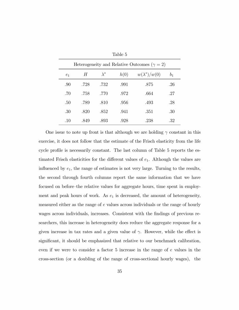
Table 5 shows the implied effects of differences in e1 from .1 to .9 for the case
of γ = 2.15
15Recall that a proportional shift in the e(λ) profile has no effect on hours of work in ourmodel, so that it is the ratio e1/e0 that matters and not e0 − e1.
34
Table 5
Heterogeneity and Relative Outcomes (γ = 2)
e1 H λ∗ h(0) w(λ∗)/w(0) b1
.90 .728 .732 .991 .875 .26
.70 .758 .770 .972 .664 .27
.50 .789 .810 .956 .493 .28
.30 .820 .852 .941 .351 .30
.10 .849 .893 .928 .238 .32
One issue to note up front is that although we are holding γ constant in this
exercise, it does not follow that the estimate of the Frisch elasticity from the life
cycle profile is necessarily constant. The last column of Table 5 reports the es-
timated Frisch elasticities for the different values of e1. Although the values are
influenced by e1, the range of estimates is not very large. Turning to the results,
the second through fourth columns report the same information that we have
focused on before—the relative values for aggregate hours, time spent in employ-
ment and peak hours of work. As e1 is decreased, the amount of heterogeneity,
measured either as the range of e values across individuals or the range of hourly
wages across individuals, increases. Consistent with the findings of previous re-
searchers, this increase in heterogeneity does reduce the aggregate response for a
given increase in tax rates and a given value of γ. However, while the effect is
significant, it should be emphasized that relative to our benchmark calibration,
even if we were to consider a factor 5 increase in the range of e values in the
cross-section (or a doubling of the range of cross-sectional hourly wages), the
35
aggregate consequences are still very large—a 20% increase in taxes still leads to a
decrease in hours of work of more than 15%.
It is important to note that the other studies that we referred to were based
on indivisible labor models, i.e., they assumed that hours of work conditional
upon employment were exogenous and equal for all workers. In our model, there
is a nonconvexity that leads to outcomes that are similar to what happens with
indivisible labor, but hours of work are endogenous and respond to changes in
the environment. This is significant, since a comparison of the results for relative
values of λ∗ and h(0) shows that as e1 decreases, the drop in λ∗ becomes smaller,
but the drop in h(0) actually increases. When e1 = .9, the drop in h(0) is basically
one percent, while when e1 = .1 the drop in h(0) exceeds seven percent. Precisely
because of this opposing effect on h(0), a comparison of the second and third
columns indicates that changes in e1 have a much larger effect on λ∗ than on
H. Two important messages follow from these results. First, an indivisible labor
model may preclude an important margin of adjustment in some contexts. Second,
the effect of taxes on hours of work for employed individuals is not purely a
function of the parameter γ—this table illustrates that the response in h(0) is
jointly determined with the response in λ∗.
There is one additional point of interest to note concerning heterogeneity. In
our model we assumed that there is no heterogeneity within a cohort. One may
conjecture that adding heterogeneity within a cohort will further diminish our
aggregate effects. However, at least one form of within cohort heterogeneity will
have no impact on our findings. Specifically, assume that within each cohort there
36
is a distribution of permanent productivities, represented as proportional shifts of
the productivity profile e(λ). As noted earlier, with u(c) = log(c), proportional
shifts of the productivity profile have no impact on the lifetime hours profile, and
so this form of heterogeneity would have no impact on our findings.
4.3. An Alternative Source of Life Cycle Variation
In the preceding analysis we assumed that the driving force for life cycle variation
in hours of work was exogenous variation in individual productivity over the life
cycle. Though this assumption underlies much of the literature on estimating labor
supply elasticities using micro data, there is probably good reason to question
the reasonableness of the assumption that productivity will double from young
to middle age independently of labor supply decisions over that period. Recent
work by Imai and Keane (2005) departs from this assumption by considering the
possibility that future wages are influenced by human capital that is accumulated
via a learning by doing process. While it is of interest to examine human capital
accumulation in the context of our model, we leave this possibility for future work.
But in this subsection we briefly describe the results that emerge from considering
a different driving force for life cycle variation in hours worked. Specifically, rather
than assuming that productivity varies with age we assume that the disutility of
work varies exogenously with age, so that preferences are now given by:
Z 1
0
[u(c(a))− e(a)v(h(a))]da (4.14)
37
where we assume that the profile e(a) is U -shaped. The mapping from time spent
at work to labor services is now given by:
l = g(h) (4.15)
where g is assumed to have the same shape as before.
Analogous to before, the optimal labor supply decision entails a reservation
disutility level, and hours worked when employed will be decreasing in the level
of disutility. Although there is no exogenous variation in productivity over the
life cycle, one can show that there will still be a positive relationship between
hours and wages per unit of time because of the properties of the g function. It
follows that this specification can still account for the standard life cycle patterns
in hours of work and wages. Moreover, at a qualitative level equilibrium in this
model is determined just as before—one can again represent the equilibrium as the
intersection of two curves in h(0)− λ∗ space.
When we carry out the numerical analysis analogous to that carried out above,
we get virtually identical results, and so in the interest of space we do not go into
them in any detail. Specifically, we find that the aggregate effect of the increase
in taxes is both large and virtually independent of the Frisch elasticity estimated
from life cycle data for prime aged individuals. One difference between the two
specifications is that it takes considerably greater variation in e(λ) in the variable
disutility case than it does in the variable productivity case, owing to the fact
that variable disutility affects wages over the life cycle only indirectly via the g(h)
function, while in the case of variable productivity there is also a direct effect. In
38
line with our earlier results about the role of increased heterogeneity, we find that
subject to matching a wage range of factor 2 over the life cycle, the aggregate
effects are slightly smaller than in the variable productivity case, yielding relative
hours of about .82 rather than .78. The point that we want to stress is simply
that the previous results are robust to this alternative driving force for life cycle
variation in hours worked.
5. Taxes and Market Work: Continental Europe and the
US
In this section we use the life cycle model developed earlier to discuss the ability
of tax and transfer policies to account for observed differences in hours worked
between the US and several countries in continental Europe.
5.1. Hours and Employment in Europe and the US
It is well known that hours of market work per person of working age are much
lower in continental Europe than in the US. In this section we present data to
establish two further properties. First, the large differences in total hours is the
result of important differences along two margins: the employment to population
ratio and annual hours worked per person in employment. Second, the differences
in employment to population ratios are due almost exclusively to differences in
this ratio for young and old workers. We deal with each of these in turn.
Cross-country data sets on hours of work allow one to decompose total an-
nual hours of work into two components: the number of people employed, and
39
the annual hours worked per person in employment. In making cross-country
comparisons it is necessary to normalize employment relative to some measure of
population. In what follows we use the size of the population aged 15-64, though
the empirical findings are not sensitive to this choice. Table 6 shows the relative
values for aggregate hours per person aged 15-64 (Hours/Pop), the employment
to working age population ratio (Emp/Pop), and annual hours of work per person
in employment (Hours/Emp) for four economies in continental Europe relative to
the US. These data are for the year 2003.
Table 6
Market Work in Europe Relative to the US
Belgium France Germany Italy
Hours/Pop .71 .68 .73 .69
Emp/Pop .83 .88 .91 .79
Hours/Emp .86 .77 .80 .87
The first row shows the well-known fact that market work in these economies is
only about 70% of the US level. The next two rows show that this large difference
in market work is the combination of large differences both along the employment
and the hours per employee margin. On average across the four economies, the
hours per person in employment margin accounts for slightly more than half of the
aggregate difference. While some of the differences both among these countries
and between these countries and the US is due to differences in the volume of part
time employment, this is not the dominant difference in differences in hours per
person in employment.
40
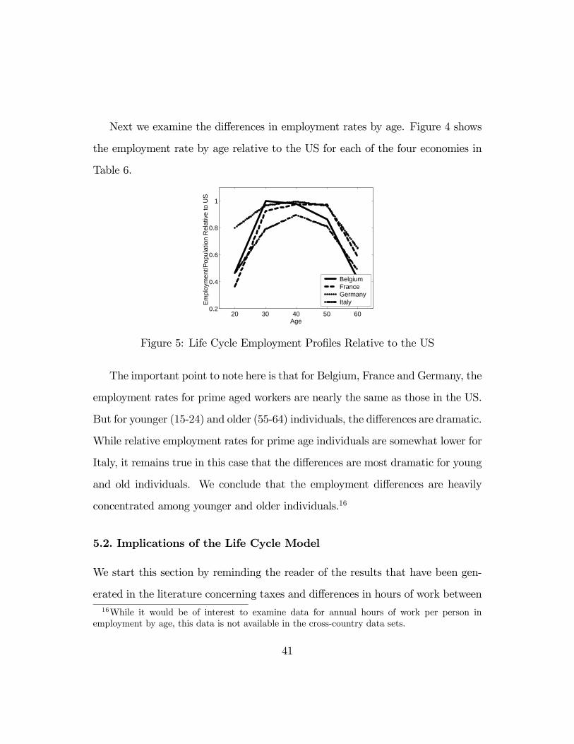
Next we examine the differences in employment rates by age. Figure 4 shows
the employment rate by age relative to the US for each of the four economies in
Table 6.
20 30 40 50 600.2
0.4
0.6
0.8
1
Age
Empl
oym
ent/P
opul
atio
n R
elat
ive
to U
S
BelgiumFranceGermanyItaly
Figure 5: Life Cycle Employment Profiles Relative to the US
The important point to note here is that for Belgium, France and Germany, the
employment rates for prime aged workers are nearly the same as those in the US.
But for younger (15-24) and older (55-64) individuals, the differences are dramatic.
While relative employment rates for prime age individuals are somewhat lower for
Italy, it remains true in this case that the differences are most dramatic for young
and old individuals. We conclude that the employment differences are heavily
concentrated among younger and older individuals.16
5.2. Implications of the Life Cycle Model
We start this section by reminding the reader of the results that have been gen-
erated in the literature concerning taxes and differences in hours of work between16While it would be of interest to examine data for annual hours of work per person in
employment by age, this data is not available in the cross-country data sets.
41
Europe and the US in the context of a standard (i.e., infinitely lived agent and di-
visible labor) model. As shown in Prescott (2004), differences in tax and transfer
policies of the type considered in the previous section can generate large differ-
ences in hours of work across economies. In particular, assuming that preferences
were log linear in consumption and leisure, Prescott shows that differences in tax
rates on the order of 20% can account for most of the differences in aggregate
hours worked between Europe and the US. Such a model necessarily abstracts
from the issue of how the hours differences are decomposed into differences in
employment rates and differences in hours per employee, and to what extent the
differences vary over the life cycle. Given that the data reveals some important
patterns across these other dimensions, it seems of interest to seek to understand
these differences in addition to those at the aggregate level. In principle, these
patterns may contain additional information that helps us evaluate the mechanism
at work in the standard model.
Based on the analysis in the previous section, it should be clear that our life
cycle model is able to generate not only large differences in aggregate hours in
response to differences in tax and transfer policies, but also that it qualitatively
matches the patterns found in the more disaggregated data as well. In particular,
we showed in the previous section that an increase in taxes will both lower the
hours profile and decrease the fraction of life spent in employment, implying that
there is a response along both margins. Moreover, given that the age profile for
λ is single peaked, this necessarily implies that the employment differences are
concentrated among young and old workers. It follows that at a qualitative level,
42
the extension of the analysis to a life cycle setting with a nonconvexity present in
the relationship between the provision of time and labor services is successful in
helping us understand the additional patterns in the data.
However, although the extension is successful at a qualitative level, the quan-
titative analysis in the previous section raises some concern about the ability of
the model to match both standard micro elasticity estimates as well as generate
changes on the employment and hours per employee margins that are consistent
with the cross-country differences. In particular, the cross-country differences sug-
gest that the employment and hours per employee margins are of roughly equal
importance. If we look at the results in Table 2, one sees that in response to higher
tax rates, our model will generate roughly equal responses in the two margins only
if the value of γ is relatively small, on the order of .5. Referring to Table 1, this
value of γ results in a Frisch elasticity based on life cycle data that exceeds 1.25.
Such a value is certainly large relative to estimates based on male labor supply.
The preceding discussion raises the issue that the model may have difficulty
in reconciling the relative variation in time devoted to market work along the two
margins. In the remainder of this section we propose a modification that can
qualitatively address this issue.
5.3. Retirement Policies
The tax and transfer policy that we analyzed in the previous section assumed
that workers receive a transfer at each instant of their life. It should be apparent,
however, that it is the present value of the transfer that matters, and not the
43
timing of the transfer. As a result, our previous analysis can also be used to assess
the consequences of a retirement program in which all workers are taxed at the
proportional rate τ while working, and then receive a constant transfer payment
from some age a onward, assuming that the retirement benefit is independent of
the labor supply decision. Our analysis can also be applied to the case in which
both types of transfers exist—one component that the individual receives at each
instant, and another component that is received as a retirement benefit. Since
retirement programs are one of the largest tax and transfer programs run by most
governments, it is important to know that our framework can be applied to this
type of program.
An important next step in the research program that analyzes the effects of tax
and transfer schemes on cross-country differences in market work is to perform a
thorough quantitative analysis of how various features of retirement contributions
and benefits influence lifetime labor supply decisions. Our goal here is much
more modest—we show how one particular feature of retirement programs may
be important for the relative division of hours differences along the employment
and hours per employee margin. The feature that we focus on is the fact that
many retirement programs contain a provision that imposes a minimum number
of years of full-time work in order to qualify for full benefits. Of course, if such
a provision is present, it does not follow that it will necessarily bind—this will
depend upon the costs and benefits to the individual of choosing a working life
that does not meet this requirement. In what follows here, we will simply ask
what the consequences of a binding constraint are and not deal with the issue of
44
under what circumstances the constraint might bind.
In order to understand how a tax and transfer program with a restriction on
required years of employment impacts on lifetime labor supply, it is instructive
to first consider the effect of a policy that simply stipulates the length of working
life in the absence of any taxes or transfers. To this end, consider a policy which
stipulates the length of working life to be λ. The next proposition describes how
this policy effects the hours profile.
Proposition 6: A change in λ that is binding leads to a shift in the opposite
direction for h(0), and hence the entire hours profile.
Proof: The impact of such a policy can be derived by setting λ∗ = λ and using
the first order condition for the h(λ) profile to determine the effect on hours. It
remains true that the entire h(λ) profile can be inferred from the value of h(0),
and that a higher value of h(0) implies a higher value for all other h(λ) as well.
To determine whether h(0) shifts up or down, we note that following expression
must hold:
1 = [
Z λ
0
e(λ)g(h(λ))dλ]v0(h(λ))
e(λ)g0(h(λ))(5.1)
Holding the h profile fixed, an increase in λ leads to an increase in the right hand
side. Since the right hand side is increasing in h(0) for a given λ it follows that
the hours profile must shift downward.//
This result is intuitive—if you force the individual to spend a greater fraction
of their life in employment than is optimal, they respond by decreasing the time
devoted to work while employed. A change in λ is effectively a move along the
volume of work curve in Figure 3. The significance of this result is that it shifts
45
work between the two components.
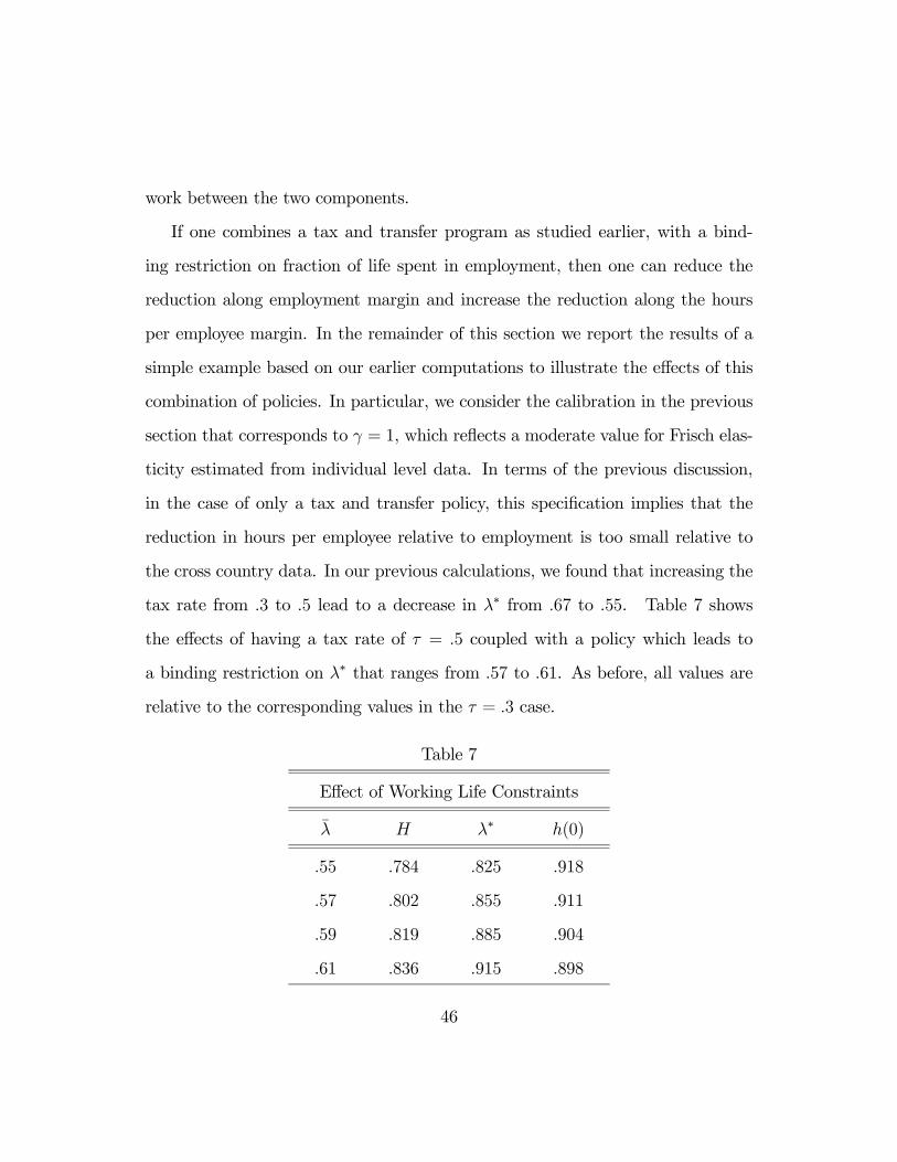
If one combines a tax and transfer program as studied earlier, with a bind-
ing restriction on fraction of life spent in employment, then one can reduce the
reduction along employment margin and increase the reduction along the hours
per employee margin. In the remainder of this section we report the results of a
simple example based on our earlier computations to illustrate the effects of this
combination of policies. In particular, we consider the calibration in the previous
section that corresponds to γ = 1, which reflects a moderate value for Frisch elas-
ticity estimated from individual level data. In terms of the previous discussion,
in the case of only a tax and transfer policy, this specification implies that the
reduction in hours per employee relative to employment is too small relative to
the cross country data. In our previous calculations, we found that increasing the
tax rate from .3 to .5 lead to a decrease in λ∗ from .67 to .55. Table 7 shows
the effects of having a tax rate of τ = .5 coupled with a policy which leads to
a binding restriction on λ∗ that ranges from .57 to .61. As before, all values are
relative to the corresponding values in the τ = .3 case.
Table 7
Effect of Working Life Constraints
λ H λ∗ h(0)
.55 .784 .825 .918
.57 .802 .855 .911
.59 .819 .885 .904
.61 .836 .915 .898
46
The first row in this table simply repeats the results from the case in which
there is no constraint on working life. As λ is increased from this value, we see
that the reduction in λ decreases, while the reduction in h(0) increases, as implied
by our analytic results. It is of interest to note that the reduction in H is also
reduced by the increase in λ, so that while this policy does serve to produce
changes in λ and h(0) that are more in line with cross country observations, one
of the consequences is to imply somewhat smaller responses at the aggregate level.
6. Conclusion
In this paper we develop a general equilibrium life cycle model of labor supply
that incorporates both intensive and extensive margins of labor supply. In the
equilibrium of our model, individuals have well-defined working lives, in the sense
that they enter the workforce at some point in their life and then work continuously
until some later point, at which time they withdraw from employment and do not
work again. We then use this model to analyze the implications for observed
differences in tax and transfer programs between the US and several countries
in continental Europe. In the context of this exercise we can use our model to
compute micro labor elasticities using life cycle variation in hours and wages for
prime age workers, as well as macro labor elasticities using variation in aggregate
hours across economies. Our analysis produces four main findings. First, macro
elasticities and micro elasticities are virtually unrelated: a factor 25 difference in
micro elasticities is associated with only a thirty percent change in the associated
macro elasticities. Second, macro elasticities are large—in the range of 2.3 − 3.0.
47
Third, in our model with variation in either productivity or disutility of work over
the life cycle, tax and transfer programs necessarily imply that higher taxes lead
to less work on both the extensive and intensive margin. Fourth, the employment
differences generated by differences in tax and transfer programs are necessarily
concentrated among young and old workers.
There are many natural extensions of interest. In terms of understanding life
cycle variation in wages and hours of work it is of interest to consider alternatives
which stress endogenous accumulation of human capital.17 In terms of assessing
the implications of tax and transfer programs for hours of work it is of interest to
consider a richer description of how tax and transfer programs interact with age
and productivity. Lastly, while our analysis has addressed the issue of reconciling
micro and macro elasticities in the context of permanent differences in tax and
transfer programs, there is a related issue of reconciling micro and macro elas-
ticities in the context of business cycle fluctuations which our analysis does not
specifically address.18
References
[1] Alesina, A., Glaeser E., and Sacerdote B., “Work and Leisure in the US and
Europe: Why So Different?,” NBER Macroeconomics Annual, 2005.17Two recent examples are Imai and Keane (2005) and Ljungqvist and Sargent (2007). The
latter also examines the implications for tax and transfer programs.18Chang and Kim (2006) pursue this issue in a model with incomplete markets, idiosyncratic
shocks and indivisible labor.
48
[2] Blundell R., and MaCurdy T., “Labor Supply: A Review of Alternative
Approaches,” in Handbook of Labor Economics Volume 3, pages 1559-1665,
edited by O. Ashenfelter and D. Card, North Holland, Amsterdam, 1999.
[3] Chang, Y., and Kim S., “Heterogeneity and Aggregation in the Labor Mar-
ket: Implications for Aggregate Preference Shifts,” mimeo, Seoul National
University, 2006b.
[4] Chang, Y., and Kim S., “From Individual to Aggregate Labor Supply: A
Quantitative Analysis Based on a Heterogeneous Agent Macroeconomy,” In-
ternational Economic Review 47(2006a), 1-27.
[5] Conesa, J., and Kehoe T., “Productivity, Taxes and Hours Worked in Spain,
1970-2003,”, mimeo, 2005.
[6] Davis, S., and Henreksson M., “Tax Effects on Work Activity, Industry Mix
and Shadow Economy Size: Evidence from Rich Country Comparisons”,
NBER Working Paper #10509, 2004.
[7] Heckman, J., “Life Cycle Consumption and Labor Supply: An Explanation
of the Relationship between Income and Consumption Over the Life Cycle,”
American Economic Review 64 (1974), 188-194.
[8] Heckman, J., “What Has Been Learned About Labor Supply in the Past
Twenty Years?,” American Economic Review 83 (1993), 116-121.
[9] Heckman J., and MaCurdy, T., “A Life Cycle Model of Female Labour Sup-
ply,” Review of Economic Studies 47 (1980), 47-74.
49
[10] Imai, S., and Keane M., “Intertemporal Labor Supply and Human Capital
Accumulation,” International Economic Review 45 (2004), 601-641.
[11] Ljungqvist, L., and Sargent, T., “Do Taxes Explain European Employ-
ment? Indivisible Labor, Human Capital, Lotteries and Savings”, forthcom-
ing, NBER Macroeconomics Annual.
[12] Lucas, R.E., and L. Rapping, “Intertemporal Substitution of Leisure in the
Theory of Labor Supply,” Journal of Political Economy 77 (1969), 721-754.
[13] MaCurdy, T., “An Empirical Model of Labor Supply in a Life Cycle Setting,”
Journal of Political Economy 89 (1981), 1059-1085.
[14] McDaniel, C. ,“Effective Tax Rates for 15 OECD Countries: 1950-2003,”
mimeo, 2006.
[15] Mendoza, E., Razin A., and Tesar L., “Effective Tax Rates in Macroeco-
nomics: Cross-Country Estimates of Tax Rates on Factor Incomes and Con-
sumption,” Journal of Monetary Economics 34 (1994), 297-323.
[16] Mincer, J., “Labor Force Participation of Married Women: A Study of Labor
Supply,” in H.G. LJ: Princeton University Press 1962, 63-97.
[17] Mulligan, C., “Aggregate Implications of Indivisible Labor,” Advances in