Page 1
Smart micro‐gridsProperties, trends and local control of energy sources
UNICAMP – UNESP, August 2012
Green Technologies enabling Energy Saving
1
Paolo Tenti, Alessandro Costabeber
Department of Information Engineeering
University of Padova
Page 2
Outline1. From the traditional grid to the smart grid
2. The potential revolution of the smart micro-grid
3. Smart micro-grid architecture
4. The role of energy storage
5. Control issues in smart micro-grids
6. Inverter modeling and control
Smart micro‐gridsProperties, trends and local control of energy sources
2
6. Inverter modeling and control
7. Micro-grid modeling and distribution loss analysis
8. Optimum control of smart micro-grids
9. On-line Identification of micro-grid parameters
10. Distributed surround control of smart micro-grids
11. Distributed cooperative control of smart micro-grids
12. Simulation results
13. Conclusions
Page 3
Smart micro‐gridsProperties, trends and local control of energy sources
UNICAMP – UNESP, August 2012
Green Technologies enabling Energy Saving
3
1. From the traditional grid to the smart grid
Page 4
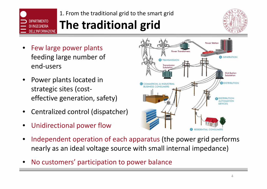
• Few large power plants
feeding large number of
end-users
• Power plants located in
strategic sites (cost-
effective generation, safety)
1. From the traditional grid to the smart grid
The traditional grid
effective generation, safety)
• Centralized control (dispatcher)
• Unidirectional power flow
• Independent operation of each apparatus (the power grid performs
nearly as an ideal voltage source with small internal impedance)
• No customers’ participation to power balance
4
Page 5
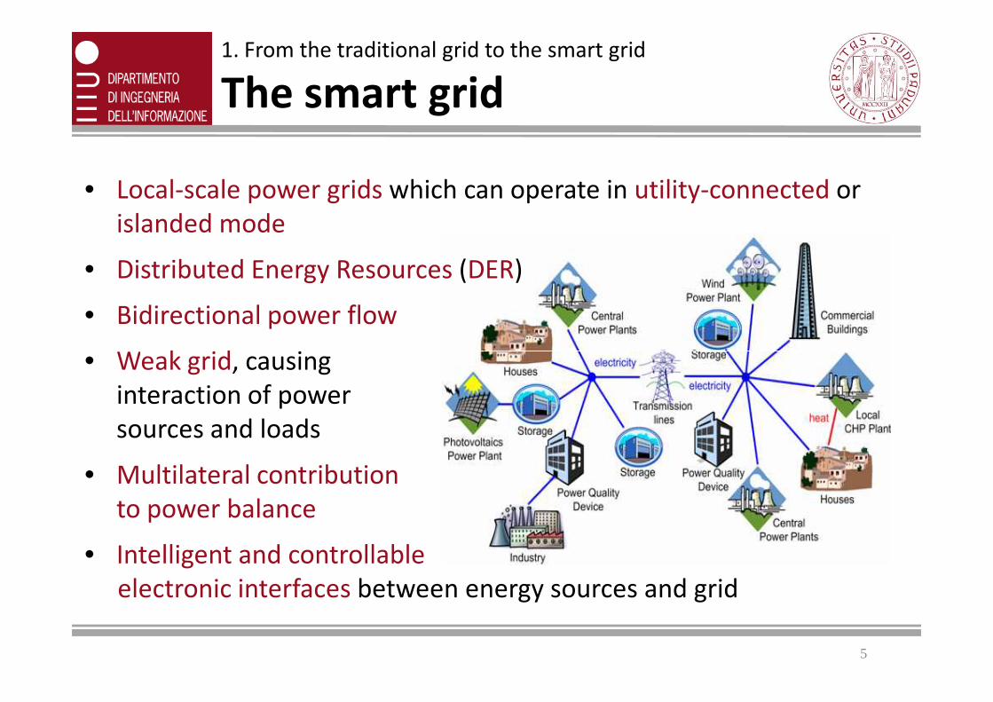
• Local-scale power grids which can operate in utility-connected or
islanded mode
• Distributed Energy Resources (DER)
• Bidirectional power flow
• Weak grid, causing
1. From the traditional grid to the smart grid
The smart grid
• Weak grid, causing
interaction of power
sources and loads
• Multilateral contribution
to power balance
• Intelligent and controllable
electronic interfaces between energy sources and grid
5
Page 6
• Distributed renewable resources
• less carbon footprint • energy cost reduction
• Energy efficiency• power sources close to loads• improved demand response
1. From the traditional grid to the smart grid
Benefits of the smart grid
• improved demand response
• Improved utilization of conventional power sources• less active, reactive, unbalance and distortion power
flowing through the distribution lines
• Voltage support• distributed injection of active and reactive power
• Increased hosting capacity• without investments in the grid infrastructure
6
Page 7
• Bidirectional power flow• need for new control and protection strategies
• conventional voltage stabilization techniques not applicable
• Weak grid (non-negligible internal impedance, especially in
islanded operation)
1. From the traditional grid to the smart grid
Challenges of the smart grid
islanded operation)
• voltage distortion due to nonlinear loads
• voltage asymmetry due to unbalanced loads and single-phase DER units (PV, batteries, …)
• Irregular power injection by renewable energy sources
• need for power flow regularization and peak power shaving
• need for energy storage devices
7
Page 8
Smart micro‐gridsProperties, trends and local control of energy sources
UNICAMP – UNESP, August 2012
Green Technologies enabling Energy Saving
8
2. The potential revolution of the smart micro‐grid
Page 9
MV/LV Substation
Residential 1ϕLOAD
Residential 1ϕLOAD + PV DG +
ES
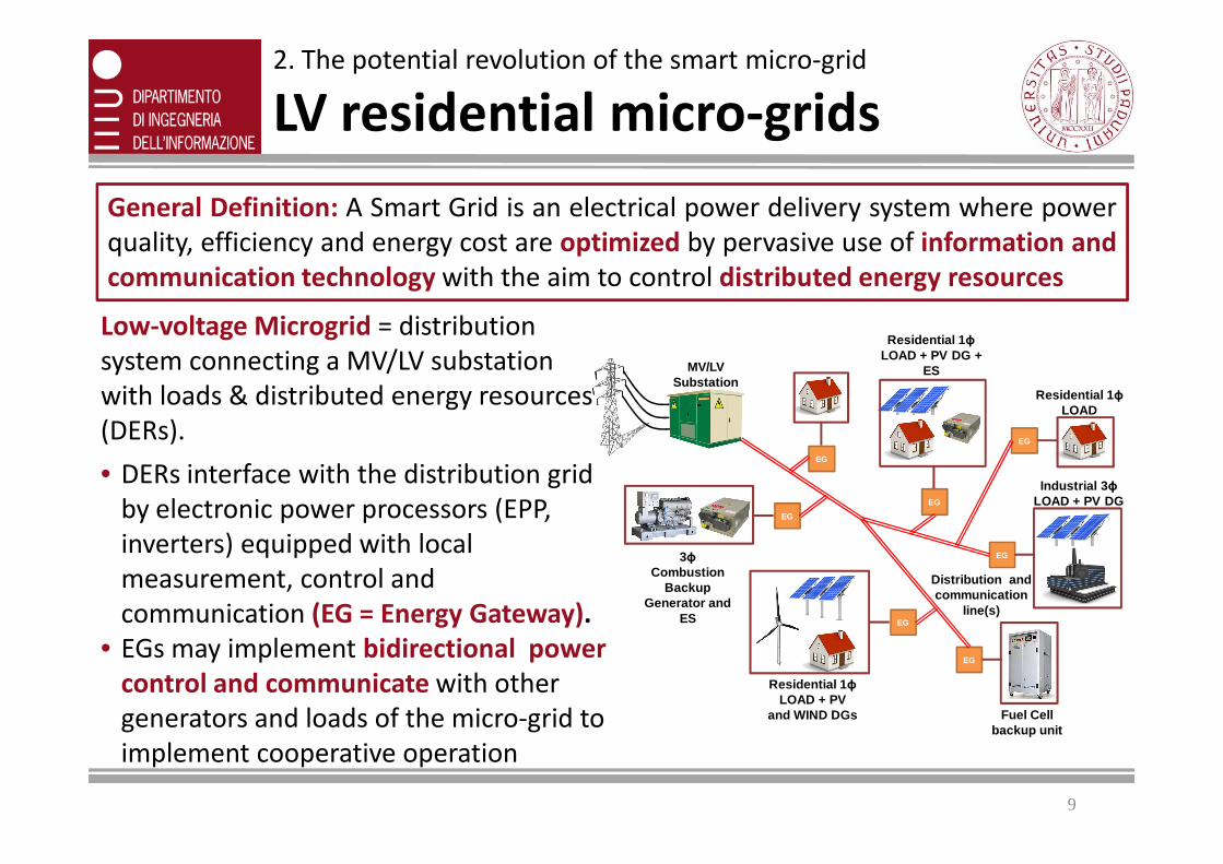
General Definition: A Smart Grid is an electrical power delivery system where power
quality, efficiency and energy cost are optimized by pervasive use of information and
communication technology with the aim to control distributed energy resources
Low‐voltage Microgrid = distribution
system connecting a MV/LV substation
with loads & distributed energy resources
(DERs).
2. The potential revolution of the smart micro-grid
LV residential micro‐grids
EG
EG
EG
EG
EG
EG
EG
Residential 1ϕLOAD + PV
and WIND DGs
3ϕCombustion
Backup Generator and
ES
Fuel Cellbackup unit
Industrial 3ϕLOAD + PV DG
Distribution and communication
line(s)
9
(DERs).
• DERs interface with the distribution grid
by electronic power processors (EPP,
inverters) equipped with local
measurement, control and
communication (EG = Energy Gateway).
• EGs may implement bidirectional power
control and communicate with other
generators and loads of the micro-grid to
implement cooperative operation
Page 10
Environment & savings
• Green power
• Full utilization of distributed
energy resources
• Reduced distribution loss
• Increased hosting capacity
• Increased power quality
2. The potential revolution of the smart micro-grid
Expected benefits of micro‐grids
• Increased power quality
even in remote locations
• Layered grid architecture
Social & economics
• Strengthen consumers role
• Develop communities of prosumers
• New functions and players in the energy market
• New arena for entrepreneurs, manufacturers and service providers
• New jobs for green collars
Paradigm: The INTERNET of ENERGY 10
Page 11
• Exploit every available energy source
• Minimize distribution losses and non-
renewable energy consumption
• Increase power quality and hosting
capacity
• Implement cheap ICT architectures for
distributed control and communication
2. The potential revolution of the smart micro-grid
Technological challenges
distributed control and communication
• Integrate micro-grid control and
domotics
• Revise accounting principles and
methodologies
• Restructure network protection
• Assure data security and privacy
• Pursue flexibility and scalability (from
buildings to townships)
11
Page 12
UE Roadmap for microUE Roadmap for micro--gridsgrids (CIGRE 2010)(CIGRE 2010)
2. The potential revolution of the smart micro-grid
The future of micro‐grids
Smart grid investment forecastSmart grid investment forecast (JRC report 2011)(JRC report 2011)
12
Page 13
Smart micro‐gridsProperties, trends and local control of energy sources
UNICAMP – UNESP, August 2012
Green Technologies enabling Energy Saving
13
3. Smart micro‐grid architecture
Page 14
local power &
EEnergynergy
GGatewayateway
EEnergynergy
GGatewayateway
EEnergynergy
GGatewayateway
UtilityUtility
IInterfacenterface
UtilityUtility
3. Micro-grid architecture
General sketch of a micro‐grid
energyenergy
storagestorage
energyenergy
storagestorage
local power &
communications gridGGatewayateway
EEnergynergy
GGatewayateway
EEnergynergy
GGatewayateway EEnergynergy
GGatewayateway
EEnergynergy
GGatewayateway
14
Page 15
3. Micro-grid architecture
Definitions and requirements
• Active grid nodes correspond to prosumers, i.e., buildings or residential
settlements equipped with distributed energy resources (DERs) and
Energy Gateways (EGs)
– DERs may be PV panels, wind turbines, fuel cells, batteries, flywheels, etc.
– EGs include an electronic power processor (EPP), capable to control the
active and reactive power flow from local sources into the grid, a local
control unit (LCU) and a smart meter (SM), which provides measurement,
15
control unit (LCU) and a smart meter (SM), which provides measurement,
communication and synchronization capability.
• Passive grid nodes correspond to traditional consumers and are assumed
to be equipped with smart meters too
• Plug & play operation of EGs ensures flexibility and scalability of the
micro-grid architecture
• Distributed control and communication allows cooperative operation of
EGs and synergistic utilization of DERs
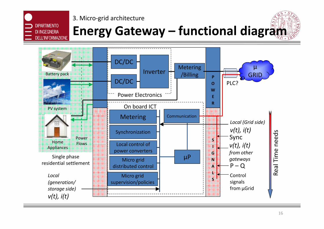
Page 16
On board ICT
Metering Communication
DC/DC
DC/DC
Inverter
Power Electronics
PV system
Battery packP
O
W
E
R
Metering
/Billing
PLC?
μ
GRID
3. Micro-grid architecture
Energy Gateway – functional diagram
Metering Communication
μP
Re
al
Tim
e n
ee
ds
Single phase
residential settlement
Power
FlowsHome
AppliancesLocal control of
power converters
Synchronization
Micro grid
distributed control
S
I
G
N
A
L
SMicro grid
supervision/policies
Sync
P – Q
Local (Grid side)
v(t), i(t)
v(t), i(t) from other
gateways
Control
signals
from μGrid
Local
(generation/
storage side)
v(t), i(t)
16
Page 17
Concept idea: micro-grid
to appear as an ‘ideal’
programmable load
Energy Storage
Power
Electronics
•Aggregator, enabling distributed EGs to
μ GRID
3. Micro-grid architecture
Utility Interface – functional diagram
Communication
with μ-Grid and
utility
I/O INTERFACE
•Aggregator, enabling distributed EGs to
contribute to system-level energy
management
•Energy backup in case of islanded
operation or grid dynamics
•Micro-grid interface to the utility,
managing system-level load balancing,
harmonic and reactive compensation,
aggregate demand response, etc.
Three phase
distribution
infrastructure
energy
gateways
17
Page 18
Gri
d
Use
r CONTROL
Communication
Interface
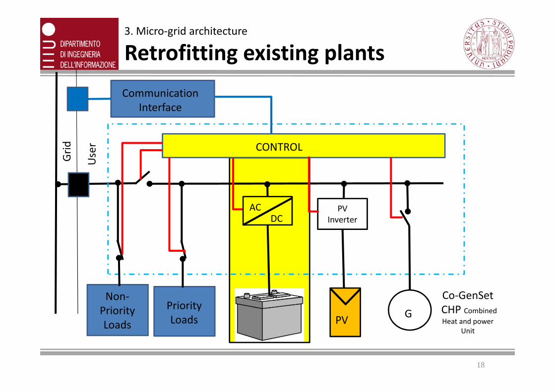
3. Micro-grid architecture
Retrofitting existing plants
Co-GenSet
CHP Combined
Heat and power
Unit
Non-
Priority
Loads
ACDC
PV
Inverter
PVG
Priority
Loads
18
Page 19
Smart micro‐gridsProperties, trends and local control of energy sources
UNICAMP – UNESP, August 2012
Green Technologies enabling Energy Saving
19
4. The role of energy storage
Skip
Page 20
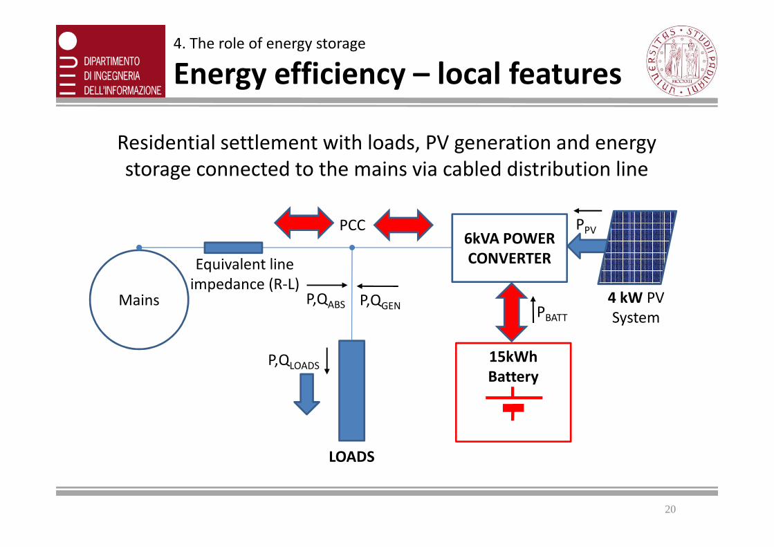
Residential settlement with loads, PV generation and energy
storage connected to the mains via cabled distribution line
PCC
Equivalent line
impedance (R-L)
6kVA POWER
CONVERTER
PPV
4. The role of energy storage
Energy efficiency – local features
PBATT
Mains
Equivalent line
impedance (R-L)4 kW PV
System
15kWh
BatteryP,QLOADS
LOADS
P,QGENP,QABS
20
Page 21
4
4.5
5Loads and PV generation
Pload
PPV
PCC
4kW PV
System
6kVA POWER
CONVERTER
15kWh
Battery
PPV
PBATT
P,QGEN
P,QLOADS
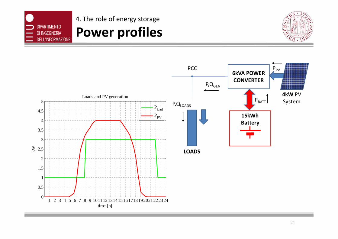
4. The role of energy storage
Power profiles
1 2 3 4 5 6 7 8 9 1011121314151617181920212223240
0.5
1
1.5
2
2.5
3
3.5
4
time [h]
kW
PV
Battery
LOADS
21
Page 22
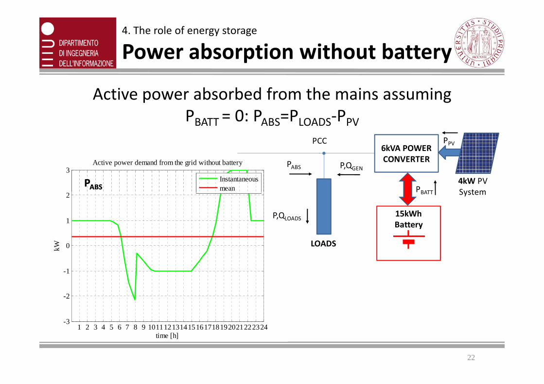
Active power absorbed from the mains assuming
PBATT = 0: PABS=PLOADS-PPV
2
3Active power demand from the grid without battery
Instantaneousmean
PCC
4kW PV
System
6kVA POWER
CONVERTER
PPV
PBATT
P,QGENPABS
PPABSABS
4. The role of energy storage
Power absorption without battery
1 2 3 4 5 6 7 8 9 101112131415161718192021222324-3
-2
-1
0
1
2
time [h]
kW
meanSystem
15kWh
Battery
PBATT
P,QLOADS
LOADS
22
Page 23
4. The role of energy storage
Distribution loss without battery
80
100
120
140Distribution loss without battery
Instantaneousmean
1 2 3 4 5 6 7 8 9 1011121314151617181920212223240
20
40
60
80
time [h]
W
23
Page 24
0.6
0.8
1Active power demand from the grid with battery
Instantaneousmean
PPABSABS=P=PLOADSLOADS‐‐PPPVPV‐‐PPBATTBATT
PCC
4kW PV
System
6kVA POWER
CONVERTER
PPV
PBATT
P,QGENPABS
Local control tends to enforce PLocal control tends to enforce PABSABS= P= PABS_AVGABS_AVG (daily average power)(daily average power)
4. The role of energy storage
Power absorption with battery
1 2 3 4 5 6 7 8 9 101112131415161718192021222324-1
-0.8
-0.6
-0.4
-0.2
0
0.2
0.4
0.6
time [h]
kW
System
15kWh
Battery
PBATT
P,QLOADS
LOADSDischargeDischarge
completecompleteChargeCharge
completecomplete
24
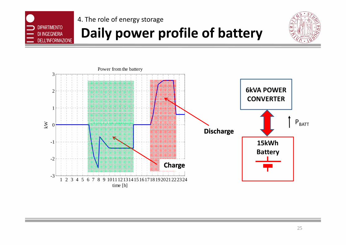
Page 25
0
1
2
3Power from the battery
kW
6kVA POWER
CONVERTER
PBATT
4. The role of energy storage
Daily power profile of battery
DischargeDischarge
1 2 3 4 5 6 7 8 9 101112131415161718192021222324-3
-2
-1
0
time [h]
kW
15kWh
Battery
PBATT
ChargeCharge
25
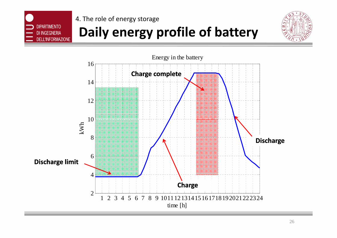
Page 26
10
12
14
16Energy in the battery
Charge completeCharge complete
4. The role of energy storage
Daily energy profile of battery
1 2 3 4 5 6 7 8 9 1011121314151617181920212223242
4
6
8
10
time [h]
kWh
ChargeCharge
DischargeDischarge
Discharge limitDischarge limit
26
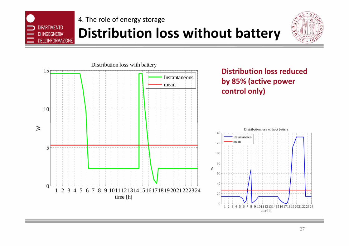
Page 27
Distribution loss reduced
by 85% (active power
control only)
4. The role of energy storage
Distribution loss without battery
10
15Distribution loss with battery
Instantaneousmean
1 2 3 4 5 6 7 8 9 1011121314151617181920212223240
5
time [h]
W
1 2 3 4 5 6 7 8 9 1011121314151617181920212223240
20
40
60
80
100
120
140Distribution loss without battery
time [h]W
Instantaneousmean
27
Page 28
Local functions (Energy Gateways)
• Regularization of power absorption
• Reduction of losses in the distribution feeder
• Peak power shaving
• Emergency supply in case of mains outage (UPS operation)
• Node voltage stabilization
4. The role of energy storage
Distributed energy storage
28
• Node voltage stabilization
• Prosumer energy bill reduction
Micro‐grid functions (Utility Interface + Energy Gateways)
• Energy sharing & backup in case of islanded operation
• Smoothing of irregular power generation by renewable sources
• Programmable active and reactive power absorption
• Power delivery to the utility on demand
• Cost‐effective energy management and ROI planning
Page 29
Smart micro‐gridsProperties, trends and local control of energy sources
UNICAMP – UNESP, August 2012
Green Technologies enabling Energy Saving
29
5. Control issues in smart micro‐grids
Page 30
Local control functions (Energy Gateways)
• Exploitation of renewable energy sources (active power control)
• Management of energy storage (active power control)
• Voltage support (active & reactive power control)
• Reactive & harmonic compensation
• Load shedding & shifting
5. Control issues in smart micro-grids
Control objectives
30
• Load shedding & shifting
Micro‐grid control functions (Utility Interface + Energy Gateways)
• Synergistic utilization of micro-grid resources
• Aggregate demand response and peak power shaving
• Load balancing by reactive current control (Steinmetz approach)
• Management of mains outages & grid dynamics
• Management of islanded operation
• Management of active and reactive power requests by the utility
Page 31
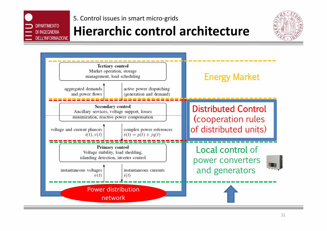
Distributed Control Distributed Control Distributed Control Distributed Control ((((cooperation rules
Energy MarketEnergy MarketEnergy MarketEnergy Market
5. Control issues in smart micro-grids
Hierarchic control architecture
31
Power distribution
network
Local control Local control Local control Local control of power converters and generators
((((cooperation rules of distributed units)
Page 32
Smart micro‐gridsProperties, trends and local control of energy sources
UNICAMP – UNESP, August 2012
Green Technologies enabling Energy Saving
32
6. Inverter modeling and control
Page 33
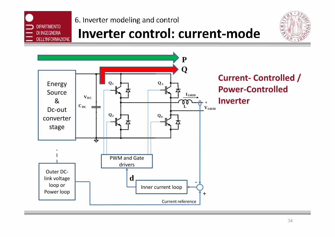
6. Inverter modeling and control
Inverter control modes
Single-phase voltage-fed full-bridge grid-connected inverters can be driven
according to different control approaches:
1. Current‐mode control: the ac-side inductor current is controlled to track a
current reference set by the DC link voltage controller (typical configuration
33
current reference set by the DC link voltage controller (typical configuration
of PV systems) or by an external power loop. The inverter appears as a
Controlled current (or Power) source.
2. Voltage‐mode control: the current loop is driven by an external voltage
control loop that tracks a voltage reference (UPS applications or droop-
controlled inverters, where the power flows are controlled by acting on
module and phase of the inverter ac voltage). The inverter appears as a
Controlled voltage source.
Page 34
C DC
Q1
VDC
Q2
Q 3
Q4
+ VGRID
I GRID
L
Energy
Source
&
Dc-out
converter
PQ
Current‐ Controlled /
Power‐Controlled
Inverter
converter
stage
PWM and Gate
drivers
dInner current loop
-
+Current reference
Outer DC-
link voltage
loop or
Power loop
34
Page 35
Voltage‐Controlled
Inverter
CDC
Q1
VDC
Q
Q3
Q
+ VGRID IGRID
L C
Energy
Source
&
Dc-out
converter
PQ
- + Output Voltage
reference
(from droop
35
Q2 Q4 converter
stage
PWM and Gate
drivers
dInner current loop
+
Current
reference
Gri
d V
olt
ag
e L
oo
p
(from droop
control, P-Q
control, minimum-
loss control etc.)
Page 36
For current-controlled inverters the usual requirement in grid-connected
operation (e.g., for PV inverters) is to supply purely active power, i.e., to inject a
current in phase with the line voltage (cosϕ=1);
Assuming sinusoidal grid voltage VGRID and inverter current IGRID, the phasorial
representation of this operating condition is:
V&I& GRIDV&GRIDI&
In general, however, the inverter can feed a current which
can be leading or lagging the grid voltage
GRIDV&
GRIDI&
ϕ−i
v
jGRIDGRID
jGRIDGRID
eII
eVVϕ
ϕ
=
=&
&
RMS values
iv ϕϕϕ −=
36
Page 37
Complex Power supplied
by the inverter:
jQPIVS GRIDGRID +== *&&&
( ) == ϕ−eIVS*j
GRIDGRID&
Q
P>0: active power
injected into the grid
P<0: active power
absorbed from the
grid
Q>0: inductive
power injected into
Q>0:inductive power
injected into the grid
Four quadrant operation
37
( )
ϕ=ϕ=
ϕ+ϕ===
==ϕ
sinIVQ
cosIVP
sinIVcosIV
eIV
eIVS
GRIDGRID
GRIDGRID
GRIDGRIDGRIDGRID
jGRIDGRID
GRIDGRID&
P
P>0: active power
injected into the
grid
P<0: active power
absorbed from the
grid
power injected into
the grid (lagging
current, φ<0)
Q<0: capacitive
power injected into
the grid (leading
current, φ>0)
injected into the grid
(lagging current, φ<0)
Q<0 -> capacitive
power injected into
the grid (leading
current, φ>0)
Page 38
P
Q
P>0
Q>0
P>0
Q<0
P<0
Q>0
P<0
Q<0
In distributed generation, the inverters
operate in the I and IV quadrants,
injecting positive active power and
either positive or negative reactive
power
Inverter
Operation
Area
POWER RATING:
The complex power that can be
injected by an inverter is limited by
the current and voltage rating of the
components (V and I limits for the
switches, I limits for the output
inductors, V limit for the capacitors
etc)
For a given grid voltage, these limits
are represented by the apparent
power
]VA[SIVA maxmaxGRIDGRID&==
38
Page 39
Smart micro‐gridsProperties, trends and local control of energy sources
UNICAMP – UNESP, August 2012
Green Technologies enabling Energy Saving
39
7. Micro‐grid modeling and distribution loss analysis
Skip
Page 40
7. Micro-grid modeling and distribution loss analysis
Micro‐grid modeling (1)
To analyze the micro-grid operation, a suitable modelling is required.
Power Systems approach: Network elements are represented as constant power loads /
distributed generators, constant current loads, constant impedance loads. The grid is
analyzed in terms of Power Flow relations, resulting in nonlinear equation systems which
require numeric solvers (Newton-Raphson , etc).
LV distribution systems: the voltage is impressed at the Point of Common Coupling with
the mains and its variation along the LV grid is within ±5% of rated value. Thus, under
steady-state conditions, the constant-power loads can be represented as constant-current
PCCV&
eqZ&
GV&
GI&
40
steady-state conditions, the constant-power loads can be represented as constant-current
(or constant-impedance) elements. Similarly for the energy sources. Thus, the system
model becomes linear and can be solved analytically by Kirchhoff’s and load equations.
PCC=Point ofCommon Coupling (MV/LV sub.)
Moreover, LV distribution lines are usually
made by cables with constant section, i.e.
impedances with constant phase (modelled as
R-L series). This further simplifies the analysis,
making possible the analytical solution of
radial and meshed grids as well.
Page 41
Assumption: the PCC voltage is taken as phase reference for the phasorial representation
VjjUV ratedPCC 02300 +=+=&
Approximation: based on the assumption of
negligible phase voltage differences between
grid nodes, the active and reactive currents
absorbed by the loads or injected by the
generators nearly coincide with the real and
7. Micro-grid modeling and distribution loss analysis
Micro‐grid modeling (2)
41
generators nearly coincide with the real and
imaginary components of such node
currents referred to the PCC voltage.
PCCVV <<∆
PCCV&
eqZ&
GV&
GI&
• The real part of the node currents controls the
active power absorbed/injected at the grid
nodes
• The imaginary part of the node currents
controls the reactive power absorbed/injected
at the grid nodes
Page 42
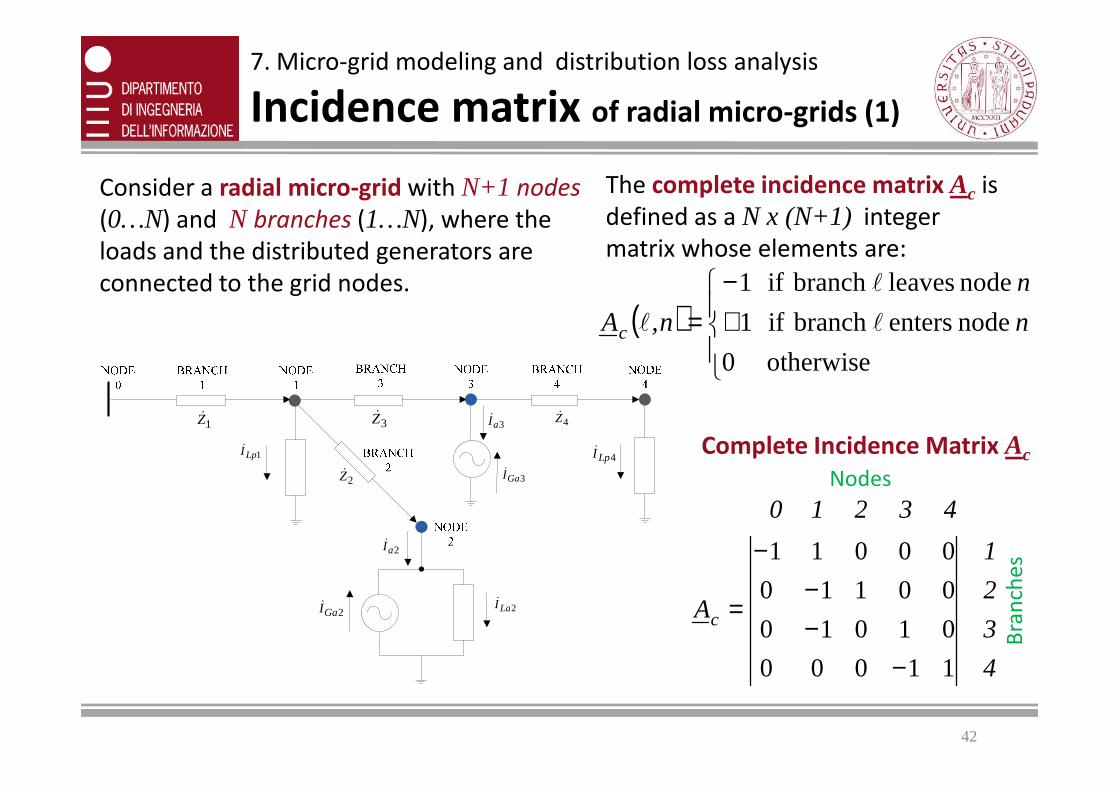
7. Micro-grid modeling and distribution loss analysis
Incidence matrix of radial micro‐grids (1)
Consider a radial micro‐grid with N+1 nodes
(0…N) and N branches (1…N), where the
loads and the distributed generators are
connected to the grid nodes.
( )
otherwise 0
node enters branch if 1
node leaves branch if 1
+−
= n
n
n,Ac l
l
l
The complete incidence matrix Ac is
defined as a N x (N+1) integer
matrix whose elements are:
42
Complete Incidence Matrix Ac
4
3
2
1
A
43210
c
11000
01010
00110
00011
−−−
−
=
Bra
nch
es
Nodes
1LpI&
2LaI&2GaI&
3GaI&
3aI&
2aI&
4LpI&
1Z&
2Z&
3Z& 4Z&
Page 43
7. Micro-grid modeling and distribution loss analysis
Incidence matrix of radial micro‐grids (2)
Reduced Incidence Matrix A
The reduced incidence matrix A is
defined as a N x N integer matrix
obtained by eliminating the column
of node 0 (slack node, i.e., the Point
of Common Coupling with the
utility, PCC)
43
Reduced Incidence Matrix A
4
3
2
1
A
4321
c
1100
0101
0011
0001
−−−
=
Bra
nch
es
Nodes
Note: The reduced Incidence
Matrix A is square and invertible
1LpI&
2LaI&2GaI&
3GaI&
3aI&
2aI&
4LpI&
1Z&
2Z&
3Z& 4Z&
Page 44
7. Micro-grid modeling and distribution loss analysis
Path matrix of radial micro‐grids
The transpose inverse of reduced
incidence matrix A is a N x Ninteger matrix called path matrix P ,
whose nth column gives the path
from node 0 to node n.
44
Path Matrix P
Bra
nch
es
Nodes
( ) ( )4
3
2
1
AAP
4321
TT
1000
1100
0010
1111
11 ===−−
1LpI&
2LaI&2GaI&
3GaI&
3aI&
2aI&
4LpI&
1Z&
2Z&
3Z& 4Z&
Page 45
7. Micro-grid modeling and distribution loss analysis
Kirchhoff’s laws of radial micro‐grids (1)
Let uc be the node voltages (including node
0) and v the branch voltages, the Kirchoff’s
Law for voltages (KLV) applied to voltage
phasors gives:
4
3
2
1
0
4
3
2
1
1100
0101
0011
0001
0
0
0
1
0
U
U
U
UU
V
V
V
V
uAv
Aa
cc
&
&
&
&
&
44 344 21
&
&
&
&
×
−−−
−
−=⇒−=
45
1LpI&
2LaI&2GaI&
3GaI&
3aI&
2aI&
4LpI&
1Z&
2Z&
3Z& 4Z&
0 Aa
In a simplified form, let u be
the node voltages (excluding
node 0), the Kirchoff’s Law for
voltages (KLV) becomes:
UAUaV &&& ×−⋅−= 00
where a0 is the first column of
complete incidence matrix Ac
Page 46
7. Micro-grid modeling and distribution loss analysis
Kirchhoff’s laws of radial micro‐grids (2)
Let ic be the node currents (including node 0,
with positive polarity if leaving the grid) and j
be the branch currents, the Kirchoff’s Law
for currents (KLC) applied to current phasors
gives:
4
3
2
1
4
3
2
1
0
1000
1100
0010
0111
0001
J
J
J
J
I
I
I
I
I
jAi Tcc
&
&
&
&
&
&
&
&
&
×−
−−−
=⇒=
46
1LpI&
2LaI&2GaI&
3GaI&
3aI&
2aI&
4LpI&
1Z&
2Z&
3Z& 4Z&
44 1000I&
In a simplified form, let i be
the node currents (excluding
node 0), the Kirchoff’s Law for
currents (KLC) becomes:
×=
×=
JAI
JaIT
T
&&
&&
00
Page 47
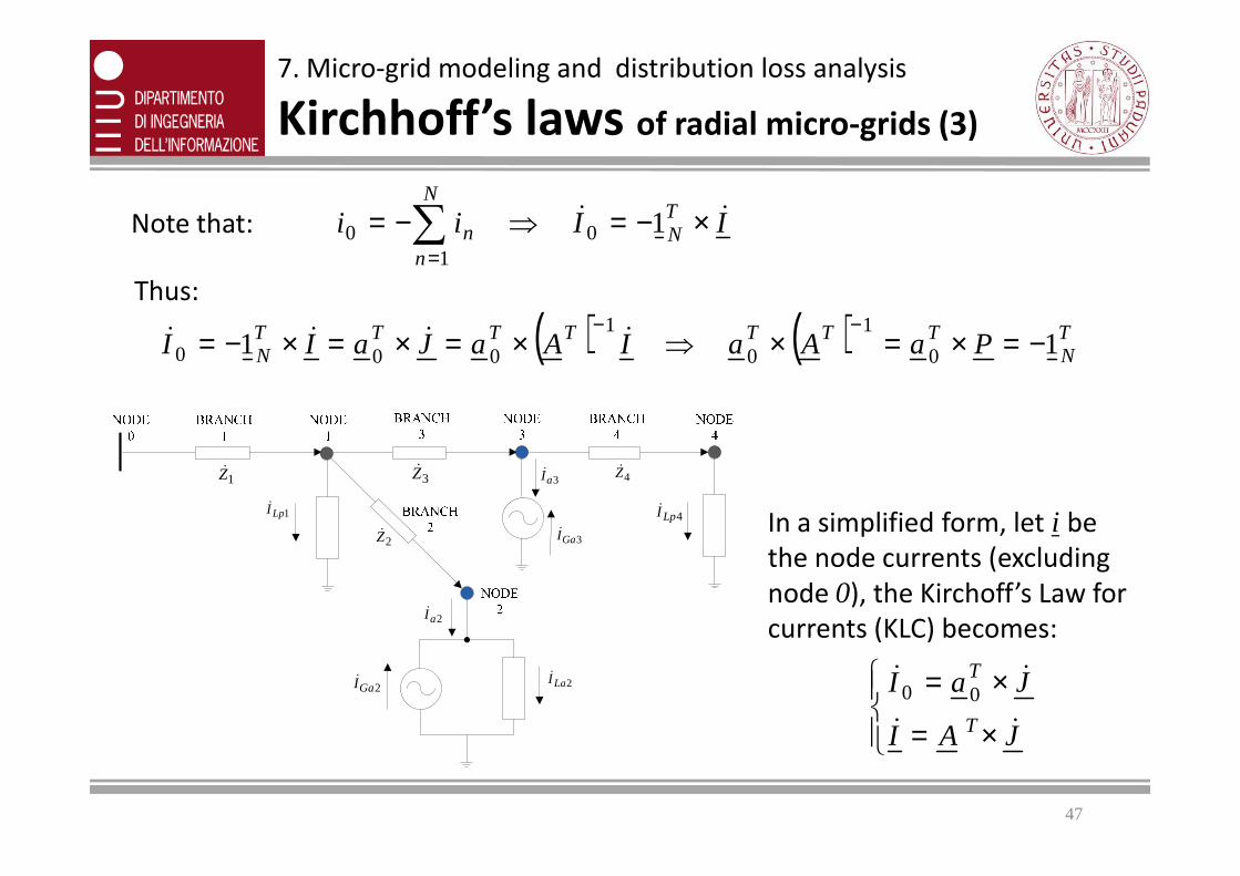
7. Micro-grid modeling and distribution loss analysis
Kirchhoff’s laws of radial micro‐grids (3)
Note that: ∑=
×−=⇒−=N
n
TNn IIii
100 1 &&
Thus:
( ) ( ) TN
TTTTTTTN PaAaIAaJaII 11 0
1
0
1
000 −=×=×⇒×=×=×−=−−
&&&&
47
1LpI&
2LaI&2GaI&
3GaI&
3aI&
2aI&
4LpI&
1Z&
2Z&
3Z& 4Z&
In a simplified form, let i be
the node currents (excluding
node 0), the Kirchoff’s Law for
currents (KLC) becomes:
×=
×=
JAI
JaIT
T
&&
&&
00
Page 48
7. Micro-grid modeling and distribution loss analysis
Radial micro‐grid equations (1)
1LpI&
2LaI&2GaI&
3GaI&
3aI&
2aI&
4LpI&
1Z&
2Z&
3Z& 4Z&
Branch impedances
Z1 1+j1 Ω
Z2 2+j2 Ω
Z3 3+j3 Ω
Z4 4+j4 Ω
Load currents
ILp1 5+j5 A
ILa2 10+j10 A
I 15+j15 A
48
For each branch of the distribution grid we can write: jiijjiij JZUUV →=−= &&&&&
ILp4 15+j15 A
JZV
Z
Z
Z
ZdiagZ
N
N ×=⇒== =&&
&
K
&
&
&&
ll
000
000
000
000
2
1
1
Let Z be the diagonal matrix of the branch impedances, in vector form we get:
Page 49
7. Micro-grid modeling and distribution loss analysis
Radial micro‐grid equations (2)
1LpI&
2LaI&2GaI&
3GaI&
3aI&
2aI&
4LpI&
1Z&
2Z&
3Z& 4Z&
Branch impedances
Z1 1+j1 Ω
Z2 2+j2 Ω
Z3 3+j3 Ω
Z4 4+j4 Ω
Load currents
ILp1 5+j5 A
ILa2 10+j10 A
I 15+j15 A
49
Recalling the previous definitions and results we get:
ILp4 15+j15 A
( ) IAZUAUaJAI
UAUaVJZV
P
TT
&
321
&&&
&&
&&&
&& ××−=×+⇒
×=×−−=
⇒×=−1
0000
IZUIPZPUUIPZAUUaA grid
Z
T
U
N
P gridT
N
&&&&
43421
&
321
&&&&&&
43421
&&
×−=×××−=⇒×××−=+× −
−
−00
10
1
01
0
1
The grid equations can therefore be expressed as a function of node currents and
voltages in the form:
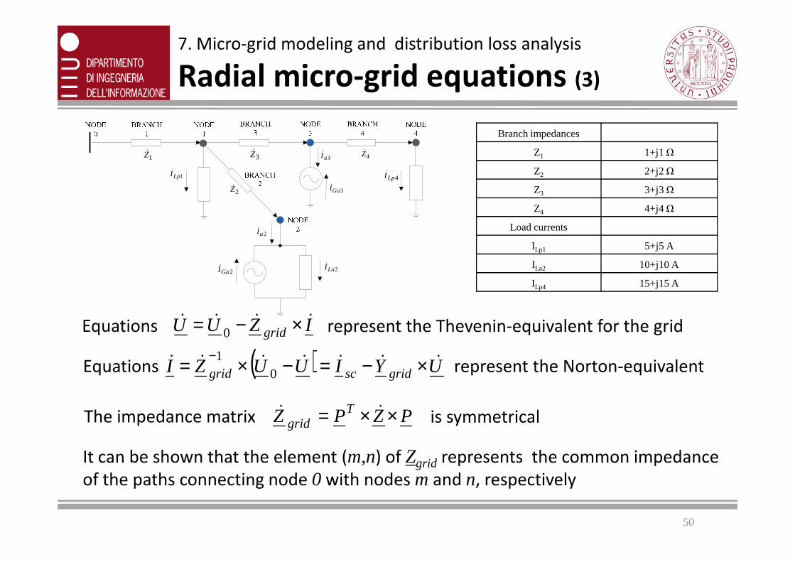
Page 50
7. Micro-grid modeling and distribution loss analysis
Radial micro‐grid equations (3)
1LpI&
2LaI&2GaI&
3GaI&
3aI&
2aI&
4LpI&
1Z&
2Z&
3Z& 4Z&
Branch impedances
Z1 1+j1 Ω
Z2 2+j2 Ω
Z3 3+j3 Ω
Z4 4+j4 Ω
Load currents
ILp1 5+j5 A
ILa2 10+j10 A
I 15+j15 A
50
Equations
ILp4 15+j15 A
IZUU grid&&&& ×−= 0 represent the Thevenin-equivalent for the grid
The impedance matrix PZPZ Tgrid ××= && is symmetrical
It can be shown that the element (m,n) of Zgrid represents the common impedance
of the paths connecting node 0 with nodes mand n, respectively
Equations ( ) UYIUUZI gridscgrid&&&&&&& ×−=−×= −
01
represent the Norton-equivalent
Page 51
The distribution loss is defined as:
*TN
rmsd JRJJRP &&
l
ll
××==∑=1
2 R = diagonal matrix of branch resistances
( ) IPIAJJAI TT&&&&& ×=×=⇔=
−1
7. Micro-grid modeling and distribution loss analysis
Distribution loss in radial micro‐grids
Branch currents J can be expressed as a function of node currents I as:
51
( ) IPIAJJAI TT&&&&& ×=×=⇔=
−1
Thus:
*grid
T*
R
TTd IRIIPRPIP
grid
&&&
43421
& ××=××××=
Note: Rgrid is the real part of Zgrid. In fact:
( ) gridgridTT
grid XjRPXjRPPZPZ +=×+×=××= &&
Page 52
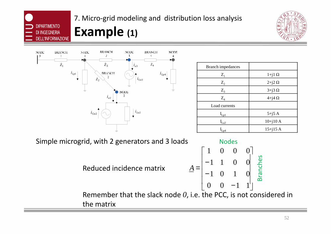
7. Micro-grid modeling and distribution loss analysis
Example (1)
1LpI&
2LaI&2GaI&
3GaI&
3aI&
2aI&
4LpI&
1Z&
2Z&
3Z& 4Z&Branch impedances
Z1 1+j1 Ω
Z2 2+j2 Ω
Z3 3+j3 Ω
Z4 4+j4 Ω
Load currents
ILp1 5+j5 A
52
ILa2 10+j10 A
ILp4 15+j15 A
Simple microgrid, with 2 generators and 3 loads
Reduced incidence matrix
Remember that the slack node 0, i.e. the PCC, is not considered in
the matrix
−−−
=
1100
0101
0011
0001
A
Bra
nch
es
Nodes
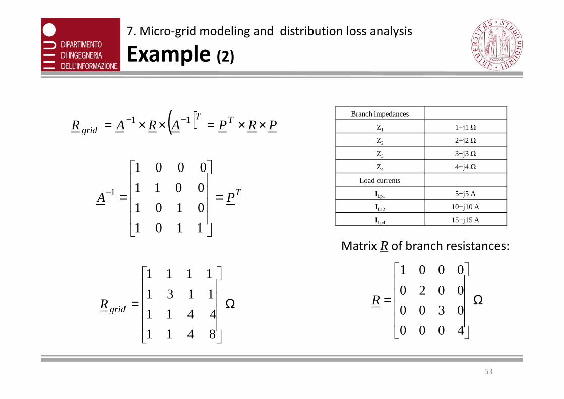
Page 53
( ) PRPARAR TT
grid ××=××= −− 11
7. Micro-grid modeling and distribution loss analysis
Example (2)
TPA =
=− 0 0 1 1
0 0 0 1
1
Branch impedances
Z1 1+j1 Ω
Z2 2+j2 Ω
Z3 3+j3 Ω
Z4 4+j4 Ω
Load currents
ILp1 5+j5 A
53
Matrix Rof branch resistances:
Ω
=
4000
0300
0020
0001
RΩ
=
8 4 1 1
4 4 1 1
1 1 3 1
1 1 1 1
gridR
PA =
=
1 1 0 1
0 1 0 1 ILa2 10+j10 A
ILp4 15+j15 A
Page 54
7. Micro-grid modeling and distribution loss analysis
Example (3)
Branch impedances
Z1 1+j1 Ω
Z2 2+j2 Ω
Z3 3+j3 Ω
Z4 4+j4 Ω
Load currents
ILp1 5+j5 A
Ω
=
8 4 1 1
4 4 1 1
1 1 3 1
1 1 1 1
gridR
54
ILa2 10+j10 A
ILp4 15+j15 A
*grid
Td IRIP && ××=
[ ] W5350
1515
0
1010
55
8 4 1 1
4 4 1 1
1 1 3 1
1 1 1 1
15150101055 =
−
−−
+++=
j
j
j
jjjPd
Page 55
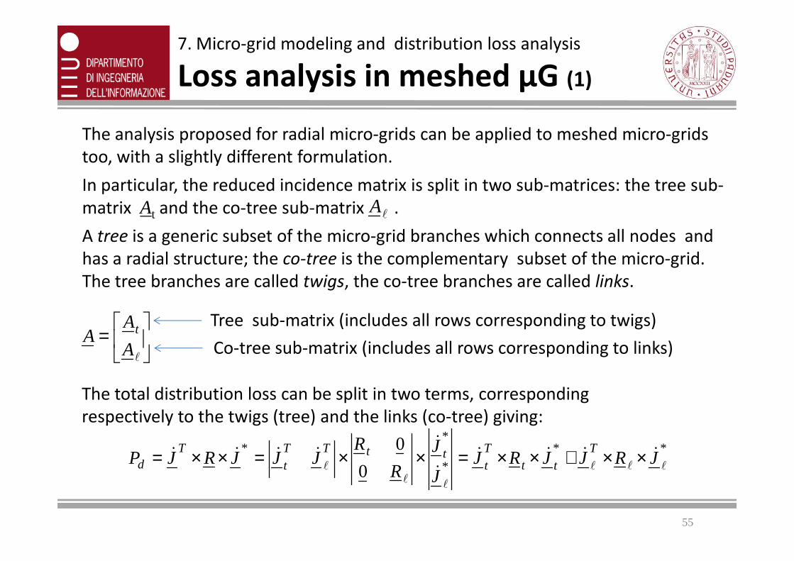
The analysis proposed for radial micro-grids can be applied to meshed micro-grids
too, with a slightly different formulation.
In particular, the reduced incidence matrix is split in two sub-matrices: the tree sub-
matrix At and the co-tree sub-matrix .
A tree is a generic subset of the micro-grid branches which connects all nodes and
has a radial structure; the co-tree is the complementary subset of the micro-grid.
The tree branches are called twigs, the co-tree branches are called links.
7. Micro-grid modeling and distribution loss analysis
Loss analysis in meshed μG (1)
l
A
55
The tree branches are called twigs, the co-tree branches are called links.
=
l
A
AA t
Tree sub-matrix (includes all rows corresponding to twigs)
Co-tree sub-matrix (includes all rows corresponding to links)
The total distribution loss can be split in two terms, corresponding
respectively to the twigs (tree) and the links (co-tree) giving:
*T*tt
Tt*
*ttTT
t*T
d JRJJRJJ
J
R
RJJJRJP
lll
l
l
l
&&&&
&
&
&&&& ××+××=××=××=0
0
Page 56
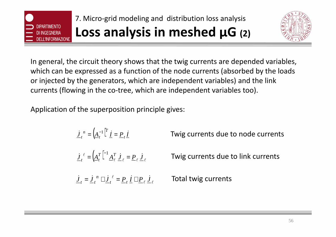
In general, the circuit theory shows that the twig currents are depended variables,
which can be expressed as a function of the node currents (absorbed by the loads
or injected by the generators, which are independent variables) and the link
currents (flowing in the co-tree, which are independent variables too).
Application of the superposition principle gives:
7. Micro-grid modeling and distribution loss analysis
Loss analysis in meshed μG (2)
56
( ) IPIAJ t
T
tn
t&&& == −1
( )llll
l
&&& JPJAAJ TTtt ==
−1
ll
l
&&&&& JPIPJJJ ttn
tt +=+=
Twig currents due to node currents
Twig currents due to link currents
Total twig currents
Page 57
*t
TT*tt
TT*t
Tt
T*tt
Tt
T
*T
J
**tt
J
TTTt
T*T*tt
Ttd
JRPRPJIPRPJJPRPIIPRPI
JRJJPIPRPJPIJRJJRJP
*t
Tt
lllllllll
lll
&
ll
&
lllll
&
43421
&&
43421
&&
43421
&&
43421
&
&&
44 344 21
&&
444 3444 21
&&&&&&
++++=
=+
+
+=+=
Correspondingly, the distribution loss can be rewritten as:
7. Micro-grid modeling and distribution loss analysis
Loss analysis in meshed μG (3)
57
tt
tt
43421434214342143421
l
ll
l
ΩΩΩΩ
( ) *T*tT*tt
Td JRJIJIIP
ll
l
llll
&&&&&& +Ω+Ω+Ω= 2
The distribution loss depends therefore on both node currents and link currents (twig
currents have been removed from the equation).
In practice, also the link currents can be expressed as a function of the node currents,
which distribute among twigs and links depending on their branch impedances.
Since , we can express the equation in the more synthetic form:
Tt
t
Ω=Ω
l
l
Page 58
( ) ( ) IRJJRIJ
P t**td&&&&
&ll
l
llll
l
ll
l
Ω+Ω−=⇒=+Ω+Ω⇒=∂∂ −1
0220
7. Micro-grid modeling and distribution loss analysis
Loss analysis in meshed μG (4)
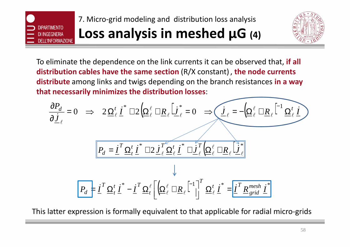
To eliminate the dependence on the link currents it can be observed that, if all
distribution cables have the same section (R/X constant) , the node currents
distribute among links and twigs depending on the branch resistances in a way
that necessarily minimizes the distribution losses:
58
l
( ) *T*tT*tt
Td JRJIJIIP
ll
l
llll
&&&&&& +Ω+Ω+Ω= 2
( ) *meshgrid
T*tT
tT*t
tT
d IRIIRIIIP &&&&&&
ll
l
l
l =Ω
+ΩΩ−Ω=
−1
This latter expression is formally equivalent to that applicable for radial micro-grids
Page 59
Smart micro‐gridsProperties, trends and local control of energy sources
UNICAMP – UNESP, August 2012
Green Technologies enabling Energy Saving
59
8. Optimum control of smart micro‐grids
Page 60
In the basic optimization process, the distribution loss in the micro‐grid is taken
as the quantity to be minimized (cost function). The motivations are:
• This is an optimum choice in terms of energy efficiency
• The power consumption of the micro-grid is minimized
• The currents flowing in the distribution grid are minimized; this implies that:
• The loads are fed by the nearest sources, which corresponds to the most
effective load power sharing among distributed generators
8. Optimum control of smart micro-grids
Optimization goals
60
effective load power sharing among distributed generators
• The voltage drops across the branch impedances are minimized, resulting in a
voltage stabilization effect at all nodes of the micro-grid
The optimization will be firstly done in the assumption that a central controller
drives all energy gateways of the micro-grid and has a complete knowledge of grid
topology and impedances
The results of such optimization are unrealistic, since several other aspects
(mentioned later) should be considered. However, this sets a benchmark to
compare the performances of any other control technique.
Page 61
8. Optimum control of smart micro-grids
Distribution Loss Minimization (1)
Ideal optimization:
• Linear micro-grid modelling
• Grid topology (matrix A) and path impedances (matrix Z) known to the controller
• Unconstrained active and reactive current injection by distributed EPPs
Let IKI
IKI
pp
aa
&&
&&
=
= currents injected at the Na active nodes (energy gateways)
currents absorbed at the Np passive nodes (loads)
61
*grid
Td IRIP &&=
*pp,p
Tp
*pp,a
Ta
*aa,a
Tad IRIIRIIRIP &&&&&& +
ℜ−= 2
Distribution loss:
Optimization goal
Find active node currents Ia that minimize Pd for a given set of load currents Ip
Ta,pp,aT
pgridpp,pTagridpa,p
Tpgridap,a
Tagridaa,a RR
KRKR,KRKR
KRKR,KRKR=
==
==where:
Page 62
00220
0220
0 =−⇒
=−⇒=∂∂
=−⇒=∂∂
⇒=∂∂
pp,aaa,a
p,aa,ad
p,aa,ad
a
d IRIRbRyR
y
P
aRxRx
P
I
P&&
&
yjxI a +=& bjaI p +=&
pp,aa,aopt,a IRRI &&1−=
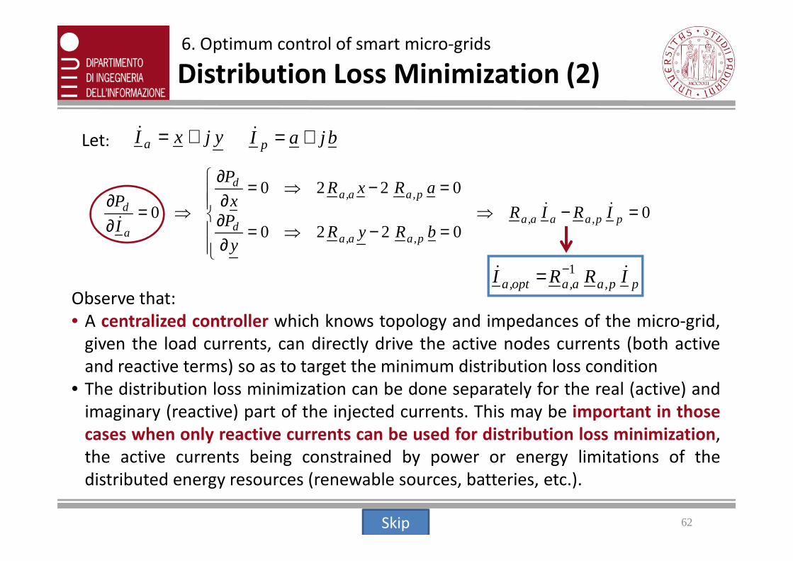
6. Optimum control of smart micro-grids
Distribution Loss Minimization (2)
Let:
62
pp,aa,aopt,a IRRI && =Observe that:
• A centralized controller which knows topology and impedances of the micro-grid,
given the load currents, can directly drive the active nodes currents (both active
and reactive terms) so as to target the minimum distribution loss condition
• The distribution loss minimization can be done separately for the real (active) and
imaginary (reactive) part of the injected currents. This may be important in those
cases when only reactive currents can be used for distribution loss minimization,
the active currents being constrained by power or energy limitations of the
distributed energy resources (renewable sources, batteries, etc.).
Skip
Page 63
8. Optimum control of smart micro-grids
Application example (1)
1LpI&
2LaI&2GaI&
3GaI&
3aI&
2aI&
4LpI&
1Z&
2Z&
3Z& 4Z&Branch impedances
Z1 1+j1 Ω
Z2 2+j2 Ω
Z3 3+j3 Ω
Z4 4+j4 Ω
Load currents
ILp1 5+j5 A
63
Lp1
ILa2 10+j10 A
ILp4 15+j15 A
Simple microgrid, with 2 generators and 3 loads
STEP 1: Reduced incidence matrix
−−−
=
1100
0101
0011
0001
A
Bra
nch
es
Nodes
Page 64
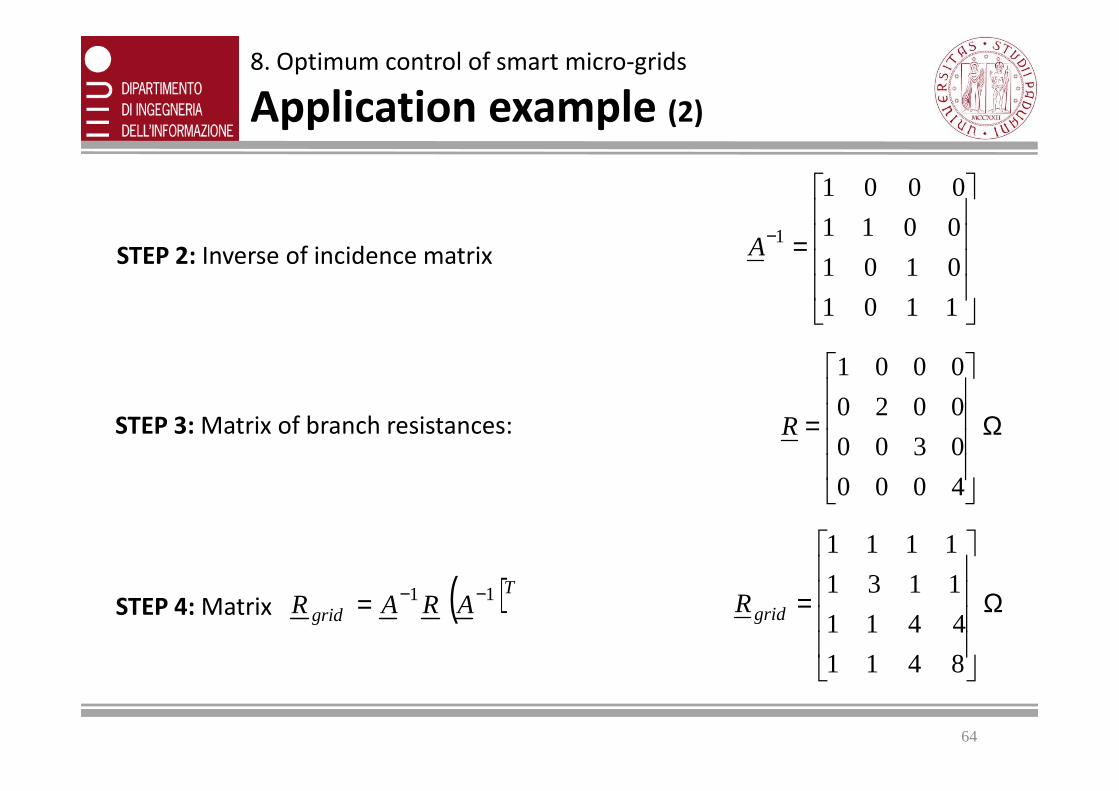
0020
0001
8. Optimum control of smart micro-grids
Application example (2)
=−
1 1 0 1
0 1 0 1
0 0 1 1
0 0 0 1
1ASTEP 2: Inverse of incidence matrix
64
STEP 3: Matrix of branch resistances: Ω
=
4000
0300
0020R
( )Tgrid ARAR 11 −−=STEP 4: Matrix Ω
=
8 4 1 1
4 4 1 1
1 1 3 1
1 1 1 1
gridR
Page 65
Given the above matrices, the inherent distribution loss (with all inverters switched
off) can be derived as a function of load currents IL:
[ ] W5350
1515
0
1010
55
8 4 1 1
4 4 1 1
1 1 3 1
1 1 1 1
15150101055 =
−
−−
+++==
j
j
j
jjjIRIP*Lgrid
TLdo
&&
8. Optimum control of smart micro-grids
Application example (3)
65
15158 4 1 1 − j
STEP 5: Matrices Ka and Kp (identify
active and passive nodes
=
=
1 0 0 0
0 0 0 1
0 1 0 0
0 0 1 0pa KK
=
=
=
=
81
11
41
11
41
11
41
13
p,pa,p
p,aa,a
R,R
R,R
STEP 6: Sub-matrices of Rgrid
Tpgridpp,p
Tagridpa,p
Tpgridap,a
Tagridaa,a
KRKR,KRKR
KRKR,KRKR
==
==
Page 66
−−−−
=
++
==
−−
909115909115
1.36261.3636
1515
55
41
11
41
131
1
.j.
j
j
jIRRI pp,aa,aopt,a&&
STEP 7: Calculation of the optimum currents to be
injected at the active nodes given the currents Ip
absorbed by the loads at the passive grid nodes. Let:
The optimum currents are:
8. Optimum control of smart micro-grids
Application example (4)
++
=
=
1515
55
4
1
j
j
I
II
Lp
Lpp
&
&
&
66
++
=
−−−−
−
+=⇒
−−
=909115909115
11.362611.3636
909115909115
1.36261.3636
0
1010
3
2
33
22
.j.
j
.j.
jj
I
I
II
III
Ga
Ga
GaLa
GaLaa
&
&
&&
&&
&
In practice, currents Ia can be expressed as the difference between the currents
absorbed by the loads connected at the active grid nodes (ILa) and the currents
injected by the distributed energy resources at the same nodes (IGa). Thus:
STEP 8: Calculation of the distribution loss in the optimum condition
1827.3W2 =+
ℜ+= *
pp,pTp
*pp,a
Ta
*aa,a
Taopt,d IRIIRIIRIP &&&&&&
Page 67
8. Optimum control of smart micro-grids
Remarks
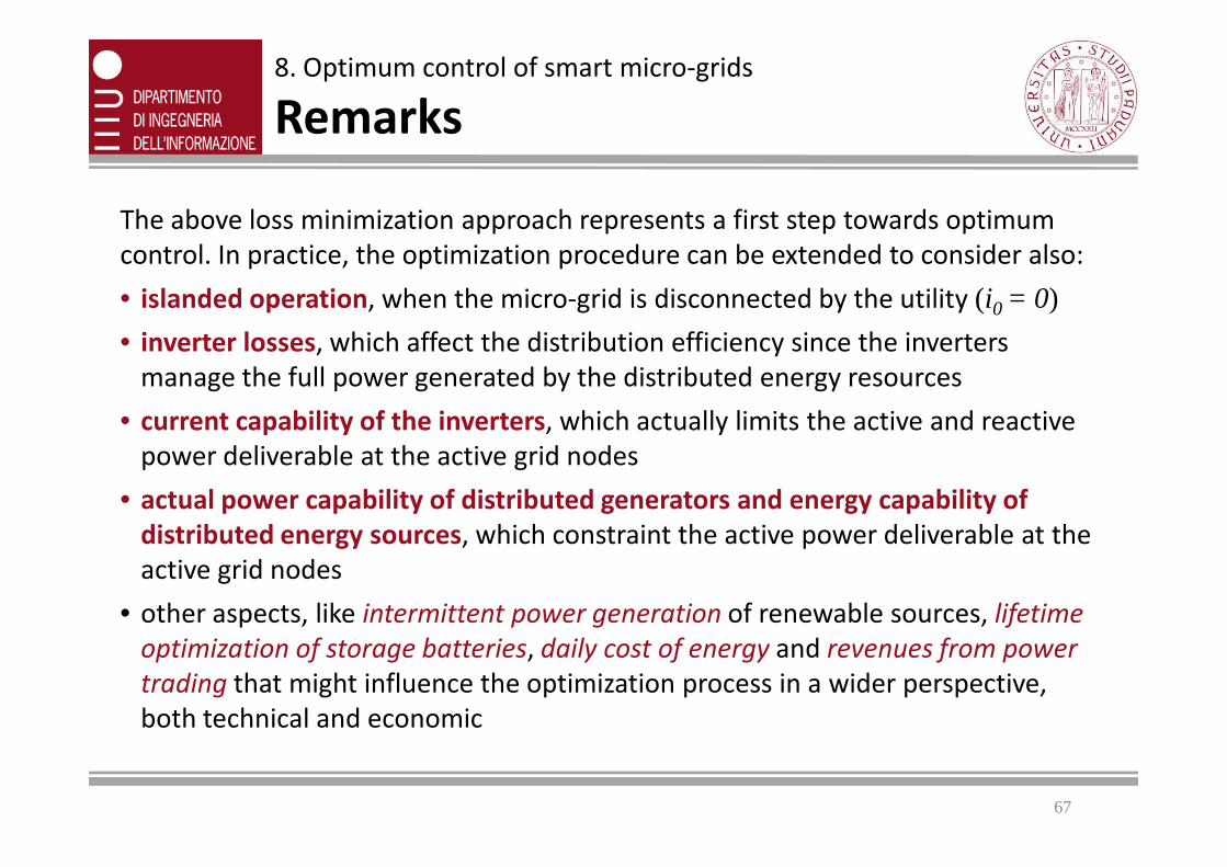
The above loss minimization approach represents a first step towards optimum
control. In practice, the optimization procedure can be extended to consider also:
• islanded operation, when the micro-grid is disconnected by the utility (i0 = 0)
• inverter losses, which affect the distribution efficiency since the inverters
manage the full power generated by the distributed energy resources
• current capability of the inverters, which actually limits the active and reactive
67
• current capability of the inverters, which actually limits the active and reactive
power deliverable at the active grid nodes
• actual power capability of distributed generators and energy capability of
distributed energy sources, which constraint the active power deliverable at the
active grid nodes
• other aspects, like intermittent power generation of renewable sources, lifetime
optimization of storage batteries, daily cost of energy and revenues from power
trading that might influence the optimization process in a wider perspective,
both technical and economic
Page 68
Smart micro‐gridsProperties, trends and local control of energy sources
UNICAMP – UNESP, August 2012
Green Technologies enabling Energy Saving
68
9. On‐line Identification of micro‐grid parameters
Page 69
The previous optimization has been done in the assumption that a central controller
has a complete knowledge of grid topology and impedances.
In this section we analyze some techniques which allow on‐line evaluation of node‐
to‐node distances and identification of micro‐grid topology.
These techniques take advantage of the capabilities of modern powerline
communication (PLC) technologies, which are particularly suited for micro-grid
applications.
In fact, in low-voltage residential micro-grids, the same power lines connecting the
9. On-line Identification of micro-grid parameters
Identification goals
69
In fact, in low-voltage residential micro-grids, the same power lines connecting the
users can be used to convey data. The small distances between users and the
absence of transformers make possible a direct powerline communication among
grid nodes, without requiring any additional communication infrastructure.
The on-line identification approach can also be extended to estimate the line
impedances.
However, in a residential micro-grid the size of the distribution cables is usually the
same, thus the knowledge of node-to-node distances is sufficient to run the optimum
control algorithm, as well as the distributed quasi-optimum control techniques
which will be discussed in the next sections.
Skip
Page 70
• Node-to-node communication architecture
• Node-to-node distance measurement
Standard PRIME
(PoweRline Intelligent
Metering Evolution)
PRIME overview:
• Designed for outdoor applications
• OFDM physical layer
• Maximum bit rate 128kbps
9. On-line Identification of micro-grid parameters
Node‐to‐node communication
70
• Maximum bit rate 128kbps
• Transmission over CENELEC A band, in
the range 45kHz-92kHz with 97 equally
spaced sub-carriers
• MAC layer needs to be “customized” to
fit peer-to-peer communication (PRIME
is originally master-slave)
Node-to-node distance measurement: PLC enables the use of TOA (Time Of
Arrival) techniques, currently under testing over ≈1km of real distribution
cables in the Smart Micro-Grid Facility at DEI
Symbols=OFDM 288bits
symbols – M<64
Page 71
9. On-line Identification of micro-grid parameters
Node‐to node distance measurement
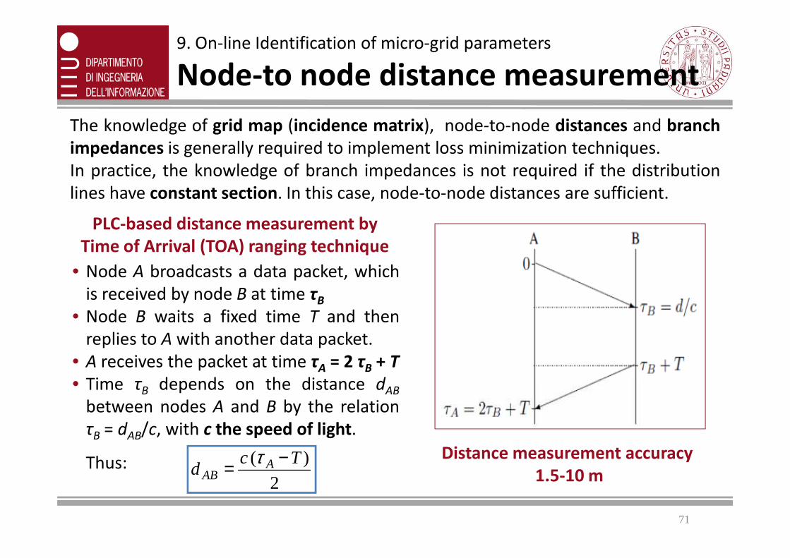
The knowledge of grid map (incidence matrix), node-to-node distances and branch
impedances is generally required to implement loss minimization techniques.
In practice, the knowledge of branch impedances is not required if the distribution
lines have constant section. In this case, node-to-node distances are sufficient.
• Node A broadcasts a data packet, which
PLC‐based distance measurement by
Time of Arrival (TOA) ranging technique
71
• Node A broadcasts a data packet, which
is received by node B at time τB
• Node B waits a fixed time T and then
replies to A with another data packet.
• A receives the packet at time τA = 2 τB + T
• Time τB depends on the distance dAB
between nodes A and B by the relation
τB = dAB/c, with c the speed of light.
Thus:2
)( Tcd A
AB−= τ Distance measurement accuracy
1.5‐10 m
Page 72
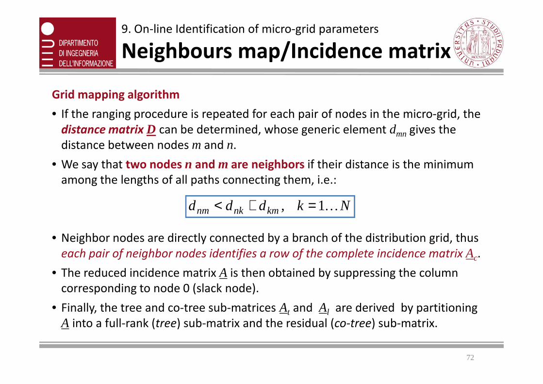
Grid mapping algorithm
• If the ranging procedure is repeated for each pair of nodes in the micro-grid, the
distance matrix D can be determined, whose generic element dmn gives the
distance between nodes mand n.
• We say that two nodes n and m are neighbors if their distance is the minimum
among the lengths of all paths connecting them, i.e.:
9. On-line Identification of micro-grid parameters
Neighbours map/Incidence matrix
72
• Neighbor nodes are directly connected by a branch of the distribution grid, thus
each pair of neighbor nodes identifies a row of the complete incidence matrix Ac.
• The reduced incidence matrix A is then obtained by suppressing the column
corresponding to node 0 (slack node).
• Finally, the tree and co-tree sub-matrices At and Al are derived by partitioning
A into a full-rank (tree) sub-matrix and the residual (co-tree) sub-matrix.
Nk,ddd kmnknm K1=+<
Page 73
Smart micro‐gridsProperties, trends and local control of energy sources
UNICAMP – UNESP, August 2012
Green Technologies enabling Energy Saving
73
10. Distributed surround control of smart micro‐grids
Page 74
• In this section we analyze a distributed plug & play control technique, called
surround control, which provides local minimization of the distribution losses,
resulting in a quasi-optimum operation of the entire micro-grid.
• The technique requires that every grid node, both active and passive, is equipped
with a smart meter, i.e., a local measurement unit capable of data processing and
powerline communication.
• This allows identification of both the incidence matrix (network topology) and the
10. Distributed surround control
Introduction
• This allows identification of both the incidence matrix (network topology) and the
distance matrix (node-to-node distances), extended to active and passive nodes.
• Given the incidence matrix, each active node identifies the neighbor nodes, i.e., the
active nodes connected by a direct link and the passive nodes fed by such links.
• Then, a local optimum control algorithm is applied, which only requires data
exchange among neighbor nodes.
• The proposed control technique ensures flexibility and scalability, i.e., it can be
applied irrespective of micro-grid architecture, and automatically adapts when a
new node is implemented in the micro-grid.
74
Page 75
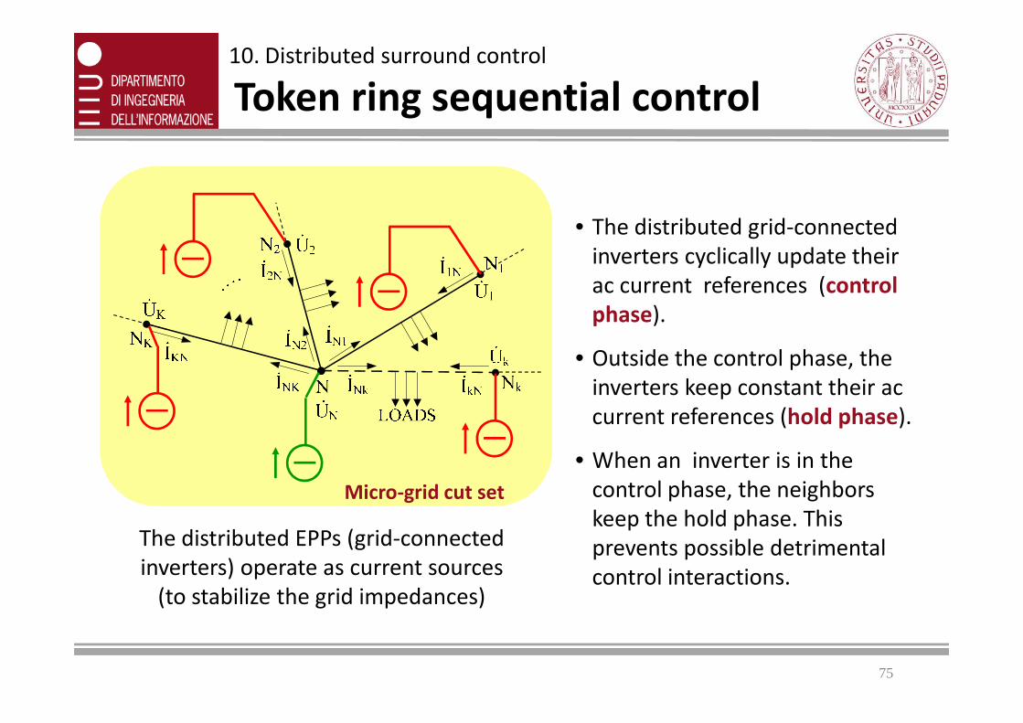
• The distributed grid-connected
inverters cyclically update their
ac current references (control
phase).
• Outside the control phase, the
10. Distributed surround control
Token ring sequential control
• Outside the control phase, the
inverters keep constant their ac
current references (hold phase).
• When an inverter is in the
control phase, the neighbors
keep the hold phase. This
prevents possible detrimental
control interactions.
The distributed EPPs (grid-connected
inverters) operate as current sources
(to stabilize the grid impedances)
Micro‐grid cut set
75
Page 76
Let rAB be the resistance per
unit of length of the line, the
distribution loss in the line
between active nodes A and
B is given by:
10. Distributed surround control
Conduction loss in distribution lines
∑ =∆=K
kkABLOSS IrP2
&
Given the currents absorbed by the passive loads fed
along path A-B, the distribution loss in path A-B can
therefore be expressed as a function of active node
current IAB (or IBA).
∑
∑
=
=
∆=
=∆=
K
k
*kkkAB
kkkABLOSS
IIr
IrP
0
0
&&
&
−−=
−=
∑
∑
+=
=K
kLBAk
k
LABk
III
III
1
1
l
l
l
l
&&&
&&&
where:
Distribution path connecting active nodes A and B
76
Page 77
Optimization goal: find the
values of IAB and IBA that
minimize the conduction
losses in path A-B
10. Distributed surround control
Loss minimization in distribution lines (1)
00 =∂
∂=
∂∂ LOSSLOSS
I
P
I
P&&
The optimum node
currents depend only on
the loads and their
distribution along path
A-B
Moreover:
Distribution path connecting active nodes A and B
∂∂ BAAB II &&
=
=
∑
∑
=
=K
kAkkL
AB
optBA
K
kBkkL
AB
optAB
dId
I
dId
I
1
1
1
1
&&
&&
BAoptBABA
optABAB UU
II
II&&
&&
&&
=⇔
==
77
Page 78
10. Distributed surround control
Loss minimization in distribution lines (2)
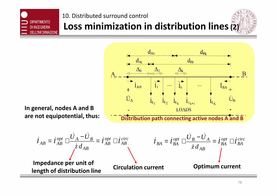
In general, nodes A and B
are not equipotential, thus:
Impedance per unit of
length of distribution lineCirculation current Optimum current
Distribution path connecting active nodes A and B
circAB
optAB
AB
BAoptABAB II
dz
UUII &&
&
&&
&& +=−+= circBA
optBA
AB
ABoptBABA II
dz
UUII &&
&
&&
&& +=−+=
78
Page 79
4434421
&
&&
321
&&&
&&circN
optN I
K
k k
kN
I
K
k
optkN
K
kkNN
Z
UUIII ∑∑∑
===
−+==
111
The current at node N can be expressed
as:
10. Distributed surround control
Loss minimization in cut sets (2)
Consider a cut-set of the micro-grid
Depends on
loads connected
to paths L1 - LK
Depends on voltage
differences
Minimum distribution loss condition
==
=⇒=
∑∑==
K
k k
K
k k
koptNN
optNN
circN
ZZ
UUU
III
11
10&&
&
&&
&&
&EPP in control phase
EPPs in hold phase
Micro‐grid cut set
79
Page 80
The computation of optimum node
current (EPP reference current)
requires distance estimation
(ranging), local grid mapping, and
current measurement at
surrounding passive nodes)
This equation holds separately for active and
reactive terms , thus optimization can be
done by acting on active currents, reactive
10. Distributed surround control
Node current/voltage optimization
∑ ∑∑= ==
===K
k
M
m
Nkm
NkL
Nk
K
k
optNk
optNN
Nk
mdI
dIII
1 11
1&&&&
Node current optimization
The computation of optimum node
voltage (EPP reference voltage)
requires local grid mapping,
knowledge of path impedances (or
node-to-node distances), and
voltage measurement at
surrounding active nodes
done by acting on active currents, reactive
currents, or both
∑
∑
∑
∑
=
=
=
= ≈==K
k k
K
k k
k
K
k k
K
k k
k
optNN
d
d
U
Z
Z
U
UU
1
1
1
1
11
&
&
&
&
&&
Node voltage optimization
This method is very sensitive to voltage
measurement errors
80
Page 81
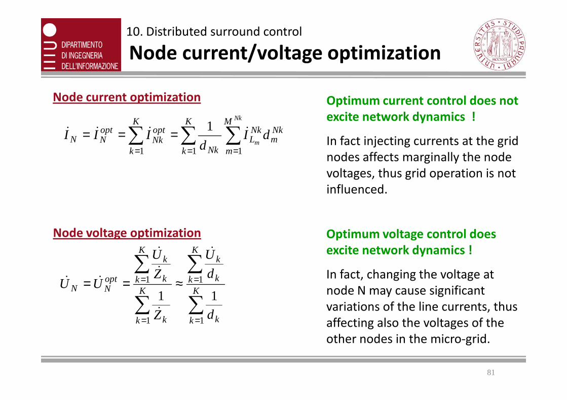
10. Distributed surround control
Node current/voltage optimization
∑ ∑∑= ==
===K
k
M
m
Nkm
NkL
Nk
K
k
optNk
optNN
Nk
mdI
dIII
1 11
1&&&&
Node current optimization Optimum current control does not
excite network dynamics !
In fact injecting currents at the grid
nodes affects marginally the node
voltages, thus grid operation is not
influenced.
∑
∑
∑
∑
=
=
=
= ≈==K
k k
K
k k
k
K
k k
K
k k
k
optNN
d
d
U
Z
Z
U
UU
1
1
1
1
11
&
&
&
&
&&
Node voltage optimization
81
Optimum voltage control does
excite network dynamics !
In fact, changing the voltage at
node N may cause significant
variations of the line currents, thus
affecting also the voltages of the
other nodes in the micro-grid.
Page 82
∑=−
−=
K
k NkoptNN
optNN
dII
UUz
1
1&&
&&
&
KeqN d
zZ &
&
=−
∑1
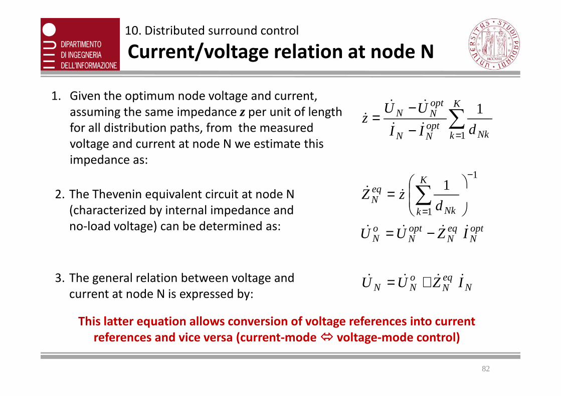
12. The Thevenin equivalent circuit at node N
1. Given the optimum node voltage and current,
assuming the same impedance z per unit of length
for all distribution paths, from the measured
voltage and current at node N we estimate this
impedance as:
10. Distributed surround control
Current/voltage relation at node N
optN
eqN
optN
oN
k NkN
IZUU
dzZ
&&&&
&
−=
=
=∑
1
2. The Thevenin equivalent circuit at node N
(characterized by internal impedance and
no-load voltage) can be determined as:
3. The general relation between voltage and
current at node N is expressed by:N
eqN
oNN IZUU &&&& +=
This latter equation allows conversion of voltage references into current
references and vice versa (current‐mode voltage‐mode control)
82
Page 83
NI&
NNU&
1U&
2U&
kU&
KU&
1NZ&
2NZ&NkZ&
NKZ&
Token ring control
• A token moves along the micro-grid, and only the
active node (N) keeping the token is enabled to
modify its current reference according to the
minimum distribution loss criterion
10. Distributed surround control
Surround control implementation
83
• When an active node receives the token, it:
1. collects voltage phasors from neighbour nodes
2. measures (or recalls) the distances from
neighbour nodes
3. computes the optimum voltage reference
4. computes the current reference variation
needed to reach the optimum voltage
5. sends the token to the next active node
∑∑==
≈K
k Nk
K
k Nk
koptN dd
UU
11
1&
&
eqN
NoptN
NZ
UUI
&
&&
&
−=∆
Page 84
NI&
NNU&
1U&
2U&
kU&
KU&
1NZ&
2NZ&NkZ&
NKZ&
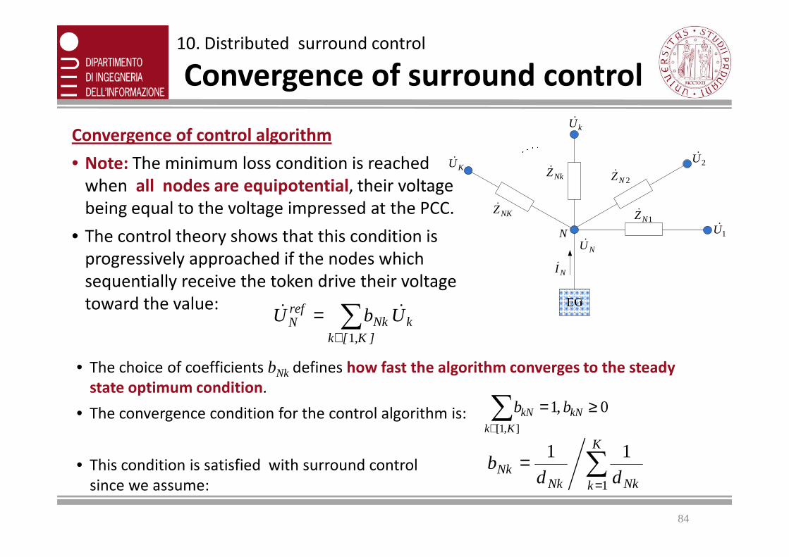
Convergence of control algorithm
• Note: The minimum loss condition is reached
when all nodes are equipotential, their voltage
being equal to the voltage impressed at the PCC.
• The control theory shows that this condition is
progressively approached if the nodes which
sequentially receive the token drive their voltage
10. Distributed surround control
Convergence of surround control
• The choice of coefficients bNk defines how fast the algorithm converges to the steady
state optimum condition.
• The convergence condition for the control algorithm is:
• This condition is satisfied with surround control
since we assume:
84
sequentially receive the token drive their voltage
toward the value:k
]K,[kNk
refN UbU && ∑
∈=
1
0 ,1],1[
≥=∑∈
kN
Kk
kN bb
∑=
=K
k NkNkNk dd
b1
11
Page 85
Smart micro‐gridsProperties, trends and local control of energy sources
UNICAMP – UNESP, August 2012
Green Technologies enabling Energy Saving
85
11. Distributed cooperative control of smart micro‐grids
Page 86
Surround Control ensures minimum distribution loss, but requires a
full knowledge of the micro-grid topology, which requires data
exchange among all grid nodes.
Moreover, it has strict requirements in terms of node-to-node
communication and synchronization (PMU, Phasor Measurement
Unit), which are not easily satisfied with cheap commercial technology.
11. Distributed cooperative control
Introduction to cooperative control
86
Question: there is a different distributed control technique which has
easier implementation and still keeps good performances?
(Sub‐optimum solution)
Remark: Beyond the mathematical analysis, an intuitive interpretation
of distribution loss minimization is that “the distribution loss reduces if
the loads are supplied by the generators nearby”
Page 87
Cooperative control approach
1. Each load msplits its active and reactive power demand Pm and Qm among
the active nodes n in inverse proportion to their distances:
m
N
n
nmn
m
eqm
m
N
nnm
nm
mnm PP
d
dP
dd
PP =⇒=
= ∑∑
=
−
= 1
1
0
1
43421
11. Distributed cooperative control
Principle of cooperative control
87
2. Each active node n, within its current capability, supplies the total power
requested by the passive loads:
m
N
n
nmn
m
eqm
m
N
nnm
nm
mnm
d
QQd
dQ
dd
QQ
eqm
=⇒=
= ∑∑
=
−
= 1
1
0
1
43421
∑∑∑∑====
====M
mnm
eqm
m
M
m
nmn
M
mnm
eqm
m
M
m
nmn
d
dQQQ
d
dPPP
1111
Page 88
11. Distributed cooperative control
Pros & cons of cooperative control
Advantages of cooperative control• Use of PMUs (phasor measurement units) can be avoided, since the loads
address their requests in terms of active and reactive power, which are
conservative quantities and do not depend on the phase of the node voltages.
• There is no need for micro-grid topology identification, since only the node-to-
node distances are requested to implement the control algorithm.
88
Disadvantage of cooperative control• The solution can diverge from the optimum condition in case of saturation of
the current capability of the inverters.
Upgrade of cooperative control• The saturation conditions must be properly managed by shifting the power
requests from the saturated active nodes to the non-saturated nodes.
Skip
Page 89
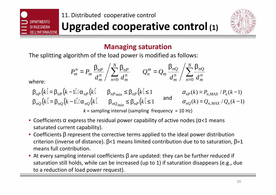
Managing saturationThe splitting algorithm of the load power is modified as follows:
11. Distributed cooperative control
Upgraded cooperative control (1)
∑∑==
ββ=ββ=
N
nnm
nQnm
nQm
mn
N
nnm
nPnm
nPm
nm
ddQQ
ddPP
00
( ) ( ) ( ) ( )( ) ( ) ( ) ( )
11
≤β≤βα⋅−β=β≤β≤βα⋅−β=β kkkk nPminnPnPnPnP )1(/)( ,
−=−= kPPk nMAXnnP
αα
where:
and
89
k = sampling interval (sampling frequency = 10 Hz)
( ) ( ) ( ) ( ) 11 ≤β≤βα⋅−β=β kkkk nPminnQnQnQnQ )1(/)( , −= kQQk nMAXnnQαand
• Coefficients α express the residual power capability of active nodes (α<1 means
saturated current capability).
• Coefficients β represent the corrective terms applied to the ideal power distribution
criterion (inverse of distance). β<1 means limited contribution due to to saturation, β=1
means full contribution.
• At every sampling interval coefficients β are updated: they can be further reduced if
saturation still holds, while can be increased (up to 1) if saturation disappears (e.g., due
to a reduction of load power request).
Page 90
11. Distributed cooperative control
Upgraded cooperative control (2)
Managing saturationThe splitting algorithm of the load power is modified as follows:
∑∑==
ββ=ββ=
N
nnm
nQnm
nQm
mn
N
nnm
nPnm
nPm
nm
ddQQ
ddPP
00
( ) ( ) ( ) ( )( ) ( ) ( ) ( )
11
≤β≤βα⋅−β=β≤β≤βα⋅−β=β kkkk nPminnPnPnPnP )1(/)( ,
−=−= kPPk nMAXnnP
αα
where:
and
90
Advantages• The power limits of the active nodes are automatically met
• Recovery from saturation happens quickly
• Load power requests are met precisely
• The power splitting criterion approaches the “minimum distance” criterion as
close as possible, within the power limits of the active nodes
• Control is inherently stable
( ) ( ) ( ) ( ) 11 ≤β≤βα⋅−β=β kkkk nPminnQnQnQnQ )1(/)( , −= kQQk nMAXnnQαand
Page 91
Smart micro‐gridsProperties, trends and local control of energy sources
UNICAMP – UNESP, August 2012
Green Technologies enabling Energy Saving
91
12. Simulation results
Page 92
Assumptions
• The proposed control techniques have been validated
by simulation in the Matlab – Simulink environment.
• To minimize the complexity of simulation and to
reduce the simulation times a phasorial simulation
12. Simulation results
Simulation approach
reduce the simulation times a phasorial simulation
tool has been developed.
• The graphs showing the time behaviour of the system
represent must be interpreted as sequences of steady
states (quasi-stationary behavior), where fast
dynamics are neglected.
92
Page 93
DG PMAX
kW
SMAX
kVA
G1 1 2
G2 1 2
G3 3 5
G4 3 5
G5 3 5
G6 1 2
Load Z=R+jωL Power @
230VRMS
L1 5kW cosφ=0.91
L2 5kW cosφ=0.91
L3 2.5kW cosφ=0.96
L4 2.5kW cosφ=0.96
L5 2.5kW cosφ=0.96
L6 5kW cosφ=0.910230 ∠= VV
feeder ..VM
lResidentia
0N
1N
2N
3N
4N5N
6N
7N 8N
9N 10N
1B 2B
3B
4B
6B 5B
7B8B
9B 10B
2L
3L
4L
5L
1G
2G
3G
4G
5G
18‐bus LV network
12. Simulation results
Simulation Example (1)
G6 1 2
G7 10 15
G8 10 15
G9 10 15
L7 10kW cosφ=0.80
L8 10kW cosφ=0.80
L9 10kW cosφ=0.80
0230 ∠= RMSph VV
Workshop
11N
12N13N
14N
15N16N
17N
18N
11B
12B
13B14B 15B 16B
17B
18B
1L
6L
7L 8L
9L
1G
6G
7G 8G
9G
kWPRL 5.52= 0.857 cos =RLϕ
kWPRG 55= kVASRG 85=
Total Loads
Total DERs
/ EPPs
2240mmS=r = 0.08Ω/kml = 255µH/kmΦ = π/4 rad Total length of distribution line 1.8km
93
Page 94
Initial situation: Inverters OFF
1.2kWmax
=RPLoss:
Voltages:
1Generators nodes voltages - RMS value
12. Simulation results
Simulation Example (2)
The distributed control techniques are analyzed in specific
operating conditions, their performance being compared
with those of optimum control.
Two cases are considered:
• Active and Reactive current control constrained only by
converters saturation (to show the achievable
performances in a real system with power generation &
energy storage)
0 1 2 3 4 5 6 7 8 90.94
0.95
0.96
0.97
0.98
0.99
Generator n°
p.u.
energy storage)• In practice, actual active power capability is determined by
energy storage & generated power constraints (sun, wind,
batteries, etc), while reactive power can be regulated within
the current capability of the inverters.
• Purely reactive current control constrained by converters
saturation (to show the achievable improvement without
power generation & energy storage)
The actual micro‐grid performances are intermediate
between these two cases
94
Page 95
12. Simulation results
Surround control (1)
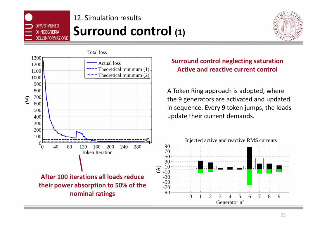
Surround control neglecting saturation
Active and reactive current control
A Token Ring approach is adopted, where
the 9 generators are activated and updated
in sequence. Every 9 token jumps, the loads
update their current demands.400500600700800900
1000110012001300
Total loss
(W)
Actual lossTheoretical minimum (1)Theoretical minimum (2)
95
After 100 iterations all loads reduce
their power absorption to 50% of the
nominal ratings
update their current demands.
0 1 2 3 4 5 6 7 8 9-90-70-50-30-101030507090
Injected active and reactive RMS currents
(A)
Generator n°
0 40 80 120 160 200 240 2800
100200300400
Token Iteration
4511
Page 96
12. Simulation results
Surround control (2)
500600700800900
1000110012001300
Total loss
(W)
Actual lossTheoretical minimum (1)Theoretical minimum (2)
A Token Ring approach is adopted, where
the 9 generators are activated and updated
in sequence. Every 9 token jumps, the loads
update their current demands.
Surround control considering saturation
Active and reactive current control
96
0 1 2 3 4 5 6 7 8 9-90-70-50-30-101030507090
Injected active and reactive RMS currents
(A)
Generator n°
After 100 iterations all loads reduce
their power absorption to 50% of the
nominal ratings
0 40 80 120 160 200 240 2800
100200300400500
Token Iteration
11624
update their current demands.
Page 97
Cooperative control without
saturation management
Active and reactive current control
12. Simulation results
Cooperative Control (1)
A Token Ring approach is adopted, where
the 9 generators are activated and updated
in sequence. Every 9 token jumps, the loads
update their current demands.400500600700800900
1000110012001300
Total loss
(W)
Actual lossTheoretical minimum (1)Theoretical minimum (2)
0 1 2 3 4 5 6 7 8 9-90-70-50-30-101030507090
Injected active and reactive RMS currents
(A)
Generator n°
Active
ReactiveAfter 100 iterations all loads reduce
their power absorption to 50% of the
nominal ratings
update their current demands.
0 20 40 60 80 100 120 140 160 180 2000
100200300400
Token Iteration
11624
97
Page 98
Cooperative control with
Saturation Management
Active and reactive current control
-30-101030507090
Injected active and reactive RMS currents
(A)
Without management
12. Simulation results
Cooperative control (2)
400500600700800900
1000110012001300
Total loss
(W)
Actual lossTheoretical minimum (1)Theoretical minimum (2)
0 1 2 3 4 5 6 7 8 9-90-70-50-30-101030507090
Injected active and reactive RMS currents
(A)
Generator n°
0 1 2 3 4 5 6 7 8 9-90-70-50-30-10
Generator n°
With management
0 1 2 3 4 5 6 7 8 9-90-70-50-30-101030507090
Ideal Injected active and reactive RMS currents
(A)
Generator n°
Theoretical Optimum
0 20 40 60 80 100 120 140 160 180 2000
100200300400
Token Iteration
11624
98
Page 99
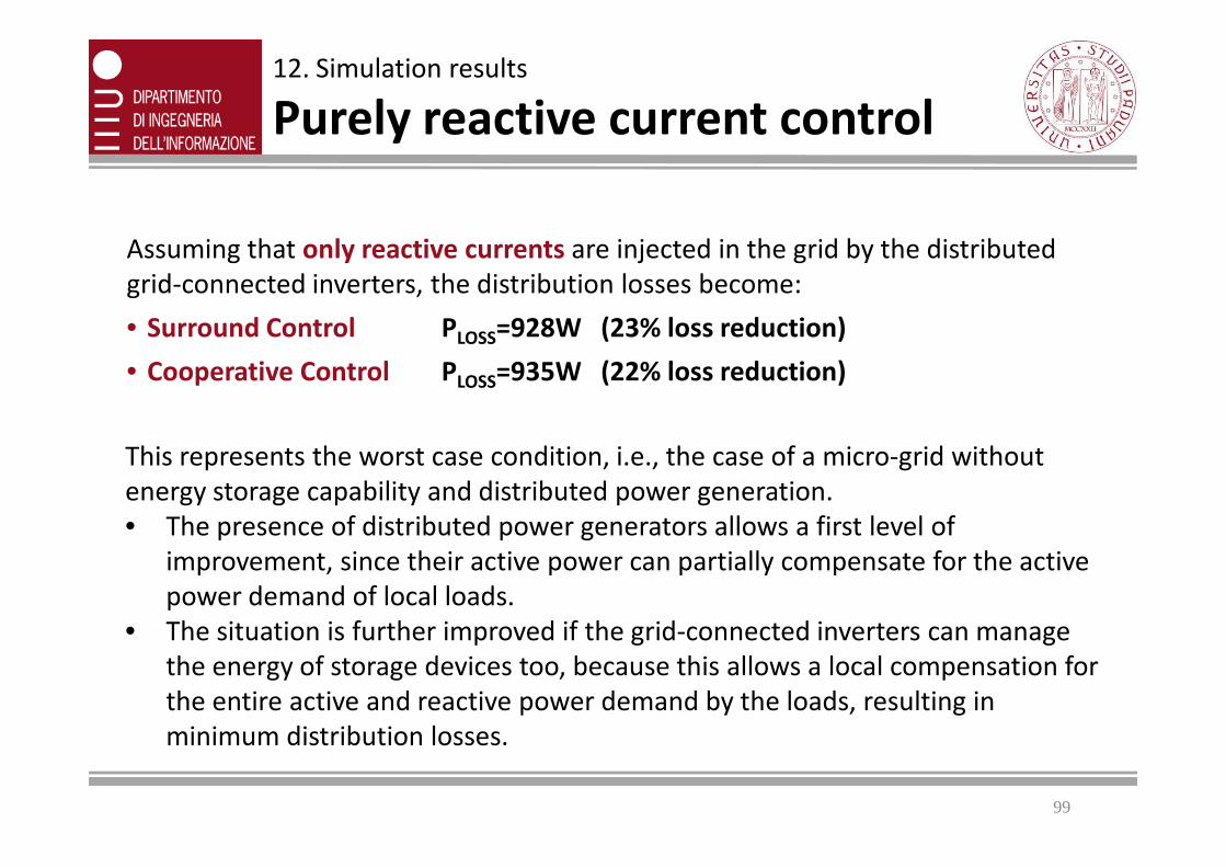
Assuming that only reactive currents are injected in the grid by the distributed
grid-connected inverters, the distribution losses become:
• Surround Control PLOSS=928W (23% loss reduction)
• Cooperative Control PLOSS=935W (22% loss reduction)
12. Simulation results
Purely reactive current control
99
This represents the worst case condition, i.e., the case of a micro-grid without
energy storage capability and distributed power generation.
• The presence of distributed power generators allows a first level of
improvement, since their active power can partially compensate for the active
power demand of local loads.
• The situation is further improved if the grid-connected inverters can manage
the energy of storage devices too, because this allows a local compensation for
the entire active and reactive power demand by the loads, resulting in
minimum distribution losses.
Page 100
12. Simulation results
Purely reactive current control
400500600700800900
1000110012001300
Total loss
(W)
928
Current lossTheoretical minimum (1)Theoretical minimum (2)
Cooperative control with
Saturation Management
(pure reactive current control)
100
0 20 40 60 80 100 120 140 160 180 2000
100200300400
Token Iteration
230
After 100 iterations all loads reduce
their power absorption to 50% of the
nominal ratings
0 1 2 3 4 5 6 7 8 9-90-70-50-30-101030507090
Injected active and reactive RMS currents
(A)
Generator n°
Page 101
Conclusions1. Smart micro-grids represent a fast-growing and challenging arena for ICT,
power electronics and power systems research and applications
2. The bottom-up revolution made possible by an extensive implementation of
the micro-grid paradigm can have a dramatic impact on the entire value chain
of the electrical market
3. A structured multi-layer reorganization of the electrical grid can provide huge
Smart micro‐gridsProperties, trends and local control of energy sources
101
3. A structured multi-layer reorganization of the electrical grid can provide huge
benefits in terms of energy savings, quality of service and flexibility of
operation, without altering the physical infrastructure of the grid
4. The development of suitable distributed control & communication
techniques can provide flexibility, scalability, power quality, integration and
exploitation of any kind of energy resources, energy efficiency and stability of
operation
5. The successful Internet paradigm can possibly be replicated in the domain of
distributed energy generation, distribution and utilization
Page 102
Smart micro‐gridsProperties, trends and local control of energy sources
UNICAMP – UNESP, August 2012
Green Technologies enabling Energy Saving
102
Research activities at DEI/UniPD
DEI team
DEI smart grid facility