applied sciences

Article

Micro-Mechanism of Spherical Gypsum ParticleBreakage under Ball–Plane Contact Condition

Shicai Yu 1,2, Mincai Jia 1,2,*, Jian Zhou 1,2, Cheng Zhao 1,2 and Lin Li 1,2

1 Department of Geotechnical Engineering, Tongji University, Shanghai 200092, China;catfish.yu@outlook.com (S.Y.); tjugezhoujian@tongji.edu.cn (J.Z.); 09184@tongji.edu.cn (C.Z.);1710204@tongji.edu.cn (L.L.)

2 Key Laboratory of Geotechnical and Underground Engineering, Ministry of Education, Tongji University,Shanghai 200092, China

* Correspondence: mincai_jia@tongji.edu.cn

Received: 14 October 2019; Accepted: 6 November 2019; Published: 9 November 2019�����������������

Abstract: Coarse-grained soils are used extensively in engineering applications. The breakage ofcoarse-grained soil particles may have a great effect on their mechanical characteristics. It is importantto fully understand the phenomenon of particle breakage and comprehend its effect on engineeringproperties. The aim of this study was to investigate the process and mechanism of spherical particlebreakage under ball–plane contact conditions. Particle contact tests and corresponding simulationsbased on the discrete element method were performed. The mechanical properties and breakingmorphologies of gypsum balls, as well as the significant feature of the existence of a cone core underthe contact point, were obtained by the experiments. To enable particle crushing in a numericalsimulation, noncrushable elementary particles were bonded together to represent the specimen. Thenumerical model, which was validated by the unconfined compression test and splitting test, was wellfitted with the experiment by applying flat-joint contact. More importantly, the combination of thesimulation and experiment demonstrated the role that the cone core plays during particle breakageand revealed the mechanism of the formation of the cone core and its effect on particle breakage.

Keywords: particle breakage; cone core; discrete element method; flat-joint model

1. Introduction

Coarse-grained soils exhibit good compaction performance, high strength, strong permeability,and high bearing capacity. It is generally acknowledged that the mechanical behavior of coarse-grainedsoils is very complex. The crushing mechanism of coarse-grained soils and their behavior under highstress has garnered the attention of scholars. It is important to thoroughly understand the phenomenonof particle breakage and comprehend its effect on engineering properties [1]. A large number ofexperiments and numerical studies have been carried out on the crushing and mechanical behavior ofcoarse-grained soil particles. However, the mechanism of particle breakage needs further study.

At present, the main methods used to experimentally study particle breakage include the triaxialtest [2–10], the shear test [11–15], the uniaxial compression test [8,9,16], the particle contact test [17,18]and the centrifuge modeling test [19]. However, previous studies have primarily focused on thebehavior of soil aggregates. The physical and mechanical properties of particle breakage have beenexamined from the perspective of the average stress of the aggregate, but the mechanical behavior of asingle particle has rarely been analyzed. The failure processes and fracture patterns of single particlebreakage have been analyzed in recent years. However, it is still difficult to observe the evolution ofcrushing or reveal the basic mechanism of particle breakage through a conventional experiment.

Appl. Sci. 2019, 9, 4795; doi:10.3390/app9224795 www.mdpi.com/journal/applsci

Appl. Sci. 2019, 9, 4795 2 of 16

Numerical simulation provides a new method for studying particle breakage from the microscopicperspective. Currently, many numerical methods have been used to simulate particle breakage,such as the discrete element method (DEM) [18,20–27], the combined finite discrete element method(CFDEM) [28–30], the extended finite element method (XFEM) [31], and the coupling of the discreteelement method and the scaled boundary finite element method (DEM-SBFEM) [32]. Among them,the DEM and the CFDEM are the most widely used methods in particle breakage simulations. Aftermany years of development, the DEM-based particle breakage simulation has been widely used andhas obtained many achievements, providing an effective way to study the mechanism of particlebreakage from the microscopic perspective. The CFDEM-based particle breakage simulation has theadvantages of considering the complex shape of particles, simulating the process of crack propagationin the particles, and obtaining the field distributions of internal stress and deformation. However,the CFDEM requires the generation of a grid for each particle, which is computationally expensive.Moreover, the degree of particle breakage is related to grid density. The denser the grid is, the betterthe particle breakage simulation. Current studies using numerical methods have mainly focused onthe effect of microparameters on mechanical behaviors. More attention is needed to elucidate themechanism of particle breakage.

The DEM was first introduced by Cundall and Strack [33], and it has been widely recognized as apowerful tool to study the mechanical behavior of granular materials [34]. Using the bonded particlemodel (BPM), the DEM can now simulate specimens of any shape. There are two essential ways tosimulate particle breakage using the DEM. The first is to form aggregates by bonding a certain numberof elementary particles, which simulates the formation of cracks by breaking the bonds betweenelementary particles. This is called a BPM-based simulation. The other uses the fragment replacementmethod (FRM) to simulate particle breakage. By the time the particle contact force exceeds the presetbreaking criteria, the to-break particle will be replaced by a set of unbonded elementary particles.The BPM-based simulation can simulate complex particle breakage problems without the requirementof a preset criterion, which is more suitable for the particle breakage study of small-scale aggregates.The application of an FRM-based simulation is limited because it lacks the support of test data and atheoretical basis.

The BPM for rock applies cohesive bonds between elementary balls to simulate the behaviors ofsolid rocks. A standard BPM (e.g., parallel bond model) is capable of carrying both the contact forceand moment [35]. However, an intrinsic problem is encountered when simulating brittle rock materialswith a traditional BPM because the model may produce unrealistically low ratios of compressive totensile strength [35–37], as the spherical particles cannot provide sufficient grain interlocking androtational resistance. This means that if one matches the unconfined compressive strength of a typicalcompact rock, then the direct-tension strength of the model will be too great. The cluster [35] andclump [36] logic, as well as the particle rotation-prohibited model [38], were proposed to addressthis problem, but they all have obvious limitations. Recently, the concept of a flat-joint model wasproposed [25,39–41]. A flat-joint contact defines the bond by simulating the behavior of an interfacebetween two notional surfaces. The notional surface is a disk (3D) and is connected rigidly to apiece of a body. The interface is discretized into elements that can be either bonded or unbondedwith friction. A flat-joint contact can provide rational resistance even after the interface breakage,since the notional surfaces will not be immediately deleted. Thus, the traditional BPM problem hasbeen overcome [25,40,41].

In this study, a spherical particle contact test was carried out to analyze the behavior of gypsumparticle breakage under ball–plane contact conditions. The experiments revealed that a cone coreexists under the contact point, which is a significant feature. A corresponding numerical simulationusing particle flow code was then performed to further explore the process and mechanism of particlebreakage from a microscopic perspective. This paper also provides a brief introduction to the flat-jointmodel, by which the physical characteristics of the numerical model fit well with those in the experiment.

Appl. Sci. 2019, 9, 4795 3 of 16

The results obtained by experiment and simulation demonstrate the formation of the cone core andreveal its effect on particle breakage.

2. Experimental Study

Considering that it is difficult to carry out particle-contact tests under various conditions at onetime, particle contact was simplified to a ball–plane contact in this study. Moreover, the ball–planecontact was simulated by a spherical particle-rigid wall contact. The breakage behavior of sphericalspecimens under ball–plane contact conditions was studied by repeated experiments.

2.1. Material and Methods

Due to its advantage in sample preparation, high-strength gypsum was selected as the test material.In the experiment, spherical particles of high-strength gypsum with a diameter of 50 mm were selected.If the particle size is too large, the exothermic hardening process of gypsum may induce temperaturecracking inside the specimen. However, if the particle size is too small, there could be difficulties inobserving the morphology after breakage. Therefore, only 50 mm particles were produced.

Unconfined compression tests and splitting tests were performed to measure the basic mechanicalparameters for high-strength gypsum material. The specimens for compression tests were 50 mmin diameter and 100 mm in height (see Figure 1a). The specimens for splitting tests were 50 mm indiameter and 50 mm in height (see Figure 1b). The basic mechanical parameters acquired by rock testsfor high-strength gypsum material are shown in Table 1. The results are the means of 5 repeated tests.

Appl. Sci. 2019, 9, x FOR PEER REVIEW 3 of 16

Considering that it is difficult to carry out particle-contact tests under various conditions at one time, particle contact was simplified to a ball–plane contact in this study. Moreover, the ball–plane contact was simulated by a spherical particle-rigid wall contact. The breakage behavior of spherical specimens under ball–plane contact conditions was studied by repeated experiments.

2.1 Material and Methods

Due to its advantage in sample preparation, high-strength gypsum was selected as the test material. In the experiment, spherical particles of high-strength gypsum with a diameter of 50 mm were selected. If the particle size is too large, the exothermic hardening process of gypsum may induce temperature cracking inside the specimen. However, if the particle size is too small, there could be difficulties in observing the morphology after breakage. Therefore, only 50 mm particles were produced.

Unconfined compression tests and splitting tests were performed to measure the basic mechanical parameters for high-strength gypsum material. The specimens for compression tests were 50 mm in diameter and 100 mm in height (see Figure 1a). The specimens for splitting tests were 50 mm in diameter and 50 mm in height (see Figure 1b). The basic mechanical parameters acquired by rock tests for high-strength gypsum material are shown in Table 1. The results are the means of 5 repeated tests.

(a)

(b)

Figure 1. Standard rock tests: (a) unconfined compression test; (b) splitting test.

Table 1. Physical parameters of gypsum

Unconfined Compressive Strength

Elastic Modulus

Poisson's Ratio

Tensile Strength

Specific Gravity

41.49 MPa 7.17 GPa 0.31 2.84 MPa 2.65

The experiments are carried out by employing a rock rheological testing system (as shown in Figure 2), which can provide stable displacement-controlled and servo-controlled loading conditions. The spherical joint support is specifically customized to prevent eccentric compression during the test (see Figure 2b). The curvature radius of the support was much larger than the radius of the specimens. The precision of measurement and control for stress and deformation were 5 N and 0.001 mm, respectively. The frequency of data acquisition was 1 Hz. The ball–plane contact condition of the test is shown in Figure 3. The displacement and contact force of the loading equipment were recorded by the testing system. Additional extensometers placed in front and at the back of the specimen were also used to measure the displacement of the supports.

Figure 1. Standard rock tests: (a) unconfined compression test; (b) splitting test.

Table 1. Physical parameters of gypsum.

UnconfinedCompressive Strength Elastic Modulus Poisson’s Ratio Tensile Strength Specific Gravity

41.49 MPa 7.17 GPa 0.31 2.84 MPa 2.65

The experiments are carried out by employing a rock rheological testing system (as shown inFigure 2), which can provide stable displacement-controlled and servo-controlled loading conditions.The spherical joint support is specifically customized to prevent eccentric compression during thetest (see Figure 2b). The curvature radius of the support was much larger than the radius of thespecimens. The precision of measurement and control for stress and deformation were 5 N and0.001 mm, respectively. The frequency of data acquisition was 1 Hz. The ball–plane contact conditionof the test is shown in Figure 3. The displacement and contact force of the loading equipment wererecorded by the testing system. Additional extensometers placed in front and at the back of thespecimen were also used to measure the displacement of the supports.

Appl. Sci. 2019, 9, 4795 4 of 16Appl. Sci. 2019, 9, x FOR PEER REVIEW 4 of 16

(a)

(b)

Figure 2. Experimental facilities: (a) rock rheological testing system; (b) spherical joint support.

Figure 3. Ball–plane contact condition

The loading progress was displacement controlled, and the contact force–displacement was measured during the test. The loading rate was set to 0.002 mm/s. Though a ball–plane contact test does not evaluate strain rate, the loading rate divided by the diameter of the specimen belongs to a quasi-static procedure [42]. Before the tests started, the loading plates and fixture were lubricated with oil to eliminate the effect of friction. The measuring system was reset before every test. Approximately 200 N were applied to ensure proper seating between the loading fixtures and the specimen.

2.2. Results

2.2.1 Mechanical Characteristics

The force displacement curves for the five tested specimens are shown in Figure 4. The displacement is the average of the data obtained by the sensors placed around the specimen. Force was obtained from the load cell of the loading system.

As shown in the figure, the curves are almost linear. The initial slightly concave nature may indicate local breakage. Initially, local breakage occurred at the contact point due to stress concentration, and the equivalent stiffness was relatively small, at approximately 2.871 kN/mm (see A in Figure 4). The slope of the force–displacement curve at this stage is almost unchanged, and the equivalent stiffness was approximately 7.953 kN/mm. The last stage was particle breakage. By the time the contact force exceeded its strength, the gypsum ball suddenly crushed into blocks.

The average maximum loading force for the ball–plane contact of gypsum particles was approximately 6.843 kN. Specimen 1 was partially crushed just before the overall breakage. Specimen 3 was crushed at a relatively small contact force because of manufacturing defects. A bubble inside Specimen 3 led to this result, and it may have been formed during the casting process of gypsum.

Figure 2. Experimental facilities: (a) rock rheological testing system; (b) spherical joint support.

Appl. Sci. 2019, 9, x FOR PEER REVIEW 4 of 16

(a)

(b)

Figure 2. Experimental facilities: (a) rock rheological testing system; (b) spherical joint support.

Figure 3. Ball–plane contact condition

The loading progress was displacement controlled, and the contact force–displacement was measured during the test. The loading rate was set to 0.002 mm/s. Though a ball–plane contact test does not evaluate strain rate, the loading rate divided by the diameter of the specimen belongs to a quasi-static procedure [42]. Before the tests started, the loading plates and fixture were lubricated with oil to eliminate the effect of friction. The measuring system was reset before every test. Approximately 200 N were applied to ensure proper seating between the loading fixtures and the specimen.

2.2. Results

2.2.1 Mechanical Characteristics

The force displacement curves for the five tested specimens are shown in Figure 4. The displacement is the average of the data obtained by the sensors placed around the specimen. Force was obtained from the load cell of the loading system.

As shown in the figure, the curves are almost linear. The initial slightly concave nature may indicate local breakage. Initially, local breakage occurred at the contact point due to stress concentration, and the equivalent stiffness was relatively small, at approximately 2.871 kN/mm (see A in Figure 4). The slope of the force–displacement curve at this stage is almost unchanged, and the equivalent stiffness was approximately 7.953 kN/mm. The last stage was particle breakage. By the time the contact force exceeded its strength, the gypsum ball suddenly crushed into blocks.

The average maximum loading force for the ball–plane contact of gypsum particles was approximately 6.843 kN. Specimen 1 was partially crushed just before the overall breakage. Specimen 3 was crushed at a relatively small contact force because of manufacturing defects. A bubble inside Specimen 3 led to this result, and it may have been formed during the casting process of gypsum.

Figure 3. Ball–plane contact condition.

The loading progress was displacement controlled, and the contact force–displacement wasmeasured during the test. The loading rate was set to 0.002 mm/s. Though a ball–plane contact testdoes not evaluate strain rate, the loading rate divided by the diameter of the specimen belongs to aquasi-static procedure [42]. Before the tests started, the loading plates and fixture were lubricated withoil to eliminate the effect of friction. The measuring system was reset before every test. Approximately200 N were applied to ensure proper seating between the loading fixtures and the specimen.

2.2. Results

2.2.1. Mechanical Characteristics

The force displacement curves for the five tested specimens are shown in Figure 4. The displacementis the average of the data obtained by the sensors placed around the specimen. Force was obtainedfrom the load cell of the loading system.

As shown in the figure, the curves are almost linear. The initial slightly concave nature mayindicate local breakage. Initially, local breakage occurred at the contact point due to stress concentration,and the equivalent stiffness was relatively small, at approximately 2.871 kN/mm (see A in Figure 4).The slope of the force–displacement curve at this stage is almost unchanged, and the equivalentstiffness was approximately 7.953 kN/mm. The last stage was particle breakage. By the time the contactforce exceeded its strength, the gypsum ball suddenly crushed into blocks.

The average maximum loading force for the ball–plane contact of gypsum particles wasapproximately 6.843 kN. Specimen 1 was partially crushed just before the overall breakage. Specimen3 was crushed at a relatively small contact force because of manufacturing defects. A bubble insideSpecimen 3 led to this result, and it may have been formed during the casting process of gypsum.

Appl. Sci. 2019, 9, 4795 5 of 16

Appl. Sci. 2019, 9, x FOR PEER REVIEW 5 of 16

Figure 4. Force–displacement relationship in ball–plane contact compression test

2.2.2 Breakage Behavior

The particle contact test process and its corresponding force–displacement curve are shown in Figure 5. The experimental results showed that all the specimens broke in a similar manner. We can see the typical features of gypsum particles after breakage in Figure 6.

At the start of the test, stress concentration at the contact between the specimen and the loading platen caused local breakage. The cracks first appeared in the tests when the contact force reached about 95% of its peak value. As the loading process continued, the crack propagated rapidly just before the overall breakage. The final breakage was a brittle fracture that the contact force instantaneously dropped to zero.

Figure 5. The particle breakage process: (a) before test; (b) crack nucleation; (c) crack propagation; and (d) particle breakage.

By observing the morphologies of specimen after breakage, a cone core could be found under the contact area. The contact region is shown as Figure 6a, the cone area on the fracture surface is shown in Figure 6b, and the detail of the enlarged scale of the cone core can be seen in Figure 6c. The cone core was approximately 11 mm in diameter and 12 mm in depth. It is obvious that the cone core

Figure 4. Force–displacement relationship in ball–plane contact compression test.

2.2.2. Breakage Behavior

The particle contact test process and its corresponding force–displacement curve are shown inFigure 5. The experimental results showed that all the specimens broke in a similar manner. We cansee the typical features of gypsum particles after breakage in Figure 6.

At the start of the test, stress concentration at the contact between the specimen and the loadingplaten caused local breakage. The cracks first appeared in the tests when the contact force reachedabout 95% of its peak value. As the loading process continued, the crack propagated rapidly just beforethe overall breakage. The final breakage was a brittle fracture that the contact force instantaneouslydropped to zero.

Appl. Sci. 2019, 9, x FOR PEER REVIEW 5 of 16

Figure 4. Force–displacement relationship in ball–plane contact compression test

2.2.2 Breakage Behavior

The particle contact test process and its corresponding force–displacement curve are shown in Figure 5. The experimental results showed that all the specimens broke in a similar manner. We can see the typical features of gypsum particles after breakage in Figure 6.

At the start of the test, stress concentration at the contact between the specimen and the loading platen caused local breakage. The cracks first appeared in the tests when the contact force reached about 95% of its peak value. As the loading process continued, the crack propagated rapidly just before the overall breakage. The final breakage was a brittle fracture that the contact force instantaneously dropped to zero.

Figure 5. The particle breakage process: (a) before test; (b) crack nucleation; (c) crack propagation; and (d) particle breakage.

By observing the morphologies of specimen after breakage, a cone core could be found under the contact area. The contact region is shown as Figure 6a, the cone area on the fracture surface is shown in Figure 6b, and the detail of the enlarged scale of the cone core can be seen in Figure 6c. The cone core was approximately 11 mm in diameter and 12 mm in depth. It is obvious that the cone core

Figure 5. The particle breakage process: (a) before test; (b) crack nucleation; (c) crack propagation;and (d) particle breakage.

By observing the morphologies of specimen after breakage, a cone core could be found under thecontact area. The contact region is shown as Figure 6a, the cone area on the fracture surface is shown in

Appl. Sci. 2019, 9, 4795 6 of 16

Figure 6b, and the detail of the enlarged scale of the cone core can be seen in Figure 6c. The cone corewas approximately 11 mm in diameter and 12 mm in depth. It is obvious that the cone core penetratedinto the ball particle during the test, which may have contributed to the final breakage of the particle.The formation process of the cone core could not be revealed by conventional experiments.

Appl. Sci. 2019, 9, x FOR PEER REVIEW 6 of 16

penetrated into the ball particle during the test, which may have contributed to the final breakage of the particle. The formation process of the cone core could not be revealed by conventional experiments.

(a)

(b)

(c)

Figure 6. Morphologies after breakage: (a) contact point; (b) cone area; and (c) cone core.

3. Numerical Simulation

The particle-contact test for gypsum was simulated by the three-dimensional particle flow code (PFC3D) (Itasca Consulting Group, Inc. Minneapolis, MN, USA), which was developed by Itasca and a widely used the DEM software program. The material-modeling support of the PFC was used for generating the specimen and for performing standard rock tests.

The numerical model in the PFC is composed of rigid balls that interact at their contacts. The PFC model was originally developed to simulate the micromechanical behavior of noncohesive media such as soils and sands [33]. In addition, the built-in bonded-particle model (BPM) for rock applies cohesive bonds between elementary balls to simulate the behaviors of solid rocks [35], in which crack formation is simulated through the breaking of bonds, while fracture propagation is obtained by the coalescence of multiple bond breakages. In this study, we bound uncrushable elementary balls together to represent specimens that can be crushed when the external force exceeds their strength.

3.1. Flat-Joint Model

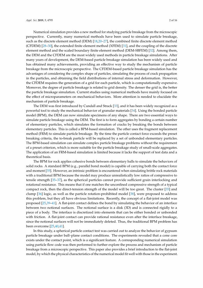
A typical flat-joint contact can be represented by the model shown in Figure 7. A flat-jointed material consists of rigid balls joined by flat-joint contacts. The effective surface of each ball is defined by the notional surfaces of its pieces, which interact at each flat-joint contact with the notional surface of the contact piece. Balls in a flat-jointed material are depicted as spherical cores and several skirted faces, which can provide resistance to rotation even after bond breaking. The skirted faces are deleted when the relative displacement at a flat-joint contact becomes greater than the flat-joint diameter. If the two balls are in contact again, the behavior will be that of between spherical surfaces. The interface between notional surfaces is a line (in 2D) or a disk (in 3D) and discretized into a number of elements in both circumferential and radial directions. Since the destruction of each element is relatively independent, partial damage of a contact can be achieved.

Figure 6. Morphologies after breakage: (a) contact point; (b) cone area; and (c) cone core.

3. Numerical Simulation

The particle-contact test for gypsum was simulated by the three-dimensional particle flow code(PFC3D) (Itasca Consulting Group, Inc. Minneapolis, MN, USA), which was developed by Itasca and awidely used the DEM software program. The material-modeling support of the PFC was used forgenerating the specimen and for performing standard rock tests.

The numerical model in the PFC is composed of rigid balls that interact at their contacts. The PFCmodel was originally developed to simulate the micromechanical behavior of noncohesive mediasuch as soils and sands [33]. In addition, the built-in bonded-particle model (BPM) for rock appliescohesive bonds between elementary balls to simulate the behaviors of solid rocks [35], in which crackformation is simulated through the breaking of bonds, while fracture propagation is obtained by thecoalescence of multiple bond breakages. In this study, we bound uncrushable elementary balls togetherto represent specimens that can be crushed when the external force exceeds their strength.

3.1. Flat-Joint Model

A typical flat-joint contact can be represented by the model shown in Figure 7. A flat-jointedmaterial consists of rigid balls joined by flat-joint contacts. The effective surface of each ball is definedby the notional surfaces of its pieces, which interact at each flat-joint contact with the notional surface ofthe contact piece. Balls in a flat-jointed material are depicted as spherical cores and several skirted faces,which can provide resistance to rotation even after bond breaking. The skirted faces are deleted whenthe relative displacement at a flat-joint contact becomes greater than the flat-joint diameter. If the twoballs are in contact again, the behavior will be that of between spherical surfaces. The interface betweennotional surfaces is a line (in 2D) or a disk (in 3D) and discretized into a number of elements in bothcircumferential and radial directions. Since the destruction of each element is relatively independent,partial damage of a contact can be achieved.

Each element can be either bonded or unbonded, and the breakage of each element contributespartial damage to the interface. The behavior of a bonded element is linearly elastic, and the bondbreaks when the strength limit is exceeded. The behavior of an unbonded element is linearly elasticand frictional, and the shear strength meets the Coulomb criterion. A tensile load is carried only in abonded region. The force–displacement response of the flat-joint interface includes evolving from afully bonded state to a frictional state.

Appl. Sci. 2019, 9, 4795 7 of 16Appl. Sci. 2019, 9, x FOR PEER REVIEW 7 of 16

Figure 7. A typical flat-joint contact

Each element can be either bonded or unbonded, and the breakage of each element contributes partial damage to the interface. The behavior of a bonded element is linearly elastic, and the bond breaks when the strength limit is exceeded. The behavior of an unbonded element is linearly elastic and frictional, and the shear strength meets the Coulomb criterion. A tensile load is carried only in a bonded region. The force–displacement response of the flat-joint interface includes evolving from a fully bonded state to a frictional state.

3.2. Model Calibration and Validation

To simulate the macroscopic phenomena of the experimental test in numerical modeling, repeated calculation and adjustment were required for model calibration. The numerical model was constructed and calibrated against the experimental results. In this paper, parameter adjusting methods were referred to the PFC official handbook. Studies have shown that the size of elementary particles has a certain effect on the mechanical properties of the numerical model [43,44]. When the elementary particle size is too large, the macroscopic mechanical properties of the model are unstable. The macroscopic mechanical properties of the model are not affected when the size of the elementary particle is sufficiently small. When the elementary particle size is too small, the number of particles in a numerical model will greatly increase to a point where the computational complexity will be unacceptable. We set the minimum diameter of elementary particles to 1.0 mm and the ratio of maximum to minimum size to 1.6. The ratio of model diameter to median particle size (𝐿/𝑑) is 38.5, and the effect on the simulation is very small, according to Ding [45].

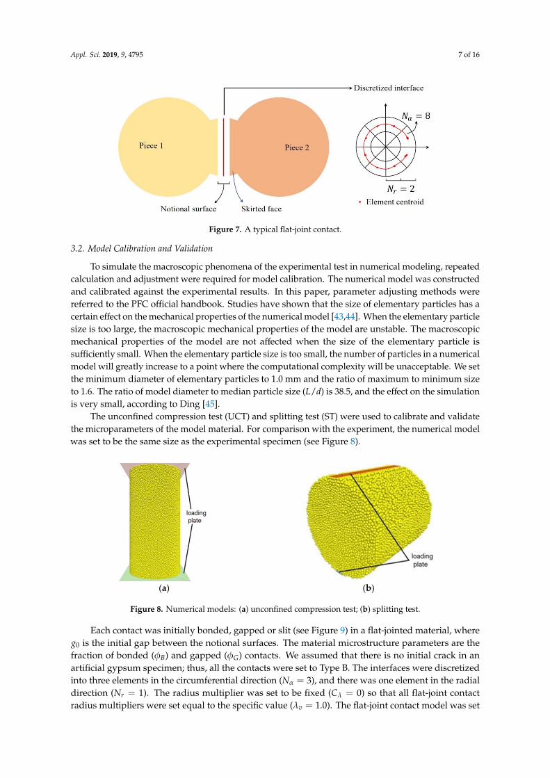
The unconfined compression test (UCT) and splitting test (ST) were used to calibrate and validate the microparameters of the model material. For comparison with the experiment, the numerical model was set to be the same size as the experimental specimen (see Figure 8).

(a)

(b)

Figure 8. Numerical models: (a) unconfined compression test; (b) splitting test.

Each contact was initially bonded, gapped or slit (see Figure 9) in a flat-jointed material, where 𝑔 is the initial gap between the notional surfaces. The material microstructure parameters are the

Figure 7. A typical flat-joint contact.

3.2. Model Calibration and Validation

To simulate the macroscopic phenomena of the experimental test in numerical modeling, repeatedcalculation and adjustment were required for model calibration. The numerical model was constructedand calibrated against the experimental results. In this paper, parameter adjusting methods werereferred to the PFC official handbook. Studies have shown that the size of elementary particles has acertain effect on the mechanical properties of the numerical model [43,44]. When the elementary particlesize is too large, the macroscopic mechanical properties of the model are unstable. The macroscopicmechanical properties of the model are not affected when the size of the elementary particle issufficiently small. When the elementary particle size is too small, the number of particles in a numericalmodel will greatly increase to a point where the computational complexity will be unacceptable. We setthe minimum diameter of elementary particles to 1.0 mm and the ratio of maximum to minimum sizeto 1.6. The ratio of model diameter to median particle size (L/d) is 38.5, and the effect on the simulationis very small, according to Ding [45].

The unconfined compression test (UCT) and splitting test (ST) were used to calibrate and validatethe microparameters of the model material. For comparison with the experiment, the numerical modelwas set to be the same size as the experimental specimen (see Figure 8).

Appl. Sci. 2019, 9, x FOR PEER REVIEW 7 of 16

Figure 7. A typical flat-joint contact

Each element can be either bonded or unbonded, and the breakage of each element contributes partial damage to the interface. The behavior of a bonded element is linearly elastic, and the bond breaks when the strength limit is exceeded. The behavior of an unbonded element is linearly elastic and frictional, and the shear strength meets the Coulomb criterion. A tensile load is carried only in a bonded region. The force–displacement response of the flat-joint interface includes evolving from a fully bonded state to a frictional state.

3.2. Model Calibration and Validation

To simulate the macroscopic phenomena of the experimental test in numerical modeling, repeated calculation and adjustment were required for model calibration. The numerical model was constructed and calibrated against the experimental results. In this paper, parameter adjusting methods were referred to the PFC official handbook. Studies have shown that the size of elementary particles has a certain effect on the mechanical properties of the numerical model [43,44]. When the elementary particle size is too large, the macroscopic mechanical properties of the model are unstable. The macroscopic mechanical properties of the model are not affected when the size of the elementary particle is sufficiently small. When the elementary particle size is too small, the number of particles in a numerical model will greatly increase to a point where the computational complexity will be unacceptable. We set the minimum diameter of elementary particles to 1.0 mm and the ratio of maximum to minimum size to 1.6. The ratio of model diameter to median particle size (𝐿/𝑑) is 38.5, and the effect on the simulation is very small, according to Ding [45].

The unconfined compression test (UCT) and splitting test (ST) were used to calibrate and validate the microparameters of the model material. For comparison with the experiment, the numerical model was set to be the same size as the experimental specimen (see Figure 8).

(a)

(b)

Figure 8. Numerical models: (a) unconfined compression test; (b) splitting test.

Each contact was initially bonded, gapped or slit (see Figure 9) in a flat-jointed material, where 𝑔 is the initial gap between the notional surfaces. The material microstructure parameters are the

Figure 8. Numerical models: (a) unconfined compression test; (b) splitting test.

Each contact was initially bonded, gapped or slit (see Figure 9) in a flat-jointed material, whereg0 is the initial gap between the notional surfaces. The material microstructure parameters are thefraction of bonded (φB) and gapped (φG) contacts. We assumed that there is no initial crack in anartificial gypsum specimen; thus, all the contacts were set to Type B. The interfaces were discretizedinto three elements in the circumferential direction (Nα = 3), and there was one element in the radialdirection (Nr = 1). The radius multiplier was set to be fixed (Cλ = 0) so that all flat-joint contactradius multipliers were set equal to the specific value (λv = 1.0). The flat-joint contact model was set

Appl. Sci. 2019, 9, 4795 8 of 16

to be installed at all ball–ball contacts with a gap less than or equal to 0.0002 m (gi = 2.0 × 10−4 m).The porosity-considered bulk density was set to 2650 kg/m3. The above parameters were fixed duringthe calibration process.

Appl. Sci. 2019, 9, x FOR PEER REVIEW 8 of 16

fraction of bonded (𝜙 ) and gapped (𝜙 ) contacts. We assumed that there is no initial crack in an artificial gypsum specimen; thus, all the contacts were set to Type B. The interfaces were discretized into three elements in the circumferential direction (𝑁 3), and there was one element in the radial direction (𝑁 1). The radius multiplier was set to be fixed (𝐶 0) so that all flat-joint contact radius multipliers were set equal to the specific value (𝜆 1.0). The flat-joint contact model was set to be installed at all ball–ball contacts with a gap less than or equal to 0.0002 m (𝑔 2.0 × 10 m). The porosity-considered bulk density was set to 2650 kg/m . The above parameters were fixed during the calibration process.

Figure 9. Initial microstructure of flat-joint contact

The calibration process involves the trial-and-error adjustment of the following micromechanical parameters: effective modulus 𝐸∗ (flat joint) and 𝐸∗ (linear), normal-to-shear stiffness ratio 𝜅∗ (flat joint) and 𝜅∗ (linear), friction coefficient 𝜇 (flat joint) and 𝜇 (linear), tensile strength 𝜎 , cohesion 𝑐, and friction angle 𝜙. All the tested values of these micromechanical parameters are listed in Table 2, and the calibration work was conducted using orthogonal experimental design. Note that in this study, 𝐸 ∗= 𝐸∗ , 𝜅∗ = 𝜅∗ , and 𝜇 = 𝜇 .

Table 2. Tested values of micromechanical parameters

Parameters Value 𝐸∗ (GPa) 6.0, 8.0, 12.0 𝜅∗ 2.0, 2.5, 3.0 𝜇 0.3, 0.5, 0.8 𝜎 (MPa) 3.0, 5.0, 8.0 𝑐 (MPa) 20.0, 30.0, 60.0 𝜙 (°) 25.0, 30.0, 35.0

The normal and shear stiffnesses were set based on a specified deformability by defining the effective modulus (𝐸∗) and normal to shear stiffness ratio (𝜅∗): 𝑘 𝐸∗𝐿 , 𝑘 𝑘𝜅∗ with 𝐿 𝑅 𝑅 , ball ball𝑅 , ball facet (1)

The macroproperties used for model calibration include unconfined compressive strength, tensile strength, elastic modulus, and Poisson’s ratio. The model sensitivity to key micromechanical parameters was analyzed with a multifactor Analysis of Variance (ANOVA) at 5% significance level (𝛼 0.05). The F values and associated p-values are shown in Figure 10. We can accept the hypothesis that the property is sensitive to the factor if the corresponding p-value is less than 𝛼; otherwise, the property and the factor are relatively independent variates.

Figure 9. Initial microstructure of flat-joint contact.

The calibration process involves the trial-and-error adjustment of the following micromechanicalparameters: effective modulus E∗ (flat joint) and E∗lnm (linear), normal-to-shear stiffness ratio κ∗ (flatjoint) and κ∗lnm (linear), friction coefficient µ (flat joint) and µlnm (linear), tensile strength σc, cohesion c,and friction angle φ. All the tested values of these micromechanical parameters are listed in Table 2,and the calibration work was conducted using orthogonal experimental design. Note that in this study,E∗= E∗lnm, κ∗ = κ∗lnm, and µ = µlnm.

Table 2. Tested values of micromechanical parameters.

Parameters Value

E∗ (GPa) 6.0, 8.0, 12.0κ∗ 2.0, 2.5, 3.0µ 0.3, 0.5, 0.8

σc (MPa) 3.0, 5.0, 8.0c (MPa) 20.0, 30.0, 60.0φ (◦) 25.0, 30.0, 35.0

The normal and shear stiffnesses were set based on a specified deformability by defining theeffective modulus (E∗) and normal to shear stiffness ratio (κ∗):

kn =E∗

L, ks =

kn

κ∗with L =

{R(1) + R(2), ball− ballR(1), ball− facet

(1)

The macroproperties used for model calibration include unconfined compressive strength, tensilestrength, elastic modulus, and Poisson’s ratio. The model sensitivity to key micromechanical parameterswas analyzed with a multifactor Analysis of Variance (ANOVA) at 5% significance level (α = 0.05).The F values and associated p-values are shown in Figure 10. We can accept the hypothesis that theproperty is sensitive to the factor if the corresponding p-value is less than α; otherwise, the propertyand the factor are relatively independent variates.

The following correlations are evident in Figure 10:

1. The unconfined compressive strength is sensitive to σc, as well as c and φ;2. The tensile strength is highly sensitive to σc and can be affected by κ∗;3. The elastic modulus is highly sensitive to E∗ and κ∗;4. Poisson’s ratio is sensitive to κ∗ and will be affected by c and φ.

During the model calibration process, some tests were applied with different random seeds tocheck the model’s reliability. The results showed that the calculated coefficients of variation for thesimulated macroproperties were less than 1%.

The above observations indicate certain correlations between the micromechanical parametersand macroproperties. However, this paper does not intend to establish a quantitative prediction modelof the macroproperties of flat-jointed material. The parametric study was primarily conducted to

Appl. Sci. 2019, 9, 4795 9 of 16

optimize the calibration process. A set of best-fit parameters were obtained based on the parametricstudy, as listed in Table 3. Note that in this study, E∗ = E∗lnm, κ∗ = κ∗lnm, and µ = µlnm.Appl. Sci. 2019, 9, x FOR PEER REVIEW 9 of 16

p=0.546

p=0.626

p=0.573

p=0.000

p=0.000

p=0.000

E*

κ*

μ

σc

c

φ

0 50 100 150 200 250 300 350

F value (a)

p=0.671

p=0.012

p=0.737

p=0.000

p=0.772

p=0.899

E*

κ*

μ

σc

c

φ

0 500 1000 1500 2000 2500

F value (b)

p=0.000

p=0.000

p=0.832

p=0.902

p=0.365

p=0.210

E*

κ*

μ

σc

c

φ

0 500 1000 1500 2000 2500

F value (c)

p=0.923

p=0.000

p=0.568

p=0.861

p=0.008

p=0.009

E*

κ*

μ

σc

c

φ

0 20 40 60 80 100 120 140 160

F value (d)

Figure 10. Results of a multifactor ANOVA (α = 0.05): (a) unconfined compressive strength; (b) tensile strength; (c) elastic modulus; and (d) Poisson’s ratio.

The following correlations are evident in Figure 10: 1. The unconfined compressive strength is sensitive to 𝜎 , as well as 𝑐 and 𝜙; 2. The tensile strength is highly sensitive to 𝜎 and can be affected by 𝜅∗; 3. The elastic modulus is highly sensitive to 𝐸∗ and 𝜅∗; 4. Poisson’s ratio is sensitive to 𝜅∗ and will be affected by 𝑐 and 𝜙.

During the model calibration process, some tests were applied with different random seeds to check the model’s reliability. The results showed that the calculated coefficients of variation for the simulated macroproperties were less than 1%.

The above observations indicate certain correlations between the micromechanical parameters and macroproperties. However, this paper does not intend to establish a quantitative prediction model of the macroproperties of flat-jointed material. The parametric study was primarily conducted to optimize the calibration process. A set of best-fit parameters were obtained based on the parametric study, as listed in Table 3. Note that in this study, 𝐸∗ = 𝐸∗ , 𝜅∗ = 𝜅∗ , and 𝜇 = 𝜇 .

Table 3. Tested values of micromechanical parameters

Parameters Value 𝜌 (kg/m ) 2650 𝑁 1 𝑁 3 𝐶 0 𝜆 1 𝑔 (m) 2.0 × 10 𝜙 1.0 𝐸∗ (GPa) 8.0 𝜅∗ 3.0 𝜇 0.577 𝜎 (MPa) 4.0 𝑐 (MPa) 23.0

Figure 10. Results of a multifactor ANOVA (α = 0.05): (a) unconfined compressive strength; (b) tensilestrength; (c) elastic modulus; and (d) Poisson’s ratio.

Table 3. Tested values of micromechanical parameters.

Parameters Value

ρb (kg/m3) 2650Nr 1Nα 3Cλ 0λv 1

gi (m) 2.0 × 10−4

φB 1.0E∗ (GPa) 8.0κ∗ 3.0µ 0.577

σc (MPa) 4.0c (MPa) 23.0φ (◦) 30.0

The test results were compared with those of the experiments. The force–displacement curves areshown in Figure 11. The result for the experiment was the average curve of five repeated tests.

The displacement during the initial stage of the splitting test was relatively large. A possiblereason for this was that the contact area was relatively small and the steel bar used for loading maynot have been absolutely flat; it was difficult to ensure complete contact between a specimen and theloading equipment; thus, the initial stiffness was relatively small. However, the slope and peak valueof the numerical model corresponded with those of the experiment very well.

Appl. Sci. 2019, 9, 4795 10 of 16

Appl. Sci. 2019, 9, x FOR PEER REVIEW 10 of 16 𝜙 (°) 30.0

The test results were compared with those of the experiments. The force–displacement curves are shown in Figure 11. The result for the experiment was the average curve of five repeated tests.

(a)

(b)

Figure 11. Test results: (a) stress–strain curve for unconfined compression test; (b) force–displacement curve for splitting test.

The displacement during the initial stage of the splitting test was relatively large. A possible reason for this was that the contact area was relatively small and the steel bar used for loading may not have been absolutely flat; it was difficult to ensure complete contact between a specimen and the loading equipment; thus, the initial stiffness was relatively small. However, the slope and peak value of the numerical model corresponded with those of the experiment very well.

The results show that the numerical model was well fitted with the mechanical properties of high-strength gypsum we used and could reflect its basic mechanical characteristics. The microparameters were well calibrated and were suitable for the study of particle breakage under ball–plane contact conditions.

The physical characteristics for numerical material are shown in Table 4

Table 4. Physical characteristics for numerical model

Unconfined Compressive Strength

Elastic Modulus

Poisson's Ratio

Tensile Strength

Specific Gravity

40.97 MPa 7.58 GPa 0.29 2.87 MPa 2.65

The shape and size of the numerical model were consistent with the spherical gypsum particles in the experimental test. The diameter of the model was 50 mm. The minimum diameter of elementary particles was 1.0 mm, and the ratio of maximum to minimum size was 1.6. The ratio of model diameter to median particle size (𝐿/𝑑) was 38.5, and the effect on the simulation is generally very small, according to Ding [45].

The original model is shown in Figure 12. We used the wall unit in the PFC to simulate the contact surface and the loading plate. The loading speed of the numerical simulation was set in reference to that of the experiment. Note that the contact condition at the bottom was different from that of the experiment. According to Saint-Venant's Principle, the difference between the effects of different contact conditions at the bottom on the upper part of the specimen is very small. In this paper, only the morphology of the upper part is discussed to study the particle breakage under ball–plane contact conditions.

Figure 11. Test results: (a) stress–strain curve for unconfined compression test; (b) force–displacementcurve for splitting test.

The results show that the numerical model was well fitted with the mechanical properties ofhigh-strength gypsum we used and could reflect its basic mechanical characteristics. The microparameterswere well calibrated and were suitable for the study of particle breakage under ball–planecontact conditions.

The physical characteristics for numerical material are shown in Table 4

Table 4. Physical characteristics for numerical model.

UnconfinedCompressive Strength Elastic Modulus Poisson’s Ratio Tensile Strength Specific Gravity

40.97 MPa 7.58 GPa 0.29 2.87 MPa 2.65

The shape and size of the numerical model were consistent with the spherical gypsum particles inthe experimental test. The diameter of the model was 50 mm. The minimum diameter of elementaryparticles was 1.0 mm, and the ratio of maximum to minimum size was 1.6. The ratio of model diameterto median particle size (L/d) was 38.5, and the effect on the simulation is generally very small, accordingto Ding [45].

The original model is shown in Figure 12. We used the wall unit in the PFC to simulate thecontact surface and the loading plate. The loading speed of the numerical simulation was set inreference to that of the experiment. Note that the contact condition at the bottom was different fromthat of the experiment. According to Saint-Venant’s Principle, the difference between the effects ofdifferent contact conditions at the bottom on the upper part of the specimen is very small. In this paper,only the morphology of the upper part is discussed to study the particle breakage under ball–planecontact conditions.

We also used the built-in FISH functions in the PFC to enable fragment visualization by paintingbroken contacts with different colors, which made it possible to observe the particle breakage behavior.

Appl. Sci. 2019, 9, 4795 11 of 16Appl. Sci. 2019, 9, x FOR PEER REVIEW 11 of 16

Figure 12. Original numerical model

We also used the built-in FISH functions in the PFC to enable fragment visualization by painting broken contacts with different colors, which made it possible to observe the particle breakage behavior.

3.3. Results

In the numerical simulation, the wall units worked as loading planes and measured the displacement as well as the contact force. The main purpose of this paper is not to validate the statistical rules of maximum contact force, which has been the subject of many previous studies [22–24,26,27]. The DEM simulation was intended to determine the general mechanism of contact breakage under ball–plane conditions from a microscopic perspective.

3.3.1. Mechanical Characteristics

The force–displacement curve recorded by numerical simulation was compared with that of the experiments, as shown in Figure 13. The numerical model fit the force–displacement curve very well in the particle contact test. The maximum ball–plane contact force of the numerical model was 6.989 kN, and the equivalent stiffness was approximately 8.160 kN/mm. It can also be seen from the curve that the local breakage of the numerical result was not evident at the initial stage. The reason could be that the model was an aggregate of a finite number of rigid elementary particles, which limited the degree of fragmentation at a relatively small displacement. However, the advantage of this model on the simulation of particle contact was appreciable when it was compared with previous studies using a parallel-bond model [18], the result of which had an unrealistically large displacement.

Figure 12. Original numerical model.

3.3. Results

In the numerical simulation, the wall units worked as loading planes and measured thedisplacement as well as the contact force. The main purpose of this paper is not to validate the statisticalrules of maximum contact force, which has been the subject of many previous studies [22–24,26,27].The DEM simulation was intended to determine the general mechanism of contact breakage underball–plane conditions from a microscopic perspective.

3.3.1. Mechanical Characteristics

The force–displacement curve recorded by numerical simulation was compared with that of theexperiments, as shown in Figure 13. The numerical model fit the force–displacement curve very well inthe particle contact test. The maximum ball–plane contact force of the numerical model was 6.989 kN,and the equivalent stiffness was approximately 8.160 kN/mm. It can also be seen from the curve thatthe local breakage of the numerical result was not evident at the initial stage. The reason could bethat the model was an aggregate of a finite number of rigid elementary particles, which limited thedegree of fragmentation at a relatively small displacement. However, the advantage of this model onthe simulation of particle contact was appreciable when it was compared with previous studies using aparallel-bond model [18], the result of which had an unrealistically large displacement.

Appl. Sci. 2019, 9, x FOR PEER REVIEW 11 of 16

Figure 12. Original numerical model

We also used the built-in FISH functions in the PFC to enable fragment visualization by painting broken contacts with different colors, which made it possible to observe the particle breakage behavior.

3.3. Results

In the numerical simulation, the wall units worked as loading planes and measured the displacement as well as the contact force. The main purpose of this paper is not to validate the statistical rules of maximum contact force, which has been the subject of many previous studies [22–24,26,27]. The DEM simulation was intended to determine the general mechanism of contact breakage under ball–plane conditions from a microscopic perspective.

3.3.1. Mechanical Characteristics

The force–displacement curve recorded by numerical simulation was compared with that of the experiments, as shown in Figure 13. The numerical model fit the force–displacement curve very well in the particle contact test. The maximum ball–plane contact force of the numerical model was 6.989 kN, and the equivalent stiffness was approximately 8.160 kN/mm. It can also be seen from the curve that the local breakage of the numerical result was not evident at the initial stage. The reason could be that the model was an aggregate of a finite number of rigid elementary particles, which limited the degree of fragmentation at a relatively small displacement. However, the advantage of this model on the simulation of particle contact was appreciable when it was compared with previous studies using a parallel-bond model [18], the result of which had an unrealistically large displacement.

Figure 13. Force–displacement curve in numerical simulation.

Appl. Sci. 2019, 9, 4795 12 of 16

3.3.2. Breakage Behavior

In the numerical test, the breakage phenomenon of the specimen was consistent with theexperimental result. First, local breakage was produced, and a small platform was formed at thecontact point. Then, the stage for crack nucleation and crack propagation followed. Finally, the contactforce exceeded its strength, and the specimen broke into two pieces.

By means of numerical simulation, we could observe the law of morphological changes insidethe specimen as well as the specific form of failure. The top view of the overall breakage shows thedestruction form and the cracks in the surface layer of the specimen (see Figure 14a). The elementaryparticles and failed bonds are shown in the figure. The tensile and shear failure of bonds are indicatedby arrows and texts (see Figure 14b and Figure 16c).

Appl. Sci. 2019, 9, x FOR PEER REVIEW 12 of 16

Figure 13. Force–displacement curve in numerical simulation

3.3.2. Breakage Behavior

In the numerical test, the breakage phenomenon of the specimen was consistent with the experimental result. First, local breakage was produced, and a small platform was formed at the contact point. Then, the stage for crack nucleation and crack propagation followed. Finally, the contact force exceeded its strength, and the specimen broke into two pieces.

By means of numerical simulation, we could observe the law of morphological changes inside the specimen as well as the specific form of failure. The top view of the overall breakage shows the destruction form and the cracks in the surface layer of the specimen (see Figure 14a). The elementary particles and failed bonds are shown in the figure. The tensile and shear failure of bonds are indicated by arrows and texts (see Figure 14b and 16c).

(a)

(b)

(c)

Figure 14. Morphologies after breakage: (a) overall breakage (top view); (b) partial enlargement (A-A); and (c) partial enlargement (B-B).

The result indicates that most of the broken contacts failed in tension, which was consistent with the theoretical expectations [46]. It is noteworthy that there was a circular area under the loading plane with a significantly smaller number of cracks, which was similar to the result of the experiment (see Figure 6a). Figure 14b and 16c show enlarged images of the cone core after the overall breakage to study the micromechanical process and mechanism underlying the cone core formation. The small images shown in Figure 14 and 16 are zoomed sections of Figure 14a. The transparency of elementary particles was set to 60%, and only particles and cracks in a limited area in front of the cross-section can be observed.

It is clear in Figure 14b and 16c that most of the bonded contacts in the area under the loading plane did not break after the overall breakage. The image acquired from the cross-section perpendicular to the fracture plane also indicates that the shape of the unbroken area was similar to a cone. Another important feature is that shear failures of bonds could be found at the edge of the cone core. This indicates that there was a relative movement trend between the cone core and the rest of the specimen. Figure 15 shows the velocity of the elementary particles in Figure 14c. The arrow is located in the center of the particle pointing to the direction of the velocity, and the length of the arrow is linearly related to the velocity of the particle. It is clear that particles in the blue region basically moved downward as a whole.

Figure 14. Morphologies after breakage: (a) overall breakage (top view); (b) partial enlargement (A-A);and (c) partial enlargement (B-B).

The result indicates that most of the broken contacts failed in tension, which was consistent withthe theoretical expectations [46]. It is noteworthy that there was a circular area under the loading planewith a significantly smaller number of cracks, which was similar to the result of the experiment (seeFigure 6a). Figure 14b and Figure 16c show enlarged images of the cone core after the overall breakageto study the micromechanical process and mechanism underlying the cone core formation. The smallimages shown in Figure 14 and Figure 16 are zoomed sections of Figure 14a. The transparency ofelementary particles was set to 60%, and only particles and cracks in a limited area in front of thecross-section can be observed.

It is clear in Figure 14b and Figure 16c that most of the bonded contacts in the area under theloading plane did not break after the overall breakage. The image acquired from the cross-sectionperpendicular to the fracture plane also indicates that the shape of the unbroken area was similar to acone. Another important feature is that shear failures of bonds could be found at the edge of the conecore. This indicates that there was a relative movement trend between the cone core and the rest ofthe specimen. Figure 15 shows the velocity of the elementary particles in Figure 14c. The arrow islocated in the center of the particle pointing to the direction of the velocity, and the length of the arrowis linearly related to the velocity of the particle. It is clear that particles in the blue region basicallymoved downward as a whole.

Appl. Sci. 2019, 9, 4795 13 of 16Appl. Sci. 2019, 9, x FOR PEER REVIEW 13 of 16

Figure 15. Force–displacement curve in numerical simulation

The bond states at different loading stages are shown in Figure 16. The elementary particles and tensile failures on the cross-section B-B in Figure 14a are displayed. All shear failures are shown. The results show that local breakages first occurred at the surface and inside the specimen under the loading plate; most of the cracks exhibited tensile failure, while some cracks in the annular area centered around the loading point exhibited shear failure (see Figure 16a). Since the load continued to increase, shear cracks developed to the inner of the specimen and eventually formed a cone core (see Figure 16b and 18c). The cone core moved downward under the loading plate and ultimately split the specimen into pieces.

Figure 16. Bond state at different loading stages: (a) 2.0157 kN; (b) 4.0892 kN; and (c) 6.1862 kN.

4. Discussion

Through the experiment, the contact breakage behavior of gypsum particles was analyzed. The force–displacement curve was almost linear, and the breakage was an instantaneous brittle fracture. A significant feature of particle contact breakage was the observation of a cone core formed at the contact point. Limited by the experimental conditions, the formation process and mechanism of the cone core could not be observed by conventional means.

Figure 15. Force–displacement curve in numerical simulation.

The bond states at different loading stages are shown in Figure 16. The elementary particlesand tensile failures on the cross-section B-B in Figure 14a are displayed. All shear failures are shown.The results show that local breakages first occurred at the surface and inside the specimen underthe loading plate; most of the cracks exhibited tensile failure, while some cracks in the annular areacentered around the loading point exhibited shear failure (see Figure 16a). Since the load continued toincrease, shear cracks developed to the inner of the specimen and eventually formed a cone core (seeFigure 16b and 18c). The cone core moved downward under the loading plate and ultimately split thespecimen into pieces.

Appl. Sci. 2019, 9, x FOR PEER REVIEW 13 of 16

Figure 15. Force–displacement curve in numerical simulation

The bond states at different loading stages are shown in Figure 16. The elementary particles and tensile failures on the cross-section B-B in Figure 14a are displayed. All shear failures are shown. The results show that local breakages first occurred at the surface and inside the specimen under the loading plate; most of the cracks exhibited tensile failure, while some cracks in the annular area centered around the loading point exhibited shear failure (see Figure 16a). Since the load continued to increase, shear cracks developed to the inner of the specimen and eventually formed a cone core (see Figure 16b and 18c). The cone core moved downward under the loading plate and ultimately split the specimen into pieces.

Figure 16. Bond state at different loading stages: (a) 2.0157 kN; (b) 4.0892 kN; and (c) 6.1862 kN.

4. Discussion

Through the experiment, the contact breakage behavior of gypsum particles was analyzed. The force–displacement curve was almost linear, and the breakage was an instantaneous brittle fracture. A significant feature of particle contact breakage was the observation of a cone core formed at the contact point. Limited by the experimental conditions, the formation process and mechanism of the cone core could not be observed by conventional means.

Figure 16. Bond state at different loading stages: (a) 2.0157 kN; (b) 4.0892 kN; and (c) 6.1862 kN.

4. Discussion

Through the experiment, the contact breakage behavior of gypsum particles was analyzed.The force–displacement curve was almost linear, and the breakage was an instantaneous brittle fracture.A significant feature of particle contact breakage was the observation of a cone core formed at thecontact point. Limited by the experimental conditions, the formation process and mechanism of thecone core could not be observed by conventional means.

The results of the numerical simulation now provide evidence for the mechanism of the formationof cone cores. The process of contact breakage for gypsum particles under ball–plane contact conditionscan be described as follows:

Appl. Sci. 2019, 9, 4795 14 of 16

Due to the stress concentration, local breakage occurred at the point where the specimen was incontact with the loading plate (see Figure 17b). The breaking part of the specimen was confined by theconstraint of the surrounding specimen and was gradually compressed into the specimen during theloading process. The breaking part pressed into the inner part continually compressed the surroundingspecimen. The shear cracks developed inside the specimen and gradually formed a conical region (seeFigure 17c). The cone core was continuously squeezed downwards into the specimen, and a tensileforce perpendicular to the loading direction was exerted on the specimen inside. When the tensilestress inside the specimen exceeded its strength, the fracture formed and rapidly expanded. Finally,overall breakage occurred (see Figure 17d).

Appl. Sci. 2019, 9, x FOR PEER REVIEW 14 of 16

The results of the numerical simulation now provide evidence for the mechanism of the formation of cone cores. The process of contact breakage for gypsum particles under ball–plane contact conditions can be described as follows:

Due to the stress concentration, local breakage occurred at the point where the specimen was in contact with the loading plate (see Figure 17b). The breaking part of the specimen was confined by the constraint of the surrounding specimen and was gradually compressed into the specimen during the loading process. The breaking part pressed into the inner part continually compressed the surrounding specimen. The shear cracks developed inside the specimen and gradually formed a conical region (see Figure 17c). The cone core was continuously squeezed downwards into the specimen, and a tensile force perpendicular to the loading direction was exerted on the specimen inside. When the tensile stress inside the specimen exceeded its strength, the fracture formed and rapidly expanded. Finally, overall breakage occurred (see Figure 17d).

(a)

(b)

(c)

(d)

Figure 17. Breaking process under ball–plane contact condition: (a) original state; (b) local breakage; (c) formation of cone core; (d) particle breakage.

During the testing process, the position of the final fracture is affected by the original cracks or defects existing in the specimen. Under the action of tensile stress, a fracture forms at the place with the lowest strength.

Since the total number of elementary particles is limited, the simulation of local breakage is still not sufficiently precise. However, the trade-off is acceptable given the huge amount of computation. In future work, we will generalize this model to other brittle rock materials to further investigate the mechanism of particle breakage.

5. Conclusions

In this paper, the mechanism of spherical gypsum particle breakage under ball–plane contact condition was experimentally and numerically studied.

Particle contact tests of high-strength gypsum were carried out to investigate the characteristics of particle contact breakage under ball–plane conditions. Unconfined compression tests and splitting tests were performed to determine the physical parameters of the test material. The corresponding numerical simulation was performed using the DEM to study particle contact breakage in a microscopic way. The numerical specimen adopted a flat-joint model to simulate gypsum material. The validity of the methodology was verified by modeling the unconfined compression test and splitting test. The numerical model fitted with the results of the standard rock tests in several aspects, and this feature was also observed during the modeling of the particle contact test.

The conclusions are: (1) The particle breakage a under ball–plane contact condition was an instantaneous brittle

fracture. A cone core could be found under the contact area after breakage. (2) The flat-joint model in PFC is suitable for simulating brittle rock material, such that the results

of simulation were well fitted with the results of the experiment. By means of numerical simulation, the mechanism of particle contact breakage was observed from a micromechanics angle.

Figure 17. Breaking process under ball–plane contact condition: (a) original state; (b) local breakage;(c) formation of cone core; (d) particle breakage.

During the testing process, the position of the final fracture is affected by the original cracks ordefects existing in the specimen. Under the action of tensile stress, a fracture forms at the place withthe lowest strength.

Since the total number of elementary particles is limited, the simulation of local breakage is stillnot sufficiently precise. However, the trade-off is acceptable given the huge amount of computation.In future work, we will generalize this model to other brittle rock materials to further investigate themechanism of particle breakage.

5. Conclusions

In this paper, the mechanism of spherical gypsum particle breakage under ball–plane contactcondition was experimentally and numerically studied.

Particle contact tests of high-strength gypsum were carried out to investigate the characteristics ofparticle contact breakage under ball–plane conditions. Unconfined compression tests and splittingtests were performed to determine the physical parameters of the test material. The correspondingnumerical simulation was performed using the DEM to study particle contact breakage in a microscopicway. The numerical specimen adopted a flat-joint model to simulate gypsum material. The validity ofthe methodology was verified by modeling the unconfined compression test and splitting test. Thenumerical model fitted with the results of the standard rock tests in several aspects, and this featurewas also observed during the modeling of the particle contact test.

The conclusions are:

(1) The particle breakage a under ball–plane contact condition was an instantaneous brittle fracture.A cone core could be found under the contact area after breakage.

(2) The flat-joint model in PFC is suitable for simulating brittle rock material, such that the results ofsimulation were well fitted with the results of the experiment. By means of numerical simulation,the mechanism of particle contact breakage was observed from a micromechanics angle.

(3) During the loading process, the cone core would be formed by shear cracks under the contactregion. The tensile stress caused by the loading force and by the penetration of the cone corewould finally exceeds its strength, that the overall breakage occurs.

Appl. Sci. 2019, 9, 4795 15 of 16

Author Contributions: Conceptualization, J.Z. and S.Y.; formal analysis, S.Y., M.J. and J.Z.; software, S.Y., L.L.and C.Z.; writing—original draft, S.Y.; writing—review & editing, M.J., C.Z. and L.L.

Funding: This research was funded by National Natural Science Foundation of China (No. 51479138, No. 40972214).

Conflicts of Interest: The authors declare no conflict of interest. The funders had no role in the design of thestudy; in the collection, analyses, or interpretation of data; in the writing of the manuscript, or in the decision topublish the results.

References

1. Fukumoto, T. Particle breakage characteristics of granular soils. Soils Found. 1992, 32, 26–40. [CrossRef]2. Cavarretta, I.; Coop, M.R.; Osullivan, C. The influence of particle characteristics on the behaviour of coarse

grained soils. Geotechnique 2010, 60, 413–423. [CrossRef]3. Lee, I.K.; Coop, M.R. The intrinsic behaviour of a decomposed granite soil. Geotechnique 1995, 45, 117–130.

[CrossRef]4. Jiang, M.; Bai, R.; Liu, J.; Zhou, Y. Experimental study of inter-granular particles bonding behaviors for rock

microstructure. Chin. J. Rock Mech. Eng. 2013, 32, 1121–1128.5. Coop, M.; Lee, I. The behaviour of granular soils at elevated stresses. Predict. Soil Mech. 1993, 1992, 186–198.6. Luzzani, L.; MR, C. On the relationship between particle breakage and the critical state of sands. Soils Found.

2002, 42, 71–82. [CrossRef]7. Ueng, T.S.; Chen, T.J. Energy aspects of particle breakage in drained shear of sands. Geotechnique 2000, 50,

65–72. [CrossRef]8. Marsal, R.J. Large-scale testing of rockfill materials. J. Soil Mech. Found. Div. 1967, 93, 27–43.9. Hardin, B.O. Crushing of Soil Particles. J. Geotech. Eng. 1985, 111, 1177–1192. [CrossRef]10. Yokura, K.; Yamamoto, H.; Wu, Y. Crushing tests of soil particles by high pressure true tri-axial compression

apparatus. Jpn. Geotech. Soc. Spec. Publ. 2015, 1, 51–56. [CrossRef]11. Coop, M.; Sorensen, K.; Bodas Freitas, T.; Georgoutsos, G. Particle breakage during shearing of a carbonate

sand. Géotechnique 2004, 54, 157–163. [CrossRef]12. Xu, W.J.; Hu, R.L.; Tan, R.J. Some geomechanical properties of soil–rock mixtures in the Hutiao Gorge area,

China. Geotechnique 2007, 57, 255–264. [CrossRef]13. Liu, X.R.; Yi-Liang, T.U.; Wang, P.; Zhong, Z.L.; Tang, W.B.; Li-Bing, D.U. Particle breakage of soil-rock

aggregate based on large-scale direct shear tests. Chin. J. Geotech. Eng. 2017, 39, 1425–1434.14. Al-Douri, R.H.; Poulos, H.G. Static and cyclic direct shear tests on carbonate sands. Geotech. Test. J. 1992, 15,

138–157.15. Nakao, T.; Fityus, S. Direct shear testing of a marginal material using a large shear box. Geotech. Test. J. 2008,

31, 393–403.16. Nakata, Y.; Kato, Y.; Hyodo, M.; HYDE, A.F.; Murata, H. One-dimensional compression behaviour of

uniformly graded sand related to single particle crushing strength. Soils Found. 2001, 41, 39–51. [CrossRef]17. Zhao, C.; Hou, R.; Zhou, J. Particle contact characteristics of coarse-grained soils under normal contact. Eur.

J. Environ. Civ. Eng. 2018, 22, s114–s129.18. Zhou, J.; Yu, S.; Zhang, J.; Zhao, C. The process and mechanism for the contact breakage of marble particles.

J. Harbin Inst. Technol. 2018, 50, 110–119.19. Wang, Z. A Study on Contact Behaviors and Microscopic Constitutive Relations of Coarse-Grained Soils; Tongji

University: Shanghai, China, 12 September 2013.20. Lobo-Guerrero, S.; Vallejo, L.E. Discrete element method analysis of railtrack ballast degradation during

cyclic loading. Granul. Matter 2006, 8, 195. [CrossRef]21. Cil, M.; Alshibli, K. 3D evolution of sand fracture under 1D compression. Géotechnique 2014, 64, 351.

[CrossRef]22. Shi, D.; Zheng, L.; Xue, J.; Sun, J. DEM modeling of particle breakage in silica sands under one-dimensional

compression. Acta Mech. Solida Sin. 2016, 29, 78–94. [CrossRef]23. Liu, Y.; Liu, H.; Mao, H. DEM investigation of the effect of intermediate principle stress on particle breakage

of granular materials. Comput. Geotech. 2017, 84, 58–67. [CrossRef]24. Zheng, W.; Tannant, D.D. Grain breakage criteria for discrete element models of sand crushing under

one-dimensional compression. Comput. Geotech. 2018, 95, 231–239. [CrossRef]

Appl. Sci. 2019, 9, 4795 16 of 16

25. Wang, B.; Martin, U.; Rapp, S. Discrete element modeling of the single-particle crushing test for ballast stones.Comput. Geotech. 2017, 88, 61–73. [CrossRef]

26. Xu, M.; Hong, J.; Song, E. DEM study on the effect of particle breakage on the macro-and micro-behavior ofrockfill sheared along different stress paths. Comput. Geotech. 2017, 89, 113–127. [CrossRef]

27. Manso, J.; Marcelino, J.; Caldeira, L. Crushing and oedometer compression of rockfill using DEM. Comput.Geotech. 2018, 101, 11–22. [CrossRef]

28. Kh, A.B.; Mirghasemi, A.; Mohammadi, S. Numerical simulation of particle breakage of angular particlesusing combined DEM and FEM. Powder Technol. 2011, 205, 15–29.

29. Ma, G.; Zhou, W.; Chang, X.L.; Chen, M.X. A hybrid approach for modeling of breakable granular materialsusing combined finite-discrete element method. Granul. Matter 2016, 18, 7. [CrossRef]

30. Ma, G.; Zhou, W.; Chang, X.L. Modeling the particle breakage of rockfill materials with the cohesive crackmodel. Comput. Geotech. 2014, 61, 132–143. [CrossRef]

31. Druckrey, A.M.; Alshibli, K.A. 3D finite element modeling of sand particle fracture based on in situ X-raysynchrotron imaging. Int. J. Numer. Anal. Methods Geomech. 2016, 40, 105–116. [CrossRef]

32. Luo, T.; Ooi, E.; Chan, A.; Fu, S. Modeling the particle breakage by using combined DEM and SBFEM. InProceedings of the International Conference on Discrete Element Methods, Dalian, China, 1–4 August 2016;pp. 281–288.

33. Cundall, P.A.; Strack, O.D. A discrete numerical model for granular assemblies. Geotechnique 1979, 29, 47–65.[CrossRef]

34. Qian, J.; You, Z.; Huang, M.; Gu, X. A micromechanics-based model for estimating localized failure witheffects of fabric anisotropy. Comput. Geotech. 2013, 50, 90–100. [CrossRef]

35. Potyondy, D.O.; Cundall, P. A bonded-particle model for rock. Int. J. Rock Mech. Min. Sci. 2004, 41, 1329–1364.[CrossRef]

36. Cho, N.A.; Martin, C.; Sego, D. A clumped particle model for rock. Int. J. Rock Mech. Min. Sci. 2007, 44,997–1010. [CrossRef]

37. Zhang, Q.; Zhu, H.; Zhang, L.; Ding, X. Effect of micro-parameters on the Hoek-Brown strength parameter mifor intact rock using particle flow modeling. In Proceedings of the 46th US Rock Mechanics/GeomechanicsSymposium, Chicago, IL, USA, 24–27 June 2012.

38. Jiang, M.; Yu, H.S.; Harris, D. A novel discrete model for granular material incorporating rolling resistance.Comput. Geotech. 2005, 32, 340–357. [CrossRef]

39. Potyondy, D.O. A flat-jointed bonded-particle material for hard rock. In Proceedings of the 46th US RockMechanics/Geomechanics Symposium, Chicago, IL, USA, 24–27 June 2012.

40. Potyondy, D.O. A Flat-Jointed Bonded-Particle Model for Rock. In Proceedings of the 52nd U.S. RockMechanics/Geomechanics Symposium, Seattle, WA, USA, 21 August 2018; p. 12.

41. Wu, S.; Xu, X. A study of three intrinsic problems of the classic discrete element method using flat-jointmodel. Rock Mech. Rock Eng. 2016, 49, 1813–1830. [CrossRef]

42. Yin, X.; Ge, X.; Li, C.; Wang, S. Influences of loading rates on mechanical behaviors of rock materials. Chin. J.Rock Mech. Eng. 2010, 29, 2610–2615.

43. Cundall, P.A. Formulation of a three-dimensional distinct element model—Part I. A scheme to detect andrepresent contacts in a system composed of many polyhedral blocks. Int. J. Rock Mech. Min.Sci. Geomech.Abstr. 1988, 25, 107–116. [CrossRef]

44. Alefeld, G.; Mayer, G. Interval analysis: Theory and applications. J. Comput. Appl. Math. 2000, 121, 421–464.[CrossRef]

45. Ding, X.; Zhang, L.; Zhu, H.; Zhang, Q. Effect of model scale and particle size distribution on PFC3Dsimulation results. Rock Mech. Rock Eng. 2014, 47, 2139–2156. [CrossRef]

46. Hiramatsu, Y.; Oka, Y. Determination of the tensile strength of rock by a compression test of an irregular testpiece. Int. J. Rock Mech. Min.Sci. Geomech. Abstr. 1966, 3, 89–90. [CrossRef]

© 2019 by the authors. Licensee MDPI, Basel, Switzerland. This article is an open accessarticle distributed under the terms and conditions of the Creative Commons Attribution(CC BY) license (http://creativecommons.org/licenses/by/4.0/).