77
Micro Review Day 1: Product Markets Theory of Choice Total Utility & Marginal Utility Market Behaviors MR=MC
| Date post: | 25-Dec-2015 |
| Category: |
Documents |
| Upload: | molly-hill |
| View: | 215 times |
| Download: | 0 times |

Micro Review Day 1: Product MarketsTheory of Choice
Total Utility & Marginal UtilityMarket Behaviors
MR=MC

Production= Converting inputs into output

AnalyzingProduction

WidgetProduction Simulation

Inputs and Outputs• To earn profit, firms must make products (output)• Inputs are the resources used to make outputs. • Input resources are also called FACTORS.
Marginal Product =Change in Total Product
Change in Inputs
• Marginal Product (MP)- the additional output generated by additional inputs (workers).
• Total Physical Product (TP)- total output or quantity produced
• Average Product (AP)- the output per unit of input
Average Product =Total Product
Units of Labor

Production Analysis• What happens to the Total Product as you hire
more workers?• What happens to marginal product as you hire
more workers?• Why does this happens?The Law of Diminishing Marginal Returns
As variable resources (workers) are added to fixed resources (machinery, tool, etc.), the additional output produced from each new worker will eventually fall.
Too many cooks in the kitchen!

Graphing Production

With your partner calculate MP and AP then discuss what the graphs for TP, MP, and AP look like.
Remember quantity of workers goes on the x-axis.# of Workers
(Input)Total Product(TP)
PIZZASMarginal
Product(MP)Average
Product(AP)
0 0
1 10
2 25
3 45
4 60
5 70
6 75
7 75
8 70

# of Workers(Input)
Total Product(TP) PIZZAS
Marginal Product(MP)
Average Product(AP)
0 0 - -
1 10 10
2 25 15
3 45 20
4 60 15
5 70 10
6 75 5
7 75 0
8 70 -5
With your partner calculate MP and AP then discuss what the graphs for TP, MP, and AP look like.
Remember quantity of workers goes on the x-axis.

# of Workers(Input)
Total Product(TP) PIZZAS
Marginal Product(MP)
Average Product(AP)
0 0 - -
1 10 10 10
2 25 15 12.5
3 45 20 15
4 60 15 15
5 70 10 14
6 75 5 12.5
7 75 0 10.71
8 70 -5 8.75
With your partner calculate MP and AP then discuss what the graphs for TP, MP, and AP look like.
Remember quantity of workers goes on the x-axis.
# of Workers(Input)
Total Product(TP) PIZZAS
Marginal Product(MP)
Average Product(AP)
0 0 - -
1 10 10 10
2 25 15 12.5
3 45 20 15
4 60 15 15
5 70 10 14
6 75 5 12.5
7 75 0 10.71
8 70 -5 8.75
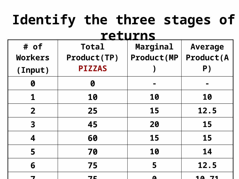
Identify the three stages of returns
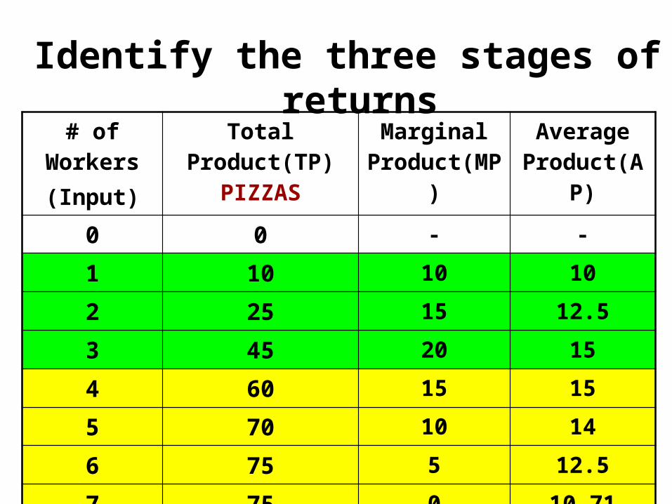
# of Workers(Input)
Total Product(TP) PIZZAS
Marginal Product(MP)
Average Product(AP)
0 0 - -
1 10 10 10
2 25 15 12.5
3 45 20 15
4 60 15 15
5 70 10 14
6 75 5 12.5
7 75 0 10.71
8 70 -5 8.75
Identify the three stages of returns

Three Stages of Returns
Total Product
Quantity of Labor
Marginal and
Average Product
Quantity of Labor
Total Product
Stage I: Increasing Marginal ReturnsMP rising. TP increasing at an increasing rate.
Why? Specialization.
Average Product
Marginal Product
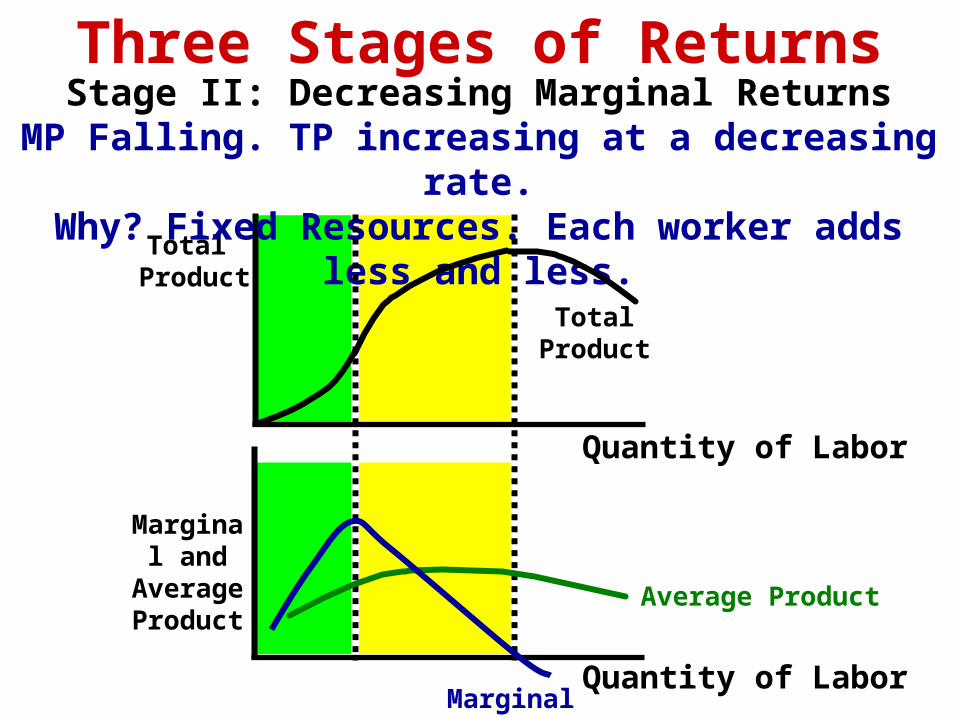
Three Stages of Returns
Total Product
Quantity of Labor
Marginal and
Average Product
Quantity of Labor
Total Product
Stage II: Decreasing Marginal ReturnsMP Falling. TP increasing at a decreasing rate.
Why? Fixed Resources. Each worker adds less and less.
Average Product
Marginal Product

Total Product
Quantity of Labor
Marginal and
Average Product
Quantity of Labor
Total Product
Stage III: Negative Marginal ReturnsMP is negative. TP decreasing. Workers get in each others way
Marginal Product
Average Product
Three Stages of Returns

More Examples of the Law of Diminishing Marginal Returns
Example #1: Learning curve when studying for an exam Fixed Resources-Amount of class time, textbook, etc.Variable Resources-Study time at homeMarginal return-
1st hour-large returns2nd hour-less returns3rd hour-small returns4th hour- negative returns (tired and confused)
Example #2: A Farmer has fixed resource of 8 acres planted of corn. If he doesn’t clear weeds he will get 30 bushels. If he clears weeds once he will get 50 bushels. Twice -57, Thrice-60. Additional returns diminishes each
time.
Costs of Production

Accountants vs. Economists
AccountingProfit
TotalRevenue
Accounting Costs(Explicit Only)
Accountants look at only EXPLICIT COSTS • Explicit costs (out of pocket costs) are payments
paid by firms for using the resources of others. • Example: Rent, Wages, Materials, Electricity Bills
Economists examine both the EXPLICIT COSTS and the IMPLICIT COSTS• Implicit costs are the opportunity costs that firms
“pay” for using their own resources• Example: Forgone Wage, Forgone Rent, Time
Economic Profit
TotalRevenue
Economic Costs (Explicit + Implicit)

Short-Run Production Costs
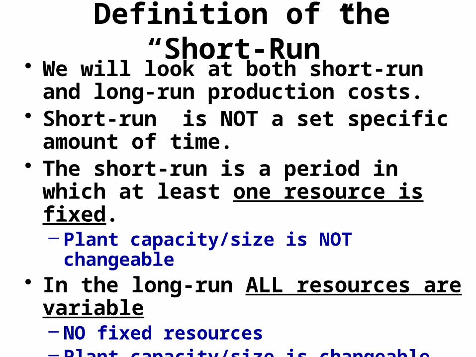
Definition of the “Short-Run”• We will look at both short-run and long-run
production costs.• Short-run is NOT a set specific amount of
time.• The short-run is a period in which at least one
resource is fixed.– Plant capacity/size is NOT changeable
• In the long-run ALL resources are variable– NO fixed resources– Plant capacity/size is changeable
Today we will examine Short-run costs.

Total CostsFC = Total Fixed Costs VC = Total Variable Costs TC = Total Costs
Per Unit CostsAFC = Average Fixed Costs AVC = Average Variable Costs ATC = Average Total Costs MC = Marginal Cost
Different Economic Costs

Fixed Costs:Costs for fixed resources that DON’T change with the amount producedEx: Rent, Insurance, Managers Salaries, etc.
Average Fixed Costs = Fixed CostsQuantity
Variable Costs:Costs for variable resources that DO change as more or less is producedEx: Raw Materials, Labor, Electricity, etc.
Average Variable Costs = Variable CostsQuantity
Definitions
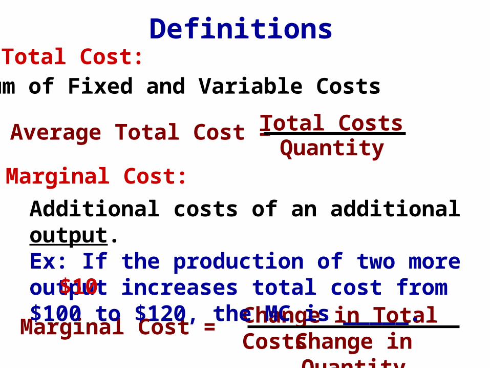
Total Cost:Sum of Fixed and Variable Costs
Average Total Cost = Total CostsQuantity
Marginal Cost:
Marginal Cost = Change in Total CostsChange in Quantity
Additional costs of an additional output.Ex: If the production of two more output increases total cost from $100 to $120, the MC is _____.
Definitions
$10

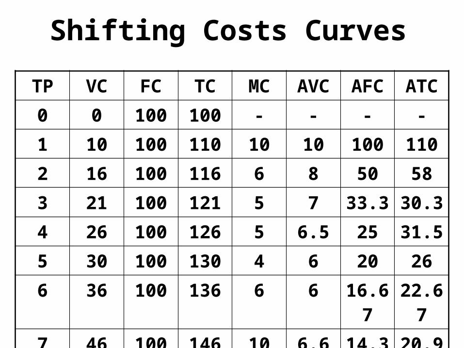
Calculating TC, VC, FC, ATC, AFC, and MC
TP VC FC TC MC AVC AFC ATC0 0 1001 102 163 214 265 306 367 46
Draw this in your notes

Calculating TC, VC, FC, ATC, AFC, and MC
TP VC FC TC MC AVC AFC ATC0 0 1001 10 1002 16 1003 21 1004 26 1005 30 1006 36 1007 46 100

Calculating TC, VC, FC, ATC, AFC, and MC
TP VC FC TC MC AVC AFC ATC0 0 100 1001 10 100 1102 16 100 1163 21 100 1214 26 100 1265 30 100 1306 36 100 1367 46 100 146
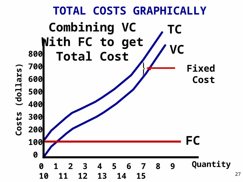
TOTAL COSTS GRAPHICALLY
Quantity
TC
Fixed Cost
VC
FC
Combining VCWith FC to get
Total Cost
0 1 2 3 4 5 6 7 8 9 10 11 12 13 14 15
Co
sts
(do
llar
s)
800
700
600
500
400
300
200
100
0
27

Quantity
Co
sts
(do
llar
s)
TC
Fixed Cost
VC
FC
Combining VCWith FC to get
Total Cost
0 1 2 3 4 5 6 7 8 9 10 11 12 13 14 15
What is the TOTAL COST, FC, and VC for
producing 9 units?
TOTAL COSTS GRAPHICALLY
800
700
600
500
400
300
200
100
0

Per Unit CostsTP VC FC TC MC AVC AFC ATC0 0 100 100 -1 10 100 1102 16 100 1163 21 100 1214 26 100 1265 30 100 1306 36 100 1367 46 100 146

Per Unit CostsTP VC FC TC MC AVC AFC ATC0 0 100 100 -1 10 100 110 102 16 100 116 63 21 100 121 54 26 100 126 55 30 100 130 46 36 100 136 67 46 100 146 10

TP VC FC TC MC AVC AFC ATC0 0 100 100 - -1 10 100 110 10 102 16 100 116 6 83 21 100 121 5 74 26 100 126 5 6.55 30 100 130 4 66 36 100 136 6 67 46 100 146 10 6.6
Per Unit Costs

TP VC FC TC MC AVC AFC ATC0 0 100 100 - - -1 10 100 110 10 10 1002 16 100 116 6 8 503 21 100 121 5 7 33.34 26 100 126 5 6.5 255 30 100 130 4 6 206 36 100 136 6 6 16.677 46 100 146 10 6.6 14.3
Asymptote
Per Unit Costs

TP VC FC TC MC AVC AFC ATC0 0 100 100 - - - -1 10 100 110 10 10 100 1102 16 100 116 6 8 50 583 21 100 121 5 7 33.3 40.34 26 100 126 5 6.5 25 31.55 30 100 130 4 6 20 266 36 100 136 6 6 16.67 22.677 46 100 146 10 6.6 14.3 20.9
Per Unit Costs

TP VC FC TC MC AVC AFC ATC0 0 100 100 - - - -1 10 100 110 10 10 100 1102 16 100 116 6 8 50 583 21 100 121 5 7 33.3 40.34 26 100 126 5 6.5 25 31.55 30 100 130 4 6 20 266 36 100 136 6 6 16.67 22.677 46 100 146 10 6.6 14.3 20.9
Per Unit Costs
34
Quantity
Co
sts
(do
llar
s)
AFC
AVC
ATC
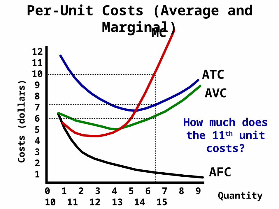
Per-Unit Costs (Average and Marginal)
121110987654321
0 1 2 3 4 5 6 7 8 9 10 11 12 13 14 15
How much does the 11th unit costs?
MC

Quantity
Co
sts
(do
llar
s)
AFC
AVC
ATC
MC
Per-Unit Costs (Average and Marginal)
121110987654321
0 1 2 3 4 5 6 7 8 9 10 11 12 13 14 15
Average Fixed Cost
ATC and AVC get closer and closer but
NEVER touch

Per-Unit Costs (Average and Marginal)
At output Q, what area represents:
TCVCFC
0CDQ0BEQ0AFQ or BCDE

Why is the MC curve U-shaped?
Quantity
Co
sts
(do
llar
s)
MC121110987654321
0 1 2 3 4 5 6 7 8 9 10 11 12 13 14 15
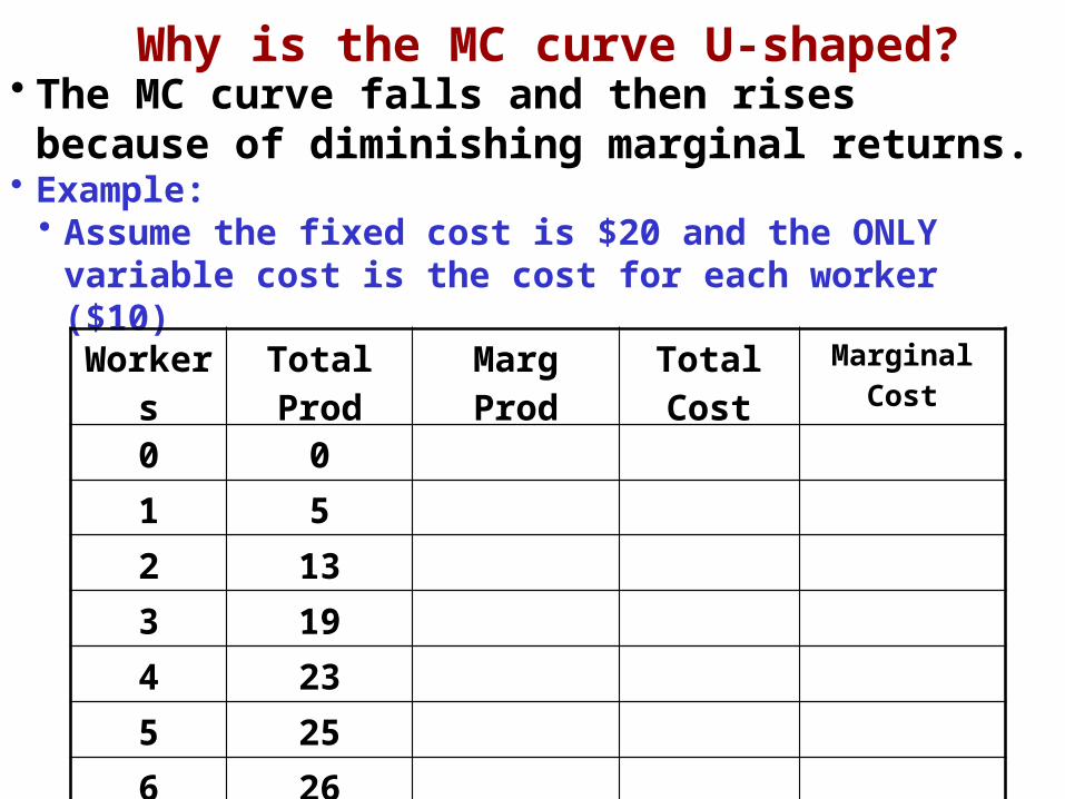
Why is the MC curve U-shaped?• The MC curve falls and then rises because of
diminishing marginal returns.• Example:
• Assume the fixed cost is $20 and the ONLY variable cost is the cost for each worker ($10)
Workers Total Prod Marg Prod Total Cost Marginal Cost
0 0
1 5
2 13
3 19
4 23
5 25
6 26

Workers Total Prod Marg Prod Total Cost Marginal Cost
0 0 -
1 5 5
2 13 8
3 19 6
4 23 4
5 25 2
6 26 1
Why is the MC curve U-shaped?• The MC curve falls and then rises because of
diminishing marginal returns.• Example:
• Assume the fixed cost is $20 and the ONLY variable cost is the cost for each worker ($10)
Workers Total Prod Marg Prod Total Cost Marginal Cost
0 0 - $20
1 5 5 $30
2 13 8 $40
3 19 6 $50
4 23 4 $60
5 25 2 $70
6 26 1 $80
Why is the MC curve U-shaped?• The MC curve falls and then rises because of
diminishing marginal returns.• Example:
• Assume the fixed cost is $20 and the ONLY variable cost is the cost for each worker (Wage = $10)

Workers Total Prod Marg Prod Total Cost Marginal Cost
0 0 - $20 -
1 5 5 $30 10/5 = $2
2 13 8 $40 10/8 = $1.25
3 19 6 $50 10/6 = $1.6
4 23 4 $60 10/4 = $2.5
5 25 2 $70 10/2 = $5
6 26 1 $80 10/1 = $10
Why is the MC curve U-shaped?• The MC curve falls and then rises because of
diminishing marginal returns.• Example:
• Assume the fixed cost is $20 and the ONLY variable cost is the cost for each worker ($10)
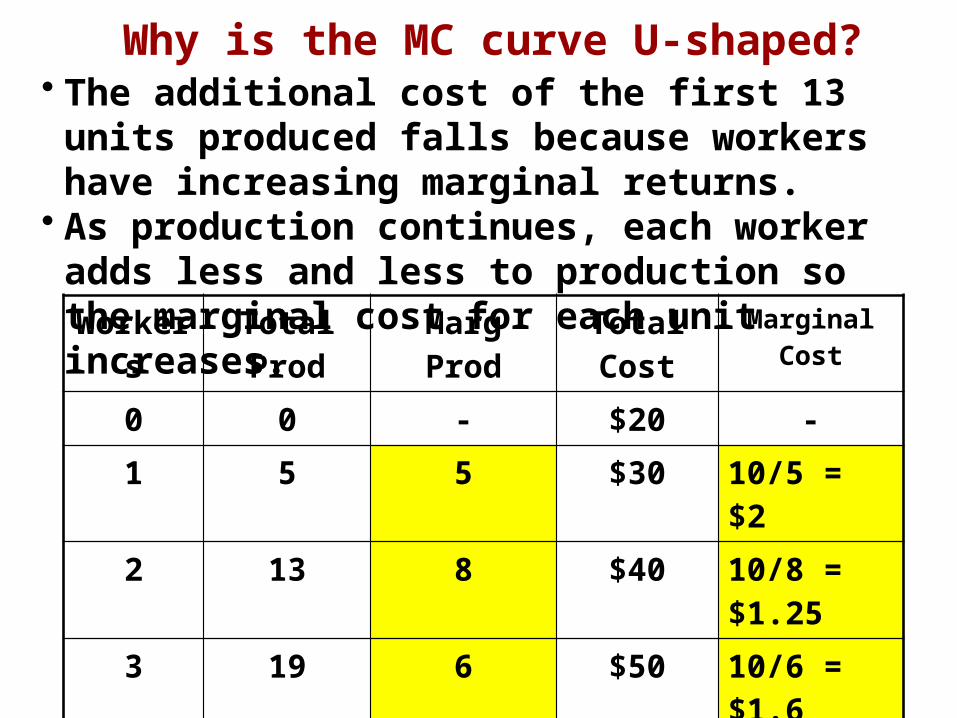
Workers Total Prod Marg Prod Total Cost Marginal Cost
0 0 - $20 -
1 5 5 $30 10/5 = $2
2 13 8 $40 10/8 = $1.25
3 19 6 $50 10/6 = $1.6
4 23 4 $60 10/4 = $2.5
5 25 2 $70 10/2 = $5
6 26 1 $80 10/1 = $10
• The additional cost of the first 13 units produced falls because workers have increasing marginal returns.
• As production continues, each worker adds less and less to production so the marginal cost for each unit increases.
Why is the MC curve U-shaped?

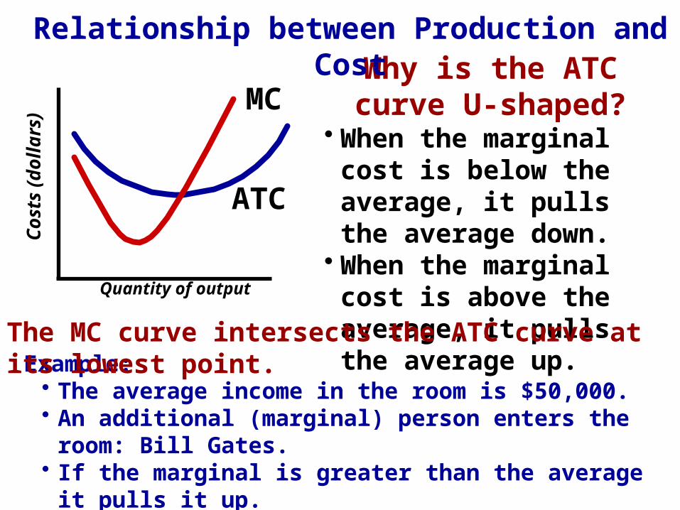
Relationship between Production and CostC
os
ts (
do
llars
)A
vera
ge
pro
du
ct a
nd
mar
gin
al p
rod
uct
Quantity of labor
Quantity of output
MP
MC
Why is the MC curve U-shaped?
• When marginal product is increasing, marginal cost falls.
• When marginal product falls, marginal costs increase.
MP and MC are mirror images of each other.
Co
sts
(d
olla
rs)
Ave
rag
e p
rod
uct
an
dm
arg
inal
pro
du
ct
Quantity of labor
Quantity of output
MP
MC
ATC
Why is the ATC curve U-shaped?
• When the marginal cost is below the average, it pulls the average down.
• When the marginal cost is above the average, it pulls the average up.
Relationship between Production and Cost
Example:• The average income in the room is $50,000.• An additional (marginal) person enters the room: Bill Gates.• If the marginal is greater than the average it pulls it up.• Notice that MC can increase but still pull down the average.
The MC curve intersects the ATC curve at its lowest point.

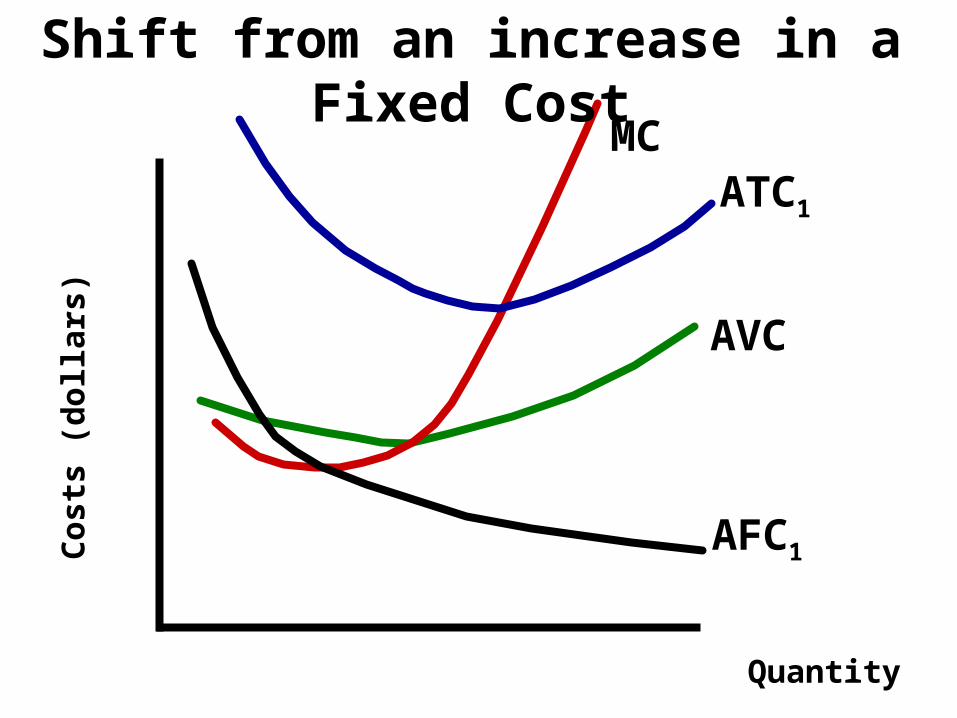
Shifting Cost Curves

Shifting Costs Curves
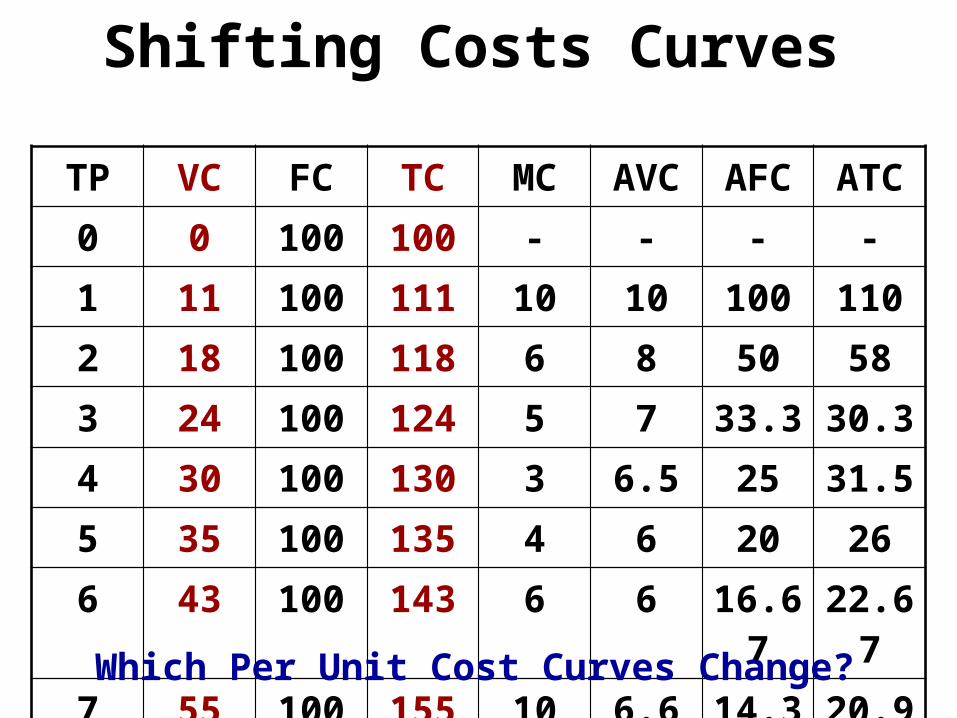
TP VC FC TC MC AVC AFC ATC0 0 100 100 - - - -1 10 100 110 10 10 100 1102 16 100 116 6 8 50 583 21 100 121 5 7 33.3 30.34 26 100 126 3 6.5 25 31.55 30 100 130 4 6 20 266 36 100 136 6 6 16.67 22.677 46 100 146 10 6.6 14.3 20.9
What if Fixed Costs increase to
$200

Shifting Costs Curves
TP VC FC TC MC AVC AFC ATC0 0 100 100 - - - -1 10 100 110 10 10 100 1102 16 100 116 6 8 50 583 21 100 121 5 7 33.3 30.34 26 100 126 5 6.5 25 31.55 30 100 130 4 6 20 266 36 100 136 6 6 16.67 22.677 46 100 146 10 6.6 14.3 20.9

Shifting Costs Curves
TP VC FC TC MC AVC AFC ATC0 0 200 100 - - - -1 10 200 110 10 10 100 1102 16 200 116 6 8 50 583 21 200 121 5 7 33.3 30.34 26 200 126 5 6.5 25 31.55 30 200 130 4 6 20 266 36 200 136 6 6 16.67 22.677 46 200 146 10 6.6 14.3 20.9

Shifting Costs Curves
TP VC FC TC MC AVC AFC ATC0 0 200 200 - - - -1 10 200 210 10 10 100 1102 16 200 216 6 8 50 583 21 200 221 5 7 33.3 30.34 26 200 226 5 6.5 25 31.55 30 200 230 4 6 20 266 36 200 236 6 6 16.67 22.677 46 200 246 10 6.6 14.3 20.9
Which Per Unit Cost Curves Change?

Shifting Costs Curves
TP VC FC TC MC AVC AFC ATC0 0 200 200 - - - -1 10 200 210 10 10 100 1102 16 200 216 6 8 50 583 21 200 221 5 7 33.3 30.34 26 200 226 5 6.5 25 31.55 30 200 230 4 6 20 266 36 200 236 6 6 16.67 22.677 46 200 246 10 6.6 14.3 20.9
ONLY AFC and ATC Increase!

Shifting Costs Curves
TP VC FC TC MC AVC AFC ATC0 0 200 200 - - - -1 10 200 210 10 10 200 1102 16 200 216 6 8 100 583 21 200 221 5 7 66.6 30.34 26 200 226 5 6.5 50 31.55 30 200 230 4 6 40 266 36 200 236 6 6 33.3 22.677 46 200 246 10 6.6 28.6 20.9
ONLY AFC and ATC Increase!

Shifting Costs Curves
TP VC FC TC MC AVC AFC ATC0 0 200 200 - - - -1 10 200 210 10 10 200 2102 16 200 216 6 8 100 1083 21 200 221 5 7 66.6 73.64 26 200 226 5 6.5 50 56.55 30 200 230 4 6 40 466 36 200 236 6 6 33.3 39.37 46 200 246 10 6.6 28.6 35.2
If fixed costs change ONLY AFC and ATC Change!
MC and AVC DON’T change!

Quantity
Co
sts
(do
llar
s)
AFC
AVCATC
MC
Shift from an increase in a Fixed Cost
ATC1
AFC1
Quantity
Co
sts
(do
llar
s)
MC
Shift from an increase in a Fixed Cost
ATC1
AVC
AFC1

Shifting Costs Curves
TP VC FC TC MC AVC AFC ATC0 0 100 100 - - - -1 10 100 110 10 10 100 1102 16 100 116 6 8 50 583 21 100 121 5 7 33.3 30.34 26 100 126 5 6.5 25 31.55 30 100 130 4 6 20 266 36 100 136 6 6 16.67 22.677 46 100 146 10 6.6 14.3 20.9
What if the cost for variable resources
increase
TP VC FC TC MC AVC AFC ATC0 0 100 100 - - - -1 10 100 110 10 10 100 1102 16 100 116 6 8 50 583 21 100 121 5 7 33.3 30.34 26 100 126 5 6.5 25 31.55 30 100 130 4 6 20 266 36 100 136 6 6 16.67 22.677 46 100 146 10 6.6 14.3 20.9
Shifting Costs Curves

TP VC FC TC MC AVC AFC ATC0 0 100 100 - - - -1 11 100 110 10 10 100 1102 18 100 116 6 8 50 583 24 100 121 5 7 33.3 30.34 30 100 126 5 6.5 25 31.55 35 100 130 4 6 20 266 43 100 136 6 6 16.67 22.677 55 100 146 10 6.6 14.3 20.9
Shifting Costs Curves
TP VC FC TC MC AVC AFC ATC0 0 100 100 - - - -1 11 100 111 10 10 100 1102 18 100 118 6 8 50 583 24 100 124 5 7 33.3 30.3
4 30 100 130 3 6.5 25 31.55 35 100 135 4 6 20 266 43 100 143 6 6 16.67 22.677 55 100 155 10 6.6 14.3 20.9
Shifting Costs Curves
Which Per Unit Cost Curves Change?

TP VC FC TC MC AVC AFC ATC0 0 100 100 - - - -1 11 100 111 11 10 100 1102 18 100 118 7 8 50 583 24 100 124 6 7 33.3 30.3
4 30 100 130 6 6.5 25 31.55 35 100 135 5 6 20 266 43 100 143 8 6 16.67 22.677 55 100 155 12 6.6 14.3 20.9
Shifting Costs Curves
MC, AVC, and ATC Change!

TP VC FC TC MC AVC AFC ATC0 0 100 100 - - - -1 11 100 111 11 11 100 1102 18 100 118 7 9 50 583 24 100 124 6 8 33.3 30.3
4 30 100 130 6 7.5 25 31.55 35 100 135 5 7 20 266 43 100 143 8 7.16 16.67 22.677 55 100 155 12 7.8 14.3 20.9
Shifting Costs Curves
MC, AVC, and ATC Change!

TP VC FC TC MC AVC AFC ATC0 0 100 100 - - - -1 11 100 111 11 11 100 1112 18 100 118 7 9 50 593 24 100 124 6 8 33.3 41.3
4 30 100 130 6 7.5 25 32.55 35 100 135 5 7 20 276 43 100 143 8 7.16 16.67 23.837 55 100 155 12 7.8 14.3 22.1
Shifting Costs CurvesIf variable costs change MC, AVC, and ATC Change!

Quantity
Co
sts
(do
llar
s)
AFC
AVCATC
MCATC1
AVC1
Shift from an increase in a Variable CostsMC1

Quantity
Co
sts
(do
llar
s)
AFC
ATC1
AVC1
Shift from an increase in a Variable CostsMC1
Long-Run Costs

In the long run all resources are variable. Plant capacity/size can change.
Definition and Purpose of the Long Run
Why is this important?The Long-Run is used for planning. Firms use to identify
which plant size results in the lowest per unit cost. Ex: Assume a firm is producing 100 bikes with a fixed
number of resources (workers, machines, etc.). If this firm decides to DOUBLE the number of
resources, what will happen to the number of bikes it can produce?
There are only three possible outcomes: 1. Number of bikes will double (constant returns to scale)2. Number of bikes will more than double (economies of scale)3. Number of bikes will less than double (diseconomies of scale)

Long Run ATCWhat happens to the average total costs of a
product when a firm increases its plant capacity?
Example of various plant sizes:• I make looms out of my garage with one saw• I rent out building, buy 5 saws, hire 3 workers• I rent a factor, buy 20 saws and hire 40 workers• I build my own plant and use robots to build looms.• I create plants in every major city in the U.S.
Long Run ATC curve is made up of all the different short run ATC curves of various plant
sizes.

ECONOMIES OF SCALEWhy does economies of scale occur?• Firms that produce more can better use Mass
Production Techniques and Specialization.Example:• A car company that makes 50 cars will have a very
high average cost per car.• A car company that can produce 100,000 cars will
have a low average cost per car.• Using mass production techniques, like robots, will
cause total cost to be higher but the average cost for each car would be significantly lower.

Long Run AVERAGE Total Cost
Quantity Cars
CostsATC1
MC1
0 1 100 1,000 100,000 1,000,0000
$9,900,000
$50,000
$6,000
$3,000

Long Run AVERAGE Total Cost
Quantity Cars
CostsATC1
MC1
MC2
0 1 100 1,000 100,000 1,000,0000
$9,900,000
ATC2
Economies of Scale- Long Run Average Cost falls
because mass production techniques are used.
$50,000
$6,000
$3,000

Long Run AVERAGE Total Cost
Quantity Cars
CostsATC1
MC1
ATC2
MC2
ATC3
MC3
0 1 100 1,000 100,000 1,000,0000
$9,900,000
$50,000
$6,000
$3,000
Economies of Scale- Long Run Average Cost falls
because mass production techniques are used.
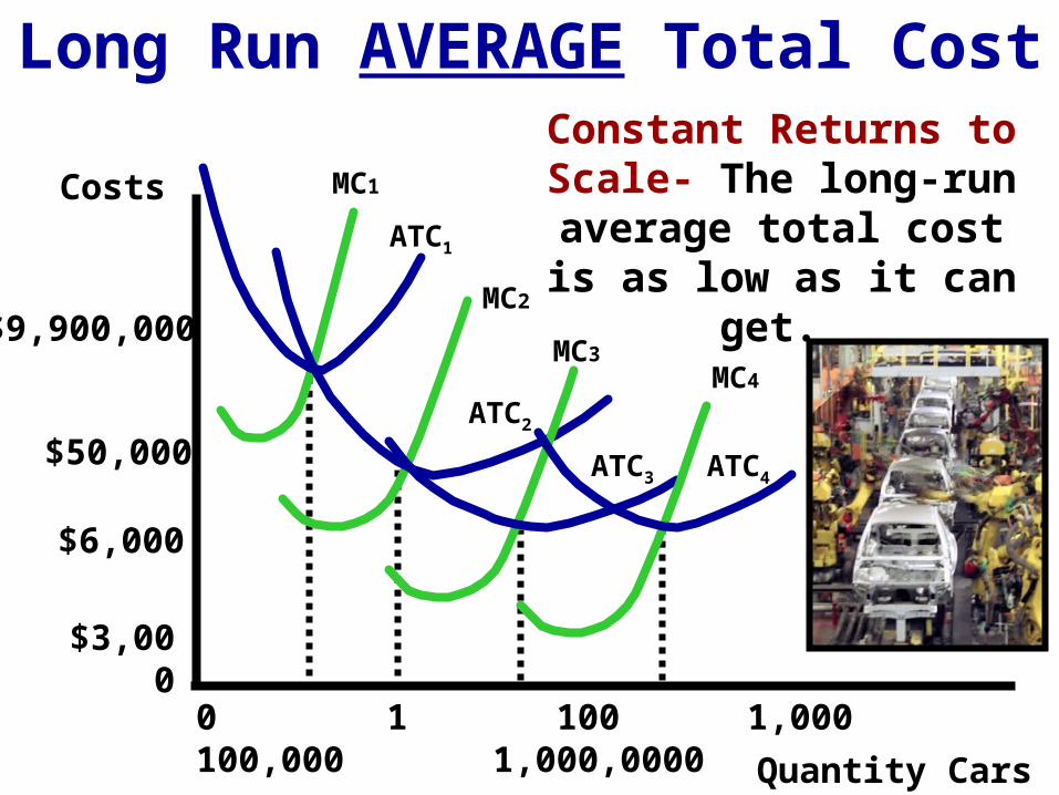
Long Run AVERAGE Total Cost
Quantity Cars
CostsATC1
MC1
ATC2
MC2
ATC3
MC3
0 1 100 1,000 100,000 1,000,0000
$9,900,000
$50,000
$6,000
$3,000
Constant Returns to Scale- The long-run average total cost is as low as it can get.
MC4
ATC4

Long Run AVERAGE Total Cost
Quantity Cars
CostsATC1
MC1
ATC2
MC2
ATC3
MC3MC5
0 1 100 1,000 100,000 1,000,0000
$9,900,000MC4 ATC5
$6,000
$3,000
ATC4
Diseconomies of Scale- Long run cost increase as the firm gets too big and
difficult to manage.
$50,000

Long Run AVERAGE Total Cost
Quantity Cars
CostsATC1
MC1
ATC2
MC2
ATC3
MC3MC5
0 1 100 1,000 100,000 1,000,0000
$9,900,000MC4 ATC5
$6,000
$3,000
ATC4
Diseconomies of Scale- The LRATC is increasing as the
firm gets too big and difficult to manage.
$50,000

Long Run AVERAGE Total Cost
Quantity Cars
CostsATC1
MC1
ATC2
MC2
ATC3
MC3MC5
0 1 100 1,000 100,000 1,000,0000
$9,900,000MC4 ATC5
$6,000
$3,000
ATC4
These are all short run average costs curves.
Where is the Long Run Average Cost Curve?
$50,000

Long Run AVERAGE Total Cost
Quantity Cars
Costs
0 1 100 1,000 100,000 1,000,0000
Long Run Average Cost
Curve
Economies of Scale
Constant Returns to
Scale
Diseconomies of Scale

LRATC Simplified
Quantity
Costs
Long Run Average Cost
Curve
Economies of Scale
Constant Returns to Scale
Diseconomies of Scale
The law of diminishing marginal returns doesn’t apply in the long run because there are no FIXED RESOURCES.


