SANDIA REPORT SAND2015-8849 Unlimited Release Printed September 2015 Microgrid Design Toolkit (MDT) Technical Documentation and Component Summaries Bryan Arguello, John Eddy, Jared Gearhart, Katherine Jones Prepared by Sandia National Laboratories Albuquerque, New Mexico 87185 and Livermore, California 94550 Sandia National Laboratories is a multi-program laboratory managed and operated by Sandia Corporation, a wholly owned subsidiary of Lockheed Martin Corporation, for the U.S. Department of Energy's National Nuclear Security Administration under contract DE-AC04-94AL85000. Approved for public release; further dissemination unlimited.
Transcript
SANDIA REPORTSAND2015-8849Unlimited ReleasePrinted September 2015
Microgrid Design Toolkit (MDT)Technical Documentation and Component Summaries
Bryan Arguello, John Eddy, Jared Gearhart, Katherine Jones
Prepared bySandia National LaboratoriesAlbuquerque, New Mexico 87185 and Livermore, California 94550
Sandia National Laboratories is a multi-program laboratory managed and operated by Sandia Corporation, a wholly owned subsidiary of Lockheed Martin Corporation, for the U.S. Department of Energy's National Nuclear Security Administration under contract DE-AC04-94AL85000.
Approved for public release; further dissemination unlimited.
2
Issued by Sandia National Laboratories, operated for the United States Department of Energy by Sandia Corporation.
NOTICE: This report was prepared as an account of work sponsored by an agency of the United States Government. Neither the United States Government, nor any agency thereof, nor any of their employees, nor any of their contractors, subcontractors, or their employees, make any warranty, express or implied, or assume any legal liability or responsibility for the accuracy, completeness, or usefulness of any information, apparatus, product, or process disclosed, or represent that its use would not infringe privately owned rights. Reference herein to any specific commercial product, process, or service by trade name, trademark, manufacturer, or otherwise, does not necessarily constitute or imply its endorsement, recommendation, or favoring by the United States Government, any agency thereof, or any of their contractors or subcontractors. The views and opinions expressed herein do not necessarily state or reflect those of the United States Government, any agency thereof, or any of their contractors.
Printed in the United States of America. This report has been reproduced directly from the best available copy.
Available to DOE and DOE contractors fromU.S. Department of EnergyOffice of Scientific and Technical InformationP.O. Box 62Oak Ridge, TN 37831
Microgrid Design Toolkit (MDT)Technical Documentation and Component
Summaries
Bryan ArguelloJared Gearhart
Katherine JonesOperations Research and Computational Analysis
John EddySystems Readiness and Sustainment Technology
Sandia National LaboratoriesP.O. Box 5800
Albuquerque, New Mexico 87185-MS1188
Abstract
The Microgrid Design Toolkit (MDT) is a decision support software tool for microgrid designers to use during the microgrid design process. The models that support the two main capabilities in MDT are described. The first capability, the Microgrid Sizing Capability (MSC), is used to determine the size and composition of a new microgrid in the early stages of the design process. MSC is a mixed-integer linear program that is focused on developing a microgrid that is economically viable when connected to the grid. The second capability is focused on refining a microgrid design for operation in islanded mode. This second capability relies on two models: the Technology Management Optimization (TMO) model and Performance Reliability Model (PRM). TMO uses a genetic algorithm to create and refine a collection of candidate microgrid designs. It uses PRM, a simulation based reliability model, to assess the performance of these designs. TMO produces a collection of microgrid designs that perform well with respect to one or more performance metrics.
FIGURESFigure 1. Illustration of a Pareto Optimal Frontier. .......................................................................31Figure 2. TMO Optimization Framework. ....................................................................................32Figure 3. General form of normalizing functions for metrics that are to be maximized and minimized ......................................................................................................................................38Figure 4. General form of normalizing functions for metrics with a seek value improvement type.......................................................................................................................................................38Figure 5. Illustrative example showing the crossover technique used in the MDT GA................39Figure 6: Phases of simulation in PRM .........................................................................................43Figure 7: Illustration of an example path in PRM .........................................................................44
TABLESTable 1. MSC Indices ....................................................................................................................13Table 2. Demand Input Data..........................................................................................................13Table 3. Market Input Data............................................................................................................14Table 4. Distributed Energy Resource Technologies Input Data ..................................................14Table 5. Other Input Parameters ....................................................................................................16
6
Table 6. MSC Decision Variables .................................................................................................17Table 7. Equipment Types and Associated Data ...........................................................................33Table 8. Equipment Attached to Buses in MDT and Associated Data..........................................34Table 9. Summary of MDT Metrics ..............................................................................................36
7
NOMENCLATURE
AC Alternating CurrentAC-OPF AC Optimal Power FlowAPI Application Programming InterfaceDC Direct CurrentDER Distributed Energy ResourcesDER-CAM Distributed Energy Resources Customer Adoption ModelDOE Department of EnergyGA Genetic AlgorithmMDT Microgrid Design ToolkitMILP Mixed-Integer Linear ProgramMSC Microgrid Sizing CapabilityPRM Performance and Reliability ModelTMO Technology Management OptimizationUOM Unit of MeasureUPS Uninterruptable Power Supply
8
9
1. INTRODUCTION
The Microgrid Design Toolkit (MDT) is a decision support software tool for microgrid designers to use during the microgrid design process. MDT is funded by the Department of Energy (DOE) with the intent of encouraging the adoption of microgrid technologies. The integrated MDT is a new system architecture which leverages the capabilities of several existing software tools. The current version of MDT includes two main capabilities. The first capability, the Microgrid Sizing Capability (MSC), is used to determine the size and composition of a new microgrid in the early stages of the design process. MSC is focused on developing a microgrid that is economically viable when connected to the grid. The second capability is focused on refining a microgrid design for operation in islanded mode. This second capability relies on two models: the Technology Management Optimization (TMO) model and Performance Reliability Model (PRM).
MSC is intended to be used early in the microgrid design process to assist analysts with making an initial determination of the types and quantities of technology to be purchased for use in a microgrid. It can also be used to assess the feasibility of developing a microgrid. MSC recommends the combination of technologies that produces the greatest reduction in annual costs compared to purchasing all energy from the utility provider. MSC ensures that the microgrid will pay for itself through annual energy savings within a user-specified amount of time. In addition to recommending the technologies to purchase, MSC provides an estimate of the annual costs (operating and capital) and an estimate of the annual savings associated with the microgrid. After using MSC to make an initial determination of the size and composition of the microgrid, more detailed analysis can be performed to determine the details (e.g. the topology) of the microgrid.
The second capability uses TMO and PRM to refine a microgrid design for optimal performance in islanded mode operation. This capability is intended to be used in the latter stages of the microgrid design process. At this point in the process, the topology of the microgrid should mostly be defined and the main decisions to be made will be details about the design. This could include determining whether or not to add a specific technology at a bus or choosing between several types of technologies to fulfill a predefined need in the microgrid.
TMO is an optimization model that is used to identify which combinations of technologies should be selected for use in a baseline microgrid design. It performs a multi-objective search to provide tradeoff information over multiple dimensions. Examples of the objectives included in TMO are cost, performance, and reliability. The result of TMO is a collection of microgrid designs that each highlights different regions of the trade space. In order quantify certain objectives, it is necessary to model the performance of a selected microgrid. The purpose of PRM is to simulate and quantify microgrid electrical performance in islanded mode given knowledge about the reliability of individual components and a topology specification. These performance evaluations are then used by TMO to explore the cost/performance trade space.
10
Purchases recommended by MSC are not directly transferable to TMO. MSC is used in the early stages of the design process to determine the initial size of a microgrid design with a focus on operating in grid connected mode. Before TMO can be used, the topology and other details of microgrid design must be determined. Once these intermediate steps have been completed TMO can be used to refine the microgrid design to improve performance in islanded mode operation.
11
2. MICROGRID SIZING CAPABILITY
The purpose of MSC is to assist analysts with making an initial determination of the size and composition of a new microgrid. The MSC capability in MDT currently considers investments in distributed generation technologies, photovoltaics, wind generators, and batteries. The model recommends the combination of these technologies that produces the greatest reduction in annual costs compared to the base case where all energy is purchased from the utility. The MSC model is based on the Distributed Energy Resources Customer Adoption Model (DER-CAM).1 Several updates, including the addition of wind, have been made to tailor the DER-CAM model to MDT.
The key strength of MSC is that it can help analysts understand the feasibility and benefits of developing a microgrid prior to performing more detailed analyses. The main inputs required for an MSC analysis are electric load data for the site under consideration, market cost data for the electric utility company, and a collection of technologies under consideration for use in the microgrid (with the associated technical and cost data). However, MSC is only the first step in the microgrid design process. Since it is a high level model that is primarily focused on minimizing cost, additional analysis is required to determine the topology, design details, and operating policies for the microgrid.
MSC uses optimization to determine the initial microgrid design. Specifically, the model created by MSC is a mixed-integer linear program (MILP). There are several benefits associated with this type of model. First, it is transparent since the logic in the model can be represented by a concise set of mathematical expressions. Second, there are efficient algorithms for solving this class of problems. Third, the recommendations of the model are defensible since optimality can be proven for solutions.
When an MSC analysis is performed, the model is solved twice. In the first iteration, no microgrid technology purchases are allowed so that the cost of purchasing enough electricity from the grid can be determined. This cost is necessary so that when purchases are allowed in the second iteration, the model will ensure that the annual energy cost with the microgrid is lower than the annual cost without a microgrid. The annual costs considered in the second iteration of the problem include both operating costs and annualized capital costs. Furthermore, the savings produced by the microgrid must be large enough so that purchases are paid back within a reasonable timeframe.
There are two groups of outputs from MSC: the microgrid technology purchase choices and the associated cost data. The purchase choices include the types and quantities of microgrid
1 Stadler, Michael, Chris Marnay, Afzal S. Siddiqui, Judy Lai, Brian Coffey, and Hirohisa Aki, “Effect of Heat and Electricity Storage and Reliability on Microgrid Viability: A Study of Commercial Buildings in California and New York States,” LBNL-1334E, 2008, available at https://building-microgrid.lbl.gov/publications/effect-heat-and-electricity-storage, accessed June 24, 2015.
technologies purchased. The cost data includes the total capital costs of the purchased technologies, the total annual cost of the microgrid and the annual savings with the microgrid. The total annual cost includes both operating costs and annualized capital costs.
2.1 MSC InputsIn order to perform the technology sizing optimization, MSC requires a user to provide a number of inputs that describe the market costs of electricity, costs of technology, customer load, technology characteristics, solar and wind profiles, and purchase limits.
The market costs associated with electricity in MSC include monthly charges, usage charges, demand charges, and carbon taxes. A monthly charge is collected by the utility for just being connected to the grid, whereas a usage charge is proportional to the amount of electricity purchased from the grid. Demand charges are proportional to the maximum amount of electricity purchased from the grid over a fixed time interval. There can be both daily and monthly demand charges. In addition, the customer also incurs a charge proportional to the maximum electricity load over the full year. MSC calculates the carbon tax by using an emission rate and emission charge along with an electricity load input from the user. If the utility company allows customers to sell electricity back to the grid, MSC will account for savings due to electricity sold back to the grid.
Additionally, the various costs for the different technologies must be specified. Technologies have upfront capital costs, fixed monthly costs, and variable costs. For distributed energy resources (DER) that use fuel, the user can input fuel costs. For generation technologies, there can be a standby charge, proportional to the energy capacity purchased, which is charged by the utility company in exchange for being prepared to compensate for power failures from those technologies.
Analysts may wish to place a limit on usage and quantity purchased for various DER technologies. MSC allows the user to input these quantities, and it makes sure to not violate these limits by adding constraints to the model. For example, for photovoltaics there may be limits on the number of available square feet where this technology could be installed.
For the microgrid technologies under consideration, MSC requires the user to input various technology characteristics. Such characteristics include efficiencies and nameplate capacities--the maximum power output rated by the manufacturer—along with an estimate of the fraction of nameplate capacity actually output by the technology. Representative wind and solar profiles must be provided to determine from the energy output from wind generation and photovoltaic systems.
Finally, MSC will not recommend purchasing a microgrid unless the total savings over a user-specified payback period exceeds the total upfront cost. In order to make this determination, MSC requires the user to input the technology lifetimes, the interest rate on purchases, and a payback period.
13
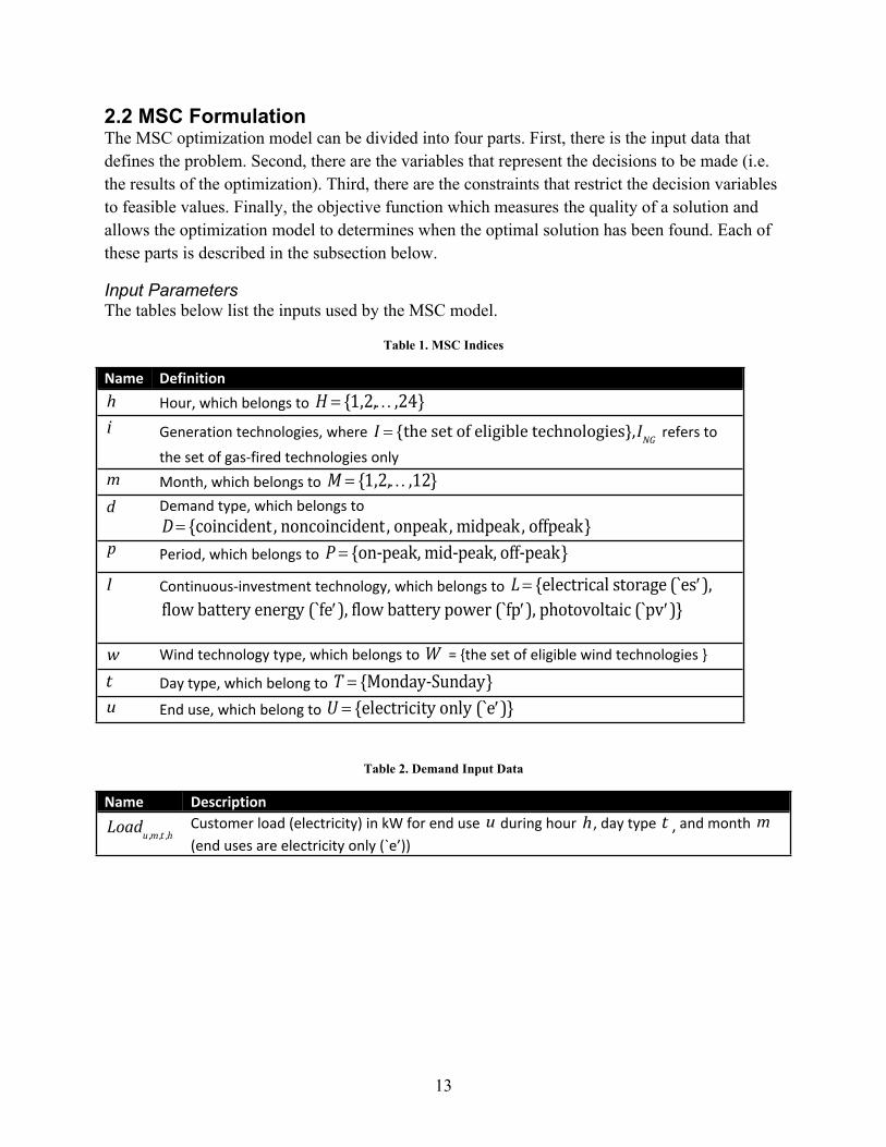
2.2 MSC FormulationThe MSC optimization model can be divided into four parts. First, there is the input data that defines the problem. Second, there are the variables that represent the decisions to be made (i.e. the results of the optimization). Third, there are the constraints that restrict the decision variables to feasible values. Finally, the objective function which measures the quality of a solution and allows the optimization model to determines when the optimal solution has been found. Each of these parts is described in the subsection below.
Input ParametersThe tables below list the inputs used by the MSC model.
Table 1. MSC Indices
Name Definition
h Hour, which belongs to H {1,2,,24} i Generation technologies, where I {the set of eligible technologies},ING refers to
the set of gas-fired technologies only
m Month, which belongs to M {1,2,,12} d Demand type, which belongs to
D {coincident , noncoincident, onpeak, midpeak, offpeak} p Period, which belongs to P {on-peak, mid-peak, off-peak}
l Continuous-investment technology, which belongs to L {electrical storage (`e s ),
flow battery energy (`f e ), flow battery power (`f p ), photovoltaic (`p v )}
w Wind technology type, which belongs to W = {the set of eligible wind technologies }
t Day type, which belong to T {Monday-Sunday} u End use, which belong to U {electricity only (` e )}
Table 2. Demand Input Data
Name Description
Loadu ,m ,t ,h
Customer load (electricity) in kW for end use u during hour h, day type t , and month m (end uses are electricity only (`e’))
14
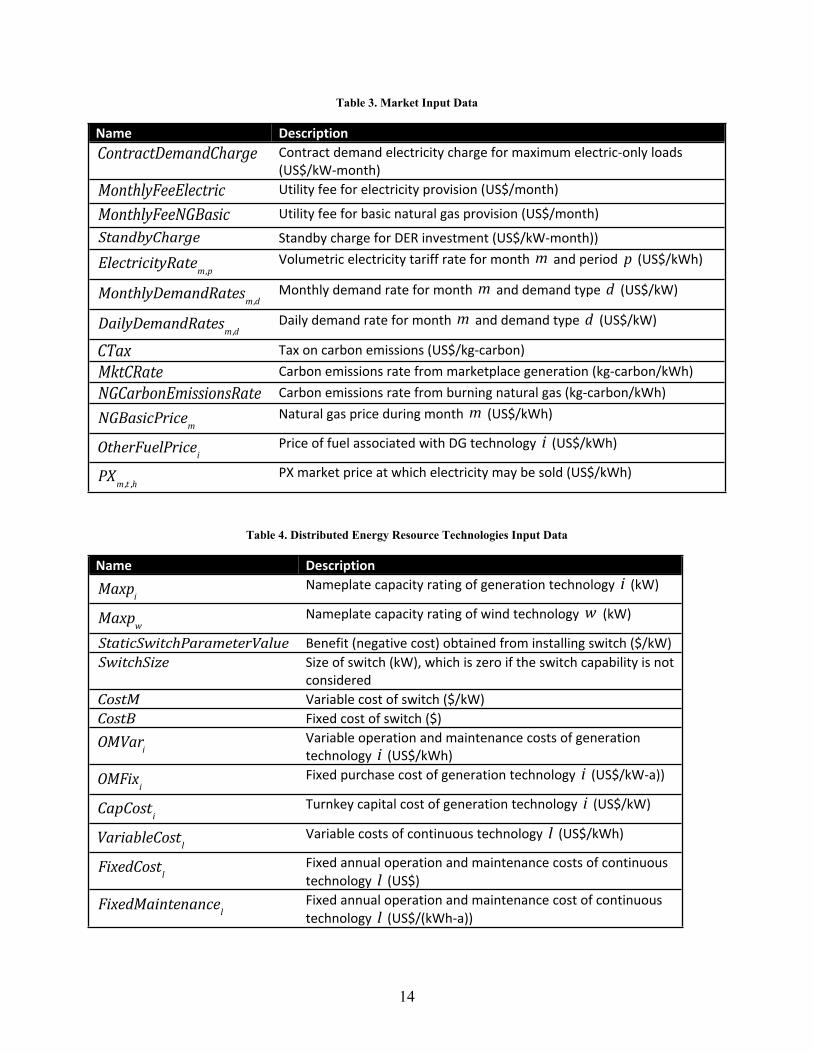
Table 3. Market Input Data
Name DescriptionContractDemandCharge Contract demand electricity charge for maximum electric-only loads
(US$/kW-month)MonthlyFeeElectric Utility fee for electricity provision (US$/month)
MonthlyFeeNGBasic Utility fee for basic natural gas provision (US$/month)
StandbyCharge Standby charge for DER investment (US$/kW-month))
ElectricityRatem,pVolumetric electricity tariff rate for month m and period p (US$/kWh)
MonthlyDemandRatesm,dMonthly demand rate for month m and demand type d (US$/kW)
DailyDemandRatesm,dDaily demand rate for month m and demand type d (US$/kW)
CTax Tax on carbon emissions (US$/kg-carbon)MktCRate Carbon emissions rate from marketplace generation (kg-carbon/kWh)NGCarbonEmissionsRate Carbon emissions rate from burning natural gas (kg-carbon/kWh)
NGBasicPricemNatural gas price during month m (US$/kWh)
OtherFuelPriceiPrice of fuel associated with DG technology i (US$/kWh)
PXm,t ,hPX market price at which electricity may be sold (US$/kWh)
Table 4. Distributed Energy Resource Technologies Input Data
Name Description
MaxpiNameplate capacity rating of generation technology i (kW)
MaxpwNameplate capacity rating of wind technology w (kW)
StaticSwitchParameterValue Benefit (negative cost) obtained from installing switch ($/kW)SwitchSize Size of switch (kW), which is zero if the switch capability is not
consideredCostM Variable cost of switch ($/kW)CostB Fixed cost of switch ($)
OMVariVariable operation and maintenance costs of generation technology i (US$/kWh)
OMFixiFixed purchase cost of generation technology i (US$/kW-a))
CapCostiTurnkey capital cost of generation technology i (US$/kW)
VariableCostlVariable costs of continuous technology l (US$/kWh)
FixedCostlFixed annual operation and maintenance costs of continuous technology l (US$)
FixedMaintenancelFixed annual operation and maintenance cost of continuous technology l (US$/(kWh-a))
15
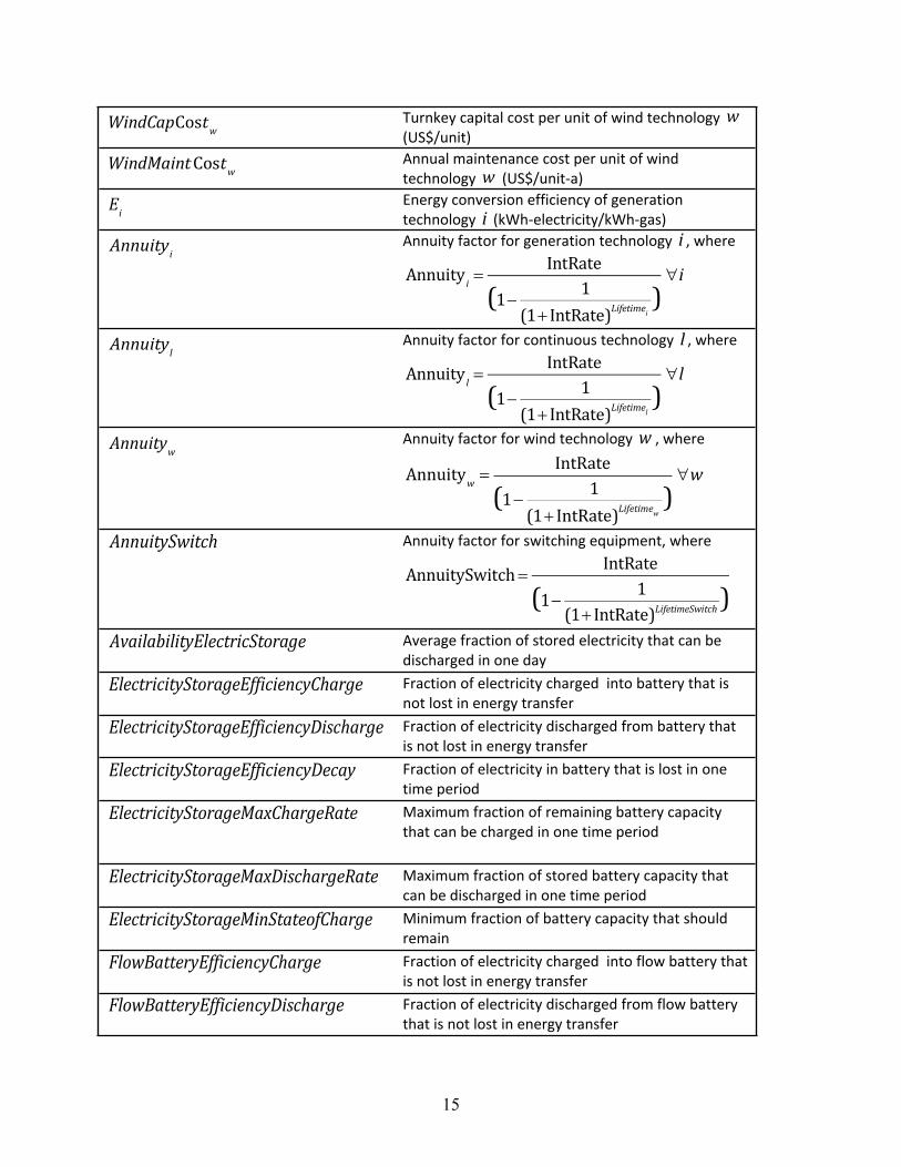
WindCapCostwTurnkey capital cost per unit of wind technology w (US$/unit)
WindMaint CostwAnnual maintenance cost per unit of wind technology w (US$/unit-a)
EiEnergy conversion efficiency of generation technology i (kWh-electricity/kWh-gas)
AnnuityiAnnuity factor for generation technology i , where
Annuity i IntRate
(1 1(1 IntRate)Lifetimei
)i
AnnuitylAnnuity factor for continuous technology l , where
Annuity l IntRate
(1 1(1 IntRate)Lifetimel
)l
AnnuitywAnnuity factor for wind technology w , where
Annuityw IntRate
(1 1(1 IntRate)Lifetimew
)w
AnnuitySwitch Annuity factor for switching equipment, where
AnnuitySwitch IntRate
(1 1(1 IntRate)LifetimeSwitch )
AvailabilityElectricStorage Average fraction of stored electricity that can be discharged in one day
ElectricityStorageEfficiencyCharge Fraction of electricity charged into battery that is not lost in energy transfer
ElectricityStorageEfficiencyDischarge Fraction of electricity discharged from battery that is not lost in energy transfer
ElectricityStorageEfficiencyDecay Fraction of electricity in battery that is lost in one time period
ElectricityStorageMaxChargeRate Maximum fraction of remaining battery capacity that can be charged in one time period
ElectricityStorageMaxDischargeRate Maximum fraction of stored battery capacity that can be discharged in one time period
ElectricityStorageMinStateofCharge Minimum fraction of battery capacity that should remain
FlowBatteryEfficiencyCharge Fraction of electricity charged into flow battery that is not lost in energy transfer
FlowBatteryEfficiencyDischarge Fraction of electricity discharged from flow battery that is not lost in energy transfer
16
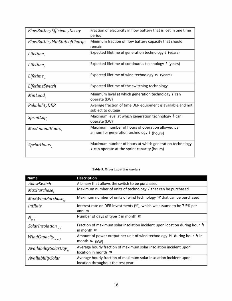
Table 5. Other Input Parameters
Name Description
AllowSwitch A binary that allows the switch to be purchased
MaxPurchaseiMaximum number of units of technology i that can be purchased
MaxWindPurchasewMaximum number of units of wind technology w that can be purchased
IntRate Interest rate on DER investments (%), which we assume to be 7.5% per annum
Nm ,t
Number of days of type t in month m
SolarInsolationm,h
Fraction of maximum solar insolation incident upon location during hour h in month m
WindCapacityw ,m,h
Amount of power output per unit of wind technology w during hour h in month m (kW)
AvailabilitySolarDaymAverage hourly fraction of maximum solar insolation incident upon location in month m
AvailabilitySolar Average hourly fraction of maximum solar insolation incident upon location throughout the test year
FlowBatteryEfficiencyDecay Fraction of electricity in flow battery that is lost in one time period
FlowBatteryMinStateofCharge Minimum fraction of flow battery capacity that should remain
LifetimeiExpected lifetime of generation technology i (years)
LifetimelExpected lifetime of continuous technology l (years)
LifetimewExpected lifetime of wind technology w (years)
LifetimeSwitch Expected lifetime of the switching technology
MinLoadiMinimum level at which generation technology i can operate (kW)
ReliabilityDER Average fraction of time DER equipment is available and not subject to outage
SprintCapiMaximum level at which generation technology i can operate (kW)
MaxAnnualHoursiMaximum number of hours of operation allowed per annum for generation technology i (hours)
SprintHoursiMaximum number of hours at which generation technology i can operate at the sprint capacity (hours)
17
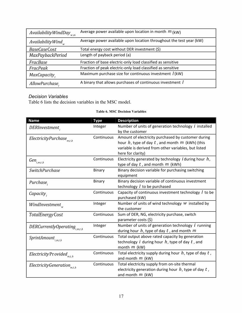
AvailabilityWindDayw ,m
Average power available upon location in month m (kW)
AvailabilityWindwAverage power available upon location throughout the test year (kW)
BaseCaseCost Total energy cost without DER investment ($)
MaxPaybackPeriod Length of payback period (a)
FracBase Fraction of base electric-only load classified as sensitive
FracPeak Fraction of peak electric-only load classified as sensitive
MaxCapacitylMaximum purchase size for continuous investment l (kW)
AllowPurchaselA binary that allows purchases of continuous investment l
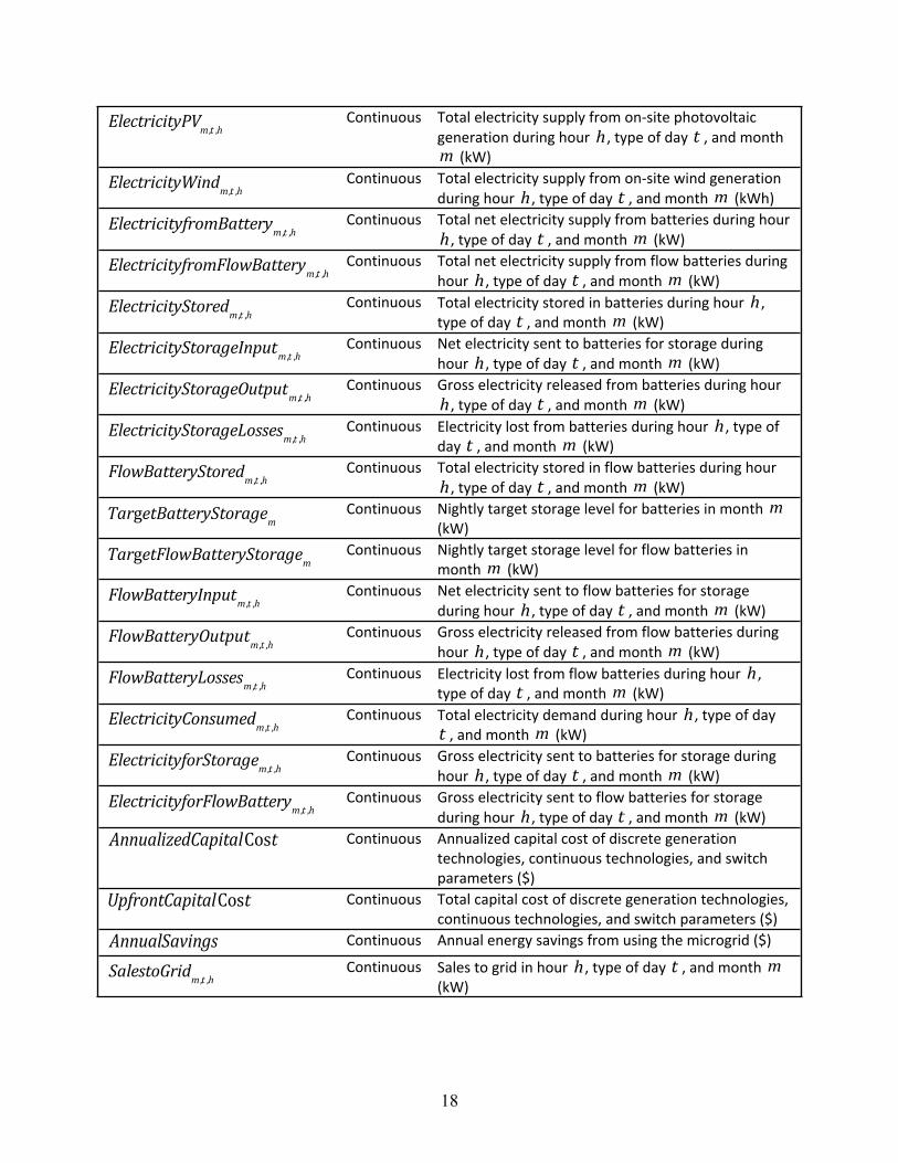
Decision VariablesTable 6 lists the decision variables in the MSC model.
Table 6. MSC Decision Variables
Name Type Description
DERInvestment iInteger Number of units of generation technology i installed
by the customer
ElectricityPurchasem ,t ,h
Continuous Amount of electricity purchased by customer during hour h, type of day t , and month m (kWh) (this variable is derived from other variables, but listed here for clarity)
Geni ,m ,t ,h
Continuous Electricity generated by technology i during hour h, type of day t , and month m (kWh)
SwitchPurchase Binary Binary decision variable for purchasing switching equipment
PurchaselBinary Binary decision variable of continuous investment
technology l to be purchased
CapacitylContinuous Capacity of continuous investment technology l to be
purchased (kW)
WindInvestmentwInteger Number of units of wind technology w installed by
the customer
TotalEnergyCost Continuous Sum of DER, NG, electricity purchase, switch parameter costs ($)
DERCurrentlyOperatingi ,m ,t ,h
Integer Number of units of generation technology i running during hour h, type of day t , and month m
SprintAmounti ,m,t ,hContinuous Total output above rated capacity by generation
technology i during hour h, type of day t , and month m (kW)
ElectricityProvidedm ,t ,h
Continuous Total electricity supply during hour h, type of day t , and month m (kW)
ElectricityGenerationm ,t ,h
Continuous Total electricity supply from on-site thermal electricity generation during hour h, type of day t , and month m (kW)
18
ElectricityPVm,t ,h
Continuous Total electricity supply from on-site photovoltaic generation during hour h, type of day t , and month m (kW)
ElectricityWindm,t ,h
Continuous Total electricity supply from on-site wind generation during hour h, type of day t , and month m (kWh)
ElectricityfromBatterym ,t ,h
Continuous Total net electricity supply from batteries during hour h, type of day t , and month m (kW)
ElectricityfromFlowBatterym ,t ,h
Continuous Total net electricity supply from flow batteries during hour h, type of day t , and month m (kW)
ElectricityStoredm ,t ,h
Continuous Total electricity stored in batteries during hour h, type of day t , and month m (kW)
ElectricityStorageInputm ,t ,h
Continuous Net electricity sent to batteries for storage during hour h, type of day t , and month m (kW)
ElectricityStorageOutputm ,t ,h
Continuous Gross electricity released from batteries during hour h, type of day t , and month m (kW)
ElectricityStorageLossesm ,t ,h
Continuous Electricity lost from batteries during hour h, type of day t , and month m (kW)
FlowBatteryStoredm ,t ,h
Continuous Total electricity stored in flow batteries during hour h, type of day t , and month m (kW)
TargetBatteryStoragemContinuous Nightly target storage level for batteries in month m
(kW)
TargetFlowBatteryStoragemContinuous Nightly target storage level for flow batteries in
month m (kW)
FlowBatteryInputm ,t ,h
Continuous Net electricity sent to flow batteries for storage during hour h, type of day t , and month m (kW)
FlowBatteryOutputm,t ,hContinuous Gross electricity released from flow batteries during
hour h, type of day t , and month m (kW)
FlowBatteryLossesm ,t ,h
Continuous Electricity lost from flow batteries during hour h, type of day t , and month m (kW)
ElectricityConsumedm ,t ,h
Continuous Total electricity demand during hour h, type of day t , and month m (kW)
ElectricityforStoragem ,t ,h
Continuous Gross electricity sent to batteries for storage during hour h, type of day t , and month m (kW)
ElectricityforFlowBatterym ,t ,h
Continuous Gross electricity sent to flow batteries for storage during hour h, type of day t , and month m (kW)
AnnualizedCapitalCost Continuous Annualized capital cost of discrete generation technologies, continuous technologies, and switch parameters ($)
UpfrontCapitalCost Continuous Total capital cost of discrete generation technologies, continuous technologies, and switch parameters ($)
AnnualSavings Continuous Annual energy savings from using the microgrid ($)
SalestoGridm ,t ,h
Continuous Sales to grid in hour h, type of day t , and month m (kW)
19
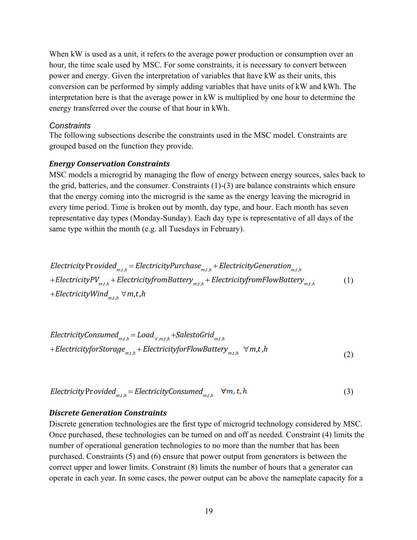
When kW is used as a unit, it refers to the average power production or consumption over an hour, the time scale used by MSC. For some constraints, it is necessary to convert between power and energy. Given the interpretation of variables that have kW as their units, this conversion can be performed by simply adding variables that have units of kW and kWh. The interpretation here is that the average power in kW is multiplied by one hour to determine the energy transferred over the course of that hour in kWh.
ConstraintsThe following subsections describe the constraints used in the MSC model. Constraints are grouped based on the function they provide.
Energy Conservation ConstraintsMSC models a microgrid by managing the flow of energy between energy sources, sales back to the grid, batteries, and the consumer. Constraints (1)-(3) are balance constraints which ensure that the energy coming into the microgrid is the same as the energy leaving the microgrid in every time period. Time is broken out by month, day type, and hour. Each month has seven representative day types (Monday-Sunday). Each day type is representative of all days of the same type within the month (e.g. all Tuesdays in February).
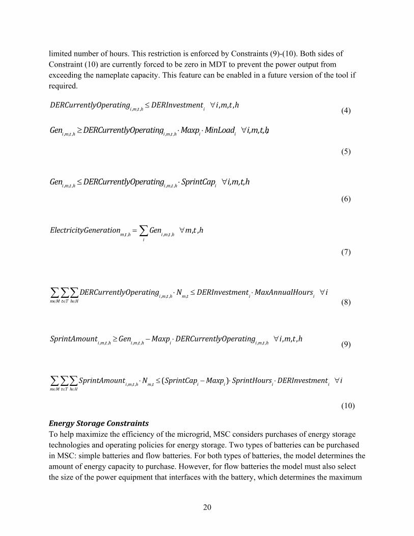
Discrete Generation ConstraintsDiscrete generation technologies are the first type of microgrid technology considered by MSC. Once purchased, these technologies can be turned on and off as needed. Constraint (4) limits the number of operational generation technologies to no more than the number that has been purchased. Constraints (5) and (6) ensure that power output from generators is between the correct upper and lower limits. Constraint (8) limits the number of hours that a generator can operate in each year. In some cases, the power output can be above the nameplate capacity for a
20
limited number of hours. This restriction is enforced by Constraints (9)-(10). Both sides of Constraint (10) are currently forced to be zero in MDT to prevent the power output from exceeding the nameplate capacity. This feature can be enabled in a future version of the tool if required.
DERCurrentlyOperatingi ,m,t ,h DERInvestmenti i ,m,t ,h(4)
mM printAmounti ,m,t ,h Nm,t (SprintCapi Maxpi )SprintHoursi DERInvestmenti i
(10)
Energy Storage ConstraintsTo help maximize the efficiency of the microgrid, MSC considers purchases of energy storage technologies and operating policies for energy storage. Two types of batteries can be purchased in MSC: simple batteries and flow batteries. For both types of batteries, the model determines the amount of energy capacity to purchase. However, for flow batteries the model must also select the size of the power equipment that interfaces with the battery, which determines the maximum
21
charging and discharging rate. Currently, only flow batteries are exposed to the user in the MSC application.
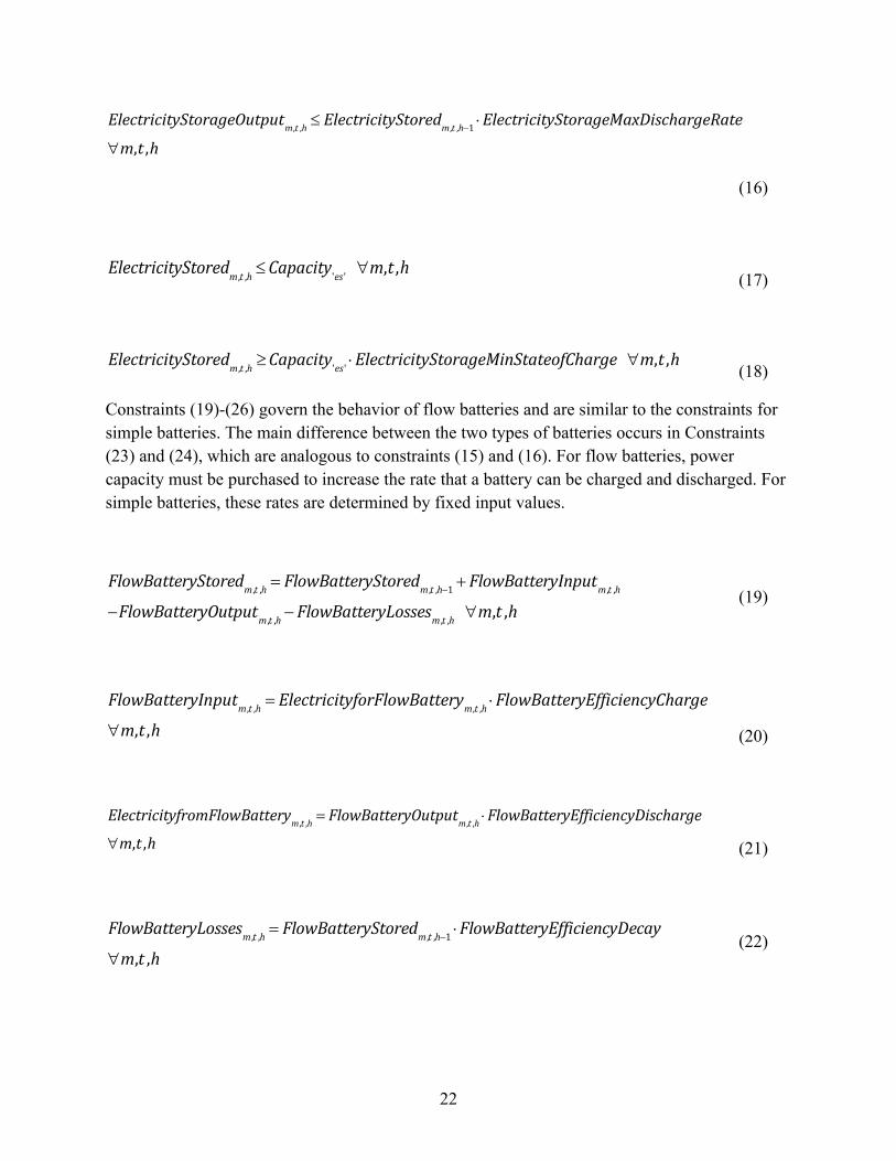
The first set of constraints is used to represent simple batteries. Constraint (11) is a continuity constraint that tracks the total amount of electricity stored in the batteries over the course of a day. Days are treated independently in order to reduce the computational complexity, so the continuity constraints do not enforce energy continuity across days. Constraints (12) and (13) account for energy losses due to charging and discharging inefficiencies, respectively. Constraint (14) accounts for the energy lost due to decay in the batteries. Constraints (15) and (16) limit the power input and output into and out of the battery, respectively. Constraints (17) and (18) ensure that the actual amount of energy in the batteries is within the appropriate upper and lower limits.
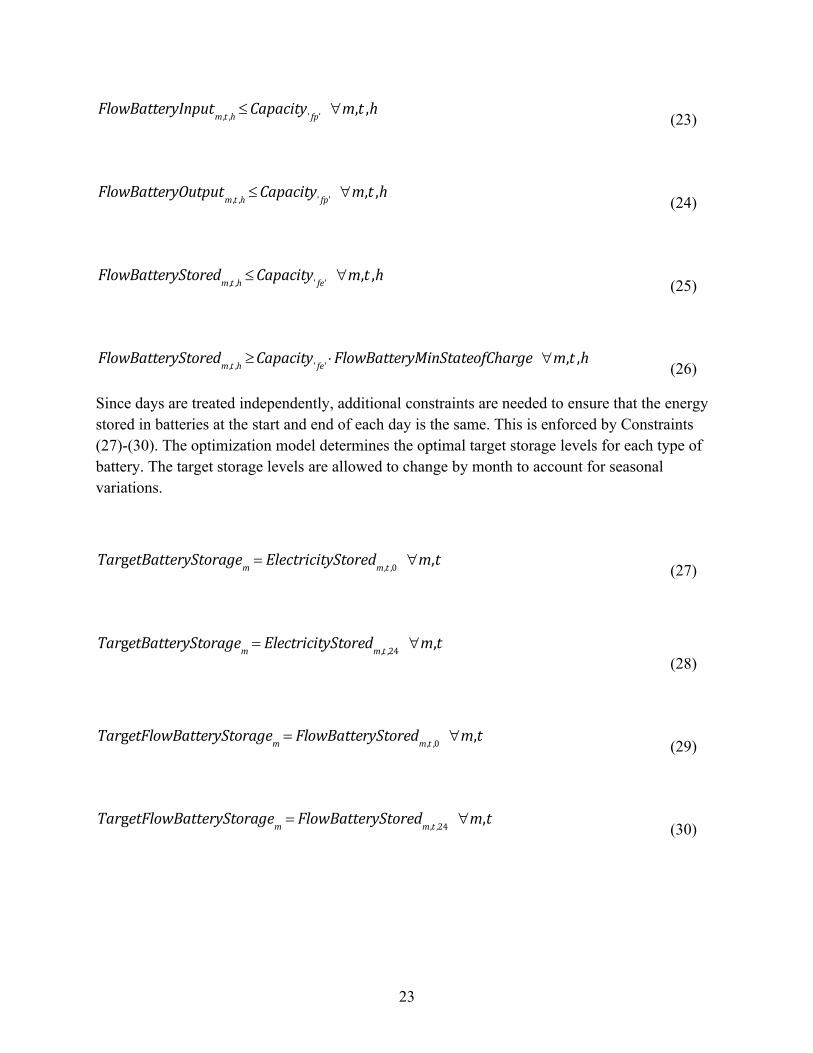
Constraints (19)-(26) govern the behavior of flow batteries and are similar to the constraints for simple batteries. The main difference between the two types of batteries occurs in Constraints (23) and (24), which are analogous to constraints (15) and (16). For flow batteries, power capacity must be purchased to increase the rate that a battery can be charged and discharged. For simple batteries, these rates are determined by fixed input values.
Since days are treated independently, additional constraints are needed to ensure that the energy stored in batteries at the start and end of each day is the same. This is enforced by Constraints (27)-(30). The optimization model determines the optimal target storage levels for each type of battery. The target storage levels are allowed to change by month to account for seasonal variations.
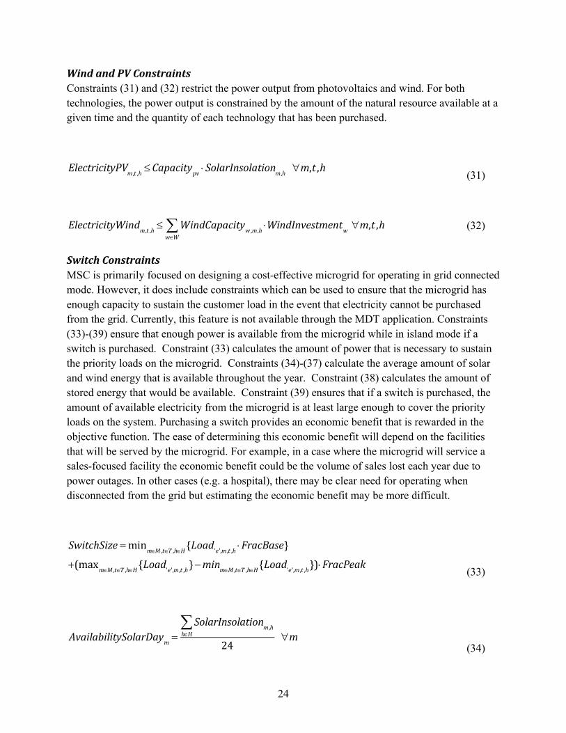
Wind and PV ConstraintsConstraints (31) and (32) restrict the power output from photovoltaics and wind. For both technologies, the power output is constrained by the amount of the natural resource available at a given time and the quantity of each technology that has been purchased.
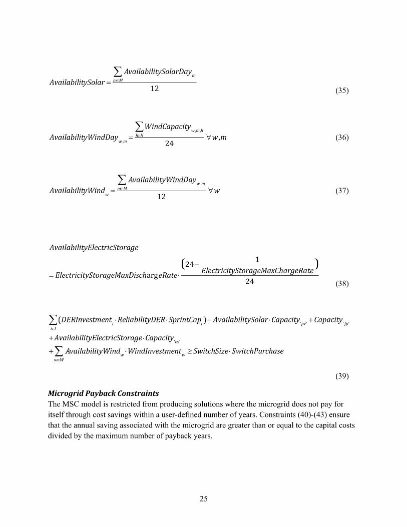
Switch ConstraintsMSC is primarily focused on designing a cost-effective microgrid for operating in grid connected mode. However, it does include constraints which can be used to ensure that the microgrid has enough capacity to sustain the customer load in the event that electricity cannot be purchased from the grid. Currently, this feature is not available through the MDT application. Constraints (33)-(39) ensure that enough power is available from the microgrid while in island mode if a switch is purchased. Constraint (33) calculates the amount of power that is necessary to sustain the priority loads on the microgrid. Constraints (34)-(37) calculate the average amount of solar and wind energy that is available throughout the year. Constraint (38) calculates the amount of stored energy that would be available. Constraint (39) ensures that if a switch is purchased, the amount of available electricity from the microgrid is at least large enough to cover the priority loads on the system. Purchasing a switch provides an economic benefit that is rewarded in the objective function. The ease of determining this economic benefit will depend on the facilities that will be served by the microgrid. For example, in a case where the microgrid will service a sales-focused facility the economic benefit could be the volume of sales lost each year due to power outages. In other cases (e.g. a hospital), there may be clear need for operating when disconnected from the grid but estimating the economic benefit may be more difficult.
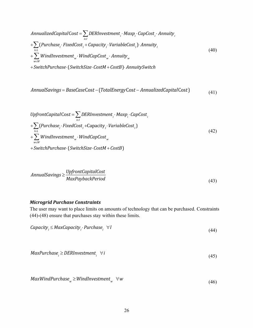
Microgrid Payback ConstraintsThe MSC model is restricted from producing solutions where the microgrid does not pay for itself through cost savings within a user-defined number of years. Constraints (40)-(43) ensure that the annual saving associated with the microgrid are greater than or equal to the capital costs divided by the maximum number of payback years.
26
AnnualizedCapitalCost DiI ERInvestment i Maxpi CapCost i Annuityi
(Purchasel FixedCost l Capacityl VariableCost l )lL Annuityl
UpfrontCapitalCost DiI ERInvestment i Maxpi CapCost i
(lL Purchasel FixedCost l Capacity l VariableCost l )
WwW indInvestmentw WindCapCostw
SwitchPurchase (SwitchSize CostM CostB)
(42)
AnnualSavings UpfrontCapitalCost
MaxPaybackPeriod (43)
Microgrid Purchase ConstraintsThe user may want to place limits on amounts of technology that can be purchased. Constraints (44)-(48) ensure that purchases stay within these limits.
Capacityl MaxCapacityl Purchasel l (44)
MaxPurchasei DERInvestmenti i (45)
MaxWindPurchasew WindInvestmentw w (46)
27
AllowPurchasel Purchasel l (47)
AllowSwitch SwitchPurchase (48)
Objective FunctionThe objective function includes all electricity market costs as well as the costs and savings associated with microgrid technologies. The electricity market costs include fees, demand, standby charges, electricity rates, and carbon taxes. Savings come from the use of a switch and electricity sold back to the grid. Costs associated with microgrid technologies include annual costs associated with fuel, operations and maintenance, as well as annualized upfront costs.
Minimize
TotalEnergyCost C
mM ontractDemandCharge maxmM ,tT ,hH {Load'e',m,t ,h }
M
mM onthlyFeeElectric
( (
iI
mM DERInvestment i Maxpi )Capacity'pv ' W
wW indInvestmentw Maxpw )StandbyCharge
Ehp
tT
pP
mM lectricityPurchasem,t ,h Nm,t ElectricityRatem,p
MdD
mM onthlyDemandRatesm,d maxtT ,hD{ElectricityPurchasem,t ,h }
DdD
tT
mM ailyDemandRatesm,d Nm,t maxhd {ElectricityPurchasem,t ,h }
2.3 Solution ProcedureThe MSC model is solved in two steps. The first step is to determine the base operating cost (BaseCaseCost) without a microgrid. MDT determines this by solving the model after setting the following parameters and variables to zero: BaseCaseCost, AnnualSaving, AllowPurchasel, MaxPurchasel, and MaxWindPurchasew. The value of the objective function from the first step (TotalEnergyCost) is used as the value of BaseCaseCost in a second run and the restrictions on AnnualSaving, AllowPurchasel, MaxPurchasel, and MaxWindPurchasew are removed.
29
3. TECHNOLOGY MANAGEMENT OPTIMIZATION (TMO)
TMO performs a multi-objective search to identify a collection of microgrid designs. The primary inputs to the model are a baseline microgrid design and a collection of design choices for the microgrid. The baseline design specifies the general structure of the microgrid but does not fully specify all choices that need to be made. The decision variables in the model are the design choices for elements of the microgrid. For example, a baseline design may specify that a generator is required in a specific building and the design choices for meeting this need could be a “500 kW Cummins Diesel” and an “800 kW Cat Diesel.” TMO treats the design choices as mutually exclusive. Therefore, its primary purpose is to figure out which choices to use to maximize satisfaction of the stated goals.
The multi-objective nature of TMO allows for multiple user goals to be considered simultaneously. This is important since there is likely not a single design that best meets all of the objectives. Given this, MDT is focused on seeking a collection of designs that together provide insights, trends, and trade-off information to support decision making and reduce the design space. As input, users can specify one or more goals to consider in an analysis. A goal consists of a quantitative metric of interest and an assertion about the desired values for that metric. The main assertions are its direction of improvement (maximize, minimize, or seek a particular value), the value that would be considered a minimally acceptable result (the limit), and the value that would be considered ideal (the objective). Limits can be violated though penalties will be incurred. To reduce the number of objectives considered during the optimization, metric level goals can be grouped. These groups are defined by the user and represent the major trade-off dimensions (cost, performance, reliability, etc.). The limit and objective information is used to normalize metric values so that they can be aggregated.
The optimization algorithm used in MDT searches the microgrid design space to find designs that best meet the defined objectives. The search space targeted by TMO is one of discrete categorical variables. In MDT, a microgrid design is created by selecting one of the valid design choices for each element of the baseline microgrid design. Once a design is identified, each of the relevant metrics can be calculated. In TMO, the metrics that are used to calculate the objective functions are unrestricted in form. Some metrics can be calculated using simple analytic functions. For example, a metric that focuses on purchase costs could be computed by adding the purchase cost for each element in the microgrid. For more complex calculations, TMO can access external models to determine metric values. MDT currently uses the PRM to quantify metrics related to the reliability and performance of a microgrid design in islanded mode.
TMO accesses an external solver to perform the optimization. The search algorithm used by TMO is a genetic algorithm (GA). A GA is a heuristic, population-based search technique that was inspired by ideas from evolutionary biology.2 This algorithm operates on a population of
30
individuals, where each individual represents a microgrid design. Each individual is represented by an array that identifies the design choice that is selected for each element of the microgrid. During each iteration of the algorithm, new solutions, referred to as children, are created by selecting and combining parents from the existing population. These child solutions inherit traits from the parent solutions. For each new solution, a fitness “score” is determined by calculating each of the metrics using PRM or a simple analytic function. In order to ensure that the size of the population does not grow too large, only subset of the solutions carry over to the next iteration of the algorithm. Those solutions that have a better fitness “score” (i.e. perform well with respect to one or more of the metrics compared to other solutions) are more likely to carry over to the next iteration of the algorithm. Additionally, the algorithm occasionally “mutates” individuals to introduce diversity into the population. An example of mutation would be randomly selecting an individual from the population and randomly changing the design choice for one of the microgrid elements. The GA mimics natural selection by creating new microgrid designs that inherit features from parent microgrid designs, randomly mutating features of designing, and favoring designs that have a higher fitness “score”.
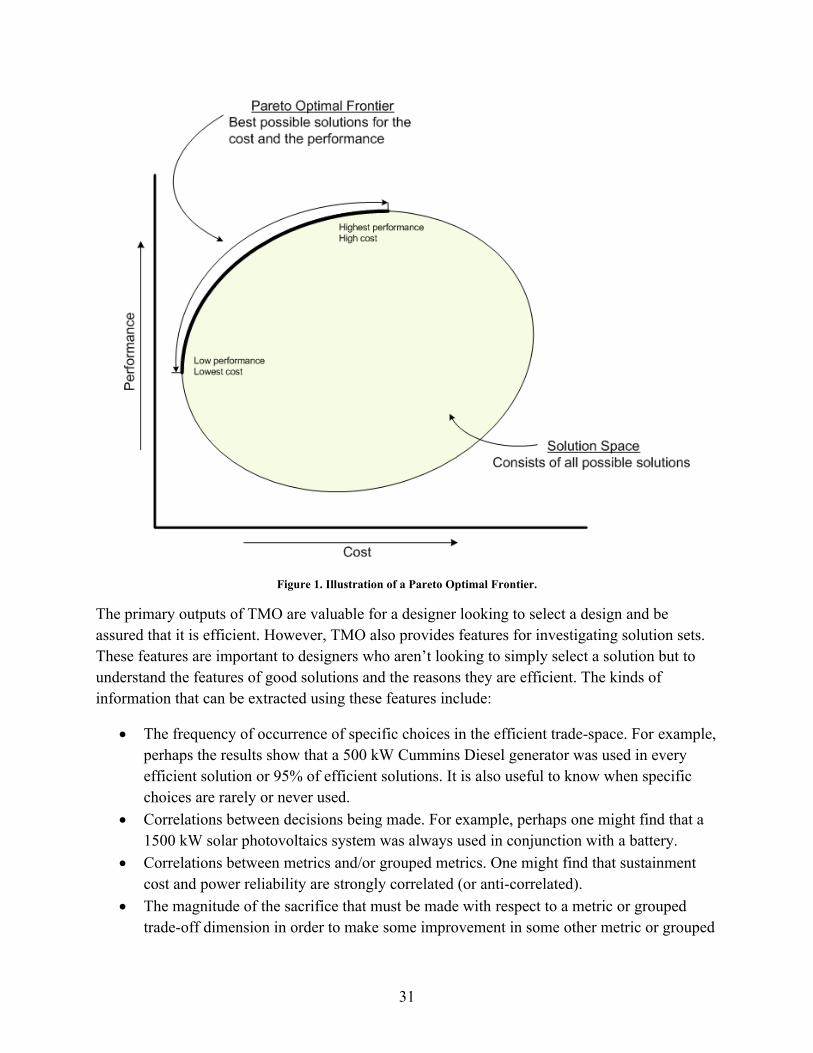
The primary output of TMO is a set of efficient trade-off microgrid designs, also referred to as a Pareto frontier. These designs have the quality that no other solution was found during the search that is better with respect to any one objective without being worse with respect to another objective. To understand this, consider a problem for which there are two groups of metrics: cost (comprised of cost related metrics) and performance (comprised of performance related metrics). Typically, the solution set will include points that have relatively high cost and high performance, low cost and low performance, and a range of options in between. Since the objective is to minimize cost and maximize performance, none of these solutions are inherently better or worse than any other solution. However, since these results show the trade-offs between solutions they can help decision makers identify solutions or characteristics of solutions that best meet their needs. This concept is illustrated in Figure 1. The solutions along the optimal frontier dominate all other solutions in the solution space.
2 Sait, Sadiq M., Youssef, Habib, “Iterative Computer Algorithms with Applications in Engineering: Solving Combinatorial Optimization Problems,” IEEE Computing Society, Los Alamitos, California, 1999, p. 109.
31
Figure 1. Illustration of a Pareto Optimal Frontier.
The primary outputs of TMO are valuable for a designer looking to select a design and be assured that it is efficient. However, TMO also provides features for investigating solution sets. These features are important to designers who aren’t looking to simply select a solution but to understand the features of good solutions and the reasons they are efficient. The kinds of information that can be extracted using these features include:
The frequency of occurrence of specific choices in the efficient trade-space. For example, perhaps the results show that a 500 kW Cummins Diesel generator was used in every efficient solution or 95% of efficient solutions. It is also useful to know when specific choices are rarely or never used.
Correlations between decisions being made. For example, perhaps one might find that a 1500 kW solar photovoltaics system was always used in conjunction with a battery.
Correlations between metrics and/or grouped metrics. One might find that sustainment cost and power reliability are strongly correlated (or anti-correlated).
The magnitude of the sacrifice that must be made with respect to a metric or grouped trade-off dimension in order to make some improvement in some other metric or grouped
32
dimension. For example, given some solution of interest, one could see how much it would cost to achieve a 5% increase in energy reliability.
Deeper analysis of design decision tradeoffs can be done by creating user-defined solutions, evaluating them using TMO, and plotting them alongside the solutions found by TMO. This feature can be used to figure out more of the “why” behind the trends and correlations seen in the output. For example, if a 1500 kW solar photovoltaics system was never used, defining a solution that forces this technology to be selected would show the impact of using this technology compared to the efficient solutions. This might indicate that certain critical goals cannot be satisfied or that the solution costs too much. This approach can also be used to evaluate microgrid designs that are not obtained through the MDT tool.
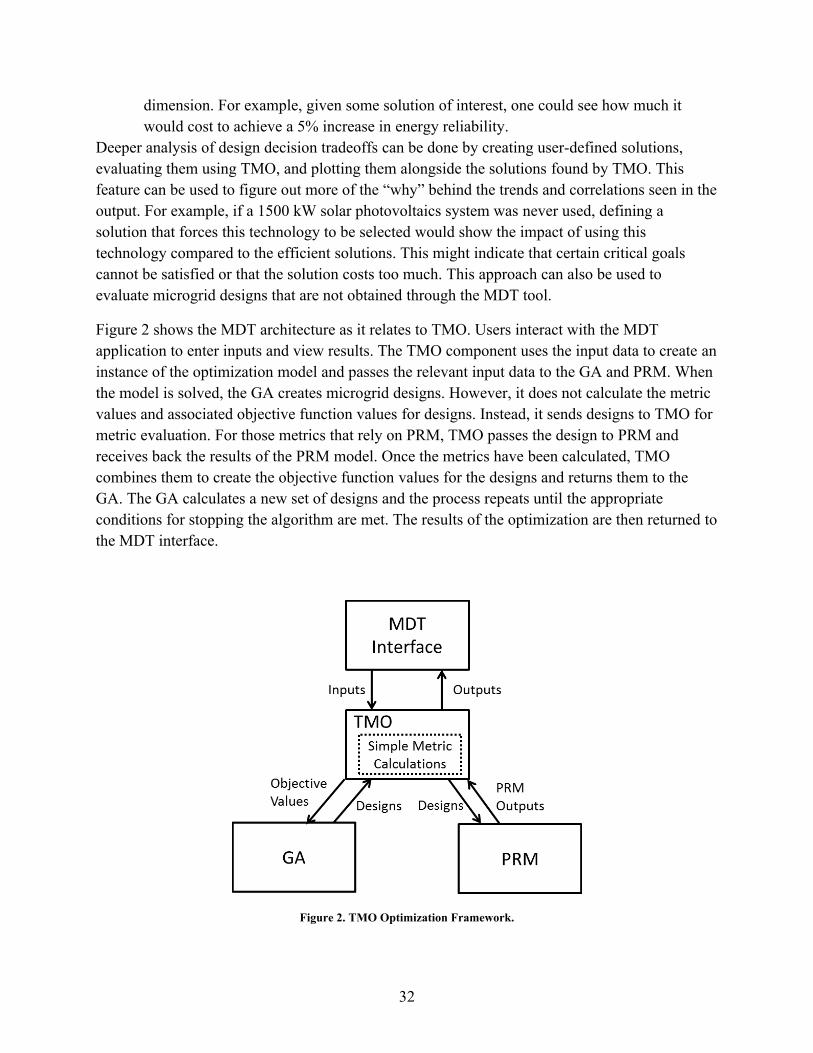
Figure 2 shows the MDT architecture as it relates to TMO. Users interact with the MDT application to enter inputs and view results. The TMO component uses the input data to create an instance of the optimization model and passes the relevant input data to the GA and PRM. When the model is solved, the GA creates microgrid designs. However, it does not calculate the metric values and associated objective function values for designs. Instead, it sends designs to TMO for metric evaluation. For those metrics that rely on PRM, TMO passes the design to PRM and receives back the results of the PRM model. Once the metrics have been calculated, TMO combines them to create the objective function values for the designs and returns them to the GA. The GA calculates a new set of designs and the process repeats until the appropriate conditions for stopping the algorithm are met. The results of the optimization are then returned to the MDT interface.
Figure 2. TMO Optimization Framework.
33
3.1 Model DescriptionThe subsections below describe the inputs to the model, the metrics that are calculated, the structure of the optimization, how it is solved, and the outputs that are returned to the analyst.
Model InputsAs shown in Figure 2, TMO receives the input data from the MDT interface. Some of this data is passed to PRM and used to calculate metrics that require PRM. This section primarily focuses on the data that is used to create microgrid designs and evaluate the metrics that do not require the use of PRM. See Section 4 for a detailed description of the inputs required by PRM.
For the purposes of performing the search for microgrid designs, the input data can be divided into two main groups: equipment specifications and baseline microgrid designs. Equipment specifications are collections of available equipment and technologies that can be used in microgrids. They are divided into groups such as diesel generators and transformers. The baseline microgrid describes the basic structure or topology of the microgrid. As the user defines the structure of the microgrid they also identify which equipment specifications can be used for each element of the system. When only a single specification is identified for an element, there is no decision to be made so the technology choice is fixed. When two or more specifications are identified there are options for how the microgrid should be designed. These become the model decision variables.
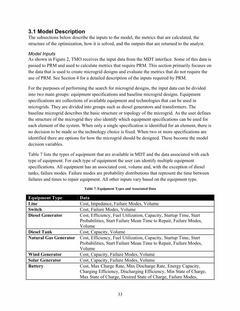
Table 7 lists the types of equipment that are available in MDT and the data associated with each type of equipment. For each type of equipment the user can identify multiple equipment specifications. All equipment has an associated cost, volume and, with the exception of diesel tanks, failure modes. Failure modes are probability distributions that represent the time between failures and times to repair equipment. All other inputs vary based on the equipment type.
Probabilities, Start Failure Mean Time to Repair, Failure Modes, Volume
Diesel Tank Cost, Capacity, VolumeNatural Gas Generator Cost, Efficiency, Fuel Utilization, Capacity, Startup Time, Start
Probabilities, Start Failure Mean Time to Repair, Failure Modes, Volume
Wind Generator Cost, Capacity, Failure Modes, VolumeSolar Generator Cost, Capacity, Failure Modes, VolumeBattery Cost, Max Charge Rate, Max Discharge Rate, Energy Capacity,
Charging Efficiency, Discharging Efficiency, Min State of Charge, Max State of Charge, Desired State of Charge, Failure Modes,
34
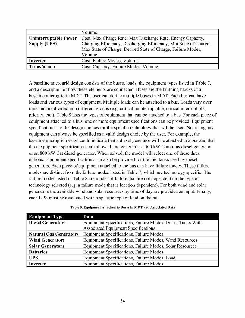
VolumeUninterruptable Power Supply (UPS)
Cost, Max Charge Rate, Max Discharge Rate, Energy Capacity, Charging Efficiency, Discharging Efficiency, Min State of Charge, Max State of Charge, Desired State of Charge, Failure Modes, Volume
A baseline microgrid design consists of the buses, loads, the equipment types listed in Table 7, and a description of how these elements are connected. Buses are the building blocks of a baseline microgrid in MDT. The user can define multiple buses in MDT. Each bus can have loads and various types of equipment. Multiple loads can be attached to a bus. Loads vary over time and are divided into different groups (e.g. critical uninterruptable, critical interruptible, priority, etc.). Table 8 lists the types of equipment that can be attached to a bus. For each piece of equipment attached to a bus, one or more equipment specifications can be provided. Equipment specifications are the design choices for the specific technology that will be used. Not using any equipment can always be specified as a valid design choice by the user. For example, the baseline microgrid design could indicate that a diesel generator will be attached to a bus and that three equipment specifications are allowed: no generator, a 500 kW Cummins diesel generator or an 800 kW Cat diesel generator. When solved, the model will select one of these three options. Equipment specifications can also be provided for the fuel tanks used by diesel generators. Each piece of equipment attached to the bus can have failure modes. These failure modes are distinct from the failure modes listed in Table 7, which are technology specific. The failure modes listed in Table 8 are modes of failure that are not dependent on the type of technology selected (e.g. a failure mode that is location dependent). For both wind and solar generators the available wind and solar resources by time of day are provided as input. Finally, each UPS must be associated with a specific type of load on the bus.
Table 8. Equipment Attached to Buses in MDT and Associated Data
Equipment Type DataDiesel Generators Equipment Specifications, Failure Modes, Diesel Tanks With
In addition to buses, the baseline microgrid design can contain transformers, switches, and nodes. Transformers have equipment specifications and failure modes. For each switch equipment specifications, failure modes and the default state (open or closed) can be specified. There is no input data associated with nodes. Nodes serve as points where lines can be connected.
Lines are the final input required when specifying a baseline microgrid design. Each line has a length, a set of line specifications that can be used, and failure modes. Choosing to not use a line is also a valid option. For each line, two endpoints must be specified. Any previously specified node, switch, transformer, bus, or element within a bus is a valid endpoint for a line.
Together these inputs specify the structure of the microgrid and the design choices that are available for each element of the microgrid. Recall that the elements in the baseline microgrid that have two or more equipment specification will be decision variables when the optimization is performed. In the MDT tool, the elements of a baseline microgrid design described above are referred to as “simple design elements.” This term is used because each of the equipment choices described so far can be made for each element without considering the choices made for other elements in the microgrid. In order to address cases where decisions cannot be made independently, MDT uses a concept called “complex design elements.” To illustrate this idea consider a case where two types of batteries and six types of photovoltaics are being considered at a particular bus. Using the simple design elements described above, there are twelve valid combinations of batteries and photovoltaic systems. However, compatibility issues may limit the number of valid combinations. Using complex design options, the user can specify which of the twelve combinations are valid. When solved, the optimization algorithm will not consider infeasible combinations of equipment.
Complex design elements can also be used to consider more complicated sets of decisions. Assume that there is a question about whether or not a building should be included in a microgrid. If it is not included, the baseline microgrid design can be used. However, if it is included in the microgrid, many additional elements will need to be included (buses, loads, generators, etc.). Furthermore, there may be options for the types of equipment that can be used for each new element. Using complex design elements the feasible configurations for this additional (and possibly optional) portion of the microgrid can be identified.
The inputs for complex design elements are essentially the same as for baseline microgrid. The user identifies the topology of the complex design element, which consists of a collection of simple elements (lines, buses, transformers, etc.), and the valid design choices for each of the simple elements. Only two additional inputs are required for complex design elements. First, the user can identify the combinations of design choices of simple elements that are not feasible. Second, the user can identify how the complex design element will be connected to the baseline microgrid design. For example, the complex design element may need to break an existing line
36
to be added to the baseline microgrid. The user can specify which line should be broken and where.
Model MetricsModel metrics are used to provide quantitative assessments of a microgrid design. They are also used to create the objective functions that are used in the multi-objective search. Table 9 provides a summary of the ten metrics currently used in MDT.
Table 9. Summary of MDT Metrics
Metric UnitsPurchase Cost DollarsMagnitude of Load not Served
kWh/Hour of Outage
Frequency of Load not Served
Percent of Utility Outages with Load not Served
Energy Availability %Diesel Fuel Used Gallons/Hour of OutageNatural Gas Used MBTU/Hour of OutageAverage Renewable Penetration
%
Diesel Efficiency %Natural Gas Efficiency %Volume Cubic Feet
All metrics have the same parameters: a limit, objective, improvement type, limit stiffness, and relative importance. The limit specifies the minimally acceptable metric value for a solution and the objective specifies the ideal value. Both of these inputs are in the units of the metric. The improvement type specifies whether the objective is to minimize, maximize, or seek a particular value for the metric. The limit stiffness specifies how strictly the limit value should be interpreted. It can be set to soft, medium, and hard. Finally, the relative importance is a non-negative real number that specifies how important a metric is compared to other metrics. All of these inputs are used to create the objective functions for the optimization algorithm.
The purchase cost and volume metrics are calculated by summing sum the purchase cost and volumes of all equipment used in the microgrid, respectively. All elements in the microgrid are included in these metrics, not just elements that have two or more design choices. All of the remaining metrics are calculated by the PRM model. See Section 4 for a detailed description of how these metrics are calculated.
Mathematical ModelThe mathematical model that TMO generates consists of three main parts: the choices to be made (decision variables), the constraints on the values of the decision variables, and the
37
objective functions that are used to evaluate solutions. The model has a decision variable for each of the design elements that have two or more equipment specifications. The value of a decision variable identifies the design choice that has been made for a given element and solution. A decision variable can represent a simple or complex design element. In the case of simple design elements, the value of the decision variable corresponds to a specific equipment selection. In the case of complex design elements, the value of the decision variable corresponds to a valid combination of equipment selections.
Let I be the number of design elements (simple or complex) that have two or more design options, and be an index on design elements. Let J(i) be the number of design choices that are available for design element i. The variable represents the equipment specification that is selected for design element i and x represents the vector of design choice variables. Constraint (50) states that each decision variable is restricted to the range of valid design choices. This implies that exactly one of the valid design choices must be selected for each design element.
(50)
Calculating the objective functions consist of three steps. First, the value for each metric is calculated for a given solution. Second, metric values must be converted to a normalized value so that they can be aggregated. Finally, the objective function values are calculated by aggregating the normalized metric values that are applicable to each objective function. Each metric can be mapped to at most one of the objective functions. Let N be the number of objective functions and be an index on the objective functions, and M(n) be the number of metrics that belong to objective function n. Let be the function that takes a solution x and converts it to a real valued number for the mth metric associated with objective function n. This function returns values that are in terms of the units of the metric. This function can be a simple analytic calculation (e.g. a sum of purchase costs) or represent the output of a model (i.e. PRM).
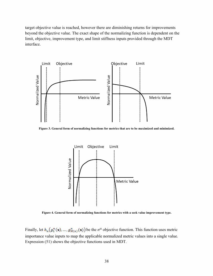
Each objective function in the model is created by combining a subset of the metrics into a single score. Since metrics can have different units, scales, and improvement directions (minimize, maximize or seek value), TMO uses normalizing functions to convert each metric to a normalized scale. Let be a function that converts metric into a normalized scale. It has the property that it increases as the target objective value is approached, therefore the final optimization problem can be written as a maximization problem. Figure 3 shows the general forms of the functions that are used to normalize metrics that are to be maximized and minimized. Figure 4 shows the general form of the function that is used to normalize metrics with a seek value improvement type. When the limit value is not met, the normalized value decreases at a large rate. This discourages solutions that do not meet the limit. Between the limit and objective metric values, the normalized score increases at a modest rate to reflect differences in solutions that are closer to the limit versus the target objective value. When the goal is to minimize or maximize a metric, the normalized objective value continues to increase after the
38
target objective value is reached, however there are diminishing returns for improvements beyond the objective value. The exact shape of the normalizing function is dependent on the limit, objective, improvement type, and limit stiffness inputs provided through the MDT interface.
Figure 3. General form of normalizing functions for metrics that are to be maximized and minimized.
Figure 4. General form of normalizing functions for metrics with a seek value improvement type.
Finally, let be the nth objective function. This function uses metric importance value inputs to map the applicable normalized metric values into a single value. Expression (51) shows the objective functions used in MDT.
39
(51)
Solution ProcedureThis section describes the key features of the GA that is used to solve the TMO optimization problem.
Gene RepresentationIn its most basic form, the gene used in the GA can be represented by the vector x, which has length I. The ith index of x corresponds to the ith design element and the value of the ith element of the array corresponds to the selected design choice. The value that the ith element of the array can take is restricted to one of the feasible design choices values, . Alternate representations of the gene (e.g. binary representations) can also be used to facilitate genetic operations.
This representation ensures that a valid design choice is selected for each element, which ensures that constraint (50) is not violated. Since the model does not contain any other constraints, feasible solutions can be constructed by selecting a valid design choice for each element.
InitializationThe initial population in the GA is generated by randomly selecting a design choice for each element for each individual. The size of the initial population is a parameter that can be modified by the user. The algorithm ensures that no two solutions in the initial population are identical.
CrossoverThe crossover algorithm used by the MDT is a multi-point, real value crossover routine. Crossover points are restricted to the locations between variables (elements of x). For each crossover operation, two crossover locations are identified randomly and two offspring designs are formed by selecting segments from two parents in accordance with the crossover locations. Figure 5 illustrates this crossover technique.
Figure 5. Illustrative example showing the crossover technique used in the MDT GA.
40
MutationThe mutation algorithm used by the MDT randomly changes design choices for a subset of the population. The algorithm uses a mutation rate parameter to determine the number of mutations that will occur. This parameter is not exposed to the user. For each mutation, the model randomly selects an individual from the full population. It then randomly selects an element of that individual and randomly selects a new design choice for that element. This process continues until the appropriate number of mutations has been performed. Individuals that are selected for mutation are eligible to be selected for subsequent mutations within an iteration of the GA.
Fitness Evaluation and Down-selectionThe fitness of individuals in the population is based on the degree to which each solution is dominated by other solutions. For each individual, the objective function values are used to determine the number of solutions that are dominant. Solutions that are on the efficient frontier will not be dominated by any solutions and will have the highest fitness score. Solutions that are dominated by a larger number of points are less fit. Only solutions that are dominated by a predefined number of solutions or fewer are carried over to the next iteration of the algorithm. This down-selection approach does not limit the size of the population.
Additional FeaturesThe GA contains several other features that improve the performance of the algorithm and the quality of the results. First, the GA does not allow multiple instances of a solution to be part of the population. This helps prevent the population from becoming homogeneous. Second, the algorithm includes several features to ensure that it terminates at a reasonable point in the solution process. The algorithm will terminate once it meets certain stopping criteria (e.g. wall clock time limit or a maximum number of iterations). It will also terminate when the efficient front of solutions converges. Three techniques are used to measure the convergence of the efficient frontier. The first technique measures change in location and shape of the frontier. The second technique measures changes in the density of the solutions on the frontier. The third technique measures changes in the solutions that form the boundary of the frontier. Changes in these metrics between successive intervals indicate that efficient frontier has not yet converged.
Model OutputsThe primary output of TMO is a set of efficient trade-off microgrid designs. These designs have the quality that no other solution was found during the search that is better with respect to any one objective function without being worse with respect to another. This result is useful for exploring the trade space of microgrid designs. For each solution, the microgrid design and associated metrics are also returned. The MDT tool provides a variety of methods for viewing and querying the collection of microgrid designs.
41
4. PERFORMANCE AND RELIABILITY MODEL
PRM is a discrete-event simulation which allows quantification of microgrid performance in terms of fuel efficiency, fuel usage, renewables penetration and usage, renewable spillage, dispatch statistics, and other operational metrics. Fuel costs are not currently considered, so fuel usage and efficiency reflect the demand and the efficiency of the dispatch algorithm. Microgrid reliability can be quantified in terms of frequency and magnitude of load lost on a tier-by-tier, load-by-load, or bus-by-bus basis, or on an aggregated basis over the microgrid. PRM also supports calculation and reporting of individual equipment reliability statistics.
As development and use of the model progresses, a future step could include creation of a library of OEM parameters that users could select from when defining the microgrid components.
PRM does not currently use an AC or DC optimal power flow, but incorporation of an AC optimal power flow model (AC-OPF) is a near term goal for the project.3 Instead, currently a microgrid dispatch algorithm within PRM uses rule sets to determine dispatch. Active dispatchable generation units, defined as those currently producing power and those already in the startup phase, are identified, and then a determination is made about adding or removing generation. Renewable energy sources are not considered dispatchable within PRM. PRM accepts a fixed amount of generation from renewable sources, and any excess is considered “spilled.”
Forecasted minimum, maximum, and average net effective load values are used as input to the dispatch logic. These forecasts are done over a user defined span of time. The current prediction model is a “noisy” version of actual load data. A net effective load value is the total load, but may be reduced by power coming from renewable generators.
The dispatch algorithm will start additional generators if:
There are fewer than the minimum allowable number running The maximum predicted load is greater than the maximum possible generation of the
currently running generators The maximum predicted load is greater than the reserve power requirement and the
average predicted load is closer to the maximum than the minimum.
The dispatch algorithm will stop running generators if:
3 Watson, Jean-Paul, Anya Castillo, Paula Lipka, Shmuel Oren and Richard O’Neill, “A Current-Voltage Successive Linear Programming Approach to Solving the ACOPF,” IEEE Transactions on Power Systems, 2010.
42
The minimum predicted load during the user defined period is less than the minimum generation value of the currently running set. (Minimum generation value is a parameter provided to the controller by the user.).
The average predicted load during the user defined period is closer to the minimum than the maximum.
The controller was unable to add any previously dropped loads, if they exist.
The dispatch algorithm will not violate the minimum allowable number of running generators. It also will not make changes to generation if the maximum predicted load is greater than the reserve requirement, but the average load is closer to the minimum than the maximum.
If there is insufficient generation to serve the load forecast,) such that a generator must be started, a list of non-active functional generators with enough fuel to run for the minimum runtime specified as a parameter to the dispatcher at the spinning reserve rate is created and then sorted by appropriateness for the load. This sorting is determined based on the maximum recommended running rate of each generator. The smallest generator capable of covering the predicted deficit is used, or if no available generator can cover the predicted deficit then larger generators are chosen. The selected generator is then scheduled for start. Once it enters its startup procedure, the deficit is reduced by the selected generator’s recommended maximum rate, and the remaining list is resorted using the new predicted shortfall in generation.
If there is predicted excess generation, all currently active generators for which a shutdown would not result in shedding more than the excess generation are identified and a sort is performed based on the recommended running rate of the generators (kW). The largest generator from that list is scheduled for shutdown. The process is repeated until the required minimum number of running generators has been reached, the predicted excess power is gone or there are no more generators that can be shut down without resulting in a deficit.The full set of power sources considered are solar power, wind power, fossil generators, and storage assets, including UPSs. The simulation only draws from storage assets if a generation deficit remains after exhausting other alternatives, and batteries are drained before UPSs.
If there is excess power remaining and generators are not shut down by the dispatching logic, the excess power may be used to charge UPSs and batteries. Once the amounts coming from solar and wind are accounted, the rest must be covered by the fossil generators and then if necessary, storage assets (batteries and UPSs). The fossil fuel generators are all assumed to run at the same level of output. That utilization is defined by the amount of power needed divided by the total fossil fuel generation capacity. If there is not adequate generation to meet the total load after all generation alternatives are in use, loads are dropped if possible. A load can only be dropped if a switch exists in the path between that load and the bus. The logic for dropping loads is similar to the logic for starting and stopping generators, in that a list of droppable loads is created and
43
sorted by appropriateness, which is a function of user defined load criticality category (referred to as a tier) followed by priority followed by size. Loads are dropped one at a time until enough load has been removed.
Once all utilization rates are determined, events are added to the queue to reflect limits on operation. For example, if a generator running at the specified rate will run out of fuel before the next event or a battery will reach its minimum state of charge, events will be generated to reflect that in the simulation.
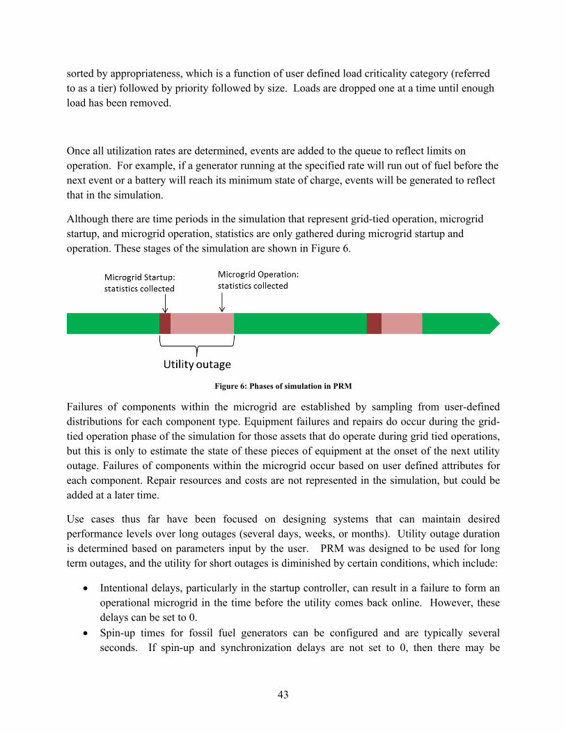
Although there are time periods in the simulation that represent grid-tied operation, microgrid startup, and microgrid operation, statistics are only gathered during microgrid startup and operation. These stages of the simulation are shown in Figure 6.
Figure 6: Phases of simulation in PRM
Failures of components within the microgrid are established by sampling from user-defined distributions for each component type. Equipment failures and repairs do occur during the grid-tied operation phase of the simulation for those assets that do operate during grid tied operations, but this is only to estimate the state of these pieces of equipment at the onset of the next utility outage. Failures of components within the microgrid occur based on user defined attributes for each component. Repair resources and costs are not represented in the simulation, but could be added at a later time.
Use cases thus far have been focused on designing systems that can maintain desired performance levels over long outages (several days, weeks, or months). Utility outage duration is determined based on parameters input by the user. PRM was designed to be used for long term outages, and the utility for short outages is diminished by certain conditions, which include:
Intentional delays, particularly in the startup controller, can result in a failure to form an operational microgrid in the time before the utility comes back online. However, these delays can be set to 0.
Spin-up times for fossil fuel generators can be configured and are typically several seconds. If spin-up and synchronization delays are not set to 0, then there may be
44
inadequate time to get the emergency generators online before the utility power returns. Only UPS protected loads will be served in such a case.
The “long outage” paradigm is the one for which the PRM has been most heavily tested and used. The PRM is written in C++, depends on the C++11 standard, and leverages several of the Boost C++ libraries (www.boost.org). It can be used in stand-alone mode, but that mode requires a programmer to enter input data. The intended use is “library mode,” in which information can be provided via the Application Programming Interface (API).
Model InputsThe primary input to the PRM is a microgrid topology specification. The topology specification includes elements such as electrical lines, buses, switches, and transformers. Component characteristics such as sizes, lengths, electrical properties, and capacities must also be specified.
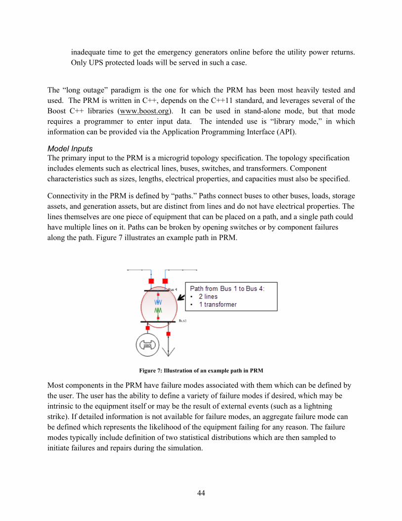
Connectivity in the PRM is defined by “paths.” Paths connect buses to other buses, loads, storage assets, and generation assets, but are distinct from lines and do not have electrical properties. The lines themselves are one piece of equipment that can be placed on a path, and a single path could have multiple lines on it. Paths can be broken by opening switches or by component failures along the path. Figure 7 illustrates an example path in PRM.
Figure 7: Illustration of an example path in PRM
Most components in the PRM have failure modes associated with them which can be defined by the user. The user has the ability to define a variety of failure modes if desired, which may be intrinsic to the equipment itself or may be the result of external events (such as a lightning strike). If detailed information is not available for failure modes, an aggregate failure mode can be defined which represents the likelihood of the equipment failing for any reason. The failure modes typically include definition of two statistical distributions which are then sampled to initiate failures and repairs during the simulation.
Operational parameters of the microgrid are also defined by the user. These values are used by the simulation to execute logic for each phase of microgrid operation. PRM also has several configuration settings that allow for customization of the simulation behavior.
The following list details all of the input values that can be defined by the user. For more information on how these inputs are used and to ensure the most up to date list of inputs, see the Microgrid Design Toolkit User Guide.
Site:1. Label2. List of Grids3. Power Utility Information
Power Utility:1. Label2. Reliability Data
For each Grid:1. Label2. List of buses3. Choice of startup controller + Parameters4. Choice of microgrid controller + Parameters5. Choice of grid tied controller + Parameters6. Choice of refueling strategy (if applicable) + Parameters7. Choice of generator dispatcher + Parameters8. List of electrical paths9. Statistics Configuration Information
For the Startup Controller:1. Generator Restart Attempt Delay2. Generator Synchronization Delay3. Bus Synchronization Delay4. Microgrid Formation Delay – No Generator Failures5. Microgrid Formation Delay – Generator Failures6. Renewable Close-in Delay
For each Bus:1. Label2. Solar Generator output Data (normalized time series data)3. Wind Generator output Data (normalized time series data)4. Choice of fuel manager (handles feeding generators from fuel tanks).5. Priority6. List of Load Sections7. List of UPSs8. List of Batteries9. List of Wind Generators10. List of Solar Generators11. List of Diesel Generators12. List of Diesel Tanks13. List of Natural Gas Generators14. Statistics Configuration Information
For each Load Section:1. Label2. Actual Load Data (time series data, 1 column for each tier)3. Predicted Load Data (time series data, 1 column for each tier)4. Priority
For each UPS:1. Label2. Capacity3. Maximum Charge Rate4. Maximum Discharge Rate5. Minimum Allowable State of Charge6. Maximum Allowable State of Charge7. Initial State of Charge8. Desired State of Charge9. Charging efficiency10. Discharging efficiency11. Reliability Data12. Statistics Configuration Information
For each Battery:1. Label2. Capacity3. Maximum Charge Rate4. Maximum Discharge Rate5. Minimum Allowable State of Charge6. Maximum Allowable State of Charge7. Initial State of Charge8. Desired State of Charge 9. Charging efficiency
47
10. Discharging efficiency11. Reliability Data12. Statistics Configuration Information
For each Wind Generator:1. Label2. Capacity 3. Wind Generator output Data (normalized time series data)4. Reliability Data5. Statistics Configuration Information
For each Solar Generator: 1. Label2. Capacity 3. Wind Generator output Data (normalized time series data)4. Reliability Data5. Statistics Configuration Information
For each Diesel Generator: 1. Label2. Capacity3. Spinning Reserve Rate4. Startup Probability Vector5. Microgrid Enabled Status6. Minimum Allowable Utilization Rate7. Minimum Runtime8. Minimum Cool Time9. Startup Power Output Profile10. Fuel Utilization Profile11. Efficiency Profile12. Reliability Data13. Statistics Configuration Information
For each Diesel Tank:1. Label2. Capacity3. Initial Quantity4. List of Attached Diesel Generators5. Statistics Configuration Information
For each Natural Gas Generator: 1. Label2. Capacity3. Spinning Reserve Rate4. Startup Probability Vector5. Microgrid Enabled Status
For each Bus-Bus Path:1. Path Information2. 1st Connected Bus3. 2nd Connected Bus
For each Bus-Asset Path: 1. Path Information2. Connected Bus3. Connected Asset4. Contained Inverter (if one)
For each Bus-Load Path: 1. Path Information2. Connected Bus3. Connected Load Section4. List of UPSs
For each Path:1. Label2. Priority3. List of Lines4. List of Transformers5. List of Switches
For each Line:1. Capacity in Direction 12. Capacity in Direction 23. Reliability Data4. Statistics Configuration Information
For each Transformer:1. Capacity 2. Reliability Data3. Statistics Configuration Information
For each Switch:1. Initial Open State
49
For each Inverter: 2. Label3. Initial Connection State4. Ability to Maintain Connection through Onset of Utility Outage.5. Reliability Data
Power Output Profile:1. List of pairs of [time, output %] from ignition to max power output %
Reliability Data:1. List of Failure Modes
For each Failure Mode:1. Label2. Choice of Failure Event Generator (callable object typically backed by a distribution)3. Choice of Repair Event Generator (callable object typically backed by a distribution)
Fuel Utilization Profile (UOM = Unit of Measure):1. 25% Capacity Fuel Utilization Value (Fuel UOM/Capacity UOM/hour)2. 50% Capacity Fuel Utilization Value (Fuel UOM/Capacity UOM/hour)3. 75% Capacity Fuel Utilization Value (Fuel UOM/Capacity UOM/hour)4. 100% Capacity Fuel Utilization Value (Fuel UOM/Capacity UOM/hour)
Efficiency Profile:1. 25% Capacity Efficiency Value (%)2. 50% Capacity Efficiency Value (%)3. 75% Capacity Efficiency Value (%)4. 100% Capacity Efficiency Value (%)
Grid Statistics Configuration Information:1. Renewable penetration histogram bin upper bounds
Bus Statistics Configuration Information:None
UPS Statistics Configuration Information:1. State of charge histogram bin upper bounds
Battery Statistics Configuration Information:1. State of charge histogram bin upper bounds
Natural Gas Generator Statistics Configuration Information:1. Utilization rate histogram bin upper bounds
Line Statistics Configuration Information: 1. Overload histogram bin upper bounds
Model OutputsOutputs are available in PRM which provide statistics for categories such as reliability, batteries, loads, buses, generators, diesel tanks, and renewable generation.
The following sections detail all of the output values that are available to the user.
Reliability StatisticsRaw Statistics:
Min, Max, Count, Sum, and Mean of downtime durations Min, Max, Count, Sum, and Mean of operational durations Min, Max, Count, Sum, and Mean of all downtime attributable to each failure
modeAvailable Computed Values:
None
Battery StatisticsRaw Statistics:
All Reliability Statistics Min, Max, Count, Sum, Mean, and Variance of runtime Min, Max, Count, Weighted Sum, Weighted Mean, Sum of Weights, and 2nd
Weighted Moment of power (weights – time) Min, Max, Count, Weighted Sum, Weighted Mean, Sum of Weights, and 2nd
Weighted Moment of state of charge (weights – time) Time Histogram of State of Charge (bins are definable)
Available Computed Values:
Variance of power Variance of State of Charge
51
Load StatisticsRaw Statistics:
Min, Max, Count, Sum, and Mean of total load served for each tier. Min, Max, Count, Sum, and Mean of total load not served for each tier. Min, Max, Count, Sum, and Mean of post-startup load served for each tier. Min, Max, Count, Sum, and Mean of post-startup load not served for each tier. Min, Max, Count, Sum, and Mean of load not served for each tier accounted only
for those utility outages for which any tier load not served was observed.Available Computed Values:
Overall Energy Availability for each tier (%) Post-Startup Energy Availability for each tier (%)
Bus StatisticsRaw Statistics:
All Load StatisticsAvailable Computed Values:
All Available Computed Values of Load Statistics
Capacity Limitation Statistics (not currently used)Raw Statistics:
Min, Max, Count, Weighted Sum, Weighted Mean, Sum of Weights, and 2nd Weighted Moment of overloads (weights – time)
Time histogram of overloads (bins are definable)Available Computed Values:
Variance of overloads
Generator StatisticsRaw Statistics:
Min, Max, Count, Sum, Mean, and Variance of % utilization Min, Max, Count, Sum, Mean, and Variance of efficiency Min, Max, Count, Sum, Mean, and Variance of runtime Min, Max, Count, Sum, Mean, and Variance of offline time Min, Max, Count, Sum, Mean, and Variance of total energy produced Time Histogram of % Utilization (bins are definable)
Available Computed Values:
52
Standard Deviation of % utilization Standard Deviation of efficiency Standard Deviation of energy produced Standard Deviation of runtime Standard Deviation of offline time
Fuel-Based Generator StatisticsRaw Statistics:
All Generator Statistics All Reliability Statistics Min, Max, Count, Sum, and Mean of fuel used during a utility outage
Available Computed Values:
All Available Computed Values of Generator Statistics All Available Computed Values of Reliability Statistics
Diesel Generator StatisticsRaw Statistics:
All Fuel-Based Generator StatisticsAvailable Computed Values:
All Available Computed Values of Fuel-Based Generator Statistics
Diesel Tank StatisticsRaw Statistics:
Min, Max, Count, Sum, Mean, and Variance of fuel used during a utility outage Time Histogram of fuel level (bins are definable)
Available Computed Values:
Standard Deviation of fuel used during a utility outage
Grid StatisticsRaw Statistics:
All Load Statistics
53
Count, Sum, and Mean of number of fuel based generator dispatch calls (used in the logic that decides whether or not to start or stop fuel based generators)
Count, Sum, and Mean of number of times entry in the fuel based generator dispatch logic resulted in a change to the set of running generators
Min, Max, Count, Sum, and Mean of the diesel fuel used during utility outages Min, Max, Count, Sum, and Mean of the natural gas used during utility outages Min, Max, Count, Sum, and Mean of the solar power generated during utility
outages Min, Max, Count, Sum, and Mean of the solar power spilled during utility outages Min, Max, Count, Sum, and Mean of the wind power generated during utility
outages Min, Max, Count, Sum, and Mean of the wind power spilled during utility
outages Min, Max, Count, Weighted Sum, Weighted Mean, Sum of Weights, and 2nd
Weighted Moment of renewable penetration (penetration %, weights – time) Time Histogram of renewable penetration (penetrations %, bins are definable)
Available Computed Values:
All Available Computed Values of Load Statistics Variance of renewable penetration
Load Section StatisticsRaw Statistics:
All Load Statistics
Available Computed Values:
All Available Computed Values of Load Statistics
Natural Gas Generator StatisticsRaw Statistics:
All Fuel-Based Generator StatisticsAvailable Computed Values:
All Available Computed Values of Fuel-Based Generator Statistics
54
Renewable Generator StatisticsRaw Statistics:
All Generator Statistics All Reliability Statistics Min, Max, Count, Sum, Mean, and Variance of energy spilled during a utility
outage
Available Computed Values:
All Available Computed Values of Generator Statistics All Available Computed Values of Reliability Statistics Standard Deviation of energy spilled during a utility outage
Site StatisticsRaw Statistics:
All Load Statistics Min, Max, Count, Sum, and Mean of the diesel fuel used during utility outages Min, Max, Count, Sum, and Mean of the natural gas used during utility outages Min, Max, Count, Sum, and Mean of the solar power generated during utility
outages Min, Max, Count, Sum, and Mean of the solar power spilled during utility outages Min, Max, Count, Sum, and Mean of the wind power generated during utility
outages Min, Max, Count, Sum, and Mean of the wind power spilled during utility
outages Min, Max, Count, Weighted Sum, Weighted Mean, Sum of Weights, and 2nd
Weighted Moment of renewable penetration (penetration %, weights – time) Time Histogram of renewable penetration (penetration in %, bins are definable)
Available Computed Values:
All Available Computed Values of Load Statistics Variance of Renewable Penetration
Solar Generator, Wind Generator, and Inverter StatisticsRaw Statistics:
All Renewable Generator Statistics
55
Available Computed Values:
All Available Computed Values of Renewable Generator Statistics
Line StatisticsRaw Statistics:
All Reliability Statistics All Capacity Limitation Statistics
Available Computed Values:
All Available Computed Values of Reliability Statistics All Available Computed Values of Capacity Limitation Statistics
Power Utility StatisticsRaw Statistics:
All Reliability Statistics
Available Computed Values:
All Available Computed Values of Reliability Statistics
Switch StatisticsRaw Statistics:
All Reliability Statistics
Available Computed Values:
All Available Computed Values of Reliability Statistics
Transformer StatisticsRaw Statistics:
All Reliability Statistics All Capacity Limitation Statistics
56
Available Computed Values:
All Available Computed Values of Reliability Statistics All Available Computed Values of Capacity Limitation Statistics
UPS StatisticsRaw Statistics:
All Battery Statistics
Available Computed Values:
All Available Computed Values of Battery Statistics
Computed Values by Result Set based on Statistics Average Diesel Generator Efficiency on the Site – All Generators Average Diesel Generator Efficiency on the Site – Microgrid Enabled Generators
Only Average Diesel Generator Efficiency on the Site – Non-Microgrid Enabled
Generators Only Average Natural Gas Generator Efficiency on the Site – All Generators Average Natural Gas Generator Efficiency on the Site – Microgrid Enabled
Generators Only Average Natural Gas Generator Efficiency on the Site – Non-Microgrid Enabled
Generators Only Average Fuel-Based Generator Efficiency on the Site – All Generators Average Fuel-Based Generator Efficiency on the Site – Microgrid Enabled
Generators Only Average Fuel-Based Generator Efficiency on the Site – Non-Microgrid Enabled
Generators Only Average Diesel Generator Efficiency on a Specified Microgrid – All Generators Average Diesel Generator Efficiency on a Specified Microgrid – Microgrid
Enabled Generators Only Average Diesel Generator Efficiency on a Specified Microgrid – Non-Microgrid
Enabled Generators Only Average Natural Gas Generator Efficiency on a Specified Microgrid – All
Generators Average Natural Gas Generator Efficiency on a Specified Microgrid – Microgrid
Enabled Generators Only
57
Average Natural Gas Generator Efficiency on a Specified Microgrid – Non-Microgrid Enabled Generators Only
Average Fuel-Based Generator Efficiency on a Specified Microgrid – All Generators
Average Fuel-Based Generator Efficiency on a Specified Microgrid – Microgrid Enabled Generators Only
Average Fuel-Based Generator Efficiency on a Specified Microgrid – Non-Microgrid Enabled Generators Only
Average Diesel Generator Efficiency on a Specified Bus – All Generators Average Diesel Generator Efficiency on a Specified Bus – Microgrid Enabled
Generators Only Average Diesel Generator Efficiency on a Specified Bus – Non-Microgrid
Enabled Generators Only Average Natural Gas Generator Efficiency on a Specified Bus – All Generators Average Natural Gas Generator Efficiency on a Specified Bus – Microgrid
Enabled Generators Only Average Natural Gas Generator Efficiency on a Specified Bus – Non-Microgrid
Enabled Generators Only Average Fuel-Based Generator Efficiency on a Specified Bus – All Generators Average Fuel-Based Generator Efficiency on a Specified Bus – Microgrid
Enabled Generators Only Average Fuel-Based Generator Efficiency on a Specified Bus – Non-Microgrid
Enabled Generators Only Total Solar Energy Generated on the Site Total Wind Energy Generated on the Site Total Renewable Energy Generated on the Site Total Solar Energy Generated on a Specified Microgrid Total Wind Energy Generated on a Specified Microgrid Total Renewable Energy Generated on a Specified Microgrid Total Solar Energy Generated on a Specified Bus Total Wind Energy Generated on a Specified Bus Total Renewable Energy Generated on a Specified Bus
58
59
5. CONCLUSIONS
This document summarizes the two capabilities currently implemented in MDT. MSC provides an initial sizing capability that can be used in the early stages of designing a microgrid. The capability comprised of TMO and PRM can be used to refine microgrid designs in later stages of the design process. Future development for this capability could fall into three main areas. The first area would be adding additional capabilities to help analysts in the design steps between MSC and TMO/PRM. For example, algorithms could be developed and added to the MDT tool to assist with developing network topologies. Second, the existing capabilities could be updated to include more detailed representations of power flow. Finally, algorithms could be developed and added to the MDT that would connect the various capabilities in the tool. This would allow outputs from one capability to be converted to inputs for other capabilities in an automated fashion.
60
61
6. REFERENCES
1. Stadler, Michael, Chris Marnay, Afzal S. Siddiqui, Judy Lai, Brian Coffey, and Hirohisa Aki, “Effect of Heat and Electricity Storage and Reliability on Microgrid Viability: A Study of Commercial Buildings in California and New York States,” LBNL-1334E, 2008, available at https://building-microgrid.lbl.gov/publications/effect-heat-and-electricity-storage, accessed June 24, 2015.
2. Sait, Sadiq M., Youssef, Habib, “Iterative Computer Algorithms with Applications in Engineering: Solving Combinatorial Optimization Problems,” IEEE Computing Society, Los Alamitos, California, 1999, p. 109.
3. Watson, Jean-Paul, Anya Castillo, Paula Lipka, Shmuel Oren and Richard O’Neill, “A Current-Voltage Successive Linear Programming Approach to Solving the ACOPF,” IEEE Transactions on Power Systems, 2010.