48
Microsoft Excel 2013 Chapter 2 Formulas, Functions, and Formatting
| Date post: | 07-Feb-2018 |
| Category: |
Documents |
| Upload: | trinhduong |
| View: | 221 times |
| Download: | 0 times |

Microsoft
Excel 2013
Chapter 2
Formulas, Functions,and Formatting

• Enter formulas using the keyboard
• Enter formulas using Point mode
• Apply the MAX, MIN, and AVERAGE functions
• Verify a formula using Range Finder
• Apply a theme to a workbook
• Apply a date format to a cell or range
Objectives
Formulas, Functions, and Formatting 2

• Add conditional formatting to cells
• Change column width and row height
• Check the spelling on a worksheet
• Change margins and headers in Page Layout view
• Preview and print versions and sections of a worksheet
Formulas, Functions, and Formatting 3
Objectives

Formulas, Functions, and Formatting 4
Project – Worksheet with Formulas and
Functions

• Enter formulas in the worksheet
• Enter functions in the worksheet
• Verify formulas in the worksheet
• Format the worksheet
• Check spelling
• Print the worksheet
Formulas, Functions, and Formatting 5
Roadmap

Formulas, Functions, and Formatting 6
Entering a Formula Using the Keyboard
• With the cell to contain the formula selected, type the formula in the cell to display the formula in the formula bar and in the current cell and to display colored borders around the cells referenced in the formula
• Press the right arrow key to complete the arithmetic operation indicated by the formula, to display the result in the worksheet, and to select the cell to the right

Formulas, Functions, and Formatting 7
Entering a Formula Using the Keyboard

Formulas, Functions, and Formatting 8
Arithmetic Operations

Formulas, Functions, and Formatting 9
Order of Operations

Formulas, Functions, and Formatting 10
Entering Formulas Using Point Mode
• With the cell that is to contain the formula selected, begin typing the formula and then tap or click another cell to add a cell reference in the formula
• Finish typing the rest of the formula• Tap or click the Enter box in the formula bar
when you have finished entering the formula

Formulas, Functions, and Formatting 11
Entering Formulas Using Point Mode
Formulas, Functions, and Formatting 12
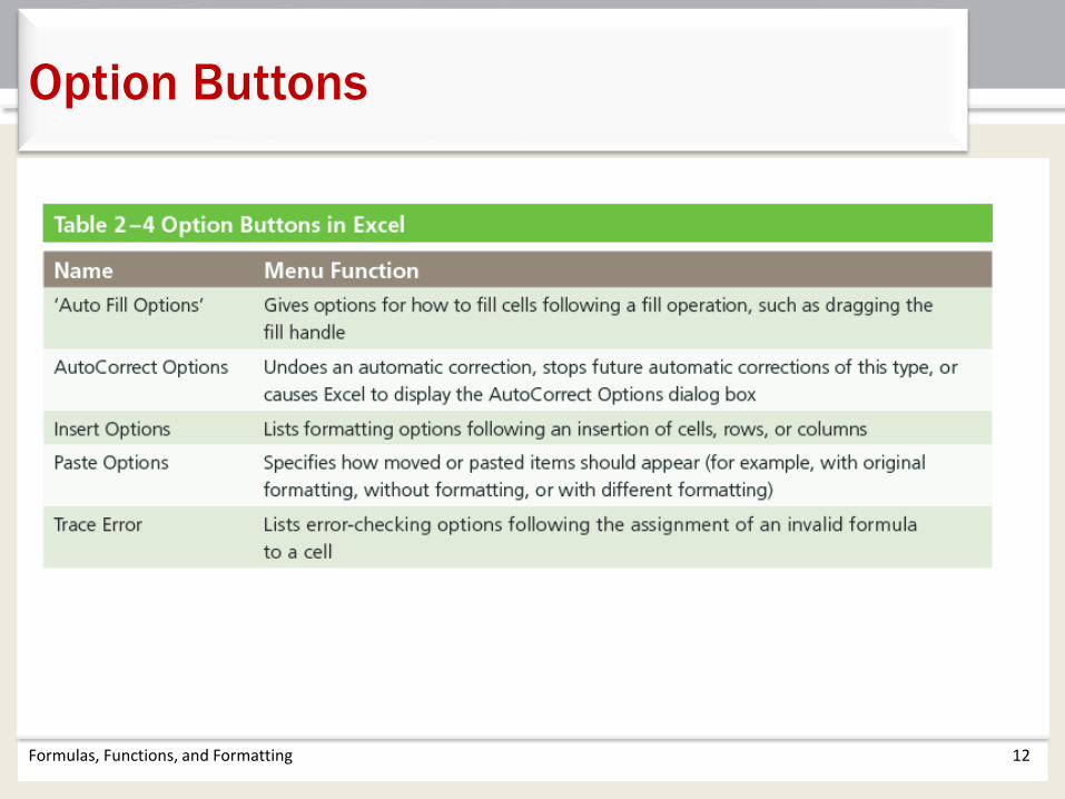
Option Buttons

Formulas, Functions, and Formatting 13
Determining the Highest Number in a Range
of Numbers Using the Insert Function Box
• Select the cell to contain the maximum number• Tap or click the Insert Function box in the formula bar
to display the Insert Function dialog box• If necessary, scroll to and then tap or click MAX in the
Select a function list • Tap or click the OK button to display the Function
Arguments dialog box and type the cell range in the Number1 box to enter the first argument of the function
• Tap or click the OK button to display the highest value in the chosen range in the selected cell

Formulas, Functions, and Formatting 14
Determining the Highest Number in a Range
of Numbers Using the Insert Function Box
Formulas, Functions, and Formatting 15
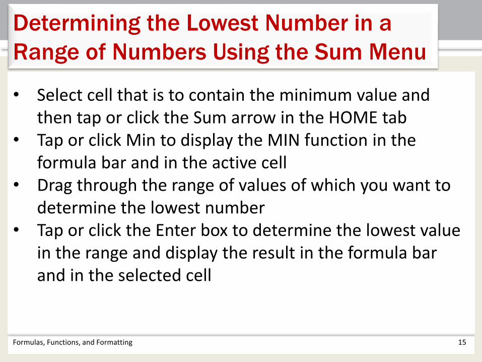
Determining the Lowest Number in a
Range of Numbers Using the Sum Menu
• Select cell that is to contain the minimum value and then tap or click the Sum arrow in the HOME tab
• Tap or click Min to display the MIN function in the formula bar and in the active cell
• Drag through the range of values of which you want to determine the lowest number
• Tap or click the Enter box to determine the lowest value in the range and display the result in the formula bar and in the selected cell
Formulas, Functions, and Formatting 16
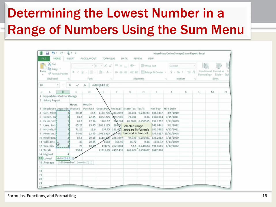
Determining the Lowest Number in a
Range of Numbers Using the Sum Menu

Formulas, Functions, and Formatting 17
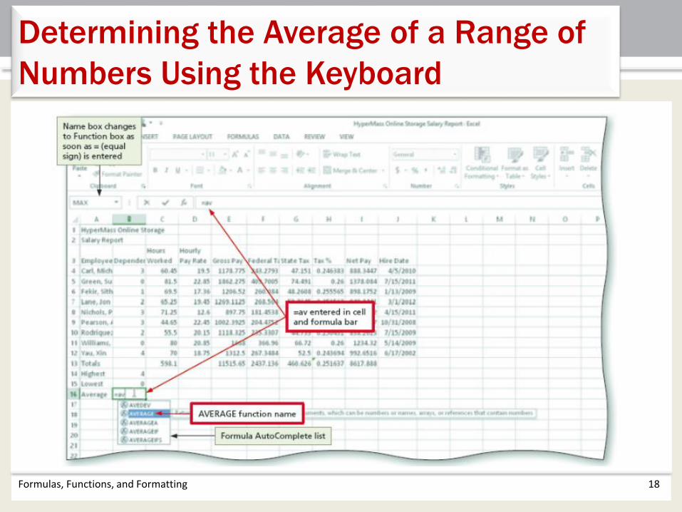
Determining the Average of a Range of
Numbers Using the Keyboard
• Select the cell that will contain the average • Type =av in the cell to display the Formula
AutoComplete list Press the DOWN ARROW key to highlight the required formula
• Double-tap or double-click AVERAGE in the Formula AutoComplete list to select the function
• Select the range to be averaged to insert the range as the argument to the function
• Tap or click the Enter box to compute the average of the numbers in the selected range and display the result in the selected cell
Formulas, Functions, and Formatting 18
Determining the Average of a Range of
Numbers Using the Keyboard

Formulas, Functions, and Formatting 19
Verifying a Formula using Range Finder
• Double-tap or double-click a cell to activate Range Finder
• Press the ESC key to quit Range Finder and then tap or click anywhere in the worksheet to deselect the current cell
Formulas, Functions, and Formatting 20
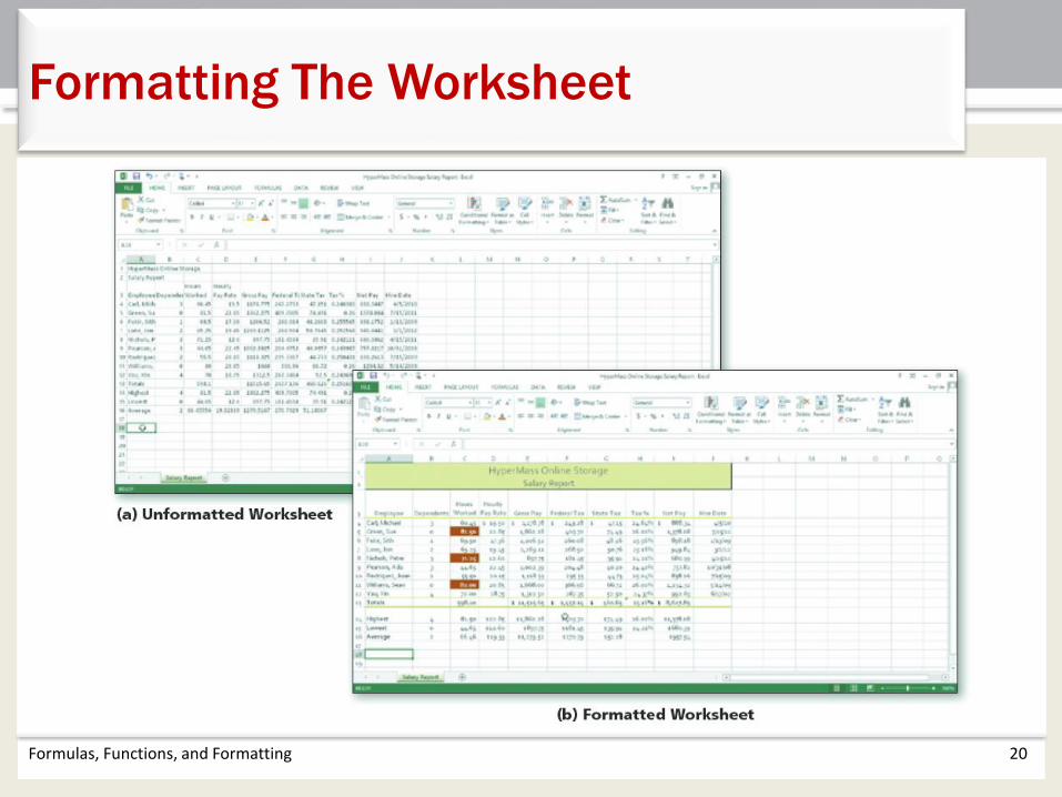
Formatting The Worksheet
Formulas, Functions, and Formatting 21
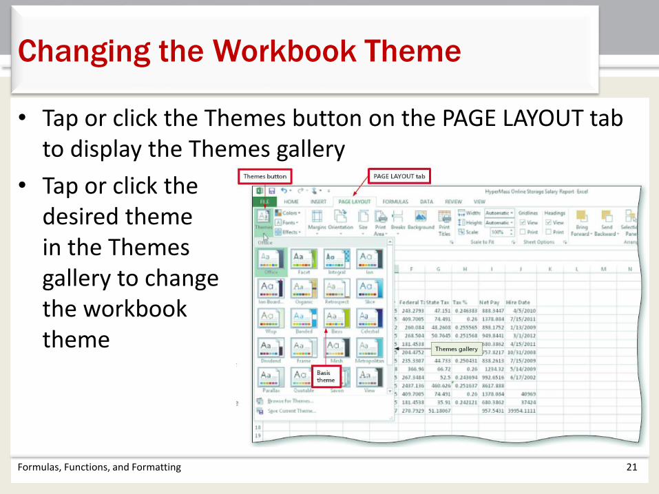
Changing the Workbook Theme
• Tap or click the Themes button on the PAGE LAYOUT tab to display the Themes gallery
• Tap or click the desired theme in the Themes gallery to change the workbook theme

• Select the range to color and then tap or click the Fill Color arrow on the HOME tab to display the Fill Color gallery
• Tap or click a color to select it and change the background color of the range of cells
• Tap or click the Borders arrow on the HOME tab to display the Borders gallery
• Tap or click a border in the Borders gallery to select it and display a border around the selected range
Formulas, Functions, and Formatting 22
Changing the Background Color and Applying a
Box Border to the Worksheet Title and Subtitle

Formulas, Functions, and Formatting 23
Changing the Background Color and Applying a
Box Border to the Worksheet Title and Subtitle

Formulas, Functions, and Formatting 24
Formatting Dates and Centering Data in
Cells
• Select the range to contain the new date format
• Tap or click the Format Cells: Number Format Dialog Box Launcher in the HOME tab to display the dialog box
• If necessary, tap or click the NUMBER tab and tap or click Date in the Category list, and then tap or click a date type to choose the format for the selected range
• Tap or click the NUMBER tab and then tap or click Date in the Category list to choose the format for the selected range
• Tap or click the OK button to format the dates in the current column using the selected date format style
• Select the range to be centered and then tap or click the Center button on the HOME tab to center the data in the selected range

Formulas, Functions, and Formatting 25
Formatting Dates and Centering Data in Cells
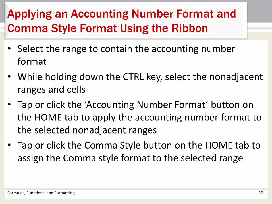
• Select the range to contain the accounting number format
• While holding down the CTRL key, select the nonadjacent ranges and cells
• Tap or click the ‘Accounting Number Format’ button on the HOME tab to apply the accounting number format to the selected nonadjacent ranges
• Tap or click the Comma Style button on the HOME tab to assign the Comma style format to the selected range
Formulas, Functions, and Formatting 26
Applying an Accounting Number Format and
Comma Style Format Using the Ribbon

Formulas, Functions, and Formatting 27
Applying an Accounting Number Format and
Comma Style Format Using the Ribbon

Formulas, Functions, and Formatting 28
Applying a Currency Style Format with a Floating
Dollar Sign Using the Format Cells Dialog Box
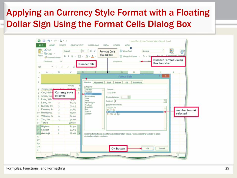
• Select the range to format and then tap or click the Number Format Dialog Box Launcher in the HOME tab to display the Format Cells dialog box
• If necessary, tap or click the NUMBER tab to display the Number sheet
• Tap or click Currency in the Category list to select the necessary number format category and then tap or click a style in the Negative numbers list to select the desired currency format
• Tap or click the OK button to assign the currency style format to the selected ranges
Formulas, Functions, and Formatting 29
Applying an Currency Style Format with a Floating
Dollar Sign Using the Format Cells Dialog Box

• Select the range to format
• Tap or click the Percent Style button in the HOME tab to display the numbers in the selected range as a rounded whole percent
• Tap or click the Increase Decimal button in the HOME tab two times to display the numbers in the selected range with two decimal places
Formulas, Functions, and Formatting 30
Applying Percent Style Format and Using
the Increase Decimal Button

• Select the range to which you wish to apply conditional formatting
• Tap or click the Conditional Formatting button on the HOME tab to display the Conditional Formatting list
• Tap or click New Rule in the Conditional Formatting list to display the New Formatting Rule dialog box
• Tap or click the desired rule type in the Select a Rule Type area
• Select and type the desired values in the Edit the Rule Description area
Formulas, Functions, and Formatting 31
Applying Conditional Formatting

Formulas, Functions, and Formatting 32
Applying Conditional Formatting

Formulas, Functions, and Formatting 33
Conditional Formatting Operators
• Drag through column headings to select the columns
• Tap or point to the boundary on the rightmost column heading to cause the pointer to become a split double arrow
• Double-tap or double-click the right boundary of the column to change the width of the selected columns to best fit
• To resize a column by dragging, point to the boundary of the right side of the column heading. When the mouse pointer changes to a split double arrow, drag to the desired width, and then Lift your finger or release the mouse button to change the column widths
Formulas, Functions, and Formatting 34
Changing the Column Width

Formulas, Functions, and Formatting 35
Changing the Column Width

• Tap or point to the boundary below the row heading to resize
• Drag the boundary to the desired row height and then release the mouse button
• Lift your finger or release the mouse button to change the row height
Formulas, Functions, and Formatting 36
Changing the Row Height

• Tap or click cell A1 so that the spell checker begins at the beginning of the worksheet
• Tap or click the Spelling button on the REVIEW tab to run the spell checker and display the misspelled words in the Spelling dialog box
• Apply the desired action to each misspelled word
• When the spell checker is finished, Tap or click the Close button
Formulas, Functions, and Formatting 37
Checking Spelling on the Worksheet

Formulas, Functions, and Formatting 38
Checking Spelling on the Worksheet

• Tap or click the Page Layout button on the status bar to view the worksheet in Page Layout view
• Tap or click the Adjust Margins button on the PAGE LAYOUT tab to display the Margins gallery
• Tap or click the desired margin style to change the worksheet margins to the selected style
• Tap or click above cell A1 in the center area of the Header area
• Type the desired worksheet header, and then press the ENTER key
Formulas, Functions, and Formatting 39
Changing the Worksheet’s Margins, Header,
and Orientation in Page Layout View

Formulas, Functions, and Formatting 40
Changing the Worksheet’s margins, header,
and Orientation in Page Layout View

• Tap or click the ‘Change Page Orientation’ button on the PAGE LAYOUT tab to display the Change Page Orientation gallery
• Tap or click the desired orientation in the Orientation gallery to change the worksheet’s orientation
Formulas, Functions, and Formatting 41
Changing the Worksheet’s margins, header,
and Orientation in Page Layout View
Formulas, Functions, and Formatting 42
Printing a Section of the Worksheet
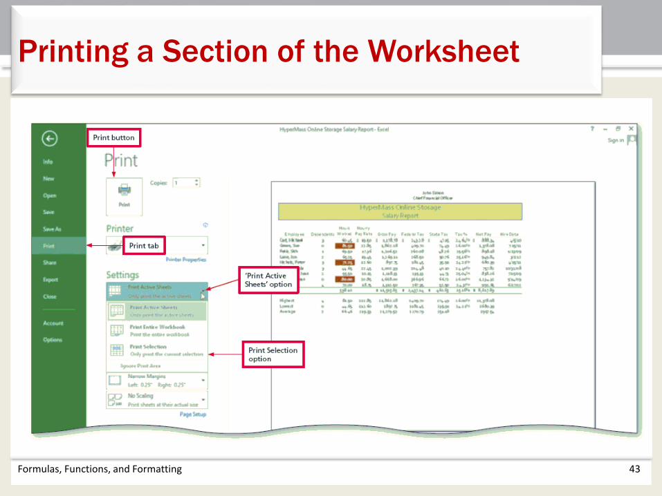
• Select the range to print
• Tap or click FILE on the ribbon to open Backstage view
• Tap or click the Print tab to display the Print gallery
• Tap or click ‘Print Active Sheets’ in the Settings area on the PRINT tab to display a list of printing options
• Tap or click Print Selection to print the selected range
• Tap or click the Print button in the Print gallery to print the selected range of the worksheet
• Tap or click the Normal button on the status bar to return to Normal view
Formulas, Functions, and Formatting 43
Printing a Section of the Worksheet
Formulas, Functions, and Formatting 44
Displaying the Formulas in the Worksheet
and Fitting the Printout on One Page
• Press CTRL+ACCENT MARK (`) to display the worksheet with formulas
• Tap or click the Page Setup Dialog Box Launcher on the PAGE LAYOUT tab to display the Page Setup dialog box
• If necessary, tap or click the desired Orientation in the Page sheet to select it
• If necessary, tap or click Fit to in the Scaling area to select it• Tap or click the Print button to print the formulas in the worksheet
on one page. If necessary, in the Backstage view, select the Print Active Sheets option in the Settings area of the Print gallery
• When Excel displays the Backstage view, tap or click the Print button to print the worksheet
• After viewing and printing the formulas version, press CTRL+ACCENT MARK (`) to display the values version

Formulas, Functions, and Formatting 45
Displaying the Formulas in the Worksheet
and Fitting the Printout on One Page

Chapter Summary
Formulas, Functions, and Formatting 46
• Enter formulas using the keyboard
• Enter formulas using Point mode
• Apply the MAX, MIN, and AVERAGE functions
• Verify a formula using Range Finder
• Apply a theme to a workbook
• Apply a date format to a cell or range

Chapter Summary
Formulas, Functions, and Formatting 47
• Add conditional formatting to cells
• Change column width and row height
• Check the spelling on a worksheet
• Change margins and headers in Page Layout view
• Preview and print versions and sections of a worksheet
Chapter 2 Complete
Microsoft
Excel 2013


