HAL Id: hal-01343687https://hal.archives-ouvertes.fr/hal-01343687v2

Submitted on 21 Jun 2019

HAL is a multi-disciplinary open accessarchive for the deposit and dissemination of sci-entific research documents, whether they are pub-lished or not. The documents may come fromteaching and research institutions in France orabroad, or from public or private research centers.

L’archive ouverte pluridisciplinaire HAL, estdestinée au dépôt et à la diffusion de documentsscientifiques de niveau recherche, publiés ou non,émanant des établissements d’enseignement et derecherche français ou étrangers, des laboratoirespublics ou privés.

Microwave Tomographic Imaging of CerebrovascularAccidents by Using High-Performance Computing

Pierre-Henri Tournier, Ioannis Aliferis, Marcella Bonazzoli, Maya de Buhan,Marion Darbas, Victorita Dolean, Frédéric Hecht, Pierre Jolivet, Ibtissam El

Kanfoud, Claire Migliaccio, et al.

To cite this version:Pierre-Henri Tournier, Ioannis Aliferis, Marcella Bonazzoli, Maya de Buhan, Marion Darbas, et al..Microwave Tomographic Imaging of Cerebrovascular Accidents by Using High-Performance Comput-ing. Parallel Computing, Elsevier, 2019, 85, pp.88-97. 10.1016/j.parco.2019.02.004. hal-01343687v2

Microwave Tomographic Imaging of Cerebrovascular Accidents by UsingHigh-Performance Computing

P.-H. Tourniera, I. Aliferisb, M. Bonazzolij, M. de Buhand, M. Darbase, V. Doleanc,f, F. Hechta, P. Jolivetg,I. El Kanfoudb, C. Migliacciob, F. Natafa, Ch. Pichotb,i, S. Semenovh

aSorbonne Universite, Universite Paris-Diderot SPC, CNRS, Inria, Laboratoire Jacques-Louis Lions, equipe Alpines, F-75005 ParisbUniversite Cote d’Azur, CNRS, LEAT, FrancecUniversite Cote d’Azur, CNRS, LJAD, France

dMAP5, UMR CNRS 8145, Universite Paris-Descartes, Sorbonne Paris Cite, FranceeLAMFA, UMR CNRS 7352, Universite de Picardie Jules Verne, Amiens, France

fDept of Maths and Stats, University of Strathclyde, Glasgow, UKgIRIT, UMR CNRS 5505, Toulouse, France

hEMTensor GmbH, TechGate, 1220 Vienna, AustriaiSchool of Innovation, Design and Engineering, Malardalen University, Sweden

jINRIA Saclay Ile-de-France, CMAP, Ecole Polytechnique, Palaiseau, France

Abstract

The motivation of this work is the detection of cerebrovascular accidents by microwave tomographic imaging. Thisrequires the solution of an inverse problem relying on a minimization algorithm (for example, gradient-based), wheresuccessive iterations consist in repeated solutions of a direct problem. The reconstruction algorithm is extremelycomputationally intensive and makes use of efficient parallel algorithms and high-performance computing. The fea-sibility of this type of imaging is conditioned on one hand by an accurate reconstruction of the material properties ofthe propagation medium and on the other hand by a considerable reduction in simulation time. Fulfilling these tworequirements will enable a very rapid and accurate diagnosis. From the mathematical and numerical point of view, thismeans solving Maxwell’s equations in time-harmonic regime by appropriate domain decomposition methods, whichare naturally adapted to parallel architectures.

Keywords: inverse problem, scalable preconditioners, Maxwell’s equations, microwave imaging

1. Introduction

A stroke, also known as cerebrovascular accident, is a disturbance in the blood supply to the brain caused by ablocked or burst blood vessel. As a consequence, cerebral tissues are deprived of oxygen and nutrients. This resultsin a rapid loss of brain functions and often death. Strokes are classified into two major categories: ischemic (85% ofstrokes) and hemorrhagic (15% of strokes). During an acute ischemic stroke, the blood supply to a part of the brainis interrupted by thrombosis - the formation of a blood clot in a blood vessel - or by an embolism elsewhere in thebody. A hemorrhagic stroke occurs when a blood vessel bursts inside the brain, increasing pressure in the brain andinjuring brain cells. The two types of strokes result in opposite variations of the dielectric properties of the affectedtissues. How quickly one can detect and characterize the stroke is of fundamental importance for the survival ofthe patient. The quicker the treatment is, the more reversible the damage and the better the chances of recovery are.Moreover, the treatment of ischemic stroke consists in thinning the blood (anticoagulants) and can be fatal if the strokeis hemorrhagic. Therefore, it is vital to make a clear distinction between the two types of strokes before treating thepatient. Moreover, ideally one would want to monitor continuously the effect of the treatment on the evolution of thestroke during the hospitalization. The two most used imaging techniques for strokes diagnosis are MRI (magneticresonance imaging) and CT scan (computerized tomography scan). One of their downsides is that the travel timefrom the patient’s home to the hospital is lost. Moreover, the cost and the lack of portability of MRI and the harmfulcharacter of CT scan, which uses ionizing radiation and thus cannot be used repeatedly, make them unsuitable for acontinuous monitoring at the hospital during treatment.

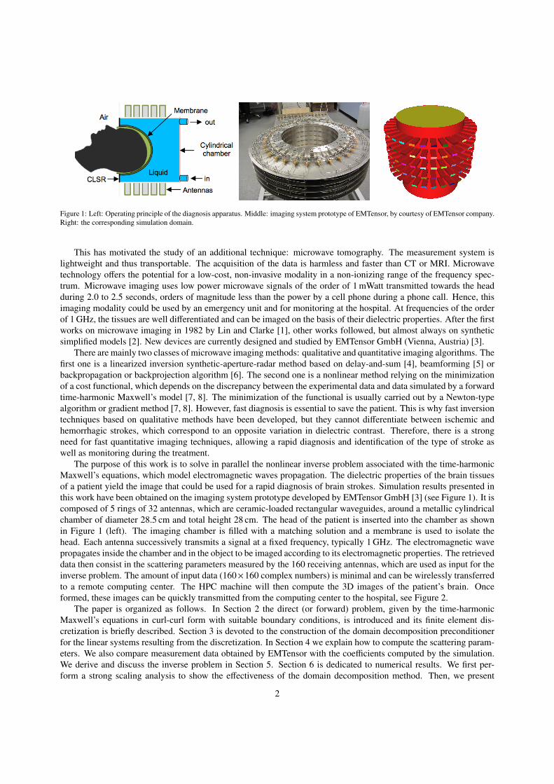
Figure 1: Left: Operating principle of the diagnosis apparatus. Middle: imaging system prototype of EMTensor, by courtesy of EMTensor company.Right: the corresponding simulation domain.

This has motivated the study of an additional technique: microwave tomography. The measurement system islightweight and thus transportable. The acquisition of the data is harmless and faster than CT or MRI. Microwavetechnology offers the potential for a low-cost, non-invasive modality in a non-ionizing range of the frequency spec-trum. Microwave imaging uses low power microwave signals of the order of 1 mWatt transmitted towards the headduring 2.0 to 2.5 seconds, orders of magnitude less than the power by a cell phone during a phone call. Hence, thisimaging modality could be used by an emergency unit and for monitoring at the hospital. At frequencies of the orderof 1 GHz, the tissues are well differentiated and can be imaged on the basis of their dielectric properties. After the firstworks on microwave imaging in 1982 by Lin and Clarke [1], other works followed, but almost always on syntheticsimplified models [2]. New devices are currently designed and studied by EMTensor GmbH (Vienna, Austria) [3].

There are mainly two classes of microwave imaging methods: qualitative and quantitative imaging algorithms. Thefirst one is a linearized inversion synthetic-aperture-radar method based on delay-and-sum [4], beamforming [5] orbackpropagation or backprojection algorithm [6]. The second one is a nonlinear method relying on the minimizationof a cost functional, which depends on the discrepancy between the experimental data and data simulated by a forwardtime-harmonic Maxwell’s model [7, 8]. The minimization of the functional is usually carried out by a Newton-typealgorithm or gradient method [7, 8]. However, fast diagnosis is essential to save the patient. This is why fast inversiontechniques based on qualitative methods have been developed, but they cannot differentiate between ischemic andhemorrhagic strokes, which correspond to an opposite variation in dielectric contrast. Therefore, there is a strongneed for fast quantitative imaging techniques, allowing a rapid diagnosis and identification of the type of stroke aswell as monitoring during the treatment.

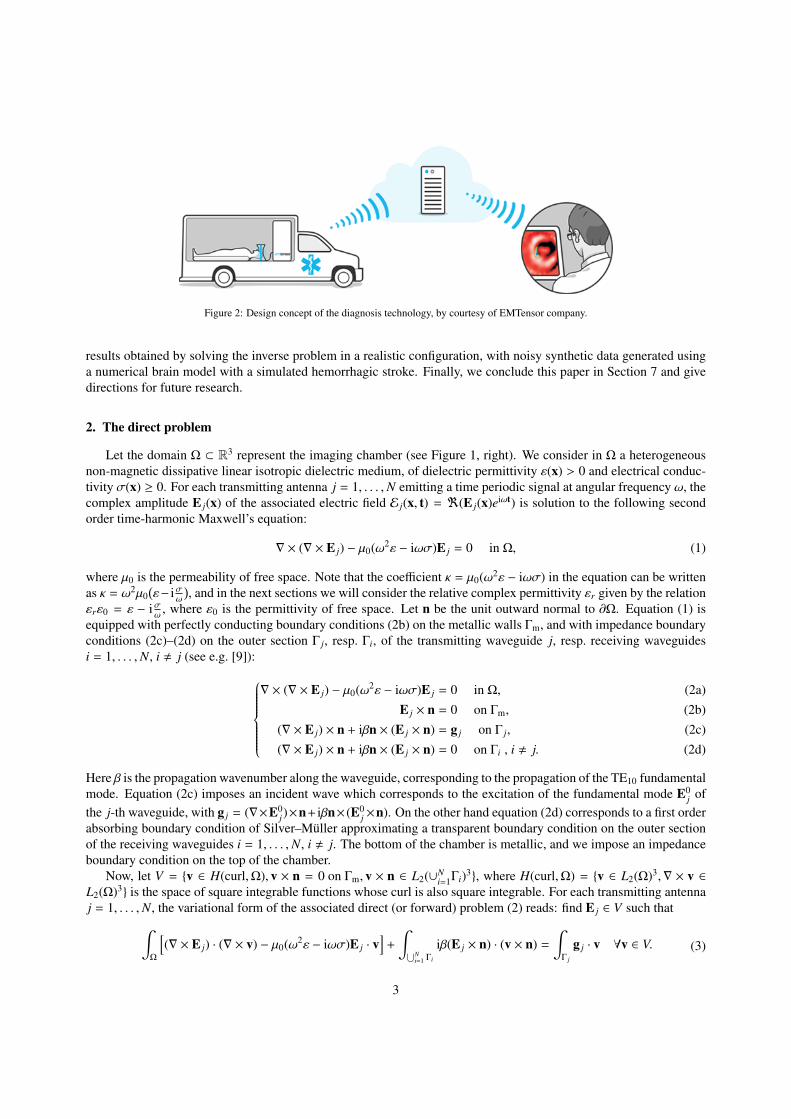
The purpose of this work is to solve in parallel the nonlinear inverse problem associated with the time-harmonicMaxwell’s equations, which model electromagnetic waves propagation. The dielectric properties of the brain tissuesof a patient yield the image that could be used for a rapid diagnosis of brain strokes. Simulation results presented inthis work have been obtained on the imaging system prototype developed by EMTensor GmbH [3] (see Figure 1). It iscomposed of 5 rings of 32 antennas, which are ceramic-loaded rectangular waveguides, around a metallic cylindricalchamber of diameter 28.5 cm and total height 28 cm. The head of the patient is inserted into the chamber as shownin Figure 1 (left). The imaging chamber is filled with a matching solution and a membrane is used to isolate thehead. Each antenna successively transmits a signal at a fixed frequency, typically 1 GHz. The electromagnetic wavepropagates inside the chamber and in the object to be imaged according to its electromagnetic properties. The retrieveddata then consist in the scattering parameters measured by the 160 receiving antennas, which are used as input for theinverse problem. The amount of input data (160×160 complex numbers) is minimal and can be wirelessly transferredto a remote computing center. The HPC machine will then compute the 3D images of the patient’s brain. Onceformed, these images can be quickly transmitted from the computing center to the hospital, see Figure 2.

The paper is organized as follows. In Section 2 the direct (or forward) problem, given by the time-harmonicMaxwell’s equations in curl-curl form with suitable boundary conditions, is introduced and its finite element dis-cretization is briefly described. Section 3 is devoted to the construction of the domain decomposition preconditionerfor the linear systems resulting from the discretization. In Section 4 we explain how to compute the scattering param-eters. We also compare measurement data obtained by EMTensor with the coefficients computed by the simulation.We derive and discuss the inverse problem in Section 5. Section 6 is dedicated to numerical results. We first per-form a strong scaling analysis to show the effectiveness of the domain decomposition method. Then, we present

2

Figure 2: Design concept of the diagnosis technology, by courtesy of EMTensor company.

results obtained by solving the inverse problem in a realistic configuration, with noisy synthetic data generated usinga numerical brain model with a simulated hemorrhagic stroke. Finally, we conclude this paper in Section 7 and givedirections for future research.

2. The direct problem

Let the domain Ω ⊂ R3 represent the imaging chamber (see Figure 1, right). We consider in Ω a heterogeneousnon-magnetic dissipative linear isotropic dielectric medium, of dielectric permittivity ε(x) > 0 and electrical conduc-tivity σ(x) ≥ 0. For each transmitting antenna j = 1, . . . ,N emitting a time periodic signal at angular frequency ω, thecomplex amplitude E j(x) of the associated electric field E j(x, t) = <(E j(x)eiωt) is solution to the following secondorder time-harmonic Maxwell’s equation:

∇ × (∇ × E j) − µ0(ω2ε − iωσ)E j = 0 in Ω, (1)

where µ0 is the permeability of free space. Note that the coefficient κ = µ0(ω2ε − iωσ) in the equation can be writtenas κ = ω2µ0

(ε− iσ

ω

), and in the next sections we will consider the relative complex permittivity εr given by the relation

εrε0 = ε − iσω

, where ε0 is the permittivity of free space. Let n be the unit outward normal to ∂Ω. Equation (1) isequipped with perfectly conducting boundary conditions (2b) on the metallic walls Γm, and with impedance boundaryconditions (2c)–(2d) on the outer section Γ j, resp. Γi, of the transmitting waveguide j, resp. receiving waveguidesi = 1, . . . ,N, i , j (see e.g. [9]):

∇ × (∇ × E j) − µ0(ω2ε − iωσ)E j = 0 in Ω,

E j × n = 0 on Γm,

(∇ × E j) × n + iβn × (E j × n) = g j on Γ j,

(∇ × E j) × n + iβn × (E j × n) = 0 on Γi , i , j.

(2a)(2b)(2c)(2d)

Here β is the propagation wavenumber along the waveguide, corresponding to the propagation of the TE10 fundamentalmode. Equation (2c) imposes an incident wave which corresponds to the excitation of the fundamental mode E0

j ofthe j-th waveguide, with g j = (∇×E0

j )×n+ iβn× (E0j ×n). On the other hand equation (2d) corresponds to a first order

absorbing boundary condition of Silver–Muller approximating a transparent boundary condition on the outer sectionof the receiving waveguides i = 1, . . . ,N, i , j. The bottom of the chamber is metallic, and we impose an impedanceboundary condition on the top of the chamber.

Now, let V = v ∈ H(curl,Ω), v × n = 0 on Γm, v × n ∈ L2(∪Ni=1Γi)3, where H(curl,Ω) = v ∈ L2(Ω)3,∇ × v ∈

L2(Ω)3 is the space of square integrable functions whose curl is also square integrable. For each transmitting antennaj = 1, . . . ,N, the variational form of the associated direct (or forward) problem (2) reads: find E j ∈ V such that∫

Ω

[(∇ × E j) · (∇ × v) − µ0(ω2ε − iωσ)E j · v

]+

∫⋃N

i=1 Γi

iβ(E j × n) · (v × n) =

∫Γ j

g j · v ∀v ∈ V. (3)

3

2.1. Edge finite element discretization

In order to discretize problem (3) by a finite element method, consider a tetrahedral mesh T of the computationaldomain Ω. Nedelec edge elements [10] are finite elements particularly suited for the approximation of the electricfield. Indeed, they ensure continuity of the tangential component of the field and the finite dimensional subspace Vh

generated by Nedelec basis functions is included in H(curl,Ω). Nedelec elements are called edge elements because,at the lowest order (degree r = 1), basis functions and degrees of freedom are associated with the (oriented) edges ofthe mesh T : the degrees of freedom are circulations of the field along the edges.

The finite element discretization of the variational problem (3) produces linear systems

Au j = b j, (4)

one for each transmitting antenna j = 1, . . . ,N. Note that the matrix A is the same for all transmitting antennas, butthe right-hand side b j is different.

3. Domain decomposition preconditioning

Since the matrix A of the linear systems (4) can be ill-conditioned, we need a robust and efficient preconditionerfor the iterative solver (GMRES). Here we employ domain decomposition preconditioners, which are extensivelydescribed in [11], as they are naturally suited to parallel computing. The construction of the chosen domain decom-position preconditioner is presented in the following.

First, the mesh T is partitioned into NS non-overlapping meshes Ti16i6NS using standard graph partitionerssuch as SCOTCH [12] or METIS [13]. If δ is a positive integer, the overlapping decomposition T δ

i 16i6NS is definedrecursively as follows: T δ

i is obtained by including all tetrahedra of T δ−1i plus all adjacent tetrahedra of T δ−1

i ; forδ = 0, T δ

i = Ti. Note that the number of layers in the overlap is then 2δ. Now, let Vδi 16i6NS be the local edge finite

element spaces defined on T δi 16i6NS , δ > 0. Consider the restrictions Ri16i6NS from Vh to Vδ

i 16i6NS , and a localpartition of unity Di16i6NS such that

NS∑i=1

RTi DiRi = In×n. (5)

Algebraically speaking, if n is the global number of unknowns and ni16i6NS are the numbers of unknowns for eachlocal finite element space, then Ri is a Boolean matrix of size ni × n, and Di is a diagonal matrix of size ni × ni, for all1 6 i 6 NS . Note that RT

i , the transpose of Ri, is a n × ni matrix that gives the extension by 0 from Vδi to Vh.

Using these matrices, one can define the following one-level preconditioner, called Optimized Restricted AdditiveSchwarz preconditioner (ORAS) [14, 15]:

M−1ORAS =

NS∑i=1

RTi DiB−1

i Ri, (6)

where Bi16i6NS are local operators corresponding to the subproblems with impedance boundary conditions (∇ ×E) × n + ikn × (E × n) on the interfaces between subdomains, where k = ω

√µ0ε is the wavenumber. It is important

to note that when a direct solver is used to compute the action of B−1i on multiple vectors, this can be done in a single

forward elimination and backward substitution. More details on the solution of linear systems with multiple right-hand sides are given in Section 6. The preconditioner M−1

ORAS (6) is naturally parallel since its assembly requires theconcurrent factorization of each Bi16i6NS , which are typically stored locally on different processes in a distributedcomputing context. Likewise, applying (6) to a distributed vector only requires peer-to-peer communications betweenneighboring subdomains, and a local forward elimination and backward substitution. See chapter 8 of [11] for a moredetailed analysis.

3.1. Software stack

All operators related to the domain decomposition method can be generated using finite element Domain-SpecificLanguages (DSL). Here we use FreeFem++ [16] (http://www.freefem.org/ff++/) since it has already been

4

proven that it can enable large-scale simulations using overlapping Schwarz methods [17] when used in combi-nation with the library HPDDM [18] (High-Performance unified framework for Domain Decomposition Methods,https://github.com/hpddm/hpddm). HPDDM implements several domain decomposition methods such as RAS,ORAS, FETI, and BNN. It uses multiple levels of parallelism: communication between subdomains is based on theMessage Passing Interface (MPI), and computations in the subdomains can be executed on several threads by callingoptimized BLAS libraries (such as Intel MKL), or shared-memory direct solvers like PARDISO. Domain decom-position methods naturally offer good parallel properties on distributed architectures. The computational domain isdecomposed into subdomains in which concurrent computations are performed. The coupling between subdomainsrequires communications between computing nodes via messages. The strong scalability of the ORAS preconditioneras implemented in HPDDM for the direct problem presented in Section 2 will be assessed in Section 6.

3.2. Partition of unityHere we describe the construction of the partition of unity (5) in more details, as its construction in the context of

Nedelec edge elements is non-trivial.The starting point is the construction of partition of unity functions χi16i6NS for the classical P1 linear nodal finite

element, whose degrees of freedom are the values at the nodes of the mesh. First of all, we define for i = 1, . . . ,NS

the function χi as the continuous piecewise linear function on T , with support contained in T δi , such that

χi =

1 at all nodes of T 0i ,

0 at all nodes of T δi \ T

0i .

The function χi can then be defined as the continuous piecewise linear function on T , with support contained in T δi ,

such that its (discrete) value for each degree of freedom is evaluated by:

χi =χi

NS∑j=1

χ j

. (7)

Thus, we have∑NS

i=1 χi = 1 both at the discrete and continuous level. Remark that if δ > 1, not only the function χi

but also its derivative is equal to zero on the border of T δi . This is essential for a good convergence if Robin-type

boundary conditions (such as impedance boundary conditions) are chosen as transmission conditions at the interfacesbetween subdomains. Indeed, if this property is satisfied, the continuous version of the ORAS algorithm is equivalentto P. L. Lions’ algorithm (see [14] and [11] §2.3.2). Note that in the practical implementation, the functions χi and χi

are constructed locally on T δi , the relevant contribution of the χ j in (7) being on T δ

j ∩Tδi . This removes all dependency

on the global mesh T , which could be otherwise problematic at large scales.Now, the degrees of freedom of Nedelec finite elements are associated with the edges of the mesh. For these finite

elements, we can build a geometric partition of unity based on the support of the degrees of freedom (the edges of themesh): the entries of the diagonal matrices Di, i = 1, . . . ,NS are obtained for each degree of freedom by interpolatingthe piecewise linear function χi at the midpoint of the corresponding edge. The partition of unity property (5) is thensatisfied since

∑NSi=1 χi = 1.

This interpolation is obtained thanks to a new FreeFem++ scalar finite element space, which has only the in-terpolation operator (defined by one quadrature point on each edge) and no basis functions. This auxiliary finiteelement space is available by loading the plugin Element Mixte3d and is called Edge03ds0, when using the low-est order edge finite elements (Edge03d) to discretize the problem. The example script maxwell-3d.edp, availablein the directory examples++-hpddm of the FreeFem++ distribution, shows how to use these new tools for domaindecomposition with edge finite elements.

4. Computing the scattering parameters

In order to compute the numerical counterparts of the reflection and transmission coefficients obtained by themeasurement apparatus of the imaging chamber shown in Figure 1, we use the following formula, which is appropriate

5

in the case of open-ended waveguides:

S i j =

∫Γi

E j · E0i∫

Γi

|E0i |

2, i, j = 1, . . . ,N, (8)

where E0i is the TE10 fundamental mode of the i-th receiving waveguide and E j is the solution of the problem where the

j-th waveguide transmits the signal (E j denotes the complex conjugate of E j). The S i j with i , j are the transmissioncoefficients, and the S j j are the reflection coefficients. They are gathered in the scattering matrix, also called S-matrix.

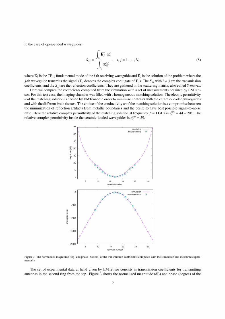
Here we compare the coefficients computed from the simulation with a set of measurements obtained by EMTen-sor. For this test case, the imaging chamber was filled with a homogeneous matching solution. The electric permittivityε of the matching solution is chosen by EMTensor in order to minimize contrasts with the ceramic-loaded waveguidesand with the different brain tissues. The choice of the conductivityσ of the matching solution is a compromise betweenthe minimization of reflection artifacts from metallic boundaries and the desire to have best possible signal-to-noiseratio. Here the relative complex permittivity of the matching solution at frequency f = 1 GHz is εgel

r = 44 − 20i. Therelative complex permittivity inside the ceramic-loaded waveguides is εcer

r = 59.

0

10

20

30

40

50

60

70

5 10 15 20 25 30

ma

gn

itu

de

(d

B)

receiver number

simulation

measurements

-2000

-1500

-1000

-500

0

5 10 15 20 25 30

phase (

degre

e)

receiver number

simulation

measurements

Figure 3: The normalized magnitude (top) and phase (bottom) of the transmission coefficients computed with the simulation and measured experi-mentally.

The set of experimental data at hand given by EMTensor consists in transmission coefficients for transmittingantennas in the second ring from the top. Figure 3 shows the normalized magnitude (dB) and phase (degree) of the

6

complex coefficients S i j corresponding to a transmitting antenna in the second ring from the top and to the 31 receiv-ing antennas in the middle ring (note that measured coefficients are available only for 17 receiving antennas). Themagnitude in dB is calculated as 20 log10(|S i j|). The normalization is done by dividing every transmission coefficientby the transmission coefficient corresponding to the receiving antenna directly opposite to the transmitting antenna,which is thus set to 1. Since we normalize with respect to the coefficient having the lowest expected magnitude, themagnitude of the transmission coefficients displayed in Figure 3 is larger than 0 dB. We can see that the transmissioncoefficients computed from the simulation are in very good agreement with the measurements.

5. The inverse problem

The inverse problem that we consider consists in finding the unknown dielectric permittivity ε(x) and conductivityσ(x) in Ω, such that the solutions E j, j = 1, . . . ,N of problem (2) lead to corresponding scattering parameters S i j (8)that coincide with the measured scattering parameters S mes

i j , for i, j = 1, . . . ,N. In the following, we present theinverse problem in the continuous setting for clarity.

Let κ = µ0(ω2ε − iωσ) be the unknown complex parameter of our inverse problem, and let us denote by E j(κ)the solution of the direct problem (2) with dielectric permittivity ε and conductivity σ. The corresponding scatteringparameters will be denoted by S i j(κ) for i, j = 1, . . . ,N:

S i j(κ) =

∫Γi

E j(κ) · E0i∫

Γi

|E0i |

2, i, j = 1, . . . ,N.

The misfit of the parameter κ to the data can be defined through the following functional:

J(κ) =12

N∑j=1

N∑i=1

∣∣∣S i j(κ) − S mesi j

∣∣∣2 =12

N∑j=1

N∑i=1

∣∣∣∣∣∣∣∣∣∣∣∫

Γi

E j(κ) · E0i∫

Γi

|E0i |

2− S mes

i j

∣∣∣∣∣∣∣∣∣∣∣2

. (9)

In a classical way, solving the inverse problem then consists in minimizing the functional J with respect to the param-eter κ. Computing the differential of J in a given arbitrary direction δκ yields

DJ(κ, δκ) =

N∑j=1

N∑i=1

<

(S i j(κ) − S mes

i j

)∫

Γi

δE j(κ) · E0i∫

Γi

|E0i |

2

, δκ ∈ C,

where δE j(κ) is the solution of the following linearized problem:∇ × (∇ × δE j) − κδE j = δκE j in Ω,

δE j × n = 0 on Γm,

(∇ × δE j) × n + iβn × (δE j × n) = 0 on Γi , i = 1, . . . ,N.(10)

We now use the adjoint approach in order to simplify the expression of DJ. This will allow us to compute thegradient efficiently after discretization, with a number of computations independent of the size of the parameter space.

7

Considering the variational formulation of problem (10) with a test function F and integrating by parts, we get∫Ω

δκE j · F =

∫Ω

(∇ × (∇ × δE j) − κδE j

)· F

=

∫Ω

(∇ × (∇ × F) − κF) · δE j −

∫∂Ω

((∇ × δE j) × n) · F +

∫∂Ω

((∇ × F) × n) · δE j

=

∫Ω

(∇ × (∇ × F) − κF) · δE j +

N∑i=1

∫Γi

iβ(n × (F × n)) · δE j

+

∫Γm

(∇ × δE j) · (F × n) +

N∑i=1

∫Γi

((∇ × F) × n) · δE j.

Introducing the solution F j(κ) of the following adjoint problem

∇ × (∇ × F j) − κF j = 0 in Ω,

F j × n = 0 on Γm,

(∇ × F j) × n + iβn × (F j × n) =(S i j(κ) − S mes

i j )∫Γi

|E0i |

2E0

i on Γi , i = 1, . . . ,N,(11)

we get ∫Ω

δκE j · F j =

N∑i=1

(S i j(κ) − S mesi j )

∫Γi

E0i · δE j∫

Γi

|E0i |

2.

Finally, the differential of J can be computed as

DJ(κ, δκ) = <

∫Ω

δκ

N∑j=1

E j · F j

.We can then compute the gradient to use in a gradient-based local optimization algorithm. The numerical results

presented in Section 6 are obtained using a limited-memory Broyden-Fletcher-Goldfarb-Shanno (L-BFGS) algorithm.Note that every evaluation of J requires the solution of the state problem (2) while the computation of the gradientrequires the solution of (2) as well as the solution of the adjoint problem (11). Moreover, the state and adjointproblems use the same operator. Therefore, the computation of the gradient only needs the assembly of one matrixand its associated domain decomposition preconditioner.

Numerical results for the reconstruction of a hemorrhagic stroke from synthetic data are presented in the nextsection. The functional J considered in the numerical results is slightly different from (9), as we add a normalizationterm for each pair (i, j) as well as a Tikhonov regularizing term:

J(κ) =12

N∑j=1

N∑i=1

∣∣∣S i j(κ) − S mesi j

∣∣∣2∣∣∣S emptyi j

∣∣∣2 +α

2

∫Ω

|∇κ|2, (12)

where S emptyi j refers to the coefficients computed from the simulation with the empty chamber, that is the chamber

filled only with the homogeneous matching solution as described in the previous section, with no object inside. In thisway, the contribution of each pair (i, j) in the misfit functional is normalized and does not depend on the amplitudeof the coefficient, which can vary greatly between pairs (i, j) as displayed in Figure 3. The Tikhonov regularizingterm aims at reducing the effects of noise in the data. For now, the regularization parameter α is chosen empiricallyso as to obtain a visually good compromise between reducing the effects of noise and keeping the reconstructedimage pertinent. All calculations carried out in this section can be accommodated in a straightforward manner todefinition (12) of the functional.

8

256 512 1 024 2 048

500

200

50

10

(43)

(53)

(64)(81)

# of subdomains

Tim

eto

solu

tion

(inse

cond

s)

Setup Solve Linear speedup

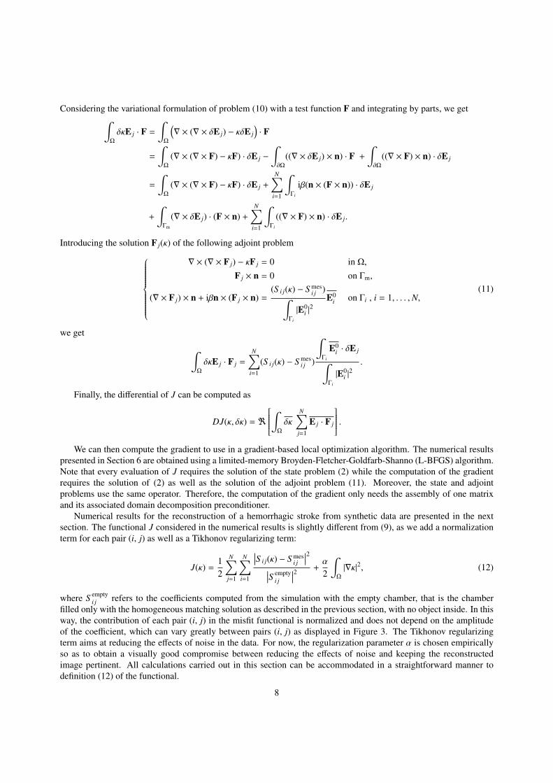
Figure 4: Strong scaling experiment. Colors indicate the fraction of the total time spent in the setup and solution phases. The number of GMRESiterations is reported in parentheses.

NS Setup Solve # of iterations Speedup256 293.36 73.06 43 1512 95.11 36.92 53 2.8

1,024 35.13 20.55 64 6.62,048 25.89 12.77 81 9.5

Table 1: Strong scaling experiment. Timings (in seconds) of the setup and solution phases.

6. Numerical results

Results in this paper were obtained on Curie, a system composed of 5,040 nodes made of two eight-core IntelSandy Bridge processors clocked at 2.7 GHz. The interconnect is an InfiniBand QDR full fat tree and the MPI imple-mentation used was BullxMPI version 1.2.8.4. Intel compilers and Math Kernel Library in their version 16.0.2.181were used for all binaries and shared libraries, and as the linear algebra backend for dense computations. One-levelpreconditioners such as (6), whose action on a vector is implemented by HPDDM, require the use of a sparse directsolver. In the following experiments, we have been using either PARDISO [19] from Intel MKL or MUMPS [20].All linear systems resulting from the edge finite elements discretization are solved by GMRES right-preconditionedwith ORAS (6) as implemented in HPDDM. The GMRES algorithm is stopped once the unpreconditioned relativeresidual is lower than 10−8. First, we perform a strong scaling analysis in order to assess the efficiency of our precondi-tioner. Then, we assess the feasibility of the microwave imaging technique presented in this paper for stroke detectionand monitoring through a numerical example in a realistic configuration. We use synthetic data corresponding to anumerical model of a virtual human head with a simulated hemorrhagic stroke as input for the inverse problem.

6.1. Scaling analysisUsing the domain decomposition preconditioner (6), we solve the direct problem corresponding to the setting

of Section 4 where the chamber is filled with a homogeneous matching solution. We consider a right-hand sidecorresponding to a transmitting antenna in the second ring from the top. Given a fine mesh of the domain composedof 82 million tetrahedra, we increase the number of MPI processes to solve the linear system of 96 million double-precision complex unknowns yielded by the discretization of Maxwell’s equation using edge elements. The globalunstructured mesh is partitioned using SCOTCH [12] and the local solver is PARDISO from Intel MKL. We use onesubdomain and two OpenMP threads per MPI process. Results are reported in Table 1 and illustrated in Figure 4 witha plot of the time to solution including both the setup and solution phases on 256 up to 2048 subdomains. The setuptime corresponds to the maximum time spent for the factorization of the local subproblem matrix Bi in (6) over allsubdomains, while the solution time corresponds to the time needed to solve the linear system with GMRES. We areable to obtain very good speedups up to 4096 cores (2048 subdomains) on Curie, with a superlinear speedup of 9.5

9

between 256 and 2048 subdomains. Indeed, for the range of process counts we are considering here, the cost of thesetup (performing exact LDLH factorizations in subdomains) is greater than the one of the solution phase. Moreover,since the cost of computing such factorizations decreases quadratically with respect to the size of the local problems,it is possible to achieve superlinear speedups in the strong-scaling regime.

6.2. Direct simulation of a hemorrhagic stroke using a virtual head model

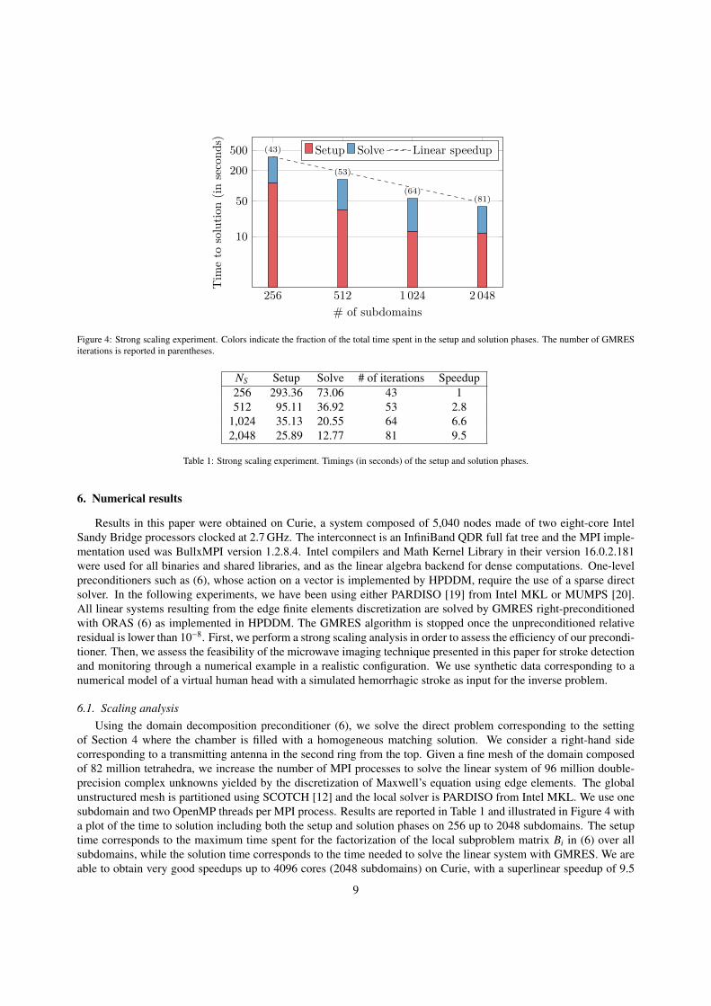
The numerical model of the virtual head comes from CT and MRI tomographic images and consists of a complexpermittivity map of 362× 434× 362 data points. Figure 5 (left) shows a sagittal section of the head. In the simulation,the head is immersed in the imaging chamber as shown in Figure 5 (right). In order to simulate a hemorrhagicstroke, a synthetic stroke is added in the form of an ellipsoid in which the value of the complex permittivity εr hasbeen increased. For this test case, the value of the permittivity in the ellipsoid is taken as the mean value betweenthe relative permittivity of the original healthy brain and the relative permittivity of blood at frequency f = 1 GHz,εblood

r = 68 − 44i. The imaging chamber is filled with a matching solution. The relative permittivity of the matchingsolution is chosen by EMTensor as explained in Section 4 and is equal to εgel

r = 44 − 20i at frequency f = 1 GHz. Inthe real setting, a special membrane fitting the shape of the head is used in order to isolate the head from the matchingmedium. We do not take this membrane into account in this synthetic test case. The synthetic data are obtained bysolving the direct problem on a mesh composed of 17.6 million tetrahedra (corresponding to approximately 20 pointsper wavelength) and consist in the transmission and reflection coefficients S i j calculated from the simulated electricfield as in (8).

Figure 5: Left: sagittal section of the brain. Right: numerical head immersed in the imaging chamber, with a simulated ellipsoid-shaped hemor-rhagic stroke.

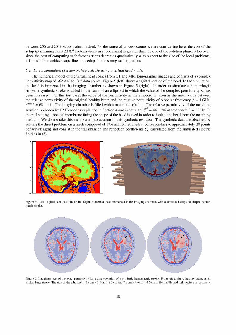
Figure 6: Imaginary part of the exact permittivity for a time evolution of a synthetic hemorrhagic stroke. From left to right: healthy brain, smallstroke, large stroke. The size of the ellipsoid is 3.9 cm × 2.3 cm × 2.3 cm and 7.7 cm × 4.6 cm × 4.6 cm in the middle and right picture respectively.

10

We simulate the evolution of the hemorrhagic stroke by increasing the size of the ellipsoid in which the value ofthe permittivity is raised. Thus, we solve the direct problem for three different complex permittivity maps, shown inFigure 6: healthy brain, small stroke and large stroke.

0 5 10 15 20 25 30 35receiver number

-120

-100

-80

-60

-40

-20

0

20

mag

nitu

de (d

B)

no stroke, TX 1small stroke, TX 1no stroke, TX 9small stroke, TX 9no stroke, TX 17small stroke, TX 17no stroke, TX 25small stroke, TX 25empty chamber

0 5 10 15 20 25 30 35receiver number

-1000

-800

-600

-400

-200

0

200

400

600

800

1000

phas

e (d

egre

e)

no stroke, TX 1small stroke, TX 1no stroke, TX 9small stroke, TX 9no stroke, TX 17small stroke, TX 17no stroke, TX 25small stroke, TX 25empty chamber

0 5 10 15 20 25 30 35receiver number

-120

-100

-80

-60

-40

-20

0

20

mag

nitu

de (d

B)

no stroke, TX 1large stroke, TX 1no stroke, TX 9large stroke, TX 9no stroke, TX 17large stroke, TX 17no stroke, TX 25large stroke, TX 25empty chamber

0 5 10 15 20 25 30 35receiver number

-1000

-800

-600

-400

-200

0

200

400

600

800

1000

phas

e (d

egre

e)

no stroke, TX 1large stroke, TX 1no stroke, TX 9large stroke, TX 9no stroke, TX 17large stroke, TX 17no stroke, TX 25large stroke, TX 25empty chamber

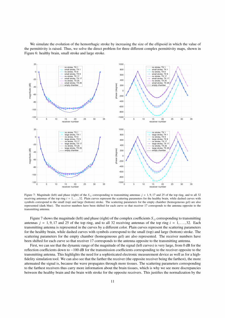
Figure 7: Magnitude (left) and phase (right) of the S i j corresponding to transmitting antennas j = 1, 9, 17 and 25 of the top ring, and to all 32receiving antennas of the top ring i = 1, . . . , 32. Plain curves represent the scattering parameters for the healthy brain, while dashed curves withsymbols correspond to the small (top) and large (bottom) stroke. The scattering parameters for the empty chamber (homogeneous gel) are alsorepresented (dark blue). The receiver numbers have been shifted for each curve so that receiver 17 corresponds to the antenna opposite to thetransmitting antenna.

Figure 7 shows the magnitude (left) and phase (right) of the complex coefficients S i j corresponding to transmittingantennas j = 1, 9, 17 and 25 of the top ring, and to all 32 receiving antennas of the top ring i = 1, . . . , 32. Eachtransmitting antenna is represented in the curves by a different color. Plain curves represent the scattering parametersfor the healthy brain, while dashed curves with symbols correspond to the small (top) and large (bottom) stroke. Thescattering parameters for the empty chamber (homogeneous gel) are also represented. The receiver numbers havebeen shifted for each curve so that receiver 17 corresponds to the antenna opposite to the transmitting antenna.

First, we can see that the dynamic range of the magnitude of the signal (left curves) is very large, from 0 dB for thereflection coefficients down to −100 dB for the transmission coefficients corresponding to the receiver opposite to thetransmitting antenna. This highlights the need for a sophisticated electronic measurement device as well as for a high-fidelity simulation tool. We can also see that the farther the receiver (the opposite receiver being the farthest), the moreattenuated the signal is, because the wave propagates through more tissues. The scattering parameters correspondingto the farthest receivers thus carry more information about the brain tissues, which is why we see more discrepanciesbetween the healthy brain and the brain with stroke for the opposite receivers. This justifies the normalization by the

11

empty chamber coefficients in the cost functional (12) in order to give weight to the information contained in thesevery attenuated measurements.

6.3. Reconstruction of a hemorrhagic stroke from synthetic data

The synthetic data obtained by solving the direct problem for the healthy brain, small stroke and large strokeare used as input for the inverse problem. We add noise to the real and imaginary parts of the coefficients S i j (10%additive Gaussian white noise, with different values for real and imaginary parts). Furthermore, we assume no a prioriknowledge on the permittivity inside the chamber, except that we set the initial guess for the inverse problem as thehomogeneous matching solution everywhere inside the chamber.

We use a piecewise linear approximation of the unknown parameter κ, defined on the same mesh used to solve thestate and adjoint problems.

Exposing multiple levels of parallelism. As is usually the case with most medical imaging techniques, the reconstruc-tion is done layer by layer. For the imaging chamber of EMTensor that we study in this paper, one layer correspondsto one of the five rings of 32 antennas. This allows us to exhibit another level of parallelism, by solving an inverseproblem independently for each of the five rings in parallel. More precisely, each of these inverse problems is solvedin a domain truncated around the corresponding ring of antennas, containing at most two other rings (one ring aboveand one ring below). We impose absorbing boundary conditions on the artificial boundaries of the truncated compu-tational domain. For each inverse problem, only the coefficients S i j with transmitting antennas j in the correspondingring are taken into account: we consider 32 antennas as transmitters and at most 96 antennas as receivers.

Moreover, evaluating the functional or its gradient requires the solution of a linear system with 32 right-hand sides,one right-hand side per transmitter. This introduces a trivial level of parallelism since the solution corresponding toeach right-hand side can be computed independently.

We have thus overall three levels of parallelism: independent inverse problems for each layer, domain decompo-sition and multiple independent right-hand sides.

However when considering a finite number of available processors, there is a tradeoff between the parallelism inducedby the multiple right-hand sides and the parallelism induced by the domain decomposition method. Additionally,to give a complete picture of our acceleration techniques, we mention the fact that we solve for multiple right-handsides simultaneously using a pseudo-block method implemented inside GMRES which consists in fusing the multiplearithmetic operations corresponding to each right-hand side (matrix-vector products, dot products), resulting in higherarithmetic intensity. The scaling behavior of this pseudo-block algorithm with respect to the number of right-handsides is nonlinear, as is the scaling behavior of the domain decomposition method with respect to the number of sub-domains. Thus, for a given number of processors, we find the optimal tradeoff between parallelizing with respectto the number of subdomains or right-hand sides through trial and error. Note that in the real setting envisioned inthis work, where parallel computations for fast stroke diagnosis would be offloaded to potential available clusters,finding this optimal tradeoff along with fine-tuning the different run-time parameters, and also optimizing the com-pilation process, can be done using offline auto-tuning methods. Indeed, only input measurement data would differbetween online runs, and this would not affect the run-time behaviour of the algorithm as measurements datasets arecomparable. However, we did not consider auto-tuning methods here, as it is beyond the scope of the paper.

Reconstruction results for the top layer. We solve the inverse problem in the truncated domain containing only thefirst two rings of antennas from the top, and where only the coefficients S i j corresponding to transmitting antennas j inthe first ring are taken into account. The mesh of the computational domain is composed of 674 580 tetrahedra, corre-sponding to approximately 10 points per wavelength. The mesh size is twice as large as the one used for generating thesynthetic data. The reconstruction process is faster when using a coarser mesh, and our numerical experiments haveshown that using a finer mesh in the inverse problem does not improve the reconstruction. Each reconstruction startsfrom an initial guess consisting of the homogeneous matching solution and is obtained after reaching a convergencecriterion of 10−2 for the value of the cost functional, which takes around 30 iterations of the L-BFGS algorithm.

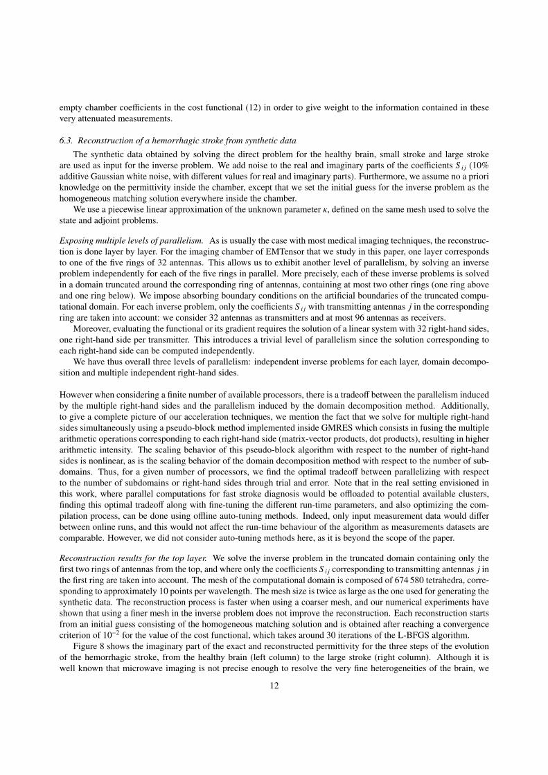
Figure 8 shows the imaginary part of the exact and reconstructed permittivity for the three steps of the evolutionof the hemorrhagic stroke, from the healthy brain (left column) to the large stroke (right column). Although it iswell known that microwave imaging is not precise enough to resolve the very fine heterogeneities of the brain, we

12

Figure 8: Top row: imaginary part of the exact permittivity for the healthy brain, small and large hemorrhagic strokes (indicated by the blackarrow). Bottom row: corresponding reconstructions obtained by solving the inverse problem for the top layer.

can see that the reconstructed images enable to track the evolution of the hemorrhagic stroke. More precisely, wecan identify the appearance of the small stroke, even though the variations on the transmission coefficients betweenhealthy brain and small stroke are very small as seen in Figure 7 (top). It is difficult to assess quantitatively the qualityof the reconstruction for low resolution imaging techniques such as microwave imaging; pointwise comparisons arenot really meaningful. For this reason, we report in Table 2 the mean value of the reconstructed permittivity (exactpermittivity in parentheses) in the ellipsoidal stroke region and its variation between healthy brain, small stroke andlarge stroke. We can see that although we do not quantitatively recover the exact values of the permittivity, the trendand order of magnitude of the variations are preserved in the reconstructions.

permittivity healthy brain small stroke large strokereal part imag. part real part imag. part real part imag. part

mean value 43.2 (44.4) 15.4 (16.3) 45.7 (56.2) 18.6 (30.2) 51.6 (56.3) 23.6 (29.6)

variation healthy→ small small→ large+6% (+27%) +20% (+85%) +13% (+22%) +41% (+75%)

Table 2: Mean value of the reconstructed permittivity in the ellipsoidal stroke region and variation of the permittivity between healthy brain andsmall stroke (in the small ellipsoid) and between small and large stroke (in the large ellipsoid). Values for the exact permittivity are reported inparentheses.

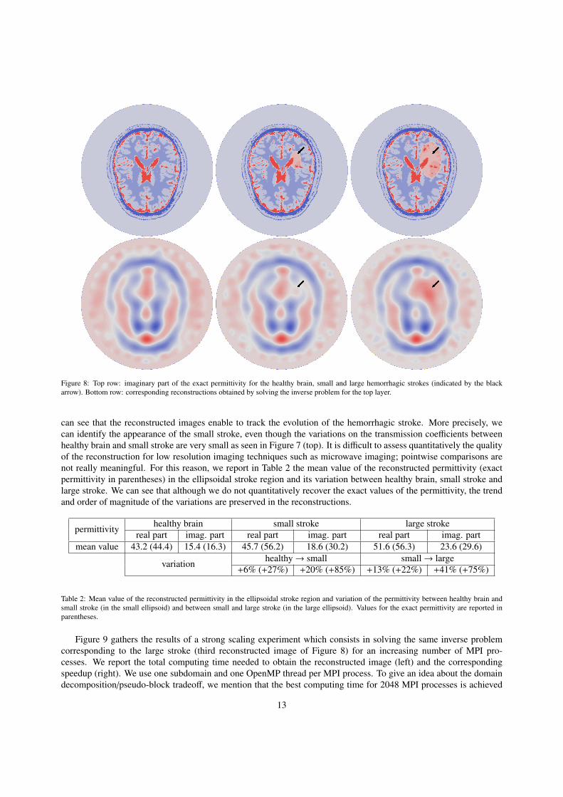
Figure 9 gathers the results of a strong scaling experiment which consists in solving the same inverse problemcorresponding to the large stroke (third reconstructed image of Figure 8) for an increasing number of MPI pro-cesses. We report the total computing time needed to obtain the reconstructed image (left) and the correspondingspeedup (right). We use one subdomain and one OpenMP thread per MPI process. To give an idea about the domaindecomposition/pseudo-block tradeoff, we mention that the best computing time for 2048 MPI processes is achieved

13

64 128 256 512 1 0242 048

4 096

0.5

1

2

4

8

16

# of MPI processes

Tim

ein

min

utes

Linear speedup

64 128 256 512 1 0242 048

4 096

1

2

4

8

16

32

64

# of MPI processes

Spee

dup

Linear speedup

Figure 9: Strong scaling experiment: total time needed to obtain the third reconstructed image shown in Figure 8 (left) and corresponding speedup(right).

by using 8 domain decomposition communicators (i.e. 8 concurrent direct solves) with 256 subdomains treating 4right-hand sides each. In contrast to the strong scaling experiment for the direct problem in Section 6.1, we obtainsublinear speedups for the inverse problem. This can be explained by the fact that the solution phase dominates theoverall cost, with the setup phase being less prevalent. Indeed, linear systems to be solved in the inverse problem aresmaller, with multiple right-hand sides each. We thus observe deteriorating efficiency, as the one-level domain de-composition preconditioner is not perfectly numerically scalable (increase in terms of number of GMRES iterations)at large process counts, where the setup cost is the smallest.

Nevertheless, Figure 9 shows that we can generate an image with a total computing time of less than 2 minutes(94 seconds) using 4096 cores. These preliminary results are very encouraging as they show that we are able toachieve a satisfactory reconstruction time in the perspective of using such an imaging technique for monitoring. Thisallows clinicians to obtain almost instantaneous images 24/7 or on demand. Although the reconstructed images donot feature the complex heterogeneities of the brain, which is in accordance with what we expect from microwaveimaging methods, they allow the characterization of the stroke and its monitoring, at least on synthetic data.

7. Conclusion

We have developed a tool that reconstructs a microwave tomographic image of the brain in less than 2 minutesusing 4096 cores. This computational time corresponds to clinician acceptance for rapid diagnosis or medical moni-toring at the hospital. These images were obtained from noisy synthetic data from a very accurate model of the brain.To our knowledge, this is the first time that such a realistic study (operational acquisition device, highly accurate three-dimensional synthetic data, 10% noise) shows the feasibility of microwave imaging. This study was made possible bythe use of massively parallel computers and facilitated by the HPDDM and FreeFem++ tools that we have developed.The next step is the validation of these results on clinical data.

Regarding the numerical aspects of this work, we will accelerate the solution of the series of direct problems,which accounts for more than 80% of our elapsed time. We explain here the three main avenues of research:

• The present ORAS solver for Maxwell’s equations is a one level algorithm, which cannot scale well overthousands of subdomains. The introduction of a two-level preconditioner with an adequate coarse space wouldallow for very good speedups even for decompositions into a large number of subdomains.

• Recycling information obtained during the convergence of the optimization algorithm will also enable us toimprove the performance of the method, see [21].

14

• Iterative block methods that allow for simultaneous solutions of linear systems have not been fully investigated.Arithmetic intensity would be increased since block methods may converge in a smaller number of iterationswhile exploiting modern computer architectures effectively.

Acknowledgments

This work was granted access to the HPC resources of TGCC@CEA under the allocations 2016-067519 and2016-067730 made by GENCI. This work has been supported in part by ANR through project MEDIMAX, ANR-13-MONU-0012.

[1] J. C. Lin, M. J. Clarke, Microwave imaging of cerebral edema, Proceedings of the IEEE 70 (5) (1982) 523–524.[2] S. Y. Semenov, D. R. Corfield, Microwave tomography for brain imaging: feasibility assessment for stroke detection, International Journal of

Antennas and Propagation.[3] S. Semenov, B. Seiser, E. Stoegmann, E. Auff, Electromagnetic tomography for brain imaging: from virtual to human brain, in: 2014 IEEE

Conference on Antenna Measurements & Applications (CAMA), 2014.[4] S. Mustafa, B. Mohammed, A. Abbosh, Novel preprocessing techniques for accurate microwave imaging of human brain, IEEE Antennas

and Wireless Propagation Letters 12 (2013) 460–463.[5] X. Li, E. J. Bond, B. D. Van Veen, S. C. Hagness, An overview of ultra-wideband microwave imaging via space-time beamforming for

early-stage breast-cancer detection, IEEE Antennas and Propagation Magazine 47 (1) (2005) 19–34.[6] A. Zamani, A. M. Abbosh, A. T. Mobashsher, Fast frequency-based multistatic microwave imaging algorithm with application to brain injury

detection, IEEE Transactions on Microwave Theory and Techniques 64 (2) (2016) 653–662.[7] C. Pichot, P. Lobel, L. Blanc-Feraud, M. Barlaud, K. Belkebir, J.-M. Elissalt, J.-M. Geffrin, Gradient and Newton-Kantorovich methods for

microwave tomography, in: Inverse Problems in Medical Imaging and Nondestructive Testing, Springer, 1997, pp. 168–187.[8] N. Irishina, A. Torrente, Brain stroke detection by microwaves using prior information from clinical databases, in: Abstract and Applied

Analysis, Vol. 2013, Hindawi, 2013.[9] R. Beck, R. Hiptmair, Multilevel solution of the time-harmonic Maxwell’s equations based on edge elements, International Journal for

Numerical Methods in Engineering 45 (7) (1999) 901–920.[10] J.-C. Nedelec, Mixed finite elements in R3, Numerische Mathematik 35 (3) (1980) 315–341.[11] V. Dolean, P. Jolivet, F. Nataf, An Introduction to Domain Decomposition Methods: algorithms, theory and parallel implementation, SIAM,

2015.[12] F. Pellegrini, J. Roman, SCOTCH: A Software Package for Static Mapping by Dual Recursive Bipartitioning of Process and Architecture

Graphs, in: High-Performance Computing and Networking, Springer, 1996, pp. 493–498.[13] G. Karypis, V. Kumar, A fast and high quality multilevel scheme for partitioning irregular graphs, SIAM Journal on Scientific Computing

20 (1) (1998) 359–392.[14] A. St-Cyr, M. J. Gander, S. J. Thomas, Optimized multiplicative, additive, and restricted additive Schwarz preconditioning, SIAM Journal on

Scientific Computing 29 (6) (2007) 2402–2425).[15] B. Despres, P. Joly, J. E. Roberts, A domain decomposition method for the harmonic Maxwell equations, in: Iterative methods in linear

algebra (Brussels, 1991), North-Holland, Amsterdam, 1992, pp. 475–484.[16] F. Hecht, New development in FreeFem++, Journal of Numerical Mathematics 20 (3-4) (2012) 251–265.[17] P. Jolivet, V. Dolean, F. Hecht, F. Nataf, C. Prud’homme, N. Spillane, High-performance domain decomposition methods on massively

parallel architectures with FreeFem++, Journal of Numerical Mathematics 20 (3-4) (2012) 287–302.[18] P. Jolivet, F. Hecht, F. Nataf, C. Prud’homme, Scalable domain decomposition preconditioners for heterogeneous elliptic problems, in: Proc.

of the Int. Conference on High Performance Computing, Networking, Storage and Analysis, IEEE, 2013, pp. 1–11.[19] O. Schenk, K. Gartner, Solving unsymmetric sparse systems of linear equations with PARDISO, Future Generation Computer Systems 20 (3)

(2004) 475–487.[20] P. Amestoy, I. Duff, J.-Y. L’Excellent, J. Koster, A fully asynchronous multifrontal solver using distributed dynamic scheduling, SIAM Journal

on Matrix Analysis and Applications 23 (1) (2001) 15–41.[21] M. L. Parks, E. De Sturler, G. Mackey, D. D. Johnson, S. Maiti, Recycling Krylov Subspaces for Sequences of Linear Systems, SIAM Journal

on Scientific Computing 28 (5) (2006) 1651–1674.

15