53
Midterm Review Session
| Date post: | 18-Dec-2015 |
| Category: |
Documents |
| View: | 219 times |
| Download: | 1 times |

Midterm Review Session

Things to Review
• Concepts
• Basic formulae
• Statistical tests

Things to Review
• Concepts
• Basic formulae
• Statistical tests

Populations <-> Parameters;Samples <-> Estimates

Nomenclature
Population
Parameter
Sample
Statistics
Mean
Variance s2
Standard Deviation
s€
x

In a random sample, each member of a population has an
equal and independent chance of being
selected.

Review - types of variables
• Categorical variables
• Numerical variablesDiscrete
Continuous
Nominal
Ordinal

Reality
Result
Ho true Ho false
Reject Ho
Do not reject Ho correct
correctType I error
Type II error

Sampling distribution of the mean, n=10
Sampling distribution of the mean, n=100
Sampling distribution of the mean, n = 1000


Things to Review
• Concepts
• Basic formulae
• Statistical tests

Things to Review
• Concepts
• Basic formulae
• Statistical tests
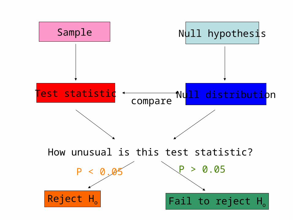
Sample
Test statistic
Null hypothesis
Null distributioncompare
How unusual is this test statistic?
P < 0.05 P > 0.05
Reject Ho Fail to reject Ho

Statistical tests
• Binomial test• Chi-squared goodness-of-fit
– Proportional, binomial, poisson
• Chi-squared contingency test• t-tests
– One-sample t-test– Paired t-test– Two-sample t-test

Statistical tests
• Binomial test• Chi-squared goodness-of-fit
– Proportional, binomial, poisson
• Chi-squared contingency test• t-tests
– One-sample t-test– Paired t-test– Two-sample t-test

Quick reference summary: Binomial test
• What is it for? Compares the proportion of successes in a sample to a hypothesized value, p
o
• What does it assume? Individual trials are randomly sampled and independent
• Test statistic: X, the number of successes
• Distribution under Ho: binomial with parameters n and
po.
• Formula:
P(x) = probability of a total of x successesp = probability of success in each trialn = total number of trials
€
P(x) =n
x
⎛
⎝ ⎜
⎞
⎠ ⎟px 1− p( )
n−x
P = 2 * Pr[xX]

Sample
Test statisticx = number of successes
Null hypothesisPr[success]=po
Null distributionBinomial n, po
compare
How unusual is this test statistic?
P < 0.05 P > 0.05
Reject Ho Fail to reject Ho
Binomial test

Binomial test

Statistical tests
• Binomial test• Chi-squared goodness-of-fit
– Proportional, binomial, poisson
• Chi-squared contingency test• t-tests
– One-sample t-test– Paired t-test– Two-sample t-test

Quick reference summary: 2 Goodness-of-Fit test
• What is it for? Compares observed frequencies in categories of a single variable to the expected frequencies under a random model
• What does it assume? Random samples; no expected values < 1; no more than 20% of expected values < 5
• Test statistic: 2
• Distribution under Ho: 2 with
df=# categories - # parameters - 1• Formula:
€
2 =Observedi − Expectedi( )
2
Expectediall classes
∑

Sample Null hypothesis:Data fit a particular
Discrete distribution
Null distribution:2 With
N-1-param. d.f.
compare
How unusual is this test statistic?
P < 0.05 P > 0.05
Reject Ho Fail to reject Ho
2 goodness of fit test
Calculate expected values
Test statistic
€
2 =Observedi − Expectedi( )
2
Expectediall classes
∑
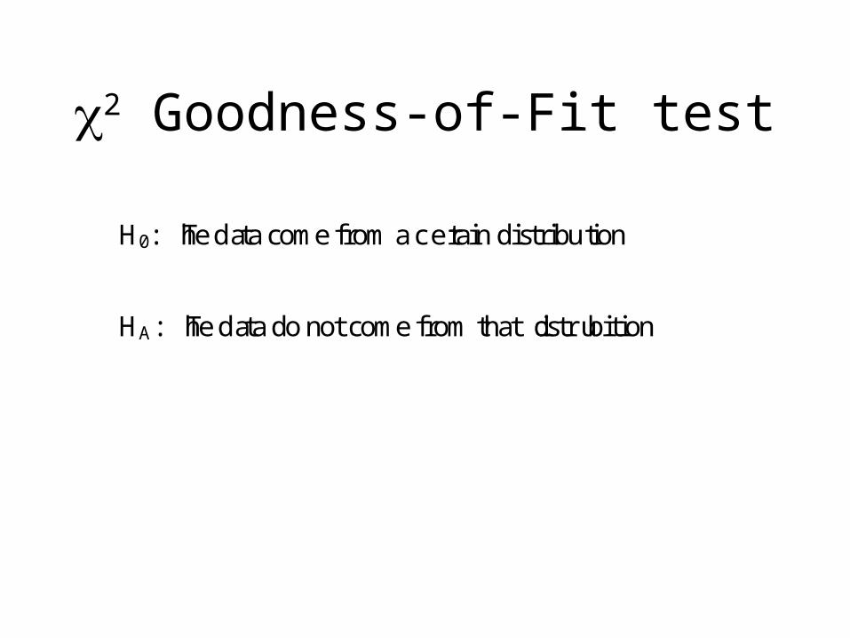
2 Goodness-of-Fit test
H0: The data come from a certain distribution
HA: The data do not come from that distrubition

Possible distributions
€
Pr X[ ] =e−μ μ X
X!€
Pr[x] =n
x
⎛
⎝ ⎜
⎞
⎠ ⎟px 1− p( )
n−x
Pr[x] = n * frequency of occurrence

Proportional
Binomial
Poisson
Given a number of categories Probability proportional to number of opportunitiesDays of the week, months of the year
Number of successes in n trialsHave to know n, p under the null hypothesisPunnett square, many p=0.5 examples
Number of events in interval of space or timen not fixed, not given pCar wrecks, flowers in a field

Statistical tests
• Binomial test• Chi-squared goodness-of-fit
– Proportional, binomial, poisson
• Chi-squared contingency test• t-tests
– One-sample t-test– Paired t-test– Two-sample t-test

Quick reference summary: 2 Contingency Test
• What is it for? Tests the null hypothesis of no association between two categorical variables
• What does it assume? Random samples; no expected values < 1; no more than 20% of expected values < 5
• Test statistic: 2
• Distribution under Ho: 2 with
df=(r-1)(c-1) where r = # rows, c = # columns
• Formulae:
€
2 =Observedi − Expectedi( )
2
Expectediall classes
∑
€
Expected =RowTotal *ColTotal
GrandTotal

Sample Null hypothesis:No association
between variables
Null distribution:2 With
(r-1)(c-1) d.f.
compare
How unusual is this test statistic?
P < 0.05 P > 0.05
Reject Ho Fail to reject Ho
2 Contingency Test
Calculate expected values
Test statistic
€
2 =Observedi − Expectedi( )
2
Expectediall classes
∑

2 Contingency test
H0: There is no association between these two variables
HA: There is an association between these two variables

Statistical tests
• Binomial test• Chi-squared goodness-of-fit
– Proportional, binomial, poisson
• Chi-squared contingency test• t-tests
– One-sample t-test– Paired t-test– Two-sample t-test

Quick reference summary: One sample t-test
• What is it for? Compares the mean of a numerical variable to a hypothesized value, μ
o
• What does it assume? Individuals are randomly sampled from a population that is normally distributed.
• Test statistic: t
• Distribution under Ho: t-distribution with n-1 degrees of
freedom.• Formula:
€
t =Y − μo
SEY

SampleNull hypothesis
The population mean is equal to
o
One-sample t-test
Test statistic Null distributiont with n-1 dfcompare
How unusual is this test statistic?
P < 0.05 P > 0.05
Reject Ho Fail to reject Ho
€
t =Y − μo
s / n

One-sample t-test
Ho: The population mean is equal to o
Ha: The population mean is not equal to o
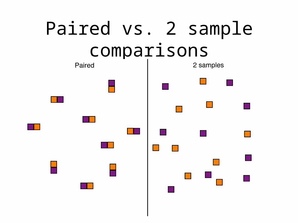
Paired vs. 2 sample comparisons

Quick reference summary: Paired t-test
• What is it for? To test whether the mean difference in a population equals a null hypothesized value, μ
do
• What does it assume? Pairs are randomly sampled from a population. The differences are normally distributed
• Test statistic: t
• Distribution under Ho: t-distribution with n-1 degrees of
freedom, where n is the number of pairs• Formula:
€
t =d − μdo
SEd

SampleNull hypothesis
The mean differenceis equal to
o
Paired t-test
Test statistic Null distributiont with n-1 df
*n is the number of pairscompare
How unusual is this test statistic?
P < 0.05 P > 0.05
Reject Ho Fail to reject Ho
€
t =d − μdo
SEd

Paired t-test
Ho: The mean difference is equal to 0
Ha: The mean difference is not equal 0

Quick reference summary: Two-sample t-test
• What is it for? Tests whether two groups have the same mean
• What does it assume? Both samples are random samples. The numerical variable is normally distributed within both populations. The variance of the distribution is the same in the two populations
• Test statistic: t
• Distribution under Ho: t-distribution with n1+n2-2
degrees of freedom.• Formulae:
€
t =Y 1 −Y 2SE
Y 1−Y 2
€
SEY 1 −Y 2
= sp2 1
n1
+1
n2
⎛
⎝ ⎜
⎞
⎠ ⎟
€
sp2 =
df1s12 + df2s2
2
df1 + df2

SampleNull hypothesis
The two populations have the same mean
1
2
Two-sample t-test
Test statistic Null distributiont with n1+n2-2 dfcompare
How unusual is this test statistic?
P < 0.05 P > 0.05
Reject Ho Fail to reject Ho
€
t =Y 1 −Y 2SE
Y 1−Y 2

Two-sample t-test
Ho: The means of the two populations are equal
Ha: The means of the two populations are not equal

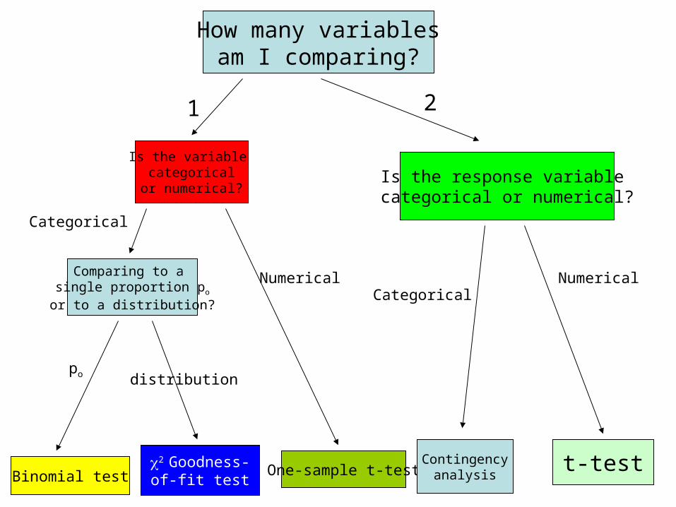
Which test do I use?

How many variablesam I comparing?
1
2
Methods for a single variable
Methods forcomparing two
variables
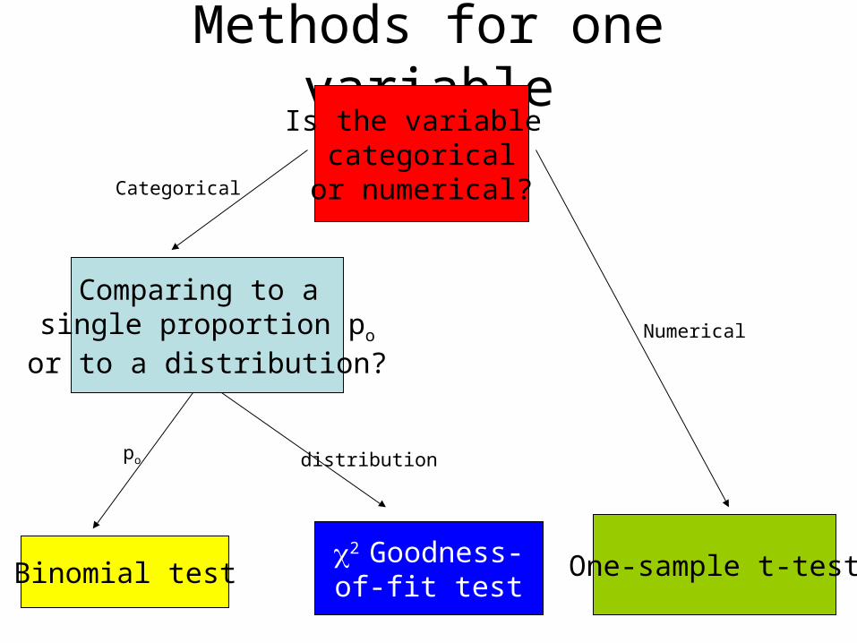
Methods for one variableIs the variable
categoricalor numerical?
Comparing to a single proportion po
or to a distribution?
Binomial test2 Goodness-
of-fit testOne-sample t-test
Categorical
Numerical
po distribution

Methods for two variables
Explanatory variableResponse variable Categorical Numerical
CategoricalContingency tableGrouped bar graph
Mosaic plot
NumericalMultiple histograms
Cumulative frequency distributionsScatter plot
X
Y

Methods for two variables
Explanatory variableResponse variable Categorical Numerical
CategoricalContingency tableGrouped bar graph
Mosaic plot
NumericalMultiple histograms
Cumulative frequency distributionsScatter plot
X
Y
Contingencyanalysis
t-test
Logistic regression
Regression

Methods for two variables
Is the response variable categorical or numerical?
Contingencyanalysis
t-test
Categorical Numerical
1 2
How many variablesam I comparing?
Is the variable categorical
or numerical?
Comparing to a single proportion po
or to a distribution?
Binomial test2 Goodness-
of-fit testOne-sample t-test
Categorical
Numerical
po distribution
Is the response variable categorical or numerical?
t-test
Categorical
Contingencyanalysis
Numerical
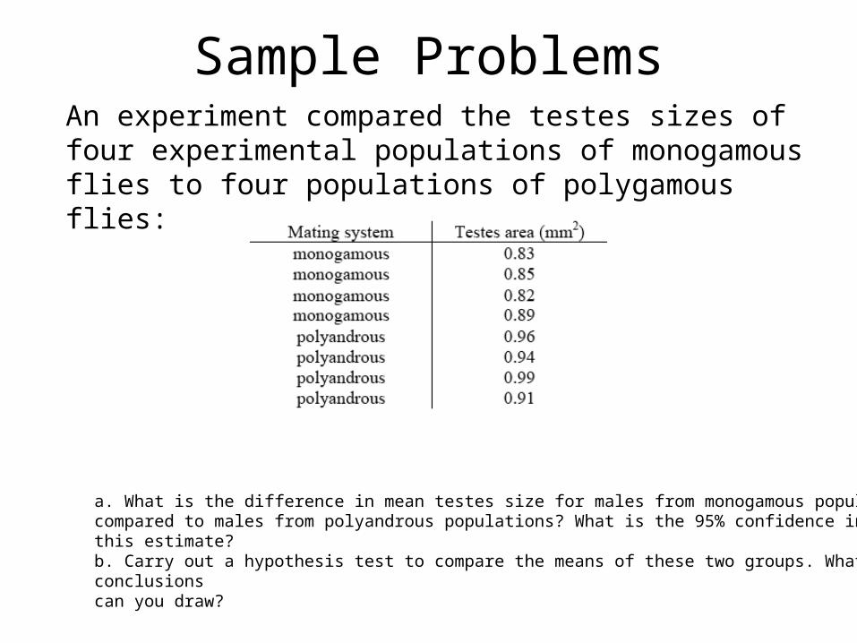
Sample ProblemsAn experiment compared the testes sizes of four experimental populations of monogamous flies to four populations of polygamous flies:
a. What is the difference in mean testes size for males from monogamous populationscompared to males from polyandrous populations? What is the 95% confidence interval forthis estimate?b. Carry out a hypothesis test to compare the means of these two groups. What conclusionscan you draw?

Sample Problems
In Vancouver, the probability of rain during a winter day is 0.58, for a spring day 0.38, for a summer day 0.25, and for a fall day 0.53. Each of these seasons lasts one quarter of the year.
What is the probability of rain on a randomly-chosen day in Vancouver?

Sample problemsA study by Doll et al. (1994) examined the relationship between moderate intake of alcohol and the risk of heart disease. 410 men (209 "abstainers" and 201 "moderate drinkers") were observed over a period of 10 years, and the number experiencing cardiac arrest over this period was recorded and compared with drinking habits. All men were 40 years of age at the start of the experiment. By the end of the experiment, 12 abstainers had experienced cardiac arrest whereas 9 moderate drinkers had experienced cardiac arrest.
Test whether or not relative frequency of cardiac arrest was different in the two groups of men.

Sample Problems
An RSPCA survey of 200 randomly-chosen Australian pet owners found that 10 said that theyhad met their partner through owning the pet.
A. Find the 95% confidence interval for the proportionof Australian pet owners who find love through their pets.
B. What test would you use to test if the true proportion is significantly different from 0.01? Write the formula that you would use to calculate a P-value.

Sample Problems
One thousand coins were each flipped 8 times, and the number of heads was recorded for each coin. Here are the results:
Does the distribution of coin flips match the distribution expected with fair coins? ("Fair coin" means that the probability of heads per flip is 0.5.)Carry out a hypothesis test.

Sample problemsVertebrates are thought to be unidirectional in growth, with size either increasing or holdingsteady throughout life. Marine iguanas from the Galápagos are unusual in a number of ways, and ateam of researchers has suggested that these iguanas might actually shrink during the low foodperiods caused by El Niño events (Wikelski and Thom 2000). During these events, up to 90% of theiguana population can die from starvation. Here is a plot of the changes in body length of 64surviving iguanas during the 1992-1993 El Niño event.
The average change in length was −5.81mm, with standard deviation 19.50mm.
Test the hypothesis that length did not change on average during the El Niño event.


